Evaluating Posterior Distributions by Selectively Breeding Prior Samples

Abstract

Using Markov chain Monte Carlo to sample from posterior distributions was the key innovation which made Bayesian data analysis practical. Notoriously, however, MCMC is hard to tune, hard to diagnose, and hard to parallelize. This pedagogical note explores variants on a universal non-Markov-chain Monte Carlo scheme for sampling from posterior distributions. The basic idea is to draw parameter values from the prior distributions, evaluate the likelihood of each draw, and then copy that draw a number of times proportional to its likelihood. The distribution after copying is an approximation to the posterior which becomes exact as the number of initial samples goes to infinity; the convergence of the approximation is easily analyzed, and is uniform over Glivenko-Cantelli classes. While not entirely practical, the schemes are straightforward to implement (a few lines of R), easily parallelized, and require no rejection, burn-in, convergence diagnostics, or tuning of any control settings. I provide references to the prior art which deals with some of the practical obstacles, at some cost in computational and analytical simplicity.

Suppose we have a prior probability measure $\Pi_{0}$ on $\Theta$, and a likelihood function $f(\theta,x)$. (Since $x$ plays little further role in what follows, I suppress it in the notation.) We want to sample from the posterior measure $\Pi_{1}$, defined via Bayes’s rule:

$$\Pi_{1}(A)=\frac{\Pi_{0}(fA)}{\Pi_{0}(f)}$$

using the de Finetti notation for expectations, so that $\Pi_{0}(fA)=\int{f(\theta)\mathbf{1}_{A}(\theta)d\Pi_{0}(\theta)}$. I explain how to obtain a sample from $\Pi_{1}$, supposing only that we can draw an IID sample from $\Pi_{0}$, and that we can calculate the likelihood. I first develop a weighted sampling scheme, and then consider ways of producing unweighted samples.

The inspiration for the algorithms below lies in the following observation. If $\Pi_{0}$ and $\Pi_{1}$ have densities $\pi_{0}$ and $\pi_{1}$, then Bayes’s rule takes the form

$$\pi_{1}(\theta)=\frac{f(\theta)\pi_{0}(\theta)}{\Pi_{0}(f)}$$

and this is exactly the form of the “replicator equation” of evolutionary biology, which describes the effects of natural selection on the gene pool of a population (Shalizi, 2009, Appendix A). In the evolutionary interpretation, $\theta$ refers to genotypes rather than parameter values, and $f(\theta)$ is not likelihood but “fitness”, the mean number of surviving offspring left by individuals of genotype $\theta$ (Hofbauer and Sigmund, 1998). Usually, in biology, the fitness of any one genotype is “frequency-dependent”, i.e., a function of the whole distribution of genotypes, but this is excluded in Bayes’s rule.

Bayesian updating describes an evolutionary process in an infinitely large population without competition, cooperation, mutation or sex. The algorithms below are all variants on taking this literally with a finite population.

Very similar algorithms have of course been published before; §4.2 provides references, and §§4.3–4.4 discusses some of their pros and cons.

1 Fitness-Weighted Samples

The fitness-weighted algorithm is very simple.

Algorithm 1: Likelihood Importance Prior Sampling (LIPS)

1. Draw $n$ samples $\theta_{1},\theta_{2},\ldots\theta_{n}$ iidly from $\Pi_{0}$.

2. For each $\theta_{i}$, calculate the likelihood $f(\theta_{i})$.

3. Approximate $\Pi_{1}$ by

   $$\widehat{\Pi}_{1}=\frac{\sum_{i=1}^{n}{f(\theta_{i})\delta_{\theta_{i}}}}{\sum_{j=1}^{n}{f(\theta_{j})}}$$ (1)

In particular, the posterior probability of any measurable set $A\subset\Theta$ is approximated by

$$\widehat{\Pi}_{1}(A)=\frac{\sum_{i=1}^{n}{f(\theta_{i})\mathbf{1}_{A}(\theta_{i})}}{\sum_{j=1}^{n}{f(\theta_{j})}}$$ (2)

Clearly, $\widehat{\Pi}_{1}$ is a probability measure. It converges on $\Pi_{1}$ as $n$ grows:

Proposition 1

Suppose $\Pi_{1}(f)>0$. Then as $n\rightarrow\infty$, $\widehat{\Pi}_{1}(A)\rightarrow\Pi_{1}(A)$ almost surely $(\Pi_{0})$.

Proof: Divide both the numerator and denominator of Eq. 2 by $n$:

$$\widehat{\Pi}_{1}(A)=\frac{n^{-1}\sum_{i=1}^{n}{f(\theta_{i})\mathbf{1}_{A}(\theta_{i})}}{n^{-1}\sum_{j=1}^{n}{f(\theta_{j})}}$$

Call the numerator $N_{A}$ and the denominator $D$. Since $\theta_{i}$ are IID, by the law of large numbers, $N_{A}\rightarrow\Pi_{0}(fA)$ and $D\rightarrow\Pi_{0}(f)$ almost surely. By the continuous mapping theorem for almost-sure convergence, then, $N_{A}/D\rightarrow\Pi_{0}(fA)/\Pi_{0}(f)=\Pi_{1}(A)$. $\Box$

By the usual measure-theoretic arguments, Proposition 1 extends from measurable sets to integrable functions.

Corollary 1

Suppose $\Pi_{1}(f)>0$, and that $\Theta$ is a locally compact, second-countable Hausdorff (lcscH) space, such as $\mathbb{R}^{d}$. Then as $n\rightarrow\infty$, $\widehat{\Pi}_{1}\stackrel{{\scriptstyle D}}{{\rightarrow}}\Pi_{1}$ almost surely $(\Pi_{0})$.

Proof: Take any finite collection of sets $A_{1},A_{2},\ldots A_{k}$ which are all continuity sets for $\Pi_{1}$, i.e., sets whose boundaries $\partial A_{i}$ have $\Pi_{1}$ measure 0. By Proposition 1, $\widehat{\Pi}_{1}(A_{i})\rightarrow\Pi_{1}(A_{i})$ a.s. ($\Pi_{0}$). For any finite $k$, therefore, $(\widehat{\Pi}_{1}(A_{1}),\ldots\widehat{\Pi}_{1}(A_{k}))\rightarrow(\Pi_{1}(A_{1}),\ldots\Pi_{1}(A_{k}))$ a.s. ($\Pi_{0}$). Since the convergence holds almost surely, a fortiori it holds in distribution. But now by Kallenberg (2002, Theorem 16.16(iii)), $\widehat{\Pi}_{1}\stackrel{{\scriptstyle D}}{{\rightarrow}}\Pi_{1}$. $\Box$

There is also a Glivenko-Cantelli-type result.

Corollary 2

Suppose that $\Theta$ is Borel-isomorphic to a complete, separable metric (“Polish”) space, and that $\mathcal{F}$ is a bounded, separable family of measurable functions on $\Theta$, where either the bracketing or covering number of $\mathcal{F}$ is finite under every measure on $\Theta$. Then, with $\Pi_{0}$-probability 1,

$$\sup_{f\in\mathcal{F}}{\left|\widehat{\Pi}_{1}(f)-\Pi_{1}(f)\right|}\rightarrow 0$$

Proof: Finite bracketing number and finite covering number are equivalent to each other and to the universal Glivenko-Cantelli property, by van Handel (2013, Theorem 1.3). The combination of these assumptions with Proposition 1 thus meets sufficient condition (6) of van Handel (2013, Corollary 1.4), and the result follows. $\Box$

1.1 Large-Sample Asymptotics

We may say more about the rate of convergence of $\widehat{\Pi}_{1}(A)$ to $\Pi_{1}(A)$.

Proposition 2

Suppose $\Pi_{0}(f)>0$. Then

$$n\mathrm{Var}\left[\widehat{\Pi}_{1}(A)\right]\rightarrow\frac{\Pi_{0}(f^{2})\Pi_{1}^{2}(A)+\Pi_{0}(f^{2}A)(1-2\Pi_{1}(A))}{\Pi_{0}^{2}(f)}$$

where the variance is taken over the drawing of the $\theta_{i}$ from $\Pi_{0}$.

Proof: Defining $N_{A}$ and $D$ as in the proof of Proposition 1, the delta method gives an asymptotic variance:

$$\mathrm{Var}\left[\widehat{\Pi}_{1}(A)\right]\rightarrow{\left(\frac{\partial\widehat{\Pi}_{1}(A)}{\partial N_{A}}\right)}^{2}\mathrm{Var}\left[N_{A}\right]+{\left(\frac{\partial\widehat{\Pi}_{1}(A)}{\partial D}\right)}^{2}\mathrm{Var}\left[D\right]+2\frac{\partial\widehat{\Pi}_{1}(A)}{\partial N_{A}}\frac{\partial\widehat{\Pi}_{1}(A)}{\partial D}\mathrm{Cov}\left[N_{A},D\right]$$ (3)

Fill in each piece, using the fact that an indicator function is equal to its own square:

$$\frac{\partial\widehat{\Pi}_{1}(A)}{\partial N_{A}} = \frac{1}{D}\rightarrow\frac{1}{\Pi_{0}(f)}$$ (4)

$$\frac{\partial\widehat{\Pi}_{1}(A)}{\partial D} = -\frac{N_{A}}{D^{2}}\rightarrow-\frac{\Pi_{0}(fA)}{\Pi_{0}^{2}(f)}$$ (5)

$$\mathrm{Var}\left[N_{A}\right] = n^{-1}(\Pi_{0}(f^{2}A^{2})-\Pi_{0}^{2}(fA))=n^{-1}(\Pi_{0}(f^{2}A)-\Pi_{0}^{2}(fA))$$ (6)

$$\mathrm{Var}\left[D\right] = n^{-1}(\Pi_{0}(f^{2})-\Pi_{0}^{2}(f))$$ (7)

$$\mathrm{Cov}\left[N_{A},D\right] = n^{-1}(\Pi_{0}(f^{2}A)-\Pi_{0}(fA)\Pi_{0}(f))$$ (8)

Put these together, and pull out the common factor of $n$:

$$n\mathrm{Var}\left[\widehat{\Pi}_{1}(A)\right] \rightarrow \frac{\Pi_{0}(f^{2}A)-\Pi_{0}^{2}(fA)}{\Pi_{0}^{2}(f)}$$

$$+\frac{\Pi_{0}^{2}(fA)(\Pi_{0}(f^{2})-\Pi_{0}^{2}(f))}{\Pi_{0}^{4}(f)}$$

$$-2\frac{\Pi_{0}(fA)}{\Pi_{0}^{3}(f)}(\Pi_{0}(f^{2}A)-\Pi_{0}(fA)\Pi_{0}(f))$$

Since $\Pi_{1}(A)=\Pi_{0}(fA)/\Pi_{0}(f)$, after some algebra,

$$n\mathrm{Var}\left[\widehat{\Pi}_{1}(A)\right]\rightarrow\Pi_{1}^{2}(A)\frac{\Pi_{0}(f^{2})}{\Pi_{0}^{2}(f)}+\frac{\Pi_{0}(f^{2}A)(1-2\Pi_{1}(A))}{\Pi_{0}^{2}(f)}$$

as was claimed. $\Box$

Remarks, or sanity checks: (i) $1\geq 1-2\Pi_{1}(A)\geq-1$, and $\Pi_{0}(f^{2})\geq\Pi_{0}(f^{2}A)$, so the numerator is always $\geq 0$. (ii) As $A\rightarrow\emptyset$ or $A\rightarrow\Theta$, the variance $\rightarrow 0$. (iii) As $\Pi_{1}(A)\rightarrow 1$, the variance tends to $\Pi_{0}(f^{2}A^{c})/\Pi_{0}^{2}(f)$, while as $\Pi_{1}(A)\rightarrow 0$, the numerator approaches $\Pi_{0}(f^{2}A)/\Pi_{0}^{2}(f)$. (iv) An oracle which could sample directly from $\Pi_{1}$ would have an asymptotic variance proportional to $\Pi_{1}(A)-\Pi_{1}^{2}(A)$, so the algorithm is not as efficient as the oracle.

Corollary 3

Suppose $\Pi_{0}(f)>0$. Then for any set $A$,

$$\lim_{n}{n\mathrm{Var}\left[\widehat{\Pi}_{1}(A)\right]}\leq 2\frac{\Pi_{0}(f^{2})}{\Pi_{0}^{2}(f)}=2\exp{D_{2}(\Pi_{1}\|\Pi_{0})}$$

where $D_{2}$ is the Rényi (1961) divergence of order 2.

Proof: Since $\Pi_{0}(f^{2}A)(1-2\Pi_{1}(A))\leq\Pi_{0}(f^{2})$, the previous proposition gives us an asymptotic variance of at most $2\Pi_{0}(f^{2})/\Pi_{0}^{2}(f)$ for any set. Now, the Rényi divergence of order $\alpha\geq 0$ is defined (for $\alpha\neq 0,1,\infty$) to be (van Erven and Harremoës, 2014)

$$D_{\alpha}(P\|Q)=\frac{1}{\alpha-1}\log{P\left({\left(\frac{dP}{dQ}\right)}^{\alpha-1}\right)}$$

Pick $\alpha=2$, and suppose without loss of generality that $P$ and $Q$ have densities $p$ and $q$ with respect to a common measure $M$, such as $(P+Q)/2$, so $\frac{dP}{dQ}(\theta)=p(\theta)/q(\theta)$. Then

$$D_{2}(P\|Q)=\log{P\left(\frac{p}{q}\right)}=\log{M\left(\frac{p^{2}}{q}\right)}=\log{Q\left(\frac{p^{2}}{q^{2}}\right)}$$

Set $P=\Pi_{1}$ and $Q=\Pi_{0}$. The density ratio is

$$\frac{p(\theta)}{q(\theta)}=\frac{f(\theta)}{\Pi_{0}(f)}$$

so

$$D_{2}(\Pi_{1}\|\Pi_{0})=\log{\Pi_{0}\left(\frac{f^{2}(\theta)}{\Pi_{0}^{2}(f)}\right)}=\log{\frac{\Pi_{0}(f^{2})}{\Pi_{0}^{2}(f)}}$$

Undoing the logarithm proves the result. $\Box$

1.2 High-Information Asymptotics

The preceding results deal with the behavior as the number of Monte Carlo samples $n$ grows; to sum up (Corollary 3), with a large number of draws from the prior, the accuracy of the approximation is controlled by $\Pi_{0}(f^{2})/\Pi_{0}^{2}(f)=1+\mathrm{Var}\left[f\right]/\Pi_{0}^{2}(f)$. There is also a second asymptotic regime of interest, which is when the observation $x$ becomes highly informative. It would be somewhat perverse if the approximation broke down just when the observation became most useful.

These fears can be calmed, at least in some situations, by asymptotic expansions. Suppose that $\Theta=\mathbb{R}^{d}$ and $\Pi_{0}$ has a density $\pi_{0}$ with respect to Lebesgue measure, so $\Pi_{0}(g)=\int{g(\theta)\pi_{0}(\theta)d\theta}$. In particular, write

$$\Pi_{0}(f)=\int{\pi_{0}(\theta)\exp{\left\{-t\ell(\theta)\right\}}d\theta}$$

and

$$\Pi_{0}(f^{2})=\int{\pi_{0}(\theta)\exp{\left\{-2t\ell(\theta)\right\}}d\theta}$$

where $t$ gauges, in some relevant sense, how informative the observation $x$ is, with the normalized negative log-likelihood $\ell(\theta)$ converging to a constant-magnitude function as $t\rightarrow\infty$. ($t$ may represent the number of measurements taken, the length of a time series, the precision of a measuring instrument, etc.). Assume that $\ell(\theta)$ has a unique interior minimum at the MLE $\hat{\theta}$. We may then appeal to Laplace approximation to evaluate these integrals: by Eq. 2.3 in Tierney et al. (1989):

$$\Pi_{0}(f)=(2\pi)^{d/2}|\Sigma|^{1/2}f(\hat{\theta})\left(\pi_{0}(\hat{\theta})+A_{1}t^{-1}\right)+O(t^{-2})$$

where $\Sigma$ is the inverse Hessian matrix of $\ell$ at $\hat{\theta}$. The precise expression for $A_{1}$ in terms of the derivatives of $\pi_{1}$ and $\ell$ is known (Wojdylo, 2006; Nemes, 2013) but not, for the present purposes, illuminating. Appealing to Laplace approximation a second time,

$$\Pi_{0}(f^{2})=(2\pi)^{d/2}|\Sigma/2|^{1/2}f^{2}(\hat{\theta})\left(\pi_{0}(\hat{\theta})+A_{2}t^{-1}\right)+O(t^{-2})$$

Thus

$$\frac{\Pi_{0}(f^{2})}{\Pi_{0}^{2}(f)} = \frac{(2\pi)^{d/2}|\Sigma/2|^{1/2}f^{2}(\hat{\theta})\left(\pi_{0}(\hat{\theta})+A_{2}t^{-1}\right)+O(t^{-2})}{\left[(2\pi)^{d/2}|\Sigma|^{1/2}f(\hat{\theta})\left(\pi_{0}(\hat{\theta})+A_{1}t^{-1}\right)+O(t^{-2})\right]^{2}}$$ (10)

$$= (4\pi)^{-(d/2)}\frac{\pi_{0}(\hat{\theta})+A_{1}t^{-1}+O(t^{-2})}{\pi_{0}^{2}(\hat{\theta})+2A_{2}\pi_{0}(\hat{\theta})t^{-1}+O(t^{-2})}$$ (11)

$$= \frac{(4\pi)^{-(d/2)}}{\pi_{0}(\hat{\theta})}\frac{1+\frac{A_{1}}{\pi_{0}(\hat{\theta})}t^{-1}+O(t^{-2})}{1+2\frac{A_{2}}{\pi_{0}(\hat{\theta})}t^{-1}+O(t^{-2})}$$ (12)

$$= \frac{(4\pi)^{-(d/2)}}{\pi_{0}(\hat{\theta})}\left(1+\frac{A_{1}-2A_{2}}{\pi_{1}(\hat{\theta})t}\right)+O(t^{-2})$$ (13)

The upshot of this is calculation is that as $t\rightarrow\infty$, that is, as the data becomes increasingly informative, the ratio $\Pi_{0}(f^{2})/\Pi_{0}^{2}(f)$ tends to a limit proportional to the prior density at the MLE, with vanishing corrections. Heuristically, as $t\rightarrow\infty$, both $\Pi_{0}(f^{2})$ and $\Pi_{0}(f)$ become integrals dominated by their slowest-decaying integrand. The rate of exponential decay is twice as fast for $f^{2}$ as for $f$, so $\Pi_{0}(f^{2})/\Pi_{0}^{2}(f)$ tends to a $t$-independent limit. The real source of a difficulty, if there is one, is $\pi_{0}(\hat{\theta})$ being small.

It’s worth remarking that (in the present notation) $\log{\pi_{1}(\hat{\theta})/\pi_{0}(\hat{\theta})}$ was proposed by Haldane (1954, pp. 483, 486) as a measure of the intensity of natural selection on a population.

1.3 Sketch of Finite-Sample Bounds

It would be nice if there were finite-sample concentration results to go along with these asymptotics. One approach to this would be to use results developed for weighting training samples to cope with distributional shift. The most nearly applicable result is that of Cortes et al. (2010, Theorem 7 and Corollary 1), which runs (in the present notation) as follows. If the samples $\theta_{1},\ldots\theta_{n}$ are drawn iidly from $Q$, and $dP/dQ=w$, then over any function class $H$ bounded between 0 and 1,

$$\mathbb{P}\left(\sup_{h\in H}{\frac{P(h)-n^{-1}\sum_{i=1}^{n}{w(\theta_{i})h(\theta_{i})}}{\sqrt{Q(w^{2})}}}>\epsilon\right)\leq 4G_{H}(2n)e^{-n\epsilon^{8/3}/4^{5/3}}$$

where $G_{H}$ is the growth function of $H$, the number of ways a set of $n$ points can be dichotomized by sets from $H$ (Anthony and Bartlett, 1999). As in this result, we sample from one distribution and want to compute integrals under another probability measure, so we would like to set $Q=\Pi_{0}$ and $P=\Pi_{1}$. (This would make the denominator on the left hand side $\exp{\left\{D_{2}(\Pi_{1}\|\Pi_{0})/2\right\}}$.) Standing in the way is the annoyance that the conversion weights $w=f(\theta)/\Pi_{0}(f)$ are unavailable, because instead of $\Pi_{0}(f)$ we only have a Monte Carlo approximation $D$. Introduce a new random measure $R$, defined through $dR/d\Pi_{0}=f/D$. ($R$ is not, generally, a properly normalized probability measure.) The theorem of Cortes et al. then bounds the deviation of $\widehat{\Pi}_{1}(h)$ from $R(h)$. Since $d\Pi_{1}/dR=D/\Pi_{0}(f)$, a finite-sample deviation inequality for $D$ will yield a bound on the relative deviation of $\widehat{\Pi}_{1}(h)$ from $\Pi_{1}(h)$. Controlling the convergence of $D$ to $\Pi_{0}(f)$ will need assumptions on the distribution (under the prior) of likelihoods, which seem too model-specific to pursue here.

2 Unweighted Samples

Weighted samples are fine for many purposes, and simple to analyze, but there are times when it is nicer to not have to keep track of weights. There are several ways of modifying the algorithm to give us unweighted samples.

Algorithm 2, Likelihood-Amplified Prior Sampling (LAPS)

1. Draw $n$ samples $\theta_{1},\theta_{2},\ldots\theta_{n}$ iidly from $\Pi_{0}$.

2. For each $\theta_{i}$, calculate the likelihood $f(\theta_{i})$.

3. Fix a constant $c>0$, and make $\left\lceil cf(\theta_{i})\right\rceil$ copies of $\theta_{i}$.

4. Put all the copies of all the $\theta_{i}$ together in a multi-set or bag $\tilde{\theta}$.

5. Use the empirical distribution of $\tilde{\theta}$, $\tilde{\Pi}_{1}$ as the approximation to $\Pi_{1}$.

$\tilde{\Pi}_{1}$ can be viewed as forcing the weights on take on discrete values which are separated by a scale that depends on $c$. (Specifically, the weights must be multiples of $1/\sum_{i}{\lceil cf(\theta_{i})\rceil}$.) One thus has that $\tilde{\Pi}_{1}(A)=\widehat{\Pi}_{1}(A)+O(1/c)$. Making $c$ very large will however also tend to make $\tilde{\theta}$ large and computationally awkward. One fix for that would be to draw a sub-sample from $\tilde{\theta}$, but if we were going to do that, the intermediate phase of making lots of copies is unnecessary.

Algorithm 3, Selective Likelihood-Amplified Prior Sampling (SLIPS)

1. Draw $n$ samples $\theta_{1},\theta_{2},\ldots\theta_{n}$ iidly from $\Pi_{0}$.

2. For each $\theta_{i}$, calculate the likelihood $f(\theta_{i})$.

3. Sample $m$ times from the $\theta_{i}$, with replacement, and with sampling weights proportional to $f(\theta_{i})$. Call this sample $\theta^{\dagger}$.

4. Return the empirical distribution of $\theta^{\dagger}$, $\Pi^{\dagger}_{1}$, as the approximation to $\Pi_{1}$.

$\Pi^{\dagger}_{1}$ will approach $\widehat{\Pi}_{1}$ as $m\rightarrow\infty$ (Douc and Moulines, 2007, Theorem 3), but $m$ can be tuned to trade off numerical accuracy against memory demands.

3 Implementation

All three algorithms can be implemented in one short piece of R.

rposterior <- function(n, rprior, likelihood, c = 100, m = n, mode = "lips") {
    theta <- rprior(n)
    likelihoods <- apply(theta, 1, likelihood)
    if (mode == "lips") {
        integrated.likelihood <- sum(likelihoods)
        posterior.weights <- likelihoods/integrated.likelihood
    } else if (mode == "laps") {
        copies <- ceiling(c * likelihoods)
        theta <- theta[rep(1:n, times = copies), ]
        posterior.weights = rep(1, times = sum(copies))
    } else if (mode == "slips") {
        theta <- theta[sample(1:n, size = m, replace = TRUE, prob = likelihoods),
            ]
        posterior.weights = rep(1, times = m)
    }
    return(list(theta = theta, posterior.weights = posterior.weights))
}

Here the argument rprior is a function which, given an input n, returns a 2D array of n IID parameter vectors drawn from the prior distribution, each sample on its own row. Similarly, the likelihood function must, given a parameter vector, return the likelihood. This code could be improved in many ways — e.g., it makes no attempt to take advantage of parallelized back-ends if they are available — but shows off the simplicity of the idea, and will suffice for an example.

Example: Gaussian Likelihood and Gaussian Prior

Let us take a case where the posterior can be computed in closed form, for purposes of comparison. The observations will have a Gaussian distribution with unknown mean $\theta$ and variance 1, and the prior measure on the measure is itself $\Pi_{0}=N(0,1)$. The posterior distribution is then $\Pi_{1}=N(x/2,1/2)$. Figure 1 shows how well the scheme works in this simple setting.

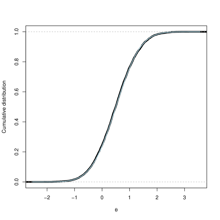
rprior <- function(n) {
    matrix(rnorm(n, mean = 0, sd = 1), nrow = n)
}
likelihood <- function(theta) {
    dnorm(x = 1, mean = theta, sd = 1)
}
theta <- rposterior(10000, rprior = rprior, likelihood = likelihood, mode = "slips")
plot(ecdf(theta$theta), main = "", xlab = expression(theta), ylab = "Cumulative distribution",
    lwd = 5)
curve(pnorm(x, 0.5, 1/sqrt(2)), col = "lightblue", add = TRUE, lwd = 2)

Figure 1: Example of breeding MC samples for a simple normal-normal example. Black line: CDF of the MC samples after breeding. Blue line: analytic posterior. Here we set $x=1$ for the observation.

In the preceding paragraph, the prior distribution was not that different from the posterior. We thus consider the case where we have taken ${10}^{4}$ IID samples, so that $\overline{X}|\theta\sim N(\theta,{10}^{-4})$. The analytic posterior is then $\theta|\overline{X}\sim N(\frac{{10}^{4}}{{10}^{4}+1}\overline{X},1/10001)$. The quality of the approximation is still quite good (Figure 2), and, of course, will only get better as $n$ increases.

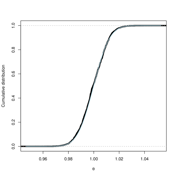
likelihood2 <- function(theta) {
    dnorm(x = 1, mean = theta, sd = 1/sqrt(10000))
}
theta2 <- rposterior(1e+05, rprior, likelihood2, mode = "slips")
plot(ecdf(theta2$theta), main = "", xlab = expression(theta), ylab = "Cumulative distribution",
    lwd = 5)
curve(pnorm(x, (10000/(10000 + 1) * 1), sqrt(1/(10000 + 1))), col = "lightblue",
    add = TRUE, lwd = 2)

Figure 2: Continuation of the Gaussian-Gaussian example, where we suppose that we have taken ${10}^{4}$ uncorrelated observations, each with $\sigma^{2}=1$, and $\overline{x}=1$.

4 Discussion

4.1 Summary

For any measurable $A\subseteq\Theta$, $\widehat{\Pi}_{1}(A)=\Pi_{1}(A)+O_{P}(1/\sqrt{n})$. Thus Algorithm 1 provides a rapidly-converging way of estimating posterior probabilities. The error of approximation is controlled by $D_{2}(\Pi_{1}\|\Pi_{0})$, or more concretely by the ratio $\Pi_{0}(f^{2})/\Pi_{0}^{2}(f)=1+\mathrm{Var}\left[f\right]/\Pi_{0}^{2}(f)$. This is to say, the more (prior) variance there is in the likelihood, the worse this will work. (The dimensionality of $\Theta$ is not, however, directly relevant.) Algorithms 2 and 3 simply introduce additional approximation error, which however can be made as small as desired either by letting $c\rightarrow\infty$ or $m\rightarrow\infty$.

4.2 Related Work

These algorithms are all closely related to particle filters (Doucet et al., 2001), which however usually aim at approximating a sequence of probability measures which themselves evolve randomly, and where convergence results often rely on the ergodicity of the underlying process. Here, however, we have only one (possibly high-dimensional) observation, and only one posterior distribution to match.

Artificial intelligence employs many population-based optimization techniques to explore fitness landscapes, by copying more successful solutions in proportion to their fitness, most notably genetic algorithms (Holland, 1975; Mitchell, 1996). All of these, however, have a vital role for operations which introduce new members of the population, corresponding to mutation, cross-over, sex, etc., which are necessarily lacking in Bayesian updating, and avoided in the algorithms set forth above.

Beyond these general points of inspiration, Rubin (1987) proposed what is basically Algorithm 3 as a way of doing multiple imputation, as opposed to sampling from the posterior of the parameters. Cappé et al. (2004) is an even more precise anticipation, though their use of sequential importance sampling means they aren’t just sampling from the prior, with attendant loss of simplicity and analytical tractability.

4.3 Advantages

Best practices in Markov chain Monte Carlo counsel discarding all the samples from an initial burn-in period, running diagnostic tests to check converge to the equilibrium, etc. (Admittedly, some doubt the value of these steps: see Geyer 1992.) None of this is needed or even applicable here: all that’s needed is for $n$ to be large enough that $\widehat{\Pi}_{1}$ and/or $\tilde{\Pi}_{1}$ is a good approximation to the posterior distribution $\Pi_{1}$. Moreover, there is no need to pick or adjust proposal distributions. Indeed, there aren’t really any control settings that need to be tuned, since it’s straightforward that $n$, $c$ and $m$ should all be as large as possible.

Implementing this scheme requires only the ability to draw IID samples from the prior $\Pi_{0}$, and to compute the likelihood function $f$. The former tends to be straightforward, at least when the prior is expressed hierarchically. Actually, examination of the proofs will confirm that we do not even need to calculate $f$; it would be enough to calculate something proportional to the likelihood, $r(x)f(\theta)$, where the factor of proportionality $r(x)>0$ and is strictly constant in $\theta$. That being said, calculating the likelihood can be difficult for complex models, but this is outside the scope here.

One special advantage of this scheme is that it lends itself readily to parallelization, which MCMC does not. Drawing iidly from the prior is “embarrassingly” parallel. Calculating $f(\theta_{i})$ is also embarrassingly parallel, requiring no communication between the different $\theta_{i}$, as is making copies of them. Every step in algorithm 2 is embarrassingly parallel, though with large $c$ we might need a lot of memory in each node. Algorithms 1 and 3 require us to compute $\sum_{i=1}^{n}{f(\theta_{i})}$, which does require communication, but finding the sum of $n$ numbers is among the first parallelized algorithms taught to beginners (Burch, 2009, §2.1), so this might not be much of a drawback.

4.4 Disadvantages

The great advantage of all three algorithms is that the only distribution they ever need to draw from is the prior, and priors are typically constructed to make that easy. The corresponding disadvantage is that they can spend a lot of time evaluating the likelihood of parameter values which have in fact very low likelihood, and so end up making a small contribution to the posterior. MCMC, by contrast, preferentially spends most of its time in regions of high posterior density.

Three observations may, however, lessen this contrast. First, while the output of MCMC follows the posterior distribution, its proposals do not, and the likelihood must be evaluated once for each proposal. Thus it is not clear that, in general, MCMC has a computational advantage on this score. Second, while I have not explored it in this brief note, it should be possible to short-cut the evaluation of the likelihood of very hopeless parameter points, as in the “go with the winners” of Grassberger (2002), or the “austerity” of Korattikara et al. (2014). Third, the problematic case is where most of the posterior probability mass is concentrated in a region of very low prior mass. Numerical evidence from trying out more complicated situations than the Gaussian prior-and-likelihood suggests that this can be a serious issue, which is why I do not advocate these algorithms, in their present form, as a replacement for MCMC (note that the non-Markov chain “population Monte Carlo” of Cappé et al. (2004) does not suffer from this drawback). It is, however, at least arguable that what goes wrong in these situation isn’t that these algorithms converge slowly, but that the priors are bad, and should be replaced by less misleading ones (Gelman and Shalizi, 2013).

Acknowledgments

Thanks to my students in 36-350, introduction to statistical computing, for driving me to this way of explaining Bayes’s rule, and to John Miller for many valuable conversations about the connections between adaptive population processes and Monte Carlo. I was supported while writing this by grants from the NSF (DMS1207759, DMS1418124) and from the Institute for New Economic Thinking. §§1.1 and 1.2 were worked out during breaks in the proceedings while serving as a juror in January 2014, and so also supported by jury duty pay.

References

- Anthony and Bartlett (1999) Anthony, Martin and Peter L. Bartlett (1999). Neural Network Learning: Theoretical Foundations. Cambridge, England: Cambridge University Press.
- Bengtsson et al. (2008) Bengtsson, Thomas, Peter Bickel and Bo Li (2008). “Curse-of-dimensionality revisited: Collapse of the particle filter in very large scale systems.” In Probability and Statistics; Essays in Honor of David A. Freedman (Deborah Nolan and Terry Speed, eds.), pp. 316–334. Brentwood, Ohio: Institute of Mathematical Statistics. URL http://projecteuclid.org/euclid.imsc/1207580091. doi:10.1214/imsc/1207580069.
- Burch (2009) Burch, Carl (2009). “Introduction to Parallel and Distributed Algorithms.” Electronic manuscript. URL http://www.cburch.com/books/distalg/.
- Cappé et al. (2004) Cappé, Olivier, Arnaud Guillin, Jean-Michel Marin and Christian P. Robert (2004). “Population Monte Carlo.” Journal of Computational and Graphical Statistics, 13: 907–929. URL https://basepub.dauphine.psl.eu/handle/123456789/6072. doi:10.1198/106186004X12803.
- Cortes et al. (2010) Cortes, Corinna, Yishay Mansour and Mehryar Mohri (2010). “Learning Bounds for Importance Weights.” In Advances in Neural Information Processing 23 [NIPS 2010] (John Lafferty and C. K. I. Williams and John Shawe-Taylor and Richard S. Zemel and A. Culotta, eds.), pp. 442–450. Cambridge, Massachusetts: MIT Press. URL http://papers.nips.cc/paper/4156-learning-bounds-for-importance-weighting.
- Douc and Moulines (2007) Douc, Randal and Eric Moulines (2007). “Limit Theorems for Weighted Samples with Applications to Sequential Monte Carlo Methods.” ESIAM: Proceedings, 19: 101–107. URL http://arxiv.org/abs/math.ST/0507042. doi:10.1051/proc:071913.
- Doucet et al. (2001) Doucet, Arnaud, Nando de Freitas and Neil Gordon (eds.) (2001). Sequential Monte Carlo Methods in Practice. Berlin: Springer-Verlag.
- Gelman and Shalizi (2013) Gelman, Andrew and Cosma Rohilla Shalizi (2013). “Philosophy and the Practice of Bayesian Statistics.” British Journal of Mathematical and Statistical Psychology, 66: 8–38. URL http://arxiv.org/abs/1006.3868. doi:10.1111/j.2044-8317.2011.02037.x.
- Geyer (1992) Geyer, Charles J. (1992). “Practical Markov Chain Monte Carlo.” Statistical Science, 7: 473–483. doi:10.1214/ss/1177011137.
- Grassberger (2002) Grassberger, Peter (2002). “Go with the Winners: a General Monte Carlo Strategy.” Computer Physics Communications, 147: 64–70. URL http://arxiv.org/abs/cond-mat/0201313. doi:10.1016/S0010-4655(02)00205-9.
- Haldane (1954) Haldane, J. B. S. (1954). “The Measurement of Natural Selection.” In Proceedings of the 9th International Congress of Genetics (G. Montalenti and A. Chiarugi, eds.), vol. 1, pp. 480–487. Florence: The Congress.
- Hofbauer and Sigmund (1998) Hofbauer, Josef and Karl Sigmund (1998). Evolutionary Games and Population Dynamics. Cambridge, England: Cambridge University Press.
- Holland (1975) Holland, John H. (1975). Adaptation in Natural and Artificial Systems: An Introductory Analysis with Applications to Biology, Control, and Artificial Intelligence. Ann Arbor, Michigan: University of Michigan Press, 1st edn.
- Kahn (1956) Kahn, Herman (1956). “Use of Different Monte Carlo Sampling Techniques.” In Symposion on the Monte Carlo Method (H. A. Meyer, ed.). New York: Wiley. URL http://www.rand.org/content/dam/rand/pubs/papers/2008/P766.pdf.
- Kallenberg (2002) Kallenberg, Olav (2002). Foundations of Modern Probability. New York: Springer-Verlag, 2nd edn.
- Korattikara et al. (2014) Korattikara, Anoop, Yutian Chen and Max Welling (2014). “Austerity in MCMC Land: Cutting the Metropolis-Hastings Budget.” In Proceedings of the 31st International Conference on Machine Learning 2014 [ICML 2014] (Eric P. Xing and Tony Jebara, eds.), pp. 181–189. URL https://proceedings.mlr.press/v32/korattikara14.html.
- Mitchell (1996) Mitchell, Melanie (1996). An Introduction to Genetic Algorithms. Cambridge, Massachusetts: MIT Press.
- Nemes (2013) Nemes, Gergő (2013). “An Explicit Formula for the Coefficients in Laplace’s Method.” Constructive Approximation, 38: 471–487. URL http://arxiv.org/abs/1207.5222. doi:10.1007/s00365-013-9202-6.
- Rényi (1961) Rényi, Alfréd (1961). “On Measures of Entropy and Information.” In Proceedings of the Fourth Berkeley Symposium on Mathematical Statistics and Probability (Jerzy Neyman, ed.), vol. 1, pp. 547–561. Berkeley: University of California Press. URL https://projecteuclid.org/proceedings/berkeley-symposium-on-mathematical-statistics-and-probability/Proceedings-of-the-Fourth-Berkeley-Symposium-on-Mathematical-Statistics-and/Chapter/On-Measures-of-Entropy-and-Information/bsmsp/1200512181.
- Rubin (1987) Rubin, Donald B. (1987). “A Noniterative Sampling/Importance Resampling Alternative to the Data Augmentation Algorithm for Creating a Few Imputations When Fractions of Missing Information Are Modest: The SIR Algorithm.” Journal of the American Statistical Association, 82: 543–546. URL http://www.jstor.org/stable/2289460.
- Shalizi (2009) Shalizi, Cosma Rohilla (2009). “Dynamics of Bayesian Updating with Dependent Data and Misspecified Models.” Electronic Journal of Statistics, 3: 1039–1074. URL http://arxiv.org/abs/0901.1342. doi:10.1214/09-EJS485.
- Tierney et al. (1989) Tierney, Luke, Robert E. Kass and Joseph B. Kadane (1989). “Fully Exponential Laplace Approximations to Expectations and Variances of Nonpositive Functions.” Journal of the American Statistical Association, 84: 710–716. URL http://www.stat.cmu.edu/~kass/papers/nonlinearFunctions.pdf.
- van de Geer (2000) van de Geer, Sara A. (2000). Empirical Processes in M-Estimation. Cambridge, England: Cambridge University Press.
- van Erven and Harremoës (2014) van Erven, Tim and Peter Harremoës (2014). “Rényi Divergence and Kullback-Leibler Divergence.” IEEE Transactions on Information Theory, 60: 3797–3820. URL http://arxiv.org/abs/1206.2459. doi:10.1109/TIT.2014.2320500.
- van Handel (2013) van Handel, Ramon (2013). “The Universal Glivenko-Cantelli Property.” Probability Theory and Related Fields, 155: 911–934. URL http://arxiv.org/abs/1009.4434. doi:10.1007/s00440-012-0416-5.
- Wojdylo (2006) Wojdylo, John (2006). “On the Coefficients that Arise from Laplace’s Method.” Journal of Computational and Applied Mathematics, 196: 241–266. doi:10.1016/j.cam.2005.09.004.