Event-triggered boundary control of $2\times 2$ semilinear hyperbolic systems

Abstract

We present an event-triggered boundary control scheme for hyperbolic systems. The trigger condition is based on predictions of the state on determinate sets, where the control input is only updated if the predictions deviate from the reference by a given margin. Closed-loop stability and absence of Zeno behaviour is established analytically. For the special case of linear systems, the trigger condition can be expressed in closed-form as an $L_{2}$-scalar product of kernels with the distributed state. The presented controller can also be combined with existing observers to solve the event-triggered output-feedback control problem. A numerical simulation demonstrates the effectiveness of the proposed approach.

I Introduction

We consider $2\times 2$ semilinear hyperbolic systems with one boundary actuator of the form

$$u_{t}(x,t) =-\lambda^{u}(x)\,u_{x}(x,t)+f^{u}(w(x,t),x),$$ (1)

$$v_{t}(x,t) =\phantom{-}\lambda^{v}(x)\,v_{x}(x,t)+f^{v}(w(x,t),x),$$ (2)

$$u(0,t) =g(v(0,t),t),$$ (3)

$$v(1,t) =U(t),$$ (4)

$$w(\cdot,0) =w_{0},$$ (5)

where $x\in[0,1]$, $t\geq 0$, $w(x,t)=\left(u(x,t),v(x,t)\right)$, subscripts denote partial derivatives, $U(t)$ is the control input, and $w_{0}$ the initial condition.

Systems of form (1)-(5) model a range of 1-d transport processes including gas or fluid flow through pipelines, open channel flow, traffic flow, electrical transmission lines, and blood flow in arteries [1]. Consequently, the control and observer design for such systems has received much attention.

Static controllers that achieve assymptotic convergence are designed using dissipative boundary conditions in [2] and using control Lyapunov functions in [3]. The exact-finite time controllability of such systems is analysed in [4, 5]. For the special case of linear systems, backstepping has become a popular method for designing feedback controllers that achieve this kind of performance. See, e.g., [6, 7, 8, 9, 10, 11, 12, 13] for a range of results using different configurations and stabilization or tracking as the objective. For semilinear and quasilinear systems, the same control performance has been achieved using a predictive approach [14, 15, 16, 17, 18].

Recently, there has been interest in the event-triggered boundary control of (linear) hyperbolic systems [19, 20, 21, 22]. The related topic of sampled-data control is analysed in [23]. In event-triggered control, the control inputs are held piecewise constant and are updated only when needed, instead of continuously in time or in a periodic fashion. One of the main benefits of such an approach is that it reduces wear and tear on the physical actuators, which is of interest in many applications. See also [24] for event-triggered control of ordinary differential equations (ODE).

The contribution of this paper is an event-triggered implementation of the predictive approach from [14]. For clarity of presentation, the focus is on the stabilisation of semilinear hyperbolic systems using state-feedback control, although the approach can readily be adapted to tracking problems, output-feedback control and quasilinear systems. Similarly, the extensions to $n+1$ systems (that is, vector-valued $u$ as considered in [25] for linear systems), and to time-varying $f^{u}$ and $f^{v}$ are straightforward.

The paper is structured as follows. Section II contains several preparations including the precise model assumptions, sufficient conditions for stability and well-posedness and the continuous-time implementation of the controller. The event-triggered controller is presented in Section III, including a closed-form implementation (i.e., without the need to solve PDEs online) for the special case of linear systems in Section III-A. Simulation examples are shown in Section IV and concluding remarks are given in Section V.

II Preliminaries

II-A Assumptions

We consider broad solutions to system (1)-(5), which are a type of weak solution defined by integrating (1)-(2) along characteristic lines and solving the obtained integral equations [26]. Well-posedness for broad solutions can be shown under the following assumptions.

The speeds $\lambda^{u},\lambda^{v}\in L^{\infty}([0,1])$ are assumed to be bounded from below and above by the finite values

$$\sup_{x\in[0,1]}\left(\min\{\lambda^{u}(x),\,\lambda^{v}(x)\}^{-1}\right) =k_{\Lambda^{-1}},$$ (6)

$$\sup_{x\in[0,1]}\max\{\lambda^{u}(x),\,\lambda^{v}(x)\} =k_{\Lambda}$$ (7)

The nonlinear functions $f^{u}$, $f^{v}$, and $g$ are globally Lipschitz-continuous in the state arguments, i.e.,

$$\operatorname*{ess\,sup}_{x\in[0,1],w\in\mathbb{R}^{2}}\max\left\{\|\partial_{w}f^{u}(w,x)\|_{\infty},\|\partial_{w}f^{v}(w,x)\|_{\infty}\right\}\ =l_{F},$$ (8)

$$\operatorname*{ess\,sup}_{v\in\mathbb{R},t\geq 0}|\partial_{v}g(v,t)|=l_{g},$$ (9)

where $\partial$ denotes partial derivatives and $l_{F}$ and $l_{g}$ are the finite Lipschitz constants. We assume further that the origin is an equilibrium, i.e.,

$$f^{u}(0,x) =f^{v}(0,x)=0 x\in[0,1],$$ for all (10)

$$g(0,t) =0 t\geq 0.$$ for all (11)

The initial conditions are assumed bounded with $w_{0}\in L^{\infty}([0,1],\mathbb{R}^{2})$.

Remark 1.

The global Lipschitz condition is restrictive, but made here to simplify some of the proofs. For locally Lipschiz-continuous data, similar local results can be shown. See also [5] for local controllability results.

II-B Characteristic lines and determinate sets

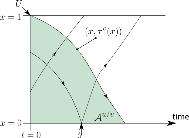
Figure 1: Characteristic lines for system (1)-(5) going upwards ($u$) and downwards ($v$). The area shaded in green indicates the determinate sets $\mathcal{A}^{u}(0)$ (including the line $(x,\tau^{v}(x))$) and $A^{v}(0)$ (excluding the line $(x,\tau^{v}(x))$) .

The effect of the control input $U(t)$ propagates through the domain $x\in[0,1]$ with finite speed $\lambda^{v}$. More precisely, the control input $U(t)$ entering at the boundary $x=1$ at time $t$ has an effect on the state at some location $x$ only after a delay of $\tau^{v}(x)$, where

$$\tau^{u}(x) =\int_{0}^{x}\frac{1}{\lambda^{u}(\xi)}d\xi, \tau^{v}(x) =\int_{x}^{1}\frac{1}{\lambda^{v}(\xi)}d\xi.$$ (12)

Consequently, the state on the determinate set can be predicted based on the current state at time $t$, $w(\cdot,t)$, where the determinate sets are given by

$$\mathcal{A}^{u}(t) =\{(x,s):\,x\in[0,1],\,s\in[t,t+\tau^{v}(x)]\},$$ (13)

$$\mathcal{A}^{v}(t) =\{(x,s):\,x\in[0,1],\,s\in[t,t+\tau^{v}(x))\}.$$ (14)

Lemma 2.

For any $t\geq 0$, the Cauchy problem consisting of (1)-(3) with $w(\cdot,t)$ as the initial condition at time $t$, has a unique solution $u(x,s)$ for $(x,s)\in\mathcal{A}^{u}(t)$ and $v(x,s)$ for $(x,s)\in\mathcal{A}^{v}(t)$. Moreover, there exists constant $c_{1}>0$ (depending on the model data) such that

$$\sup_{(x,s)\in\mathcal{A}^{u}(t)}|u(x,s)| \leq c_{1}\|w(\cdot,t)\|_{\infty},$$ (15)

$$\sup_{(x,s)\in\mathcal{A}^{v}(t)}|v(x,s)| \leq c_{1}\|w(\cdot,t)\|_{\infty}.$$ (16)

Proof.

The proof is given in [14, Appendix A]. See also [26, 27] for a general discussion of determinate sets. ∎

Remark 3.

One convenient implementation for determining the solution of $u(x,s)$ on $\mathcal{A}^{u}(t)$, including the solution on the line $u(x,t+\tau^{v}(x))$, $x\in[0,1]$, is to solve the system consisting of (1)-(4) with initial condition $w(\cdot,t)$ and an arbitrary input $U$ (e.g., $U\equiv\lim_{x\rightarrow 1}v(x,t)$) over the larger rectangular domain $[0,1]\times[t,t+\tau^{v}(0)]$. The solution of $u$ on $\mathcal{A}^{u}(t)$ can then be selected from the larger solution where, as seen in Lemma 2, it is independent of the choice for $U$.

II-C Sufficient condition for convergence

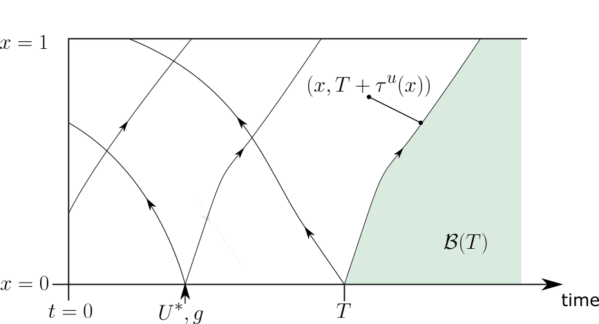
Figure 2: Characteristic lines for system (17)-(20).

Following [14], [17], we exploit that convergence to the origin is much easier to characterize via conditions on the uncontrolled boundary value $v(0,\cdot)$. In particular, we introduce the virtual input $U^{*}(t)$, which is the target value for $v(0,\cdot)$. We then reverse the roles of $t$ and $x$ in (1) and (2) to formulate the system as a PDE in the positive $x$-direction for $x\in[0,1]$.

$$u_{x}(x,t) =-\frac{1}{\lambda^{u}(x,t)}\,u_{t}(x,t)+\frac{f^{u}(w(x,t),x)}{\lambda^{u}(x)},$$ (17)

$$v_{x}(x,t) =\phantom{-}\frac{1}{\lambda^{v}(x,t)}\,v_{t}(x,t)-\frac{f^{v}(w(x,t),x)}{\lambda^{v}(x)},$$ (18)

$$v(0,t) =U^{*}(t),$$ (19)

$$u(0,t) =g(U^{*}(t),t).$$ (20)

See also Figure 2 for the characteristic lines of the transformed system (17)-(20). Using the same methodology underlying Lemma 2, it is possible to show the following:

Lemma 4.

For any $T\geq\tau^{v}(0)$, the transformed system (17)-(20) with $U^{*}(t)$ restricted to $t\geq T$, has unique solution on the set

$$\mathcal{B}(T)=\{(x,s):\,x\in[0,1],\,s\geq T+\tau^{u}(x)\},$$ (21)

independently of the initial condition $w_{0}$. Moreover, there exists constant $c_{2}>0$ (depending on the model data) such that

$$\sup_{(x,s)\in\mathcal{B}(T)}\|w(x,s)\|_{\infty}\leq c_{2}\,\sup_{s\geq T}|U^{*}(s)|.$$ (22)

Note that $[0,1]\times[T+\tau^{u}(1),\infty)\subset\mathcal{B}(T)$. Therefore, (22) implies that if $U^{*}(t)=0$ for all $t\geq T$, then $w(\cdot,t)=0$ for all $t\geq T+\tau^{u}(1)$.

II-D Continuous-time control design

The idea in [14] is to design $U(t)$ such that the future boundary value $v(0,t+\tau^{v}(0))$ becomes equal to the virtual input $U^{*}(t+\tau^{v}(0))$. By (22), if $v(0,t+\tau^{v}(0))=U^{*}(t+\tau^{v}(0))=0$ for all $t\geq T$, the state reaches the origin by time $T+\tau^{v}(0)+\tau^{u}(1)$.

Defining the future state on the characteristic line,

$$\bar{w}(x,t)=\left(\bar{u}(x,t),\bar{v}(x,t)\right)=w(x,t+\tau^{v}(x)),$$ (23)

the following relationship between $U$ and $v(0,t+\tau^{v}(0,t))$ is derived in [14, Theorem 2].

Lemma 5.

For given $\bar{u}$, the state $\bar{v}$ satisfies the ODE

$$\bar{v}_{x}(x,t) =-\frac{f^{v}((\bar{u}(x,t),\bar{v}(x,t)),x)}{\lambda^{v}(x)},$$ (24)

$$\bar{v}(1,t) =U(t).$$ (25)

Crucially, (24) is an ODE in the $x$-direction with no time-dynamics. Consequently, it can be solved in either $x$-direction. In (24)-(25), it is solved in the negative $x$ direction, so that $\bar{v}(0,t)$ is a function of $U(t)$. As originally explored in [14], the alternative is to start with the desired $U^{*}(t+\tau^{v}(0))$ and solve a copy of (24) in the positive $x$-direction, i.e., backwards relative to how the actual input $U$ propagates through the domain. By setting $U^{*}(t)\equiv 0$, the closed-loop system converges to the origin in finite (minimum) time.

Theorem 6.

Consider the system consisting of (1)-(5) in closed loop with $U(t)$ at each $t\geq 0$ set according to the following algorithm:

1. Predict $\bar{u}(\cdot,t)$ by solving (1)-(3) with $w(\cdot,t)$ as initial condition over the domain $\mathcal{A}^{u}(t)$;

2. Solve the target system

   $$\bar{v}^{*}_{x}(x,t) =-\frac{f^{v}((\bar{u}(x,t),\bar{v}^{*}(x,t)),x)}{\lambda^{v}(x)},$$ (26)

   $$\bar{v}^{*}(0,t) =0;$$ (27)

3. Set $U(t)=\bar{v}^{*}(1,t)$.

Then $w(\cdot,t)=0$ for all $t\geq\tau^{v}(0)+\tau^{u}(1)$.

Proof.

With $\bar{u}(\cdot,t)$ determined uniquely by the prediction in step 1), (24) and (26) are equivalent ODEs in $\bar{v}(\cdot,t)$ and $\bar{v}^{*}(\cdot,t)$, respectively. Since these ODEs have unique solution under the given assumptions, $\bar{v}(0,t)=\bar{v}^{*}(0,t)=0$ if and only if $U(t)=\bar{v}(1,t)=\bar{v}^{*}(1,t)$. That is, the construction in steps (1)-(3) ensures $v(0,t)=0$ for all $t\geq\tau^{v}(1)$. Convergence to the origin then follows from (22). ∎

III Event-triggered control

In this section, an event-triggered implementation of the controller from Section II-D is developed. That is, the control input is restricted to be piecewise constant with

$$U(t) =U(t_{k}) t\in[t_{k},t_{k+1})$$ for all (28)

where $t_{k}$, $k\in\mathbb{N}$, are the update times.

In the continuous-time implementation of the feedback controller, the control input is updated continuously so that the uncontrolled boundary value is kept at $v(0,t)=U^{*}(t)=0$ for $t\geq\tau^{v}(0)$. In the absence of any disturbances or prediction errors due to uncertainty, this ensures that the state is kept exactly at the origin. While such idealized assumptions are never exactly achievable in practice, it is usually also acceptable if the state remains sufficiently “close” to the origin. By the bound in (22), one can ensure that $\|w(\cdot,t)\|\leq\tilde{\epsilon}$ for any $\tilde{\epsilon}>0$ and sufficiently large $t$ by keeping $|v(0,t)|\leq\frac{\tilde{\epsilon}}{c_{2}}$. Therefore, the idea of the event-triggered control law is to compute the control inputs in the same way as in Theorem 6, but to only update the control input at times $t_{k}$ where the prediction of $|v(0,t_{k}+\tau^{v}(0))|$ under the previous control input exceeds some threshold $\varepsilon>0$.

We propose the following event-triggered feedback controller. At time $t>0$, given the state $w(\cdot,t)$ and threshold $\varepsilon$, the control input $U(t)$ is set according to the following algorithm, which is initialized with $\bar{U}=U(0)$ and $t_{0}=0$. The algorithm also produces the Zeno-free sequence of update times $t_{k}$, as established in Theorem 7.

1:  Predict $\bar{u}(\cdot,t)$ by solving (1)-(3) with state-measurement $w(\cdot,t)$ as initial condition over the domain $\mathcal{A}^{u}(t)$;

2:  Predict $v(0,t+\tau^{v}(0))=\bar{v}^{\circ}(0,t)$ under the current input by solving

$$\bar{v}_{x}^{\circ}(x,t) =-\frac{f^{v}((\bar{u}(x,t),\bar{v}^{\circ}(x,t)),x)}{\lambda^{v}(x)},$$ (29)

$$\bar{v}^{\circ}(1,t) =\bar{U};$$ (30)

3:  if $|\bar{v}^{\circ}(0,t)|>\varepsilon$ then

4:     solve target dynamics (26)-(27);

5:     set $\bar{U}=\bar{v}^{*}(1,t)$ and append update times by $t_{k+1}=t$;

6:  end if

7:  Set $U(t)=\bar{U}$.

Algorithm 1 Event-triggered control algorithm

Theorem 7.

The system consisting of (1)-(5) in closed-loop with $U(t)$ constructed by the event-triggered control algorithm above satisfies $|v(0,t)|\leq\varepsilon$ for all $t\geq\tau^{v}(0)$ and $\|w(\cdot,t)\|_{\infty}\leq c_{2}\,\varepsilon$ for all $t\geq\tau^{v}(0)+\tau^{u}(1)$. Moreover, there exists $\Delta>0$, which depends on $\varepsilon$, $\|w_{0}\|_{\infty}$ and the model data, such that $t_{k+1}-t_{k}\geq\Delta$ for all $k\in\mathbb{N}$.

Proof.

The construction is such that if $|\bar{v}(0,t)|>\varepsilon$, then $U$ is updated to a value such that $\bar{v}(0,t)$ becomes zero. The bound on $\|w(\cdot,t)\|_{\infty}$ for $t\geq\tau^{v}(0)+\tau^{u}(1)$ follows directly from (22). It only remains to be shown that $t_{k+1}-t_{k}\geq\Delta$. The idea of the proof is to show that for short $\Delta$ the solution to (29)-(30) at $x=0$ is continuous in time.

We first establish an a-priori bound on $\|w\|_{\infty}$. Choosing $\varepsilon<c_{1}\,\|w_{0}\|_{\infty}$ and using bound (16) we have that the closed-loop system satisfies $\|v(0,\cdot)\|_{\infty}\leq c_{1}\,\|w_{0}\|_{\infty}$. Thus, via bound (22) we obtain that $\|w\|_{\infty}\leq c_{1}\,c_{2}\,\|w_{0}\|_{\infty}$.

The control input $\bar{U}$ is first initialized at time $t=0$. Assuming $\bar{U}$ was last updated at time $t_{k}$, we show by induction that at least some fixed time $\Delta>0$ elapses before the update condition in line 3 of Algorithm 1 can be triggered.

We rewrite (29)-(30) as an integral equation with $\bar{u}$ playing the role of a parameter

$$\bar{v}^{\circ}[\bar{u}](x,t)=\bar{U}-\int_{1}^{x}\frac{f^{v}((\bar{u}(\xi,t),\bar{v}^{\circ}(\xi,t)),\xi)}{\lambda^{v}(\xi)}d\xi.$$ (31)

Due to the Lipschitz assumptions, the solution to (31) depends continuously on $\bar{u}$, i.e., there exists a constant $c_{3}$ such that

$$\|\bar{v}^{\circ}[\bar{u}_{1}]-\bar{v}^{\circ}[\bar{u}_{2}]\|_{\infty}\leq c_{3}\,\|\bar{u}_{1}-\bar{u}_{2}\|_{\infty}$$ (32)

Parameterize the characteristic lines of $u$ passing through a point $(x,t)$ via the solution of the ODE

$$\frac{d}{ds}z(x,t;s) =\lambda^{u}(z(x,t;s)), z(x,t;t) =x.$$ (33)

Then $u$ is continuous in $s$ along the characteristic line $(z(x,t;s),s)$ as long as $z(x,t;s)\in[0,1]$ (see [14, Section A.3]). In particular, $u$ satisfies

$$\frac{d}{dt}u(z(x,t_{k};t),t)=f^{u}(w(z(x,t_{k};t),t),z(x,t_{k};t)).$$ (34)

Hence,

$$|u(z(x,t_{k};t),t)-u(x,t_{k})|\leq c_{4}e^{c_{5}(t-t_{k})}$$ (35)

where $c_{4}$ scales linearly with $\|w\|_{\infty}$. Applying the same approach to the transformed system (23) gives

$$|\bar{u}(z(x,t_{k};t))-\bar{u}(x,t_{k})|\leq c_{4}e^{c_{5}(t-t_{k})}.$$ (36)

Define $\theta^{v}(x)=\int_{0}^{x}\frac{1}{\lambda^{v}(\xi)}d\xi$. Also define $y_{1}(t-t_{k})$ as the solution to the equation $\theta^{v}(y_{1})=t-t_{k}$, and $y_{2}(t-t_{k})$ as the solution to $\tau^{v}(y_{2})=t-t_{k}$. Then

$$|y_{1}(\Delta)| \leq\Delta\,k_{\Lambda} |1-y_{2}(\Delta)| \leq\Delta\,k_{\Lambda}.$$ and (37)

Figure 3: Schematic of the integrations paths and continuity of $u$ along its (upwards) characteristic lines in the proof of Theorem 7.

For all $\Delta<\tau^{u}(1)$, it follows that $z_{1}(\Delta)<1$ and $z_{2}(\Delta)>0$. So for any $x_{1}\in[z_{1}(t-t_{k}),1]$ there exists $x_{2}\in[0,z_{2}(t-t_{k})]$ such that $x_{1}=z(x_{2},t_{k};t)$. Using this, the integrals in (31) can be split into different parts (see also Figure 3) to obtain

$$|\bar{v}^{\circ}[\bar{u}(\cdot,t)](0,t)-\bar{v}^{\circ}[\bar{u}(\cdot,t_{k})](0,t_{k})|$$ (38)

$$=\left|\int_{0}^{y_{2}(t-t_{k})}\frac{f^{v}(\bar{w}(z(x,t_{k};t),t),z(x,t_{k};t))}{\lambda^{v}(z(x,t_{k};t))}\right.$$

$$\qquad-\frac{f^{v}(\bar{w}(x,t_{k}),x)}{\lambda^{v}(x)}dx$$

$$\quad+\int_{0}^{y_{1}(t-t_{k})}\frac{f^{v}(\bar{w}(x,t),x)}{\lambda^{v}(x)}dx$$

$$\left.\quad-\int_{y_{2}(t-t_{k})}^{1}\frac{f^{v}(\bar{w}(x,t_{k}),x)}{\lambda^{v}(x)}dx\right|=\left|I_{1}+I_{2}+I_{3}\right|,$$

where $U(t)-U(t_{k})=0$ has been used, and $I_{1}$, $I_{2}$ and $I_{3}$ are the first, second and third integrals, respectively. This can be bounded as follows. Due to the Lipschitz condition we have that

$$|I_{1}| \leq l_{F}k_{\Lambda^{-1}}\left(\|\bar{u}(\cdot,t)-\bar{u}(\cdot,t_{k})\|_{\infty}\right.$$ (39)

$$\hskip 51.21504pt+\left.\|\bar{v}^{\circ}[\bar{u}(\cdot,t)]-\bar{v}^{\circ}[\bar{u}(\cdot,t_{k})]\|_{\infty}\right)$$

$$\leq l_{F}k_{\Lambda^{-1}}(1+c_{3}\,)\|\bar{u}(\cdot,t)-\bar{u}(\cdot,t_{k})\|_{\infty},$$

where (32) is used in the last step. Due to (37) and using the Lipschitz conditions and the a-priori bound on $\|w\|$,

$$|I_{2}|\leq 2\,l_{F}k_{\Lambda^{-1}}c_{1}c_{2}k_{\Lambda}(t-t_{k}),$$ (40)

$$|I_{3}|\leq 2\,l_{F}k_{\Lambda^{-1}}c_{1}c_{2}k_{\Lambda}(t-t_{k}).$$ (41)

In summary, the integrals on the right-hand side of (38) are bounded and

$$|\bar{v}^{\circ}[\bar{u}(\cdot,t)](0,t)-\bar{v}^{\circ}[\bar{u}(\cdot,t_{k})](0,t_{k})|\leq h(t-t_{k})$$ (42)

with some continuous, strictly increasing function $h$ that satisfies $h(0)=0$ (where $h$ also depends on the a-priori bound on $\|w\|_{\infty}$, and thus, $\|w_{0}\|_{\infty}$ via the constant $c_{4}$). Therefore, there exists $\Delta>0$ such that $h(t-t_{k})\leq\varepsilon$ for all $t\leq t_{k}+\Delta$, which completes the proof. ∎

Remark 8 (State-dependent $\varepsilon$).

In Algorithm 1 the trigger-parameter $\varepsilon$ is chosen as a constant. An alternative implementation would be to choose $\varepsilon$ dependent on the state. The minimum inter-trigger time $\Delta$ decreases with increasing state norm. This could lead to frequent sampling if, e.g., the initial condition is far from the origin. In such situations it would likely be acceptable if the control specifications were relaxed, so that the state is first brought “closer” to the origin before the controller is tightened. For instance, if $\varepsilon=\frac{\gamma}{c_{2}}\|w(\cdot,t)\|_{\infty}$ with $\gamma<1$, then by (22) one has that $\|w(\cdot,t)\|_{\infty}$ reduces by at least $\gamma$ every $\tau^{v}(0)+\tau^{u}(1)$ units of time. That is, one would obtain exponential convergence. Such state dependent switching could also be combined with a minimum fixed $\varepsilon$ so that the system converges exponentially when it is outside a ball of certain size and is then only kept within that ball. The latter version would avoid switches that might be unnecessary if the system is already “close enough” to the origin, as implemented in Section IV.

Remark 9 (Periodic execution and robustness).

Instead of continuously measuring the state, performing the predictions in lines 1-2, and evaluating the trigger condition in line 3 of Algorithm 1, it would be more practicable to perform these steps only periodically at times $\tilde{t}_{i}=i\,\tilde{\Delta}$ with some sampling period $\tilde{\Delta}>0$. For instance, by choosing $\tilde{\Delta}<\Delta$ sufficiently small such that one can prove $|\bar{v}(0,\tilde{t}_{i+1})-\bar{v}(0,\tilde{t}_{i})|\leq\frac{1}{2}\varepsilon$, and replacing the trigger condition in line 3 by $|\bar{v}^{\circ}(0,\tilde{t}_{i})|>\frac{1}{2}\varepsilon$, it is possible to guarantee that if the update condition is not satisfied at time $\tilde{t}_{i}$, then the boundary value still satisfies $|\bar{v}(0,t)|\leq|\bar{v}(0,\tilde{t}_{i})|+\frac{1}{2}\varepsilon\leq\varepsilon$ for all $t\in[\tilde{t}_{i},\tilde{t}_{i+1}]$.

Similarly, one could account for prediction errors due to model uncertainty or disturbances by tightening the trigger condition further, so that the prediction $|\bar{v}^{\circ}(0,t)|$ plus an error term still remains below $\varepsilon$. The allowable uncertainties would then depend on $\varepsilon$ or, conversely, the achievable $\varepsilon$ would be limited by the given uncertainty. See the robustness result in [17].

Remark 10 (Reference tracking).

The developments above focus on stabilization of an equilibrium. Alternatively, tracking objectives of the form

$$v(0,t)=g_{\text{ref}}(t),$$ (43)

which includes many objectives of the form $\tilde{g}_{\text{ref}}(w(0,t),t)=0$ (substituting $u(0,t)$ by (3) and solving for $v(0,t)$), can be solved by replacing the boundary condition of the target system (26)-(27) by

$$\bar{v}^{*}_{x}(x,t) =-\frac{f^{v}((\bar{u}(x,t),\bar{v}^{*}(x,t)),x)}{\lambda^{v}(x)},$$ (44)

$$\bar{v}^{*}(0,t) =g_{\text{ref}}(t+\tau^{v}(0)),$$ (45)

and setting the trigger condition in line 3 of Algoruthm 1 to

$$|\bar{v}^{\circ}(0,t)-g_{\text{ref}}(t+\tau^{v}(0))|>\varepsilon.$$ (46)

III-A Closed-form expression for linear systems

Evaluating the trigger condition requires solving a nonlinear PDE online when predicting $\bar{u}(\cdot,t)$ and then solving an ODE to obtain $\bar{v}^{\circ}(0,t)$. As is the case for the continuous-time state-feedback controller [14, Section 3.4], it is possible to express the trigger condition as a simple integral of kernels (which can be precomputed) weighting the state.

Consider linear systems of the form

$$u_{t} =-\epsilon_{1}(x)u_{x}+c_{1}(x)v,$$ (47)

$$v_{t} =\epsilon_{2}(x)v_{x}+c_{2}(x)u,$$ (48)

$$v(1,t) =U(t),$$ (49)

$$u(0,t) =qv(0,t).$$ (50)

The derivations in [14, Section 3.4] can be modified slightly to show that the trigger condition can be evaluated via

$$\bar{v}^{\circ}(0,t)=\bar{U}-\int_{0}^{1} K^{vu}(1,\xi)u(\xi,t)-K^{vv}(1,\xi)v(\xi,t)d\xi,$$ (51)

where the kernels $K^{vu}$ and $K^{vv}$ are the solution of the PDE system given in [6, Equations (24)-(31)]. At each trigger instance, the control inputs can be updated as

$$\bar{U}=\int_{0}^{1}K^{vu}(1,\xi)u(\xi,t_{k})+K^{vv}(1,\xi)v(\xi,t_{k})d\xi.$$ (52)

In terms of the original backstepping transformation, this amounts to only updating the control input when the boundary value of the target system (see Equations (5)-(8) in [6]) exceeds the threshold $|\beta(1,t)|\leq\varepsilon$.

IV Numerical examples

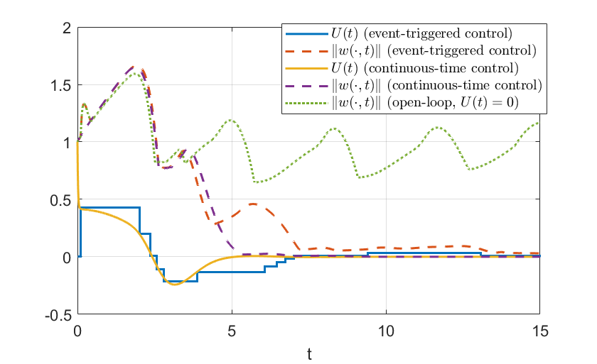
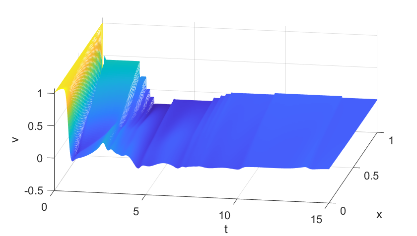
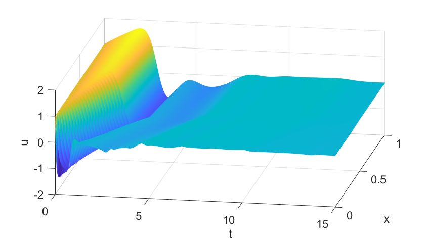
Figure 4: Trajectories of the simulation example.

The performance of the controller is illustrated below within the context of numerical simulations of a system with

$$\lambda^{u}(x) =\begin{cases}0.2&\text{if }x<0.5,\\ 2-x&\text{if }x\geq 0.5,\end{cases},$$ (53)

$$\lambda^{v}(x) =1+0.5\,x,$$ (54)

$$f^{u}((u,v),x) =\frac{1}{3-x}\sin(u+v),$$ (55)

$$f^{v}((u,v),x) =\sin(v-u),$$ (56)

$$g(v,t) =-v,$$ (57)

and initial condition $u_{0}(x)=v_{0}(x)=1$ for all $x\in[0,1]$. The parameters are such that in open-loop with $U(t)=0$ for all $t\geq 0$, the origin is an unstable equilibrium. The simulation and prediction operators are implemented by the method of lines, i.e., semi-discretizing the PDEs in space using first-order finite differences with 50 spatial elements. The resulting high-order ODE is solved in matlab using ode45, where the trigger events are implemented using the odeset(’Events’,$\ldots$) option. The trigger-parameter is chosen as $\varepsilon=\max\{0.05,0.25\,\|w(\cdot,t)\|_{\infty}\}$.

The simulated trajectories are shown in Figure 4. Overall the closed-loop trajectories converge to the origin as expected from the theory. Convergence is slightly slower when the event-triggered controller is used, as compared to the continuous-time implementation where the control input is updated at every time step of the solver, but performance is still very good. One can also see the correlation that there are more trigger times when the continuous control input changes quickly, whereas the control input in the event-triggered version is constant for long periods when the system is close to the origin. In a real-world system this would reduce wear on the actuators significantly.

V Conclusion

We proposed an event-triggered implementation of predictive boundary controllers for semilinear hyperbolic systems. A relatively simple static trigger condition is used. The same trigger-mechanism can also be applied to backstepping control of linear systems, where a less computationally expensive implementation is possible. Compared to other approaches to event-triggered control of hyperbolic PDEs in the literature, no Lyapunov functions are required, which avoids some conservativeness. The approach is also generalizable. For instance, by replacing the state measurement in our event-triggered control scheme with the state estimate obtained via the finite-time convergent boundary observers from [14], one solves the event-triggered output feedback control problem. In quasilinear systems, Lipschitz-continuity of the control inputs is necessary for well-posedness of broad solutions. Therefore, when extending the proposed event-triggered control scheme to quaslinear systems, the transition between different values of $\bar{U}$ needs to be smooth instead of by a jump. Once that transition is completed, the control input can remain constant until the update condition is triggered again.

References

- [1] G. Bastin and J.-M. Coron, Stability and boundary stabilization of 1-d hyperbolic systems. Springer, 2016, vol. 88.
- [2] J. M. Greenberg and T.-T. Li, “The effect of boundary damping for the quasilinear wave equation,” Journal of Differential Equations, vol. 52, no. 1, pp. 66–75, 1984.
- [3] J.-M. Coron, B. d’Andrea Novel, and G. Bastin, “A strict Lyapunov function for boundary control of hyperbolic systems of conservation laws,” IEEE Transactions on Automatic Control, vol. 52, no. 1, pp. 2–11, 2007.
- [4] M. Cirina, “Boundary controllability of nonlinear hyperbolic systems,” SIAM Journal on Control, vol. 7, no. 2, pp. 198–212, 1969.
- [5] T.-T. Li and B.-P. Rao, “Exact boundary controllability for quasi-linear hyperbolic systems,” SIAM Journal on Control and Optimization, vol. 41, no. 6, pp. 1748–1755, 2003.
- [6] R. Vazquez, M. Krstic, and J.-M. Coron, “Backstepping boundary stabilization and state estimation of a 2 2 linear hyperbolic system,” in 2011 50th IEEE CDC and European Control Conference, 2011.
- [7] O. M. Aamo, “Disturbance rejection in linear hyperbolic systems,” IEEE Transactions on Automatic Control, vol. 58, no. 5, pp. 1095–1106, 2013.
- [8] R. Vazquez and M. Krstic, “Bilateral boundary control of one-dimensional first-and second-order PDEs using infinite-dimensional backstepping,” in Decision and Control (CDC), 2016 IEEE 55th Conference on. IEEE, 2016, pp. 537–542.
- [9] J. Auriol and F. Di Meglio, “Two-sided boundary stabilization of two linear hyperbolic PDEs in minimum time,” in Decision and Control (CDC), 2016 IEEE 55th Conference on. IEEE, 2016, pp. 3118–3124.
- [10] J. Deutscher, “Finite-time output regulation for linear 2 2 hyperbolic systems using backstepping,” Automatica, vol. 75, pp. 54–62, 2017.
- [11] J. Auriol and F. Di Meglio, “Minimum time control of heterodirectional linear coupled hyperbolic PDEs,” Automatica, vol. 71, pp. 300–307, 2016.
- [12] F. Di Meglio, F. B. Argomedo, L. Hu, and M. Krstic, “Stabilization of coupled linear heterodirectional hyperbolic pde–ode systems,” Automatica, vol. 87, pp. 281–289, 2018.
- [13] J. Auriol, “Output feedback stabilization of an underactuated cascade network of interconnected linear PDE systems using a backstepping approach,” Automatica, vol. 117, p. 108964, 2020.
- [14] T. Strecker and O. M. Aamo, “Output feedback boundary control of semilinear hyperbolic systems,” Automatica, vol. 83, pp. 290–302, 2017.
- [15] ——, “Output feedback boundary control of series interconnections of semilinear hyperbolic systems,” in 20th IFAC World Congress, 2017. IFAC, 2017.
- [16] ——, “Two-sided boundary control and state estimation of semilinear hyperbolic systems,” in 2017 IEEE 56th Annual Conference on Decision and Control (CDC). IEEE, 2017, pp. 2511–2518.
- [17] T. Strecker, O. M. Aamo, and M. Cantoni, “Boundary feedback control of 2x2 quasilinear hyperbolic systems: Predictive synthesis and robustness analysis,” IEEE Transactions on Automatic Control, 2021.
- [18] ——, “Predictive feedback boundary control of semilinear and quasilinear hyperbolic PDE-ODE systems,” accepted to Automatica; https://arxiv.org/abs/2105.09039, 2022.
- [19] N. Espitia, A. Girard, N. Marchand, and C. Prieur, “Event-based boundary control of a linear hyperbolic system via backstepping approach,” IEEE Transactions on Automatic Control, vol. 63, no. 8, pp. 2686–2693, 2017.
- [20] N. Espitia, “Observer-based event-triggered boundary control of a linear 2 2 hyperbolic systems,” Systems & Control Letters, vol. 138, p. 104668, 2020.
- [21] J. Wang and M. Krstic, “Adaptive event-triggered pde control for load-moving cable systems,” Automatica, vol. 129, p. 109637, 2021.
- [22] ——, “Event-triggered backstepping control of 2 2 hyperbolic pde-ode systems,” IFAC-PapersOnLine, vol. 53, no. 2, pp. 7551–7556, 2020.
- [23] M. A. Davó, D. Bresch-Pietri, C. Prieur, and F. Di Meglio, “Stability analysis of a linear hyperbolic system with a sampled-data controller via backstepping method and looped-functionals,” IEEE Transactions on Automatic Control, vol. 64, no. 4, pp. 1718–1725, 2018.
- [24] W. P. Heemels, K. H. Johansson, and P. Tabuada, “An introduction to event-triggered and self-triggered control,” in 51st conference on decision and control. IEEE, 2012.
- [25] F. Di Meglio, R. Vazquez, and M. Krstic, “Stabilization of a system of coupled first-order hyperbolic linear PDEs with a single boundary input,” IEEE Transactions on Automatic Control, vol. 58, no. 12, pp. 3097–3111, 2013.
- [26] A. Bressan, Hyperbolic systems of conservation laws: the one-dimensional Cauchy problem. Oxford University Press, 2000, vol. 20.
- [27] T.-T. Li, B. Rao, and Y. Jin, “Semi-global solution and exact boundary controllability for reducible quasilinear hyperbolic systems,” ESAIM: Mathematical Modelling and Numerical Analysis, vol. 34, no. 2, pp. 399–408, 2000.