Three-dimensional third-order gas-kinetic scheme on hybrid unstructured meshes for Euler and Navier-Stokes equations

Abstract

In this paper, a third-order gas-kinetic scheme is developed on the three-dimensional hybrid unstructured meshes for the numerical simulation of compressible inviscid and viscous flows. In the classical weighted essentially non-oscillatory (WENO) scheme, the high-order spatial accuracy is achieved by the non-linear combination of lower order polynomials. However, for the hybrid unstructured meshes, the procedures, including the selection of candidate stencils and calculation of linear weights, become extremely complicated, especially for three-dimensional problems. To overcome the drawbacks, a third-order WENO reconstruction is developed on the hybrid unstructured meshes, including tetrahedron, pyramid, prism and hexahedron. A simple strategy is adopted for the selection of big stencil and sub-stencils, and the topologically independent linear weights are used in the spatial reconstruction. A unified interpolation is used for the volume integral of different control volumes, as well as the flux integration over different cell interfaces. Incorporate with the two-stage fourth-order temporal discretization, the explicit high-order gas-kinetic schemes are developed for unsteady problems. With the lower-upper symmetric Gauss-Seidel (LU-SGS) methods, the implicit high-order gas-kinetic schemes are developed for steady problems. A variety of numerical examples, from the subsonic to supersonic flows, are presented to validate the accuracy and robustness for both inviscid and viscous flows. To accelerate the computation, the current scheme is implemented with the graphics processing unit (GPU) using compute unified device architecture (CUDA). The speedup of GPU code suggests the potential of high-order gas-kinetic schemes for the large scale computation.

1 Introduction

The unstructured meshes are widely used in the computational fluid dynamics (CFD) methods with complex geometries. Various high-order numerical methods on unstructured meshes have been developed in the past decades, including discontinuous Galerkin (DG) DG-A ; DG-B ; DG-C , spectral volume (SV) SV-A , correction procedure using reconstruction (CPR) CPR-A , the finite-volume type essential non-oscillatory (ENO) ENO-un , weighted essential non-oscillatory (WENO) WENO-un1 ; WENO-un2 ; WENO-un3 ; WENO-un4 and Hermite WENO (HWENO) HWENO methods.

In the framework of finite volume methods, the WENO schemes have been successfully developed for the compressible flows, the WENO-type high-order methods have received the most attention in recent years. For the one-dimensional WENO schemes WENO-Liu ; WENO-JS ; WENO-Z , the high-order of accuracy is obtained by the non-linear combination of lower order polynomials from the candidate stencils. For the multi-dimensional structured meshes, the WENO scheme is performed dimension-by-dimension. On the two-dimensional unstructured meshes, the WENO schemes were also developed with same idea WENO-un1 ; WENO-un2 ; WENO-un3 . However, the linear weights need to be computed and restored for each cell, and the appearance of negative weights also affect the performance of WENO schemes. The central/compact WENO (CWENO) schemes were developed when facing distorted local mesh geometries or degenerate cases CWENO1 ; CWENO2 ; CWENO3 . Following the original idea of classical CWENO schemes, two types of WENO scheme is developed, i.e., the WENO schemes with adaptive order WENO-ao-1 ; WENO-ao-2 and the simple WENO schemes WENO-simple-1 ; WENO-simple-2 . The linear weights are topology independent and artificially set to be positive numbers, and the non-linear weights are chosen to achieve the optimal order of accuracy in the smooth region and suppress the oscillations near the discontinuous region. Most of efforts are spent in the unstructured triangular meshes for two-dimensional problems and tetrahedral meshes for three-dimensional problems. However, in practical applications, such as the viscous flows around or inside complex geometries, the hybrid unstructured meshes are usually adopted for accuracy and efficiency. More recently, the WENO schemes on arbitrary unstructured meshes has been developed for inviscid flows WENO-un4 ; WENO-un5 ; WENO-un6 , and also extended for viscous flows, including laminar, transitional and turbulent problems WENO-un7 .

In the past decades, the gas-kinetic schemes (GKS) based on the Bhatnagar-Gross-Krook (BGK) model BGK-1 ; BGK-2 have been developed systematically for the computations from low speed flows to supersonic ones GKS-Xu1 ; GKS-Xu2 . The gas-kinetic scheme presents a gas evolution process from the kinetic scale to hydrodynamic scale, and both inviscid and viscous fluxes can be calculated in one framework. Recently, a time-dependent gas distribution function can be constructed at a cell interface, which is important for the construction of high-order scheme. With the two-stage temporal discretization, which was originally developed for the Lax-Wendroff type flow solvers GRP-high-1 ; GRP-high-2 , a reliable framework was provided to construct gas-kinetic scheme with fourth-order and even higher-order temporal accuracy GKS-high-1 ; GKS-high-2 . More importantly, the high-order scheme is as robust as the second-order one and works perfectly from the subsonic to hypersonic flows. The implicit methods for GKS and unified GKS have also been constructed GKS-implicit-1 ; GKS-implicit-2 , and the implicit temporal methods provide efficient techniques for speeding up the convergence of steady problems. Recently, with the simple WENO type reconstruction, the third-order and fourth-order gas-kinetic schemes are developed on the three-dimensional structured meshes, in which a simple strategy of selecting stencils for reconstruction is adopted and the topology independent linear weights are used GKS-high-4 ; GKS-high-5 . Based on the spatial and temporal coupled property of GKS solver and the HWENO reconstruction HWENO , the high-order compact gas-kinetic schemes are also developed GKS-high-6 ; GKS-high-7 .

In this paper, a third-order gas-kinetic scheme is developed on the three-dimensional hybrid unstructured meshes for the compressible inviscid and viscous flows. Due to the complex mesh topology of hybrid unstructured meshes, the procedures of classical WENO scheme, including the selection of candidate stencils and calculation of linear weights, become extremely complicated. A simple WENO reconstruction is extended to the unstructured meshes with tetrahedral, pyramidal, prismatic and hexahedral cells. A large stencil is selected with the neighboring cells and the neighboring cells of neighboring cells, and a quadratic polynomial can be obtained. For the tetrahedral and pyramidal cells, the centroids of control volume and neighboring cells might be coplanar, and the coefficient matrix might become singular. A robust selections of candidate sub-stencils are also given, such that the linear polynomials are solvable for each sub-stencil. The trilinear interpolation is used for each cell, and the Gaussian quadrature over a plane cell interface is used to achieve the spatial accuracy. For the cell interface, the trilinear interpolation degenerates to a bilinear interpolation, and a unified formulation can be used to calculate the numerical fluxes over both triangular and quadrilateral interfaces. Incorporate with the two-stage fourth-order temporal discretization, the explicit high-order gas-kinetic schemes are developed for unsteady problems. With the lower-upper symmetric Gauss-Seidel (LU-SGS) methods, the implicit high-order gas-kinetic schemes are developed for steady problems. Various three-dimensional numerical experiments, including unsteady and steady problems, are presented to to validate the accuracy and robustness of WENO scheme. To accelerate the computation, the current scheme is implemented to run on graphics processing unit (GPU) using compute unified device architecture (CUDA). The computational efficiency using single Nvidia TITAN RTX GPU is demonstrated. Obtained results are compared with those obtained by an octa-core Intel i7-11700 CPU in terms of calculation time. Compared with the CPU code, 6x speedup is achieved for GPU code. In the future, more challenging compressible flow problems will be investigated with multiple GPUs.

This paper is organized as follows. In Section 2, the three-dimensional WENO reconstruction on the hybrid unstructured meshes will be introduced. The high-order gas-kinetic scheme for inviscid and viscous flows will be presented in Section 3. Numerical examples are included in Section 4. The last section is the conclusion.

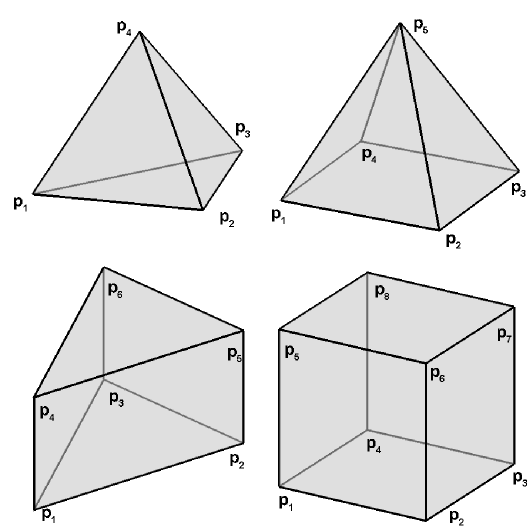
Figure 1: Schematic for tetrahedron, pyramid, prism and hexahedron.

2 WENO reconstruction on hybrid unstructured meshes

In this section, a third-order WENO reconstruction will be presented on the three-dimensional unstructured hybrid meshes. Similar with the previous study, the idea of simple WENO reconstruction is adopted WENO-simple-1 ; WENO-simple-2 ; GKS-high-5 ; GKS-high-4 . For the unstructured hybrid meshes, the meshes are consist of the tetrahedral, pyramidal, prismatic and hexahedral cells. The schematic of the cells are given in Fig.1 with the label of vertexes. For the sake of clearness, the faces of control volume also need to be labeled. For the cell $\Omega_{0}$, the faces are labeled as follows

• For the tetrahedral cell, four faces are denoted as

  $$F_{1}=\{p_{1}p_{2}p_{3}\},F_{2}=\{p_{1}p_{2}p_{4}\},F_{3}=\{p_{2}p_{3}p_{4}\},F_{4}=\{p_{3}p_{1}p_{4}\}.$$

• For the pyramidal cell, five faces are denoted as

  $$F_{1}=\{p_{1}p_{2}p_{5}\},F_{2}=\{p_{2}p_{3}p_{5}\},F_{3}=\{p_{3}p_{4}p_{5}\},F_{4}=\{p_{4}p_{1}p_{5}\},F_{5}=\{p_{1}p_{2}p_{3}p_{4}\}.$$

• For the prismatic cell, five faces are denoted as

  $$F_{1}=\{p_{1}p_{2}p_{3}\},F_{2}=\{p_{4}p_{5}p_{6}\},F_{3}=\{p_{1}p_{2}p_{6}p_{4}\},F_{4}=\{p_{2}p_{3}p_{6}p_{5}\},F_{5}=\{p_{3}p_{1}p_{4}p_{6}\}.$$

• For the hexahedral cell, six faces are denoted as

  $$F_{1}=\{p_{1}p_{2}p_{3}p_{4}\},F_{2}=\{p_{1}p_{2}p_{6}p_{5}\},F_{3}=\{p_{2}p_{3}p_{7}p_{6}\},$$

  $$F_{4}=\{p_{3}p_{4}p_{8}p_{7}\},F_{5}=\{p_{4}p_{1}p_{5}p_{8}\},F_{6}=\{p_{5}p_{6}p_{7}p_{8}\}.$$

With the labeled faces given above, the neighboring cell of $\Omega_{i}$, which shares the face $F_{p}$, is denoted as $\Omega_{i_{p}}$. Meanwhile, the neighboring cells of $\Omega_{i_{p}}$ are denoted as $\Omega_{i_{pm}}$. To achieve the third-order accuracy, a big stencil $S_{i}$ for cell $\Omega_{i}$ is selected as follows

$$S_{i} =\{\Omega_{i},\Omega_{i_{p}},\Omega_{i_{pm}}\},$$

which is consist of the neighboring cells and neighboring cells of neighboring cells of $\Omega_{i}$.

Taking the boundary condition into account, the selection of big stencil becomes more complicated. In the following, the inner cell represents the cell with no face on the boundary and the boundary cell is the cell with at least one face on the boundary. For the periodic boundary condition, the generated triangular or quadrilateral meshes on the periodic boundaries should be identical. If $\Omega_{i}$ is boundary cell, the neighboring cells of $\Omega_{i}$ can be found with the periodic boundary condition. Thus, for each cell $\Omega_{i}$ in the domain, the big stencil $S_{i}$ can be selected. For other boundary conditions, the following two stages need to be considered. If $\Omega_{i}$ is an inner cell and $\Omega_{i_{p}}$ is a boundary cell, the geometric information of $\Omega_{i_{pm}}$ can be provided according to the mirror image for cell interface and the flow variables are given according to the boundary condition. If $\Omega_{i}$ is a boundary cell, the geometric information and flow variables of the ghost cell $\Omega_{i_{p}}$ are provided firstly. For the ghost cell $\Omega_{i_{p}}$, the geometric information of its neighboring cells $\Omega_{i_{pm}}$ are provided by the mirror image of neighboring cells of $\Omega_{i}$, and the flow variables on the cell $\Omega_{i_{pm}}$ are given according to the boundary condition corresponding to neighboring cells of $\Omega_{i}$.

With the procedure above, the candidate stencils can be selected and the index of big stencil is rearranged as

$$S_{i}=\{\Omega_{0},\Omega_{1},...,\Omega_{N},\Omega_{N+1},...,\Omega_{K}\},$$

where $K$ is the total number of cells and $N$ is the number of neighboring cells. Based on the big stencil, a quadratic polynomial can be constructed as

$$P_{0}(\bm{x})=Q_{0}+\sum_{|\bm{n}|=1}^{2}a_{\bm{n}}p_{\bm{n}}(\bm{x}),$$

where $Q_{0}$ is the cell averaged conservative variables over $\Omega_{0}$, the multi-index $\bm{n}=(n_{1},n_{2},n_{3})$ and $|\bm{n}|=n_{1}+n_{2}+n_{3}$. The base function $p_{\bm{n}}(\bm{x})$ is defined as

$$\displaystyle p_{\bm{n}}(\bm{x})=x^{n_{1}}y^{n_{2}}z^{n_{3}}-\frac{1}{\left|\Omega_{0}\right|}\iiint_{\Omega_{0}}x^{n_{1}}y^{n_{2}}z^{n_{3}}\text{d}V.$$

To determine this polynomial, the following constrains need to be satisfied for all cells in the big stencil

$$\frac{1}{\left|\Omega_{k}\right|}\iiint_{\Omega_{k}}P_{0}(\bm{x})\text{d}V=Q_{k},~{}\Omega_{k}\in S,$$

where $Q_{k}$ is the conservative variable with newly rearranged index. An over-determined linear system can be generated and the least square method is used to obtain the coefficients.

To deal with the discontinuity, the linear polynomials are constructed based on the candidate sub-stencils

$$P_{m}(\bm{x})=Q_{0}+\sum_{|\bm{n}|=1}b_{\bm{n}}^{m}p_{\bm{n}}(\bm{x}),$$ (1)

where $m=1,...M$ and $M$ is the number of sub-stencils. To determine these polynomials, the following constrains need to be satisfied

$$\frac{1}{\left|\Omega_{m_{k}}\right|}\iiint_{\Omega_{k}}P_{m}(\bm{x})\text{d}V=Q_{k},~{}\Omega_{m_{k}}\in S_{i_{m}},$$

where $Q_{m_{k}}$ is the conservative variable with newly rearranged index. With the selected sub-stencils $S_{i_{m}}$, the the linear polynomials can be fully determined.

• For the hexahedral cell, $M=8$ and the sub-candidate stencils are selected as follows

  $$S_{i_{1}}=\{\Omega_{i},\Omega_{i_{1}},\Omega_{i_{2}},\Omega_{i_{3}}\},~{}S_{i_{5}}=\{\Omega_{i},\Omega_{i_{6}},\Omega_{i_{2}},\Omega_{i_{3}}\},$$

  $$S_{i_{2}}=\{\Omega_{i},\Omega_{i_{1}},\Omega_{i_{3}},\Omega_{i_{4}}\},~{}S_{i_{6}}=\{\Omega_{i},\Omega_{i_{6}},\Omega_{i_{3}},\Omega_{i_{4}}\},$$

  $$S_{i_{3}}=\{\Omega_{i},\Omega_{i_{1}},\Omega_{i_{4}},\Omega_{i_{5}}\},~{}S_{i_{7}}=\{\Omega_{i},\Omega_{i_{6}},\Omega_{i_{4}},\Omega_{i_{5}}\},$$

  $$S_{i_{4}}=\{\Omega_{i},\Omega_{i_{1}},\Omega_{i_{5}},\Omega_{i_{2}}\},~{}S_{i_{8}}=\{\Omega_{i},\Omega_{i_{6}},\Omega_{i_{5}},\Omega_{i_{2}}\}.$$

• For the prismatic cell, $M=6$ and the sub-candidate stencils are selected as

  $$S_{i_{1}}=\{\Omega_{i},\Omega_{i_{1}},\Omega_{i_{3}},\Omega_{i_{4}}\},~{}S_{i_{4}}=\{\Omega_{i},\Omega_{i_{2}},\Omega_{i_{3}},\Omega_{i_{4}}\},$$

  $$S_{i_{2}}=\{\Omega_{i},\Omega_{i_{1}},\Omega_{i_{4}},\Omega_{i_{5}}\},~{}S_{i_{5}}=\{\Omega_{i},\Omega_{i_{2}},\Omega_{i_{4}},\Omega_{i_{5}}\},$$

  $$S_{i_{3}}=\{\Omega_{i},\Omega_{i_{1}},\Omega_{i_{5}},\Omega_{i_{3}}\},~{}S_{i_{6}}=\{\Omega_{i},\Omega_{i_{2}},\Omega_{i_{5}},\Omega_{i_{3}}\}.$$

For the hexahedral and pyramidal cells, the sub-stencils are consist of $\Omega_{0}$ and three neighboring cells. The linear polynomials can be determined.

However, for the tetrahedral and pyramidal cells, the centroids of $\Omega_{0}$ and three of neighboring cells might becomes coplanar. If we only use the neighboring cells for the sub-candidate stencils, the coefficient matrix might become singular and more cells are needed.

• For the tetrahedral cell, $M=4$ and the sub-candidate stencils are selected as

  $$S_{i_{1}}=\{\Omega_{i},\Omega_{i_{1}},\Omega_{i_{2}},\Omega_{i_{3}},\Omega_{i_{11}},\Omega_{i_{12}},\Omega_{i_{13}}\},$$

  $$S_{i_{2}}=\{\Omega_{i},\Omega_{i_{1}},\Omega_{i_{2}},\Omega_{i_{4}},\Omega_{i_{21}},\Omega_{i_{22}},\Omega_{i_{23}}\},$$

  $$S_{i_{3}}=\{\Omega_{i},\Omega_{i_{2}},\Omega_{i_{3}},\Omega_{i_{4}},\Omega_{i_{31}},\Omega_{i_{32}},\Omega_{i_{33}}\},$$

  $$S_{i_{4}}=\{\Omega_{i},\Omega_{i_{3}},\Omega_{i_{1}},\Omega_{i_{4}},\Omega_{i_{41}},\Omega_{i_{42}},\Omega_{i_{43}}\}.$$

• For the pyramidal cell, $M=8$ and the sub-candidate stencils are selected as

  $$S_{i_{1}} =\{\Omega_{i},\Omega_{i_{1}},\Omega_{i_{2}},\Omega_{i_{3}},\Omega_{i_{11}},\Omega_{i_{12}},\Omega_{i_{13}}\},~{}S_{i_{5}}=\{\Omega_{i},\Omega_{i_{1}},\Omega_{i_{2}},\Omega_{i_{5}},\Omega_{i_{11}},\Omega_{i_{12}},\Omega_{i_{13}}\},$$

  $$S_{i_{2}} =\{\Omega_{i},\Omega_{i_{2}},\Omega_{i_{3}},\Omega_{i_{4}},\Omega_{i_{21}},\Omega_{i_{22}},\Omega_{i_{23}}\},~{}S_{i_{6}}=\{\Omega_{i},\Omega_{i_{2}},\Omega_{i_{3}},\Omega_{i_{5}},\Omega_{i_{21}},\Omega_{i_{22}},\Omega_{i_{23}}\},$$

  $$S_{i_{3}} =\{\Omega_{i},\Omega_{i_{3}},\Omega_{i_{4}},\Omega_{i_{1}},\Omega_{i_{31}},\Omega_{i_{32}},\Omega_{i_{33}}\},~{}S_{i_{7}}=\{\Omega_{i},\Omega_{i_{3}},\Omega_{i_{4}},\Omega_{i_{5}},\Omega_{i_{31}},\Omega_{i_{32}},\Omega_{i_{33}}\},$$

  $$S_{i_{4}} =\{\Omega_{i},\Omega_{i_{4}},\Omega_{i_{1}},\Omega_{i_{2}},\Omega_{i_{41}},\Omega_{i_{42}},\Omega_{i_{43}}\},~{}S_{i_{8}}=\{\Omega_{i},\Omega_{i_{4}},\Omega_{i_{1}},\Omega_{i_{5}},\Omega_{i_{41}},\Omega_{i_{42}},\Omega_{i_{43}}\}.$$

where $\Omega_{i_{pm}}\neq\Omega_{i},p=1,2,3,4,m=1,2,3$, and the cells of sub-candidate stencils are consist of the three neighboring cells and three neighboring cells of one neighboring cell. With such an enlarged sub-stencils, Eq.(1) becomes solvable and the linear polynomials can be determined.

With the reconstructed polynomial $P_{m}(\bm{x}),m=0,...,M$, the point-value $Q(\bm{x}_{G})$ and the spatial derivatives $\partial_{x,y,z}Q(\bm{x}_{G})$ for reconstructed variables at Gaussian quadrature point can be given by the non-linear combination

$$\begin{split}Q(\bm{x}_{G})=\overline{\omega}_{0}(\frac{1}{\gamma_{0}}P_{0}(\bm{x}_{G})-&\sum_{m=1}^{M}\frac{\gamma_{m}}{\gamma_{0}}P_{m}(\bm{x}_{G}))+\sum_{m=1}^{M}\overline{\omega}_{m}P_{m}(\bm{x}_{G}),\\ \partial_{x,y,z}Q(\bm{x}_{G})=\overline{\omega}_{0}(\frac{1}{\gamma_{0}}\partial_{x,y,z}P_{0}(\bm{x}_{G})-&\sum_{m=1}^{M}\frac{\gamma_{m}}{\gamma_{0}}\partial_{x,y,z}P_{m}(\bm{x}_{G}))+\sum_{m=1}^{M}\overline{\omega}_{m}\partial_{x,y,z}P_{m}(\bm{x}_{G})),\end{split}$$ (2)

where $\gamma_{0},\gamma_{1},...,\gamma_{M}$ are the linear weights. In the computation, $\gamma_{i}=0.0125,i=1,...,M$ and $\gamma_{0}=1-0.0125M$. $\partial_{x,y,z}P_{m}(\bm{x}_{G})$ can be obtained by taking derivatives of the candidate polynomials directly. The non-linear weights $\omega_{m}$ and normalized non-linear weights $\overline{\omega}_{m}$ are defined as

$$\overline{\omega}_{m}=\frac{\omega_{m}}{\sum_{m=0}^{M}\omega_{m}},~{}\omega_{m}=\gamma_{m}\Big{[}1+\Big{(}\frac{\tau}{\beta_{m}+\epsilon}\Big{)}\Big{]},$$

where $\epsilon$ is a small positive number. To achieve a third-order accuracy, a quadratic polynomial is used for $P_{0}(\bm{x})$ and $\tau$ is chosen as

$$\tau=\sum_{m=1}^{M}\Big{(}\frac{|\beta_{0}-\beta_{m}|}{M}\Big{)}.$$

The smooth indicator $\beta_{m}$ is defined as

$$\beta_{m}=\sum_{|l|=1}^{r_{m}}|\Omega_{ijk}|^{\frac{2|l|}{3}-1}\int_{\Omega_{ijk}}\Big{(}\frac{\partial^{l}P_{m}}{\partial_{x}^{l_{1}}\partial_{y}^{l_{2}}\partial_{z}^{l_{3}}}(x,y,z)\Big{)}^{2}\text{d}V,$$ (3)

where $r_{0}=2$ and $r_{m}=1$ for $m=1,...,M$. It can be proved that Eq.(2) ensures third-order accuracy and more details can be found in GKS-high-4 .

For the spatial reconstruction, the integrals over tetrahedron, pyramid, prism and hexahedron, including volume of cell, need to be calculated. The volume of tetrahedron can be given by an explicit formulation. The pyramid, prism and hexahedron can be divided into several tetrahedrons, and their integrals can be calculated simply. However, the quadrilateral interface of pyramid, prism and hexahedron maybe non-coplanar, such kind of method for calculating volume is inaccurate. For the sake of accuracy, the integrals over a hexahedron cell is computed by the Gaussian quadrature

$$\iiint_{\Omega}x^{a}y^{b}z^{c}\text{d}x\text{d}y\text{d}z=\sum_{l,m,n=1}^{3}\omega_{lmn}x^{a}y^{b}z^{c}(\xi_{l},\eta_{m},\zeta_{n})\Big{|}\frac{\partial(x,y,z)}{\partial(\xi,\eta,\zeta)}\Big{|}_{(\xi_{l},\eta_{m},\zeta_{n})}\Delta\xi\Delta\eta\Delta\zeta,$$

where $\omega_{lmn}$ is the Gaussian quadrature weight and $(\xi_{l},\eta_{m},\zeta_{n})$ is the quadrature point. A trilinear interpolation is introduced to parameterize the hexahedron cell $\Omega_{i}$

$$\bm{X}(\xi,\eta,\zeta)=\sum_{m=1}^{8}\bm{x}_{m}\psi_{m}(\xi,\eta,\zeta),$$ (4)

where $(\xi,\eta,\zeta)\in[-1/2,1/2]^{3}$, $\bm{x}_{m}$ is the vertex of a hexahedron cell and the base function $\psi_{m}$ is given as follows

$$\psi_{1}=\frac{1}{8}(1-2\xi)(1-2\eta)(1-2\zeta),\psi_{2}=\frac{1}{8}(1-2\xi)(1-2\eta)(1+2\zeta),$$

$$\psi_{3}=\frac{1}{8}(1-2\xi)(1+2\eta)(1-2\zeta),\psi_{4}=\frac{1}{8}(1-2\xi)(1+2\eta)(1+2\zeta),$$

$$\psi_{5}=\frac{1}{8}(1+2\xi)(1-2\eta)(1-2\zeta),\psi_{6}=\frac{1}{8}(1+2\xi)(1-2\eta)(1+2\zeta),$$

$$\psi_{7}=\frac{1}{8}(1+2\xi)(1+2\eta)(1-2\zeta),\psi_{8}=\frac{1}{8}(1+2\xi)(1+2\eta)(1+2\zeta).$$

With trilinear interpolation Eq.(4), the hexahedron cell with non-coplanar vertexes can be dealt with accurately. As shown in Fig.1, the hexahedron cell denoted as the sequential label $\Omega=\{p_{1}p_{2}p_{3}p_{4}p_{5}p_{6}p_{7}p_{8}\}$. For the tetrahedral, pyramidal and prismatic cells, they can be considered as degenerated hexahedron, and can be relabeled follows

$$\Omega =\{p_{1}p_{2}p_{3}p_{3}p_{4}p_{4}p_{4}p_{4}\}\text{~{}for tetrahedron},$$

$$\Omega =\{p_{1}p_{2}p_{3}p_{4}p_{5}p_{5}p_{5}p_{5}\}\text{~{}for pyramid},$$

$$\Omega =\{p_{1}p_{2}p_{3}p_{3}p_{4}p_{5}p_{6}p_{6}\}\text{~{}for prism}.$$

Eq.(4) is also used to parameter the tetrahedral, pyramidal, prismatic cells and the integrals can be calculated.

3 High-order gas-kinetic scheme

3.1 BGK equation and finite volume scheme

With the thrid-order WENO reconstruction, the high-order gas-kinetic scheme (HGKS) will be presented for the three-dimensional flows in the finite volume framework. The three-dimensional BGK equation BGK-1 ; BGK-2 can be written as

$$f_{t}+uf_{x}+vf_{y}+wf_{z}=\frac{g-f}{\tau},$$ (5)

where $\bm{u}=(u,v,w)$ is the particle velocity, $f$ is the gas distribution function, $g$ is the three-dimensional Maxwellian distribution and $\tau$ is the collision time. The collision term satisfies the compatibility condition

$$\int\frac{g-f}{\tau}\psi\text{d}\Xi=0,$$ (6)

where $\displaystyle\psi=(\psi_{1},...,\psi_{5})^{T}=(1,u,v,w,\frac{1}{2}(u^{2}+v^{2}+w^{2}+\varsigma^{2}))^{T}$, the internal variables $\varsigma^{2}=\varsigma_{1}^{2}+...+\varsigma_{K}^{2}$, $\text{d}\Xi=\text{d}u\text{d}v\text{d}w\text{d}\varsigma^{1}...\text{d}\varsigma^{K}$, $\gamma$ is the specific heat ratio and $K=(5-3\gamma)/(\gamma-1)$ is the degrees of freedom for three-dimensional flows. According to the Chapman-Enskog expansion for BGK equation, the macroscopic governing equations can be derived GKS-Xu1 ; GKS-Xu2 . In the continuum region, the BGK equation can be rearranged and the gas distribution function can be expanded as

$$f=g-\tau D_{\bm{u}}g+\tau D_{\bm{u}}(\tau D_{\bm{u}})g-\tau D_{\bm{u}}[\tau D_{\bm{u}}(\tau D_{\bm{u}})g]+...,$$

where $D_{\bm{u}}=\displaystyle\frac{\partial}{\partial t}+\bm{u}\cdot\nabla$. With the zeroth-order truncation $f=g$, the Euler equations can be obtained. For the first-order truncation

$$f=g-\tau(ug_{x}+vg_{y}+wg_{z}+g_{t}),$$

the Navier-Stokes equations can be obtained GKS-Xu1 ; GKS-Xu2 .

Taking moments of Eq.(5) and integrating with respect to space, the semi-discretized finite volume scheme can be expressed as

$$\frac{\partial Q_{i}}{\partial t}=\mathcal{L}(Q_{i}),$$ (7)

where $Q=(\rho,\rho U,\rho V,\rho W,\rho E)$ is the cell averaged conservative value of $\Omega_{i}$. The operator $\mathcal{L}$ is defined as

$$\mathcal{L}(Q_{i})=-\frac{1}{|\Omega_{i}|}\sum_{i_{p}\in N(i)}\mathbb{F}_{i_{p}}(t)=-\frac{1}{|\Omega_{i}|}\sum_{i_{p}\in N(i)}\iint_{\Sigma_{i_{p}}}\bm{F}(Q,t)\text{d}\sigma,$$ (8)

where $Q_{i}$ is the cell averaged conservative variables of $\Omega_{i}$, $|\Omega_{i}|$ is the area of $\Omega_{i}$, $\Sigma_{i_{p}}$ is the common cell interface of $\Omega_{i}$ and $\Omega_{i_{p}}$ and $N(i)$ is the set of index for neighbor cells of $\Omega_{i}$.

For the hybrid meshes, the cell interface can be quadrilateral and triangular. The triangular interface can be considered as degenerated quadrilateral interface, where two vertexes of quadrilateral are identical. Thus, both triangular and quadrilateral interfaces can be calculated in a unified formulation. For the quadrilateral interface, the four vertexes may be non-coplanar. To calculate the numerical fluxes accurately, a curved interface need to be considered. To be consist with the calculation of integrals over control volume, a bilinear interpolation is used to parameterize the cell interface as follows

$$\bm{X}(\eta,\zeta)=\sum_{m=1}^{4}\bm{x}_{m}\phi_{m}(\eta,\zeta),$$

where $(\eta,\zeta)\in[-1/2,1/2]^{2}$, $\bm{x}_{m}$ is the vertex of the interface and $\phi_{m}$ is the base function

$$\phi_{1}=\frac{1}{4}(1-2\eta)(1-2\zeta),\phi_{2}=\frac{1}{4}(1-2\eta)(1+2\zeta),$$

$$\phi_{3}=\frac{1}{4}(1+2\eta)(1-2\zeta),\phi_{4}=\frac{1}{4}(1+2\eta)(1+2\zeta),$$

which is a degenerated form of trilinear interpolation Eq.(4). With the parameterized cell interface, the numerical flux can be determined by the following Gaussian integration

$$\mathbb{F}_{i_{p}}(t) =\iint_{\Sigma_{i_{p}}}F(Q,t)\text{d}\sigma=\iint_{\sigma_{i_{p}}}F(Q(\bm{X}(\eta,\zeta)),t)\|\bm{X}_{\eta}\times\bm{X}_{\zeta}\|\text{d}\eta\text{d}\zeta$$

$$=\sum_{k=1}^{4}\omega_{G_{k}}F_{G_{k}}(t)\|\bm{X}_{\eta}\times\bm{X}_{\zeta}\|_{G_{k}}\Delta\eta\Delta\zeta,$$ (9)

where the local orthogonal coordinate for Gaussian quadrature point of the parameterized cell interface is distinct, $\sigma_{i_{p}}=[-1/2,1/2]\times[-1/2,1/2]$, $\omega_{G_{k}}=1/4$ is quadrature weight for Gaussian quadrature point $\bm{x}_{G_{k}},k=1,2,3,4$ and $\bm{x}_{G_{k}}=(\pm\sqrt{3}/3,\pm\sqrt{3}/3)$. The numerical flux at Gaussian quadrature point $F_{G_{k}}(t)$ can be obtained by taking moments of gas distribution function in the global coordinate

$$F_{G_{k}}(t)=\int\bm{\psi}\bm{u}\cdot(\bm{n}_{1})_{G_{k}}f(\bm{x}_{G_{k}},t,\bm{u},\varsigma)\text{d}\Xi,$$ (10)

where $F_{G_{k}}=(F^{\rho}_{G_{k}},F^{\rho U}_{G_{k}},F^{\rho V}_{G_{k}},F^{\rho W}_{G_{k}},F^{\rho E}_{G_{k}})$ and $(\bm{n}_{1})_{G_{k}}$ is the local normal direction.

3.2 Gas-kinetic solver

In the computation, the numerical flux is usually obtained by taking moments of gas distribution function in the local coordinate and transferred to the global coordinate. In the local coordinate, the gas distribution function is constructed by the integral solution of BGK equation Eq.(5)

$$f(\bm{x}_{G_{k}},t,\bm{u},\varsigma)= \frac{1}{\tau}\int_{0}^{t}g(\bm{x}^{\prime},t^{\prime},\bm{u},\varsigma)e^{-(t-t^{\prime})/\tau}\text{d}t^{\prime}+e^{-t/\tau}f_{0}(-\bm{u}t,\varsigma),$$

where the gas distribution function in the local coordinate is also denoted as $f(\bm{x}_{G_{k}},t,\bm{u},\varsigma)$ for simplicity, $\bm{u}=(u,v,w)$ is the particle velocity in the local coordinate, $\bm{x}_{G_{k}}=\bm{x}^{\prime}+\bm{u}(t-t^{\prime})$ is the trajectory of particles, $f_{0}$ is the initial gas distribution function, and $g$ is the corresponding equilibrium state. With the reconstruction of macroscopic variables, the second-order gas distribution function at the cell interface can be expressed as

$$\begin{split}f(\bm{x}_{G_{k}},t,\bm{u},\varsigma)&=(1-e^{-t/\tau})g_{0}+((t+\tau)e^{-t/\tau}-\tau)(\overline{a}_{1}u+\overline{a}_{2}v+\overline{a}_{3}w)g_{0}\\ &+(t-\tau+\tau e^{-t/\tau}){\bar{A}}g_{0}\\ &+e^{-t/\tau}g_{r}[1-(\tau+t)(a_{1}^{r}u+a_{2}^{r}v+a_{3}^{r}w)-\tau A^{r})](1-H(u))\\ &+e^{-t/\tau}g_{l}[1-(\tau+t)(a_{1}^{l}u+a_{2}^{l}v+a_{3}^{l}w)-\tau A^{l})]H(u),\end{split}$$ (11)

where $g_{l},g_{r}$ are the equilibrium states corresponding to the reconstructed variables $Q_{l},Q_{r}$ at both sides of cell interface. For the smooth flows, the simplified version of gas distribution function can be used

$$f(\bm{x}_{G_{k}},t,\bm{u},\varsigma)=g_{0}\big{(}1-\tau(\overline{a}_{1}u+\overline{a}_{2}v+\overline{a}_{3}w)+{\bar{A}}t\big{)}.$$ (12)

The coefficients can be obtained by the reconstructed directional derivatives and compatibility condition

$$\langle a_{m}^{l,r}\rangle =\frac{\partial Q_{l,r}}{\partial\bm{n}_{m}},~{}\langle a_{1}^{l,r}u+a_{2}^{l,r}v+a_{3}^{l,r}w+A^{l,r}\rangle=0,$$

where $m=1,2,3$, the spatial derivatives $\displaystyle\frac{\partial Q_{l,r}}{\partial{\bm{n}_{m}}}$ can be determined by spatial reconstruction and $\langle...\rangle$ are the moments of the equilibrium $g$ and defined by

$$\langle...\rangle=\int g(...)\psi\text{d}\Xi.$$

The equilibrium state $g_{0}$ and corresponding conservative variables $Q_{0}$ are given by the compatibility condition Eq.(6)

$$\int\psi g_{0}\text{d}\Xi=Q_{0}=\int_{u>0}\psi g_{l}\text{d}\Xi+\int_{u<0}\psi g_{r}\text{d}\Xi.$$

To avoid the extra reconstruction for the equilibrium part, the spatial derivatives for equilibrium part can be determined by

$$\langle\overline{a}_{m}\rangle=\frac{\partial Q_{0}}{\partial{\bm{n}_{m}}}=\int_{u>0}\psi a_{m}^{l}g_{l}\text{d}\Xi+\int_{u<0}\psi a_{m}^{r}g_{r}\text{d}\Xi,$$

and the temporal derivative is also given by

$$\langle\overline{a}_{1}u+\overline{a}_{2}v+\overline{a}_{3}w+\overline{A}\rangle=0.$$

Thus, a time dependent numerical flux can be obtained with spatial reconstruction.

3.3 Temporal discretization

In this paper, the unsteady and steady problems will be simulated. To achieve the high-order temporal accuracy, the two-stage fourth-order temporal discretization GRP-high-1 is used in the unsteady flows. For the Lax-Wendroff type flow solvers, such as generalized Riemann problem (GRP) solver and gas-kinetic scheme (GKS), the time dependent flux function can be provided. With the temporal derivative of the flux function, a two-stage fourth-order time accurate method was developed, and more details on the implementation of two-stage fourth-order method can be found in GKS-high-1 ; GKS-high-4 .

For steady state problems, the implicit method is usually developed for increasing computational efficiency. In this section, the LU-SGS method is employed for the implicit temporal discretization. The backward Euler method for Eq.(7) at $t^{n+1}$ can be written by

$$\frac{1}{\Delta t}\Delta Q_{i}^{n}=\mathcal{L}(Q_{i}^{n+1}),$$

where $\Delta Q_{i}^{n}=Q_{i}^{n+1}-Q_{i}^{n}$, $\Delta t$ is the time step.For the implicit scheme, This equation can be rewritten as

$$\frac{1}{\Delta t}\Delta Q_{i}^{n}-(\mathcal{L}(Q_{i}^{n+1})-\mathcal{L}(Q_{i}^{n}))=\text{Res}_{i}^{n},$$ (13)

where the residual is given by

$$\text{Res}_{i}^{n}\triangleq\mathcal{L}(Q_{i}^{n})\approx-\frac{1}{\Delta t|\Omega_{i}|}\sum_{i_{p}\in N(i)}\int_{t_{n}}^{t_{n}+\Delta t}\mathbb{F}_{i_{p}}(t)\text{d}t.$$

If $(\mathcal{L}(Q_{i}^{n+1})-\mathcal{L}(Q_{i}^{n}))$ is given by the gas-kinetic solver, extra difficulty is introduced. To simplify the formulation the flux splitting method is used

$$\mathcal{L}(Q_{i}^{n})=-\sum_{i_{p}\in N(i)}\mathbb{F}_{i_{p}}^{n}=-\sum_{i_{p}\in N(i)}\frac{1}{2}(T(Q_{i_{p}}^{n})+T(Q_{i}^{n})-r_{i_{p}}(Q_{i_{p}}-Q_{i}^{n}))S_{i_{p}}$$ (14)

where $T_{i}$ and $T_{i_{p}}$ are the Euler fluxes of cell $\Omega_{i}$ and $\Omega_{i_{p}}$, $S_{i_{p}}=\sum_{i_{p}=1}^{4}\omega_{G_{i_{p}}}\|\bm{X}_{\eta}\times\bm{X}_{\zeta}\|_{G_{i_{p}}}\Delta\eta\Delta\zeta$ is the area of cell interface, and the factor $r_{i_{p}}$ represents the spectral radius of the Euler flux Jacobian and ensures a diagonal dominant matrix system with

$$r_{i_{p}}\geq U_{i_{p}}+a_{i_{p}}.$$

Substituting Eq.(14) into Eq.(13), we have

$$\Big{(}\frac{1}{\Delta t}+\frac{1}{2}\sum_{i_{p}\in N(i)}r_{i_{p}}S_{i_{p}}\Big{)}\Delta Q_{i}^{n+1}+\frac{1}{2}\sum_{i_{p}\in N(i)}\left[T(Q_{i_{p}}^{n+1})-T(Q_{i_{p}}^{n})-r_{i_{p}}\Delta Q_{i_{p}}^{n+1}\right]S_{i_{p}}=\text{Res}_{i}^{n}.$$ (15)

The set $N(i)$ can be divided into two parts, i.e. $L(i)$ and $U(i)$, where $L(i)=\{i_{p}|i_{p}<i,i_{p}\in N(i)\}$ occupying in the lower triangular area of this matrix and $U(i)=\{i_{p}|i_{p}>i,i_{p}\in N(i)\}$ occupying in the upper triangular area. The LU-SGS method, i.e., a Gauss-Seidel iteration process, can be applied to solve the equation above by a forward sweep step

$$\Big{(}\frac{1}{\Delta t}+\frac{1}{2}\sum_{i_{p}\in N(i)}r_{i_{p}}S_{i_{p}}\Big{)}\Delta Q_{i}^{*}+\frac{1}{2}\sum_{i_{p}\in L(i)}\left[T(Q_{i_{p}}^{*})-T(Q_{i_{p}}^{n})-r_{i_{p}}\Delta Q_{i_{p}}^{*}\right]S_{i_{p}}=\text{Res}_{i}^{n},$$

and a backward sweep step

$$\Big{(}\frac{1}{\Delta t}+\frac{1}{2}\sum_{i_{p}\in N(i)}r_{i_{p}}S_{i_{p}}\Big{)}\Delta Q_{i}^{n+1}+\frac{1}{2}\sum_{i_{p}\in U(i)}\left[T(Q_{i_{p}}^{n+1})-T(Q_{i_{p}}^{n})-r_{i_{p}}\Delta Q_{i_{p}}^{n+1}\right]S_{i_{p}}$$

$$=\Big{(}\frac{1}{\Delta t}+\frac{1}{2}\sum_{i_{p}\in N(i)}r_{i_{p}}S_{i_{p}}\Big{)}\Delta Q_{i}^{*}.$$

More details can be found in GKS-high-5 . For the LU-SGS method, the forward sweep step and the backward sweep step need to be performed sequentially, which reduce the efficiency of computation. In order to make the implicit method more suitable for parallel computation, Jacobi iteration is applied to solve Eq.(15). The inner iteration is performed by

$$\Big{(}\frac{1}{\Delta t}+\frac{1}{2}\sum_{i_{p}\in N(i)}r_{i_{p}}S_{i_{p}}\Big{)}\Delta Q_{i}^{(k)}+\frac{1}{2}\sum_{i_{p}\in N(i)}\left[T(Q_{i_{p}}^{(k-1)})-T(Q_{i_{p}}^{n})-r_{i_{p}}\Delta Q_{i_{p}}^{(k-1)}\right]S_{i_{p}}=\text{Res}_{i}^{n},$$

where $1\leq k\leq k_{\max}$, $k$ is the number of inner iterations and the initial solution $\Delta Q_{i}^{(0)}$ is given by

$$\Big{(}\frac{1}{\Delta t}+\frac{1}{2}\sum_{i_{p}\in N(i)}r_{i_{p}}S_{i_{p}}\Big{)}\Delta Q_{i}^{(0)}=\text{Res}_{i}^{n}.$$

Thus, Eq.(15) is solved by $\Delta Q_{i}^{n+1}=\Delta Q_{i}^{(k_{\max})}$. Obviously, the above processes are easy to implement in parallel.

4 GPU architecture and code design

The computation of HGKS is mainly based on the central processing unit (CPU) code. To improve the efficiency, the OpenMP directives and message passing interface (MPI) are used for parallel computation. However, the CPU computation is usually limited in the number of threads which are handled in parallel. Graphics processing unit (GPU) is a form of hardware acceleration, which is originally developed for graphics manipulation and execute highly-parallel computing tasks. Currently, GPU has gained significant popularity in large-scale scientific computations. In the previous study GKS-GPU , discontinuous Galerkin-based HGKS was implemented with GPU using compute unified device architecture (CUDA), and the efficiency is improved greatly. In this work, the high-order gas-kinetic scheme on hybrid unstructured meshes is implemented with GPU as well.

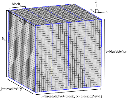
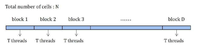
Figure 2: Connection between threads and structured cells.

Figure 3: Connection between threads and unstructured cells.

The CUDA threads are organized into thread blocks, and thread blocks constitute a thread grid. The thread grid may be seen as a computational structure on GPUs, which can be corresponded to computational cells. In the previous study GKS-GPU , the three-dimensional structured meshes are used, and a simple partition of mesh is given in Figure.3. Assume that the total number of meshes is $N_{x}\times N_{y}\times N_{z}$, and the three-dimensional computational domain is divided into $\text{block}_{x}$ parts in $x$-direction, where $\text{block}_{x}$ is an integer defined according to tests. The variables ”dimGrid” and ”dimBlock” are defined to set a two-dimensional grid, which consist of two-dimensional blocks as follows

$${\rm dimGrid} ={\rm dim3}(N_{z},N_{x}/\text{block}_{x},1),$$

$${\rm dimBlock} ={\rm dim3}(\text{block}_{x},N_{y},1).$$

It is natural to assign one thread to complete computations of a cell $K_{ijk}$, and the one-to-one correspondence of thread block index and cell index $(i,j,k)$ is simpliy given as follows

$$i =\text{threadidx}\%\text{x}+\text{block}_{x}*(\text{blockidx}\%\text{y}-1),$$

$$j =\text{threadidx}\%\text{y},$$

$$k =\text{blockidx}\%\text{x}.$$

For the unstructured meshes, the data for cells, interfaces and nodes are stored one-dimensionally. Compared with the structured meshes, the partition for blocks becomes simpler. As shown in in Figure.3, the cells can be divided into $D$ blocks, where $N$ is the total number of cells. For each block, it contains some threads and the maximum number of threads in block is 1024. It is supposed that each block contains $T$ threads and $N=D\times T$ for example. If $N$ is not divisible by $T$, an extra block is needed. The variables ”dimGrid” and ”dimBlock” are defined as

$${\rm dimGrid} ={\rm dim3}(\text{D},1,1),$$

$${\rm dimBlock} ={\rm dim3}(\text{T},1,1).$$

Thus, the one-to-one correspondence for cell and thread ID for parallel computation is given by

$$i=\text{threadidx}\%\text{x}+\text{T}*(\text{blockidx}\%\text{x}-1).$$

Main parts of the HGKS code are labeled blue in Algorithm.1, and the way to implement these parts in parallel on GPU is using kernels. The kernel is a subroutine, which executes at the same time by many threads on GPU, and the kernel for WENO reconstruction is given as an example to show the main idea of CUDA program. The Nvidia GPU is consisted of multiple streaming multiprocessors (SMs). Each block of grid is distributed to one SM, and the threads of block are executed in parallel on SM. The executions are implemented automatically by GPU. Thus, the GPU code can be implemented with specifying kernels and grids.

   Initial condition

  while TIME $\leq$ TSTOP do

     STEP 1 : Calculation of time step

     STEP 2 : WENO reconstruction

     $\text{block}_{N}$ $=$ ${\rm N}/T$  % ${\rm N}$ is the number of cell interfaces

     dimGrid $=$ dim3($\text{block}_{N}$,1,1)

     dimBlock $=$ dim3(T,1,1)

     CALL WENO$<<<$dimGrid,dimBlock$>>>$  % kernel for reconstruction and flux calculation

     istat=cudaDeviceSynchronize()  % blocking the current device until all preceeding tasks have completed

     STEP 3 : Update of flow variables (Jacobi iteration or two-stage method)

  end while Output of flow field

Algorithm 1 Program for unstructured HGKS

5 Numerical tests

In this section, numerical tests for both inviscid and viscous flows will be presented to validate the current scheme. For the inviscid flows, the collision time $\tau$ takes

$$\tau=\epsilon\Delta t+C\displaystyle|\frac{p_{l}-p_{r}}{p_{l}+p_{r}}|\Delta t,$$

where $\epsilon=0.01$ and $C=1$. For the viscous flows, we have

$$\tau=\frac{\mu}{p}+C\displaystyle|\frac{p_{l}-p_{r}}{p_{l}+p_{r}}|\Delta t,$$

where $p_{l}$ and $p_{r}$ denote the pressure on the left and right sides of the cell interface, $\mu$ is the dynamic viscous coefficient and $p$ is the pressure at the cell interface. In smooth flow regions, it will reduce to

$$\tau=\frac{\mu}{p}$$

In the computation, the poly gas is used and the specific heat ratio takes $\gamma=1.4$. For the numerical examples, the two-stage method is used for the unsteady problems, and the LU-SGS method is used for the steady problems.

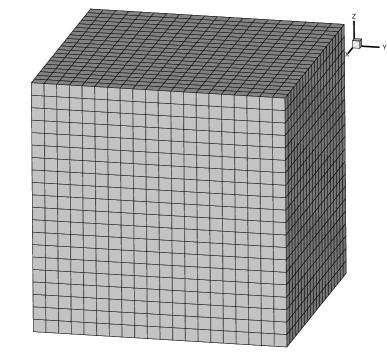
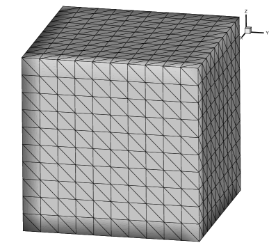
Figure 4: Accuracy test: the three-dimensional hexahedron mesh with $20^{3}$ cells (left) and tetrahedron mesh $10^{3}\times 6$ cells (right) for accuracy test.

  mesh $L^{1}$ error Order $L^{2}$ error Order $10^{3}$ 5.2689E-01 2.0675E-01 $20^{3}$ 1.0636E-01 2.3085 4.1798E-02 2.3064 $40^{3}$ 1.4729E-02 2.8521 5.7712E-03 2.8565 $80^{3}$ 1.8840E-03 2.9668 7.3678E-04 2.9695  

Table 1: Accuracy test: errors and orders of accuracy with uniform hexahedron meshes.

  mesh $L^{1}$ error Order $L^{2}$ error Order $5^{3}\times 6$ 3.7642E-01 1.4740E-01 $10^{3}\times 6$ 6.0508E-02 2.6371 2.4031E-02 2.6167 $20^{3}\times 6$ 7.8292E-03 2.9502 3.1387E-03 2.9366 $40^{3}\times 6$ 9.9153E-04 2.9811 4.0739E-04 2.9456  

Table 2: Accuracy tests: errors and orders of accuracy with tetrahedron meshes.

5.1 Accuracy test

In this case, the three-dimensional advection of density perturbation is used to test the order of accuracy with the hexahedron and tetrahedron meshes. For this case, the computational domain is $[0,2]\times[0,2]\times[0,2]$ and the initial condition is given as follows

$$\rho_{0} (x,y,z)=1+0.2\sin(\pi(x+y+z)),~{}p_{0}(x,y,z)=1,$$

$$U_{0}(x,y,z)=1,~{}V_{0}(x,y,z)=1,~{}W_{0}(x,y,z)=1.$$

The periodic boundary condition is applied on all boundaries, and the exact solution is

$$\rho(x,y ,z,t)=1+0.2\sin(\pi(x+y+z-t)),~{}p(x,y,z,t)=1,$$

$$U(x,y,z,t)=1,~{}V(x,y,z,t)=1,~{}W(x,y,z,t)=1.$$

In smooth flow regions, $\tau=0$ and the gas-distribution function reduces to

$$f(\bm{x}_{m_{1},m_{2}},t,\bm{u},\varsigma)=g(1+At).$$

For the hexahedron meshes, the uniform meshes with $\Delta x=\Delta y=\Delta z=2/N$ are used. The $L^{1}$ and $L^{2}$ errors and orders of accuracy at $t=2$ are presented in Tab.2, where the expected order of accuracy is achieved. For the tetrahedron meshes, a series of meshes with $6\times N^{3}$ cells are used, where every cubic is divided into six tetrahedron cells. The $L^{1}$ and $L^{2}$ errors and orders of accuracy at $t=2$ are presented in Tab.2, where the expected third-order of accuracy is also achieved. The mesh and the density distributions for the hexahedron mesh with $N=32$, and for the tetrahedron mesh with $N=20$ are given in Fig.4.

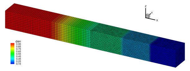
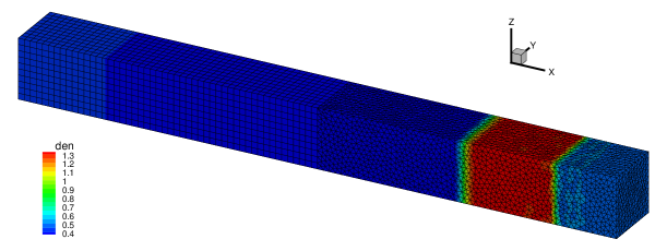
Figure 5: Riemann problem: the three-dimensional mesh and density distributions for Sod problem (left) at $t=0.2$ and Lax problem (right) at $t=0.16$ for the hybrid mesh.

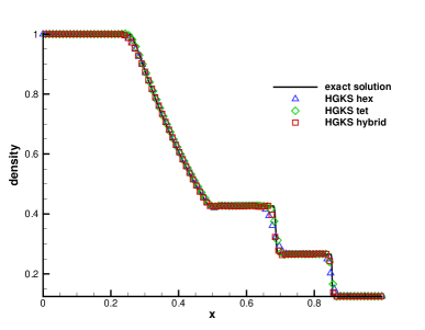
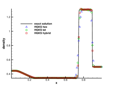
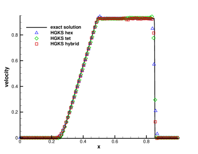
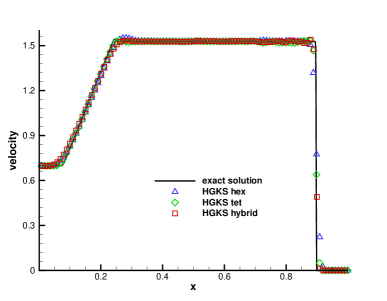
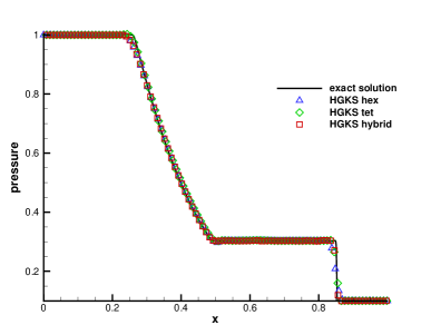
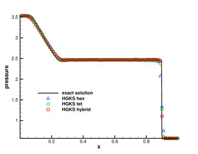
Figure 6: Riemann problem: density, velocity and pressure distributions for Sod problem (left) at $t=0.2$ and Lax problem (right) at $t=0.16$ at the center horizontal line of hexahedral, tetrahedral and hybrid meshes.

5.2 Riemann problems

In this case, two one-dimensional Riemann problems are tested by the third-order WENO scheme on the hybrid meshes which consist of tetrahedral, pyramidal and hexahedral cells. The first one is the Sod problem, and the initial condition is given as follows

$$(\rho,U,V,W,p)=\begin{cases}(1,0,0,0,1),0\leq x<0.5,\\ (0.125,0,0,0,0.1),0.5\leq x\leq 1.\end{cases}$$

The second one is the Lax problem, and the initial condition is given as follows

$$(\rho,U,V,W,p)=\begin{cases}(0.445,0.698,0,0,3.528),0\leq x<0.5,\\ (0.5,0,0,0,0.571),0.5\leq x\leq 1.\end{cases}$$

For these two cases, the computational domain is $[0,1]\times[0,0.1]\times[0.1]$. This case is tested by hybrid mesh with total 44451 cells, including 5000 hexahedron cells, 100 prism cells and 39351 tetrahedron cells. The mesh size is $h=1/100$. As comparison, these two cases are also tested with hexahedral and tetrahedral meshes. The uniform mesh with $100\times 10\times 10$ cells for the hexahedral mesh and 59003 cells with mesh size $h=1/100$ for the tetrahedral mesh are used. Non-reflection boundary condition is adopted at the left and right boundaries of the computational domain, and reflection boundary condition is adopted at other boundaries of the computational domain. The three-dimensional mesh and density distributions for Sod problem at $t=0.2$ and Lax problem at $t=0.16$ are given in Fig.5 for hybrid mesh. The numerical results of density, velocity and pressure for the Sod problem at $t=0.2$ and for the Lax problem at $t=0.16$ are presented in Fig.6 with $x\in[0,1],y=z=0$ for hexahedral, tetrahedral and hybrid meshes. The exact solutions are also given. The numerical results agree well with the exact solution, and the discontinuities are well resolved by the current scheme. As expected, the tetrahedral mesh contains more cells and resolves the discontinuities better than the hexahedral mesh.

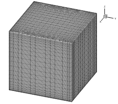
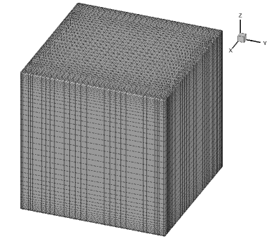
Figure 7: Lid-driven cavity flow: the local computational mesh and pressure distribution.

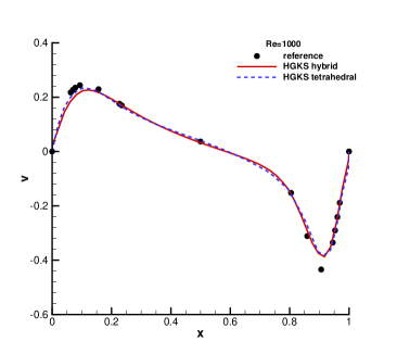
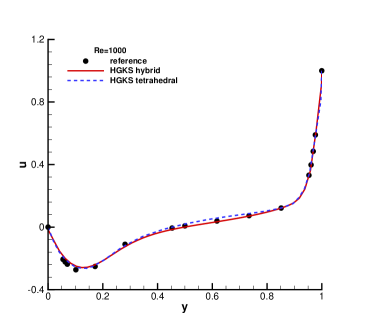
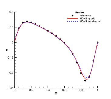
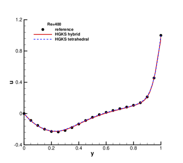
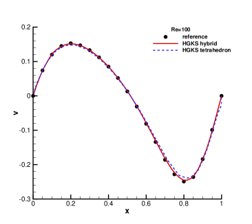
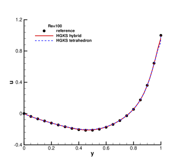
Figure 8: Lid-driven cavity flow: the steady state U-velocity profiles along the vertical centerline, V-velocity profiles along the horizontal centerline for $Re=1000,400$ and $100$.

5.3 Lid-driven cavity flow

The lid-driven cavity problem is one of the most important benchmarks for numerical Navier-Stokes solvers. The fluid is bounded by a unit cubic $[0,1]\times[0,1]\times[0,1]$ and driven by a uniform translation of the top boundary with $y=1$. In this case, the flow is simulated with Mach number $Ma=0.15$ and all the boundaries are isothermal and nonslip. Numerical simulations are conducted with the Reynolds numbers of $Re=1000$, $400$ and $100$. This case is performed by both hybrid and tetrahedral meshes. The tetrahedral mesh contains $6\times 20^{3}$ cells, in which every cuboid is divided into six tetrahedron cells. The hybrid mesh contains $1.6\times 40^{3}$ cells, including $76800$ prisms and $25600$ hexahedrons. To improve the resolution, the mesh near the well is refined and both meshes are shown in Fig.7. The three cases correspond to the convergent solutions, and the LU-SGS method is used for the temporal discretization. The $U$-velocity profiles along the vertical centerline line, $V$-velocity profiles along the horizontal centerline in the symmetry $x-y$ plane and the benchmark data for $Re=1000$ Case-Albensoeder , $Re=400$ and $Re=100$ Case-Shu are shown in Fig.8. The numerical results agree well with the benchmark data. For this case, a coarse mesh is used, especially for the tetrahedral meshes. The agreement between them shows that current HGKS is capable of simulating three-dimensional laminar flows.

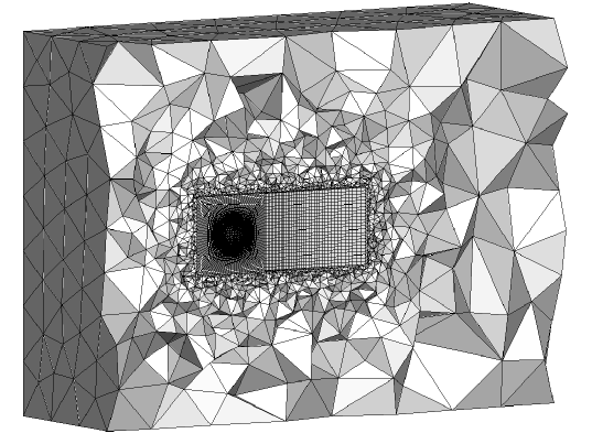
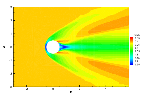
Figure 9: Flows passing through a sphere: the mesh distribution.

Figure 10: Flows passing through a sphere: the Mach number distribution at vertical centerline planes with $Ma_{\infty}=3.2$ for the inviscid flow.

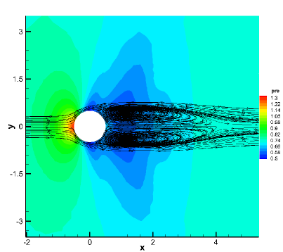
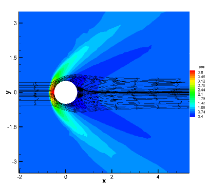
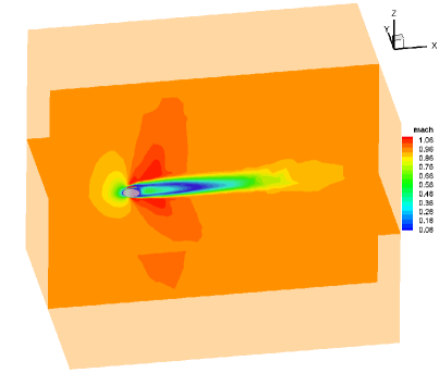
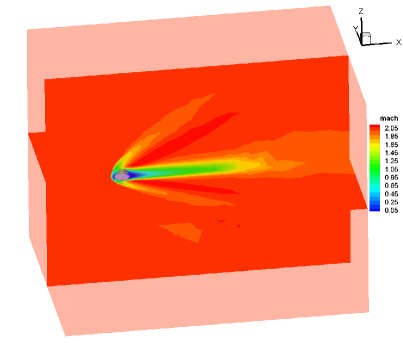
Figure 11: Flows passing through a sphere: the pressure and streamline distributions at vertical centerline planes with $Ma_{\infty}=0.95$ and $2.0$.

Figure 12: Flows passing through a sphere: the Mach number distributions at vertical centerline planes with $Ma_{\infty}=0.95$ and $2.0$.

  scheme $\phi$ $L$ WENO6 Case-Nagata 111.5 3.48 HGKS-compact scheme GKS-high-2 112.7 3.30 Current scheme 107.0 3.49  

Table 3: Flows passing a sphere: quantitative comparisons of separation angle $\phi$ and closed wake length $L$ for $Ma_{\infty}=0.95$ and $Re=300$.

  scheme $\phi$ $L$ Shock stand-off WENO6 Case-Nagata 150.9 0.38 0.21 HGKS-compact scheme GKS-high-2 148.5 0.45 0.28-0.31 Current scheme 149.8 0.34 0.22  

Table 4: Flows passing a sphere: quantitative comparisons of separation angle $\phi$, closed wake length $L$ and shock stand-off for $Ma_{\infty}=2$ and $Re=300$.

5.4 Flows passing a sphere

This case is used to test the capability in resolving the low-speed to hypersonic flows, and the initial condition is given as a free stream condition

$$(\rho,U,V,W,p)_{\infty}=(1,Ma_{\infty},0,0,1/\gamma),$$

where $\gamma=1.4$. The computation domain is $[-5,15]\times[-7.5,7.5]\times[-7.5,7.5]$. As shown in Fig.10, the hybrid mesh with $462673$ cells is used. The inlet and outlet boundary conditions are given according to Riemann invariants, the slip adiabatic boundary condition is used for inviscid flows and the non-slip adiabatic boundary condition is imposed for viscous flows on the surface of sphere.

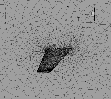
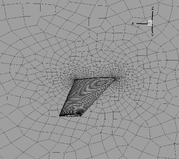
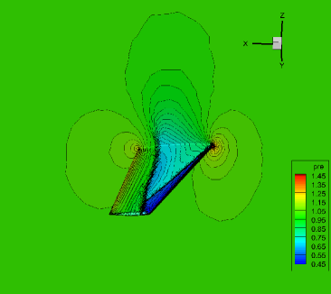
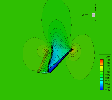
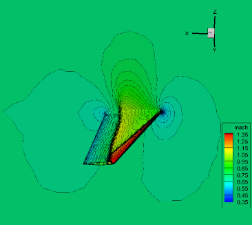
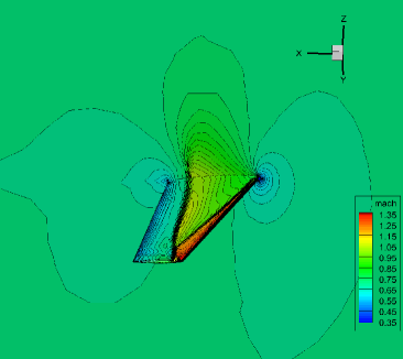
Figure 13: ONERA M6 wing: the local mesh, pressure and Mach number distribution for the inviscid flow with tetrahedral and hybrid meshes.

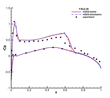
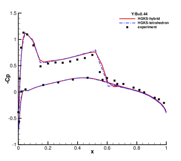
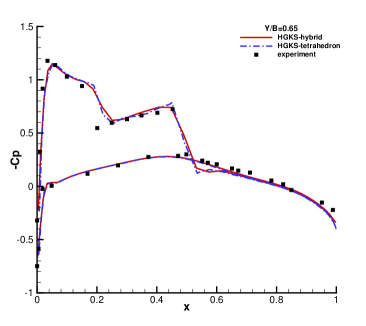
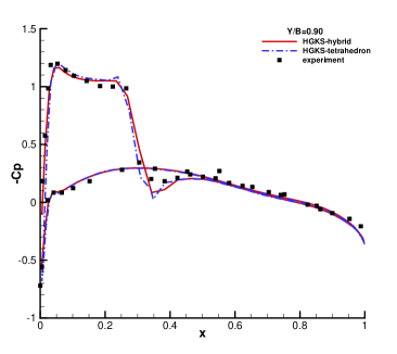
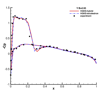
Figure 14: ONERA M6 wing: the pressure coefficient distributions at $Y/B=0.20$, $0.44$, $0.65$, $0.80$, $0.90$ and $0.95$ for the inviscid flow with tetrahedral and hybrid meshes.

For the hyperbolic inviscid flows, this case is tested with the explicit and implicit schemes. For the explicit scheme, the Mach number of inflow can be tested only up to $Ma_{\infty}=2.2$, and the codes blow up due to the vacuum state forms at the leeward side of the sphere. The implicit scheme is more robust than the explicit scheme, and the Mach number of inflow can be tested up to $Ma_{\infty}=3.2$. The Mach number distribution at vertical centerline planes is given in Fig.10, where the largest Mach number is 3.97 and no special treatment is needed for reconstruction. For the viscous flows, two cases with $Re=300$ are tested with unstructured hybrid mesh, including supersonic flow with $Ma_{\infty}=2.0$ and transsonic flow with $Ma_{\infty}=0.95$. For these two cases, the computation will converge to steady states, and the LU-SGS method is used for the temporal discretization. For the hypersonic flow, the dynamic viscosity is given by

$$\mu=\mu_{\infty}(\frac{T}{T_{\infty}})^{0.7},$$

where $T_{\infty}$ and $\mu_{\infty}$ are free stream temperature and viscosity. The pressure, Mach number and streamline distributions are presented in Fig.12 and Fig.12 for the two cases, and the robustness of the current scheme is validated. The quantitative results of separation angle $\phi$ and closed wake length $L$ are given in Table.4 and Table.4. For the supersonic case, the position of shock stand-off is also given in Table.4. Quantitative results agree well with the benchmark solutions Case-Nagata , and the slight deviation of compact gas-kinetic scheme GKS-high-2 might caused by the coarser mesh.

5.5 Transonic flow around ONERA M6 wing

The transonic flow around the ONERA M6 wing is a standard benchmark for engineering simulations. Besides the three-dimensional geometry, the flow structures are complex including the interaction of shock and turbulent boundary. Thus, it is a good candidate to test the performance of the extended BGK model and high-order gas-kinetic scheme. The inviscid flow around the wing is first tested, which corresponds to a rough prediction of the flow field under a very high Reynolds number. The incoming Mach number and angle of attack are given by

$$Ma_{\infty}=0.8395,~{}AoA=3.06^{\circ}.$$

This case is performed by both hybrid and tetrahedral meshes, which are given in Fig.13. The tetrahedral includes 294216 cells and the hybrid mesh includes 201663 cells. The subsonic inflow and outflow boundaries are all set according to the local Riemann invariants, and the adiabatic and slip wall condition is imposed on the solid wall. The local pressure and Mach number distributions are also shown in Fig.13, and the $\lambda$ shock is well resolved by the current schemes. The comparisons on the pressure distributions at the semi-span locations $Y/B=0.20$, $0.44$, $0.65$, $0.80$, $0.90$ and $0.95$ of the wing are given in Fig.14. The numerical results quantitatively agree well with the experimental data Case-Schmitt .

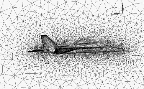
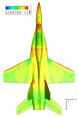
Figure 15: Flow over a $YF-17$ fighter: the local mesh distribution.

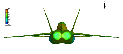
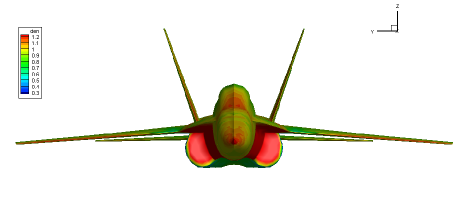
a b c d

Figure 16: Flow over a $YF-17$ fighter: the steady state density distributions from the top (a), bottom (b), forward (c) and backward (d) views.

5.6 Flow over a $YF-17$ fighter

The inviscid supersonic flow passing through a complete aircraft model is computed. The computational mesh for a YF-17 Cobra fighter model is shown in Fig.16, which is provided at ”https:// cgns.github. io/CGNSFiles. html”. The mesh includes 174127 tetrahedral cells. The incoming Mach number and angle of attack are given by

$$Ma_{\infty}=1.05,~{}AoA=0^{\circ}.$$

The surface density distributions from the top, bottom, forward and backward views are given in Fig.16. Complicated shocks appear in the locations including the nose, cockpit-canopy wing, horizontal stabilizer, and vertical stabilizer. This cases validate the capability of current scheme to handle complicated geometry, such as the mesh skewness near the wing tips and the lack of neighboring cell for the cell near boundary corners.

  Case cell face Jacobi+CPU LUSGS+CPU Cavity 102400 274560 568 s 703 s Sphere 462673 1174016 6590 s 8210 s  

Table 5: Efficiency comparison: the computational time per 1000 steps for Jacobian and LUSGS iterations with CPU code.

  Case Jacobi+GPU Jacobi+CPU Speedup Cavity 97 s 568 s 5.86 Sphere 1093 s 6590 s 6.03  

Table 6: Efficiency comparison: the computational time per 1000 steps and speedup for GPU and CPU code with Jacobian iteration.

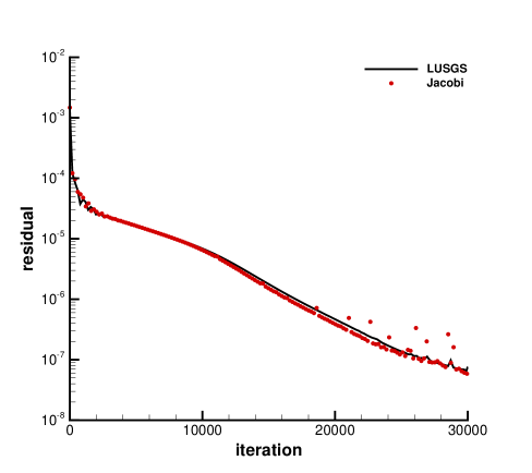
Figure 17: Efficiency comparison: the comparison of convergence history with Jacobian and LUSGS iterations for the cavity case.

5.7 Efficiency comparison of CPU and GPU

The efficiency comparison of CPU and GPU codes is provided with the current scheme. The CPU code is run with Intel i7-11700 CPU using Intel Fortran compiler with OpenMP directives, while Nvidia TITAN RTX is used for GPU code with Nvidia CUDA and NVFORTRAN compiler. The clock rates of GPU and CPU are 1.77 GHz and 2.50 GHz respectively, and the double precision is used in computation. The lid-driven cavity flow with $Re=1000$ and the hyperbolic inviscid flow passing a sphere with $Ma_{\infty}=2$ on three dimensional hybrid unstructured meshes are used to test the efficiency. The HGKS with Jacobi iteration is implemented with GPU and CPU with $k_{\max}=3$. The HGKS with LUSGS iteration is only implemented with CPU. In the computation, the update part is implemented sequentially and the left parts are implemented in parallel. For these two cases, the computational time of Jacobi and LUSGS implicit iterations with CPU code are given in Table.6. Due to the smooth GKS flux Eq.(12) used in cavity case and the full GKS flux Eq.(11) used in sphere case, and more control volumes, the sphere case costs more computational times. Meanwhile, because of the sequential update part, the LUSGS method costs more computational times. The computational times of GPU code and speedups for the two cases are given in Table.6, where speedup is defined as

$$\text{speedup}=\frac{\text{computational time of CPU}}{\text{computational time of GPU}}.$$

As shown in Table.6, 5x-6x speedup is achieved for Jacobian GPU code compared with Jacobi CPU code. As expected, the acceleration effect is more obvious as the number of cells increases. The comparison of the convergence histories of LUSGS and Jacobi implicit iterations for the cavity case is given in Fig.17. For both the Jacobian and LUSGS iterations, it can be observed that the residuals converge to the order of $10^{-8}$. However, the convergence rate of Jacobian iteration is not as stable as that of LUSGS iteration. In the future, the more efficient parallel implicit algorithm will be considered, and more challenging problems for compressible flows will be investigated.

6 Conclusion

In the paper, a third-order gas-kinetic scheme is developed on three-dimensional arbitrary unstructured meshes for compressible inviscid and viscous flows. In the classical WENO schemes, the high-order of accuracy is obtained by the non-linear combination of lower order polynomials from the candidate stencils. To achieve the spatial accuracy, a weighted essentially non-oscillatory (WENO) reconstruction is developed on the three-dimensional arbitrary unstructured meshes. However, Due to the topology complicated of the arbitrary unstructured meshes with tetrahedral, pyramidal, prismatic and hexahedral cells, great difficulties are introduced for the classical WENO schemes. A simple strategy of selecting stencils for reconstruction is adopted and the topology independent linear weights are used for tetrahedron, pyramid, prism and hexahedron. Incorporate with the two-stage fourth-order temporal discretization, the explicit high-order gas-kinetic schemes are developed for unsteady problems. With lower-upper symmetric Gauss-Seidel (LU-SGS) method, the implicit high-order gas-kinetic schemes are developed for steady problems. Various three-dimensional numerical experiments, including the inviscid flows and laminar flows, are presented. The results validate the accuracy and robustness of the proposed scheme. In the future, the high-order gas-kinetic scheme on arbitrary unstructured meshes will be applied for the engineering turbulent flows with high-Reynolds numbers.

References

- (1) R. Abgrall, On essentially non-oscillatory schemes on unstructured meshes: analysis and implementation, J. Comput. Phys. 114 (1994) 45-58.
- (2) S. Albensoeder, H.C. Kuhlmann, Accurate three-dimensional lid-driven cavity flow, J. Comput. Phys. 206 (2005) 536-558.
- (3) D.S. Balsara, S. Garain, C.-W. Shu. An efficient class of WENO schemes with adaptive order, J. Comput. Phys. 326 (2016) 780-804.
- (4) D.S. Balsara, S. Garain, V. Florinski, W. Boscheri, An efficient class of WENO schemes with adaptive order for unstructured meshes, J. Comput. Phys. 404 (2020) 109062.
- (5) P.L. Bhatnagar, E.P. Gross, M. Krook, A Model for Collision Processes in Gases I: Small Amplitude Processes in Charged and Neutral One-Component Systems, Phys. Rev. 94 (1954) 511-525.
- (6) R. Borges, M. Carmona, B. Costa, W. S. Don, An improved weighted essentially non-oscillatory scheme for hyperbolic conservation laws, J. Comput. Phys. 227 (2008) 3191-3211.
- (7) G.Y. Cao, L. Pan, K. Xu, High-order gas-kinetic scheme with parallel computation for direct numerical simulation of turbulent flows, J. Comput. Phys. 448 (2022) 110739.
- (8) G.Y. Cao, H.M. Su, J.X Xu, K. Xu, Implicit high-order gas kinetic scheme for turbulence simulation, Aerospace Science and Technology 92 (2019) 958-971.
- (9) S. Chapman, T.G. Cowling, The Mathematical theory of non-uniform gases, third edition, Cambridge University Press, (1990).
- (10) J. Cheng, X.Q. Yang, X.D Liu, T.D. Liu, H. Luo, A direct discontinuous Galerkin method for the compressible Navier-Stokes equations on arbitrary grids, J. Comput. Phys. 327 (2016) 484-502.
- (11) B. Cockburn, C.-W. Shu, The Runge-Kutta discontinuous Galerkin method for conservation laws V: multidimensional systems, Journal of Computational Physics 141 (1998) 199-224.
- (12) Z.F. Du, J.Q. Li, A Hermite WENO reconstruction for fourth order temporal accurate schemes based on the GRP solver for hyperbolic conservation laws, J. Comput. Phys. 355 (2018) 385-396.
- (13) M. Dumbser, D. Balsara, E. Toro, C.D. Munz, A unified framework for the construction of one-step finite volume and discontinuous Galerkin schemes on unstructured meshes, J. Comput. Phys. 227 (2008) 8209-8253.
- (14) M. Dumbser, M. Käser, Arbitrary high order non-oscillatory finite volume schemes on unstructured meshes for linear hyperbolic systems, J. Comput. Phys. 221 (2007) 693-723.
- (15) C. Hu, C. W. Shu, Weighted essentially non-oscillatory schemes on triangular meshes, J. Comput. Phys. 150 (1999) 97-127.
- (16) A. Jameson, S. Yoon, Lower-upper implicit schemes with multiple grids for the Euler equations, AIAA J. 25 (7) (1987) 929-935.
- (17) X. Ji, F. Zhao, W. Shyy, K. Xu, A HWENO reconstruction based high-order compact gas-kinetic scheme on unstructured mesh, J. Comput. Phys. 410 (2020) 109367.
- (18) G.S. Jiang, C.-W. Shu, Efficient implementation of weighted ENO schemes, J. Comput. Phys. 126 (1996) 202-228.
- (19) J. Jiang, Y.H. Qian, Implicit gas-kinetic BGK scheme with multigrid for 3d stationary transonic high-Reynolds number flows, Comput. Fluids 66 (2012) 21-28.
- (20) O. Kolb, On the full and global accuracy of a compact third order WENO scheme, SIAM J. Numer. Anal. 52 (2014) 2335-2355.
- (21) D. Levy, G. Puppo, G. Russo, Central WENO schemes for hyperbolic systems of conservation laws, Math. Model. Numer. Anal. 33 (1999) 547-571.
- (22) D. Levy, G. Puppo, G. Russo, Compact central WENO schemes for multidimensional conservation laws, SIAM J. Sci. Comput. 22 (2000) 656-672.
- (23) J.Q. Li, Z.F. Du, A two-stage fourth order time-accurate discretization for Lax-Wendroff type flow solvers I. hyperbolic conservation laws, SIAM J. Sci. Computing, 38 (2016) 3046-3069.
- (24) X.D. Liu, S. Osher, T. Chan, Weighted essentially non-oscillatory schemes, J. Comput. Phys. 115 (1994) 200-212.
- (25) T. Nagata, T. Nonomura, S. Takahashi, Y. Mizuno, K. Fukuda. Investigation on subsonic to supersonic flow around a sphere at low Reynolds number of between 50 and 300 by direct numerical simulation. Physics of Fluids, 28 (2016) 056101.
- (26) L. Pan, K. Xu, Q.B. Li, J.Q. Li, An efficient and accurate two-stage fourth-order gas-kinetic scheme for the Navier-Stokes equations, J. Comput. Phys. 326 (2016) 197-221.
- (27) L. Pan, J. Li, K. Xu, A few benchmark test cases for higher-order Euler solvers, Numer. Math., Theory Methods Appl. 10 (4) (2017) 711-736.
- (28) L. Pan, G.Y. Cao, K. Xu, Fourth-order gas-kinetic scheme for turbulence simulation with multi-dimensional WENO reconstruction, Computers and Fluids 221 (2021) 104927.
- (29) J.X. Qiu, C.-W. Shu, Hermite WENO schemes and their application as limiters for Runge-Kutta discontinuous Galerkin method, III: unstructured meshes, J. Sci. Comput. 39 (2009) 293-321.
- (30) V. Schmitt, F. Charpin, Pressure distributions on the ONERA-M6-wing at transonic Mach numbers, Experimental Data Base for Computer Program Assessment, Report of the Fluid Dynamics Panel Working Group 04, AGARD AR 138, 1979.
- (31) J. Shi, C. Hu, C.W. Shu, A Technique of Treating Negative Weights in WENO Schemes, J. Comput. Phys. 175 (2002) 108-127.
- (32) C. Shu, L. Wang, Y. T. Chew, Numerical Computation of Three-dimensional Incompressible Navier.Stokes Equations in Primitive Variable form by DQ Method, International Journal for Numerical Methods in Fluids 43 (2003) 345-368.
- (33) S. Tan, Q.B. Li. Time-implicit gas-kinetic scheme. Computers Fluids, 144 (2017) 44-59.
- (34) V. Titarev, P. Tsoutsanis, D. Drikakis, WENO schemes for mixed-element unstructured meshes, Commun. Comput. Phys. 8 (2010) 585-609.
- (35) P. Tsoutsanis, V. Titarev, D. Drikakis, WENO schemes on arbitrary mixed-element unstructured meshes in three space dimensions, J. Comput. Phys. 230 (2011) 1585-1601.
- (36) P. Tsoutsanis, A.F. Antoniadis, D. Drikakis, WENO schemes on arbitrary unstructured meshes for laminar, transitional and turbulent flows, J. Comput. Phys. 256 (2014) 254-276.
- (37) Z.J. Wang, Spectral (finite) volume method for conservation laws on unstructured grids: basic formulation, J. Comput. Phys. 178 (2002) 210-251.
- (38) Z.J. Wang, H. Gao, A unifying lifting collocation penalty formulation including the discontinuous Galerkin, spectral volume/difference methods for conservation laws on mixed grids. J. Comput. Phys. 228 (2009) 8161-8186.
- (39) Y.H. Wang, L. Pan, Three-dimensional discontinuous Galerkin based high-order gas-kinetic scheme and GPU implementation, arXiv: 2202.13821.
- (40) K. Xu, Direct modeling for computational fluid dynamics: construction and application of unfied gas kinetic schemes, World Scientific (2015).
- (41) K. Xu, A gas-kinetic BGK scheme for the Navier-Stokes equations and its connection with artificial dissipation and Godunov method, J. Comput. Phys. 171 (2001) 289-335.
- (42) Z. Xu, Y. Liu, C.-W. Shu, Hierarchical reconstruction for discontinuous Galerkin methods on unstructured grids with a WENO-type linear reconstruction and partial neighboring cells, J. Comput. Phys. 228 (2009) 2194-2212.
- (43) Y.Q. Yang, L. Pan, K. Xu, High-order gas-kinetic scheme on three-dimensional unstructured meshes for compressible flows, Physics of Fluids 33 (2021) 096102.
- (44) S. Yoon, A. Jameson, Lower-upper symmetric-Gauss-Seidel method for the Euler and Navier-Stokes equations, AIAA J. 26 (9) (1988) 1025-1026.
- (45) F.X. Zhao, L. Pan, S.H. Wang, Weighted essentially non-oscillatory scheme on unstructured quadrilateral and triangular meshes for hyperbolic conservation laws, J. Comput. Phys. 374 (2018) 605-624.
- (46) F.X. Zhao, X. Ji , W. Shyy, K. Xu, A compact high-order gas-kinetic scheme on unstructured mesh for acoustic and shock wave computations, J. Comput. Phys. 449 (2022) 110812
- (47) J. Zhu, J.X. Qiu, A new fifth order finite difference weno scheme for solving hyperbolic conservation laws. J. Comput. Phys. 318 (2016) 110-121.
- (48) J. Zhu, J.X. Qiu, New finite volume weighted essentially non-oscillatory scheme on triangular meshes, SIAM J. Sci. Computing, 40 (2018) 903-928.
- (49) Y.J. Zhu, C.W. Zhong, K. Xu.Implicit unified gas-kinetic scheme for steady state solutions in all flow regimes. Journal of Computational Physics, 315 (2016) 16-38.