Further Evidence of Modified Spin-down in Sun-like Stars:
Pileups in the Temperature–Period Distribution

Abstract

We combine stellar surface rotation periods determined from NASA’s Kepler mission with spectroscopic temperatures to demonstrate the existence of pileups at the long-period and short-period edges of the temperature–period distribution for main-sequence stars with temperatures exceeding $\sim$5500 K. The long-period pileup is well-described by a curve of constant Rossby number, with a critical value of $\mathrm{Ro_{crit}}~{}\lesssim~{}\mathrm{Ro_{\odot}}$. The long-period pileup was predicted by van Saders et al. (2019) as a consequence of weakened magnetic braking, in which wind-driven angular momentum losses cease once stars reach a critical Rossby number. Stars in the long-period pileup are found to have a wide range of ages ($\sim$2–6 Gyr), meaning that, along the pileup, rotation period is strongly predictive of a star’s surface temperature but weakly predictive of its age. The short-period pileup, which is also well-described by a curve of constant Rossby number, is not a prediction of the weakened magnetic braking hypothesis but may instead be related to a phase of slowed surface spin-down due to core–envelope coupling. The same mechanism was proposed by Curtis et al. (2020) to explain the overlapping rotation sequences of low-mass members of differently aged open clusters. The relative dearth of stars with intermediate rotation periods between the short- and long-period pileups is also well-described by a curve of constant Rossby number, which aligns with the period gap initially discovered by McQuillan et al. (2013a) in M-type stars. These observations provide further support for the hypothesis that the period gap is due to stellar astrophysics, rather than a non-uniform star-formation history in the Kepler field.

1 Introduction

Solar-type and low-mass stars ($M\lesssim 1.3$ $M_{\odot}$) lose mass and angular momentum through magnetized winds (Parker, 1958; Weber & Davis, 1967; Mestel, 1968; Kawaler, 1988). Consequently, stellar rotation rates are observed to decline with age. Skumanich (1972) presented the first attempt to calibrate this age-rotation relationship using the rotation periods of Sun-like stars in open clusters with independently determined ages, finding a $P_{\mathrm{rot}}\propto t^{1/2}$ scaling, where $t$ is stellar age. In the intervening decades, observational determinations of stellar rotation periods among open cluster members revealed how stellar spin rates evolve in more detail, leading to the calibration of the so-called gyrochronology method (Barnes, 2003, 2007, 2010; Mamajek & Hillenbrand, 2008; Meibom et al., 2009; Angus et al., 2019).

The arrival of continuous, high-precision, long-baseline photometry from NASA’s Kepler space telescope (Borucki et al., 2010) provided a watershed moment for stellar rotation studies, yielding period detections for tens of thousands of stars (e.g. Reinhold et al., 2013; McQuillan et al., 2014; Santos et al., 2021) and allowing for gyrochronology to be extended to older ages (e.g. Meibom et al., 2011, 2015). NASA’s subsequent K2 (Howell et al., 2014) and TESS (Ricker et al., 2015) missions propelled the field of stellar rotation further still, providing an exquisitely detailed picture of how spin rates evolve for stars with a broad range of masses and ages in stellar associations (e.g. Douglas et al., 2016, 2017, 2019; Rebull et al., 2016, 2017, 2018, 2020; Curtis et al., 2019a, b, 2020). New and evermore precise data is becoming available at a rate that is outpacing efforts to re-calibrate gyrochronology, which is necessary to capture the complex relationship between a star’s spin and its age.

For example, efforts to calibrate gyrochronology relations using Kepler asteroseismic targets revealed tension with relations calibrated to open clusters and found that rotation periods could not be described by a single power-law relation with age (Angus et al., 2015). This tension, at least in part, is due to the fact that standard gyrochronology models are unable to account for the anomalously rapid rotation rates of stars older than the Sun, leading to the suggestion that stars with Rossby numbers of Ro $\gtrsim$ $\mathrm{Ro_{\odot}}$ experience a phase of weakened magnetic braking (WMB, van Saders et al., 2016).

Forward modeling simulations of the observed Kepler rotation period distribution also provided support for the WMB hypothesis over standard spin-down models, in that WMB models are better able to match the observed long-period edge (van Saders et al., 2019, hereafter vS19). Those authors also predicted a pileup of stars along the long-period edge, which they hypothesized could not be seen in the McQuillan et al. (2014) sample (hereafter MMA14) due to large errors on $T_{\mathrm{eff}}$ in the revised Kepler Input Catalog (KIC, Huber et al., 2014). While vS19 favored the WMB hypothesis to explain observations, those authors were also careful to point out that a long-period edge can be caused by detection biases, as stars with longer rotation periods (and larger Rossby numbers) have smaller amplitude variations which pose more difficulty to period-detection algorithms.

More recently, Hall et al. (2021), hereafter H21, used the asteroseismic rotation rates of Kepler dwarfs, with different selection and detection biases from the vS19 study and the present work, to argue support for the WMB model. Masuda et al. (2021), hereafter MPH21, also found support for the WMB hypothesis from inference of the rotation period distribution of Sun-like stars using stellar radii and projected rotational velocities. While the physics responsible for the weakened magnetic braking of solar-type stars is unknown, one hypothesis is that the declining efficiency of wind-driven angular momentum loss is connected to the magnetic field complexity, which may vary with Rossby number (e.g. Réville et al., 2015; van Saders et al., 2016; Garraffo et al., 2016; Metcalfe et al., 2016, 2019).

Here we examine the rotation period distribution of stars observed by Kepler, leveraging the recent release of precise spectroscopic parameters from large-scale surveys, to demonstrate the existence of pileups at the long- and short-period edges of the $T_{\mathrm{eff}}$–$P_{\mathrm{rot}}$ distribution of solar-type stars. We discuss our sample in §2, describe the steps of our analysis in §3, discuss some implications of these results in §4, and present our conclusions in §5.

2 Sample Selection

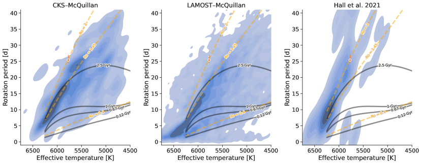
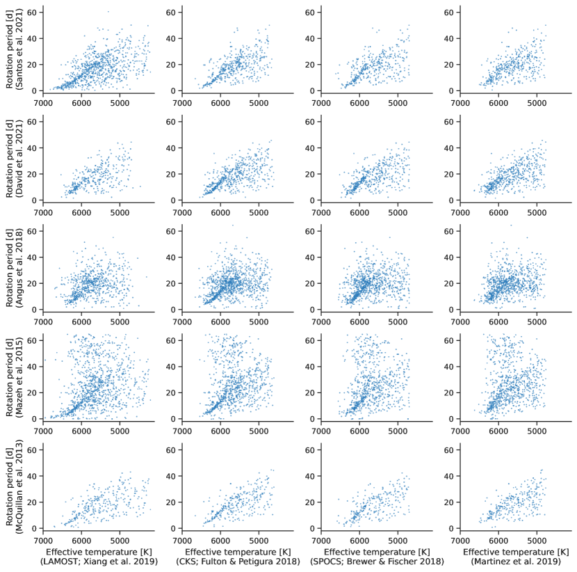
Below, we describe the samples utilized in this work. All stars characterized here were targets of NASA’s Kepler mission (Borucki et al., 2010) and have published rotation periods derived from the Kepler data. For each subsample of the Kepler field described below, we combined published rotation periods from a variety of literature sources with spectroscopic parameters provided by large-scale surveys (Figure 1).

Figure 1: The $T_{\mathrm{eff}}$-$P_{\mathrm{rot}}$ plane using rotation periods from MMA14 or, in the case of the CKS sample, McQuillan et al. (2013b) which applied an identical analysis to Kepler Objects of Interest (KOIs), with $T_{\mathrm{eff}}$ originating from the source denoted at top. The MMA14 $T_{\mathrm{eff}}$ values originate from the Kepler Input Catalog (KIC, Brown et al., 2011) or Dressing & Charbonneau (2013) for low-mass stars. The orange point in each panel indicates the Sun’s equatorial rotation period, with the errorbar capturing the range of periods measured from the activity belts. Many of the stars above the long-period pileup are subgiants which have experienced spin-down due to expansion off the main-sequence, as pointed out in vS19.

2.1 California–Kepler Survey

The CKS project acquired high-resolution spectroscopy for 1305 Kepler planet host stars (Petigura et al., 2017). CKS spectra were acquired with the Keck/HIRES spectrograph (Vogt et al., 1994) and spectroscopic parameters were determined by averaging parameters from the SpecMatch pipeline (Petigura, 2015) and SME@XSEDE, a Python implementation of the Spectroscopy Made Easy pipeline (Valenti & Piskunov, 1996). The internal (relative) errors on $T_{\mathrm{eff}}$ from the CKS catalog are estimated at $\pm$60 K, with systematic errors of $\pm$100 K estimated from comparison to other catalogs (see Table 7 of Petigura et al., 2017). The metallicity distribution of the CKS sample is centered near solar, with a mean and standard deviation of +0.03 dex and 0.18 dex, respectively.

We compiled rotation periods for these stars from a variety of literature sources including McQuillan et al. (2013b); Mazeh et al. (2015) and Angus et al. (2018). For each star in the sample we then visually inspected the Kepler light curve folded on all available literature periods, as well as the first harmonics and sub-harmonics of those periods, and recorded our preferred period along with a reliability flag. Our procedure is explained in detail in §2.1 of David et al. (2021), and rotation period vetting sheets for each Kepler Object of Interest (KOI) are publicly available through Zenodo. The vast majority of stars in the CKS sample host small planets ($R_{P}<4$ $R_{\oplus}$) and as such it is not expected that the host stars have experienced tidal spin-up from the planets.

In addition to the original CKS catalog, we also cross-matched our sample with the catalogs of Brewer & Fischer (2018) and Martinez et al. (2019), both of which presented spectroscopic parameters for CKS stars based on independent analysis of the same spectra. The Brewer & Fischer (2018) study, referred to here as SPOCS, also published elemental abundances and ages from isochrone fitting for the CKS sample. We additionally cross-matched the CKS catalog with the LAMOST DR5 catalog (Xiang et al., 2019) which is described further in §2.2. We compare the $T_{\mathrm{eff}}$–$P_{\mathrm{rot}}$ distributions of the CKS sample using $T_{\mathrm{eff}}$ and rotation periods from a variety of sources in Appendix A.

2.2 LAMOST

The LAMOST project derived homogeneous spectroscopic parameters from low-resolution ($R\sim$ 1800) LAMOST DR5 spectra for approximately 40% of the Kepler field (Zong et al., 2018; Xiang et al., 2019). A description of the LAMOST Kepler field observations is provided in De Cat et al. (2015). The Xiang et al. (2019) catalog derived stellar parameters using the DD-Payne pipeline, which builds on the method of Ting et al. (2017) by incorporating elements of the Cannon (Ness et al., 2015) and uses the overlap with GALAH DR2 and APOGEE DR14 as training data. We cross-matched the LAMOST DR5 stellar parameter catalog of Xiang et al. (2019) with the MMA14 catalog, which published rotation periods for $>$34000 Kepler targets, as well as the Santos et al. (2021) catalog (hereafter S21), which provides rotation periods for $>$55000 FGKM stars observed by Kepler.

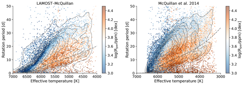
We matched 10844 LAMOST targets to 10550 unique Kepler IDs in MMA14, resulting in a sample with well-determined $P_{\mathrm{rot}}$ and spectroscopic $T_{\mathrm{eff}}$ (having a median error of 24 K). For the Kepler sources with duplicate cross-matched LAMOST sources we kept the source with a brighter Gaia DR2 $G$ magnitude. In the S21 sample we found 54982 unique cross-matched sources in LAMOST, of which 18990 have published temperatures and rotation periods. The metallicity distribution of the LAMOST–McQuillan sample is centered near solar, with a mean and standard deviation of $-0.1$ dex and 0.26 dex, respectively. There is negligible overlap (3 stars) between our LAMOST–McQuillan sample and the CKS sample since MMA14 did not publish rotation periods for KOIs, which were the targets of the CKS project. Rotation periods for KOIs are instead published in McQuillan et al. (2013b), as discussed in §2.1. Visualizations of the LAMOST–McQuillan and LAMOST–Santos samples are shown in Figure 2.

2.3 APOGEE

The Apache Point Observatory Galactic Evolution Experiment (APOGEE; Majewski et al., 2017) is a large-scale, high-resolution ($R\sim 22500$) stellar spectroscopic survey conducted at $H$-band as part of the Sloan Digital Sky Survey (SDSS-IV; Blanton et al., 2017). The spectroscopic analysis pipeline for SDSS DR16 is described in Jönsson et al. (2020). We used Gaia DR2 source IDs (Gaia Collaboration et al., 2016, 2018) to cross-match Megan Bedell’s Gaia–Kepler catalog with the APOGEE DR16 catalog (Ahumada et al., 2020). Kepler IDs were then used to cross-match this table with the MMA14 catalog. While the current overlap between Kepler targets and APOGEE is small compared to the LAMOST catalog, APOGEE DR17 will contain more dwarf stars and provide a better resource for studies such as ours. The focus of this work are overdensities in the $T_{\mathrm{eff}}$–$P_{\mathrm{rot}}$ plane, and as these appear to be less prominent when using APOGEE DR16 temperatures (Figure 1) we conclude that LAMOST and CKS provide more precise estimates of $T_{\mathrm{eff}}$ and do not analyze the APOGEE sample further.

2.4 The Sun

To place the Sun in the context of the long-period pileup, we use up-to-date estimates of the Sun’s effective temperature, color, rotation period, and age. Following the IAU 2015 Resolution B3 (Prša et al., 2016), we take the nominal effective temperature of the Sun to be $\mathcal{T}^{\mathrm{N}}_{\mathrm{eff,\odot}}=5772$ K. For the color and apparent magnitude of the Sun in the Gaia bandpasses we adopt $G_{\mathrm{BP}}-G_{\mathrm{RP}}=0.818$ mag and $G=-26.895$ mag (Casagrande & VandenBerg, 2018). For the solar rotation period we adopt the equatorial rotation period of $P_{\mathrm{eq,\odot}}~{}\approx~{}25.4$ d. While helioseismic differential rotation studies have inferred rotation periods of up to $\approx$ 36 d near the poles (Thompson et al., 2003, and references therein), sunspots are rarely observed outside the activity belts, roughly $\pm 30^{\circ}$ from the equator (Hathaway, 2015, and references therein). We therefore adopt 27 d as an approximate upper limit to the rotation period of the Sun, as it would be observed by Kepler through rotational brightness modulations. The age of the Sun is assumed to be 4.567 Gyr from Pb-Pb dating of calcium-aluminum inclusions and chondrules recovered from primitive meteorites (Bahcall et al., 1995, and references therein).

Figure 2: Two-dimensional histograms indicating the number of Kepler target stars in the $T_{\mathrm{eff}}$ –$P_{\mathrm{rot}}$ plane for the LAMOST–McQuillan sample (top row) and the LAMOST–Santos sample (bottom row). The effects of a simple cut in $\log g$ to separate subgiants and dwarfs are shown in the middle and right columns. In each panel the Sun is indicated by the orange point, with an errorbar reflecting the range of periods measured from the activity belts. The long-period pileup for dwarf stars is clearly seen to extend to the solar temperature. The short-period pileup is clearer in the smaller LAMOST–McQuillan dwarf sample, potentially because the S21 catalog detected more stars at longer periods. The secondary overdensity observed in the subgiant samples, most visible in the bottom center panel, appears to be at twice the period of the primary overdensity, potentially due to erroneously determined rotation periods.

3 Analysis

3.1 Initial observations

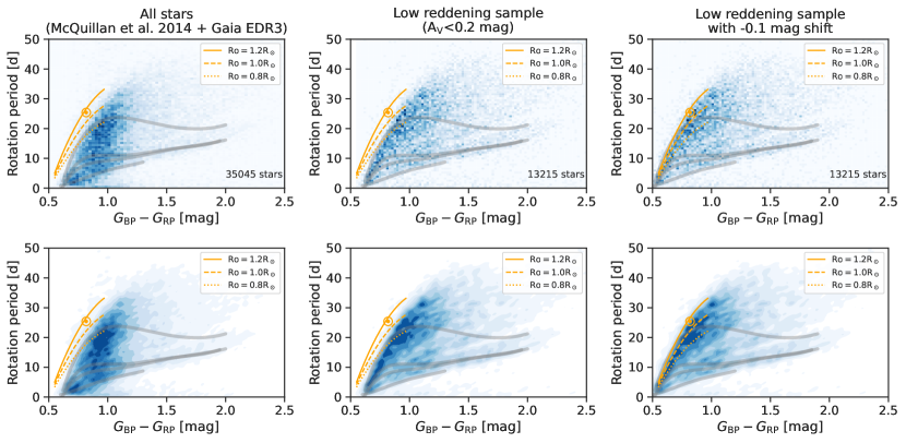
We first noted a pileup of stars along the long-period edge for stars with $T_{\mathrm{eff}}$ $>5800$ K when examining the $T_{\mathrm{eff}}$-$P_{\mathrm{rot}}$ plane for the CKS sample, using the CKS $T_{\mathrm{eff}}$ values and the vetted rotation period compilation from David et al. (2021). The pileup in that sample is visible even when sourcing $P_{\mathrm{rot}}$ uniformly from McQuillan et al. (2013b), as shown in the rightmost panel of Figure 1. Sourcing rotation periods from Mazeh et al. (2015), Angus et al. (2018), and S21 revealed that this pileup is still apparent when adopting periods uniformly from other catalogs as well (see Appendix A). It is thus the $T_{\mathrm{eff}}$ precision afforded by spectroscopic catalogs that reveal the long-period pileup. In Appendix C, we demonstrate that it is possible to recover the long-period pileup in the color–period plane using high-precision photometry from the Gaia mission (Gaia Collaboration et al., 2016) and selecting stars with minimal interstellar reddening.

Comparing the long-period pileup to rotation period sequences from open clusters can provide insight into the ages of stars on the pileup. The long-period pileup is close to the empirical hybrid cluster sequence derived by Curtis et al. (2020), hereafter C20, from members of the NGC 6819 (age $\sim$ 2.5 Gyr) and Ruprecht 147 (age $\sim$ 2.7 Gyr) open clusters (Figure 3). Notably, we use the color–$T_{\mathrm{eff}}$ relation presented by those authors to recast the cluster sequences in terms of $T_{\mathrm{eff}}$. The observation that the long-period pileup approximately corresponds with the $\sim$2.5–2.7 Gyr cluster sequence implies that stars with $T_{\mathrm{eff}}$ $\gtrsim$ 5500 K have already piled up onto the edge by or before this timescale. Similarly, the long-period pileup clearly lies at longer periods than the empirical $\sim$1 Gyr cluster sequence based on rotation rates in the NGC 6811 cluster (Curtis et al., 2019a, 2020), implying that it takes F-type stars $>1$ Gyr to reach the long-period pileup. These observations are in accordance with predictions from the WMB model which suggest the pileup forms on a timescale of 2–3 Gyr (van Saders et al., 2019). We show in §3.5 that stars along the pileup have a range of ages, with a lower bound that is consistent with $\sim$2 Gyr.

Figure 3: Gaussian kernel density estimation (blue contours) of the $T_{\mathrm{eff}}$–$P_{\mathrm{rot}}$ distributions of the CKS–McQuillan, LAMOST–McQuillan, and asteroseismic H21 samples, from left to right. Empirical cluster sequences from C20 are shown by the dark grey lines. The orange dashed lines show constant Rossby curves of fiducial values (see §3.2). The short-period pileup can be observed in the LAMOST–McQuillan sample for $T_{\mathrm{eff}}$ $\gtrsim$ 5500 K. The orange point indicates the Sun’s temperature and equatorial rotation period, with the errorbar capturing the range of periods measured from the activity belts.

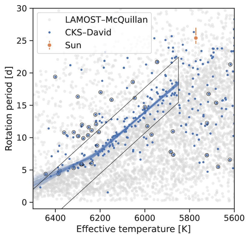
A change in slope along the long-period edge is observed in both the CKS and LAMOST samples (Figure 4), with an inflection point corresponding closely to the Kraft break at $\approx$ 6250 K, the point at which convective envelopes become vanishingly thin (Kraft, 1967). A piecewise linear fit to the ridge in the CKS sample confirmed that the inflection point occurs at $T_{\mathrm{eff}}$ = 6224 $\pm$ 24 K, where the uncertainty was estimated from Markov chain Monte Carlo (MCMC) sampling. This change in slope may be due to the fact that the convective turnover timescale, $\tau_{\mathrm{cz}}$, changes rapidly above 6250 K.

In the CKS sample, there also appears to be a clustering of stars above the ridge with $T_{\mathrm{eff}}$ $>6100$ K (seen most clearly in Figure 4). This cluster of points has a similar slope in the $T_{\mathrm{eff}}$–$P_{\mathrm{rot}}$ plane as the long-period pileup, and does not reside on the harmonic of the ridge line as one might expect if the periods were erroneously determined. A similar clustering of points is not observed in the LAMOST–McQuillan sample and is less pronounced or absent when substituting the CKS temperatures with $T_{\mathrm{eff}}$ from either Brewer & Fischer (2018) or Martinez et al. (2019), two studies that independently derived spectroscopic parameters from the CKS spectra. Further inspection of the stars in this cluster revealed that they have anomalously large $T_{\mathrm{eff}}$ discrepancies between the CKS and SPOCS catalogs, such that the SPOCS temperatures shift the stars onto the long-period pileup. We conclude that the temperatures for these stars in the CKS catalog are too high by $\gtrsim$ 100 K.

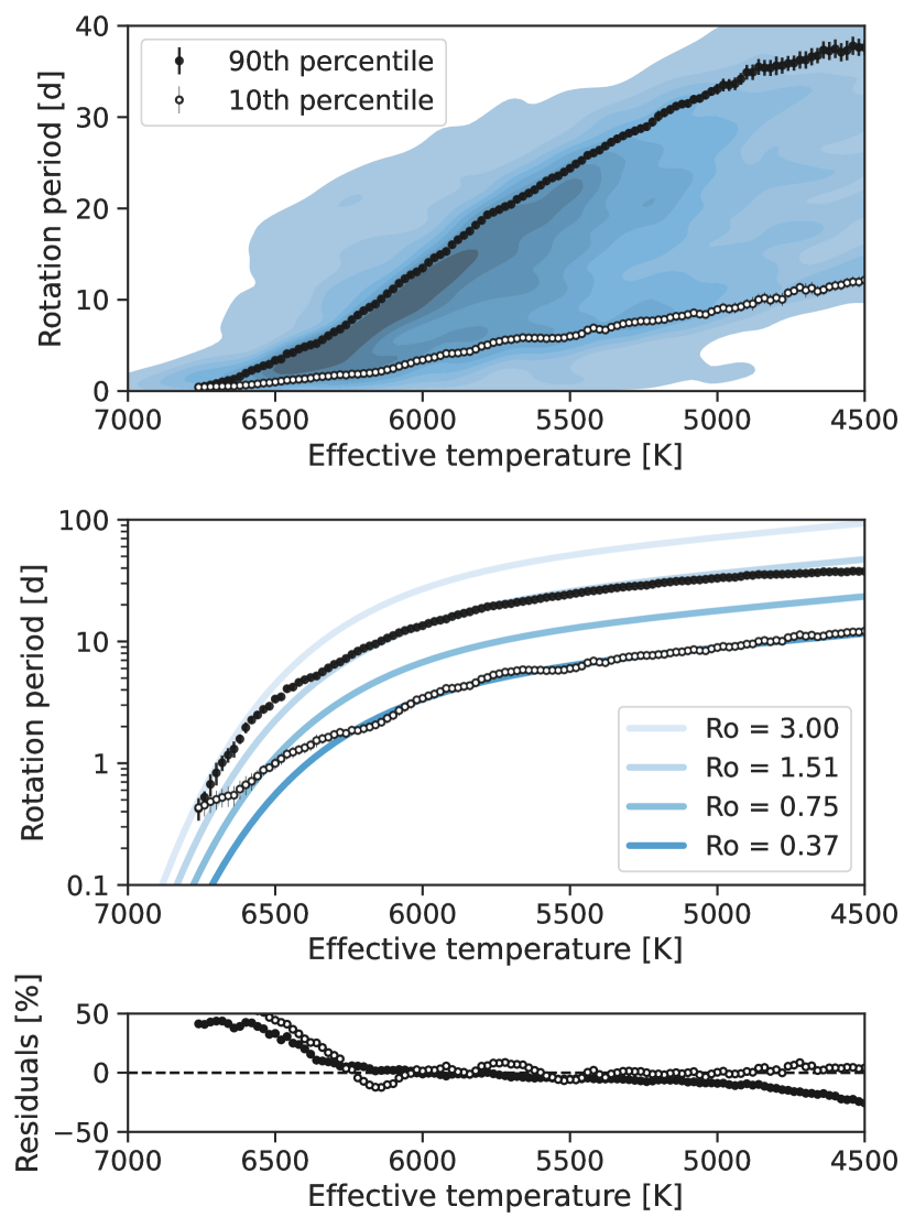
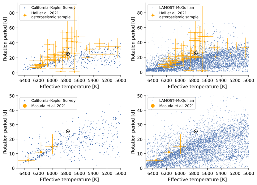
A secondary pileup at the short-period edge is also apparent, though less pronounced, in the $T_{\mathrm{eff}}$–$P_{\mathrm{rot}}$ distribution of the LAMOST–McQuillan sample. We verified through inspection that the secondary pileup does not lie along the $P_{\mathrm{rot}}$/2 harmonic line of the long-period pileup (see Appendix D). As shown in the middle panel of Figure 3 and the top panel of Figure 5, this secondary pileup is seen most clearly through applying Gaussian kernel density estimation (KDE), which was performed with the seaborn package (Waskom et al., 2017). The short-period pileup is also subtly apparent in the upper right panel of Figure 2, as well as scatter plots of the LAMOST–McQuillan sample, e.g. the second panel of Figure 1 and the bottom panels of Figures 7 and 8.

Figure 4: The $T_{\mathrm{eff}}$ –$P_{\mathrm{rot}}$ plane for the LAMOST–McQuillan sample (grey points) and the CKS sample (blue points) with periods sourced from David et al. (2021). The selection used to identify long-period pileup stars in the CKS sample is shown by the region enclosed by the black lines. Stars with $T_{\mathrm{eff}}$ differences $>100$ K between the CKS (Fulton & Petigura, 2018) and SPOCS (Brewer & Fischer, 2018) catalogs are shown by open black circles. The orange point indicates the Sun. Random draws from the MCMC chain of a piecewise linear fit to the CKS long-period pileup are shown by the blue lines. An inflection point in the long-period edge is apparent near $T_{\mathrm{eff}}$ = 6250 K.

3.2 Constant Rossby model

In the WMB model of van Saders et al. (2016, 2019), a star spins down until it reaches a critical Rossby number, at which point magnetic braking ceases. Since Rossby number is highly sensitive to temperature through its dependence on the convective turnover timescale ($\mathrm{Ro}=P_{\mathrm{rot}}/\tau_{\mathrm{cz}}$, where $\tau_{\mathrm{cz}}$ is the convective turnover timescale), this critical threshold corresponds to different rotation periods for stars of different $T_{\mathrm{eff}}$, leading to a pileup in the $T_{\mathrm{eff}}$-$P_{\mathrm{rot}}$ plane. Using a small sample of Kepler targets with rotation periods determined from brightness modulations, van Saders et al. (2016) proposed this threshold happens at a critical Rossby number of $\mathrm{Ro_{crit}}\sim\mathrm{Ro_{\odot}}$.

We tested the hypothesis that the long-period pileup observed in the LAMOST–McQuillan sample is compatible with the WMB model by fitting constant Rossby models to the $P_{\mathrm{rot}}$ boundary. For a given $T_{\mathrm{eff}}$, this model predicts $P_{\mathrm{rot}}$ as:

$$P_{\mathrm{rot}}(\mathrm{Ro},T_{\mathrm{eff}})=\mathrm{Ro}\times\tau_{\mathrm{cz}}(T_{\mathrm{eff}}),$$ (1)

where we used the equation for the convective turnover timescale (valid in the $T_{\mathrm{eff}}$ range of 3300 K$\lesssim T_{\mathrm{eff}}\lesssim$ 7000 K) presented in Cranmer & Saar (2011) from a fit to the zero-age main-sequence stellar models of Gunn et al. (1998):

$$\tau_{\mathrm{cz}}(T_{\mathrm{eff}})=314.24\exp\left[-\left(\frac{T_{\mathrm{eff}}}{1952.5\mathrm{K}}\right)-\left(\frac{T_{\mathrm{eff}}}{6250\mathrm{K}}\right)^{18}\right]\\ +0.002.$$ (2)

The above relation yields a convective turnover timescale for the Sun of $\tau_{\mathrm{cz,\odot}}=12.88$ d, leading to a Rossby number of $\mathrm{Ro_{\odot}}=1.97$ given the mean equatorial rotation period of $P_{\mathrm{rot,\odot}}=25.4$ d. For comparison, in the model grids used to create the population models in §3.3 the solar Rossby number is $\approx$2.16.

We approximated the long-period edge in the following manner. For 100 bootstrapped resamplings of the $T_{\mathrm{eff}}$ –$P_{\mathrm{rot}}$ distribution, leaving out 50% of the data for each bootstrapped sample, we computed the 90th percentile of $P_{\mathrm{rot}}$ values in overlapping $T_{\mathrm{eff}}$ bins with centers located every 20 K between 4000 K and 7000 K and half-widths of 100 K. The final long-period edge curve was then computed as the mean of the bootstrapped 90th percentile values. We found it was also necessary to omit stars with Ro $>$ 5/3 in this computation to match the long-period edge. We computed the 10th percentile curve and its uncertainty similarly, as an approximation to the lower boundary of the $T_{\mathrm{eff}}$-$P_{\mathrm{rot}}$ plane. We show these curves in relation to the full LAMOST–McQuillan sample and to constant Rossby models in Figure 5.

We performed an initial Levenberg-Marquardt non-linear least-squares fit of a constant Rossby model to the long-period edge with the curve_fit function in the scipy.optimize class to optimize the following likelihood:

$$\ln{p}(y|T_{\mathrm{eff}},T_{\mathrm{sys}},\sigma,\mathrm{Ro},f)=\\ -\frac{1}{2}\sum_{n}\left[\frac{(y_{n}-P_{\mathrm{rot}}(\mathrm{Ro},T_{\mathrm{eff}}+T_{\mathrm{sys}}))^{2}}{s_{n}^{2}}+\ln{(2\pi s_{n}^{2})}\right],$$ (3)

where

$$s_{n}^{2}=\sigma^{2}+f^{2}P_{\mathrm{rot}}(\mathrm{Ro},T_{\mathrm{eff}}+T_{\mathrm{sys}})^{2},$$ (4)

and $y_{n}$ is the value of a $P_{\mathrm{rot}}$ percentile curve in the $n$th $T_{\mathrm{eff}}$ bin. This is a Gaussian likelihood where the variance is underestimated by some fraction, $f$. Here $T_{\mathrm{sys}}$ is a constant to allow for a systematic offset between the data and the models used to calibrate the $\tau_{\mathrm{cz}}$ relation. This offset can equivalently be thought of as a correction to the data, or a correction to the model $T_{\mathrm{eff}}$ scale. We performed Markov chain Monte Carlo sampling (MCMC) of this likelihood with the emcee package (Foreman-Mackey et al., 2013, 2019) to estimate the mean and uncertainty of the critical Rossby number that best matches the long-period edge in the range of 5000 K$\lesssim T_{\mathrm{eff}}\lesssim$ 6250 K. We instantiated 32 walkers around the least-squares solution and sampled for $10^{5}$ steps, adopting uniform priors on Ro, $f$, and $T_{\mathrm{sys}}$ with ranges of (0.1,10), (0,10), and (-1000 K, 1000 K), respectively. Convergence was assessed by ensuring the chain length was at least 100 times longer than the chain autocorrelation lengths for each parameter. A similar analysis was performed for the 10th percentile curve, restricted in the range of 4500 K$\lesssim T_{\mathrm{eff}}\lesssim$ 5800 K where a constant Rossby model provides a reasonable fit.

We additionally fit the CKS long-period pileup (using three different homogeneous $T_{\mathrm{eff}}$ sources) and the H21 asteroseismic main-sequence sample, allowing for $T_{\mathrm{eff}}$ offsets in each data set (Table 1). For the CKS pileup stars and the LAMOST–McQuillan percentile curves, we assumed constant fractional $P_{\mathrm{rot}}$ uncertainties of 10%. To isolate the long-period pileup stars in the CKS sample, we selected a trapezoidal region using the condition $-0.0314~{}T_{\mathrm{eff}}+199.286<P_{\mathrm{rot}}<-0.0314~{}T_{\mathrm{eff}}+206.286$ (shown in Figure 4). We note that this selection is particular to the CKS $T_{\mathrm{eff}}$ scale and is not general. For the CKS sample, we additionally required $\log g~{}>~{}4$ and 5850 K $<~{}T_{\mathrm{eff}}~{}<$ 6500 K.

The constant Rossby model provides a reasonably good description of the LAMOST–McQuillan long-period edge in the $T_{\mathrm{eff}}$ range of $\approx$ 5000–6250 K, with fractional residuals $\lesssim 5\%$ over this range. Above and below this $T_{\mathrm{eff}}$ range we see clear and significant divergence from the constant Rossby model, such that the model under-predicts periods of hotter stars and over-predicts periods of cooler stars, possibly because the cooler stars have not had enough time to evolve to the critical Rossby number associated with weakened magnetic braking (see Figure 6 in van Saders et al., 2019).

In some cases, our constant Rossby fits to the long-period pileup prefer Rossby numbers lower than the Sun’s, in contrast with vS19. We caution against overinterpreting the specific $\mathrm{Ro_{crit}}$ values inferred here, and discuss our interpretations further in §4.2.

To further quantify the preference for $\mathrm{Ro_{crit}}$ $<$ $\mathrm{Ro_{\odot}}$ we performed non-linear least-squares fits of two models to the CKS long-period pileup and the LAMOST–McQuillan 90th percentile curve (both in the $T_{\mathrm{eff}}$ range of 5800–6250 K). The first model assumes $\mathrm{Ro_{crit}}$ = $\mathrm{Ro_{\odot}}$ and has one free parameter, a temperature offset added to the data. The second model assumes no temperature offset and allows $\mathrm{Ro_{crit}}$ to vary ($\mathrm{Ro_{crit}}$ being the only free parameter). The results of these fits are shown in Figure 6. We found that for the CKS sample, particularly when using the more precise temperatures from Fulton & Petigura (2018), that the $\Delta\chi^{2}$ between the $\mathrm{Ro_{crit}}$ = $\mathrm{Ro_{\odot}}$ and variable $\mathrm{Ro_{crit}}$ models was negligible. In other words, the $\mathrm{Ro_{crit}}$ = $\mathrm{Ro_{\odot}}$ model fits the data well with a $T_{\mathrm{eff}}$ shift of $\approx$ 70–140 K depending on the $T_{\mathrm{eff}}$ source used. For the LAMOST–McQuillan sample, there is weak support for the variable $\mathrm{Ro_{crit}}$ model. However, as shown in Appendix B, there is a strong systematic trend not adequately captured by a constant offset (i.e. a $T_{\mathrm{eff}}$-dependent $T_{\mathrm{eff}}$ offset) in the LAMOST temperatures when compared to other spectroscopic catalogs (particularly SPOCS). Correcting for these systematic trends weakens the support for the variable $\mathrm{Ro_{crit}}$ model, and we speculate that temperature systematics bias the $\mathrm{Ro_{crit}}$ inference procedure.

Figure 5: Top: Gaussian kernel density estimation of the LAMOST–McQuillan sample and the 10th and 90th $P_{\mathrm{rot}}$ percentiles (white and black points, respectively), computed as described in §3.2. Middle: The same 10th and 90th percentile curves shown in relation to constant Rossby curves. Bottom: Residuals from the median models resulting from the MCMC sampling. The fits depicted above do not include a $T_{\mathrm{eff}}$ offset.

Figure 6: Non-linear least-squares fits to the long-period pileup for a $\mathrm{Ro_{crit}}$ = $\mathrm{Ro_{\odot}}$ model with constant $T_{\mathrm{eff}}$ offset (orange) and a variable $\mathrm{Ro_{crit}}$ model with no $T_{\mathrm{eff}}$ offset (blue). The $\Delta\chi^{2}$ values printed in each panel are computed as $\chi^{2}_{\text{Ro}_{\text{crit}}=\text{Ro}_{\odot}}-\chi^{2}_{\Delta T_{eff}=0}$.

Table 1: Results of constant Rossby model fits.

Sample	$T_{\mathrm{eff}}$ range	Ro	f	$T_{\mathrm{sys}}$ (K)
Short-period pileup
LAMOST–McQuillan 10th $P_{\mathrm{rot}}$ pctl.	4500 K–5800 K	0.37 $\pm$ 0.02	0.011 $\pm$ 0.009	-46 $\pm$ 80
Long-period pileup
LAMOST–McQuillan 90th $P_{\mathrm{rot}}$ pctl.	5800 K–6250 K	1.4 $\pm$ 0.1	0.019 $\pm$ 0.015	-44 $\pm$ 43
CKS (CKS $T_{\mathrm{eff}}$)	5800 K–6250 K	1.77 $\pm$ 0.07	0.02 $\pm$ 0.01	70 $\pm$ 15
CKS (SPOCS $T_{\mathrm{eff}}$)	5800 K–6250 K	1.9 $\pm$ 0.1	0.12 $\pm$ 0.01	136 $\pm$ 23
CKS (M19 $T_{\mathrm{eff}}$)	5800 K–6250 K	1.6 $\pm$ 0.2	0.18 $\pm$ 0.02	-21 $\pm$ 42
Hall et al. (2021) main-sequence	5800 K–6250 K	1.9 $\pm$ 0.4	0.27 $\pm$ 0.05	29 $\pm$ 79

3.3 Comparison with theory

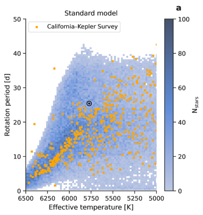
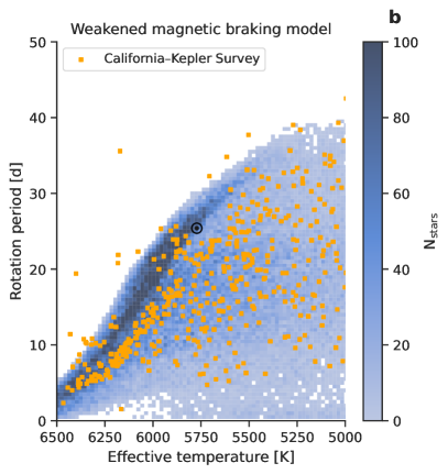
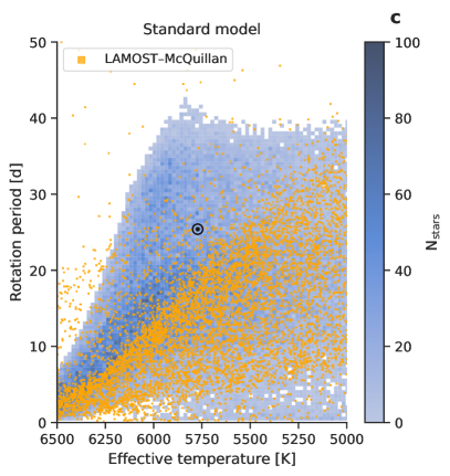
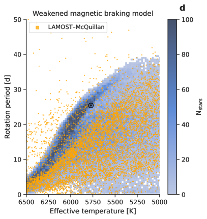
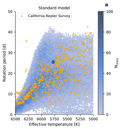
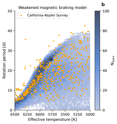
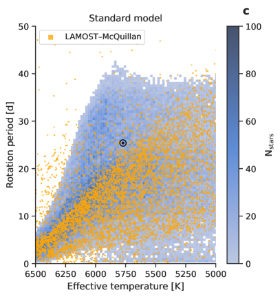
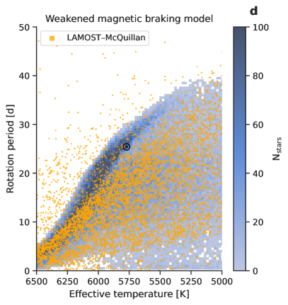
We compared the $T_{\mathrm{eff}}$–$P_{\mathrm{rot}}$ distribution of the CKS and LAMOST–McQuillan samples with the theoretical predictions of van Saders et al. (2019), which were updated for Hall et al. (2021) and utilized in that work. Those authors presented forward modeling simulations of the observed Kepler $P_{\mathrm{rot}}$ distribution including theoretical models of stellar angular momentum evolution (for both the standard spin-down and WMB scenarios), a galactic population model, and a prescribed observational selection function. For this exercise we selected main-sequence stars from the simulations using an evolutionary state flag, defining main-sequence stars as those with a He core mass fraction $<$0.0002. We did not apply a cut on Rossby number to the models to mimic a detection threshold, as one might expect if detectability is Ro-dependent. The issue of detection bias is discussed further in §4.1.

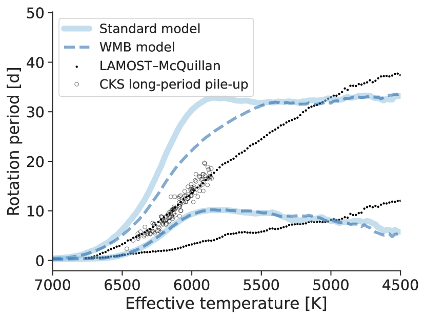
The theoretically predicted $T_{\mathrm{eff}}$–$P_{\mathrm{rot}}$ distributions of vS19 are shown in relation to the observations in Figure 7. Neither model satisfactorily matches the observations, though the WMB model more closely matches the long-period edge of F-type and early G-type stars. The specific WMB prescription of vS19 adopted a critical Rossby number of $\mathrm{Ro_{crit}}$ = 2.08 (using a different $\tau_{\mathrm{cz}}$ prescription than the one used here), leading to a pileup that is located at larger $P_{\mathrm{rot}}$ values (at fixed $T_{\mathrm{eff}}$) when compared to the observations, assuming no $T_{\mathrm{eff}}$ offset between the models and the data. Figure 8 shows the same models in relation to the data with constant $T_{\mathrm{eff}}$ offsets applied to the data, which are derived in §3.2. The $T_{\mathrm{eff}}$ offsets lead to better agreement between the data and models, although the long-period pileup in the LAMOST–McQuillan sample appears to overlay the models only for $T_{\mathrm{eff}}$ $\gtrsim 6000$ K, possibly due to strong $T_{\mathrm{eff}}$-dependent systematics in the LAMOST $T_{\mathrm{eff}}$ scale (see Appendix B).

To quantify the degree of agreement between the theoretical models and the LAMOST–McQuillan observations we computed the 10th and 90th percentile $P_{\mathrm{rot}}$ ranges of the standard and WMB models in overlapping $T_{\mathrm{eff}}$ bins, analogous to how the upper and lower boundaries of the observed $P_{\mathrm{rot}}$ distribution were found in §3.2. We computed the $\chi^{2}$ values between the observed upper edge and the 90th percentile ranges of the standard and WMB models, finding the WMB model is preferred with a $\Delta\chi^{2}=154$. Moreover, the WMB model better reproduces the slope of the observed long-period edge between 5300–6000 K (Figure 9).

While better agreement between the WMB model and observations might be achieved with stalling at a lower $\mathrm{Ro_{crit}}$, it is also possible that there are systematic offsets in the $T_{\mathrm{eff}}$ scales between the observations and models used in vS19, as well as differences in the computation of $\tau_{\mathrm{cz}}$. We also note that, while the models were computed using a simulated Kepler stellar population and selection function, the actual observed population and selection function of the LAMOST–McQuillan may be slightly different.

Shifting the LAMOST $T_{\mathrm{eff}}$ to higher values would bring the data into better agreement with the models, and in Appendix B we show the LAMOST $T_{\mathrm{eff}}$ are $\sim$50–100 K cooler than the other surveys considered here. In turn, it appears that the long-period edge for lower mass stars would be at higher $P_{\mathrm{rot}}$ than the models (i.e. the low-mass stars would be rotating more slowly than the model predictions). Such a discrepancy could result from different underlying populations between the models and the LAMOST–McQuillan sample, or a different normalization for the magnetic braking law. The models above employ a modified magnetic braking law that is scaled to match the rotation period of the Sun (see equations 1 & 2 of van Saders & Pinsonneault, 2013), with a normalization factor of $f_{K}=6.6$. A higher normalization factor would cause the low-mass stars to spin down more at fixed age.

Notably, both models fail to reproduce the observed short-period pileup, possibly due to the assumption of solid-body rotation in both models. At early times, Sun-like and low-mass stars are expected to have strong radial differential rotation due to their rapid collapse onto the main-sequence. The core and envelope at these times are thus assumed to be decoupled. However, the core and envelope are expected to couple on timescales of a few tens of million years for Sun-like stars (Denissenkov et al., 2010; Gallet & Bouvier, 2015; Lanzafame & Spada, 2015) or hundreds of million years for low-mass stars (Gallet & Bouvier, 2015; Lanzafame & Spada, 2015; Somers & Pinsonneault, 2016). When this happens, angular momentum can be transferred from the core to the envelope at a rate comparable to the rate at which angular momentum is lost via magnetized winds. Consequently, so-called “two-zone” models (MacGregor & Brenner, 1991) spin more rapidly than solid-body rotators at the same age. This hypothesis is discussed further in §4.3.

Figure 7: The $T_{\mathrm{eff}}$-$P_{\mathrm{rot}}$ plane for the CKS sample (top panels) and LAMOST sample (bottom panels) in comparison to the standard and WMB models (2-d histograms) presented in vS19. Shown here are stars with $\log g$ $>$ 4.1. Rotation periods for the CKS sample here are sourced from the David et al. (2021) compilation. The black symbol in each panel indicates the position of the Sun.

Figure 8: Same as Figure 7 with constant $T_{\mathrm{eff}}$ offsets applied to the data. Shifts of +111 K and +116 K are applied to the CKS and LAMOST $T_{\mathrm{eff}}$, respectively. The $T_{\mathrm{eff}}$ shifts originate from a least-squares fit of a $\mathrm{Ro_{crit}}$ = $\mathrm{Ro_{\odot}}$ curve (with a $T_{\mathrm{eff}}$ offset) to the long-period pileup (as described in §3.2).

Figure 9: Comparison of the theoretically predicted $T_{\mathrm{eff}}$–$P_{\mathrm{rot}}$ distribution of Kepler stars from vS19 (given by the 10th and 90th $P_{\mathrm{rot}}$ percentiles) with the same percentile ranges from the LAMOST–McQuillan sample (black points) and the CKS long-period pileup (open circles).

3.4 Comparison with literature surveys

H21 determined rotation periods for 91 main-sequence, asteroseismic Kepler targets from rotational splitting of asteroseismic oscillation frequencies. We found that the distribution of the asteroseismic sample in the $T_{\mathrm{eff}}$–$P_{\mathrm{rot}}$ plane approximately matches the pileup we observe, although the H21 sample appears shifted slightly to either higher $P_{\mathrm{rot}}$ or higher $T_{\mathrm{eff}}$ values relative to the ridge in the LAMOST–McQuillan sample while such an offset is either absent or not as apparent relative to the CKS sample. Such an offset could be due to differing spectroscopic temperature scales between the two studies, differing observational biases, or some combination of effects.

To assess the consistency of the $T_{\mathrm{eff}}$ scales between catalogs, we cross-matched the H21 sample with the LAMOST DR5 catalog and the CKS sample. We found a root mean square (RMS) of the residuals between the H21 and LAMOST DR5 $T_{\mathrm{eff}}$ measurements of 55 K, with a median offset of 41 K, such that the LAMOST $T_{\mathrm{eff}}$ scale is cooler, on average (see Appendix B). Similarly, we found excellent agreement between the $T_{\mathrm{eff}}$ scales of the CKS and H21 samples, with a median offset of 29 K (such that the CKS scale is hotter) and an RMS of 41 K. These offsets are modest, and do not account for non-linear systematics which may exist (particularly in the LAMOST $T_{\mathrm{eff}}$).

MPH21 inferred the $P_{\mathrm{rot}}$ distribution of 144 late-F/early-G dwarfs in the Kepler field from precise stellar radii and spectroscopically determined $v\sin i$. As with the asteroseismic sample, we compared the CKS and LAMOST–McQuillan samples with the results of those authors. We find that the long-period pileup we observe appears to overlap with the MPH21 data, within the uncertainties of those authors. We therefore consider it likely that the long-period pileup is the same feature, or an extension of the same feature, that was detected in the H21 and MPH21 studies.

Figure 10: Comparison of CKS (left column) and LAMOST–McQuillan samples (right column) with the H21 main-sequence asteroseismic sample (top row) and the MPH21 sample (bottom row) in the $T_{\mathrm{eff}}$–$P_{\mathrm{rot}}$ plane. The black point indicates the Sun. Note, the CKS, LAMOST, and H21 samples derive $T_{\mathrm{eff}}$ from distinct pipelines. In the top panels, constant offsets of -29 K and +41 K were added to the CKS and LAMOST $T_{\mathrm{eff}}$, respectively, based on comparisons to those stars with overlap in the H21 sample (see § 3.4 and Appendix B). Using LAMOST $T_{\mathrm{eff}}$, where it exists, for the H21 sample brings that sample into even closer agreement with the long-period pileup in the LAMOST-McQuillan sample.

3.5 Ages of stars on the long-period pileup

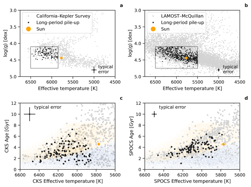
The WMB model predicts that hotter stars pile up on the long-period edge at younger ages, producing an age gradient across the edge. In Figure 11 we show the $T_{\mathrm{eff}}$-age distributions of stars on the ridge using ages from the CKS (Fulton & Petigura, 2018) and SPOCS (Brewer & Fischer, 2018) catalogs, where we use the trapezoidal selection described in §3.2 to select stars on the long-period pileup. Both catalogs derive spectroscopic parameters from the CKS spectra, but use different pipelines for both the spectroscopic parameters and the isochrone fitting.

In both cases, there appears to be an age gradient such that hotter stars are younger on average. However, such a trend is also expected in a sample of main-sequence stars as a natural consequence of the shorter main-sequence lifetimes of hotter, more massive stars. We also find that the dispersion in age is a sensitive function of $T_{\mathrm{eff}}$, with cooler stars on the ridge showing a broader range of ages. This observation could be due to cooler stars populating the ridge for longer periods of time (relative to hotter stars), the lower precision of isochrone ages for cooler stars, or some combination of the two effects.

We determined that 90% of the stars on the ridge have ages between 1.4–5.6 Gyr (using ages from the CKS catalog), or 2.3–5.9 Gyr (using SPOCS ages). These ranges are consistent with the range of ages observed in the H21 and MPH21 samples, as shown in Figure 11 of the latter reference. However, we note that systematic effects in surveys and theoretical models lead to large uncertainties in isochrone ages that are not necessarily represented by the reported age uncertainties. For example, it is curious that, when using SPOCS ages only $\sim$1% of the stars have ages $<$ 2 Gyr and that stars are concentrated at the upper age boundary for a given $T_{\mathrm{eff}}$ (Figure 11). In fact, there are only a handful of long-period pileup stars in the CKS sample with ages older than the age of the Sun (using CKS ages), and almost all of the pileup stars would be compatible with an age equal to or less than the Sun’s given the large age uncertainties.

In the WMB model, although wind-driven angular momentum losses cease, stars continue to evolve structurally which results in evolution in the moment of inertia and stellar spin, driven by expansion of the stars away from the main-sequence (van Saders et al., 2019). Stars reach $\mathrm{Ro_{crit}}$ $\approx$ 2 approximately halfway through their main-sequence lifetimes and remain there until the main-sequence turnoff. Thus, higher mass stars with shorter main-sequence lifetimes should show a smaller age spread on the long-period pileup relative to lower mass stars with longer main-sequence lifetimes. Though we have not quantified such an age-gradient, the data suggest that some stars spend several Gyr occupying the ridge with only modest evolution of their spin rates.

We additionally selected stars on the long-period pileup from the LAMOST–McQuillan sample by selecting stars with periods within 5% of the Ro = 1.3 curve (which traces the center of the highest density contour in Figure 3), 5500 K $<$ $T_{\mathrm{eff}}$ $<$ 6500 K, and 4.1 dex $<$ $\log g$ $<$ 4.75 dex. While ages for the LAMOST–Kepler sample are not available, the broad distribution of these stars in the spectroscopic H-R diagram supports the inference from the CKS sample that the long-period pileup is populated by stars with a broad range of ages (Figure 11). Interestingly, the solar $T_{\mathrm{eff}}$ and $\log g$ values appear to be wholly consistent with the distribution of long-period pileup stars. We discuss the Sun in context of the long-period pileup further in §4.5.

Figure 11: Above, H-R diagram placement of long-period pileup stars relative to the Sun and the CKS sample (a) and similarly for the LAMOST–McQuillan sample (b). Below, the $T_{\mathrm{eff}}$-age plane for CKS stars along the long-period pileup using isochrone ages from the CKS (c) and SPOCS (d) catalogs. The light shaded points represent predictions from the WMB model of vS19 for stars with Ro $<$ 2 (blue) and Ro $>$ 2 (orange). Note, panels (a), (c), and (d) all pertain to the CKS sample, whereas panel (b) relates to the LAMOST–McQuillan sample, for which homogeneous ages have not been published.

To further assess the evolutionary state of stars on the long-period pileup, we constructed a color-magnitude diagram (CMD) from the Gaia DR2 photometry and parallaxes for the Kepler field, the MMA14 and S21 rotation period catalogs, the H21 asteroseismic sample, and the CKS long-period pileup stars from this work (Figure 12). Stars with detected periods from rotational brightness modulations are primarily solar-type and lower-mass dwarfs, with a comparatively small number of subgiants. The S21 catalog contains more stars, in part due to the higher sensitivity to more slowly rotating, evolved stars, relative to MMA14. CKS stars on the long-period pileup clearly occupy a well-defined region of the upper main-sequence which overlaps well with the H21 asteroseismic sample.

Figure 12: Gaia DR2 color-magnitude diagram. In each panel, a 2-d histogram of all Kepler targets is shown in grayscale, with darker shades representing a higher number of targets in each cell. The estimated position of the Sun is indicated by the black point, based on the calibration of Casagrande & VandenBerg (2018). In the middle and right panels, the S21 targets with photometric rotation period detections are overplotted in orange. In the right panel, the CKS long-period pileup stars identified in this work are shown by blue points and a Gaussian kernel density estimation of the H21 asteroseismic sample is shown by blue contours. No reddening corrections were performed to the photometry in this figure.

3.6 Where do the pileups end?

It appears from Figures 3 and 7 that the number density of stars on the long-period pileup declines towards cooler $T_{\mathrm{eff}}$, as predicted by the WMB model (see Figure 13 of vS19). The number density of stars on the short-period pileup similarly declines towards cooler $T_{\mathrm{eff}}$. If the short-period pileup is due to core–envelope coupling, one might expect an opposite trend of increasing number density toward cooler $T_{\mathrm{eff}}$, since the core–envelope coupling timescales and hence the “stalled” braking phases are longer for lower-mass stars (Curtis et al., 2020). However, the observed $T_{\mathrm{eff}}$–$P_{\mathrm{rot}}$ distribution depends sensitively on the selection functions and observational biases inherent to both Kepler and the source of $T_{\mathrm{eff}}$ (e.g. LAMOST), which likely explains the observed number density trend.

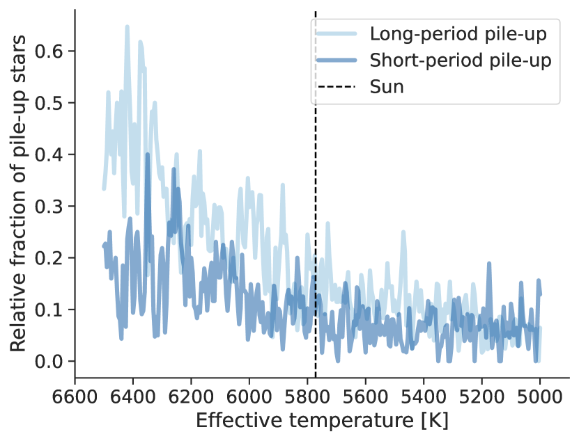
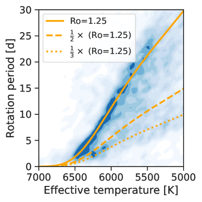
While it not clear whether or not these declines are astrophysical in nature, the result of the selection functions or observational biases inherent to Kepler or LAMOST, or some combination of effects, we attempted to characterize the extent of the pileups through the following approach. We found through inspection that constant Rossby curves of Ro=0.5 and Ro=1.3 (for the short- and long-period pileups, respectively) appear to describe the highest density contours found from Gaussian kernel density estimation of the LAMOST–McQuillan sample. In windows of 10 K width we measured the fraction of stars with periods within 1 d of each of the two constant Rossby curves, relative to the total number of stars in that $T_{\mathrm{eff}}$ window. We found that the relative fraction of stars on the long-period pileup declines rapidly between 6500 K and 5800 K, by more than half in that temperature range before plateauing at cooler $T_{\mathrm{eff}}$ (Figure 13). The relative fraction of stars on the short-period pileup declines more slowly, and below the temperature of the Sun, the relative fractions of stars on the two pileups are nearly equal. Thus, it is not yet clear if either pileup extends to temperatures cooler than $T_{\mathrm{eff,\odot}}$.

Figure 13: The relative fraction of stars on the long- and short-period pileups, in the LAMOST–McQuillan sample, in 10 K windows of $T_{\mathrm{eff}}$ (for stars with $\log g$ $>$4.1 dex).

4 Discussion

4.1 Detection biases

To this point, we have not addressed the detection biases inherent to Kepler rotation period catalogs. As periods become longer, they become more difficult to measure directly from Kepler time series. This is true for at least three reasons: (1) photometric variation amplitude declines with increasing Rossby number, (2) the existence of significant spot groups appears to be intermittent for high Rossby numbers, and (3) the observational baseline is finite. We note that the last point is not so important for Kepler’s long baseline ($\sim$1400 d), while the first two points are due to astrophysical reasons. This is important because, if a period detection threshold is Ro-dependent and the detection threshold Ro_thresh is close to the value $\mathrm{Ro_{crit}}$ at which WMB becomes important, then the location of the pileup in the catalogs considered here depends sensitively on how detectability depends on Ro. For example, if Ro_thresh is only slightly larger than $\mathrm{Ro_{crit}}$ and the long-period pileup has some non-negligible width in period space (due either to astrophysics or measurement error), then it’s possible the current data set only reveals the lower edge of the long-period pileup.

vS19 addressed detection biases in detail, finding that a threshold of Ro${}_{\mathrm{thresh}}\approx 2$ could reproduce the observed upper edge of the MMA14 $T_{\mathrm{eff}}$ –$P_{\mathrm{rot}}$ distribution. In this scenario, if $\mathrm{Ro_{thresh}}$ $\lesssim$ $\mathrm{Ro_{crit}}$, it becomes difficult to distinguish between the standard and WMB models in the MMA14 sample. However, those authors presented arguments that suggest detection bias is not solely responsible for producing the observed $T_{\mathrm{eff}}$ –$P_{\mathrm{rot}}$ distribution. We direct readers to §4.2 of that work for a summary of those arguments. Critically, we note here that while an Ro-dependent detection threshold may reproduce the upper edge of the $T_{\mathrm{eff}}$ –$P_{\mathrm{rot}}$ distribution, it would not be responsible for producing a pileup or overdensity at this edge. To our knowledge, there are no systematics of the rotation period catalogs considered here that would bias stars towards the detection threshold.

To understand whether the period detections on the long-period pileup are reliable, we examined the weight parameters published by MMA14. The weight, $w$, is a metric MMA14 designed to serve as a proxy for the reliability of a rotation period detection, based on a star’s autocorrelation function (ACF) properties and its position in $T_{\mathrm{eff}}$–$P_{\mathrm{rot}}$–LPH space, where LPH designates the local peak height of the ACF. Those authors selected $w>0.25$ for an acceptable compromise between real detections and false positives. In Figure 14, we show that the long-period pileup is apparent even for $w>0.3$, and we conclude that the majority of stars on the long-period pileup are likely to be genuine detections and not an artifact of some detection threshold.

Most importantly, two independent samples with different observational biases than the surveys considered here also appear to yield a pileup of stars at the long-period edge. These samples are the H21 Kepler asteroseismic sample, which measures rotation through asteroseismic mode splitting (discussed in §3.4), and the MPH21 sample of Kepler stars with Keck/HIRES spectroscopy, from which MPH21 inferred the peak of the $T_{\mathrm{eff}}$ –$P_{\mathrm{rot}}$ distribution using spectroscopically-determined $v\sin i$ and constraints on the stellar radii.

We do note, however, that we can not rule out the possibility that the long-period pileup is wider in period or Rossby space than we observe, with stars just above the pileup being undetected through rotational brightness modulations. Such a scenario might result if magnetic braking is gradually weakened once stars reach $\mathrm{Ro_{crit}}$, as opposed to ceasing entirely at $\mathrm{Ro_{crit}}$. However, even in this scenario there are observational constraints on the rate at which the braking index changes. If the braking index starts to decline as Ro approaches $\mathrm{Ro_{crit}}$ then there may be tension with the open cluster data. Additionally, if the pileup does have a broader width in Rossby number, the close agreement between our observations and the H21 and MPH21 samples suggests the true pileup width cannot be much larger than we observe.

Figure 14: The $T_{\mathrm{eff}}$ –$P_{\mathrm{rot}}$ distribution of the LAMOST–McQuillan sample for different weight thresholds (indicated above each panel) computed by MMA14.

4.2 Long-period behavior

The existence of a pileup of stars with a constant Rossby number is consistent with expectations from the WMB model of van Saders et al. (2016, 2019), as discussed in §3.2 and §3.3. The location of the long-period pileup coincides closely with the cluster of main-sequence stars with asteroseismic rotation rates determined by H21, as well as the peak of the period distribution inferred by MPH21 from combining $v\sin i$ and stellar radii. We suggest that these features are one and the same.

The modest differences between the long-period pileup we observe and the features observed by H21 and MPH21 might be explained by differing $T_{\mathrm{eff}}$ scales and differing observational biases of the samples. The present samples have rotation periods detected from photometric variations and, for a survey of finite baseline and sensitivity like Kepler, photometric rotation periods are harder to detect for slower rotators, smaller amplitude variations, and more stochastic variability patterns (see §4.1). The H21 asteroseismic sample and MPH21 sample, by comparison, are not biased against quiet, unspotted stars and are more likely to contain pileup stars that our sample may have missed.

In some cases, the $\mathrm{Ro_{crit}}$ values we inferred in §3.2 were smaller than the value of $\mathrm{Ro_{crit}}$ $\approx$ $\mathrm{Ro_{\odot}}$ $\approx$ 2 found by van Saders et al. (2016, 2019), sometimes with high statistical significance. We caution against overinterpreting the $\mathrm{Ro_{crit}}$ values inferred here, and enumerate below the ways in which the $\mathrm{Ro_{crit}}$ inference may be biased.

1. The $\tau_{\mathrm{cz}}$ relation adopted impacts the inferred $\mathrm{Ro_{crit}}$. We explored the $\tau_{\mathrm{cz}}$ formulae of Barnes & Kim (2010), Landin et al. (2010), and Amard et al. (2019), but these produce larger $\tau_{\mathrm{cz}}$ at fixed $T_{\mathrm{eff}}$ than the Cranmer & Saar (2011) relation, leading to even smaller inferred $\mathrm{Ro_{crit}}$ values. We also explored using a fit to the $\tau_{\mathrm{cz}}$ computed in vS19 for solar-metallicity stars, which produces a smaller $\tau_{\mathrm{cz}}$ at fixed $T_{\mathrm{eff}}$ than the Cranmer & Saar (2011) relation. This relation revises our $\mathrm{Ro_{crit}}$ estimates upwards by 15%.

2. While our $\mathrm{Ro_{crit}}$ inference procedure includes a constant $T_{\mathrm{eff}}$ offset between the data and the $\tau_{\mathrm{cz}}$ relation, it does not include any $T_{\mathrm{eff}}$-dependent offsets. In Appendix B, we show that the LAMOST $T_{\mathrm{eff}}$ appear to have a non-linear mapping to the other $T_{\mathrm{eff}}$ scales considered here. Perhaps not coincidentally, the LAMOST–McQuillan sample favors a $\mathrm{Ro_{crit}}$ that is the least compatible with other samples. We also note that the MCMC results for the LAMOST–McQuillan sample preferred the LAMOST $T_{\mathrm{eff}}$ to be shifted lower (Table 1), which is in inconsistent with our finding that the LAMOST $T_{\mathrm{eff}}$ are already lower than those from other spectroscopic surveys (Appendix B).

3. Defining the long-period pileup or edge is a choice that impacts the inferred value of $\mathrm{Ro_{crit}}$. For example, though we chose the 90th $P_{\mathrm{rot}}$ percentile in the LAMOST–McQuillan sample, vS19 chose the 95th percentile. Similarly, our boundary for the CKS long-period pileup was chosen subjectively.

It is evident from Figure 16 that the long-period pileup also coincides with a steep gradient in variability amplitude, such that a hidden population of pileup stars may lie just beyond the edge of detectability. This effect, in addition to the effects mentioned above, can further bias our inference of $\mathrm{Ro_{crit}}$ to lower values. Regardless of the biases mentioned above and the true value of $\mathrm{Ro_{crit}}$, the sample considered here clearly indicates that a pileup exists at the long-period edge for stars with $T_{\mathrm{eff}}$ $\gtrsim$ 5500 K. By construction, this pileup occurs at a Rossby number lower than that associated with a detection edge. In other words, the fact that we observe a pileup indicates that if WMB is assumed to be the cause, then $\mathrm{Ro_{crit}}$ $\lesssim$ $\mathrm{Ro_{thresh}}$, where $\mathrm{Ro_{thresh}}$ again is assumed to be a detection threshold.

We also note that the WMB model makes the simplistic assumption that magnetic braking ceases when Ro reaches $\mathrm{Ro_{crit}}$. However, it is possible that magnetic braking becomes gradually weaker, a scenario which would also lead to a pileup but may also cause such a pileup to have some intrinsic width which is not due to measurement uncertainties.

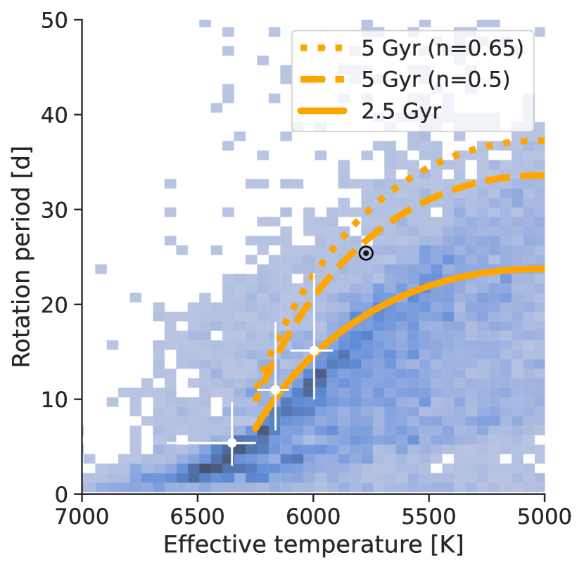
Our observation of a long-period pileup stands in contrast with recent rotation studies of solar analogs. do Nascimento et al. (2020) studied the rotation period distribution of 193 solar analogs, concluding that some solar-mass main-sequence stars appear to rotate significantly more slowly than the Sun, seemingly at odds with the WMB model. Additionally, Lorenzo-Oliveira et al. (2019) studied the $P_{\mathrm{rot}}$–age relation of solar twins observed by the Kepler mission, finding marginal statistical evidence in favor of a standard spin-down model over the WMB model. Those authors posited that if WMB takes place for Sun-like stars, it should happen at $\mathrm{Ro_{crit}}$ $\gtrsim 2.29$ or ages $\gtrsim$ 5.3 Gyr. A case study of an $\sim$8 Gyr solar twin further reinforced these conclusions (Lorenzo-Oliveira et al., 2020). By comparison, our findings provide support for the WMB model among stars that are slightly hotter than the Sun, but at $\mathrm{Ro_{crit}}$ $\lesssim$ $\mathrm{Ro_{\odot}}$ and at ages in the range of $\sim$2–6 Gyr. In contrast to the findings of those authors, we find that the long-period pileup lies far below an empirical 2.5 Gyr gyrochrone of C20 that is evolved forward to 5 Gyr for braking indices of $n=0.5$ or $n=0.65$ (Figure 15). This implies the braking index must drop to a much lower value at some time after 2.5 Gyr for Sun-like stars.

Figure 15: A 2-d histogram of the LAMOST–McQuillan $T_{\mathrm{eff}}$ –$P_{\mathrm{rot}}$ distribution compared to an empirical $\approx$ 2.5 Gyr hybrid cluster sequence from C20 (solid line). The dashed and dotted lines show the same sequence evolved forward to 5 Gyr assuming braking indices of $n=0.5$ (Skumanich-like spin-down) and $n=0.65$, which is favored by C20. For comparison, the white points indicate the peak of the $P_{\mathrm{rot}}$ distribution from MPH21 and the black point indicates the Sun.

4.3 Short-period behavior

Unlike the long-period pileup, the short-period pileup is not predicted by the WMB model or, more generally, any standard, solid-body braking model. However, this feature may also be due to an epoch of apparent stalling, albeit a temporary one since cluster studies demonstrate that stars continue to spin down beyond the short-period pileup. Works examining the $T_{\mathrm{eff}}$ –$P_{\mathrm{rot}}$ sequences of open clusters have found overlap between low-mass members in clusters of different ages (Agüeros et al., 2018; Curtis et al., 2019a, 2020), notably Praesepe (0.67 Gyr), NGC 6811 (1.4 Gyr), and NGC 752 (1.4 Gyr). In other words, the spin rates of low-mass stars appear to evolve very little in the time elapsed between the ages of those clusters. The short-period pileup we observe may be the manifestation of the same type of slowed spin evolution, but for stars of higher masses and younger ages than the cluster members in the above-mentioned works (since the pileup is observed at shorter periods relative to the Praesepe sequence).

Curtis et al. (2019a, 2020) proposed that the overlapping cluster sequences could be produced by a temporary epoch of stalled spin-down, caused either by (i) a reduction in the magnetic braking torque, or (ii) core–envelope momentum transfer which offsets the effect of magnetic braking (e.g. MacGregor & Brenner, 1991). In the core–envelope momentum transfer scenario angular momentum is exchanged between the envelope and the core on a characteristic timescale known as the core–envelope coupling timescale. The angular momentum transfer spins up the envelope, temporarily offsetting the spin-down via magnetic braking. Thus, in the core–envelope coupling scenario, spin evolution is slowed when the star’s age becomes comparable to the core–envelope coupling timescale. Theoretical predictions for the core–envelope coupling timescale for a solar-mass star range from 30–110 Myr (MacGregor & Brenner, 1991; Krishnamurthi et al., 1997; Bouvier, 2008; Irwin & Bouvier, 2009; Denissenkov et al., 2010; Gallet & Bouvier, 2015; Lanzafame & Spada, 2015; Somers & Pinsonneault, 2016; Spada & Lanzafame, 2020).

After a period of slowed spin-evolution, stars must resume spinning down as evidenced from studies of older open clusters. From open cluster data C20 estimated that solar-mass stars resume spin-down after an age of $\approx$ 230 Myr. Thus, if core–envelope coupling is responsible for delaying the spin-down of stars, and if the theoretical core–envelope coupling timescales are accurate, then we may expect Sun-like stars to experience slowed spin evolution between $\sim$100 Myr and $\sim$200 Myr.

Both the theoretically predicted core–envelope coupling timescale and the observationally inferred timescale for the resumption of spin-down are consistent with our observation that the short-period pileup is intermediate to the Pleiades (0.12 Gyr) and Praesepe (0.67 Gyr) cluster sequences. Furthermore, in order to match observations of rotation periods in young clusters, models require that the core–envelope coupling timescale increases towards lower stellar masses (e.g. Irwin et al., 2007; Denissenkov et al., 2010; Gallet & Bouvier, 2015), which provides a natural explanation for why this stalling occurs at older ages for lower-mass stars in C20.

We emphasize that the temporary epoch of slowed spin-down (also referred to as stalled magnetic braking) proposed by Curtis et al. (2019a, 2020) is not to be confused with the termination of magnetic braking that characterizes the WMB model of van Saders et al. (2016, 2019). The physical mechanisms thought to be responsible for each of these proposed stages of rotational evolution are distinct, though it is interesting that both the long- and short-period pileups seem to be well-described by curves of constant Rossby number. As mentioned above, one theory for the earlier stage of stalled spin-down is core–envelope coupling. Crucially, in the stalled spin-down phase, wind-driven angular momentum losses are not ceased but rather offset by the spin-up torque from core–envelope coupling. In contrast, in the WMB scenario, wind-driven angular momentum losses are proposed to cease ($dJ/dt$=0), with subsequent rotational evolution dictated by the changes in the moment of inertia.

Finally, we note that we regard the short-period pileup as less secure than the long-period pileup. Preliminary tests with other density estimation methods (Contardo et al., 2022) also reveal the short-period pileup, but further work is needed to better understand this feature. In Appendix D we show that the short-period pileup does not appear to be a harmonic of the long-period pileup, as one might expect if the periods on the short-period pileup were erroneously determined. However, the short-period pileup is primarily observed in the LAMOST–McQuillan sample, while it is unclear whether it is present in the LAMOST–Santos sample (see the rightmost panels of Figure 2). The differences between the MMA14 and S21 catalogs may provide an explanation for this observation. The latter catalog contains a much larger number of detections at longer rotation periods, and the higher sensitivity to more slowly rotating stars within the S21 may then make the short-period pileup appear weaker relative to the long-period pileup. This is as expected since open cluster observations suggest that the short-period pileup can not be a long-lived feature, while the long-period pileup appears to be much longer lived. Consequently, the S21 catalog may more accurately reflect the relative strengths of these two features.

4.4 Implications for the period gap

An unexplained feature of the Kepler rotation period distribution is the existence of a bimodal period distribution for dwarf stars of similar $T_{\mathrm{eff}}$. The effect was first noticed for M-dwarfs (McQuillan et al., 2013a), but was later shown to extend to $\sim$5000 K (Reinhold et al., 2013; McQuillan et al., 2014; Reinhold & Hekker, 2020), and even to $\sim$6500 K (Davenport, 2017).

McQuillan et al. (2013a, 2014) speculated that this period bimodality could originate from stellar populations of different ages, an explanation seemingly supported by a correlation between the strength of the bimodality and height above the galactic disk (Davenport & Covey, 2018). However, C20 demonstrated that cluster sequences cross the gap, invalidating the claim that the feature is caused at a specific age, as one might expect from a period of decreased star formation. Additionally, Gordon et al. (2021) found that the gap is observed across the many fields observed by the K2 mission, which is in tension with the star formation history hypothesis as different Galactic sight lines are expected to have different different star formation histories (for sufficiently large volumes).

An alternative explanation for the gap was proposed by Reinhold et al. (2019), who found that the dearth of stars with intermediate rotation periods is associated with a decrease in photometric variability. Consequently, those authors proposed that the period bimodality may be the result of a transition between spot- and faculae-dominated photospheres. In this scenario, the period gap is due to bright faculae canceling out the effects of dark star spots.

The short- and long-period pileups we examine here naturally produce a dearth of rotators at intermediate periods. This gap is the same period gap noticed by the authors mentioned above, as made apparent when comparing the LAMOST–McQuillan sample to the original MMA14 sample. Moreover, as seen in Figure 16, we recover the gradient in photometric variability across the gap pointed out by Reinhold et al. (2019). The photometric variability, as measured through the $R_{\mathrm{per}}$ metric published by MMA14, reaches a local minimum near the location of the gap. This supports the notion that the cause of the gap is due to changes in the stars themselves, rather than being the result of mixed stellar populations. However, the variability levels on both sides of the gap are not close to the detection limit, as evidenced by the fact that periods are securely detected for stars with similar properties at much lower $R_{\mathrm{per}}$ values. This would suggest that the period gap is not due solely to a detection issue, unless variability levels were to drop precipitously as stars approached the gap.

Gordon et al. (2021) proposed that the gap could instead be due to a period of accelerated spin-down immediately proceeding the stalling due to core–envelope coupling (such that stars evolve quickly through the gap and are rarely observed there). We can neither confirm nor reject this scenario, and we note that the gap is significantly emptier when using Gaia colors (Davenport & Covey, 2018; Gordon et al., 2021) compared to when using spectroscopic $T_{\mathrm{eff}}$ as we do here (see also Appendix C). Notably, if the short-period pileup is indeed due to core–envelope coupling, and the gap due to a period of accelerated spin-down after such a coupling episode, the observed gradient in photometric variability still requires a physical explanation.

Figure 16: The $T_{\mathrm{eff}}$–$P_{\mathrm{rot}}$ distribution of the LAMOST–McQuillan (left) and MMA14 samples color coded by the variability amplitude, $R_{\mathrm{per}}$. Black contours show Gaussian kernel density estimation of the plotted distributions, and the dashed line shows a constant Rossby curve of Ro = 0.5. The long- and short-period pileups are separated by a relative dearth of stars with intermediate rotation periods. A strong gradient in $R_{\mathrm{per}}$ is apparent across this gap, such that variability amplitude reaches a local minimum near the gap’s center.

4.5 Does the Sun reside on the long-period pileup?

It is unclear whether or not the Sun is a resident of the long-period pileup. From Fig. 2 it is clear that the long-period pileup extends to temperatures as cool as the Sun’s. If one assumes there are no systematic offsets between the spectroscopic $T_{\mathrm{eff}}$ scales considered here and that of the Sun, the Sun’s equatorial rotation period places it $\sim$5–7 days above the long-period pileup. This raises the question of how the Sun’s angular momentum has evolved to its current state, and whether WMB is a generic evolutionary phase.

If the Sun is indeed on the long-period pileup, it likely the presence of $T_{\mathrm{eff}}$ systematics and/or observational biases that obfuscate that fact. To place the Sun on the long-period pileup would require shifting the spectroscopic temperatures higher by 111 K for the CKS sample, 143 K for the SPOCS sample, or 116 K for the LAMOST sample. We also note that there are $T_{\mathrm{eff}}$-dependent systematics in the LAMOST $T_{\mathrm{eff}}$ that, if corrected for, would bring the LAMOST–McQuillan long-period pileup into closer agreement with a solar Rossby curve. Comparing the Sun to the H21 asteroseismic sample (Figure 3) seems to support the notion that the Sun may indeed reside on the long-period pileup, or very close to it, without the need for a large $T_{\mathrm{eff}}$ shift. This apears to be at odds with the notion that a $T_{\mathrm{eff}}$ shift alone can place the Sun on the long-period pileup, since the H21 and CKS temperature scales agree to within $\sim$30 K. However, it is still possible that there are $T_{\mathrm{eff}}$-dependend systematics in the temperature scales.

Furthermore, as discussed in §4.2, the H21 sample is less prone to detection bias which acts to censor stars with higher Ro and lower variability amplitudes in the samples considered here. As shown by Aigrain et al. (2015), the pipelines used to measure rotation periods from Kepler data would not be guaranteed to detect the solar rotation period. Regardless, it is clear from the comparisons in §3.4 that the long-period pileup can not be much broader (in $P_{\mathrm{rot}}$ or Rossby space) than we observe.

5 Conclusions

Our primary conclusions are summarized as follows:

1. We observe an overdensity at the long-period edge of the $T_{\mathrm{eff}}$-$P_{\mathrm{rot}}$ distribution of Kepler main-sequence stars with $T_{\mathrm{eff}}$ $\gtrsim$ 5500 K. We hypothesize that this pileup was previously obfuscated by imprecise $T_{\mathrm{eff}}$ estimates. Both the existence of the pileup and its obscuration by large $T_{\mathrm{eff}}$ errors were predicted by van Saders et al. (2019) as a consequence of weakened magnetic braking for stars with $M\gtrsim$1 $M_{\odot}$.

2. The long-period pileup is well-described by a constant Rossby number, with a critical value of $\mathrm{Ro_{crit}}~{}\lesssim~{}\mathrm{Ro_{\odot}}$, in the $T_{\mathrm{eff}}$ range of $\approx$ 5500-6250 K. The pileup is also populated by stars with a wide range of isochrone ages ($\sim$2–6 Gyr). A pileup of stars with a constant Rossby number and a broad range of ages is a prediction of the WMB model of van Saders et al. (2016, 2019). The precise value of $\mathrm{Ro_{crit}}$ is sensitive to $T_{\mathrm{eff}}$ scale shifts between observational data and the models used to compute $\tau_{\mathrm{cz}}$.

3. Comparison of the long-period pileup with empirical rotation sequences from open clusters implies that stars with $M\gtrsim 1$ $M_{\odot}$ pile up onto the ridge on a timescale $>$ 1 Gyr but $\lesssim$2.5 Gyr, compatible with the predictions of vS19. Using isochrone ages for a sample of exoplanet hosts on the long-period pileup suggests that stars slightly hotter than the Sun may populate the pileup until an age of $\sim$6 Gyr.

4. It is yet unclear whether the Sun resides on the long-period pileup or has already evolved through it. Offsets of $\approx$110–140 K between the observational and theoretical $T_{\mathrm{eff}}$ scales would place the long-period pileup at Rossby numbers consistent with other literature values of the location of the WMB transition. If the Sun has evolved through the pileup, there is some modest tension with the Sun’s age and the ages of the oldest stars on the pileup; some of the cooler long-period pileup stars in the CKS sample are both more massive and older than the Sun, which contradicts the expectation from the WMB model that hotter stars spend a shorter period of time on the pileup. However, this tension might be simply explained by inaccurate isochrone ages.

5. We tentatively detect a secondary overdensity of stars at the short-period edge of the $T_{\mathrm{eff}}$-$P_{\mathrm{rot}}$ plane. This overdensity appears to be less prominent than the long-period overdensity, possibly indicating that the short-period pileup is shorter-lived, $\mathcal{O}(10^{8}\text{yr})$, relative to the long-period pileup ($>10^{9}$ yr). The short-period pileup appears to be intermediate to the empirical Pleiades (0.12 Gyr) and Praesepe (0.67 Gyr) open cluster sequences and may result from a temporary epoch of stalled spin-down due to core–envelope coupling, as proposed by C20. The short-period pileup can also be fit with a constant Rossby model, though over a range of $T_{\mathrm{eff}}$ that differs from that of the long-period pileup.

6. The number density of stars on the long-period pileup declines with $T_{\mathrm{eff}}$, in line with predictions from the WMB hypothesis, though it remains unclear whether this observation is due to astrophysics, the Kepler selection function, observational biases, or some combination of effects. The relative fraction of stars on the long-period pile up declines by a factor of $\sim$2 between $\sim$6200 K and $\sim$5800 K.

7. We find tentative evidence for an age-gradient along the long-period pileup, such that hotter stars on the ridge are younger on average. Relatedly, the age dispersion along the ridge is non-uniform as a function of temperature, with hotter stars showing a smaller dispersion. This observation suggests that hotter stars reside on the long-period pileup for a shorter period of time relative to cooler stars. These observations are in accordance with predictions from the WMB model, which predicts that stars of different masses spend an approximately equal fraction of their respective main-sequence lifetimes on the long-period pileup. However, a more careful analysis is required to conclusively show these observations are not due to the intrinsic age gradient expected among a sample of main sequence stars with different masses and the higher isochrone age uncertainties associated with cooler stars.

8. The existence of the long-period pileup limits the utility of gyrochronology for the hottest stars with convective envelopes, as stellar spin-down appears to stall on the pileup. For example, a Sun-like star may spend several Gyr evolving through the long-period pileup. Authors using gyrochronology as a means of age-dating a field dwarf star with $T_{\mathrm{eff}}$ $\gtrsim$ 5500 K (and possibly cooler $T_{\mathrm{eff}}$ as well) should take care to assess whether that star resides on the long-period edge, in which case the uncertainty on the age may be larger than current gyrochronology calibrations imply.

9. An increasing number of open clusters are being discovered by searching for a clustering of rotation periods along a slow-rotator sequence in the $T_{\mathrm{eff}}$ –$P_{\mathrm{rot}}$ or color–$P_{\mathrm{rot}}$ plane. However, the long-period pile up discovered here can mimic a slow-rotator sequence in a small sample of unassociated stars with different ages and precisely measured temperatures and rotation periods. This is clearly demonstrated by the CKS sample in the right-hand panel of Figure 1. Taken out of context, this sample resembles a group of coeval stars with a slow-rotator sequence. The discovery of pileups in stellar rotation periods therefore has consequences for open cluster studies. When an overdensity or ridge is present in the rotation period distribution of a stellar population, care must be taken to ensure that it is not caused by WMB or core–envelope coupling before assuming that population is coeval and using the overdensity to age-date it.

The code and data tables required to reproduce the figures and analysis presented here are publicly available through GitHub. The data tables are also available through Zenodo.

Appendix A Comparison of temperature-period distributions

In Figure 17, we show how the $T_{\mathrm{eff}}$–$P_{\mathrm{rot}}$ distribution of the CKS sample changes when sourcing $T_{\mathrm{eff}}$ and $P_{\mathrm{rot}}$ from different, homogeneous catalogs in the literature. The sharpness of the long-period pileup appears to be determined primarily by the source of $T_{\mathrm{eff}}$, rather than $P_{\mathrm{rot}}$. The CKS-Gaia catalog (Fulton & Petigura, 2018) appears to offer the highest internal precision.

Figure 17: Comparison of the $T_{\mathrm{eff}}$–$P_{\mathrm{rot}}$ distribution for the CKS sample using rotation periods and $T_{\mathrm{eff}}$ from the sources indicated by the axes labels.

Appendix B Comparison of spectroscopic temperature scales

In Figure 18 we compare temperatures between the LAMOST DR5 catalog (Xiang et al., 2019) and temperatures from other surveys. We find that the LAMOST $T_{\mathrm{eff}}$ scale is consistently cooler than other surveys by $\sim$20–80 K, with the exception of the MMA14 study which sourced photometric $T_{\mathrm{eff}}$ estimates from the KIC (Brown et al., 2011). A LAMOST $T_{\mathrm{eff}}$ scale which is systematically cooler provides support to the notion that $\mathrm{Ro_{crit}}$ determined from LAMOST temperatures will be systematically underestimated.

Figure 18: Comparison of $T_{\mathrm{eff}}$ estimates from different catalogs: LAMOST (Xiang et al., 2019), CKS (Fulton & Petigura, 2018), SPOCS (Brewer & Fischer, 2018), M19 (Martinez et al., 2019), MMA14, and H21.

Appendix C The Gaia color–period plane

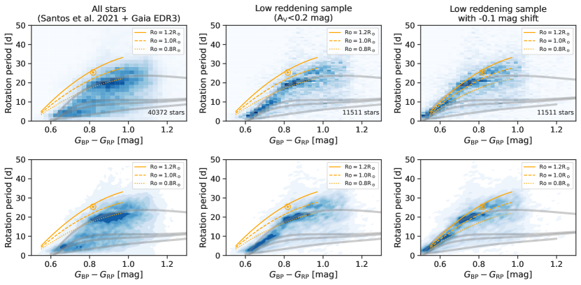
Given that the long-period pileup was previously obscured by imprecise $T_{\mathrm{eff}}$ measurements, we explored whether the feature could be recovered using the high-precision photometric colors provided by the Gaia mission (Gaia Collaboration et al., 2016). We cross-matched the MMA14 and S21 samples with Gaia EDR3 (Gaia Collaboration et al., 2021) using a 1 arcsec search radius and the astroquery package (Ginsburg et al., 2019). We retrieved reddening estimates for each target by querying the Bayestar19 3D dust map using the dustmaps package (Green, 2018; Green et al., 2019). We then compared the ($G_{BP}-G_{RP}$)–$P_{\mathrm{rot}}$ distribution with constant Rossby curves. For this exercise, we used the empirically calibrated $\tau_{\mathrm{cz}}$ relation of Corsaro et al. (2021), who presented $\tau_{\mathrm{cz}}$ as a quadratic function of Gaia $G_{BP}-G_{RP}$ color using the Kepler LEGACY asteroseismic sample as calibrators. We found that the long-period pileup is clearly visible in the ($G_{BP}-G_{RP}$)–$P_{\mathrm{rot}}$ plane once stars with high reddening ($A_{V}>0.2$) are excluded. In order to match a curve of constant Rossby number, given by $\mathrm{Ro}=\mathrm{Ro_{\odot}}=0.496$ on the Corsaro et al. (2021) scale, we found that a $\approx$-0.1 mag shift to the Gaia colors of the data was required (or, equivalently, a +0.1 mag shift applied to the constant Rossby curve). While there is no justification for such a large shift, it may indicate the presence of a systematic offset in the $\tau_{\mathrm{cz}}$ relation. We also note that we do not have an explanation for why the solar value Rossby curve does not pass through the Sun.

We note that the morphology of the color–period distribution appears to be different between the Gaia–McQuillan and Gaia–Santos catalogs, with the Gaia–Santos distribution presenting a break near $G_{BP}-G_{RP}=0.7$. This break is not apparent in the Gaia–McQuillan sample. Similar behavior is seen in $T_{\mathrm{eff}}$ –$P_{\mathrm{rot}}$ plane, as shown in Figure 2, suggesting the origin of the discontinuity is in the rotation periods rather than the temperatures or colors. At present, we do not have a satisfactory explanation for this behavior, though we note that the S21 catalog employed various time series filters which might introduce systematic artifacts.

Figure 19: The color–$P_{\mathrm{rot}}$ plane for the MMA14 sample in relation to a curve of constant Rossby number (orange dashed curve, $\mathrm{Ro}=\mathrm{Ro}_{\odot}=0.496$) from the empirical $\tau_{\mathrm{cz}}$ calibration of Corsaro et al. (2021), which is valid in the color range $0.55<(G_{\mathrm{BP}}\textendash G_{\mathrm{RP}})<0.97$. The top rows show 2–d histograms of the probability density for the entire sample (left), a subsample with low reddening (middle), and the same low reddening subsample with a -0.1 mag color shift applied to the data and cluster sequences. Each panel in the bottom row shows a Gaussian kernel density estimation of the respective panel above. The orange point in each panel represents the position of the Sun, using the estimated Gaia color of Casagrande & VandenBerg (2018). The grey lines indicate empirical cluster sequences derived in C20. From top to bottom, the cluster sequences are Pleiades (0.12 Gyr), Praesepe (0.67 Gyr), NGC 6811 (1 Gyr), and NGC 6819 + Ruprecht 147 (2.5 Gyr).

Figure 20: The same as Figure 19 but for the S21 sample.

Appendix D Confounding scenarios for the short-period pileup

Here we consider the possibility that there is only one astrophysical overdensity in the true $T_{\mathrm{eff}}$ –$P_{\mathrm{rot}}$ distribution, the long-period pileup, and other features in the observed $T_{\mathrm{eff}}$ –$P_{\mathrm{rot}}$ distribution appear at period harmonics of this feature due to the difficult problem of reliable, automated rotation period measurement for large samples of stars. Figure 21 shows a Gaussian kernel density estimation of the LAMOST–McQuillan $T_{\mathrm{eff}}$ –$P_{\mathrm{rot}}$ distribution for stars with $\log g$ $>$ 4.1. The short-period pileup is observed in this sample, particularly for $T_{\mathrm{eff}}$ $>$ 6000 K. We found through inspection a constant Rossby curve that traces the long-period pileup. Taking this curve and dividing the periods by factors of 2 and 3, we find that neither resulting curve satisfactorily matches the short-period pileup, though they both bracket the feature seen through density estimation. We interpret this as evidence that the short-period pileup is not simply due to measurement error, although we have not definitively ruled out that scenario.

Figure 21: Gaussian kernel density estimation of the $T_{\mathrm{eff}}$ –$P_{\mathrm{rot}}$ distribution in the LAMOST–McQuillan sample for stars with $\log g$ $>$ 4.1. A curve of constant Rossby number is shown by the solid line. The $P_{\mathrm{rot}}$/2 and $P_{\mathrm{rot}}$/3 harmonics of this curve are shown by the dashed and dotted lines, respectively. The short-period pileup is seen near the short-period edge, particularly for $T_{\mathrm{eff}}$ $>$ 6000 K. The short-period pileup does not appear to be simply a harmonic of the long-period pileup, as one might expect if the periods for the stars in the short-period pileup were erroneously determined.

References

- Agüeros et al. (2018) Agüeros, M. A., Bowsher, E. C., Bochanski, J. J., et al. 2018, ApJ, 862, 33, doi: 10.3847/1538-4357/aac6ed
- Ahumada et al. (2020) Ahumada, R., Prieto, C. A., Almeida, A., et al. 2020, ApJS, 249, 3, doi: 10.3847/1538-4365/ab929e
- Aigrain et al. (2015) Aigrain, S., Llama, J., Ceillier, T., et al. 2015, MNRAS, 450, 3211, doi: 10.1093/mnras/stv853
- Amard et al. (2019) Amard, L., Palacios, A., Charbonnel, C., et al. 2019, A&A, 631, A77, doi: 10.1051/0004-6361/201935160
- Angus et al. (2015) Angus, R., Aigrain, S., Foreman-Mackey, D., & McQuillan, A. 2015, MNRAS, 450, 1787, doi: 10.1093/mnras/stv423
- Angus et al. (2018) Angus, R., Morton, T., Aigrain, S., Foreman-Mackey, D., & Rajpaul, V. 2018, MNRAS, 474, 2094, doi: 10.1093/mnras/stx2109
- Angus et al. (2019) Angus, R., Morton, T. D., Foreman-Mackey, D., et al. 2019, AJ, 158, 173, doi: 10.3847/1538-3881/ab3c53
- Astropy Collaboration et al. (2013) Astropy Collaboration, Robitaille, T. P., Tollerud, E. J., et al. 2013, A&A, 558, A33, doi: 10.1051/0004-6361/201322068
- Astropy Collaboration et al. (2018) Astropy Collaboration, Price-Whelan, A. M., SipH ocz, B. M., et al. 2018, AJ, 156, 123, doi: 10.3847/1538-3881/aabc4f
- Bahcall et al. (1995) Bahcall, J. N., Pinsonneault, M. H., & Wasserburg, G. J. 1995, Reviews of Modern Physics, 67, 781, doi: 10.1103/RevModPhys.67.781
- Barnes (2003) Barnes, S. A. 2003, ApJ, 586, 464, doi: 10.1086/367639
- Barnes (2007) —. 2007, ApJ, 669, 1167, doi: 10.1086/519295
- Barnes (2010) —. 2010, ApJ, 722, 222, doi: 10.1088/0004-637X/722/1/222
- Barnes & Kim (2010) Barnes, S. A., & Kim, Y.-C. 2010, ApJ, 721, 675, doi: 10.1088/0004-637X/721/1/675
- Blanton et al. (2017) Blanton, M. R., Bershady, M. A., Abolfathi, B., et al. 2017, AJ, 154, 28, doi: 10.3847/1538-3881/aa7567
- Borucki et al. (2010) Borucki, W. J., Koch, D., Basri, G., et al. 2010, Science, 327, 977, doi: 10.1126/science.1185402
- Bouvier (2008) Bouvier, J. 2008, A&A, 489, L53, doi: 10.1051/0004-6361:200810574
- Brewer & Fischer (2018) Brewer, J. M., & Fischer, D. A. 2018, ApJS, 237, 38, doi: 10.3847/1538-4365/aad501
- Brown et al. (2011) Brown, T. M., Latham, D. W., Everett, M. E., & Esquerdo, G. A. 2011, AJ, 142, 112, doi: 10.1088/0004-6256/142/4/112
- Casagrande & VandenBerg (2018) Casagrande, L., & VandenBerg, D. A. 2018, MNRAS, 479, L102, doi: 10.1093/mnrasl/sly104
- Contardo et al. (2022) Contardo, G., Hogg, D. W., Hunt, J. A. S., Peek, J. E. G., & Chen, Y.-C. 2022, arXiv e-prints, arXiv:2201.10674. https://arxiv.org/abs/2201.10674
- Corsaro et al. (2021) Corsaro, E., Bonanno, A., Mathur, S., et al. 2021, A&A, 652, L2, doi: 10.1051/0004-6361/202141395
- Cranmer & Saar (2011) Cranmer, S. R., & Saar, S. H. 2011, ApJ, 741, 54, doi: 10.1088/0004-637X/741/1/54
- Curtis et al. (2019a) Curtis, J. L., Agüeros, M. A., Douglas, S. T., & Meibom, S. 2019a, ApJ, 879, 49, doi: 10.3847/1538-4357/ab2393
- Curtis et al. (2019b) Curtis, J. L., Agüeros, M. A., Mamajek, E. E., Wright, J. T., & Cummings, J. D. 2019b, AJ, 158, 77, doi: 10.3847/1538-3881/ab2899
- Curtis et al. (2020) Curtis, J. L., Agüeros, M. A., Matt, S. P., et al. 2020, ApJ, 904, 140, doi: 10.3847/1538-4357/abbf58
- Davenport (2017) Davenport, J. R. A. 2017, ApJ, 835, 16, doi: 10.3847/1538-4357/835/1/16
- Davenport & Covey (2018) Davenport, J. R. A., & Covey, K. R. 2018, ApJ, 868, 151, doi: 10.3847/1538-4357/aae842
- David et al. (2021) David, T. J., Contardo, G., Sandoval, A., et al. 2021, AJ, 161, 265, doi: 10.3847/1538-3881/abf439
- De Cat et al. (2015) De Cat, P., Fu, J. N., Ren, A. B., et al. 2015, ApJS, 220, 19, doi: 10.1088/0067-0049/220/1/19
- Denissenkov et al. (2010) Denissenkov, P. A., Pinsonneault, M., Terndrup, D. M., & Newsham, G. 2010, ApJ, 716, 1269, doi: 10.1088/0004-637X/716/2/1269
- do Nascimento et al. (2020) do Nascimento, J. D., J., de Almeida, L., Velloso, E. N., et al. 2020, ApJ, 898, 173, doi: 10.3847/1538-4357/ab9c16
- Douglas et al. (2016) Douglas, S. T., Agüeros, M. A., Covey, K. R., et al. 2016, ApJ, 822, 47, doi: 10.3847/0004-637X/822/1/47
- Douglas et al. (2017) Douglas, S. T., Agüeros, M. A., Covey, K. R., & Kraus, A. 2017, ApJ, 842, 83, doi: 10.3847/1538-4357/aa6e52
- Douglas et al. (2019) Douglas, S. T., Curtis, J. L., Agüeros, M. A., et al. 2019, ApJ, 879, 100, doi: 10.3847/1538-4357/ab2468
- Dressing & Charbonneau (2013) Dressing, C. D., & Charbonneau, D. 2013, ApJ, 767, 95, doi: 10.1088/0004-637X/767/1/95
- Foreman-Mackey (2016) Foreman-Mackey, D. 2016, The Journal of Open Source Software, 1, 24, doi: 10.21105/joss.00024
- Foreman-Mackey et al. (2013) Foreman-Mackey, D., Hogg, D. W., Lang, D., & Goodman, J. 2013, PASP, 125, 306, doi: 10.1086/670067
- Foreman-Mackey et al. (2019) Foreman-Mackey, D., Farr, W., Sinha, M., et al. 2019, The Journal of Open Source Software, 4, 1864, doi: 10.21105/joss.01864
- Fulton & Petigura (2018) Fulton, B. J., & Petigura, E. A. 2018, AJ, 156, 264, doi: 10.3847/1538-3881/aae828
- Gaia Collaboration et al. (2016) Gaia Collaboration, Prusti, T., de Bruijne, J. H. J., et al. 2016, A&A, 595, A1, doi: 10.1051/0004-6361/201629272
- Gaia Collaboration et al. (2018) Gaia Collaboration, Brown, A. G. A., Vallenari, A., et al. 2018, A&A, 616, A1, doi: 10.1051/0004-6361/201833051
- Gaia Collaboration et al. (2021) —. 2021, A&A, 649, A1, doi: 10.1051/0004-6361/202039657
- Gallet & Bouvier (2015) Gallet, F., & Bouvier, J. 2015, A&A, 577, A98, doi: 10.1051/0004-6361/201525660
- Garraffo et al. (2016) Garraffo, C., Drake, J. J., & Cohen, O. 2016, A&A, 595, A110, doi: 10.1051/0004-6361/201628367
- Ginsburg et al. (2019) Ginsburg, A., Sipőcz, B. M., Brasseur, C. E., et al. 2019, AJ, 157, 98, doi: 10.3847/1538-3881/aafc33
- Gordon et al. (2021) Gordon, T. A., Davenport, J. R. A., Angus, R., et al. 2021, ApJ, 913, 70, doi: 10.3847/1538-4357/abf63e
- Green (2018) Green, G. 2018, The Journal of Open Source Software, 3, 695, doi: 10.21105/joss.00695
- Green et al. (2019) Green, G. M., Schlafly, E., Zucker, C., Speagle, J. S., & Finkbeiner, D. 2019, ApJ, 887, 93, doi: 10.3847/1538-4357/ab5362
- Gunn et al. (1998) Gunn, A. G., Mitrou, C. K., & Doyle, J. G. 1998, MNRAS, 296, 150, doi: 10.1046/j.1365-8711.1998.01347.x
- Hall et al. (2021) Hall, O. J., Davies, G. R., van Saders, J., et al. 2021, Nature Astronomy, 5, 707, doi: 10.1038/s41550-021-01335-x
- Hathaway (2015) Hathaway, D. H. 2015, Living Reviews in Solar Physics, 12, 4, doi: 10.1007/lrsp-2015-4
- Howell et al. (2014) Howell, S. B., Sobeck, C., Haas, M., et al. 2014, PASP, 126, 398, doi: 10.1086/676406
- Huber et al. (2014) Huber, D., Silva Aguirre, V., Matthews, J. M., et al. 2014, ApJS, 211, 2, doi: 10.1088/0067-0049/211/1/2
- Hunter (2007) Hunter, J. D. 2007, Computing in Science and Engineering, 9, 90, doi: 10.1109/MCSE.2007.55
- Irwin & Bouvier (2009) Irwin, J., & Bouvier, J. 2009, in The Ages of Stars, ed. E. E. Mamajek, D. R. Soderblom, & R. F. G. Wyse, Vol. 258, 363–374, doi: 10.1017/S1743921309032025
- Irwin et al. (2007) Irwin, J., Hodgkin, S., Aigrain, S., et al. 2007, MNRAS, 377, 741, doi: 10.1111/j.1365-2966.2007.11640.x
- Jones et al. (2001–) Jones, E., Oliphant, T., Peterson, P., et al. 2001–, SciPy: Open source scientific tools for Python. http://www.scipy.org/
- Jönsson et al. (2020) Jönsson, H., Holtzman, J. A., Allende Prieto, C., et al. 2020, AJ, 160, 120, doi: 10.3847/1538-3881/aba592
- Kawaler (1988) Kawaler, S. D. 1988, ApJ, 333, 236, doi: 10.1086/166740
- Kluyver et al. (2016) Kluyver, T., Ragan-Kelley, B., Pérez, F., et al. 2016, in Positioning and Power in Academic Publishing: Players, Agents and Agendas, ed. F. Loizides & B. Schmidt, IOS Press, 87 – 90
- Kraft (1967) Kraft, R. P. 1967, ApJ, 150, 551, doi: 10.1086/149359
- Krishnamurthi et al. (1997) Krishnamurthi, A., Pinsonneault, M. H., Barnes, S., & Sofia, S. 1997, ApJ, 480, 303, doi: 10.1086/303958
- Landin et al. (2010) Landin, N. R., Mendes, L. T. S., & Vaz, L. P. R. 2010, A&A, 510, A46, doi: 10.1051/0004-6361/200913015
- Lanzafame & Spada (2015) Lanzafame, A. C., & Spada, F. 2015, A&A, 584, A30, doi: 10.1051/0004-6361/201526770
- Lorenzo-Oliveira et al. (2020) Lorenzo-Oliveira, D., Meléndez, J., Ponte, G., & Galarza, J. Y. 2020, MNRAS, 495, L61, doi: 10.1093/mnrasl/slaa057
- Lorenzo-Oliveira et al. (2019) Lorenzo-Oliveira, D., Meléndez, J., Yana Galarza, J., et al. 2019, MNRAS, 485, L68, doi: 10.1093/mnrasl/slz034
- Luger et al. (2021) Luger, R., Bedell, M., Foreman-Mackey, D., et al. 2021, arXiv e-prints, arXiv:2110.06271. https://arxiv.org/abs/2110.06271
- MacGregor & Brenner (1991) MacGregor, K. B., & Brenner, M. 1991, ApJ, 376, 204, doi: 10.1086/170269
- Majewski et al. (2017) Majewski, S. R., Schiavon, R. P., Frinchaboy, P. M., et al. 2017, AJ, 154, 94, doi: 10.3847/1538-3881/aa784d
- Mamajek & Hillenbrand (2008) Mamajek, E. E., & Hillenbrand, L. A. 2008, ApJ, 687, 1264, doi: 10.1086/591785
- Martinez et al. (2019) Martinez, C. F., Cunha, K., Ghezzi, L., & Smith, V. V. 2019, ApJ, 875, 29, doi: 10.3847/1538-4357/ab0d93
- Masuda et al. (2021) Masuda, K., Petigura, E. A., & Hall, O. J. 2021, arXiv e-prints, arXiv:2112.07162. https://arxiv.org/abs/2112.07162
- Mazeh et al. (2015) Mazeh, T., Perets, H. B., McQuillan, A., & Goldstein, E. S. 2015, ApJ, 801, 3, doi: 10.1088/0004-637X/801/1/3
- McQuillan et al. (2013a) McQuillan, A., Aigrain, S., & Mazeh, T. 2013a, MNRAS, 432, 1203, doi: 10.1093/mnras/stt536
- McQuillan et al. (2013b) McQuillan, A., Mazeh, T., & Aigrain, S. 2013b, ApJ, 775, L11, doi: 10.1088/2041-8205/775/1/L11
- McQuillan et al. (2014) —. 2014, ApJS, 211, 24, doi: 10.1088/0067-0049/211/2/24
- Meibom et al. (2015) Meibom, S., Barnes, S. A., Platais, I., et al. 2015, Nature, 517, 589, doi: 10.1038/nature14118
- Meibom et al. (2009) Meibom, S., Mathieu, R. D., & Stassun, K. G. 2009, ApJ, 695, 679, doi: 10.1088/0004-637X/695/1/679
- Meibom et al. (2011) Meibom, S., Barnes, S. A., Latham, D. W., et al. 2011, ApJ, 733, L9, doi: 10.1088/2041-8205/733/1/L9
- Mestel (1968) Mestel, L. 1968, MNRAS, 138, 359, doi: 10.1093/mnras/138.3.359
- Metcalfe et al. (2016) Metcalfe, T. S., Egeland, R., & van Saders, J. 2016, ApJ, 826, L2, doi: 10.3847/2041-8205/826/1/L2
- Metcalfe et al. (2019) Metcalfe, T. S., Kochukhov, O., Ilyin, I. V., et al. 2019, ApJ, 887, L38, doi: 10.3847/2041-8213/ab5e48
- Ness et al. (2015) Ness, M., Hogg, D. W., Rix, H. W., Ho, A. Y. Q., & Zasowski, G. 2015, ApJ, 808, 16, doi: 10.1088/0004-637X/808/1/16
- pandas development team (2020) pandas development team, T. 2020, pandas-dev/pandas: Pandas, latest, Zenodo, doi: 10.5281/zenodo.3509134
- Parker (1958) Parker, E. N. 1958, ApJ, 128, 664, doi: 10.1086/146579
- Petigura (2015) Petigura, E. A. 2015, PhD thesis, University of California, Berkeley
- Petigura et al. (2017) Petigura, E. A., Howard, A. W., Marcy, G. W., et al. 2017, AJ, 154, 107, doi: 10.3847/1538-3881/aa80de
- Prša et al. (2016) Prša, A., Harmanec, P., Torres, G., et al. 2016, AJ, 152, 41, doi: 10.3847/0004-6256/152/2/41
- Rebull et al. (2020) Rebull, L. M., Stauffer, J. R., Cody, A. M., et al. 2020, AJ, 159, 273, doi: 10.3847/1538-3881/ab893c
- Rebull et al. (2018) —. 2018, AJ, 155, 196, doi: 10.3847/1538-3881/aab605
- Rebull et al. (2017) Rebull, L. M., Stauffer, J. R., Hillenbrand, L. A., et al. 2017, ApJ, 839, 92, doi: 10.3847/1538-4357/aa6aa4
- Rebull et al. (2016) Rebull, L. M., Stauffer, J. R., Bouvier, J., et al. 2016, AJ, 152, 113, doi: 10.3847/0004-6256/152/5/113
- Reinhold et al. (2019) Reinhold, T., Bell, K. J., Kuszlewicz, J., Hekker, S., & Shapiro, A. I. 2019, A&A, 621, A21, doi: 10.1051/0004-6361/201833754
- Reinhold & Hekker (2020) Reinhold, T., & Hekker, S. 2020, A&A, 635, A43, doi: 10.1051/0004-6361/201936887
- Reinhold et al. (2013) Reinhold, T., Reiners, A., & Basri, G. 2013, A&A, 560, A4, doi: 10.1051/0004-6361/201321970
- Réville et al. (2015) Réville, V., Brun, A. S., Matt, S. P., Strugarek, A., & Pinto, R. F. 2015, ApJ, 798, 116, doi: 10.1088/0004-637X/798/2/116
- Ricker et al. (2015) Ricker, G. R., Winn, J. N., Vanderspek, R., et al. 2015, Journal of Astronomical Telescopes, Instruments, and Systems, 1, 014003, doi: 10.1117/1.JATIS.1.1.014003
- Santos et al. (2021) Santos, A. R. G., Breton, S. N., Mathur, S., & García, R. A. 2021, ApJS, 255, 17, doi: 10.3847/1538-4365/ac033f
- Skumanich (1972) Skumanich, A. 1972, ApJ, 171, 565, doi: 10.1086/151310
- Somers & Pinsonneault (2016) Somers, G., & Pinsonneault, M. H. 2016, ApJ, 829, 32, doi: 10.3847/0004-637X/829/1/32
- Spada & Lanzafame (2020) Spada, F., & Lanzafame, A. C. 2020, A&A, 636, A76, doi: 10.1051/0004-6361/201936384
- Thompson et al. (2003) Thompson, M. J., Christensen-Dalsgaard, J., Miesch, M. S., & Toomre, J. 2003, ARA&A, 41, 599, doi: 10.1146/annurev.astro.41.011802.094848
- Ting et al. (2017) Ting, Y.-S., Rix, H.-W., Conroy, C., Ho, A. Y. Q., & Lin, J. 2017, ApJ, 849, L9, doi: 10.3847/2041-8213/aa921c
- Valenti & Piskunov (1996) Valenti, J. A., & Piskunov, N. 1996, A&AS, 118, 595
- van der Walt et al. (2011) van der Walt, S., Colbert, S. C., & Varoquaux, G. 2011, Computing in Science and Engineering, 13, 22, doi: 10.1109/MCSE.2011.37
- van Saders et al. (2016) van Saders, J. L., Ceillier, T., Metcalfe, T. S., et al. 2016, Nature, 529, 181, doi: 10.1038/nature16168
- van Saders & Pinsonneault (2013) van Saders, J. L., & Pinsonneault, M. H. 2013, ApJ, 776, 67, doi: 10.1088/0004-637X/776/2/67
- van Saders et al. (2019) van Saders, J. L., Pinsonneault, M. H., & Barbieri, M. 2019, ApJ, 872, 128, doi: 10.3847/1538-4357/aafafe
- Vogt et al. (1994) Vogt, S. S., Allen, S. L., Bigelow, B. C., et al. 1994, in Society of Photo-Optical Instrumentation Engineers (SPIE) Conference Series, Vol. 2198, Instrumentation in Astronomy VIII, ed. D. L. Crawford & E. R. Craine, 362, doi: 10.1117/12.176725
- Waskom et al. (2017) Waskom, M., Botvinnik, O., O’Kane, D., et al. 2017, mwaskom/seaborn: v0.8.1 (September 2017), v0.8.1, Zenodo, doi: 10.5281/zenodo.883859
- Weber & Davis (1967) Weber, E. J., & Davis, Leverett, J. 1967, ApJ, 148, 217, doi: 10.1086/149138
- Wes McKinney (2010) Wes McKinney. 2010, in Proceedings of the 9th Python in Science Conference, ed. Stéfan van der Walt & Jarrod Millman, 56 – 61, doi: 10.25080/Majora-92bf1922-00a
- Xiang et al. (2019) Xiang, M., Ting, Y.-S., Rix, H.-W., et al. 2019, ApJS, 245, 34, doi: 10.3847/1538-4365/ab5364
- Zong et al. (2018) Zong, W., Fu, J.-N., De Cat, P., et al. 2018, ApJS, 238, 30, doi: 10.3847/1538-4365/aadf81