Adversarial Support Alignment

Shangyuan Tong
MIT CSAIL &Timur Garipov11footnotemark: 1
MIT CSAIL &  &  \ANDYang Zhang
MIT-IBM Watson AI Lab &Shiyu Chang
UC Santa Barbara &Tommi Jaakkola
MIT CSAIL
First two authors contributed equally. Correspondence to Shangyuan Tong (sytong@csail.mit.edu).
Abstract

We study the problem of aligning the supports of distributions. Compared to the existing work on distribution alignment, support alignment does not require the densities to be matched. We propose symmetric support difference as a divergence measure to quantify the mismatch between supports. We show that select discriminators (e.g. discriminator trained for Jensen–Shannon divergence) are able to map support differences as support differences in their one-dimensional output space. Following this result, our method aligns supports by minimizing a symmetrized relaxed optimal transport cost in the discriminator 1D space via an adversarial process. Furthermore, we show that our approach can be viewed as a limit of existing notions of alignment by increasing transportation assignment tolerance. We quantitatively evaluate the method across domain adaptation tasks with shifts in label distributions. Our experiments111We provide the code reproducing experiment results at https://github.com/timgaripov/asa. show that the proposed method is more robust against these shifts than other alignment-based baselines.

1 Introduction

Learning tasks often involve estimating properties of distributions from samples or aligning such characteristics across domains. We can align full distributions (adversarial domain alignment), certain statistics (canonical correlation analysis), or the support of distributions (this paper). Much of the recent work has focused on full distributional alignment, for good reasons. In domain adaptation, motivated by theoretical results (Ben-David et al., 2007; 2010), a series of papers (Ajakan et al., 2014; Ganin & Lempitsky, 2015; Ganin et al., 2016; Tzeng et al., 2017; Shen et al., 2018; Pei et al., 2018; Zhao et al., 2018; Li et al., 2018a; Wang et al., 2021; Kumar et al., 2018) seek to align distributions of representations between domains, and utilize a shared classifier on the aligned representation space.

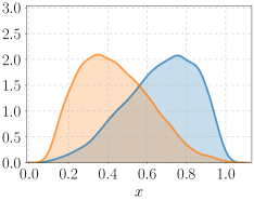
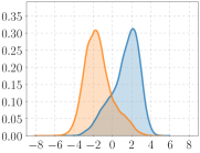
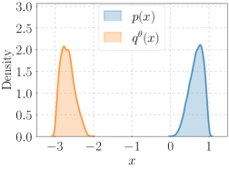
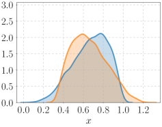
Alignment in distributions implies alignment in supports. However, when there are additional objectives/constraints to satisfy, the minimizer for a distribution alignment objective does not necessarily minimize a support alignment objective. Example in Figure 1 demonstrates the qualitative distinction between two minimizers when distribution alignment is not achievable. The distribution alignment objective prefers to keep supports unaligned even if support alignment is achievable. Recent works (Zhao et al., 2019; Li et al., 2020; Tan et al., 2020; Wu et al., 2019b; Tachet des Combes et al., 2020) have demonstrated that a shift in label distributions between source and target leads to a characterizable performance drop when the representations are forced into a distribution alignment. The error bound in Johansson et al. (2019) suggests aligning the supports of representations instead.

In this paper, we focus on distribution support as the key characteristic to align. We introduce a support divergence to measure the support mismatch and algorithms to optimize such alignment. We also position our approach in the spectrum of other alignment methods. Our contributions are as follows (all proofs can be found in Appendix A):

  1. 1.

    In Section 2.1, we measure the differences between supports of distributions. Building on the Hausdorff distance, we introduce a novel support divergence better suited for optimization, which we refer to as symmetric support difference (SSD) divergence.

  2. 2.

    In Section 2.2, we identify an important property of the discriminator trained for Jensen–Shannon divergence: support differences in the original space of interest are “preserved” as support differences in the one-dimensional discriminator output space.

  3. 3.

    In Section 3, we present our practical algorithm for support alignment, Adversarial Support Alignment (ASA). Essentially, based on the analysis presented in Section 2.2, our solution is to align supports in the discriminator 1D space, which is computationally efficient.

  4. 4.

    In Section 4, we place different notions of alignment – distribution alignment, relaxed distribution alignment and support alignment – within a coherent spectrum from the point of view of optimal transport, characterizing their relationships, both theoretically in terms of their objectives and practically in terms of their algorithms.

  5. 5.

    In Section 5, we demonstrate the effectiveness of support alignment in practice for domain adaptation setting. Compared to other alignment-based baselines, our proposed method is more robust against shifts in label distributions.
Refer to caption
(a) Initialization
𝒟W(p,qθ)=11.12subscript𝒟𝑊𝑝superscript𝑞𝜃11.12\mathcal{D}_{W}(p,q^{\theta})=11.12
𝒟(p,qθ)=14.9subscript𝒟𝑝superscript𝑞𝜃14.9\mathcal{D}_{\triangle}(p,q^{\theta})=14.9
Refer to caption
(b) Distribution alignment
𝒟W(p,qθ)=2103subscript𝒟𝑊𝑝superscript𝑞𝜃2superscript103\mathcal{D}_{W}(p,q^{\theta})=2\cdot 10^{-3}
𝒟(p,qθ)=6104subscript𝒟𝑝superscript𝑞𝜃6superscript104\mathcal{D}_{\triangle}(p,q^{\theta})=6\cdot 10^{-4}
Refer to caption
(c) Support alignment
𝒟W(p,qθ)=5102subscript𝒟𝑊𝑝superscript𝑞𝜃5superscript102\mathcal{D}_{W}(p,q^{\theta})=5\cdot 10^{-2}
𝒟(p,qθ)<1106subscript𝒟𝑝superscript𝑞𝜃1superscript106\mathcal{D}_{\triangle}(p,q^{\theta})<1\cdot 10^{-6}
Figure 1: Illustration of differences between the final configurations of distribution alignment and support alignment procedures. p(x)𝑝𝑥p(x) is a fixed Beta distribution p(x)=Beta(x| 4,2)𝑝𝑥Betaconditional𝑥42p(x)=\operatorname{Beta}(x\,|\,4,2) with support [0,1]01[0,1]; qθ(x)superscript𝑞𝜃𝑥q^{\theta}(x) is a “shifted” Beta distribution qθ(x)=Beta(xθ| 2,4)superscript𝑞𝜃𝑥Beta𝑥conditional𝜃24q^{\theta}(x)=\operatorname{Beta}(x-\theta\,|\,2,4) parameterized by θ𝜃\theta with support [θ,θ+1]𝜃𝜃1[\theta,\theta+1]. Panel (a) shows the initial configuration with θinit=3subscript𝜃init3\theta_{\text{init}}=-3. Panel (b) shows the result by distribution alignment. Panel (c) shows the result by support alignment. We report Wasserstein distance 𝒟W(p,qθ)subscript𝒟𝑊𝑝superscript𝑞𝜃\mathcal{D}_{W}(p,q^{\theta}) (7) and SSD divergence 𝒟(p,qθ)subscript𝒟𝑝superscript𝑞𝜃\mathcal{D}_{\triangle}(p,q^{\theta}) (1).

2 SSD divergence and support alignment

Notation. We consider an Euclidean space 𝒳=n𝒳superscript𝑛\mathcal{X}=\mathbb{R}^{n} equipped with Borel sigma algebra \mathcal{B} and a metric d:𝒳×𝒳:𝑑𝒳𝒳d:\mathcal{X}\times\mathcal{X}\to\mathbb{R} (e.g. Euclidean distance). Let 𝒫𝒫\mathcal{P} be the set of probability measures on (𝒳,)𝒳(\mathcal{X},\mathcal{B}). For p𝒫𝑝𝒫p\in\mathcal{P}, the support of p𝑝p is denoted by supp(p)supp𝑝\operatorname*{supp}(p) and is defined as the smallest closed set X𝒳𝑋𝒳X\subseteq\mathcal{X} such that p(X)=1𝑝𝑋1p(X)=1. fpsubscript𝑓𝑝f_{\sharp}p denotes the pushforward measure of p𝑝p induced by a measurable mapping f𝑓f. With a slight abuse of notation, we use p(x)𝑝𝑥p(x) and [fp](t)delimited-[]subscript𝑓𝑝𝑡[f_{\sharp}p](t) to denote the densities of measures p𝑝p and fpsubscript𝑓𝑝f_{\sharp}p evaluated at x𝑥x and t𝑡t respectively, implicitly assuming that the measures are absolutely continuous. The distance between a point x𝒳𝑥𝒳x\in\mathcal{X} and a subset Y𝒳𝑌𝒳Y\subseteq\mathcal{X} is defined as d(x,Y)=infyYd(x,y)𝑑𝑥𝑌subscriptinfimum𝑦𝑌𝑑𝑥𝑦d(x,Y)=\inf_{y\in Y}d(x,y). The symmetric difference of two sets A𝐴A and B𝐵B is defined as AB=(AB)(BA)𝐴𝐵𝐴𝐵𝐵𝐴A\,\triangle\,B=\left(A\setminus B\right)\cup\left(B\setminus A\right).

2.1 Difference between supports

To align the supports of distributions, we first need to evaluate how different they are. Similar to distribution divergences like Jensen–Shannon divergence, we introduce a notion of support divergence. A support divergence222It is not technically a divergence on the space of distributions, since 𝒟S(p,q)=0subscript𝒟𝑆𝑝𝑞0\mathcal{D}_{S}(p,q)=0 does not imply p=q𝑝𝑞p=q. between two distributions in 𝒫𝒫\mathcal{P} is a function 𝒟S(,):𝒫×𝒫:subscript𝒟𝑆𝒫𝒫\mathcal{D}_{S}(\cdot,\cdot):\mathcal{P}\times\mathcal{P}\rightarrow\mathbb{R} satisfying: 1) 𝒟S(p,q)0subscript𝒟𝑆𝑝𝑞0\mathcal{D}_{S}(p,q)\geq 0 for all p,q𝒫𝑝𝑞𝒫p,q\in\mathcal{P}; 2) 𝒟S(p,q)=0subscript𝒟𝑆𝑝𝑞0\mathcal{D}_{S}(p,q)=0 iff supp(p)=supp(q)supp𝑝supp𝑞\operatorname{supp}(p)=\operatorname{supp}(q).

While a distribution divergence is sensitive to both density and support differences, a support divergence only needs to detect mismatches in supports, which are subsets of the metric space 𝒳𝒳\mathcal{X}. An example of a distance between subsets of a metric space is the Hausdorff distance: dH(X,Y)=max{supxXd(x,Y),supyYd(y,X)}subscript𝑑𝐻𝑋𝑌subscriptsupremum𝑥𝑋𝑑𝑥𝑌subscriptsupremum𝑦𝑌𝑑𝑦𝑋d_{H}(X,Y)=\max\{\sup_{x\in X}d(x,Y),\sup_{y\in Y}d(y,X)\}. Since it depends only on the greatest distance between a point and a set, minimizing this objective for alignment only provides signal to a single point. To make the optimization less sparse, we consider all points that violate the support alignment criterion and introduce symmetric support difference (SSD) divergence:

𝒟(p,q)=𝔼xp[d(x,supp(q))]+𝔼xq[d(x,supp(p))].subscript𝒟𝑝𝑞subscript𝔼similar-to𝑥𝑝delimited-[]𝑑𝑥supp𝑞subscript𝔼similar-to𝑥𝑞delimited-[]𝑑𝑥supp𝑝\mathcal{D}_{\triangle}(p,q)=\mathbb{E}_{x\sim p}\left[d(x,\operatorname{supp}(q))\right]+\mathbb{E}_{x\sim q}\left[d(x,\operatorname{supp}(p))\right]. (1)
Proposition 2.1.

SSD divergence 𝒟(p,q)subscript𝒟𝑝𝑞\mathcal{D}_{\triangle}(p,q) is a support divergence.

We note that our proposed SSD divergence is closely related to Chamfer distance/divergence (CD) (Fan et al., 2017; Nguyen et al., 2021) and Relaxed Word Mover’s Distance (RWMD) (Kusner et al., 2015). While both CD and RWMD are stated for discrete points (see Section 6 for further comments), SSD divergence is a general difference measure between arbitrary (discrete or continuous) distributions. This distinction, albeit small, is important in our theoretical analysis (Sections 2.2, 4.1).

2.2 Support alignment in one-dimensional space

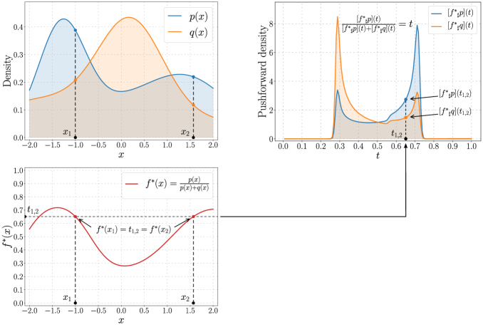
Goodfellow et al. (2014) showed that the log-loss discriminator f:𝒳[0,1]:𝑓𝒳01f:\mathcal{X}\to[0,1], trained to distinguish samples from distributions p𝑝p and q𝑞q (supf𝔼xp[logf(x)]+𝔼xq[log(1f(x))]subscriptsupremum𝑓subscript𝔼similar-to𝑥𝑝delimited-[]𝑓𝑥subscript𝔼similar-to𝑥𝑞delimited-[]1𝑓𝑥\sup_{f}\ \mathbb{E}_{x\sim p}\left[\log f(x)\right]+\mathbb{E}_{x\sim q}\left[\log(1-f(x))\right]) can be used to estimate the Jensen–Shannon divergence between p𝑝p and q𝑞q. The closed form maximizer fsuperscript𝑓f^{*} is

f(x)=p(x)p(x)+q(x),xsupp(p)supp(q).formulae-sequencesuperscript𝑓𝑥𝑝𝑥𝑝𝑥𝑞𝑥for-all𝑥supp𝑝supp𝑞f^{*}(x)=\frac{p(x)}{p(x)+q(x)},\qquad\forall x\in\operatorname{supp}(p)\cup\operatorname{supp}(q). (2)

Note that for a point xsupp(p)supp(q)𝑥supp𝑝supp𝑞x\notin\operatorname*{supp}(p)\cup\operatorname*{supp}(q) the value of f(x)superscript𝑓𝑥f^{*}(x) can be set to an arbitrary value in [0,1]01[0,1], since the log-loss does not depend on f(x)𝑓𝑥f(x) for such x𝑥x. The form of the optimal discriminator (2) gives rise to our main theorem below, which characterizes the ability of the log-loss discriminator to identify support misalignment.

Theorem 2.1.

Suppose distributions p𝑝p and q𝑞q have densities satisfying

1C<p(x)<C,xsupp(p);1C<q(x)<C,xsupp(q).formulae-sequence1𝐶𝑝𝑥𝐶formulae-sequencefor-all𝑥supp𝑝1𝐶𝑞𝑥𝐶for-all𝑥supp𝑞\frac{1}{C}<p(x)<C,\quad\forall\,x\in\operatorname*{supp}(p);\qquad\frac{1}{C}<q(x)<C,\quad\forall\,x\in\operatorname*{supp}(q). (3)

Let fsuperscript𝑓f^{*} be the optimal discriminator (2). Then, 𝒟(p,q)=0subscript𝒟𝑝𝑞0\mathcal{D}_{\triangle}(p,q)=0 if and only if 𝒟(fp,fq)=0subscript𝒟subscriptsuperscript𝑓𝑝subscriptsuperscript𝑓𝑞0\mathcal{D}_{\triangle}({f^{*}}_{\sharp}p,{f^{*}}_{\sharp}q)=0.

The idea of the proof is to show that the extreme values (00 and 111) of f(x)superscript𝑓𝑥f^{*}(x) can only be attained in xsupp(p)supp(q)𝑥supp𝑝supp𝑞x\in\operatorname*{supp}(p)\triangle\operatorname*{supp}(q). Assumption (3) guarantees that f(x)superscript𝑓𝑥f^{*}(x) cannot approach neither 00 nor 111 in the intersection of the supports supp(p)supp(q)supp𝑝supp𝑞\operatorname*{supp}(p)\cap\operatorname*{supp}(q), i.e. the values {f(x)|xsupp(p)supp(q)}conditional-setsuperscript𝑓𝑥𝑥supp𝑝supp𝑞\{f^{*}(x)\,|\,x\in\operatorname*{supp}(p)\cap\operatorname*{supp}(q)\} are separated from the extreme values 00 and 111.

We conclude this section with two technical remarks on Theorem 2.1.

Remark 2.1.1.

The result of Theorem 2.1 does not necessarily hold for other types of discriminators. For instance, the dual Wasserstein discriminator (Arjovsky et al., 2017; Gulrajani et al., 2017) does not always highlight the support difference in the original space as a support difference in the discriminator output space. This observation is formaly stated in the following proposition.

Proposition 2.2.

Let fWsubscriptsuperscript𝑓𝑊f^{\star}_{W} be the maximizer of supf:L(f)1𝔼xp[f(x)]𝔼xq[f(x)]subscriptsupremum:𝑓L𝑓1subscript𝔼similar-to𝑥𝑝delimited-[]𝑓𝑥subscript𝔼similar-to𝑥𝑞delimited-[]𝑓𝑥\sup_{f:\operatorname{L}(f)\leq 1}\mathbb{E}_{x\sim p}[f(x)]-\mathbb{E}_{x\sim q}[f(x)], where L()L\operatorname{L}(\cdot) is the Lipschitz constant. There exist p𝑝p and q𝑞q with supp(p)supp(q)supp𝑝supp𝑞\operatorname{supp}(p)\neq\operatorname{supp}(q) but supp(fWp)=supp(fWq)suppsubscriptsubscriptsuperscript𝑓𝑊𝑝suppsubscriptsubscriptsuperscript𝑓𝑊𝑞\operatorname{supp}({f^{\star}_{W}}_{\sharp}p)=\operatorname{supp}({f^{\star}_{W}}_{\sharp}q).

Remark 2.1.2.

In practice the discriminator is typically parameterized as f(x)=σ(g(x))𝑓𝑥𝜎𝑔𝑥f(x)=\sigma(g(x)), where g:𝒳:𝑔𝒳g:\mathcal{X}\to\mathbb{R} is realized by a deep neural network and σ(x)=(1+ex)1𝜎𝑥superscript1superscript𝑒𝑥1\sigma(x)=(1+e^{-x})^{-1} is the sigmoid function. The optimization problem for g𝑔g is

infg𝔼xp[log(1+eg(x))]+𝔼xq[log(1+eg(x))],subscriptinfimum𝑔subscript𝔼similar-to𝑥𝑝delimited-[]1superscript𝑒𝑔𝑥subscript𝔼similar-to𝑥𝑞delimited-[]1superscript𝑒𝑔𝑥\inf_{g}\ \mathbb{E}_{x\sim p}\left[\log(1+e^{-g(x)})\right]+\mathbb{E}_{x\sim q}\left[\log(1+e^{g(x)})\right], (4)

and the optimal solution is g(x)=logp(x)logq(x)superscript𝑔𝑥𝑝𝑥𝑞𝑥g^{*}(x)=\log p(x)-\log q(x). Naturally the result of Theorem 2.1 holds for gsuperscript𝑔g^{*}, since g(x)=σ1(f(x))superscript𝑔𝑥superscript𝜎1superscript𝑓𝑥g^{*}(x)=\sigma^{-1}(f^{*}(x)) and σ𝜎\sigma is a bijective mapping from {,}\mathbb{R}\cup\{-\infty,\infty\} to [0,1]01[0,1].

3 Adversarial support alignment

We consider distributions p𝑝p and q𝑞q parameterized by θ𝜃\theta: pθ,qθsuperscript𝑝𝜃superscript𝑞𝜃p^{\theta},q^{\theta}. The log-loss discriminator g𝑔g optimized for (4) is parameterized by ψ𝜓\psi: gψsuperscript𝑔𝜓g^{\psi}. Our analysis in Section 2.2 already suggests an algorithm. Namely, we can optimize θ𝜃\theta by minimizing 𝒟(gψpθ,gψqθ)subscript𝒟subscriptsuperscript𝑔𝜓superscript𝑝𝜃subscriptsuperscript𝑔𝜓superscript𝑞𝜃\mathcal{D}_{\triangle}({g^{\psi}}_{\sharp}p^{\theta},{g^{\psi}}_{\sharp}q^{\theta}) while optimizing ψ𝜓\psi by (4). This adversarial game is analogous to the setup of the existing distribution alignment algorithms333Following existing adversarial distribution alignment methods, e.g. (Goodfellow et al., 2014), we use single update of ψ𝜓\psi per 111 update of θ𝜃\theta. While theoretical analysis for both distribution alignment and support alignment (ours) assume optimal discriminators, training with single update of ψ𝜓\psi is computationally cheap and effective..

In practice, rather than having direct access to pθ,qθsuperscript𝑝𝜃superscript𝑞𝜃p^{\theta},q^{\theta}, which is unavailable, we are often given i.i.d. samples {xip}i=1N,{xiq}i=1Msuperscriptsubscriptsuperscriptsubscript𝑥𝑖𝑝𝑖1𝑁superscriptsubscriptsuperscriptsubscript𝑥𝑖𝑞𝑖1𝑀\{x_{i}^{p}\}_{i=1}^{N},\{x_{i}^{q}\}_{i=1}^{M}. They form discrete distributions p^θ(x)=1Ni=1Nδ(xxip),q^θ(x)=1Mi=1Mδ(xxiq)formulae-sequencesuperscript^𝑝𝜃𝑥1𝑁superscriptsubscript𝑖1𝑁𝛿𝑥superscriptsubscript𝑥𝑖𝑝superscript^𝑞𝜃𝑥1𝑀superscriptsubscript𝑖1𝑀𝛿𝑥superscriptsubscript𝑥𝑖𝑞\hat{p}^{\theta}(x)=\frac{1}{N}\sum_{i=1}^{N}\delta(x-x_{i}^{p}),\hat{q}^{\theta}(x)=\frac{1}{M}\sum_{i=1}^{M}\delta(x-x_{i}^{q}), and [gψp^θ](t)=1Ni=1Nδ(tgψ(xip)),[gψq^θ](t)=1Mi=1Mδ(tgψ(xiq))formulae-sequencedelimited-[]subscriptsuperscript𝑔𝜓superscript^𝑝𝜃𝑡1𝑁superscriptsubscript𝑖1𝑁𝛿𝑡superscript𝑔𝜓superscriptsubscript𝑥𝑖𝑝delimited-[]subscriptsuperscript𝑔𝜓superscript^𝑞𝜃𝑡1𝑀superscriptsubscript𝑖1𝑀𝛿𝑡superscript𝑔𝜓superscriptsubscript𝑥𝑖𝑞[{g^{\psi}}_{\sharp}\hat{p}^{\theta}](t)=\frac{1}{N}\sum_{i=1}^{N}\delta(t-g^{\psi}(x_{i}^{p})),[{g^{\psi}}_{\sharp}\hat{q}^{\theta}](t)=\frac{1}{M}\sum_{i=1}^{M}\delta(t-g^{\psi}(x_{i}^{q})). Since gψp^θsubscriptsuperscript𝑔𝜓superscript^𝑝𝜃{g^{\psi}}_{\sharp}\hat{p}^{\theta} and gψq^θsubscriptsuperscript𝑔𝜓superscript^𝑞𝜃{g^{\psi}}_{\sharp}\hat{q}^{\theta} are discrete distributions, they have supports {gψ(xip)}i=1Nsuperscriptsubscriptsuperscript𝑔𝜓superscriptsubscript𝑥𝑖𝑝𝑖1𝑁\{g^{\psi}(x_{i}^{p})\}_{i=1}^{N} and {gψ(xiq)}i=1Msuperscriptsubscriptsuperscript𝑔𝜓superscriptsubscript𝑥𝑖𝑞𝑖1𝑀\{g^{\psi}(x_{i}^{q})\}_{i=1}^{M} respectively. SSD divergence between discrete distributions gψp^θsubscriptsuperscript𝑔𝜓superscript^𝑝𝜃{g^{\psi}}_{\sharp}\hat{p}^{\theta} and gψq^θsubscriptsuperscript𝑔𝜓superscript^𝑞𝜃{g^{\psi}}_{\sharp}\hat{q}^{\theta} is

𝒟(gψp^θ,gψq^θ)=1Ni=1Nd(gψ(xip),{gψ(xjq)}j=1M)+1Mi=1Md(gψ(xiq),{gψ(xjp)}j=1N).subscript𝒟subscriptsuperscript𝑔𝜓superscript^𝑝𝜃subscriptsuperscript𝑔𝜓superscript^𝑞𝜃1𝑁superscriptsubscript𝑖1𝑁𝑑superscript𝑔𝜓superscriptsubscript𝑥𝑖𝑝superscriptsubscriptsuperscript𝑔𝜓superscriptsubscript𝑥𝑗𝑞𝑗1𝑀1𝑀superscriptsubscript𝑖1𝑀𝑑superscript𝑔𝜓superscriptsubscript𝑥𝑖𝑞superscriptsubscriptsuperscript𝑔𝜓superscriptsubscript𝑥𝑗𝑝𝑗1𝑁\mathcal{D}_{\triangle}({g^{\psi}}_{\sharp}\hat{p}^{\theta},{g^{\psi}}_{\sharp}\hat{q}^{\theta})=\frac{1}{N}\sum_{i=1}^{N}d\left(g^{\psi}(x_{i}^{p}),\{g^{\psi}(x_{j}^{q})\}_{j=1}^{M}\right)+\frac{1}{M}\sum_{i=1}^{M}d\left(g^{\psi}(x_{i}^{q}),\{g^{\psi}(x_{j}^{p})\}_{j=1}^{N}\right). (5)

Effect of mini-batch training. When training on large datasets, we need to rely on stochastic optimization with mini-batches. We denote the mini-batches (of same size, as in common practice) from pθsuperscript𝑝𝜃p^{\theta} and qθsuperscript𝑞𝜃q^{\theta} as xp={xip}i=1msuperscript𝑥𝑝superscriptsubscriptsuperscriptsubscript𝑥𝑖𝑝𝑖1𝑚x^{p}=\{x_{i}^{p}\}_{i=1}^{m} and xq={xiq}i=1msuperscript𝑥𝑞superscriptsubscriptsuperscriptsubscript𝑥𝑖𝑞𝑖1𝑚x^{q}=\{x_{i}^{q}\}_{i=1}^{m} respectively. By minimizing 𝒟(gψ(xp),gψ(xq))subscript𝒟superscript𝑔𝜓superscript𝑥𝑝superscript𝑔𝜓superscript𝑥𝑞\mathcal{D}_{\triangle}(g^{\psi}(x^{p}),g^{\psi}(x^{q})), we only consider the mini-batch support distance rather than the population support distance (5). We observe that in practice the described algorithm brings the distributions to a state closer to distribution alignment rather than support alignment (see Appendix D.5 for details). The problem is in the typically small batch size. The algorithm actually aims to enforce support alignment for all possible pairs of mini-batches, which is a much stricter constraint than population support alignment.

To address the issue mentioned above, without working with a much larger batch size, we create two “history buffers”: hpsuperscript𝑝h^{p}, storing the previous 1D discriminator outputs of (at most) n𝑛n samples from pθsuperscript𝑝𝜃p^{\theta}, and a similar buffer hqsuperscript𝑞h^{q} for qθsuperscript𝑞𝜃q^{\theta}. Specifically, h={gψold,i(xold,i)}i=1nsuperscriptsubscriptsuperscript𝑔subscript𝜓old𝑖subscript𝑥old𝑖𝑖1𝑛h=\{g^{\psi_{\text{old},i}}(x_{\text{old},i})\}_{i=1}^{n} stores the values of the previous n𝑛n samples xold,isubscript𝑥old𝑖x_{\text{old},i} mapped by their corresponding past “versions” of the discriminator gψold,isuperscript𝑔subscript𝜓old𝑖g^{\psi_{\text{old},i}}. We minimize 𝒟(vp,vq)subscript𝒟superscript𝑣𝑝superscript𝑣𝑞\mathcal{D}_{\triangle}(v^{p},v^{q}), where vp=concat(hp,gψ(xp))superscript𝑣𝑝concatsuperscript𝑝superscript𝑔𝜓superscript𝑥𝑝v^{p}=\operatorname{concat}(h^{p},g^{\psi}(x^{p})), vq=concat(hq,gψ(xq))superscript𝑣𝑞concatsuperscript𝑞superscript𝑔𝜓superscript𝑥𝑞v^{q}=\operatorname{concat}(h^{q},g^{\psi}(x^{q})):

𝒟(vp,vq)=1n+m(i=1n+md(vip,vq)+j=1n+md(vjq,vp)).subscript𝒟superscript𝑣𝑝superscript𝑣𝑞1𝑛𝑚superscriptsubscript𝑖1𝑛𝑚𝑑subscriptsuperscript𝑣𝑝𝑖superscript𝑣𝑞superscriptsubscript𝑗1𝑛𝑚𝑑subscriptsuperscript𝑣𝑞𝑗superscript𝑣𝑝\mathcal{D}_{\triangle}(v^{p},v^{q})=\frac{1}{n+m}\left(\sum_{i=1}^{n+m}d(v^{p}_{i},v^{q})+\sum_{j=1}^{n+m}d(v^{q}_{j},v^{p})\right). (6)

Note that 𝒟(,)subscript𝒟\mathcal{D}_{\triangle}(\cdot,\cdot) between two sets of 1D samples can be efficiently calculated since d(vip,vq)𝑑subscriptsuperscript𝑣𝑝𝑖superscript𝑣𝑞d(v^{p}_{i},v^{q}) and d(vjq,vp)𝑑subscriptsuperscript𝑣𝑞𝑗superscript𝑣𝑝d(v^{q}_{j},v^{p}) are simply 1-nearest neighbor distances in 1D. Moreover the history buffers store only the scalar values from the previous batches. These values are only considered in nearest neighbor assignment but do not directly provide gradient signal for optimization. Thus, the computation overhead of including a long history buffer is very light. We present our full algorithm, Adversarial Support Alignment (ASA), in Algorithm 1.

Algorithm 1 Our proposed ASA algorithm. n𝑛n (maximum history buffer size), we use n=1000𝑛1000n=1000.
1:for number of training steps do
2:     Sample mini-batches {xip}i=1mpθsimilar-tosuperscriptsubscriptsubscriptsuperscript𝑥𝑝𝑖𝑖1𝑚superscript𝑝𝜃\{x^{p}_{i}\}_{i=1}^{m}\sim p^{\theta}{xiq}i=1mqθsimilar-tosuperscriptsubscriptsubscriptsuperscript𝑥𝑞𝑖𝑖1𝑚superscript𝑞𝜃\{x^{q}_{i}\}_{i=1}^{m}\sim q^{\theta}.
3:     Perform optimization step on ψ𝜓\psi using stochastic gradient     ψ(1mi=1m[log(1+exp(gψ(xip)))+log(1+exp(gψ(xiq)))])subscript𝜓1𝑚superscriptsubscript𝑖1𝑚delimited-[]1superscript𝑔𝜓subscriptsuperscript𝑥𝑝𝑖1superscript𝑔𝜓subscriptsuperscript𝑥𝑞𝑖\nabla_{\psi}\left(\frac{1}{m}\sum\limits_{i=1}^{m}\Big{[}\log(1+\exp(-g^{\psi}(x^{p}_{i})))+\log(1+\exp(g^{\psi}(x^{q}_{i})))\Big{]}\right).
4:     vpconcat(hp,{gψ(xip)}i=1m)superscript𝑣𝑝concatsuperscript𝑝superscriptsubscriptsuperscript𝑔𝜓subscriptsuperscript𝑥𝑝𝑖𝑖1𝑚v^{p}\leftarrow\operatorname{concat}(h^{p},\{g^{\psi}(x^{p}_{i})\}_{i=1}^{m}),   vqconcat(hq,{gψ(xiq)}i=1m)superscript𝑣𝑞concatsuperscript𝑞superscriptsubscriptsuperscript𝑔𝜓subscriptsuperscript𝑥𝑞𝑖𝑖1𝑚v^{q}\leftarrow\operatorname{concat}(h^{q},\{g^{\psi}(x^{q}_{i})\}_{i=1}^{m}).
5:     πpqiargminjd(vip,vjq)superscriptsubscript𝜋𝑝𝑞𝑖subscriptargmin𝑗𝑑subscriptsuperscript𝑣𝑝𝑖subscriptsuperscript𝑣𝑞𝑗\pi_{p\rightarrow q}^{i}\leftarrow\operatorname*{arg\,min}_{j}d(v^{p}_{i},v^{q}_{j}),   πqpjargminid(vip,vjq)superscriptsubscript𝜋𝑞𝑝𝑗subscriptargmin𝑖𝑑subscriptsuperscript𝑣𝑝𝑖subscriptsuperscript𝑣𝑞𝑗\pi_{q\rightarrow p}^{j}\leftarrow\operatorname*{arg\,min}_{i}d(v^{p}_{i},v^{q}_{j}).
6:     Perform optimization step on θ𝜃\theta using stochastic gradient     θ(1n+mi=1n+m[d(vip,vπpqiq)+d(viq,vπqpip)])subscript𝜃1𝑛𝑚superscriptsubscript𝑖1𝑛𝑚delimited-[]𝑑subscriptsuperscript𝑣𝑝𝑖subscriptsuperscript𝑣𝑞superscriptsubscript𝜋𝑝𝑞𝑖𝑑subscriptsuperscript𝑣𝑞𝑖subscriptsuperscript𝑣𝑝superscriptsubscript𝜋𝑞𝑝𝑖\nabla_{\theta}\left(\frac{1}{n+m}\sum\limits_{i=1}^{n+m}\Big{[}d(v^{p}_{i},v^{q}_{\pi_{p\rightarrow q}^{i}})+d(v^{q}_{i},v^{p}_{\pi_{q\rightarrow p}^{i}})\Big{]}\right).
7:     UpdateHistory(hp,{gψ(xip)}i=1m)superscript𝑝superscriptsubscriptsuperscript𝑔𝜓subscriptsuperscript𝑥𝑝𝑖𝑖1𝑚(h^{p},\{g^{\psi}(x^{p}_{i})\}_{i=1}^{m}),   UpdateHistory(hq,{gψ(xiq)}i=1m)superscript𝑞superscriptsubscriptsuperscript𝑔𝜓subscriptsuperscript𝑥𝑞𝑖𝑖1𝑚(h^{q},\{g^{\psi}(x^{q}_{i})\}_{i=1}^{m}).
8:end for

4 Spectrum of notions of alignment

In this section, we take a closer look into our work and different existing notions of alignment that have been proposed in the literature, especially their formulations from the optimal transport perspective. We show that our proposed support alignment framework is a limit of existing notions of alignment, both in terms of theory and algorithm, by increasing transportation assignment tolerance.

4.1 Theoretical connections

Distribution alignment. Wasserstein distance is a commonly used objective for distribution alignment. In our analysis, we focus on the Wasserstein-1 distance:

𝒟W(p,q)=infγΓ(p,q)𝔼(x,y)γ[d(x,y)],subscript𝒟𝑊𝑝𝑞subscriptinfimum𝛾Γ𝑝𝑞subscript𝔼similar-to𝑥𝑦𝛾delimited-[]𝑑𝑥𝑦\mathcal{D}_{W}(p,q)=\inf_{\gamma\in\Gamma(p,q)}\mathbb{E}_{(x,y)\sim\gamma}[d(x,y)], (7)

where Γ(p,q)Γ𝑝𝑞\Gamma(p,q) is the set of all measures on 𝒳×𝒳𝒳𝒳\mathcal{X}\times\mathcal{X} with marginals of p𝑝p and q𝑞q, respectively. The value of 𝒟W(p,q)subscript𝒟𝑊𝑝𝑞\mathcal{D}_{W}(p,q) is the minimal transportation cost for transporting probability mass from p𝑝p to q𝑞q. The transportation cost is zero if and only if p=q𝑝𝑞p=q, meaning the distributions are aligned.

Relaxed distribution alignment. Wu et al. (2019b) proposed a modified Wasserstein distance to achieve asymmetrically-relaxed distribution alignment, namely β𝛽\beta-admissible Wasserstein distance:

𝒟Wβ(p,q)=infγΓβ(p,q)𝔼(x,y)γ[d(x,y)],superscriptsubscript𝒟𝑊𝛽𝑝𝑞subscriptinfimum𝛾subscriptΓ𝛽𝑝𝑞subscript𝔼similar-to𝑥𝑦𝛾delimited-[]𝑑𝑥𝑦\mathcal{D}_{W}^{\beta}(p,q)=\inf_{\gamma\in\Gamma_{\beta}(p,q)}\mathbb{E}_{(x,y)\sim\gamma}[d(x,y)], (8)

where Γβ(p,q)subscriptΓ𝛽𝑝𝑞\Gamma_{\beta}(p,q) is the set of all measures γ𝛾\gamma on 𝒳×𝒳𝒳𝒳\mathcal{X}\times\mathcal{X} such that γ(x,y)𝑑y=p(x),x𝛾𝑥𝑦differential-d𝑦𝑝𝑥for-all𝑥\int\gamma(x,y)dy=p(x),\forall x and γ(x,y)𝑑x(1+β)q(y),y𝛾𝑥𝑦differential-d𝑥1𝛽𝑞𝑦for-all𝑦\int\gamma(x,y)dx\leq(1+\beta)q(y),\forall y. With the relaxed marginal constraints, one could choose a transportation plan γ𝛾\gamma which transports probability mass from p𝑝p to a modified distribution qsuperscript𝑞q^{\prime} rather than the original distribution q𝑞q as long as qsuperscript𝑞q^{\prime} satisfies the constraint q(x)(1+β)q(x),xsuperscript𝑞𝑥1𝛽𝑞𝑥for-all𝑥q^{\prime}(x)\leq(1+\beta)q(x),\forall x. Therefore, 𝒟Wβ(p,q)superscriptsubscript𝒟𝑊𝛽𝑝𝑞\mathcal{D}_{W}^{\beta}(p,q) is zero if and only if p(x)(1+β)q(x),x𝑝𝑥1𝛽𝑞𝑥for-all𝑥p(x)\leq(1+\beta)q(x),\forall x. In (Wu et al., 2019b), β𝛽\beta is normally set to a positive finite number to achieve the asymmetric-relaxation of distribution alignment, and it is shown that 𝒟W0(p,q)=𝒟W(p,q)superscriptsubscript𝒟𝑊0𝑝𝑞subscript𝒟𝑊𝑝𝑞\mathcal{D}_{W}^{0}(p,q)=\mathcal{D}_{W}(p,q). We can extend 𝒟Wβ(p,q)superscriptsubscript𝒟𝑊𝛽𝑝𝑞\mathcal{D}_{W}^{\beta}(p,q) to a symmetric version, which we term β1,β2subscript𝛽1subscript𝛽2\beta_{1},\beta_{2}-admissible Wasserstein distance:

𝒟Wβ1,β2(p,q)=𝒟Wβ1(p,q)+𝒟Wβ2(q,p).superscriptsubscript𝒟𝑊subscript𝛽1subscript𝛽2𝑝𝑞superscriptsubscript𝒟𝑊subscript𝛽1𝑝𝑞superscriptsubscript𝒟𝑊subscript𝛽2𝑞𝑝\mathcal{D}_{W}^{\beta_{1},\beta_{2}}(p,q)=\mathcal{D}_{W}^{\beta_{1}}(p,q)+\mathcal{D}_{W}^{\beta_{2}}(q,p). (9)

The aforementioned property of β𝛽\beta-admissible Wasserstein distance implies that 𝒟Wβ1,β2(p,q)=0superscriptsubscript𝒟𝑊subscript𝛽1subscript𝛽2𝑝𝑞0\mathcal{D}_{W}^{\beta_{1},\beta_{2}}(p,q)=0 if and only if p(x)(1+β1)q(x),x𝑝𝑥1subscript𝛽1𝑞𝑥for-all𝑥p(x)\leq(1+\beta_{1})q(x),\forall x and q(x)(1+β2)p(x),x𝑞𝑥1subscript𝛽2𝑝𝑥for-all𝑥q(x)\leq(1+\beta_{2})p(x),\forall x, in which case we call p𝑝p and q𝑞q(β1,β2)subscript𝛽1subscript𝛽2(\beta_{1},\beta_{2})-aligned”, with β1subscript𝛽1\beta_{1} and β2subscript𝛽2\beta_{2} controlling the transportation assignment tolerances.

Support alignment. The term 𝔼p[d(x,supp(q))]subscript𝔼𝑝delimited-[]𝑑𝑥supp𝑞\mathbb{E}_{p}[d(x,\operatorname*{supp}(q))] in (1) represents the average distance from samples in p𝑝p to the support of q𝑞q. From the optimal transport perspective, this value is the minimal transportation cost of transporting the probability mass of p𝑝p into the support of q𝑞q. We show that SSD divergence can be considered as a transportation cost in the limit of infinite assignment tolerance.

Proposition 4.1.

𝒟W,(p,q)limβ1,β2𝒟Wβ1,β2(p,q)=𝒟(p,q)superscriptsubscript𝒟𝑊𝑝𝑞subscriptsubscript𝛽1subscript𝛽2superscriptsubscript𝒟𝑊subscript𝛽1subscript𝛽2𝑝𝑞subscript𝒟𝑝𝑞\mathcal{D}_{W}^{\infty,\infty}(p,q)\coloneqq\lim_{\beta_{1},\beta_{2}\to\infty}\mathcal{D}_{W}^{\beta_{1},\beta_{2}}(p,q)=\mathcal{D}_{\triangle}(p,q).

We now have completed the spectrum of alignment objectives defined within the optimal transport framework. The following proposition establishes the relationship within the spectrum.

Proposition 4.2.

Let p𝑝p and q𝑞q be two distributions in 𝒫𝒫\mathcal{P}. Then,

  1. 1.

    𝒟W(p,q)=0subscript𝒟𝑊𝑝𝑞0\mathcal{D}_{W}(p,q)=0 implies 𝒟Wβ1,β2(p,q)=0superscriptsubscript𝒟𝑊subscript𝛽1subscript𝛽2𝑝𝑞0\mathcal{D}_{W}^{\beta_{1},\beta_{2}}(p,q)=0 for all finite β1,β2>0subscript𝛽1subscript𝛽20\beta_{1},\beta_{2}>0.

  2. 2.

    𝒟Wβ1,β2(p,q)=0superscriptsubscript𝒟𝑊subscript𝛽1subscript𝛽2𝑝𝑞0\mathcal{D}_{W}^{\beta_{1},\beta_{2}}(p,q)=0 for some finite β1,β2>0subscript𝛽1subscript𝛽20\beta_{1},\beta_{2}>0 implies 𝒟(p,q)=0subscript𝒟𝑝𝑞0\mathcal{D}_{\triangle}(p,q)=0.

  3. 3.

    The converse of statements 1 and 2 are false.

In addition to the result presented in Theorem 2.1, we can show that the log-loss discriminator can also “preserve” the existing notions of alignment.

Proposition 4.3.

Let fsuperscript𝑓f^{*} be the optimal discriminator (2) for given distributions p𝑝p and q𝑞q. Then,

1. 𝒟W(p,q)=0subscript𝒟𝑊𝑝𝑞0\mathcal{D}_{W}(p,q)=0iff 𝒟W(fp,fq)=0subscript𝒟𝑊subscriptsuperscript𝑓𝑝subscriptsuperscript𝑓𝑞0\mathcal{D}_{W}({f^{*}}_{\sharp}p,{f^{*}}_{\sharp}q)=0;     2. 𝒟Wβ1,β2(p,q)=0subscriptsuperscript𝒟subscript𝛽1subscript𝛽2𝑊𝑝𝑞0\mathcal{D}^{\beta_{1},\beta_{2}}_{W}(p,q)=0iff 𝒟Wβ1,β2(fp,fq)=0subscriptsuperscript𝒟subscript𝛽1subscript𝛽2𝑊subscriptsuperscript𝑓𝑝subscriptsuperscript𝑓𝑞0\mathcal{D}^{\beta_{1},\beta_{2}}_{W}({f^{*}}_{\sharp}p,{f^{*}}_{\sharp}q)=0.

4.2 Algorithmic connections

The result of Proposition 4.3 suggests methods similar to our ASA algorithm presented in Section 3 can achieve different notions of alignment by minimizing objectives discussed in Section 4.1 between the 1D pushforward distributions. We consider the setup used in Section 3 but without history buffers to simplify the analysis, as their usage is orthogonal to our discussion in this section.

Recall that we work with a mini-batch setting, where {xip}i=1msuperscriptsubscriptsubscriptsuperscript𝑥𝑝𝑖𝑖1𝑚\{x^{p}_{i}\}_{i=1}^{m} and {xiq}i=1msuperscriptsubscriptsubscriptsuperscript𝑥𝑞𝑖𝑖1𝑚\{x^{q}_{i}\}_{i=1}^{m} are sampled from p𝑝p and q𝑞q respectively, and g𝑔g is the adversarial log-loss discriminator. We denote the corresponding 1D outputs from the log-loss discriminator by op={oip}i=1m={g(xip)}i=1msuperscript𝑜𝑝superscriptsubscriptsubscriptsuperscript𝑜𝑝𝑖𝑖1𝑚superscriptsubscript𝑔subscriptsuperscript𝑥𝑝𝑖𝑖1𝑚o^{p}=\{o^{p}_{i}\}_{i=1}^{m}=\{g(x^{p}_{i})\}_{i=1}^{m} and oqsuperscript𝑜𝑞o^{q} (defined similarly).

Distribution alignment. We adapt (7) for {oip}i=1msuperscriptsubscriptsubscriptsuperscript𝑜𝑝𝑖𝑖1𝑚\{o^{p}_{i}\}_{i=1}^{m} and {oiq}i=1msuperscriptsubscriptsubscriptsuperscript𝑜𝑞𝑖𝑖1𝑚\{o^{q}_{i}\}_{i=1}^{m}:

𝒟W(op,oq)=infγΓ(op,oq)1mi=1mj=1mγijd(oip,ojq),subscript𝒟𝑊superscript𝑜𝑝superscript𝑜𝑞subscriptinfimum𝛾Γsuperscript𝑜𝑝superscript𝑜𝑞1𝑚superscriptsubscript𝑖1𝑚superscriptsubscript𝑗1𝑚subscript𝛾𝑖𝑗𝑑subscriptsuperscript𝑜𝑝𝑖subscriptsuperscript𝑜𝑞𝑗\mathcal{D}_{W}(o^{p},o^{q})=\inf_{\gamma\in\Gamma(o^{p},o^{q})}\frac{1}{m}\sum_{i=1}^{m}\sum_{j=1}^{m}\gamma_{ij}d(o^{p}_{i},o^{q}_{j}), (10)

where Γ(op,oq)Γsuperscript𝑜𝑝superscript𝑜𝑞\Gamma(o^{p},o^{q}) is the set of m×m𝑚𝑚m\times m doubly stochastic matrices. Since opsuperscript𝑜𝑝o^{p} and oqsuperscript𝑜𝑞o^{q} are sets of 1D samples with the same size, it can be shown (Rabin et al., 2011) that the optimal γsuperscript𝛾\gamma^{*} corresponds to an assignment πsuperscript𝜋\pi^{*}, which pairs points in the sorting order and can be computed efficiently by sorting both sets opsuperscript𝑜𝑝o^{p} and oqsuperscript𝑜𝑞o^{q}. The transportation cost is zero if and only if there exists an invertible 111-to-111 assignment πsuperscript𝜋\pi^{*} such that oip=oπ(i)qsubscriptsuperscript𝑜𝑝𝑖subscriptsuperscript𝑜𝑞superscript𝜋𝑖o^{p}_{i}=o^{q}_{\pi^{*}(i)}. GAN training algorithms proposed in (Deshpande et al., 2018; 2019) utilize the above sorting procedure to estimate the maximum sliced Wasserstein distance.

Relaxed distribution alignment. Similarly, we can adapt (8):

𝒟Wβ(op,oq)=infγΓβ(op,oq)1mi=1mj=1mγijd(oip,ojq),superscriptsubscript𝒟𝑊𝛽superscript𝑜𝑝superscript𝑜𝑞subscriptinfimum𝛾subscriptΓ𝛽superscript𝑜𝑝superscript𝑜𝑞1𝑚superscriptsubscript𝑖1𝑚superscriptsubscript𝑗1𝑚subscript𝛾𝑖𝑗𝑑subscriptsuperscript𝑜𝑝𝑖subscriptsuperscript𝑜𝑞𝑗\mathcal{D}_{W}^{\beta}(o^{p},o^{q})=\inf_{\gamma\in\Gamma_{\beta}(o^{p},o^{q})}\frac{1}{m}\sum_{i=1}^{m}\sum_{j=1}^{m}\gamma_{ij}d(o^{p}_{i},o^{q}_{j}), (11)

where Γβ(op,oq)subscriptΓ𝛽superscript𝑜𝑝superscript𝑜𝑞\Gamma_{\beta}(o^{p},o^{q}) is the set of m×m𝑚𝑚m\times m matrices with non-negative real entries, such that j=1mγij=1,isuperscriptsubscript𝑗1𝑚subscript𝛾𝑖𝑗1for-all𝑖\sum_{j=1}^{m}\gamma_{ij}=1,\forall i and i=1mγij1+β,jsuperscriptsubscript𝑖1𝑚subscript𝛾𝑖𝑗1𝛽for-all𝑗\sum_{i=1}^{m}\gamma_{ij}\leq 1+\beta,\forall j. The optimization goal in (11) is to find a “soft-assignment” γ𝛾\gamma which describes the transportation of probability mass from points oipsubscriptsuperscript𝑜𝑝𝑖o^{p}_{i} in opsuperscript𝑜𝑝o^{p} to points oiqsubscriptsuperscript𝑜𝑞𝑖o^{q}_{i} in oqsuperscript𝑜𝑞o^{q}. The parameter β𝛽\beta controls the set of admissible assignments ΓβsubscriptΓ𝛽\Gamma_{\beta}, which is similar to its role discussed in Section 4.1: with transportation assignment tolerance β𝛽\beta, the total mass of points in opsuperscript𝑜𝑝o^{p} transported to each of the points oiqsubscriptsuperscript𝑜𝑞𝑖o^{q}_{i} cannot exceed 1+β1𝛽1+\beta. We refer to such assignments as (β+1)𝛽1(\beta+1)-to-111 assignment. The transportation cost is zero if and only if there exists such an assignment between opsuperscript𝑜𝑝o^{p} and oqsuperscript𝑜𝑞o^{q}.

It can be shown (see Appendix C) that for integer value of β𝛽\beta, the set of minimizers of (11) must contain a “hard-assignment” transportation plan, which assigns each point oipsubscriptsuperscript𝑜𝑝𝑖o^{p}_{i} to exactly one point ojqsubscriptsuperscript𝑜𝑞𝑗o^{q}_{j}. Then (1+β)1𝛽(1+\beta) gives the upper bound on the number of points oipsubscriptsuperscript𝑜𝑝𝑖o^{p}_{i} that can be transported to given point ojqsubscriptsuperscript𝑜𝑞𝑗o^{q}_{j}. This hard assignment problem can be solved quasi-linearly with worst case time complexity 𝒪((β+1)m2)𝒪𝛽1superscript𝑚2\mathcal{O}\left((\beta+1)m^{2}\right) (Bonneel & Coeurjolly, 2019), which, combined with Proposition 4.3, can lead to new algorithms for relaxed distribution alignment besides those proposed in Wu et al. (2019b).

Support alignment. When β=𝛽\beta=\infty, the sum i=1mγijsuperscriptsubscript𝑖1𝑚subscript𝛾𝑖𝑗\sum_{i=1}^{m}\gamma_{ij} is unconstrained for all j𝑗j, and each point oipsubscriptsuperscript𝑜𝑝𝑖o^{p}_{i} can be assigned to any of the points ojqsubscriptsuperscript𝑜𝑞𝑗o^{q}_{j}. The optimal solution is simply 1-nearest neighbor assignment, or to follow the above terminology, \infty-to-111 assignment.

5 Experiments

Refer to caption
(a) No DA (avg acc: 63%percent6363\%)
𝒟W(pZθ,qZθ)=0.78subscript𝒟𝑊subscriptsuperscript𝑝𝜃𝑍subscriptsuperscript𝑞𝜃𝑍0.78\mathcal{D}_{W}(p^{\theta}_{Z},q^{\theta}_{Z})=0.78
𝒟(pZθ,qZθ)=0.10subscript𝒟subscriptsuperscript𝑝𝜃𝑍subscriptsuperscript𝑞𝜃𝑍0.10\mathcal{D}_{\triangle}(p^{\theta}_{Z},q^{\theta}_{Z})=0.10
Refer to caption
(b) DANN (avg acc: 75%percent7575\%)
𝒟W(pZθ,qZθ)=0.07subscript𝒟𝑊subscriptsuperscript𝑝𝜃𝑍subscriptsuperscript𝑞𝜃𝑍0.07\mathcal{D}_{W}(p^{\theta}_{Z},q^{\theta}_{Z})=0.07
𝒟(pZθ,qZθ)=0.02subscript𝒟subscriptsuperscript𝑝𝜃𝑍subscriptsuperscript𝑞𝜃𝑍0.02\mathcal{D}_{\triangle}(p^{\theta}_{Z},q^{\theta}_{Z})=0.02
Refer to caption
(c) ASA-abs (avg acc: 94%percent9494\%)
𝒟W(pZθ,qZθ)=0.59subscript𝒟𝑊subscriptsuperscript𝑝𝜃𝑍subscriptsuperscript𝑞𝜃𝑍0.59\mathcal{D}_{W}(p^{\theta}_{Z},q^{\theta}_{Z})=0.59
𝒟(pZθ,qZθ)=0.03subscript𝒟subscriptsuperscript𝑝𝜃𝑍subscriptsuperscript𝑞𝜃𝑍0.03\mathcal{D}_{\triangle}(p^{\theta}_{Z},q^{\theta}_{Z})=0.03
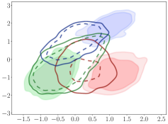
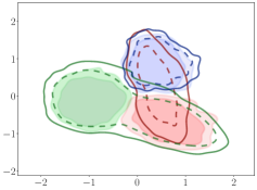
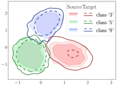
Figure 2: Visualization of learned 2D embeddings on 3-class USPS\toMNIST with label distribution shift. In source domain, all classes have equal probability 1313\frac{1}{3}. The target probabilities of classes ‘3’, ‘5’, ‘9’ are [23%,65%,12%]percent23percent65percent12[23\%,65\%,12\%]. Each panel shows 2 level sets (outer one approximates the support) of the kernel density estimates of embeddings in source (filled regions) and target domains (solid/dashed lines). We report the average class accuracy of the target domain, 𝒟Wsubscript𝒟𝑊\mathcal{D}_{W} and 𝒟subscript𝒟\mathcal{D}_{\triangle} between embeddings.

Problem setting. We evaluate our proposed ASA method in the setting of unsupervised domain adaptation (UDA). The goal of UDA algorithms is to train and “adapt” a classification model M:𝒳𝒴:𝑀𝒳𝒴M:\mathcal{X}\to\mathcal{Y} from source domain distribution pX,Ysubscript𝑝𝑋𝑌p_{X,Y} to target domain distribution qX,Ysubscript𝑞𝑋𝑌q_{X,Y} given the access to a labeled source dataset {xip,yip}i=1NppX,Ysimilar-tosuperscriptsubscriptsubscriptsuperscript𝑥𝑝𝑖subscriptsuperscript𝑦𝑝𝑖𝑖1superscript𝑁𝑝subscript𝑝𝑋𝑌\{x^{p}_{i},y^{p}_{i}\}_{i=1}^{N^{p}}\sim p_{X,Y} and an unlabeled target dataset {xiq}i=1NqqXsimilar-tosuperscriptsubscriptsubscriptsuperscript𝑥𝑞𝑖𝑖1superscript𝑁𝑞subscript𝑞𝑋\{x^{q}_{i}\}_{i=1}^{N^{q}}\sim q_{X}.

A common approach for UDA is to represent M𝑀M as CϕFθsuperscript𝐶italic-ϕsuperscript𝐹𝜃C^{\phi}\circ F^{\theta}: a classifier Cϕ:𝒵𝒴:superscript𝐶italic-ϕ𝒵𝒴C^{\phi}:\mathcal{Z}\to\mathcal{Y} and a feature extractor Fθ:𝒳𝒵:superscript𝐹𝜃𝒳𝒵F^{\theta}:\mathcal{X}\to\mathcal{Z}, and train Cϕsuperscript𝐶italic-ϕC^{\phi} and Fθsuperscript𝐹𝜃F^{\theta} by minimizing: 1) classification loss clssubscriptcls\ell_{\text{cls}} on source examples; 2) alignment loss 𝒟alignsubscript𝒟align\mathcal{D}_{\text{align}} measuring discrepancy between pZθ=FθpXsubscriptsuperscript𝑝𝜃𝑍subscriptsuperscript𝐹𝜃subscript𝑝𝑋p^{\theta}_{Z}={F^{\theta}}_{\sharp}p_{X} and qZθ=FθqXsubscriptsuperscript𝑞𝜃𝑍subscriptsuperscript𝐹𝜃subscript𝑞𝑋q^{\theta}_{Z}={F^{\theta}}_{\sharp}q_{X}:

minϕ,θ1Npi=1Npcls(Cϕ(Fθ(xip)),yip)+λ𝒟align({Fθ(xip)}i=1Np,{Fθ(xiq)}i=1Nq),subscriptitalic-ϕ𝜃1superscript𝑁𝑝superscriptsubscript𝑖1superscript𝑁𝑝subscriptclssuperscript𝐶italic-ϕsuperscript𝐹𝜃subscriptsuperscript𝑥𝑝𝑖subscriptsuperscript𝑦𝑝𝑖𝜆subscript𝒟alignsuperscriptsubscriptsuperscript𝐹𝜃subscriptsuperscript𝑥𝑝𝑖𝑖1superscript𝑁𝑝superscriptsubscriptsuperscript𝐹𝜃subscriptsuperscript𝑥𝑞𝑖𝑖1superscript𝑁𝑞\min_{\phi,\theta}\;\;\frac{1}{N^{p}}\sum\limits_{i=1}^{N^{p}}\ell_{\text{cls}}(C^{\phi}(F^{\theta}(x^{p}_{i})),y^{p}_{i})+\lambda\cdot\mathcal{D}_{\text{align}}\left(\{F^{\theta}(x^{p}_{i})\}_{i=1}^{N^{p}},\{F^{\theta}(x^{q}_{i})\}_{i=1}^{N^{q}}\right), (12)

In practice 𝒟alignsubscript𝒟align\mathcal{D}_{\text{align}} is an estimate of a divergence measure via an adversarial discriminator gψsuperscript𝑔𝜓g^{\psi}. Choices of 𝒟alignsubscript𝒟align\mathcal{D}_{\text{align}} include f-divergences (Ganin et al., 2016; Nowozin et al., 2016) and Wasserstein distance (Arjovsky et al., 2017) to enforce distribution alignment and versions of re-weighted/relaxed distribution divergences (Wu et al., 2019b; Tachet des Combes et al., 2020) to enforce relaxed distribution alignment. For support alignment, we apply the proposed ASA method as the alignment subroutine in (12) with log-loss discriminator gψsuperscript𝑔𝜓g^{\psi} (4) and 𝒟alignsubscript𝒟align\mathcal{D}_{\text{align}} computed as (6).

Task specifications. We consider 3 UDA tasks: USPS\toMNIST, STL\toCIFAR, and VisDA-2017, and 2 versions of ASA: ASA-sq, ASA-abs corresponding to squared and absolute distances respectively for d(,)𝑑d(\cdot,\cdot) in (6). We compare ASA with: No DA (no domain adaptation), DANN (Ganin et al., 2016) (distribution alignment with JS divergence), VADA (Shu et al., 2018) (distribution alignment with virtual adversarial training), IWDAN, IWCDAN (Tachet des Combes et al., 2020) (relaxed distribution alignment via importance weighting) sDANN-β𝛽\bm{\beta} (Wu et al., 2019b) (relaxed/β𝛽\beta-admissible JS divergence via re-weighting). Please refer to Appendix D for full experimental details.

To evaluate the robustness of the methods, we simulate label distribution shift by subsampling source and target dataset, so that source has balanced label distribution and target label distribution follows the power law qY(y)σ(y)αproportional-tosubscript𝑞𝑌𝑦𝜎superscript𝑦𝛼q_{Y}(y)\varpropto\sigma(y)^{-\alpha}, where σ𝜎\sigma is a random permutation of class labels {1,,K}1𝐾\{1,\ldots,K\} and α𝛼\alpha controls the severity of the shift (α=0𝛼0\alpha=0 means balanced label distribution). For each task, we generate 5 random permutations σ𝜎\sigma for 444 different shift levels α{0,1,1.5,2}𝛼011.52\alpha\in\{0,1,1.5,2\}. Essentially we transform each (source, target) dataset pair to 5×4=2054205\times 4=20 tasks of different difficulty levels, since classes are not equally difficult and different permutations can give them different weights.

Evaluation metrics. We choose the average (per-)class accuracy and minimum (per-)class accuracy on the target test set as evaluation metrics. Under the average class accuracy metric, all classes are treated as equally important (despite the unequal representation during training for α>0𝛼0\alpha>0), and the minimum class accuracy focuses on model’s worst within-class performance. In order to account for the variability of task difficulties across random permutations of target labels, we report robust statistics, median and a 25-75 percentile interval, across 5 runs.

Illustrative example. First we consider a simplified setting to intuitively understand and directly analyze the behavior of our proposed support alignment method in domain adaptation under label distribution shift. We consider a 3-class USPS\toMNIST problem by selecting a subset of examples corresponding to digits ‘3’, ‘5’, and ‘9’, and use a feature extractor network with 2D output space. We introduce label distribution shift as described above with α=1.5𝛼1.5\alpha=1.5, i.e. the probabilities of classes in the target domain are 12%percent1212\%, 23%percent2323\%, and 65%percent6565\%. We compare No DA, DANN, ASA-abs by their average target classification accuracy, Wasserstein distance 𝒟W(pZθ,qZθ)subscript𝒟𝑊subscriptsuperscript𝑝𝜃𝑍subscriptsuperscript𝑞𝜃𝑍\mathcal{D}_{W}(p^{\theta}_{Z},q^{\theta}_{Z}) and SSD divergence 𝒟(pZθ,qZθ)subscript𝒟subscriptsuperscript𝑝𝜃𝑍subscriptsuperscript𝑞𝜃𝑍\mathcal{D}_{\triangle}(p^{\theta}_{Z},q^{\theta}_{Z}) between the learned embeddings of source and target domain. We apply a global affine transformation to each embedding space in order to have comparable distances between different spaces: we center the embeddings so that their average is 0 and re-scale them so that their average norm is 1. The results are shown in Figure 2 and Table D.5. Compared to No DA, both DANN and ASA achieve support alignment. DANN enforces distribution alignment, and thus places some target embeddings into regions corresponding to the wrong class. In comparison, ASA does not enforce distribution alignment and maintains good class correspondence across the source and target embeddings.

Table 1: Average and minimum class accuracy (%percent\%) on USPS\rightarrowMNIST with different levels of shifts in label distributions (higher α𝛼\alpha implies more severe imbalance). We report median (the main number), and 25 (subscript) and 75 (superscript) percentiles across 5 runs.
α=0.0𝛼0.0\alpha=0.0 α=1.0𝛼1.0\alpha=1.0 α=1.5𝛼1.5\alpha=1.5 α=2.0𝛼2.0\alpha=2.0
Algorithm average min average min average min average min
No DA 71.970.472.9superscriptsubscript71.970.472.971.9_{~{}70.4}^{~{}72.9} 20.317.622.9superscriptsubscript20.317.622.920.3_{~{}17.6}^{~{}22.9} 72.972.074.7superscriptsubscript72.972.074.772.9_{~{}72.0}^{~{}74.7} 25.818.331.8superscriptsubscript25.818.331.825.8_{~{}18.3}^{~{}31.8} 71.371.272.5superscriptsubscript71.371.272.571.3_{~{}71.2}^{~{}72.5} 27.524.237.3superscriptsubscript27.524.237.327.5_{~{}24.2}^{~{}37.3} 71.370.673.0superscriptsubscript71.370.673.071.3_{~{}70.6}^{~{}73.0} 16.610.826.8superscriptsubscript16.610.826.816.6_{~{}10.8}^{~{}26.8}
DANN 97.897.697.8superscriptsubscript97.897.697.897.8_{~{}97.6}^{~{}97.8} 96.095.896.1superscriptsubscript96.095.896.196.0_{~{}95.8}^{~{}96.1} 83.576.784.6superscriptsubscript83.576.784.683.5_{~{}76.7}^{~{}84.6} 25.108.436.9superscriptsubscript25.108.436.925.1_{~{}08.4}^{~{}36.9} 70.063.971.2superscriptsubscript70.063.971.270.0_{~{}63.9}^{~{}71.2} 01.101.001.5superscriptsubscript01.101.001.501.1_{~{}01.0}^{~{}01.5} 57.852.060.4superscriptsubscript57.852.060.457.8_{~{}52.0}^{~{}60.4} 00.900.501.6superscriptsubscript00.900.501.600.9_{~{}00.5}^{~{}01.6}
VADA 98.097.998.0superscriptsubscript98.097.998.0\textbf{98.0}_{~{}97.9}^{~{}98.0} 96.295.996.3superscriptsubscript96.295.996.396.2_{~{}95.9}^{~{}96.3} 88.288.189.9superscriptsubscript88.288.189.988.2_{~{}88.1}^{~{}89.9} 48.947.850.0superscriptsubscript48.947.850.048.9_{~{}47.8}^{~{}50.0} 78.270.783.1superscriptsubscript78.270.783.178.2_{~{}70.7}^{~{}83.1} 06.602.423.5superscriptsubscript06.602.423.506.6_{~{}02.4}^{~{}23.5} 61.956.365.4superscriptsubscript61.956.365.461.9_{~{}56.3}^{~{}65.4} 01.400.801.5superscriptsubscript01.400.801.501.4_{~{}00.8}^{~{}01.5}
IWDAN 97.597.497.5superscriptsubscript97.597.497.597.5_{~{}97.4}^{~{}97.5} 95.795.795.9superscriptsubscript95.795.795.995.7_{~{}95.7}^{~{}95.9} 95.792.695.8superscriptsubscript95.792.695.895.7_{~{}92.6}^{~{}95.8} 81.367.182.3superscriptsubscript81.367.182.381.3_{~{}67.1}^{~{}82.3} 86.580.287.8superscriptsubscript86.580.287.886.5_{~{}80.2}^{~{}87.8} 15.204.255.0superscriptsubscript15.204.255.015.2_{~{}04.2}^{~{}55.0} 74.470.078.6superscriptsubscript74.470.078.674.4_{~{}70.0}^{~{}78.6} 07.306.322.4superscriptsubscript07.306.322.407.3_{~{}06.3}^{~{}22.4}
IWCDAN 98.097.998.1superscriptsubscript98.097.998.1\textbf{98.0}_{~{}97.9}^{~{}98.1} 96.696.496.9superscriptsubscript96.696.496.9\textbf{96.6}_{~{}96.4}^{~{}96.9} 96.793.397.5superscriptsubscript96.793.397.5\textbf{96.7}_{~{}93.3}^{~{}97.5} 85.165.393.9superscriptsubscript85.165.393.985.1_{~{}65.3}^{~{}93.9} 91.390.593.8superscriptsubscript91.390.593.891.3_{~{}90.5}^{~{}93.8} 66.564.174.5superscriptsubscript66.564.174.566.5_{~{}64.1}^{~{}74.5} 77.577.382.3superscriptsubscript77.577.382.377.5_{~{}77.3}^{~{}82.3} 22.202.745.4superscriptsubscript22.202.745.422.2_{~{}02.7}^{~{}45.4}
sDANN-4 87.487.295.7superscriptsubscript87.487.295.787.4_{~{}87.2}^{~{}95.7} 05.605.690.0superscriptsubscript05.605.690.005.6_{~{}05.6}^{~{}90.0} 94.994.794.9superscriptsubscript94.994.794.994.9_{~{}94.7}^{~{}94.9} 85.784.487.7superscriptsubscript85.784.487.7\textbf{85.7}_{~{}84.4}^{~{}87.7} 86.885.589.1superscriptsubscript86.885.589.186.8_{~{}85.5}^{~{}89.1} 21.615.450.3superscriptsubscript21.615.450.321.6_{~{}15.4}^{~{}50.3} 81.581.383.1superscriptsubscript81.581.383.181.5_{~{}81.3}^{~{}83.1} 39.337.956.2superscriptsubscript39.337.956.239.3_{~{}37.9}^{~{}56.2}
ASA-sq 93.793.393.9superscriptsubscript93.793.393.993.7_{~{}93.3}^{~{}93.9} 89.288.489.4superscriptsubscript89.288.489.489.2_{~{}88.4}^{~{}89.4} 92.391.593.6superscriptsubscript92.391.593.692.3_{~{}91.5}^{~{}93.6} 83.580.888.7superscriptsubscript83.580.888.783.5_{~{}80.8}^{~{}88.7} 90.989.692.1superscriptsubscript90.989.692.190.9_{~{}89.6}^{~{}92.1} 69.966.682.0superscriptsubscript69.966.682.069.9_{~{}66.6}^{~{}82.0} 87.285.889.3superscriptsubscript87.285.889.387.2_{~{}85.8}^{~{}89.3} 62.546.469.3superscriptsubscript62.546.469.362.5_{~{}46.4}^{~{}69.3}
ASA-abs 94.193.894.5superscriptsubscript94.193.894.594.1_{~{}93.8}^{~{}94.5} 88.987.091.2superscriptsubscript88.987.091.288.9_{~{}87.0}^{~{}91.2} 92.889.393.2superscriptsubscript92.889.393.292.8_{~{}89.3}^{~{}93.2} 78.965.182.9superscriptsubscript78.965.182.978.9_{~{}65.1}^{~{}82.9} 92.590.992.9superscriptsubscript92.590.992.9\textbf{92.5}_{~{}90.9}^{~{}92.9} 82.474.585.4superscriptsubscript82.474.585.4\textbf{82.4}_{~{}74.5}^{~{}85.4} 90.489.290.7superscriptsubscript90.489.290.7\textbf{90.4}_{~{}89.2}^{~{}90.7} 68.467.573.0superscriptsubscript68.467.573.0\textbf{68.4}_{~{}67.5}^{~{}73.0}
Table 2: Results on STL\rightarrowCIFAR. Same setup and reporting metrics as Table 1.
α=0.0𝛼0.0\alpha=0.0 α=1.0𝛼1.0\alpha=1.0 α=1.5𝛼1.5\alpha=1.5 α=2.0𝛼2.0\alpha=2.0
Algorithm average min average min average min average min
No DA 69.969.870.0superscriptsubscript69.969.870.069.9_{~{}69.8}^{~{}70.0} 49.845.350.6superscriptsubscript49.845.350.649.8_{~{}45.3}^{~{}50.6} 68.868.369.3superscriptsubscript68.868.369.368.8_{~{}68.3}^{~{}69.3} 47.245.348.2superscriptsubscript47.245.348.247.2_{~{}45.3}^{~{}48.2} 66.866.467.2superscriptsubscript66.866.467.266.8_{~{}66.4}^{~{}67.2} 46.045.847.0superscriptsubscript46.045.847.046.0_{~{}45.8}^{~{}47.0} 65.864.866.7superscriptsubscript65.864.866.765.8_{~{}64.8}^{~{}66.7} 43.741.644.6superscriptsubscript43.741.644.643.7_{~{}41.6}^{~{}44.6}
DANN 75.374.975.4superscriptsubscript75.374.975.475.3_{~{}74.9}^{~{}75.4} 54.654.256.6superscriptsubscript54.654.256.654.6_{~{}54.2}^{~{}56.6} 69.968.670.1superscriptsubscript69.968.670.169.9_{~{}68.6}^{~{}70.1} 44.840.745.1superscriptsubscript44.840.745.144.8_{~{}40.7}^{~{}45.1} 64.963.767.1superscriptsubscript64.963.767.164.9_{~{}63.7}^{~{}67.1} 34.933.936.8superscriptsubscript34.933.936.834.9_{~{}33.9}^{~{}36.8} 63.357.464.8superscriptsubscript63.357.464.863.3_{~{}57.4}^{~{}64.8} 27.021.228.5superscriptsubscript27.021.228.527.0_{~{}21.2}^{~{}28.5}
VADA 76.776.676.7superscriptsubscript76.776.676.7\textbf{76.7}_{~{}76.6}^{~{}76.7} 56.953.558.3superscriptsubscript56.953.558.3\textbf{56.9}_{~{}53.5}^{~{}58.3} 70.670.071.0superscriptsubscript70.670.071.070.6_{~{}70.0}^{~{}71.0} 47.744.048.8superscriptsubscript47.744.048.847.7_{~{}44.0}^{~{}48.8} 66.165.466.5superscriptsubscript66.165.466.566.1_{~{}65.4}^{~{}66.5} 35.733.339.3superscriptsubscript35.733.339.335.7_{~{}33.3}^{~{}39.3} 63.260.264.7superscriptsubscript63.260.264.763.2_{~{}60.2}^{~{}64.7} 25.525.228.0superscriptsubscript25.525.228.025.5_{~{}25.2}^{~{}28.0}
IWDAN 69.969.970.7superscriptsubscript69.969.970.769.9_{~{}69.9}^{~{}70.7} 50.547.950.6superscriptsubscript50.547.950.650.5_{~{}47.9}^{~{}50.6} 68.768.669.1superscriptsubscript68.768.669.168.7_{~{}68.6}^{~{}69.1} 45.844.850.5superscriptsubscript45.844.850.545.8_{~{}44.8}^{~{}50.5} 67.165.967.3superscriptsubscript67.165.967.367.1_{~{}65.9}^{~{}67.3} 44.740.444.8superscriptsubscript44.740.444.844.7_{~{}40.4}^{~{}44.8} 64.463.664.9superscriptsubscript64.463.664.964.4_{~{}63.6}^{~{}64.9} 36.834.537.9superscriptsubscript36.834.537.936.8_{~{}34.5}^{~{}37.9}
IWCDAN 70.170.170.2superscriptsubscript70.170.170.270.1_{~{}70.1}^{~{}70.2} 47.842.449.3superscriptsubscript47.842.449.347.8_{~{}42.4}^{~{}49.3} 69.469.169.4superscriptsubscript69.469.169.469.4_{~{}69.1}^{~{}69.4} 47.146.351.3superscriptsubscript47.146.351.347.1_{~{}46.3}^{~{}51.3} 66.165.067.2superscriptsubscript66.165.067.266.1_{~{}65.0}^{~{}67.2} 39.937.740.8superscriptsubscript39.937.740.839.9_{~{}37.7}^{~{}40.8} 64.563.965.1superscriptsubscript64.563.965.164.5_{~{}63.9}^{~{}65.1} 37.035.540.2superscriptsubscript37.035.540.237.0_{~{}35.5}^{~{}40.2}
sDANN-4 71.871.772.1superscriptsubscript71.871.772.171.8_{~{}71.7}^{~{}72.1} 52.152.152.8superscriptsubscript52.152.152.852.1_{~{}52.1}^{~{}52.8} 71.170.471.7superscriptsubscript71.170.471.7\textbf{71.1}_{~{}70.4}^{~{}71.7} 49.948.151.8superscriptsubscript49.948.151.849.9_{~{}48.1}^{~{}51.8} 69.468.770.0superscriptsubscript69.468.770.069.4_{~{}68.7}^{~{}70.0} 48.643.549.0superscriptsubscript48.643.549.0\textbf{48.6}_{~{}43.5}^{~{}49.0} 66.466.267.9superscriptsubscript66.466.267.966.4_{~{}66.2}^{~{}67.9} 39.033.647.1superscriptsubscript39.033.647.139.0_{~{}33.6}^{~{}47.1}
ASA-sq 71.771.771.9superscriptsubscript71.771.771.971.7_{~{}71.7}^{~{}71.9} 52.946.753.4superscriptsubscript52.946.753.452.9_{~{}46.7}^{~{}53.4} 70.770.471.0superscriptsubscript70.770.471.070.7_{~{}70.4}^{~{}71.0} 51.646.852.7superscriptsubscript51.646.852.7\textbf{51.6}_{~{}46.8}^{~{}52.7} 69.269.269.3superscriptsubscript69.269.269.369.2_{~{}69.2}^{~{}69.3} 45.643.352.0superscriptsubscript45.643.352.045.6_{~{}43.3}^{~{}52.0} 68.167.268.2superscriptsubscript68.167.268.2\textbf{68.1}_{~{}67.2}^{~{}68.2} 44.739.845.9superscriptsubscript44.739.845.9\textbf{44.7}_{~{}39.8}^{~{}45.9}
ASA-abs 71.671.271.7superscriptsubscript71.671.271.771.6_{~{}71.2}^{~{}71.7} 49.048.453.5superscriptsubscript49.048.453.549.0_{~{}48.4}^{~{}53.5} 70.970.871.0superscriptsubscript70.970.871.070.9_{~{}70.8}^{~{}71.0} 49.247.350.0superscriptsubscript49.247.350.049.2_{~{}47.3}^{~{}50.0} 69.669.669.9superscriptsubscript69.669.669.9\textbf{69.6}_{~{}69.6}^{~{}69.9} 43.242.149.5superscriptsubscript43.242.149.543.2_{~{}42.1}^{~{}49.5} 67.866.668.2superscriptsubscript67.866.668.267.8_{~{}66.6}^{~{}68.2} 40.935.449.0superscriptsubscript40.935.449.040.9_{~{}35.4}^{~{}49.0}
Table 3: Results on VisDA17. Same setup and reporting metrics as Table 1.
α=0.0𝛼0.0\alpha=0.0 α=1.0𝛼1.0\alpha=1.0 α=1.5𝛼1.5\alpha=1.5 α=2.0𝛼2.0\alpha=2.0
Algorithm average min average min average min average min
No DA 49.549.450.5superscriptsubscript49.549.450.549.5_{~{}49.4}^{~{}50.5} 22.222.224.6superscriptsubscript22.222.224.622.2_{~{}22.2}^{~{}24.6} 50.249.250.8superscriptsubscript50.249.250.850.2_{~{}49.2}^{~{}50.8} 21.220.721.3superscriptsubscript21.220.721.321.2_{~{}20.7}^{~{}21.3} 47.146.647.6superscriptsubscript47.146.647.647.1_{~{}46.6}^{~{}47.6} 18.618.622.2superscriptsubscript18.618.622.218.6_{~{}18.6}^{~{}22.2} 45.345.246.5superscriptsubscript45.345.246.545.3_{~{}45.2}^{~{}46.5} 19.514.419.8superscriptsubscript19.514.419.819.5_{~{}14.4}^{~{}19.8}
DANN 75.474.476.2superscriptsubscript75.474.476.2\textbf{75.4}_{~{}74.4}^{~{}76.2} 36.735.640.9superscriptsubscript36.735.640.936.7_{~{}35.6}^{~{}40.9} 64.162.865.3superscriptsubscript64.162.865.364.1_{~{}62.8}^{~{}65.3} 25.024.829.3superscriptsubscript25.024.829.325.0_{~{}24.8}^{~{}29.3} 52.151.452.3superscriptsubscript52.151.452.352.1_{~{}51.4}^{~{}52.3} 11.511.412.4superscriptsubscript11.511.412.411.5_{~{}11.4}^{~{}12.4} 43.139.144.3superscriptsubscript43.139.144.343.1_{~{}39.1}^{~{}44.3} 03.603.614.3superscriptsubscript03.603.614.303.6_{~{}03.6}^{~{}14.3}
VADA 75.374.876.0superscriptsubscript75.374.876.075.3_{~{}74.8}^{~{}76.0} 40.539.741.8superscriptsubscript40.539.741.840.5_{~{}39.7}^{~{}41.8} 64.661.265.1superscriptsubscript64.661.265.164.6_{~{}61.2}^{~{}65.1} 22.821.728.2superscriptsubscript22.821.728.222.8_{~{}21.7}^{~{}28.2} 53.051.654.2superscriptsubscript53.051.654.253.0_{~{}51.6}^{~{}54.2} 14.813.721.7superscriptsubscript14.813.721.714.8_{~{}13.7}^{~{}21.7} 43.940.944.7superscriptsubscript43.940.944.743.9_{~{}40.9}^{~{}44.7} 08.505.011.1superscriptsubscript08.505.011.108.5_{~{}05.0}^{~{}11.1}
IWDAN 73.272.973.3superscriptsubscript73.272.973.373.2_{~{}72.9}^{~{}73.3} 31.722.834.8superscriptsubscript31.722.834.831.7_{~{}22.8}^{~{}34.8} 64.461.164.6superscriptsubscript64.461.164.664.4_{~{}61.1}^{~{}64.6} 12.105.024.7superscriptsubscript12.105.024.712.1_{~{}05.0}^{~{}24.7} 51.351.056.6superscriptsubscript51.351.056.651.3_{~{}51.0}^{~{}56.6} 04.602.110.4superscriptsubscript04.602.110.404.6_{~{}02.1}^{~{}10.4} 45.141.748.0superscriptsubscript45.141.748.045.1_{~{}41.7}^{~{}48.0} 04.601.213.6superscriptsubscript04.601.213.604.6_{~{}01.2}^{~{}13.6}
IWCDAN 71.670.675.2superscriptsubscript71.670.675.271.6_{~{}70.6}^{~{}75.2} 27.622.828.0superscriptsubscript27.622.828.027.6_{~{}22.8}^{~{}28.0} 60.660.261.0superscriptsubscript60.660.261.060.6_{~{}60.2}^{~{}61.0} 01.100.711.3superscriptsubscript01.100.711.301.1_{~{}00.7}^{~{}11.3} 49.745.651.9superscriptsubscript49.745.651.949.7_{~{}45.6}^{~{}51.9} 02.200.205.7superscriptsubscript02.200.205.702.2_{~{}00.2}^{~{}05.7} 38.337.346.2superscriptsubscript38.337.346.238.3_{~{}37.3}^{~{}46.2} 00.600.301.7superscriptsubscript00.600.301.700.6_{~{}00.3}^{~{}01.7}
sDANN-4 72.471.873.3superscriptsubscript72.471.873.372.4_{~{}71.8}^{~{}73.3} 37.832.340.8superscriptsubscript37.832.340.837.8_{~{}32.3}^{~{}40.8} 68.466.268.7superscriptsubscript68.466.268.7\textbf{68.4}_{~{}66.2}^{~{}68.7} 26.626.229.4superscriptsubscript26.626.229.426.6_{~{}26.2}^{~{}29.4} 57.256.857.8superscriptsubscript57.256.857.857.2_{~{}56.8}^{~{}57.8} 18.616.723.9superscriptsubscript18.616.723.918.6_{~{}16.7}^{~{}23.9} 50.749.851.7superscriptsubscript50.749.851.750.7_{~{}49.8}^{~{}51.7} 18.617.120.0superscriptsubscript18.617.120.018.6_{~{}17.1}^{~{}20.0}
ASA-sq 64.963.765.0superscriptsubscript64.963.765.064.9_{~{}63.7}^{~{}65.0} 35.732.135.8superscriptsubscript35.732.135.835.7_{~{}32.1}^{~{}35.8} 61.860.663.2superscriptsubscript61.860.663.261.8_{~{}60.6}^{~{}63.2} 31.420.434.4superscriptsubscript31.420.434.4\textbf{31.4}_{~{}20.4}^{~{}34.4} 57.855.558.3superscriptsubscript57.855.558.3\textbf{57.8}_{~{}55.5}^{~{}58.3} 26.717.332.1superscriptsubscript26.717.332.1\textbf{26.7}_{~{}17.3}^{~{}32.1} 51.950.852.0superscriptsubscript51.950.852.051.9_{~{}50.8}^{~{}52.0} 18.316.921.2superscriptsubscript18.316.921.218.3_{~{}16.9}^{~{}21.2}
ASA-abs 64.864.565.0superscriptsubscript64.864.565.064.8_{~{}64.5}^{~{}65.0} 40.636.041.9superscriptsubscript40.636.041.9\textbf{40.6}_{~{}36.0}^{~{}41.9} 62.060.562.3superscriptsubscript62.060.562.362.0_{~{}60.5}^{~{}62.3} 27.316.729.7superscriptsubscript27.316.729.727.3_{~{}16.7}^{~{}29.7} 57.156.258.4superscriptsubscript57.156.258.457.1_{~{}56.2}^{~{}58.4} 26.013.931.2superscriptsubscript26.013.931.226.0_{~{}13.9}^{~{}31.2} 52.551.956.6superscriptsubscript52.551.956.6\textbf{52.5}_{~{}51.9}^{~{}56.6} 19.717.722.2superscriptsubscript19.717.722.2\textbf{19.7}_{~{}17.7}^{~{}22.2}

Main results. The results of the main experimental evaluations are shown in Tables 1, 2, 3. Without any alignment, source only training struggles relatively to adapt to the target domain. Nonetheless, its performance across the imbalance levels remains robust, since the training procedure is the same. Agreeing with the observation and theoretical results from previous work (Zhao et al., 2019; Li et al., 2020; Tan et al., 2020; Wu et al., 2019b; Tachet des Combes et al., 2020), distribution alignment methods (DANN and VADA) perform well when there is no shift but suffer otherwise, whereas relaxed distribution alignment methods (IWDAN, IWCDAN and sDANN-β𝛽\beta) show more resilience to shifts. On all tasks with positive α𝛼\alpha, we observe that it is common for the existing methods to achieve good class average accuracies while suffering significantly on some individual classes. These results suggest that the often-ignored but important min-accuracy metric can be very challenging. Finally, our support alignment methods (ASA-sq and ASA-abs) are the most robust ones against the shifts, while still being competitive in the more balanced settings (α=0 or 1𝛼0 or 1\alpha=0\text{ or }1). We achieve best results in the more imbalanced and difficult tasks (α=1.5 or 2𝛼1.5 or 2\alpha=1.5\text{ or }2) for almost all categories on all datasets. Please refer to Appendix D for ablation studies and additional comparisons.

6 Related work

Distribution alignment. Apart from the works, e.g. (Ajakan et al., 2014; Ganin et al., 2016; Ganin & Lempitsky, 2015; Pei et al., 2018; Zhao et al., 2018; Long et al., 2018; Tachet des Combes et al., 2020; Li et al., 2018b; Tzeng et al., 2017; Shen et al., 2018; Kumar et al., 2018; Li et al., 2018a; Wang et al., 2021; Goodfellow et al., 2014; Arjovsky et al., 2017; Gulrajani et al., 2017; Mao et al., 2017; Radford et al., 2015; Salimans et al., 2018; Genevay et al., 2018; Wu et al., 2019a; Deshpande et al., 2018; 2019), that do distribution alignment, there are also papers (Long et al., 2015; 2017; Peng et al., 2019; Sun et al., 2016; Sun & Saenko, 2016) focusing on aligning some characteristics of the distribution, such as first or second moments. Our work is concerned with a different problem, support alignment, which is a novel objective in this line of work. In terms of methodology, our use of the discriminator output space to work with easier optimization in 1D is inspired by a line of work (Salimans et al., 2018; Genevay et al., 2018; Wu et al., 2019a; Deshpande et al., 2018; 2019) on sliced Wasserstein distance based models. Our result in Proposition 4.3 also provides theoretical insight on the practical effectiveness of 1D OT in (Deshpande et al., 2019).

Relaxed distribution alignment. In Section 4, we have already covered in detail the connections between our work and (Wu et al., 2019b). Balaji et al. (2020) introduced relaxed distribution alignment with a different focus, aiming to be insensitive to outliers. Chamfer distance/divergence (CD) is used to compute similarity between images/3D point clouds (Fan et al., 2017; Nguyen et al., 2021). For text data, Kusner et al. (2015) presented Relaxed Word Mover’s Distance (RWMD) to prune candidates of similar documents. CD and RWMD are essentially the same as (5) with d(,)𝑑d(\cdot,\cdot) being the Euclidean distance. They are computed by finding the nearest neighbor assignments. Our subroutine of calculating the support distance in the 1D discriminator output space is done similarly by finding nearest neighbors within the current batch and history buffers.

Support estimation. There exists a series of work, e.g. (Schölkopf et al., 2001; Hoffmann, 2007; Tax & Duin, 2004; Knorr et al., 2000; Chalapathy et al., 2017; Ruff et al., 2018; Perera et al., 2019; Deecke et al., 2018; Zenati et al., 2018), on novelty/anomaly detection problem, which can be casted as support estimation. We consider a fundamentally different problem setting. Our goal is to align the supports and our approach does not directly estimate the supports. Instead, we implicitly learn the relationships between supports (density ratio to be specific) via a discriminator.

7 Conclusion and future work

In this paper, we studied the problem of aligning the supports of distributions. We formalized its theoretical connections with existing alignment notions and demonstrated the effectiveness of the approach in domain adaptation. We believe that our methodology opens possibilities for the design of more nuanced and structured alignment constraints, suitable for various use cases. One natural extension is support containment, achievable with only one term in (1). This approach is fitting for partial domain adaptation, where some source domain classes do not appear in the target domain. Another interesting direction is unsupervised domain transfer, where support alignment is more desired than existing distribution alignment methods due to mode imbalance (Binkowski et al., 2019).

Acknowledgments

The computational experiments presented in this paper were performed on “Satori” cluster developed as a collaboration between MIT and IBM. We used Weights & Biases (Biewald, 2020) for experiment tracking and visualizations to develop insights for this paper.

TJ acknowledges support from MIT-IBM Watson AI Lab, from Singapore DSO, and MIT-DSTA Singapore collaboration. We thank Xiang Fu and all anonymous reviewers for their helpful comments regarding the paper’s writing and presentation.

References

  • Ajakan et al. (2014) Hana Ajakan, Pascal Germain, Hugo Larochelle, François Laviolette, and Mario Marchand. Domain-adversarial neural networks. arXiv preprint arXiv:1412.4446, 2014.
  • Arjovsky et al. (2017) Martin Arjovsky, Soumith Chintala, and Léon Bottou. Wasserstein generative adversarial networks. In International conference on machine learning, pp. 214–223. PMLR, 2017.
  • Balaji et al. (2020) Yogesh Balaji, Rama Chellappa, and Soheil Feizi. Robust optimal transport with applications in generative modeling and domain adaptation. Advances in Neural Information Processing Systems Foundation (NeurIPS), 2020.
  • Ben-David et al. (2007) Shai Ben-David, John Blitzer, Koby Crammer, Fernando Pereira, et al. Analysis of representations for domain adaptation. Advances in neural information processing systems, 19:137, 2007.
  • Ben-David et al. (2010) Shai Ben-David, John Blitzer, Koby Crammer, Alex Kulesza, Fernando Pereira, and Jennifer Wortman Vaughan. A theory of learning from different domains. Machine learning, 79(1):151–175, 2010.
  • Bertsimas & Tsitsiklis (1997) Dimitris Bertsimas and John N Tsitsiklis. Introduction to linear optimization, volume 6. Athena Scientific Belmont, MA, 1997.
  • Biewald (2020) Lukas Biewald. Experiment tracking with weights and biases, 2020. URL https://www.wandb.com/. Software available from wandb.com.
  • Binkowski et al. (2019) Mikolaj Binkowski, Devon Hjelm, and Aaron Courville. Batch weight for domain adaptation with mass shift. In Proceedings of the IEEE/CVF International Conference on Computer Vision, pp.  1844–1853, 2019.
  • Bonneel & Coeurjolly (2019) Nicolas Bonneel and David Coeurjolly. Spot: sliced partial optimal transport. ACM Transactions on Graphics (TOG), 38(4):1–13, 2019.
  • Budish et al. (2009) Eric Budish, Yeon-Koo Che, Fuhito Kojima, and Paul Milgrom. Implementing random assignments: A generalization of the birkhoff-von neumann theorem. In 2009 Cowles Summer Conference, 2009.
  • Chalapathy et al. (2017) Raghavendra Chalapathy, Aditya Krishna Menon, and Sanjay Chawla. Robust, deep and inductive anomaly detection. In Joint European Conference on Machine Learning and Knowledge Discovery in Databases, pp.  36–51. Springer, 2017.
  • Coates et al. (2011) Adam Coates, Andrew Ng, and Honglak Lee. An analysis of single-layer networks in unsupervised feature learning. In Proceedings of the fourteenth international conference on artificial intelligence and statistics, pp.  215–223. JMLR Workshop and Conference Proceedings, 2011.
  • Deecke et al. (2018) Lucas Deecke, Robert Vandermeulen, Lukas Ruff, Stephan Mandt, and Marius Kloft. Image anomaly detection with generative adversarial networks. In Joint european conference on machine learning and knowledge discovery in databases, pp.  3–17. Springer, 2018.
  • Deshpande et al. (2018) Ishan Deshpande, Ziyu Zhang, and Alexander G Schwing. Generative modeling using the sliced wasserstein distance. In Proceedings of the IEEE conference on computer vision and pattern recognition, pp.  3483–3491, 2018.
  • Deshpande et al. (2019) Ishan Deshpande, Yuan-Ting Hu, Ruoyu Sun, Ayis Pyrros, Nasir Siddiqui, Sanmi Koyejo, Zhizhen Zhao, David Forsyth, and Alexander G Schwing. Max-sliced wasserstein distance and its use for gans. In Proceedings of the IEEE/CVF Conference on Computer Vision and Pattern Recognition, pp.  10648–10656, 2019.
  • Fan et al. (2017) Haoqiang Fan, Hao Su, and Leonidas J Guibas. A point set generation network for 3d object reconstruction from a single image. In Proceedings of the IEEE conference on computer vision and pattern recognition, pp.  605–613, 2017.
  • Ganin & Lempitsky (2015) Yaroslav Ganin and Victor Lempitsky. Unsupervised domain adaptation by backpropagation. In International conference on machine learning, pp. 1180–1189. PMLR, 2015.
  • Ganin et al. (2016) Yaroslav Ganin, Evgeniya Ustinova, Hana Ajakan, Pascal Germain, Hugo Larochelle, François Laviolette, Mario Marchand, and Victor Lempitsky. Domain-adversarial training of neural networks. The journal of machine learning research, 17(1):2096–2030, 2016.
  • Genevay et al. (2018) Aude Genevay, Gabriel Peyré, and Marco Cuturi. Learning generative models with sinkhorn divergences. In International Conference on Artificial Intelligence and Statistics, pp.  1608–1617. PMLR, 2018.
  • Goodfellow et al. (2014) Ian J Goodfellow, Jean Pouget-Abadie, Mehdi Mirza, Bing Xu, David Warde-Farley, Sherjil Ozair, Aaron Courville, and Yoshua Bengio. Generative adversarial networks. arXiv preprint arXiv:1406.2661, 2014.
  • Gulrajani et al. (2017) Ishaan Gulrajani, Faruk Ahmed, Martin Arjovsky, Vincent Dumoulin, and Aaron Courville. Improved training of wasserstein gans. In Proceedings of the 31st International Conference on Neural Information Processing Systems, pp.  5769–5779, 2017.
  • He et al. (2016) Kaiming He, Xiangyu Zhang, Shaoqing Ren, and Jian Sun. Deep residual learning for image recognition. In Proceedings of the IEEE conference on computer vision and pattern recognition, pp.  770–778, 2016.
  • Hoffmann (2007) Heiko Hoffmann. Kernel pca for novelty detection. Pattern recognition, 40(3):863–874, 2007.
  • Hull (1994) Jonathan J. Hull. A database for handwritten text recognition research. IEEE Transactions on pattern analysis and machine intelligence, 16(5):550–554, 1994.
  • Johansson et al. (2019) Fredrik D Johansson, David Sontag, and Rajesh Ranganath. Support and invertibility in domain-invariant representations. In The 22nd International Conference on Artificial Intelligence and Statistics, pp.  527–536. PMLR, 2019.
  • Kingma & Ba (2014) Diederik P Kingma and Jimmy Ba. Adam: A method for stochastic optimization. arXiv preprint arXiv:1412.6980, 2014.
  • Knorr et al. (2000) Edwin M Knorr, Raymond T Ng, and Vladimir Tucakov. Distance-based outliers: algorithms and applications. The VLDB Journal, 8(3):237–253, 2000.
  • Krizhevsky (2009) Alex Krizhevsky. Learning multiple layers of features from tiny images. 2009.
  • Kumar et al. (2018) Abhishek Kumar, Prasanna Sattigeri, Kahini Wadhawan, Leonid Karlinsky, Rogerio Feris, Bill Freeman, and Gregory Wornell. Co-regularized alignment for unsupervised domain adaptation. Advances in Neural Information Processing Systems, 31:9345–9356, 2018.
  • Kusner et al. (2015) Matt Kusner, Yu Sun, Nicholas Kolkin, and Kilian Weinberger. From word embeddings to document distances. In International conference on machine learning, pp. 957–966. PMLR, 2015.
  • LeCun et al. (1998) Yann LeCun, Léon Bottou, Yoshua Bengio, and Patrick Haffner. Gradient-based learning applied to document recognition. Proceedings of the IEEE, 86(11):2278–2324, 1998.
  • Li et al. (2020) Bo Li, Yezhen Wang, Tong Che, Shanghang Zhang, Sicheng Zhao, Pengfei Xu, Wei Zhou, Yoshua Bengio, and Kurt Keutzer. Rethinking distributional matching based domain adaptation. arXiv preprint arXiv:2006.13352, 2020.
  • Li et al. (2018a) Haoliang Li, Sinno Jialin Pan, Shiqi Wang, and Alex C Kot. Domain generalization with adversarial feature learning. In Proceedings of the IEEE Conference on Computer Vision and Pattern Recognition, pp.  5400–5409, 2018a.
  • Li et al. (2018b) Ya Li, Xinmei Tian, Mingming Gong, Yajing Liu, Tongliang Liu, Kun Zhang, and Dacheng Tao. Deep domain generalization via conditional invariant adversarial networks. In Proceedings of the European Conference on Computer Vision (ECCV), pp.  624–639, 2018b.
  • Long et al. (2015) Mingsheng Long, Yue Cao, Jianmin Wang, and Michael Jordan. Learning transferable features with deep adaptation networks. In International conference on machine learning, pp. 97–105. PMLR, 2015.
  • Long et al. (2017) Mingsheng Long, Han Zhu, Jianmin Wang, and Michael I Jordan. Deep transfer learning with joint adaptation networks. In International conference on machine learning, pp. 2208–2217. PMLR, 2017.
  • Long et al. (2018) Mingsheng Long, Zhangjie Cao, Jianmin Wang, and Michael I Jordan. Conditional adversarial domain adaptation. In Advances in Neural Information Processing Systems, pp. 1640–1650, 2018.
  • Mao et al. (2017) Xudong Mao, Qing Li, Haoran Xie, Raymond YK Lau, Zhen Wang, and Stephen Paul Smolley. Least squares generative adversarial networks. In Proceedings of the IEEE international conference on computer vision, pp.  2794–2802, 2017.
  • Nguyen et al. (2021) Trung Nguyen, Quang-Hieu Pham, Tam Le, Tung Pham, Nhat Ho, and Binh-Son Hua. Point-set distances for learning representations of 3d point clouds. arXiv preprint arXiv:2102.04014, 2021.
  • Nowozin et al. (2016) Sebastian Nowozin, Botond Cseke, and Ryota Tomioka. f-gan: Training generative neural samplers using variational divergence minimization. In Proceedings of the 30th International Conference on Neural Information Processing Systems, pp.  271–279, 2016.
  • Pei et al. (2018) Zhongyi Pei, Zhangjie Cao, Mingsheng Long, and Jianmin Wang. Multi-adversarial domain adaptation. In Proceedings of the AAAI Conference on Artificial Intelligence, volume 32, 2018.
  • Peng et al. (2017) Xingchao Peng, Ben Usman, Neela Kaushik, Judy Hoffman, Dequan Wang, and Kate Saenko. Visda: The visual domain adaptation challenge, 2017.
  • Peng et al. (2019) Xingchao Peng, Qinxun Bai, Xide Xia, Zijun Huang, Kate Saenko, and Bo Wang. Moment matching for multi-source domain adaptation. In Proceedings of the IEEE/CVF International Conference on Computer Vision, pp.  1406–1415, 2019.
  • Perera et al. (2019) Pramuditha Perera, Ramesh Nallapati, and Bing Xiang. Ocgan: One-class novelty detection using gans with constrained latent representations. In Proceedings of the IEEE/CVF Conference on Computer Vision and Pattern Recognition, pp.  2898–2906, 2019.
  • Peyré et al. (2019) Gabriel Peyré, Marco Cuturi, et al. Computational optimal transport: With applications to data science. Foundations and Trends® in Machine Learning, 11(5-6):355–607, 2019.
  • Rabin et al. (2011) Julien Rabin, Gabriel Peyré, Julie Delon, and Marc Bernot. Wasserstein barycenter and its application to texture mixing. In International Conference on Scale Space and Variational Methods in Computer Vision, pp.  435–446. Springer, 2011.
  • Radford et al. (2015) Alec Radford, Luke Metz, and Soumith Chintala. Unsupervised representation learning with deep convolutional generative adversarial networks. arXiv preprint arXiv:1511.06434, 2015.
  • Ruff et al. (2018) Lukas Ruff, Robert Vandermeulen, Nico Goernitz, Lucas Deecke, Shoaib Ahmed Siddiqui, Alexander Binder, Emmanuel Müller, and Marius Kloft. Deep one-class classification. In International conference on machine learning, pp. 4393–4402. PMLR, 2018.
  • Salimans et al. (2018) Tim Salimans, Han Zhang, Alec Radford, and Dimitris Metaxas. Improving GANs using optimal transport. In International Conference on Learning Representations, 2018. URL https://openreview.net/forum?id=rkQkBnJAb.
  • Schölkopf et al. (2001) Bernhard Schölkopf, John C Platt, John Shawe-Taylor, Alex J Smola, and Robert C Williamson. Estimating the support of a high-dimensional distribution. Neural computation, 13(7):1443–1471, 2001.
  • Shen et al. (2018) Jian Shen, Yanru Qu, Weinan Zhang, and Yong Yu. Wasserstein distance guided representation learning for domain adaptation. In Proceedings of the AAAI Conference on Artificial Intelligence, volume 32, 2018.
  • Shu et al. (2018) Rui Shu, Hung Bui, Hirokazu Narui, and Stefano Ermon. A DIRT-t approach to unsupervised domain adaptation. In International Conference on Learning Representations, 2018. URL https://openreview.net/forum?id=H1q-TM-AW.
  • Sun & Saenko (2016) Baochen Sun and Kate Saenko. Deep coral: Correlation alignment for deep domain adaptation. In European conference on computer vision, pp.  443–450. Springer, 2016.
  • Sun et al. (2016) Baochen Sun, Jiashi Feng, and Kate Saenko. Return of frustratingly easy domain adaptation. In Proceedings of the AAAI Conference on Artificial Intelligence, volume 30, 2016.
  • Tachet des Combes et al. (2020) Remi Tachet des Combes, Han Zhao, Yu-Xiang Wang, and Geoffrey J Gordon. Domain adaptation with conditional distribution matching and generalized label shift. Advances in Neural Information Processing Systems, 33, 2020.
  • Tan et al. (2020) Shuhan Tan, Xingchao Peng, and Kate Saenko. Class-imbalanced domain adaptation: An empirical odyssey. In European Conference on Computer Vision, pp.  585–602. Springer, 2020.
  • Tax & Duin (2004) David MJ Tax and Robert PW Duin. Support vector data description. Machine learning, 54(1):45–66, 2004.
  • Tzeng et al. (2017) Eric Tzeng, Judy Hoffman, Kate Saenko, and Trevor Darrell. Adversarial discriminative domain adaptation. In Proceedings of the IEEE conference on computer vision and pattern recognition, pp.  7167–7176, 2017.
  • Wang et al. (2021) Jing Wang, Jiahong Chen, Jianzhe Lin, Leonid Sigal, and Clarence W de Silva. Discriminative feature alignment: Improving transferability of unsupervised domain adaptation by gaussian-guided latent alignment. Pattern Recognition, 116:107943, 2021.
  • Wu et al. (2019a) Jiqing Wu, Zhiwu Huang, Dinesh Acharya, Wen Li, Janine Thoma, Danda Pani Paudel, and Luc Van Gool. Sliced wasserstein generative models. In Proceedings of the IEEE/CVF Conference on Computer Vision and Pattern Recognition (CVPR), June 2019a.
  • Wu et al. (2019b) Yifan Wu, Ezra Winston, Divyansh Kaushik, and Zachary Lipton. Domain adaptation with asymmetrically-relaxed distribution alignment. In International Conference on Machine Learning, pp. 6872–6881. PMLR, 2019b.
  • Zenati et al. (2018) Houssam Zenati, Manon Romain, Chuan-Sheng Foo, Bruno Lecouat, and Vijay Chandrasekhar. Adversarially learned anomaly detection. In 2018 IEEE International conference on data mining (ICDM), pp.  727–736. IEEE, 2018.
  • Zhao et al. (2018) Han Zhao, Shanghang Zhang, Guanhang Wu, José MF Moura, Joao P Costeira, and Geoffrey J Gordon. Adversarial multiple source domain adaptation. In Advances in Neural Information Processing Systems, pp. 8568–8579, 2018.
  • Zhao et al. (2019) Han Zhao, Remi Tachet Des Combes, Kun Zhang, and Geoffrey Gordon. On learning invariant representations for domain adaptation. In International Conference on Machine Learning, pp. 7523–7532. PMLR, 2019.

Appendix A Proofs of the theoretical results

A.1 Proof of Proposition 2.1

1) 𝒟(p,q)0subscript𝒟𝑝𝑞0\mathcal{D}_{\triangle}(p,q)\geq 0 for all p,q𝒫𝑝𝑞𝒫p,q\in\mathcal{P}:

Since d(,)0𝑑0d(\cdot,\cdot)\geq 0, for all p,q𝑝𝑞p,q,

SD(p,q)𝔼xp[d(x,supp(q))]=𝔼xp[infysupp(q)d(x,y)]0,SD𝑝𝑞subscript𝔼similar-to𝑥𝑝delimited-[]𝑑𝑥supp𝑞subscript𝔼similar-to𝑥𝑝delimited-[]subscriptinfimumsimilar-to𝑦supp𝑞𝑑𝑥𝑦0\operatorname{SD}(p,q)\coloneqq\mathbb{E}_{x\sim p}[d(x,\operatorname*{supp}(q))]=\mathbb{E}_{x\sim p}\left[\inf_{y\sim\operatorname*{supp}(q)}d(x,y)\right]\geq 0, (13)

which makes 𝒟(p,q)=SD(p,q)+SD(q,p)0subscript𝒟𝑝𝑞SD𝑝𝑞SD𝑞𝑝0\mathcal{D}_{\triangle}(p,q)=\operatorname{SD}(p,q)+\operatorname{SD}(q,p)\geq 0.


2) 𝒟(p,q)=0subscript𝒟𝑝𝑞0\mathcal{D}_{\triangle}(p,q)=0 if and only if supp(p)=supp(q)supp𝑝supp𝑞\operatorname*{supp}(p)=\operatorname*{supp}(q):

With statement 1, 𝒟(p,q)=0subscript𝒟𝑝𝑞0\mathcal{D}_{\triangle}(p,q)=0 if and only if SD(p,q)=0SD𝑝𝑞0\operatorname{SD}(p,q)=0 and SD(q,p)=0SD𝑞𝑝0\operatorname{SD}(q,p)=0.

Then,

SD(p,q)=0𝔼xp[d(x,supp(q))]=0p({x|d(x,supp(q))>0})=0.SD𝑝𝑞0subscript𝔼similar-to𝑥𝑝delimited-[]𝑑𝑥supp𝑞0𝑝conditional-set𝑥𝑑𝑥supp𝑞00\operatorname{SD}(p,q)=0\;\Longrightarrow\;\mathbb{E}_{x\sim p}[d(x,\operatorname*{supp}(q))]=0\;\Longrightarrow\;p\left(\{x|d(x,\operatorname*{supp}(q))>0\}\right)=0.

This is equivalent to

xsupp(p),d(x,supp(q))=0.formulae-sequencefor-all𝑥supp𝑝𝑑𝑥supp𝑞0\forall x\in\operatorname*{supp}(p),\;d(x,\operatorname*{supp}(q))=0.

Thus, supp(p)supp(q)supp𝑝supp𝑞\operatorname*{supp}(p)\subseteq\operatorname*{supp}(q), and similarly, supp(q)supp(p)supp𝑞supp𝑝\operatorname*{supp}(q)\subseteq\operatorname*{supp}(p), which makes supp(p)=supp(q)supp𝑝supp𝑞\operatorname*{supp}(p)=\operatorname*{supp}(q).

A.2 Assumption and proof of Theorem 2.1

A.2.1 Comments on Assumption (3)

Assumption (3) is not restrictive. Indeed, distributions satisfying Assumption (3) include:

  • uniform p(x)=U(x;[a,b])𝑝𝑥𝑈𝑥𝑎𝑏p(x)=U(x;[a,b]);

  • truncated normal;

  • p(x)𝑝𝑥p(x) of the form

    p(x)={1ZpeEp(x),xsupp(p),0,xsupp(p),𝑝𝑥cases1subscript𝑍𝑝superscript𝑒subscript𝐸𝑝𝑥𝑥supp𝑝0𝑥supp𝑝p(x)=\begin{cases}\frac{1}{Z_{p}}e^{-E_{p}(x)},&x\in\operatorname*{supp}(p),\\ 0,&x\notin\operatorname*{supp}(p),\\ \end{cases}

    with non-negative energy (unnormalized log-density) function Ep:𝒳[0,):subscript𝐸𝑝𝒳0E_{p}:\mathcal{X}\to[0,\infty);

  • mixture of any distributions satisfying Assumption (3), for instance the distributions shown in Figure A.1 top-left are mixtures of truncated normal distributions on [2,2]22[-2,2].

Starting from arbitrary density p0(x)subscript𝑝0𝑥p_{0}(x) with bounded support we can derive a density p(x)𝑝𝑥p(x) satisfying Assumption (3) via density clipping and re-normalization

p(x)clip(p0(x),[1C,C]),proportional-to𝑝𝑥clipsubscript𝑝0𝑥1superscript𝐶superscript𝐶p(x)\varpropto\operatorname{clip}\left(p_{0}(x),\left[\frac{1}{C^{\prime}},C^{\prime}\right]\right),

for some C>1superscript𝐶1C^{\prime}>1.

A.2.2 Proof of Theorem 2.1

First, we show that 𝒟(p,q)=0subscript𝒟𝑝𝑞0\mathcal{D}_{\triangle}(p,q)=0 implies 𝒟(fp,fq)=0subscript𝒟subscriptsuperscript𝑓𝑝subscriptsuperscript𝑓𝑞0\mathcal{D}_{\triangle}({f^{*}}_{\sharp}p,{f^{*}}_{\sharp}q)=0.

𝒟(p,q)=0subscript𝒟𝑝𝑞0\mathcal{D}_{\triangle}(p,q)=0 implies supp(p)=supp(q)supp𝑝supp𝑞\operatorname*{supp}(p)=\operatorname*{supp}(q). Then for any mapping f:𝒳:𝑓𝒳f:\mathcal{X}\to\mathbb{R}, we have supp(fp)=supp(fq)suppsubscript𝑓𝑝suppsubscript𝑓𝑞\operatorname*{supp}(f_{\sharp}p)=\operatorname*{supp}(f_{\sharp}q), which implies supp(fp)=supp(fq)suppsubscriptsuperscript𝑓𝑝suppsubscriptsuperscript𝑓𝑞\operatorname*{supp}({f^{*}}_{\sharp}p)=\operatorname*{supp}({f^{*}}_{\sharp}q). Thus, 𝒟(fp,fq)=0subscript𝒟subscriptsuperscript𝑓𝑝subscriptsuperscript𝑓𝑞0\mathcal{D}_{\triangle}({f^{*}}_{\sharp}p,{f^{*}}_{\sharp}q)=0.


Now, we prove that 𝒟(fp,fq)=0subscript𝒟subscriptsuperscript𝑓𝑝subscriptsuperscript𝑓𝑞0\mathcal{D}_{\triangle}({f^{*}}_{\sharp}p,{f^{*}}_{\sharp}q)=0 implies 𝒟(p,q)=0subscript𝒟𝑝𝑞0\mathcal{D}_{\triangle}(p,q)=0 by contradiction.

𝒟(fp,fq)=0subscript𝒟subscriptsuperscript𝑓𝑝subscriptsuperscript𝑓𝑞0\mathcal{D}_{\triangle}({f^{*}}_{\sharp}p,{f^{*}}_{\sharp}q)=0 implies the following:

𝔼tfp[d(t,supp(fq)]=0,𝔼tfq[d(t,supp(fp)]=0.\mathbb{E}_{t\sim{f^{*}}_{\sharp}p}\big{[}d(t,\operatorname*{supp}({f^{*}}_{\sharp}q)\big{]}=0,\qquad\mathbb{E}_{t\sim{f^{*}}_{\sharp}q}\big{[}d(t,\operatorname*{supp}({f^{*}}_{\sharp}p)\big{]}=0.

1) Suppose 𝔼xp[d(x,supp(q))]>0subscript𝔼similar-to𝑥𝑝delimited-[]𝑑𝑥supp𝑞0\mathbb{E}_{x\sim p}[d(x,\operatorname*{supp}(q))]>0. This is only possible if p({x|xsupp(p)supp(q)})>0𝑝conditional-set𝑥𝑥supp𝑝supp𝑞0p(\{x\,|\,x\in\operatorname*{supp}(p)\setminus\operatorname*{supp}(q)\})>0. Since xsupp(p)supp(q)𝑥supp𝑝supp𝑞x\in\operatorname*{supp}(p)\setminus\operatorname*{supp}(q) implies p(x)>0,q(x)=0formulae-sequence𝑝𝑥0𝑞𝑥0p(x)>0,q(x)=0, and for any xsupp(p)supp(q)𝑥supp𝑝supp𝑞x\in\operatorname*{supp}(p)\cup\operatorname*{supp}(q), p(x)>0,q(x)=0formulae-sequence𝑝𝑥0𝑞𝑥0p(x)>0,q(x)=0 if and only if f(x)=p(x)p(x)+q(x)=1superscript𝑓𝑥𝑝𝑥𝑝𝑥𝑞𝑥1f^{*}(x)=\frac{p(x)}{p(x)+q(x)}=1, we have:

fp({1})=p({x|xsupp(p)supp(q)})>0,subscriptsubscriptsuperscript𝑓𝑝1subscript𝑝conditional-set𝑥𝑥supp𝑝supp𝑞0\mathbb{P}_{{f^{*}}_{\sharp}p}(\{1\})=\mathbb{P}_{p}(\{x\,|\,x\in\operatorname*{supp}(p)\setminus\operatorname*{supp}(q)\})>0,

and therefore 1supp(fp)1suppsubscriptsuperscript𝑓𝑝1\in\operatorname*{supp}({f^{*}}_{\sharp}p).

For a real number α:0<α<1C2+1:𝛼0𝛼1superscript𝐶21\alpha:0<\alpha<\frac{1}{C^{2}+1}, consider the probability of the event (1α,1][0,1]1𝛼101(1-\alpha,1]\subset[0,1] under distribution fqsubscriptsuperscript𝑓𝑞{f^{*}}_{\sharp}q:

fq((1α,1])=q({x|f(x)(1α,1]}).subscriptsubscriptsuperscript𝑓𝑞1𝛼1subscript𝑞conditional-set𝑥superscript𝑓𝑥1𝛼1\mathbb{P}_{{f^{*}}_{\sharp}q}((1-\alpha,1])=\mathbb{P}_{q}(\{x\,|\,f^{*}(x)\in(1-\alpha,1]\}).

By assumption (3), p(x)<C𝑝𝑥𝐶p(x)<C and q(x)>0𝑞𝑥0q(x)>0 implies q(x)>1C𝑞𝑥1𝐶q(x)>\frac{1}{C}, therefore for x:q(x)>0:𝑥𝑞𝑥0x:q(x)>0 we have

f(x)=p(x)p(x)+q(x)<p(x)p(x)+1C<CC+1C=11C2+1<1α.superscript𝑓𝑥𝑝𝑥𝑝𝑥𝑞𝑥𝑝𝑥𝑝𝑥1𝐶𝐶𝐶1𝐶11superscript𝐶211𝛼f^{*}(x)=\frac{p(x)}{p(x)+q(x)}<\frac{p(x)}{p(x)+\frac{1}{C}}<\frac{C}{C+\frac{1}{C}}=1-\frac{1}{C^{2}+1}<1-\alpha.

This means that fq((1α,1])=0subscriptsubscriptsuperscript𝑓𝑞1𝛼10\mathbb{P}_{{f^{*}}_{\sharp}q}((1-\alpha,1])=0, i.e. supp(fq)(1α,1]=suppsubscriptsuperscript𝑓𝑞1𝛼1\operatorname*{supp}({f^{*}}_{\sharp}q)\cap(1-\alpha,1]=\varnothing.

To summarize, starting from the assumption that 𝔼xp[d(x,supp(q))]>0subscript𝔼similar-to𝑥𝑝delimited-[]𝑑𝑥supp𝑞0\mathbb{E}_{x\sim p}[d(x,\operatorname*{supp}(q))]>0 we showed that

  • 1supp(fp)1suppsubscriptsuperscript𝑓𝑝1\in\operatorname*{supp}({f^{*}}_{\sharp}p), fp({1})>0subscriptsubscriptsuperscript𝑓𝑝10\mathbb{P}_{{f^{*}}_{\sharp}p}(\{1\})>0;

  • supp(fq)(1α,1]=suppsubscriptsuperscript𝑓𝑞1𝛼1\operatorname*{supp}({f^{*}}_{\sharp}q)\cap(1-\alpha,1]=\varnothing.

Because 𝒟(fp,fq)𝔼tfp[d(t,supp(fq))]fp({1})d(1,supp(fq))fp({1})α>0subscript𝒟subscriptsuperscript𝑓𝑝subscriptsuperscript𝑓𝑞subscript𝔼similar-to𝑡subscriptsuperscript𝑓𝑝delimited-[]𝑑𝑡suppsubscriptsuperscript𝑓𝑞subscriptsubscriptsuperscript𝑓𝑝1𝑑1suppsubscriptsuperscript𝑓𝑞subscriptsubscriptsuperscript𝑓𝑝1𝛼0\mathcal{D}_{\triangle}({f^{*}}_{\sharp}p,{f^{*}}_{\sharp}q)\geq\mathbb{E}_{t\sim{f^{*}}_{\sharp}p}\big{[}d(t,\operatorname*{supp}({f^{*}}_{\sharp}q))\big{]}\geq\mathbb{P}_{{f^{*}}_{\sharp}p}(\{1\})\cdot d(1,\operatorname*{supp}({f^{*}}_{\sharp}q))\geq\mathbb{P}_{{f^{*}}_{\sharp}p}(\{1\})\cdot\alpha>0, which contradicts with the given 𝒟(fp,fq)=0subscript𝒟subscriptsuperscript𝑓𝑝subscriptsuperscript𝑓𝑞0\mathcal{D}_{\triangle}({f^{*}}_{\sharp}p,{f^{*}}_{\sharp}q)=0, we have 𝔼xp[d(x,supp(q))]=0subscript𝔼similar-to𝑥𝑝delimited-[]𝑑𝑥supp𝑞0\mathbb{E}_{x\sim p}[d(x,\operatorname*{supp}(q))]=0.

2) Similarly, it can be shown 𝔼xq[d(x,supp(p))]=0subscript𝔼similar-to𝑥𝑞delimited-[]𝑑𝑥supp𝑝0\mathbb{E}_{x\sim q}[d(x,\operatorname*{supp}(p))]=0.

Thus, 𝒟(fp,fq)=0subscript𝒟subscriptsuperscript𝑓𝑝subscriptsuperscript𝑓𝑞0\mathcal{D}_{\triangle}({f^{*}}_{\sharp}p,{f^{*}}_{\sharp}q)=0 implies 𝒟(p,q)=0subscript𝒟𝑝𝑞0\mathcal{D}_{\triangle}(p,q)=0.

A.3 Proof of Proposition 2.2

Consider a 1-dimensional Euclidean space \mathbb{R}. Let supp(p)=[12,12][1,2]supp𝑝121212\operatorname*{supp}(p)=[-\frac{1}{2},\frac{1}{2}]\cup[1,2] with p([12,12])=34𝑝121234p([-\frac{1}{2},\frac{1}{2}])=\frac{3}{4} and p([1,2])=14𝑝1214p([1,2])=\frac{1}{4}. Let supp(q)=[2,1][12,12][1,2]supp𝑞21121212\operatorname*{supp}(q)=[-2,-1]\cup[-\frac{1}{2},\frac{1}{2}]\cup[1,2] with q([2,1])=14,q([12,12])=14formulae-sequence𝑞2114𝑞121214q([-2,-1])=\frac{1}{4},q([-\frac{1}{2},\frac{1}{2}])=\frac{1}{4} and q([1,2])=12𝑞1212q([1,2])=\frac{1}{2}. The supports of p𝑝p and q𝑞q consist of disjoint closed intervals, and we assume uniform distribution within each of these intervals, i.e. p𝑝p has density p(x)=34,x[12,12];p(x)=14,x[1,2]formulae-sequence𝑝𝑥34formulae-sequencefor-all𝑥1212formulae-sequence𝑝𝑥14for-all𝑥12p(x)=\frac{3}{4},\forall x\in[-\frac{1}{2},\frac{1}{2}];p(x)=\frac{1}{4},\forall x\in[1,2] and q𝑞q has densitiy q(x)=14,x[2,1];q(x)=14,x[12,12];q(x)=12,x[1,2]formulae-sequence𝑞𝑥14formulae-sequencefor-all𝑥21formulae-sequence𝑞𝑥14formulae-sequencefor-all𝑥1212formulae-sequence𝑞𝑥12for-all𝑥12q(x)=\frac{1}{4},\forall x\in[-2,-1];q(x)=\frac{1}{4},\forall x\in[-\frac{1}{2},\frac{1}{2}];q(x)=\frac{1}{2},\forall x\in[1,2]. Clearly, supp(p)supp(q)supp𝑝supp𝑞\operatorname*{supp}(p)\neq\operatorname*{supp}(q).

The optimal dual Wasserstein discriminator fWsubscriptsuperscript𝑓𝑊f^{*}_{W} is the maximizer of

supf:Lip(f)1𝔼xp[f(x)]𝔼yq[f(y)].subscriptsupremum:𝑓Lip𝑓1subscript𝔼similar-to𝑥𝑝delimited-[]𝑓𝑥subscript𝔼similar-to𝑦𝑞delimited-[]𝑓𝑦\sup_{f:\operatorname{Lip}(f)\leq 1}\mathbb{E}_{x\sim p}[f(x)]-\mathbb{E}_{y\sim q}[f(y)].

Thus, fWsubscriptsuperscript𝑓𝑊f^{*}_{W} is the maximizer of

supf:Lip(f)114(31212f(x)𝑑x+12f(x)𝑑x21f(x)𝑑x1212f(x)𝑑x212f(x)𝑑x),subscriptsupremum:𝑓Lip𝑓1143superscriptsubscript1212𝑓𝑥differential-d𝑥superscriptsubscript12𝑓𝑥differential-d𝑥superscriptsubscript21𝑓𝑥differential-d𝑥superscriptsubscript1212𝑓𝑥differential-d𝑥2superscriptsubscript12𝑓𝑥differential-d𝑥\sup_{f:\operatorname{Lip}(f)\leq 1}\frac{1}{4}\left(3\int_{-\frac{1}{2}}^{\frac{1}{2}}f(x)dx+\int_{1}^{2}f(x)dx-\int_{-2}^{-1}f(x)dx-\int_{-\frac{1}{2}}^{\frac{1}{2}}f(x)dx-2\int_{1}^{2}f(x)dx\right),

which simplifies to

supf:Lip(f)114(21f(x)𝑑x+21212f(x)𝑑x12f(x)𝑑x).subscriptsupremum:𝑓Lip𝑓114superscriptsubscript21𝑓𝑥differential-d𝑥2superscriptsubscript1212𝑓𝑥differential-d𝑥superscriptsubscript12𝑓𝑥differential-d𝑥\sup_{f:\operatorname{Lip}(f)\leq 1}\frac{1}{4}\left(-\int_{-2}^{-1}f(x)dx+2\int_{-\frac{1}{2}}^{\frac{1}{2}}f(x)dx-\int_{1}^{2}f(x)dx\right).

Since the optimization objective and the constraint are invariant to replacing the function f(x)𝑓𝑥f(x) with its symmetric reflection g(x)=f(x)𝑔𝑥𝑓𝑥g(x)=f(-x), if fsuperscript𝑓f^{\prime} is a optimal solution, then there exists a symmetric maximizer fW(x)=12f(x)+12f(x)subscriptsuperscript𝑓𝑊𝑥12superscript𝑓𝑥12superscript𝑓𝑥f^{*}_{W}(x)=\frac{1}{2}f^{\prime}(x)+\frac{1}{2}f^{\prime}(-x), since fW(x)=fW(x)subscriptsuperscript𝑓𝑊𝑥subscriptsuperscript𝑓𝑊𝑥f^{*}_{W}(x)=f^{*}_{W}(-x) and Lip(fW)Lip(f)1Lipsubscriptsuperscript𝑓𝑊Lipsuperscript𝑓1\operatorname{Lip}(f^{*}_{W})\leq\operatorname{Lip}(f^{\prime})\leq 1. Thus, supp(fWp)=supp(fWq)suppsubscriptsubscriptsuperscript𝑓𝑊𝑝suppsubscriptsubscriptsuperscript𝑓𝑊𝑞\operatorname{supp}({f^{\star}_{W}}_{\sharp}p)=\operatorname{supp}({f^{\star}_{W}}_{\sharp}q) as fW(x)=fW(x)subscriptsuperscript𝑓𝑊𝑥subscriptsuperscript𝑓𝑊𝑥f^{*}_{W}(x)=f^{*}_{W}(-x) for x[1,2]𝑥12x\in[1,2].

Note that one can easily “extend” the above proof to discrete distributions, by replacing the disjoint segments [2,1],[12,12],[1,2]21121212[-2,-1],[-\frac{1}{2},\frac{1}{2}],[1,2] with points {1},{0},{1}101\{-1\},\{0\},\{1\}.

A.4 Proof of Proposition 4.1

From (8), we have

𝒟W(p,q)limβ𝒟Wβ(p,q)=limβinfγΓβ(p,q)𝔼(x,y)γ[d(x,y)],superscriptsubscript𝒟𝑊𝑝𝑞subscript𝛽superscriptsubscript𝒟𝑊𝛽𝑝𝑞subscript𝛽subscriptinfimum𝛾subscriptΓ𝛽𝑝𝑞subscript𝔼similar-to𝑥𝑦𝛾delimited-[]𝑑𝑥𝑦\mathcal{D}_{W}^{\infty}(p,q)\coloneqq\lim_{\beta\to\infty}\mathcal{D}_{W}^{\beta}(p,q)=\lim_{\beta\to\infty}\inf_{\gamma\in\Gamma_{\beta}(p,q)}\mathbb{E}_{(x,y)\sim\gamma}[d(x,y)],

where limβΓβ(p,q)subscript𝛽subscriptΓ𝛽𝑝𝑞\lim_{\beta\to\infty}\Gamma_{\beta}(p,q) is the set of all measures γ𝛾\gamma on 𝒳×𝒳𝒳𝒳\mathcal{X}\times\mathcal{X} such that γ(x,y)𝑑y=p(x),x𝛾𝑥𝑦differential-d𝑦𝑝𝑥for-all𝑥\int\gamma(x,y)dy=p(x),\forall x and γ(x,y)𝑑xlimβ(1+β)q(y),y𝛾𝑥𝑦differential-d𝑥subscript𝛽1𝛽𝑞𝑦for-all𝑦\int\gamma(x,y)dx\leq\lim_{\beta\to\infty}(1+\beta)q(y),\forall y.

The set of inequalities

γ(x,y)𝑑xlimβ(1+β)q(y),y𝛾𝑥𝑦differential-d𝑥subscript𝛽1𝛽𝑞𝑦for-all𝑦\int\gamma(x,y)dx\leq\lim_{\beta\to\infty}(1+\beta)q(y),\qquad\forall y

can be simplified to

γ(x,y)𝑑x=0,y such that q(y)=0.formulae-sequence𝛾𝑥𝑦differential-d𝑥0for-all𝑦 such that 𝑞𝑦0\int\gamma(x,y)dx=0,\qquad\forall y\text{ such that }q(y)=0.

To put it together, we have

𝒟W(p,q)=infγΓ(p,q)𝔼(x,y)γ[d(x,y)],superscriptsubscript𝒟𝑊𝑝𝑞subscriptinfimum𝛾subscriptΓ𝑝𝑞subscript𝔼similar-to𝑥𝑦𝛾delimited-[]𝑑𝑥𝑦\mathcal{D}_{W}^{\infty}(p,q)=\inf_{\gamma\in\Gamma_{\infty}(p,q)}\mathbb{E}_{(x,y)\sim\gamma}[d(x,y)],

where Γ(p,q)subscriptΓ𝑝𝑞\Gamma_{\infty}(p,q) is the set of all measures γ𝛾\gamma on 𝒳×𝒳𝒳𝒳\mathcal{X}\times\mathcal{X} such that γ(x,y)𝑑y=p(x),x𝛾𝑥𝑦differential-d𝑦𝑝𝑥for-all𝑥\int\gamma(x,y)dy=p(x),\forall x and γ(x,y)𝑑x=0,y such that q(y)=0formulae-sequence𝛾𝑥𝑦differential-d𝑥0for-all𝑦 such that 𝑞𝑦0\int\gamma(x,y)dx=0,\forall y\text{ such that }q(y)=0. In other words, we seek the coupling γ(x,y)𝛾𝑥𝑦\gamma(x,y) which defines a transportation plan such that the total mass transported from given point x𝑥x is equal to p(x)𝑝𝑥p(x), and the only constraint on the destination points y𝑦y is that no probability mass can be transported to points y𝑦y where q(y)=0𝑞𝑦0q(y)=0, i.e. ysupp(q)𝑦supp𝑞y\notin\operatorname*{supp}(q).

Let y(x)superscript𝑦𝑥y^{*}(x) denote a function such that

y(x)supp(q),x;d(x,y(x))=infysupp(q)d(x,y).formulae-sequencesuperscript𝑦𝑥supp𝑞for-all𝑥𝑑𝑥superscript𝑦𝑥subscriptinfimum𝑦supp𝑞𝑑𝑥𝑦y^{*}(x)\in\operatorname*{supp}(q),\;\forall\,x;\qquad d(x,y^{*}(x))=\inf_{y\in\operatorname*{supp}(q)}d(x,y).

We can see that γsuperscript𝛾\gamma^{*} given by

γ(x,y)=p(x)δ(yy(x)),superscript𝛾𝑥𝑦𝑝𝑥𝛿𝑦superscript𝑦𝑥\gamma^{*}(x,y)=p(x)\delta(y-y^{*}(x)),

is the optimal coupling. Indeed, γsuperscript𝛾\gamma^{*} satisfies the constraints γΓsuperscript𝛾subscriptΓ\gamma^{*}\in\Gamma_{\infty}, and the cost of any other transportation cost γΓ𝛾subscriptΓ\gamma\in\Gamma_{\infty} is at least that of γsuperscript𝛾\gamma^{*} (since y(x)superscript𝑦𝑥y^{*}(x) is defined as a closest point y𝑦y in supp(q)supp𝑞\operatorname*{supp}(q) to a given point x𝑥x).

Thus,

𝒟W(p,q)=infγΓ(p,q)𝔼(x,y)γ[d(x,y)]=𝔼(x,y)γ[d(x,y)]=𝔼xp[infysupp(q)d(x,y)].superscriptsubscript𝒟𝑊𝑝𝑞subscriptinfimum𝛾subscriptΓ𝑝𝑞subscript𝔼similar-to𝑥𝑦𝛾delimited-[]𝑑𝑥𝑦subscript𝔼similar-to𝑥𝑦superscript𝛾delimited-[]𝑑𝑥𝑦subscript𝔼similar-to𝑥𝑝delimited-[]subscriptinfimum𝑦supp𝑞𝑑𝑥𝑦\mathcal{D}_{W}^{\infty}(p,q)=\inf_{\gamma\in\Gamma_{\infty}(p,q)}\mathbb{E}_{(x,y)\sim\gamma}[d(x,y)]=\mathbb{E}_{(x,y)\sim\gamma^{*}}[d(x,y)]=\mathbb{E}_{x\sim p}\left[\inf_{y\in\operatorname*{supp}(q)}d(x,y)\right].

The last equation implies 𝒟W(p,q)=SD(p,q)superscriptsubscript𝒟𝑊𝑝𝑞SD𝑝𝑞\mathcal{D}_{W}^{\infty}(p,q)=\operatorname{SD}(p,q) (SD(,)SD\operatorname{SD}(\cdot,\cdot) is defined in (13)). Then,

𝒟W,(p,q)limβ1,β2𝒟Wβ1,β2(p,q)=𝒟W(p,q)+𝒟W(q,p)=SD(p,q)+SD(q,p)=𝒟(p,q).superscriptsubscript𝒟𝑊𝑝𝑞subscriptsubscript𝛽1subscript𝛽2superscriptsubscript𝒟𝑊subscript𝛽1subscript𝛽2𝑝𝑞superscriptsubscript𝒟𝑊𝑝𝑞superscriptsubscript𝒟𝑊𝑞𝑝SD𝑝𝑞SD𝑞𝑝subscript𝒟𝑝𝑞\mathcal{D}_{W}^{\infty,\infty}(p,q)\coloneqq\lim_{\beta_{1},\beta_{2}\to\infty}\mathcal{D}_{W}^{\beta_{1},\beta_{2}}(p,q)=\mathcal{D}_{W}^{\infty}(p,q)+\mathcal{D}_{W}^{\infty}(q,p)=\operatorname{SD}(p,q)+\operatorname{SD}(q,p)=\mathcal{D}_{\triangle}(p,q).

A.5 Proof of Proposition 4.2

  1. 1.

    𝒟W(p,q)=0subscript𝒟𝑊𝑝𝑞0\mathcal{D}_{W}(p,q)=0 implies p=q𝑝𝑞p=q, which is equivalent to

    p(x)q(x)=1,xsupp(p)supp(q).formulae-sequence𝑝𝑥𝑞𝑥1for-all𝑥supp𝑝supp𝑞\frac{p(x)}{q(x)}=1,\qquad\forall x\in\operatorname*{supp}(p)\cup\operatorname*{supp}(q).

    Then clearly, for all finite β1,β2>0subscript𝛽1subscript𝛽20\beta_{1},\beta_{2}>0 it satisfies

    11+β2p(x)q(x)1+β1,xsupp(p)supp(q).formulae-sequence11subscript𝛽2𝑝𝑥𝑞𝑥1subscript𝛽1for-all𝑥supp𝑝supp𝑞\frac{1}{1+\beta_{2}}\leq\frac{p(x)}{q(x)}\leq 1+\beta_{1},\qquad\forall x\in\operatorname*{supp}(p)\cup\operatorname*{supp}(q). (14)

    Thus, 𝒟Wβ1,β2(p,q)=0superscriptsubscript𝒟𝑊subscript𝛽1subscript𝛽2𝑝𝑞0\mathcal{D}_{W}^{\beta_{1},\beta_{2}}(p,q)=0 for all finite β1,β2>0subscript𝛽1subscript𝛽20\beta_{1},\beta_{2}>0.

  2. 2.

    𝒟Wβ1,β2(p,q)=0superscriptsubscript𝒟𝑊subscript𝛽1subscript𝛽2𝑝𝑞0\mathcal{D}_{W}^{\beta_{1},\beta_{2}}(p,q)=0 for some finite β1,β2>0subscript𝛽1subscript𝛽20\beta_{1},\beta_{2}>0 means that (14) is satisfied. This implies that xsupp(p)for-all𝑥supp𝑝\forall x\in\operatorname*{supp}(p), xsupp(q)𝑥supp𝑞x\in\operatorname*{supp}(q) and xsupp(q)for-all𝑥supp𝑞\forall x\in\operatorname*{supp}(q), xsupp(p)𝑥supp𝑝x\in\operatorname*{supp}(p), which makes supp(p)=supp(q)supp𝑝supp𝑞\operatorname*{supp}(p)=\operatorname*{supp}(q). Thus, 𝒟(p,q)=0subscript𝒟𝑝𝑞0\mathcal{D}_{\triangle}(p,q)=0.

  3. 3.

    The converse of statements 1 and 2 are false:

    1. (a)

      For all finite β1,β2>0subscript𝛽1subscript𝛽20\beta_{1},\beta_{2}>0, let supp(p)=supp(q)={x1,x2}supp𝑝supp𝑞subscript𝑥1subscript𝑥2\operatorname*{supp}(p)=\operatorname*{supp}(q)=\{x_{1},x_{2}\}. Let p(x1)=p(x2)=1/2𝑝subscript𝑥1𝑝subscript𝑥212p(x_{1})=p(x_{2})=1/2 and q(x1)=(1+β)/2𝑞subscript𝑥11superscript𝛽2q(x_{1})=(1+\beta^{\prime})/2 and q(x2)=(1β)/2𝑞subscript𝑥21superscript𝛽2q(x_{2})=(1-\beta^{\prime})/2 where

      β=min(β2,111+β1).superscript𝛽subscript𝛽2111subscript𝛽1\beta^{\prime}=\min\left(\beta_{2},1-\frac{1}{1+\beta_{1}}\right).

      Then, it can be easily checked that (14) is satisfied, which makes 𝒟Wβ1,β2(p,q)=0superscriptsubscript𝒟𝑊subscript𝛽1subscript𝛽2𝑝𝑞0\mathcal{D}_{W}^{\beta_{1},\beta_{2}}(p,q)=0. However, since β0superscript𝛽0\beta^{\prime}\neq 0, pq𝑝𝑞p\neq q and thus 𝒟W(p,q)0subscript𝒟𝑊𝑝𝑞0\mathcal{D}_{W}(p,q)\neq 0.

    2. (b)

      Similar to (a), let supp(p)=supp(q)={x1,x2}supp𝑝supp𝑞subscript𝑥1subscript𝑥2\operatorname*{supp}(p)=\operatorname*{supp}(q)=\{x_{1},x_{2}\}. Let p(x1)=q(x2)=ε𝑝subscript𝑥1𝑞subscript𝑥2𝜀p(x_{1})=q(x_{2})=\varepsilon and p(x2)=q(x1)=1ε𝑝subscript𝑥2𝑞subscript𝑥11𝜀p(x_{2})=q(x_{1})=1-\varepsilon for some ε>0𝜀0\varepsilon>0. Since supp(p)=supp(q)supp𝑝supp𝑞\operatorname*{supp}(p)=\operatorname*{supp}(q), 𝒟(p,q)=0subscript𝒟𝑝𝑞0\mathcal{D}_{\triangle}(p,q)=0. However,

      limε0p(x1)q(x1)=limε0ε1ε=0,subscript𝜀0𝑝subscript𝑥1𝑞subscript𝑥1subscript𝜀0𝜀1𝜀0\lim_{\varepsilon\downarrow 0}\frac{p(x_{1})}{q(x_{1})}=\lim_{\varepsilon\downarrow 0}\frac{\varepsilon}{1-\varepsilon}=0,

      and, thus, for any finite β2>0subscript𝛽20\beta_{2}>0 we can choose ε>0𝜀0\varepsilon>0 such that

      p(x1)q(x1)=ε1ε<11+β2.𝑝subscript𝑥1𝑞subscript𝑥1𝜀1𝜀11subscript𝛽2\frac{p(x_{1})}{q(x_{1})}=\frac{\varepsilon}{1-\varepsilon}<\frac{1}{1+\beta_{2}}.

      Therefore, (14) is not satisfied and 𝒟Wβ1,β2(p,q)0superscriptsubscript𝒟𝑊subscript𝛽1subscript𝛽2𝑝𝑞0\mathcal{D}_{W}^{\beta_{1},\beta_{2}}(p,q)\neq 0.

A.6 Proof of Proposition 4.3

Using (2), we first establish a connection between the pushforward distributions fpsubscriptsuperscript𝑓𝑝{f^{*}}_{\sharp}p and fqsubscriptsuperscript𝑓𝑞{f^{*}}_{\sharp}q.

Proposition A.1.

Let fsuperscript𝑓f^{*} be the optimal log-loss discriminator (2) between p𝑝p and q𝑞q. Then,

[fp](t)[fp](t)+[fq](t)=t,tsupp(fp)supp(fq).formulae-sequencedelimited-[]subscriptsuperscript𝑓𝑝𝑡delimited-[]subscriptsuperscript𝑓𝑝𝑡delimited-[]subscriptsuperscript𝑓𝑞𝑡𝑡for-all𝑡suppsubscriptsuperscript𝑓𝑝suppsubscriptsuperscript𝑓𝑞\frac{[{f^{*}}_{\sharp}p](t)}{[{f^{*}}_{\sharp}p](t)+[{f^{*}}_{\sharp}q](t)}=t,\qquad\forall\,t\in\operatorname*{supp}({f^{*}}_{\sharp}p)\cup\operatorname*{supp}({f^{*}}_{\sharp}q). (15)

Proof. For any point tsupp(fp)supp(fq)𝑡suppsubscriptsuperscript𝑓𝑝suppsubscriptsuperscript𝑓𝑞t\in\operatorname*{supp}({f^{*}}_{\sharp}p)\cup\operatorname*{supp}({f^{*}}_{\sharp}q), the values of the densities

[fp](t)=limε0p({xtε<f(x)<t+ε})2ε=limε0{xtε<f(x)<t+ε}p(x)𝑑x2ε,delimited-[]subscriptsuperscript𝑓𝑝𝑡subscript𝜀0subscript𝑝conditional-set𝑥𝑡𝜀superscript𝑓𝑥𝑡𝜀2𝜀subscript𝜀0subscriptconditional-set𝑥𝑡𝜀superscript𝑓𝑥𝑡𝜀𝑝𝑥differential-d𝑥2𝜀\displaystyle[{f^{*}}_{\sharp}p](t)=\lim_{\varepsilon\downarrow 0}\frac{\mathbb{P}_{p}\left(\{x\mid t-\varepsilon<f^{*}(x)<t+\varepsilon\}\right)}{2\varepsilon}=\lim_{\varepsilon\downarrow 0}\frac{\int_{\{x\mid t-\varepsilon<f^{*}(x)<t+\varepsilon\}}p(x)\,dx}{2\varepsilon},
[fq](t)=limε0q({xtε<f(x)<t+ε})2ε=limε0{xtε<f(x)<t+ε}q(x)𝑑x2ε.delimited-[]subscriptsuperscript𝑓𝑞𝑡subscript𝜀0subscript𝑞conditional-set𝑥𝑡𝜀superscript𝑓𝑥𝑡𝜀2𝜀subscript𝜀0subscriptconditional-set𝑥𝑡𝜀superscript𝑓𝑥𝑡𝜀𝑞𝑥differential-d𝑥2𝜀\displaystyle[{f^{*}}_{\sharp}q](t)=\lim_{\varepsilon\downarrow 0}\frac{\mathbb{P}_{q}\left(\{x\mid t-\varepsilon<f^{*}(x)<t+\varepsilon\}\right)}{2\varepsilon}=\lim_{\varepsilon\downarrow 0}\frac{\int_{\{x\mid t-\varepsilon<f^{*}(x)<t+\varepsilon\}}q(x)\,dx}{2\varepsilon}.

Note that for all x:tε<f(x)<t+ε:𝑥𝑡𝜀superscript𝑓𝑥𝑡𝜀x:t-\varepsilon<f^{*}(x)<t+\varepsilon we have

tε<p(x)p(x)+q(x)<t+ε,𝑡𝜀𝑝𝑥𝑝𝑥𝑞𝑥𝑡𝜀t-\varepsilon<\frac{p(x)}{p(x)+q(x)}<t+\varepsilon,

which implies

(tε)(p(x)+q(x))<p(x)<(t+ε)(p(x)+q(x)).𝑡𝜀𝑝𝑥𝑞𝑥𝑝𝑥𝑡𝜀𝑝𝑥𝑞𝑥(t-\varepsilon)(p(x)+q(x))<p(x)<(t+\varepsilon)(p(x)+q(x)).

Since these inequalities hold for all x:tε<f(x)<t+ε:𝑥𝑡𝜀superscript𝑓𝑥𝑡𝜀x:t-\varepsilon<f^{*}(x)<t+\varepsilon, the similar relationship holds for the integrals:

(tε){xtε<f(x)<t+ε}(p(x)+q(x))𝑑x<{xtε<f(x)<t+ε}p(x)𝑑x<(t+ε){xtε<f(x)<t+ε}(p(x)+q(x))𝑑x.𝑡𝜀subscriptconditional-set𝑥𝑡𝜀superscript𝑓𝑥𝑡𝜀𝑝𝑥𝑞𝑥differential-d𝑥subscriptconditional-set𝑥𝑡𝜀superscript𝑓𝑥𝑡𝜀𝑝𝑥differential-d𝑥𝑡𝜀subscriptconditional-set𝑥𝑡𝜀superscript𝑓𝑥𝑡𝜀𝑝𝑥𝑞𝑥differential-d𝑥(t-\varepsilon)\int_{\{x\mid t-\varepsilon<f^{*}(x)<t+\varepsilon\}}(p(x)+q(x))\,dx\\ <\int_{\{x\mid t-\varepsilon<f^{*}(x)<t+\varepsilon\}}p(x)\,dx<\\ (t+\varepsilon)\int_{\{x\mid t-\varepsilon<f^{*}(x)<t+\varepsilon\}}(p(x)+q(x))\,dx.

The ratio [fp](t)/([fp](t)+[fq](t))delimited-[]subscriptsuperscript𝑓𝑝𝑡delimited-[]subscriptsuperscript𝑓𝑝𝑡delimited-[]subscriptsuperscript𝑓𝑞𝑡[{f^{*}}_{\sharp}p](t)/([{f^{*}}_{\sharp}p](t)+[{f^{*}}_{\sharp}q](t)) can be expressed as

[fp](t)[fp](t)+[fq](t)=limε0{xtε<f(x)<t+ε}p(x)𝑑x{xtε<f(x)<t+ε}(p(x)+q(x))𝑑x.delimited-[]subscriptsuperscript𝑓𝑝𝑡delimited-[]subscriptsuperscript𝑓𝑝𝑡delimited-[]subscriptsuperscript𝑓𝑞𝑡subscript𝜀0subscriptconditional-set𝑥𝑡𝜀superscript𝑓𝑥𝑡𝜀𝑝𝑥differential-d𝑥subscriptconditional-set𝑥𝑡𝜀superscript𝑓𝑥𝑡𝜀𝑝𝑥𝑞𝑥differential-d𝑥\frac{[{f^{*}}_{\sharp}p](t)}{[{f^{*}}_{\sharp}p](t)+[{f^{*}}_{\sharp}q](t)}=\lim_{\varepsilon\downarrow 0}\frac{\int_{\{x\mid t-\varepsilon<f^{*}(x)<t+\varepsilon\}}p(x)\,dx}{\int_{\{x\mid t-\varepsilon<f^{*}(x)<t+\varepsilon\}}(p(x)+q(x))\,dx}.

Using the inequality above we observe that

tε<{xtε<f(x)<t+ε}p(x)𝑑x{xtε<f(x)<t+ε}(p(x)+q(x))𝑑x<t+ε,𝑡𝜀subscriptconditional-set𝑥𝑡𝜀superscript𝑓𝑥𝑡𝜀𝑝𝑥differential-d𝑥subscriptconditional-set𝑥𝑡𝜀superscript𝑓𝑥𝑡𝜀𝑝𝑥𝑞𝑥differential-d𝑥𝑡𝜀t-\varepsilon<\frac{\int_{\{x\mid t-\varepsilon<f^{*}(x)<t+\varepsilon\}}p(x)\,dx}{\int_{\{x\mid t-\varepsilon<f^{*}(x)<t+\varepsilon\}}(p(x)+q(x))\,dx}<t+\varepsilon,

for all ε>0𝜀0\varepsilon>0, and taking the limit ε0𝜀0\varepsilon\downarrow 0 we obtain

[fp](t)[fp](t)+[fq](t)=t.delimited-[]subscriptsuperscript𝑓𝑝𝑡delimited-[]subscriptsuperscript𝑓𝑝𝑡delimited-[]subscriptsuperscript𝑓𝑞𝑡𝑡\frac{[{f^{*}}_{\sharp}p](t)}{[{f^{*}}_{\sharp}p](t)+[{f^{*}}_{\sharp}q](t)}=t.
Refer to caption
Figure A.1: Visual illustration of the statement of Proposition A.1. The top-left panel shows two example PDFs p(x)𝑝𝑥p(x), q(x)𝑞𝑥q(x) on closed interval [2,2]22[-2,2]. The bottom-left panel shows the optimal discriminator function f(x)=p(x)/(p(x)+q(x))superscript𝑓𝑥𝑝𝑥𝑝𝑥𝑞𝑥f^{*}(x)=p(x)/(p(x)+q(x)) as a function of x𝑥x on [2,2]22[-2,2]. The top-right panel shows the PDFs [fp](t)delimited-[]subscriptsuperscript𝑓𝑝𝑡[{f^{*}}_{\sharp}p](t), [fq](t)delimited-[]subscriptsuperscript𝑓𝑞𝑡[{f^{*}}_{\sharp}q](t) of the pushforward distributions fpsubscriptsuperscript𝑓𝑝{f^{*}}_{\sharp}p, fqsubscriptsuperscript𝑓𝑞{f^{*}}_{\sharp}q induced by the discriminator mapping fsuperscript𝑓f^{*}. fsuperscript𝑓f^{*} maps [2,2]22[-2,2] to [0,1]01[0,1] and [fp]delimited-[]subscriptsuperscript𝑓𝑝[{f^{*}}_{\sharp}p], [fq]delimited-[]subscriptsuperscript𝑓𝑞[{f^{*}}_{\sharp}q] are defined on [0,1]01[0,1].
Consider point x1[2,2]subscript𝑥122x_{1}\in[-2,2]. The value f(x1)superscript𝑓subscript𝑥1f^{*}(x_{1}) characterizes the ratio of densities p(x1)/(p(x1)+q(x1))𝑝subscript𝑥1𝑝subscript𝑥1𝑞subscript𝑥1p(x_{1})/(p(x_{1})+q(x_{1})) at x1subscript𝑥1x_{1}. For another point x2subscript𝑥2x_{2} mapped to the same value f(x2)=f(x1)=t1,2superscript𝑓subscript𝑥2superscript𝑓subscript𝑥1subscript𝑡12f^{*}(x_{2})=f^{*}(x_{1})=t_{1,2}, the ratio of densities p(x2)/(p(x2)+q(x2))𝑝subscript𝑥2𝑝subscript𝑥2𝑞subscript𝑥2p(x_{2})/(p(x_{2})+q(x_{2})) is the same as p(x1)/(p(x1)+q(x1))𝑝subscript𝑥1𝑝subscript𝑥1𝑞subscript𝑥1p(x_{1})/(p(x_{1})+q(x_{1})). All points x𝑥x mapped to t1,2subscript𝑡12t_{1,2} share the same ratio of the densities p(x)/(p(x)+q(x))𝑝𝑥𝑝𝑥𝑞𝑥p(x)/(p(x)+q(x)). This fact implies that the ratio of the pushforward densities [fp](t1,2)/([fp](t1,2)+[fq](t1,2))delimited-[]subscriptsuperscript𝑓𝑝subscript𝑡12delimited-[]subscriptsuperscript𝑓𝑝subscript𝑡12delimited-[]subscriptsuperscript𝑓𝑞subscript𝑡12[{f^{*}}_{\sharp}p](t_{1,2})/([{f^{*}}_{\sharp}p](t_{1,2})+[{f^{*}}_{\sharp}q](t_{1,2})) at t1,2subscript𝑡12t_{1,2} must be the same as the ratio of densities p(x1)/(p(x1)+q(x1))=t1,2𝑝subscript𝑥1𝑝subscript𝑥1𝑞subscript𝑥1subscript𝑡12p(x_{1})/(p(x_{1})+q(x_{1}))=t_{1,2} at x1subscript𝑥1x_{1} (or x2subscript𝑥2x_{2}). The pushforward PDFs [fq](t)delimited-[]subscriptsuperscript𝑓𝑞𝑡[{f^{*}}_{\sharp}q](t), [fq](t)delimited-[]subscriptsuperscript𝑓𝑞𝑡[{f^{*}}_{\sharp}q](t) satisfy property [fp](t)/([fp](t)+[fq](t))=tdelimited-[]subscriptsuperscript𝑓𝑝𝑡delimited-[]subscriptsuperscript𝑓𝑝𝑡delimited-[]subscriptsuperscript𝑓𝑞𝑡𝑡[{f^{*}}_{\sharp}p](t)/([{f^{*}}_{\sharp}p](t)+[{f^{*}}_{\sharp}q](t))=t for all tsupp(fp)supp(fq)𝑡suppsubscriptsuperscript𝑓𝑝suppsubscriptsuperscript𝑓𝑞t\in\operatorname*{supp}({f^{*}}_{\sharp}p)\cup\operatorname*{supp}({f^{*}}_{\sharp}q).

Comment. Intuitively this proposition states the following. If for some x𝒳𝑥𝒳x\in\mathcal{X} we have f(x)=t[0,1]superscript𝑓𝑥𝑡01f^{*}(x)=t\in[0,1], t𝑡t directly corresponds to the ratio of densities not only in the original space t=p(x)/(p(x)+q(x))𝑡𝑝𝑥𝑝𝑥𝑞𝑥t=p(x)/(p(x)+q(x)), but also in the 1D discriminator output space t=[fp](t)/([fp](t)+[fq](t))𝑡delimited-[]subscriptsuperscript𝑓𝑝𝑡delimited-[]subscriptsuperscript𝑓𝑝𝑡delimited-[]subscriptsuperscript𝑓𝑞𝑡t=[{f^{*}}_{\sharp}p](t)/([{f^{*}}_{\sharp}p](t)+[{f^{*}}_{\sharp}q](t)).

We also provide an intuitive example in Figure A.1.

Proof of Proposition 4.3, statement #1.

\Longrightarrow: If 𝒟W(p,q)=0subscript𝒟𝑊𝑝𝑞0\mathcal{D}_{W}(p,q)=0 then p=q𝑝𝑞p=q, then fp=fqsubscriptsuperscript𝑓𝑝subscriptsuperscript𝑓𝑞{f^{*}}_{\sharp}p={f^{*}}_{\sharp}q. Thus, 𝒟W(fp,fq)=0subscript𝒟𝑊subscriptsuperscript𝑓𝑝subscriptsuperscript𝑓𝑞0\mathcal{D}_{W}({f^{*}}_{\sharp}p,{f^{*}}_{\sharp}q)=0.


\Longleftarrow: If 𝒟W(fp,fq)=0subscript𝒟𝑊subscriptsuperscript𝑓𝑝subscriptsuperscript𝑓𝑞0\mathcal{D}_{W}({f^{*}}_{\sharp}p,{f^{*}}_{\sharp}q)=0, then fp=fqsubscriptsuperscript𝑓𝑝subscriptsuperscript𝑓𝑞{f^{*}}_{\sharp}p={f^{*}}_{\sharp}q.

Consider probability of event {t|t>12}conditional-set𝑡𝑡12\left\{t\,\middle|\,t>\frac{1}{2}\right\} under distribution fpsubscriptsuperscript𝑓𝑝{f^{*}}_{\sharp}p.

fp({t|t>12})=𝕀[f(x)>12]p(x)𝑑x,subscriptsubscriptsuperscript𝑓𝑝conditional-set𝑡𝑡12𝕀delimited-[]superscript𝑓𝑥12𝑝𝑥differential-d𝑥\mathbb{P}_{{f^{*}}_{\sharp}p}\left(\left\{t\,\middle|\,t>\frac{1}{2}\right\}\right)=\int\mathbb{I}\left[f^{*}(x)>\frac{1}{2}\right]p(x)\,dx,

where 𝕀[]𝕀delimited-[]\mathbb{I}[\cdot] is the indicator function (𝕀[c]𝕀delimited-[]𝑐\mathbb{I}[c] equal to 111 when the condition c𝑐c is satisfied, and equal to 00 otherwise). For all x:p(x)>0:𝑥𝑝𝑥0x:p(x)>0, we have that f(x)=p(x)p(x)+q(x)superscript𝑓𝑥𝑝𝑥𝑝𝑥𝑞𝑥f^{*}(x)=\frac{p(x)}{p(x)+q(x)} and p(x)+q(x)>0𝑝𝑥𝑞𝑥0p(x)+q(x)>0. Therefore, the expression above can be re-written as

fp({t|t>12})=𝕀[p(x)p(x)+q(x)>12]p(x)𝑑x=𝕀[p(x)q(x)>0]p(x)𝑑x.subscriptsubscriptsuperscript𝑓𝑝conditional-set𝑡𝑡12𝕀delimited-[]𝑝𝑥𝑝𝑥𝑞𝑥12𝑝𝑥differential-d𝑥𝕀delimited-[]𝑝𝑥𝑞𝑥0𝑝𝑥differential-d𝑥\mathbb{P}_{{f^{*}}_{\sharp}p}\left(\left\{t\,\middle|\,t>\frac{1}{2}\right\}\right)=\int\mathbb{I}\left[\frac{p(x)}{p(x)+q(x)}>\frac{1}{2}\right]p(x)\,dx=\int\mathbb{I}[p(x)-q(x)>0]p(x)\,dx.

Similarly, the probability of event {t|t>12}conditional-set𝑡𝑡12\left\{t\,\middle|\,t>\frac{1}{2}\right\} under distribution fqsubscriptsuperscript𝑓𝑞{f^{*}}_{\sharp}q is

fq({t|t>12})=𝕀[p(x)q(x)>0]q(x)𝑑x.subscriptsubscriptsuperscript𝑓𝑞conditional-set𝑡𝑡12𝕀delimited-[]𝑝𝑥𝑞𝑥0𝑞𝑥differential-d𝑥\mathbb{P}_{{f^{*}}_{\sharp}q}\left(\left\{t\,\middle|\,t>\frac{1}{2}\right\}\right)=\int\mathbb{I}[p(x)-q(x)>0]q(x)\,dx.

fp=fqsubscriptsuperscript𝑓𝑝subscriptsuperscript𝑓𝑞{f^{*}}_{\sharp}p={f^{*}}_{\sharp}q implies that

fp({t|t>12})=fq({t|t>12}),subscriptsubscriptsuperscript𝑓𝑝conditional-set𝑡𝑡12subscriptsubscriptsuperscript𝑓𝑞conditional-set𝑡𝑡12\mathbb{P}_{{f^{*}}_{\sharp}p}\left(\left\{t\,\middle|\,t>\frac{1}{2}\right\}\right)=\mathbb{P}_{{f^{*}}_{\sharp}q}\left(\left\{t\,\middle|\,t>\frac{1}{2}\right\}\right),

or equivalently

𝕀[p(x)q(x)>0](p(x)q(x))𝑑x=0.𝕀delimited-[]𝑝𝑥𝑞𝑥0𝑝𝑥𝑞𝑥differential-d𝑥0\int\mathbb{I}[p(x)-q(x)>0](p(x)-q(x))\,dx=0.

Note, that the function 𝕀[p(x)q(x)>0](p(x)q(x))𝕀delimited-[]𝑝𝑥𝑞𝑥0𝑝𝑥𝑞𝑥\mathbb{I}[p(x)-q(x)>0](p(x)-q(x)) is non-negative for any x𝑥x. This means that the integral can be zero only if the function is zero everywhere implying that for any x𝑥x either 𝕀[p(x)q(x)>0]=0𝕀delimited-[]𝑝𝑥𝑞𝑥00\mathbb{I}[p(x)-q(x)>0]=0 or p(x)q(x)=0𝑝𝑥𝑞𝑥0p(x)-q(x)=0. In other words,

p(x)q(x),x.𝑝𝑥𝑞𝑥for-all𝑥p(x)\leq q(x),\quad\forall\,x.

Using the fact the both densities p(x)𝑝𝑥p(x) and q(x)𝑞𝑥q(x) must sum up to 111, we conclude that p=q𝑝𝑞p=q and 𝒟W(p,q)=0subscript𝒟𝑊𝑝𝑞0\mathcal{D}_{W}(p,q)=0.

Proof of Proposition 4.3, statement #2.

Note that by (2) and (15), we have

f(x)=p(x)p(x)+q(x)=t=[fp](t)[fp](t)+[fq](t),xsupp(p)supp(q).formulae-sequencesuperscript𝑓𝑥𝑝𝑥𝑝𝑥𝑞𝑥𝑡delimited-[]subscriptsuperscript𝑓𝑝𝑡delimited-[]subscriptsuperscript𝑓𝑝𝑡delimited-[]subscriptsuperscript𝑓𝑞𝑡for-all𝑥supp𝑝supp𝑞f^{*}(x)=\frac{p(x)}{p(x)+q(x)}=t=\frac{[{f^{*}}_{\sharp}p](t)}{[{f^{*}}_{\sharp}p](t)+[{f^{*}}_{\sharp}q](t)},\qquad\forall x\in\operatorname*{supp}(p)\cup\operatorname*{supp}(q).


\Longrightarrow: Suppose 𝒟Wβ1,β2(p,q)=0superscriptsubscript𝒟𝑊subscript𝛽1subscript𝛽2𝑝𝑞0\mathcal{D}_{W}^{\beta_{1},\beta_{2}}(p,q)=0. Then supp(p)=supp(q)=Ssupp𝑝supp𝑞𝑆\operatorname*{supp}(p)=\operatorname*{supp}(q)=S (by Proposition 4.2) and supp(fp)=supp(fq)=Tsuppsubscriptsuperscript𝑓𝑝suppsubscriptsuperscript𝑓𝑞𝑇\operatorname*{supp}({f^{*}}_{\sharp}p)=\operatorname*{supp}({f^{*}}_{\sharp}q)=T by (Theorem 2.1). Moreover, 𝒟Wβ1,β2(p,q)=0superscriptsubscript𝒟𝑊subscript𝛽1subscript𝛽2𝑝𝑞0\mathcal{D}_{W}^{\beta_{1},\beta_{2}}(p,q)=0 implies

11+β2p(x)q(x)1+β1,xS.formulae-sequence11subscript𝛽2𝑝𝑥𝑞𝑥1subscript𝛽1for-all𝑥𝑆\frac{1}{1+\beta_{2}}\leq\frac{p(x)}{q(x)}\leq 1+\beta_{1},\qquad\forall x\in S.

Since

f(x)=p(x)p(x)+q(x)=p(x)q(x)1+p(x)q(x),xS,formulae-sequencesuperscript𝑓𝑥𝑝𝑥𝑝𝑥𝑞𝑥𝑝𝑥𝑞𝑥1𝑝𝑥𝑞𝑥for-all𝑥𝑆f^{*}(x)=\frac{p(x)}{p(x)+q(x)}=\frac{\frac{p(x)}{q(x)}}{1+\frac{p(x)}{q(x)}},\qquad\forall x\in S,

the inequalities above are equivalent to

12+β2f(x)1+β12+β1,xS.formulae-sequence12subscript𝛽2superscript𝑓𝑥1subscript𝛽12subscript𝛽1for-all𝑥𝑆\frac{1}{2+\beta_{2}}\leq f^{*}(x)\leq\frac{1+\beta_{1}}{2+\beta_{1}},\qquad\forall x\in S.

Combined with Proposition A.1, the above implies that

12+β2[fp](t)[fp](t)+[fq](t)1+β12+β1,tT,formulae-sequence12subscript𝛽2delimited-[]subscriptsuperscript𝑓𝑝𝑡delimited-[]subscriptsuperscript𝑓𝑝𝑡delimited-[]subscriptsuperscript𝑓𝑞𝑡1subscript𝛽12subscript𝛽1for-all𝑡𝑇\frac{1}{2+\beta_{2}}\leq\frac{[{f^{*}}_{\sharp}p](t)}{[{f^{*}}_{\sharp}p](t)+[{f^{*}}_{\sharp}q](t)}\leq\frac{1+\beta_{1}}{2+\beta_{1}},\qquad\forall t\in T,

or equivalently

11+β2[fp](t)[fq](t)1+β1,tT.formulae-sequence11subscript𝛽2delimited-[]subscriptsuperscript𝑓𝑝𝑡delimited-[]subscriptsuperscript𝑓𝑞𝑡1subscript𝛽1for-all𝑡𝑇\frac{1}{1+\beta_{2}}\leq\frac{[{f^{*}}_{\sharp}p](t)}{[{f^{*}}_{\sharp}q](t)}\leq 1+\beta_{1},\qquad\forall t\in T.

Therefore, 𝒟Wβ1,β2(fp,fq)=0superscriptsubscript𝒟𝑊subscript𝛽1subscript𝛽2subscriptsuperscript𝑓𝑝subscriptsuperscript𝑓𝑞0\mathcal{D}_{W}^{\beta_{1},\beta_{2}}({f^{*}}_{\sharp}p,{f^{*}}_{\sharp}q)=0.


\Longleftarrow: similarly, when 𝒟Wβ1,β2(fp,fq)=0superscriptsubscript𝒟𝑊subscript𝛽1subscript𝛽2subscriptsuperscript𝑓𝑝subscriptsuperscript𝑓𝑞0\mathcal{D}_{W}^{\beta_{1},\beta_{2}}({f^{*}}_{\sharp}p,{f^{*}}_{\sharp}q)=0,

supp(fp)=supp(fq)=Tsupp(p)=supp(q)=S.formulae-sequencesuppsubscriptsuperscript𝑓𝑝suppsubscriptsuperscript𝑓𝑞𝑇supp𝑝supp𝑞𝑆\operatorname*{supp}({f^{*}}_{\sharp}p)=\operatorname*{supp}({f^{*}}_{\sharp}q)=T\qquad\implies\qquad\operatorname*{supp}(p)=\operatorname*{supp}(q)=S.

Moreover,

11+β2[fp](t)[fq](t)1+β1,tT,formulae-sequence11subscript𝛽2delimited-[]subscriptsuperscript𝑓𝑝𝑡delimited-[]subscriptsuperscript𝑓𝑞𝑡1subscript𝛽1for-all𝑡𝑇\displaystyle\frac{1}{1+\beta_{2}}\leq\frac{[{f^{*}}_{\sharp}p](t)}{[{f^{*}}_{\sharp}q](t)}\leq 1+\beta_{1},\qquad\forall t\in T,
\displaystyle\Downarrow
12+β2[fp](t)[fp](t)+[fq](t)1+β12+β2,tTformulae-sequence12subscript𝛽2delimited-[]subscriptsuperscript𝑓𝑝𝑡delimited-[]subscriptsuperscript𝑓𝑝𝑡delimited-[]subscriptsuperscript𝑓𝑞𝑡1subscript𝛽12subscript𝛽2for-all𝑡𝑇\displaystyle\frac{1}{2+\beta_{2}}\leq\frac{[{f^{*}}_{\sharp}p](t)}{[{f^{*}}_{\sharp}p](t)+[{f^{*}}_{\sharp}q](t)}\leq\frac{1+\beta_{1}}{2+\beta_{2}},\qquad\forall t\in T
\displaystyle\Downarrow
12+β2f(x)1+β12+β1,xS,formulae-sequence12subscript𝛽2superscript𝑓𝑥1subscript𝛽12subscript𝛽1for-all𝑥𝑆\displaystyle\frac{1}{2+\beta_{2}}\leq f^{*}(x)\leq\frac{1+\beta_{1}}{2+\beta_{1}},\qquad\forall x\in S,
\displaystyle\Downarrow
11+β2p(x)q(x)1+β1,xS.formulae-sequence11subscript𝛽2𝑝𝑥𝑞𝑥1subscript𝛽1for-all𝑥𝑆\displaystyle\frac{1}{1+\beta_{2}}\leq\frac{p(x)}{q(x)}\leq 1+\beta_{1},\qquad\forall x\in S.

Therefore, 𝒟Wβ1,β2(p,q)=0superscriptsubscript𝒟𝑊subscript𝛽1subscript𝛽2𝑝𝑞0\mathcal{D}_{W}^{\beta_{1},\beta_{2}}(p,q)=0.

Appendix B A comment on “sliced” SSD divergence

Recent works (Deshpande et al., 2018; 2019) have proposed to perform optimal transport (OT)-based distribution alignment by reducing the OT problem (7) in the original, potentially high-dimensional space, to that between 1D distributions. Specifically, Deshpande et al. (2018) consider the sliced Wasserstein distance (Rabin et al., 2011):

𝒟SW(p,q)=𝕊n1𝒟W(fθp,fθq)𝑑θ,subscript𝒟𝑆𝑊𝑝𝑞subscriptsuperscript𝕊𝑛1subscript𝒟𝑊subscriptsuperscript𝑓𝜃𝑝subscriptsuperscript𝑓𝜃𝑞differential-d𝜃\mathcal{D}_{SW}(p,q)=\int_{\mathbb{S}^{n-1}}\mathcal{D}_{W}({f^{\theta}}_{\sharp}p,{f^{\theta}}_{\sharp}q)\,d\theta, (16)

where 𝕊n1={θnθ=1}superscript𝕊𝑛1conditional-set𝜃superscript𝑛norm𝜃1\mathbb{S}^{n-1}=\{\theta\in\mathbb{R}^{n}\mid\|\theta\|=1\} is a unit sphere in nsuperscript𝑛\mathbb{R}^{n}, and fθsuperscript𝑓𝜃f^{\theta} is a 1D linear projection fθ(x)=θ,xsuperscript𝑓𝜃𝑥𝜃𝑥f^{\theta}(x)=\langle\theta,x\rangle. It is known that 𝒟SWsubscript𝒟𝑆𝑊\mathcal{D}_{SW} is a valid distribution divergence: for any pq𝑝𝑞p\neq q there exists a linear slicing function fθsuperscript𝑓𝜃f^{\theta} , θ𝕊n1𝜃superscript𝕊𝑛1\theta\in\mathbb{S}^{n-1} which identifies difference in the distributions, i.e. fθpfθqsubscriptsuperscript𝑓𝜃𝑝subscriptsuperscript𝑓𝜃𝑞{f^{\theta}}_{\sharp}p\neq{f^{\theta}}_{\sharp}q (Cramér–Wold theorem). By reducing the original OT problem to that in a 1D space, Wu et al. (2019a) and Deshpande et al. (2019) develop efficient practical methods for distribution alignment based on fast algorithms for the 1D OT problem.

Unfortunately, the straight-forward extension of SSD divergence (1) to a 1D linearly sliced version does not provide a valid support divergence.

Proposition B.1.

There exist two distributions p𝑝p and q𝑞q in 𝒫𝒫\mathcal{P}, such that supp(p)supp(q)supp𝑝supp𝑞\operatorname*{supp}(p)\neq\operatorname*{supp}(q) but supp(fθp)=supp(fθq)suppsubscriptsuperscript𝑓𝜃𝑝suppsubscriptsuperscript𝑓𝜃𝑞\operatorname*{supp}({f^{\theta}}_{\sharp}p)=\operatorname*{supp}({f^{\theta}}_{\sharp}q), fθ(x)=θ,xfor-allsuperscript𝑓𝜃𝑥𝜃𝑥\forall f^{\theta}(x)=\langle\theta,x\rangle with θ𝕊n1𝜃superscript𝕊𝑛1\theta\in\mathbb{S}^{n-1}.

Proof.

Consider a 2-dimensional Euclidean space 2superscript2\mathbb{R}^{2} and let supp(p)={(x,y)|x2+y22}supp𝑝conditional-set𝑥𝑦superscript𝑥2superscript𝑦22\operatorname*{supp}(p)=\{(x,y)|x^{2}+y^{2}\leq 2\} and supp(q)={(x,y)|1x2+y22}supp𝑞conditional-set𝑥𝑦1superscript𝑥2superscript𝑦22\operatorname*{supp}(q)=\{(x,y)|1\leq x^{2}+y^{2}\leq 2\}. Then, fθ(x)=θ,xfor-allsuperscript𝑓𝜃𝑥𝜃𝑥\forall f^{\theta}(x)=\langle\theta,x\rangle with θ𝕊1𝜃superscript𝕊1\theta\in\mathbb{S}^{1},

supp(fθp)=supp(fθq)=[2,2].suppsubscriptsuperscript𝑓𝜃𝑝suppsubscriptsuperscript𝑓𝜃𝑞22\operatorname*{supp}({f^{\theta}}_{\sharp}p)=\operatorname*{supp}({f^{\theta}}_{\sharp}q)=[-2,2].

This counterexample is shown in Figure B.1. ∎
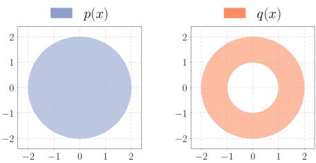
Refer to caption
Figure B.1: Visualization of example distributions for Proposition B.1

Appendix C Discussion of “soft” and “hard” assignments with 1D discrete distributions

In Section 4.2 we considered the “soft-assignment” relaxed OT problem (11) and claimed that for integer β𝛽\beta, the set of minimizers of (11) must contain a “hard-assignment” transportation plan, meaning γij{0,1},i,jsubscript𝛾𝑖𝑗01for-all𝑖𝑗\gamma_{ij}\in\{0,1\},\forall i,j. Below we justify this claim.

Note that for β=0𝛽0\beta=0 the OT problem (11) is the standard OT problem for Wasserstein-1 distance (10), since the inequality constraints i=1mγij1superscriptsubscript𝑖1𝑚subscript𝛾𝑖𝑗1\sum_{i=1}^{m}\gamma_{ij}\leq 1, jfor-all𝑗\forall j can only be satisfied as equalities. For this problem, it is known (e.g. see Peyré et al. (2019) Proposition 2.1) that the set of optimal “soft-assignment” contains a “hard-assignment” represented by a normalized permutation matrix. This fact can be proven using the Birkhoff–von Neumann theorem. The Birkhoff–von Neumann theorem states that the set of doubly stochastic matrices

Pn×n:Pij0,i,j,j=1nPij=1,i,i=1nPij=1,jP\in\mathbb{R}^{n\times n}:\qquad P_{ij}\geq 0,\forall\,i,j,\qquad\sum_{j=1}^{n}P_{ij}=1,\forall\,i,\qquad\sum_{i=1}^{n}P_{ij}=1,\forall\,j

is exactly the set of all finite convex combinations of permutation matrices. In the context of the linear program (11) with β=0𝛽0\beta=0, the Birkhoff–von Neumann theorem means that all extreme points of the polyhedron Γβ(op,oq)subscriptΓ𝛽superscript𝑜𝑝superscript𝑜𝑞\Gamma_{\beta}(o^{p},o^{q}) are hard-assignment matrices. Therefore, by the fundamental theorem of linear programming (Bertsimas & Tsitsiklis, 1997), the minimum of the objective is reached at a “hard-assignment” matrix.

We argue that a similar result holds for the case of integer β>0𝛽0\beta>0. In this case, the matrices in Γβ(op,oq)subscriptΓ𝛽superscript𝑜𝑝superscript𝑜𝑞\Gamma_{\beta}(o^{p},o^{q}) can not be associated with the doubly stochastic matrices, since constraints on of the marginals of γ𝛾\gamma are relaxed to inequality constraints. Because of that, the Birkhoff–von Neumann theorem can not be applied. However, Budish et al. (2009) provide a generalization of the Birkhoff–von Neumann theorem (Theorem 1 in (Budish et al., 2009)) which applies to the cases where the equality constraints are replaced with integer-valued inequality constraints (recall that we consider integer β𝛽\beta). Using this generalized result, our claim can be proven by performing the following steps.

Clearly, the polyhedron Γβ(op,oq)subscriptΓ𝛽superscript𝑜𝑝superscript𝑜𝑞\Gamma_{\beta}(o^{p},o^{q}) contains all “hard-assignment” matrices and all their finite convex combinations. The result proven in (Budish et al., 2009) implies that each element of Γβ(op,oq)subscriptΓ𝛽superscript𝑜𝑝superscript𝑜𝑞\Gamma_{\beta}(o^{p},o^{q}) can be represented as a finite convex combination of “hard-assignment” matrices. Thus, the polyhedron Γβ(op,oq)subscriptΓ𝛽superscript𝑜𝑝superscript𝑜𝑞\Gamma_{\beta}(o^{p},o^{q}) is exactly the set of all finite convex combinations of “hard-assignment” matrices and all extreme points of the polyhedron are “hard-assignment” matrices. Finally, by analogy with the case of β=0𝛽0\beta=0, we invoke the fundamental theorem of the linear programming and conclude that the minimum of the objective (11) is reached at γ𝛾\gamma corresponding to a “hard-assignment” matrix.

Appendix D Experiment details

D.1 USPS to MNIST experiment specifications

We use USPS (Hull, 1994) and MNIST (LeCun et al., 1998) datasets for this adaptation problem.

Following Tachet des Combes et al. (2020) we use LeNet-like (LeCun et al., 1998) architecture for the feature extractor with the 500-dimensional feature representation. The classifier consists of a single linear layer. The discriminator is implemented by a 3-layer MLP with 512 hidden units and leaky-ReLU activation.

We train all methods for 65 0006500065\,000 steps with batch size 646464. We train the feature extractor, the classifier, and the discriminator with SGD (learning rate 0.020.020.02, momentum 0.90.90.9, weight decay 5104)5\cdot 10^{-4}). We perform a single discriminator update per 1 update of the feature extractor and the classifier. After the first 30 0003000030\,000 steps we linearly anneal the feature extractor’s and classifier’s learning rates for 30 0003000030\,000 steps to the final value 21052superscript1052\cdot 10^{-5}.

The feature extractor’s loss is given by a weighted combination of the cross-entropy classification loss on the labeled source example and a domain alignment loss computed from the discriminator’s signal (recall that different method use different forms of the alignment loss). The weight for the classification term is constant and set to λcls=1subscript𝜆cls1\lambda_{\text{cls}}=1. We introduce schedule for the alignment weight λalignsubscript𝜆align\lambda_{\text{align}}. For all alignment methods we linearly increase λalignsubscript𝜆align\lambda_{\text{align}} from 00 to 1.01.01.0 during the first 100001000010000 steps.

For ASA we use history buffers of size 1000.

D.2 STL to CIFAR experiment specifications

We use STL (Coates et al., 2011) and CIFAR-10 (Krizhevsky, 2009) for this adaptation task. STL and CIFAR-10 are both 10-class classification problems. There are 9 common classes between the two datasets. Following Shu et al. (2018) we create a 9-class classification problem by selecting the subsets of examples of the 9 common classes.

For the feature extractor, we adapt the deep CNN architecture of Shu et al. (2018). The feature representation is a 192192192-dimensional vector. The classifier consists of a single linear layer. The discriminator is implemented by a 3-layer MLP with 512 hidden units and leaky-ReLU activation.

We train all methods for 40 0004000040\,000 steps with batch size 646464. We train the feature extractor, the classifier, and the discriminator with ADAM (Kingma & Ba, 2014) (learning rate 0.0010.0010.001, β1=0.5subscript𝛽10.5\beta_{1}=0.5, β2=0.999subscript𝛽20.999\beta_{2}=0.999, no weight decay). We perform a single discriminator update per 1 update of the feature extractor and the classifier.

The weight for the classification loss term is constant and set to λcls=1subscript𝜆cls1\lambda_{\text{cls}}=1. For all alignment methods we use constant alignment weight λalign=0.1subscript𝜆align0.1\lambda_{\text{align}}=0.1.

For ASA we use history buffers of size 1000.

Conditional entropy loss. Following (Shu et al., 2018) we use auxiliary conditional entropy loss on target examples for domain adaptation methods. For a classifier Cϕ:𝒵𝒴:superscript𝐶italic-ϕ𝒵𝒴C^{\phi}:\mathcal{Z}\to\mathcal{Y} and a feature extractor Fθ:𝒳𝒵:superscript𝐹𝜃𝒳𝒵F^{\theta}:\mathcal{X}\to\mathcal{Z} where classifier outputs the distribution over class labels {1,,K}1𝐾\{1,\ldots,K\}

Cϕ(z)K:[Cϕ(z)]k0,k=1K[Cϕ(z)]k=1,C^{\phi}(z)\in\mathbb{R}^{K}:\quad\big{[}C^{\phi}(z)\big{]}_{k}\geq 0,\quad\sum\limits_{k=1}^{K}\big{[}C^{\phi}(z)\big{]}_{k}=1,

the conditional entropy loss on target examples {xiq}i=1Nqsuperscriptsubscriptsuperscriptsubscript𝑥𝑖𝑞𝑖1subscript𝑁𝑞\{x_{i}^{q}\}_{i=1}^{N_{q}} is given by

ent=λent1Nqi=1Nq(k=1K[Cϕ(Fθ(xiq))]klog[Cϕ(Fθ(xiq))]k).\mathcal{L}_{\text{ent}}=\lambda_{\text{ent}}\cdot\frac{1}{N^{q}}\sum_{i=1}^{N_{q}}\Bigg{(}-\sum_{k=1}^{K}\big{[}C^{\phi}(F^{\theta}(x_{i}^{q}))\big{]}_{k}\log\big{[}C^{\phi}(F^{\theta}(x_{i}^{q}))\big{]}_{k}\Bigg{)}. (17)

λentsubscript𝜆ent\lambda_{\text{ent}} is the weight of the conditional entropy loss in the total training objective. This loss acts as an additional regularization of the embeddings of the unlabeled target examples: minimization of the conditional entropy pushes target embeddings away from the classifier’s decision boundary.

For all domain adapation methods we use the conditional entropy loss (17) on target examples with the weight λent=0.1subscript𝜆ent0.1\lambda_{\text{ent}}=0.1.

D.3 Extended experimental results on STL to CIFAR

Effect of conditional entropy loss. In order to quantify the improvements of the support alignment objective and the conditional entropy objective in separation, we conduct an ablation study. In addition to the results reported in Section 5, we evaluate all domain adaptation methods (except VADA which uses the conditional entropy in the original implementation) on STL\toCIFAR task without the conditional entropy loss (λent=0subscript𝜆ent0\lambda_{\text{ent}}=0). The results of the ablation study are presented in Table D.1. We observe that the effect of the auxiliary conditional entropy is essentially the same for all methods across all imbalance levels: with λent=0.1subscript𝜆ent0.1\lambda_{\text{ent}}=0.1 the accuracy either improves (especially the average class accuracy) or roughly stays on the same level. The relative ranking of distribution alignment, relaxed distribution alignment, and support alignment methods is the same with both λent=0subscript𝜆ent0\lambda_{\text{ent}}=0 and λent=0.1subscript𝜆ent0.1\lambda_{\text{ent}}=0.1. The results demonstrate that the benefits of support alignment approach and conditional entropy are orthogonal.

Table D.1: Results of ablation experiments of the effect of auxiliary conditional entropy loss on STL\rightarrowCIFAR data. Same setup and reporting metrics as Table 1.
α=0.0𝛼0.0\alpha=0.0 α=1.0𝛼1.0\alpha=1.0 α=1.5𝛼1.5\alpha=1.5 α=2.0𝛼2.0\alpha=2.0
Algorithm λentsubscript𝜆ent\lambda_{\text{ent}} average min average min average min average min
DANN 0.0 74.674.175.1superscriptsubscript74.674.175.174.6_{~{}74.1}^{~{}75.1} 51.549.955.0superscriptsubscript51.549.955.051.5_{~{}49.9}^{~{}55.0} 68.467.069.2superscriptsubscript68.467.069.268.4_{~{}67.0}^{~{}69.2} 43.241.243.7superscriptsubscript43.241.243.743.2_{~{}41.2}^{~{}43.7} 65.762.865.9superscriptsubscript65.762.865.965.7_{~{}62.8}^{~{}65.9} 35.529.636.2superscriptsubscript35.529.636.235.5_{~{}29.6}^{~{}36.2} 62.560.064.6superscriptsubscript62.560.064.662.5_{~{}60.0}^{~{}64.6} 27.525.727.5superscriptsubscript27.525.727.527.5_{~{}25.7}^{~{}27.5}
DANN 0.1 75.374.975.4superscriptsubscript75.374.975.475.3_{~{}74.9}^{~{}75.4} 54.654.256.6superscriptsubscript54.654.256.654.6_{~{}54.2}^{~{}56.6} 69.968.670.1superscriptsubscript69.968.670.169.9_{~{}68.6}^{~{}70.1} 44.840.745.1superscriptsubscript44.840.745.144.8_{~{}40.7}^{~{}45.1} 64.963.767.1superscriptsubscript64.963.767.164.9_{~{}63.7}^{~{}67.1} 34.933.936.8superscriptsubscript34.933.936.834.9_{~{}33.9}^{~{}36.8} 63.357.464.8superscriptsubscript63.357.464.863.3_{~{}57.4}^{~{}64.8} 27.021.228.5superscriptsubscript27.021.228.527.0_{~{}21.2}^{~{}28.5}
IWDAN 0.0 70.470.270.7superscriptsubscript70.470.270.770.4_{~{}70.2}^{~{}70.7} 47.246.848.0superscriptsubscript47.246.848.047.2_{~{}46.8}^{~{}48.0} 68.668.468.8superscriptsubscript68.668.468.868.6_{~{}68.4}^{~{}68.8} 43.643.246.3superscriptsubscript43.643.246.343.6_{~{}43.2}^{~{}46.3} 66.766.067.9superscriptsubscript66.766.067.966.7_{~{}66.0}^{~{}67.9} 44.743.346.2superscriptsubscript44.743.346.244.7_{~{}43.3}^{~{}46.2} 63.962.966.1superscriptsubscript63.962.966.163.9_{~{}62.9}^{~{}66.1} 36.532.737.3superscriptsubscript36.532.737.336.5_{~{}32.7}^{~{}37.3}
IWDAN 0.1 69.969.970.7superscriptsubscript69.969.970.769.9_{~{}69.9}^{~{}70.7} 50.547.950.6superscriptsubscript50.547.950.650.5_{~{}47.9}^{~{}50.6} 68.768.669.1superscriptsubscript68.768.669.168.7_{~{}68.6}^{~{}69.1} 45.844.850.5superscriptsubscript45.844.850.545.8_{~{}44.8}^{~{}50.5} 67.165.967.3superscriptsubscript67.165.967.367.1_{~{}65.9}^{~{}67.3} 44.740.444.8superscriptsubscript44.740.444.844.7_{~{}40.4}^{~{}44.8} 64.463.664.9superscriptsubscript64.463.664.964.4_{~{}63.6}^{~{}64.9} 36.834.537.9superscriptsubscript36.834.537.936.8_{~{}34.5}^{~{}37.9}
IWCDAN 0.0 70.170.070.8superscriptsubscript70.170.070.870.1_{~{}70.0}^{~{}70.8} 50.549.150.8superscriptsubscript50.549.150.850.5_{~{}49.1}^{~{}50.8} 68.668.269.4superscriptsubscript68.668.269.468.6_{~{}68.2}^{~{}69.4} 44.241.245.8superscriptsubscript44.241.245.844.2_{~{}41.2}^{~{}45.8} 66.065.966.0superscriptsubscript66.065.966.066.0_{~{}65.9}^{~{}66.0} 45.043.747.8superscriptsubscript45.043.747.845.0_{~{}43.7}^{~{}47.8} 63.862.364.1superscriptsubscript63.862.364.163.8_{~{}62.3}^{~{}64.1} 37.333.637.7superscriptsubscript37.333.637.737.3_{~{}33.6}^{~{}37.7}
IWCDAN 0.1 70.170.170.2superscriptsubscript70.170.170.270.1_{~{}70.1}^{~{}70.2} 47.842.449.3superscriptsubscript47.842.449.347.8_{~{}42.4}^{~{}49.3} 69.469.169.4superscriptsubscript69.469.169.469.4_{~{}69.1}^{~{}69.4} 47.146.351.3superscriptsubscript47.146.351.347.1_{~{}46.3}^{~{}51.3} 66.165.067.2superscriptsubscript66.165.067.266.1_{~{}65.0}^{~{}67.2} 39.937.740.8superscriptsubscript39.937.740.839.9_{~{}37.7}^{~{}40.8} 64.563.965.1superscriptsubscript64.563.965.164.5_{~{}63.9}^{~{}65.1} 37.035.540.2superscriptsubscript37.035.540.237.0_{~{}35.5}^{~{}40.2}
sDANN-4 0.0 69.468.870.0superscriptsubscript69.468.870.069.4_{~{}68.8}^{~{}70.0} 46.545.149.7superscriptsubscript46.545.149.746.5_{~{}45.1}^{~{}49.7} 69.669.369.7superscriptsubscript69.669.369.769.6_{~{}69.3}^{~{}69.7} 49.147.449.2superscriptsubscript49.147.449.249.1_{~{}47.4}^{~{}49.2} 68.067.868.6superscriptsubscript68.067.868.668.0_{~{}67.8}^{~{}68.6} 48.242.648.8superscriptsubscript48.242.648.848.2_{~{}42.6}^{~{}48.8} 66.364.266.4superscriptsubscript66.364.266.466.3_{~{}64.2}^{~{}66.4} 40.736.642.9superscriptsubscript40.736.642.940.7_{~{}36.6}^{~{}42.9}
sDANN-4 0.1 71.871.772.1superscriptsubscript71.871.772.171.8_{~{}71.7}^{~{}72.1} 52.152.152.8superscriptsubscript52.152.152.852.1_{~{}52.1}^{~{}52.8} 71.170.471.7superscriptsubscript71.170.471.771.1_{~{}70.4}^{~{}71.7} 49.948.151.8superscriptsubscript49.948.151.849.9_{~{}48.1}^{~{}51.8} 69.468.770.0superscriptsubscript69.468.770.069.4_{~{}68.7}^{~{}70.0} 48.643.549.0superscriptsubscript48.643.549.048.6_{~{}43.5}^{~{}49.0} 66.466.267.9superscriptsubscript66.466.267.966.4_{~{}66.2}^{~{}67.9} 39.033.647.1superscriptsubscript39.033.647.139.0_{~{}33.6}^{~{}47.1}
ASA-sq 0.0 69.969.970.3superscriptsubscript69.969.970.369.9_{~{}69.9}^{~{}70.3} 48.046.650.1superscriptsubscript48.046.650.148.0_{~{}46.6}^{~{}50.1} 68.868.668.9superscriptsubscript68.868.668.968.8_{~{}68.6}^{~{}68.9} 47.345.349.3superscriptsubscript47.345.349.347.3_{~{}45.3}^{~{}49.3} 68.167.268.7superscriptsubscript68.167.268.768.1_{~{}67.2}^{~{}68.7} 45.445.247.8superscriptsubscript45.445.247.845.4_{~{}45.2}^{~{}47.8} 65.765.666.4superscriptsubscript65.765.666.465.7_{~{}65.6}^{~{}66.4} 43.641.345.0superscriptsubscript43.641.345.043.6_{~{}41.3}^{~{}45.0}
ASA-sq 0.1 71.771.771.9superscriptsubscript71.771.771.971.7_{~{}71.7}^{~{}71.9} 52.946.753.4superscriptsubscript52.946.753.452.9_{~{}46.7}^{~{}53.4} 70.770.471.0superscriptsubscript70.770.471.070.7_{~{}70.4}^{~{}71.0} 51.646.852.7superscriptsubscript51.646.852.751.6_{~{}46.8}^{~{}52.7} 69.269.269.3superscriptsubscript69.269.269.369.2_{~{}69.2}^{~{}69.3} 45.643.352.0superscriptsubscript45.643.352.045.6_{~{}43.3}^{~{}52.0} 68.167.268.2superscriptsubscript68.167.268.268.1_{~{}67.2}^{~{}68.2} 44.739.845.9superscriptsubscript44.739.845.944.7_{~{}39.8}^{~{}45.9}
ASA-abs 0.0 69.868.970.0superscriptsubscript69.868.970.069.8_{~{}68.9}^{~{}70.0} 45.745.448.0superscriptsubscript45.745.448.045.7_{~{}45.4}^{~{}48.0} 68.468.468.6superscriptsubscript68.468.468.668.4_{~{}68.4}^{~{}68.6} 44.344.046.8superscriptsubscript44.344.046.844.3_{~{}44.0}^{~{}46.8} 67.967.068.1superscriptsubscript67.967.068.167.9_{~{}67.0}^{~{}68.1} 46.640.448.4superscriptsubscript46.640.448.446.6_{~{}40.4}^{~{}48.4} 66.365.766.9superscriptsubscript66.365.766.966.3_{~{}65.7}^{~{}66.9} 41.640.344.9superscriptsubscript41.640.344.941.6_{~{}40.3}^{~{}44.9}
ASA-abs 0.1 71.671.271.7superscriptsubscript71.671.271.771.6_{~{}71.2}^{~{}71.7} 49.048.453.5superscriptsubscript49.048.453.549.0_{~{}48.4}^{~{}53.5} 70.970.871.0superscriptsubscript70.970.871.070.9_{~{}70.8}^{~{}71.0} 49.247.350.0superscriptsubscript49.247.350.049.2_{~{}47.3}^{~{}50.0} 69.669.669.9superscriptsubscript69.669.669.969.6_{~{}69.6}^{~{}69.9} 43.242.149.5superscriptsubscript43.242.149.543.2_{~{}42.1}^{~{}49.5} 67.866.668.2superscriptsubscript67.866.668.267.8_{~{}66.6}^{~{}68.2} 40.935.449.0superscriptsubscript40.935.449.040.9_{~{}35.4}^{~{}49.0}

Comparison with optimal transport based baselines.

We provide additional experimental results comparing our method with OT-based methods for domain adaptation. We implement two OT-based methods which we describe below.

  • The first method is a variant of the max-sliced Wasserstein distance (which was proposed for GAN training by Deshpande et al. (2019)) for domain adaptation. In the table below we refer to this method as DANN-OT. In our implementation DANN-OT minimizes the Wasserstein distance between the pushforward distributions gpsubscriptsuperscript𝑔𝑝g^{*}_{\sharp}p, gqsubscriptsuperscript𝑔𝑞g^{*}_{\sharp}q induced by the optimal log-loss discriminator gsuperscript𝑔g^{*} (4). As discussed in Section 4.2 (paragraph “Distribution alignment”) the computation of the Wasserstein distance between 1D distributions can be implemented efficiently via sorting.

  • The second method is an OT-based variant of DANN which uses a dual Wasserstein discriminator instead of the log-loss discriminator. In the table below we refer to this method as DANN-WGP. This method minimizes the Wasserstein distance in its dual Kantorovich form. We train the discriminator with the Wasserstein dual objective and a gradient penalty proposed to enforce Lipshitz-norm constraint (Gulrajani et al., 2017).

We present the evaluation results of the OT-based methods on STL\toCIFAR domain adaptation task in the Table D.2. Note that the OT-based methods aim to enforce distribution alignment constraints. We observe that the OT-based methods follow the same trend as DANN: they deliver improved accuracy compared to No DA in the balanced setting, but suffer in the imbalanced settings (α>0𝛼0\alpha>0) due to their distribution alignment nature.

Table D.2: Results of comparison with optimal transport based methods on STL\rightarrowCIFAR data. Same setup and reporting metrics as Table 1.
α=0.0𝛼0.0\alpha=0.0 α=1.0𝛼1.0\alpha=1.0 α=1.5𝛼1.5\alpha=1.5 α=2.0𝛼2.0\alpha=2.0
Algorithm average min average min average min average min
No DA 69.969.870.0superscriptsubscript69.969.870.069.9_{~{}69.8}^{~{}70.0} 49.845.350.6superscriptsubscript49.845.350.649.8_{~{}45.3}^{~{}50.6} 68.868.369.3superscriptsubscript68.868.369.368.8_{~{}68.3}^{~{}69.3} 47.245.348.2superscriptsubscript47.245.348.247.2_{~{}45.3}^{~{}48.2} 66.866.467.2superscriptsubscript66.866.467.266.8_{~{}66.4}^{~{}67.2} 46.045.847.0superscriptsubscript46.045.847.046.0_{~{}45.8}^{~{}47.0} 65.864.866.7superscriptsubscript65.864.866.765.8_{~{}64.8}^{~{}66.7} 43.741.644.6superscriptsubscript43.741.644.643.7_{~{}41.6}^{~{}44.6}
DANN 75.374.975.4superscriptsubscript75.374.975.475.3_{~{}74.9}^{~{}75.4} 54.654.256.6superscriptsubscript54.654.256.654.6_{~{}54.2}^{~{}56.6} 69.968.670.1superscriptsubscript69.968.670.169.9_{~{}68.6}^{~{}70.1} 44.840.745.1superscriptsubscript44.840.745.144.8_{~{}40.7}^{~{}45.1} 64.963.767.1superscriptsubscript64.963.767.164.9_{~{}63.7}^{~{}67.1} 34.933.936.8superscriptsubscript34.933.936.834.9_{~{}33.9}^{~{}36.8} 63.357.464.8superscriptsubscript63.357.464.863.3_{~{}57.4}^{~{}64.8} 27.021.228.5superscriptsubscript27.021.228.527.0_{~{}21.2}^{~{}28.5}
DANN-OT 76.075.876.0superscriptsubscript76.075.876.076.0_{~{}75.8}^{~{}76.0} 55.254.355.5superscriptsubscript55.254.355.555.2_{~{}54.3}^{~{}55.5} 67.767.168.9superscriptsubscript67.767.168.967.7_{~{}67.1}^{~{}68.9} 43.036.543.7superscriptsubscript43.036.543.743.0_{~{}36.5}^{~{}43.7} 64.560.965.1superscriptsubscript64.560.965.164.5_{~{}60.9}^{~{}65.1} 34.429.334.6superscriptsubscript34.429.334.634.4_{~{}29.3}^{~{}34.6} 61.354.462.0superscriptsubscript61.354.462.061.3_{~{}54.4}^{~{}62.0} 24.323.225.5superscriptsubscript24.323.225.524.3_{~{}23.2}^{~{}25.5}
DANN-WGP 74.874.775.1superscriptsubscript74.874.775.174.8_{~{}74.7}^{~{}75.1} 53.553.354.4superscriptsubscript53.553.354.453.5_{~{}53.3}^{~{}54.4} 67.765.367.9superscriptsubscript67.765.367.967.7_{~{}65.3}^{~{}67.9} 38.634.441.0superscriptsubscript38.634.441.038.6_{~{}34.4}^{~{}41.0} 63.357.163.4superscriptsubscript63.357.163.463.3_{~{}57.1}^{~{}63.4} 27.026.332.4superscriptsubscript27.026.332.427.0_{~{}26.3}^{~{}32.4} 59.054.361.8superscriptsubscript59.054.361.859.0_{~{}54.3}^{~{}61.8} 21.918.622.5superscriptsubscript21.918.622.521.9_{~{}18.6}^{~{}22.5}
sDANN-4 71.871.772.1superscriptsubscript71.871.772.171.8_{~{}71.7}^{~{}72.1} 52.152.152.8superscriptsubscript52.152.152.852.1_{~{}52.1}^{~{}52.8} 71.170.471.7superscriptsubscript71.170.471.771.1_{~{}70.4}^{~{}71.7} 49.948.151.8superscriptsubscript49.948.151.849.9_{~{}48.1}^{~{}51.8} 69.468.770.0superscriptsubscript69.468.770.069.4_{~{}68.7}^{~{}70.0} 48.643.549.0superscriptsubscript48.643.549.048.6_{~{}43.5}^{~{}49.0} 66.466.267.9superscriptsubscript66.466.267.966.4_{~{}66.2}^{~{}67.9} 39.033.647.1superscriptsubscript39.033.647.139.0_{~{}33.6}^{~{}47.1}
ASA-sq 71.771.771.9superscriptsubscript71.771.771.971.7_{~{}71.7}^{~{}71.9} 52.946.753.4superscriptsubscript52.946.753.452.9_{~{}46.7}^{~{}53.4} 70.770.471.0superscriptsubscript70.770.471.070.7_{~{}70.4}^{~{}71.0} 51.646.852.7superscriptsubscript51.646.852.751.6_{~{}46.8}^{~{}52.7} 69.269.269.3superscriptsubscript69.269.269.369.2_{~{}69.2}^{~{}69.3} 45.643.352.0superscriptsubscript45.643.352.045.6_{~{}43.3}^{~{}52.0} 68.167.268.2superscriptsubscript68.167.268.268.1_{~{}67.2}^{~{}68.2} 44.739.845.9superscriptsubscript44.739.845.944.7_{~{}39.8}^{~{}45.9}
ASA-abs 71.671.271.7superscriptsubscript71.671.271.771.6_{~{}71.2}^{~{}71.7} 49.048.453.5superscriptsubscript49.048.453.549.0_{~{}48.4}^{~{}53.5} 70.970.871.0superscriptsubscript70.970.871.070.9_{~{}70.8}^{~{}71.0} 49.247.350.0superscriptsubscript49.247.350.049.2_{~{}47.3}^{~{}50.0} 69.669.669.9superscriptsubscript69.669.669.969.6_{~{}69.6}^{~{}69.9} 43.242.149.5superscriptsubscript43.242.149.543.2_{~{}42.1}^{~{}49.5} 67.866.668.2superscriptsubscript67.866.668.267.8_{~{}66.6}^{~{}68.2} 40.935.449.0superscriptsubscript40.935.449.040.9_{~{}35.4}^{~{}49.0}

We would also like to make a comment on OT-based relaxed distribution alignment. Wu et al. (2019b) propose method WDANN-β𝛽\beta which minimizes the dual form of the asymmetrically-relaxed Wasserstein distance. However, they observe that sDANN-β𝛽\beta outperforms WDANN-β𝛽\beta in experiments. Hence, we use sDANN-β𝛽\beta as a relaxed distribution alignment baseline in our experiments.

Effect of alignment weight. We provide additional experimental results comparing ASA with DANN and VADA across different values of the alignment loss weight λalignsubscript𝜆align\lambda_{\text{align}} on STL\toCIFAR task. The results are shown in Table D.3. DANN with a higher alignment weight λalign=1.0subscript𝜆align1.0\lambda_{\text{align}}=1.0 performs better in the balanced (α=0𝛼0\alpha=0) setting and worse in the imbalanced (α>0𝛼0\alpha>0) setting compared to a lower weight λalign=0.1subscript𝜆align0.1\lambda_{\text{align}}=0.1, as the distribution alignment constraint is enforced stricter. VADA optimizes a combination of distribution alignment + VAT (virtual adversarial training) objectives (Shu et al., 2018), and we observe the same trend: with lower alignment weight λalign=0.01subscript𝜆align0.01\lambda_{\text{align}}=0.01, VADA performs worse in the balanced setting and better in the imbalanced setting compared to a higher weight λalign=0.1subscript𝜆align0.1\lambda_{\text{align}}=0.1. Weight λalign=0.1subscript𝜆align0.1\lambda_{\text{align}}=0.1 is a middle ground between having poor performance in the imbalanced setting (λalign=1.0subscript𝜆align1.0\lambda_{\text{align}}=1.0) and not sufficiently enforcing distribution alignment (λalign=0.01subscript𝜆align0.01\lambda_{\text{align}}=0.01).

The role of VAT (similarly to that of conditional entropy loss) is orthogonal to alignment objectives. Thus, we provide additional evaluations of combining support alignment and VAT (the “ASA-sq + VAT” entry in Table D.3) with alignment weight λalign=1.0subscript𝜆align1.0\lambda_{\text{align}}=1.0. The good performance of such combination shows that:

  • One could improve our current support alignment performance by using auxiliary objectives.

  • Support alignment based method performs qualitatively different from distribution alignment based method, since the performance holds with stricter support alignment while distribution alignment needs to loosen the constraints considerably to reduce the performance degradation in the imbalanced setting.

Table D.3: Results of comparison of ASA with DANN and VADA across different values of the alignment loss weight λalignsubscript𝜆align\lambda_{\text{align}} on STL\rightarrowCIFAR data. Same setup and reporting metrics as Table 1.
α=0.0𝛼0.0\alpha=0.0 α=1.0𝛼1.0\alpha=1.0 α=1.5𝛼1.5\alpha=1.5 α=2.0𝛼2.0\alpha=2.0
Algorithm λalignsubscript𝜆align\lambda_{\text{align}} average min average min average min average min
DANN 0.01 72.372.272.7superscriptsubscript72.372.272.772.3_{~{}72.2}^{~{}72.7} 49.548.850.8superscriptsubscript49.548.850.849.5_{~{}48.8}^{~{}50.8} 70.669.771.2superscriptsubscript70.669.771.270.6_{~{}69.7}^{~{}71.2} 48.941.551.2superscriptsubscript48.941.551.248.9_{~{}41.5}^{~{}51.2} 68.567.268.7superscriptsubscript68.567.268.768.5_{~{}67.2}^{~{}68.7} 46.136.250.0superscriptsubscript46.136.250.046.1_{~{}36.2}^{~{}50.0} 65.964.166.0superscriptsubscript65.964.166.065.9_{~{}64.1}^{~{}66.0} 36.729.939.4superscriptsubscript36.729.939.436.7_{~{}29.9}^{~{}39.4}
DANN 0.1 75.374.975.4superscriptsubscript75.374.975.475.3_{~{}74.9}^{~{}75.4} 54.654.256.6superscriptsubscript54.654.256.654.6_{~{}54.2}^{~{}56.6} 69.968.670.1superscriptsubscript69.968.670.169.9_{~{}68.6}^{~{}70.1} 44.840.745.1superscriptsubscript44.840.745.144.8_{~{}40.7}^{~{}45.1} 64.963.767.1superscriptsubscript64.963.767.164.9_{~{}63.7}^{~{}67.1} 34.933.936.8superscriptsubscript34.933.936.834.9_{~{}33.9}^{~{}36.8} 63.357.464.8superscriptsubscript63.357.464.863.3_{~{}57.4}^{~{}64.8} 27.021.228.5superscriptsubscript27.021.228.527.0_{~{}21.2}^{~{}28.5}
DANN 1.0 77.276.877.3superscriptsubscript77.276.877.377.2_{~{}76.8}^{~{}77.3} 58.556.759.4superscriptsubscript58.556.759.458.5_{~{}56.7}^{~{}59.4} 66.364.566.8superscriptsubscript66.364.566.866.3_{~{}64.5}^{~{}66.8} 37.937.541.6superscriptsubscript37.937.541.637.9_{~{}37.5}^{~{}41.6} 62.856.163.3superscriptsubscript62.856.163.362.8_{~{}56.1}^{~{}63.3} 27.524.628.9superscriptsubscript27.524.628.927.5_{~{}24.6}^{~{}28.9} 58.752.359.7superscriptsubscript58.752.359.758.7_{~{}52.3}^{~{}59.7} 18.517.220.5superscriptsubscript18.517.220.518.5_{~{}17.2}^{~{}20.5}
VADA 0.01 74.474.274.4superscriptsubscript74.474.274.474.4_{~{}74.2}^{~{}74.4} 54.252.655.4superscriptsubscript54.252.655.454.2_{~{}52.6}^{~{}55.4} 71.771.771.7superscriptsubscript71.771.771.771.7_{~{}71.7}^{~{}71.7} 51.645.052.0superscriptsubscript51.645.052.051.6_{~{}45.0}^{~{}52.0} 69.568.469.7superscriptsubscript69.568.469.769.5_{~{}68.4}^{~{}69.7} 47.540.049.8superscriptsubscript47.540.049.847.5_{~{}40.0}^{~{}49.8} 65.964.866.1superscriptsubscript65.964.866.165.9_{~{}64.8}^{~{}66.1} 37.235.339.4superscriptsubscript37.235.339.437.2_{~{}35.3}^{~{}39.4}
VADA 0.1 76.776.676.7superscriptsubscript76.776.676.776.7_{~{}76.6}^{~{}76.7} 56.953.558.3superscriptsubscript56.953.558.356.9_{~{}53.5}^{~{}58.3} 70.670.071.0superscriptsubscript70.670.071.070.6_{~{}70.0}^{~{}71.0} 47.744.048.8superscriptsubscript47.744.048.847.7_{~{}44.0}^{~{}48.8} 66.165.466.5superscriptsubscript66.165.466.566.1_{~{}65.4}^{~{}66.5} 35.733.339.3superscriptsubscript35.733.339.335.7_{~{}33.3}^{~{}39.3} 63.260.264.7superscriptsubscript63.260.264.763.2_{~{}60.2}^{~{}64.7} 25.525.228.0superscriptsubscript25.525.228.025.5_{~{}25.2}^{~{}28.0}
ASA-sq 0.1 71.771.771.9superscriptsubscript71.771.771.971.7_{~{}71.7}^{~{}71.9} 52.946.753.4superscriptsubscript52.946.753.452.9_{~{}46.7}^{~{}53.4} 70.770.471.0superscriptsubscript70.770.471.070.7_{~{}70.4}^{~{}71.0} 51.646.852.7superscriptsubscript51.646.852.751.6_{~{}46.8}^{~{}52.7} 69.269.269.3superscriptsubscript69.269.269.369.2_{~{}69.2}^{~{}69.3} 45.643.352.0superscriptsubscript45.643.352.045.6_{~{}43.3}^{~{}52.0} 68.167.268.2superscriptsubscript68.167.268.268.1_{~{}67.2}^{~{}68.2} 44.739.845.9superscriptsubscript44.739.845.944.7_{~{}39.8}^{~{}45.9}
ASA-sq + VAT 1.0 74.274.074.5superscriptsubscript74.274.074.574.2_{~{}74.0}^{~{}74.5} 52.251.952.5superscriptsubscript52.251.952.552.2_{~{}51.9}^{~{}52.5} 72.271.972.2superscriptsubscript72.271.972.272.2_{~{}71.9}^{~{}72.2} 53.545.453.6superscriptsubscript53.545.453.653.5_{~{}45.4}^{~{}53.6} 70.670.470.8superscriptsubscript70.670.470.870.6_{~{}70.4}^{~{}70.8} 48.945.652.3superscriptsubscript48.945.652.348.9_{~{}45.6}^{~{}52.3} 67.466.867.7superscriptsubscript67.466.867.767.4_{~{}66.8}^{~{}67.7} 43.039.446.0superscriptsubscript43.039.446.043.0_{~{}39.4}^{~{}46.0}

D.4 VisDA-17 experiment specifications

We use train and validation sets of the VisDA-17 challenge (Peng et al., 2017).

For the feature extractor we use ResNet-50 He et al. (2016) architecture with modified output size of the final linear layer. The feature representation is 256-dimensional vector. We use the weights from pre-trained ResNet-50 model (torchvision model hub) for all layers except the final linear layer. The classifier consists of a single linear layer. The discriminator is implemented by a 3-layer MLP with 1024 hidden units and leaky-ReLU activation.

We train all methods for 50 0005000050\,000 steps with batch size 363636. We train the feature extractor, the classifier, and the discriminator with SGD. For the feature extractor we use learning rate 0.0010.0010.001, momentum 0.90.90.9, weight decay 0.0010.0010.001. For the classifier we use learning rate 0.010.010.01, momentum 0.90.90.9, weight decay 0.0010.0010.001. For the discriminator we use learning rate 0.0050.0050.005, momentum 0.90.90.9, weight decay 0.0010.0010.001. We perform a single discriminator update per 1 update of the feature extractor and the classifier. We linearly anneal the feature extractor’s and classifier’s learning rate throughout the training (50 0005000050\,000) steps. By the end of the training the learning rates of the feature extractor and the classifier are decreased by a factor of 0.050.050.05.

The weight for the classification term is constant and set to λcls=1subscript𝜆cls1\lambda_{\text{cls}}=1. We introduce schedule for the alignment weight λalignsubscript𝜆align\lambda_{\text{align}}. For all alignment methods we linearly increase λalignsubscript𝜆align\lambda_{\text{align}} from 00 to 0.10.10.1 during the first 100001000010000 steps. For all methods we use auxiliary conditional entropy loss on target examples with the weight λent=0.1subscript𝜆ent0.1\lambda_{\text{ent}}=0.1.

For ASA we use history buffers of size 1000.

D.5 History size effect and evaluation of support distance

History size effect. To quantify the effects of mini-batch training mentioned in Section 3, we explore different sizes of history buffers on USPS\toMNIST task with the label distribution shift α=1.5𝛼1.5\alpha=1.5. The results are presented in Figure D.1 and Table D.4. Figure D.2 shows the distributions of outputs of the learned discriminator at the end of the training. While without any alignment objectives neither the densities nor the supports of gψpZθsubscriptsuperscript𝑔𝜓subscriptsuperscript𝑝𝜃𝑍{g^{\psi}}_{\sharp}p^{\theta}_{Z} and gψqZθsubscriptsuperscript𝑔𝜓subscriptsuperscript𝑞𝜃𝑍{g^{\psi}}_{\sharp}q^{\theta}_{Z} are aligned, both alignment methods approximately satisfy their respective alignment constraints. Compared with DANN results, ASA with small history size performs similarly to distribution alignment, while all history sizes are enough for support alignment. We also observe the correlation between distribution distance and target accuracy: under label distribution shifts, the better distribution alignment is achieved, the more target accuracy suffers. Note that with too big history buffers (e.g. n=5000𝑛5000n=5000), we observe a sudden drop in performance and increases in distances. We hypothesize that this could be caused by the fact that the history buffer stores discriminator output values from the past steps while the discriminator parameters constantly evolve during training. As a result, for a large history buffer, the older items might no longer accurately represent the current pushforward distribution as they become outdated.

Refer to caption
Figure D.1: Evaluation of history size effect for ASA on MNIST\toUSPS with the label distribution shift (α=1.5𝛼1.5\alpha=1.5). The panels show (left to right): minimum class accuracy on target test set; Wasserstein distance 𝒟W(gψpZθ,gψqZθ)subscript𝒟𝑊subscriptsuperscript𝑔𝜓subscriptsuperscript𝑝𝜃𝑍subscriptsuperscript𝑔𝜓subscriptsuperscript𝑞𝜃𝑍\mathcal{D}_{W}({g^{\psi}}_{\sharp}p^{\theta}_{Z},{g^{\psi}}_{\sharp}q^{\theta}_{Z}) between the pushforward distributions of source and target representations induced by the discriminator; SSD divergence 𝒟(gψpZθ,gψqZθ)subscript𝒟subscriptsuperscript𝑔𝜓subscriptsuperscript𝑝𝜃𝑍subscriptsuperscript𝑔𝜓subscriptsuperscript𝑞𝜃𝑍\mathcal{D}_{\triangle}({g^{\psi}}_{\sharp}p^{\theta}_{Z},{g^{\psi}}_{\sharp}q^{\theta}_{Z}) between the pushforward distributions. In each panel the dashed lines show the respective quantities for “No DA” and DANN methods.

Direct evaluation of support distance. In order to directly evaluate the ability of ASA (with history buffers) to enforce support alignment, we consider the setting of the illustrative experiment described in Section 5 (3-class USPS\toMNIST adaptation with 2D feature extractor, α=1.5𝛼1.5\alpha=1.5). We compare methods No DA, DANN, and ASA-abs (with different history buffer sizes). For each method we consider the embedding space of the learned feature extractor at the end of training and compute Wasserstein distance 𝒟W(pZθ,qZθ)subscript𝒟𝑊subscriptsuperscript𝑝𝜃𝑍subscriptsuperscript𝑞𝜃𝑍\mathcal{D}_{W}(p^{\theta}_{Z},q^{\theta}_{Z}) and SSD divergence 𝒟(pZθ,qZθ)subscript𝒟subscriptsuperscript𝑝𝜃𝑍subscriptsuperscript𝑞𝜃𝑍\mathcal{D}_{\triangle}(p^{\theta}_{Z},q^{\theta}_{Z}) between the embeddings of source and target domain (note that we compute the distances in the original embedding space directly without projecting data to 1D with the discriminator). To ensure meaningful comparison of the distances between different embedding spaces, we apply a global affine transformation for each embedding space: we center the embeddings so that their average is 0 and re-scale them so that their average norm is 1. The results of this evaluation are shown in Table D.5. We observe that, compared to no alignment and distribution alignment (DANN) methods, ASA aligns the supports without necessarily aligning the distributions (in this imbalanced setting, distribution alignment implies low adaptation accuracy).

Table D.4: Analysis of effect history size parameter for ASA on USPS\toMNIST with class label distribution shift corresponding to α=1.5𝛼1.5\alpha=1.5. We report distribution and support distances between the pushforward distributions gψpZθsubscriptsuperscript𝑔𝜓subscriptsuperscript𝑝𝜃𝑍{g^{\psi}}_{\sharp}p^{\theta}_{Z} and gψqZθsubscriptsuperscript𝑔𝜓subscriptsuperscript𝑞𝜃𝑍{g^{\psi}}_{\sharp}q^{\theta}_{Z}, as well as the value of discriminator’s log-loss.
Target accuracy (%) Distribution distances
Method History size average min 𝒟W(gψpZθ,gψqZθ)subscript𝒟𝑊subscriptsuperscript𝑔𝜓subscriptsuperscript𝑝𝜃𝑍subscriptsuperscript𝑔𝜓subscriptsuperscript𝑞𝜃𝑍\mathcal{D}_{W}({g^{\psi}}_{\sharp}p^{\theta}_{Z},{g^{\psi}}_{\sharp}q^{\theta}_{Z}) 𝒟(gψpZθ,gψqZθ)subscript𝒟subscriptsuperscript𝑔𝜓subscriptsuperscript𝑝𝜃𝑍subscriptsuperscript𝑔𝜓subscriptsuperscript𝑞𝜃𝑍\mathcal{D}_{\triangle}({g^{\psi}}_{\sharp}p^{\theta}_{Z},{g^{\psi}}_{\sharp}q^{\theta}_{Z}) Log-loss
No DA 71.2871.2572.51superscriptsubscript71.2871.2572.5171.28_{~{}71.25}^{~{}72.51} 27.4624.2137.26superscriptsubscript27.4624.2137.2627.46_{~{}24.21}^{~{}37.26} 307.56277.33322.00superscriptsubscript307.56277.33322.00307.56_{~{}277.33}^{~{}322.00} 40.3532.1046.06superscriptsubscript40.3532.1046.0640.35_{~{}32.10}^{~{}46.06} 00.0500.0400.07superscriptsubscript00.0500.0400.0700.05_{~{}00.04}^{~{}00.07}
DANN 69.9663.8971.25superscriptsubscript69.9663.8971.2569.96_{~{}63.89}^{~{}71.25} 01.1100.9901.53superscriptsubscript01.1100.9901.5301.11_{~{}00.99}^{~{}01.53} 00.1100.1000.11superscriptsubscript00.1100.1000.1100.11_{~{}00.10}^{~{}00.11} 00.0000.0000.00superscriptsubscript00.0000.0000.0000.00_{~{}00.00}^{~{}00.00} 00.6500.6500.65superscriptsubscript00.6500.6500.6500.65_{~{}00.65}^{~{}00.65}
ASA-abs 0 62.7561.7864.35superscriptsubscript62.7561.7864.3562.75_{~{}61.78}^{~{}64.35} 19.3617.9023.63superscriptsubscript19.3617.9023.6319.36_{~{}17.90}^{~{}23.63} 01.0700.9901.15superscriptsubscript01.0700.9901.1501.07_{~{}00.99}^{~{}01.15} 00.0100.0000.01superscriptsubscript00.0100.0000.0100.01_{~{}00.00}^{~{}00.01} 00.5700.5600.58superscriptsubscript00.5700.5600.5800.57_{~{}00.56}^{~{}00.58}
ASA-abs 100 80.5878.2281.73superscriptsubscript80.5878.2281.7380.58_{~{}78.22}^{~{}81.73} 35.0932.1044.37superscriptsubscript35.0932.1044.3735.09_{~{}32.10}^{~{}44.37} 02.6402.1502.70superscriptsubscript02.6402.1502.7002.64_{~{}02.15}^{~{}02.70} 00.0000.0000.00superscriptsubscript00.0000.0000.0000.00_{~{}00.00}^{~{}00.00} 00.5300.5200.53superscriptsubscript00.5300.5200.5300.53_{~{}00.52}^{~{}00.53}
ASA-abs 500 92.0290.5692.76superscriptsubscript92.0290.5692.7692.02_{~{}90.56}^{~{}92.76} 76.9670.9483.72superscriptsubscript76.9670.9483.7276.96_{~{}70.94}^{~{}83.72} 06.2105.6906.48superscriptsubscript06.2105.6906.4806.21_{~{}05.69}^{~{}06.48} 00.0000.0000.01superscriptsubscript00.0000.0000.0100.00_{~{}00.00}^{~{}00.01} 00.4500.4500.45superscriptsubscript00.4500.4500.4500.45_{~{}00.45}^{~{}00.45}
ASA-abs 1000 92.5490.9092.93superscriptsubscript92.5490.9092.9392.54_{~{}90.90}^{~{}92.93} 82.4174.5385.43superscriptsubscript82.4174.5385.4382.41_{~{}74.53}^{~{}85.43} 08.0607.9708.19superscriptsubscript08.0607.9708.1908.06_{~{}07.97}^{~{}08.19} 00.0100.0100.02superscriptsubscript00.0100.0100.0200.01_{~{}00.01}^{~{}00.02} 00.4100.4000.41superscriptsubscript00.4100.4000.4100.41_{~{}00.40}^{~{}00.41}
ASA-abs 5000 86.0384.8687.50superscriptsubscript86.0384.8687.5086.03_{~{}84.86}^{~{}87.50} 62.1946.9871.62superscriptsubscript62.1946.9871.6262.19_{~{}46.98}^{~{}71.62} 29.2324.5429.63superscriptsubscript29.2324.5429.6329.23_{~{}24.54}^{~{}29.63} 00.0500.0500.08superscriptsubscript00.0500.0500.0800.05_{~{}00.05}^{~{}00.08} 00.2900.2900.30superscriptsubscript00.2900.2900.3000.29_{~{}00.29}^{~{}00.30}
Refer to caption
(a) No DA
Refer to caption
(b) DANN
Refer to caption
(c) ASA (n=0𝑛0n=0)
Refer to caption
(d) ASA (n=1000𝑛1000n=1000)
Figure D.2: Kernel density estimates (in the discriminator output space) of gψpZθsubscriptsuperscript𝑔𝜓subscriptsuperscript𝑝𝜃𝑍{g^{\psi}}_{\sharp}p^{\theta}_{Z}, gψqZθsubscriptsuperscript𝑔𝜓subscriptsuperscript𝑞𝜃𝑍{g^{\psi}}_{\sharp}q^{\theta}_{Z} at the end of the training on USPS\toMNIST task with α=1.5𝛼1.5\alpha=1.5. n𝑛n is the size of ASA history buffers.
Table D.5: Results of No DA, DANN, and ASA-abs (with different history sizes) on 3-class USPS\toMNIST adaptation with 2D feature extractor and label distribution shift corresponding to α=1.5𝛼1.5\alpha=1.5. We report average and minimum target class accuracy, as well as Wasserstein distance 𝒟Wsubscript𝒟𝑊\mathcal{D}_{W} and support divergence 𝒟subscript𝒟\mathcal{D}_{\triangle} between source pZθsubscriptsuperscript𝑝𝜃𝑍p^{\theta}_{Z} and target qZθsubscriptsuperscript𝑞𝜃𝑍q^{\theta}_{Z} 2D embedding distributions. We report median (the main number), and 25 (subscript) and 75 (superscript) percentiles across 5 runs.
Algorithm History size Accuracy (avg) Accuracy (min) 𝒟W(pZθ,qZθ)subscript𝒟𝑊subscriptsuperscript𝑝𝜃𝑍subscriptsuperscript𝑞𝜃𝑍\mathcal{D}_{W}(p^{\theta}_{Z},q^{\theta}_{Z}) 𝒟(pZθ,qZθ)subscript𝒟subscriptsuperscript𝑝𝜃𝑍subscriptsuperscript𝑞𝜃𝑍\mathcal{D}_{\triangle}(p^{\theta}_{Z},q^{\theta}_{Z})
No DA 63.062.369.6superscriptsubscript63.062.369.663.0_{~{}62.3}^{~{}69.6} 45.337.953.6superscriptsubscript45.337.953.645.3_{~{}37.9}^{~{}53.6} 0.7800.7500.84superscriptsubscript0.7800.7500.840.78_{~{}00.75}^{~{}00.84} 0.100.100.10superscriptsubscript0.100.100.100.10_{~{}0.10}^{~{}0.10}
DANN 75.672.483.7superscriptsubscript75.672.483.775.6_{~{}72.4}^{~{}83.7} 54.849.655.1superscriptsubscript54.849.655.154.8_{~{}49.6}^{~{}55.1} 0.070.060.08superscriptsubscript0.070.060.080.07_{~{}0.06}^{~{}0.08} 0.020.020.02superscriptsubscript0.020.020.020.02_{~{}0.02}^{~{}0.02}
ASA-abs 0 73.973.484.1superscriptsubscript73.973.484.173.9_{~{}73.4}^{~{}84.1} 61.854.672.4superscriptsubscript61.854.672.461.8_{~{}54.6}^{~{}72.4} 0.230.220.47superscriptsubscript0.230.220.470.23_{~{}0.22}^{~{}0.47} 0.030.030.03superscriptsubscript0.030.030.030.03_{~{}0.03}^{~{}0.03}
ASA-abs 100 88.586.895.1superscriptsubscript88.586.895.188.5_{~{}86.8}^{~{}95.1} 71.470.693.3superscriptsubscript71.470.693.371.4_{~{}70.6}^{~{}93.3} 0.540.560.36superscriptsubscript0.540.560.360.54_{~{}0.56}^{~{}0.36} 0.030.030.03superscriptsubscript0.030.030.030.03_{~{}0.03}^{~{}0.03}
ASA-abs 500 94.588.794.7superscriptsubscript94.588.794.794.5_{~{}88.7}^{~{}94.7} 89.083.190.3superscriptsubscript89.083.190.389.0_{~{}83.1}^{~{}90.3} 0.590.550.64superscriptsubscript0.590.550.640.59_{~{}0.55}^{~{}0.64} 0.030.030.03superscriptsubscript0.030.030.030.03_{~{}0.03}^{~{}0.03}
ASA-abs 1000 91.191.193.0superscriptsubscript91.191.193.091.1_{~{}91.1}^{~{}93.0} 85.680.786.2superscriptsubscript85.680.786.285.6_{~{}80.7}^{~{}86.2} 0.590.550.62superscriptsubscript0.590.550.620.59_{~{}0.55}^{~{}0.62} 0.030.030.03superscriptsubscript0.030.030.030.03_{~{}0.03}^{~{}0.03}
ASA-abs 2000 94.091.294.7superscriptsubscript94.091.294.794.0_{~{}91.2}^{~{}94.7} 88.680.289.4superscriptsubscript88.680.289.488.6_{~{}80.2}^{~{}89.4} 0.620.580.66superscriptsubscript0.620.580.660.62_{~{}0.58}^{~{}0.66} 0.030.030.03superscriptsubscript0.030.030.030.03_{~{}0.03}^{~{}0.03}
ASA-abs 5000 82.181.883.9superscriptsubscript82.181.883.982.1_{~{}81.8}^{~{}83.9} 68.965.570.9superscriptsubscript68.965.570.968.9_{~{}65.5}^{~{}70.9} 0.640.630.67superscriptsubscript0.640.630.670.64_{~{}0.63}^{~{}0.67} 0.040.040.04superscriptsubscript0.040.040.040.04_{~{}0.04}^{~{}0.04}