Finite-Length Scaling of SC-LDPC Codes
With a Limited Number of Decoding Iterations
Abstract
We propose four finite-length scaling laws to predict the frame error rate (FER) performance of spatially-coupled low-density parity-check codes under full belief propagation (BP) decoding with a limit on the number of decoding iterations and a scaling law for sliding window decoding, also with limited iterations. The laws for full BP decoding provide a choice between accuracy and computational complexity; a good balance between them is achieved by the law that models the number of decoded bits after a certain number of BP iterations by a time-integrated Ornstein-Uhlenbeck process. This framework is developed further to model sliding window decoding as a race between the integrated Ornstein-Uhlenbeck process and an absorbing barrier that corresponds to the left boundary of the sliding window. The proposed scaling laws yield accurate FER predictions.
Index Terms:
Codes-on-graphs, finite-length code performance, spatially coupled LDPC codes, window decodingI Introduction
Spatially-coupled low-density parity-check (SC-LDPC) codes [1, 2] achieve capacity under suboptimal yet computationally feasible belief propagation (BP) decoding, which was first observed numerically [2], then proved for the binary erasure channel (BEC) [3] and later for the broad class of binary-input memoryless symmetric channels [4]. Moreover, it was shown that the minimum distance of regular SC-LDPC code ensembles grows linearly with the block length [5]. Spatial coupling is also a powerful technique more broadly; it has been applied to, e.g., turbo-like codes [6], product-like codes [7], lossy compression [8], and compressed sensing [9].
The Tanner graph of an SC-LDPC code is constructed by arranging the Tanner graphs of several uncoupled LDPC codes into a sequence and interconnecting them according to a predefined pattern. The interconnecting is done in such a way so as to create structured irregularity at the boundaries of the resulting chain, such that the bits at the boundaries are better protected than those in the middle of the chain and are more likely to be decoded successfully; during BP decoding, information propagates from those boundaries inward in a wave-like fashion.
The structured irregularity at the boundaries entails a loss in code rate. The rate loss goes to zero as the chain length grows, but so does the probability that the decoding waves fail to propagate through the entire chain. A longer chain also implies higher latency if BP decoding is performed on the whole received sequence, a scheme we refer to as full BP. To limit decoding latency, so-called sliding window decoding, originally proposed in [10], is used in practice. Sliding window decoding limits BP decoding to a window of several spatial positions that slides through the chain from the left boundary rightward, making a decision on the bits that leave the window along the way and thus limiting decoding latency to the size of the window. Further, due to constraints on decoding latency and energy efficiency, both full BP and sliding window decoding must in practice be limited in terms of the maximum number of BP iterations.
To adopt an SC-LDPC code in a practical setting, the system designer would have to specify a range of parameters, including the underlying LDPC code ensemble, the interconnecting pattern, the length of the coupled chain, the size of the sliding window, and the limit on the number of decoding iterations. It is therefore important to understand the influence of these parameters on the error-correcting performance, which is the subject of ongoing scientific inquiry.
The asymptotic performance of SC-LDPC codes (i.e., when the block length of the component LDPC codes grows large) is relatively well understood. Much less is known about their finite-length behavior. Olmos and Urbanke proposed a finite-length scaling law to predict the frame error rate (FER) of SC-LDPC code ensembles under full BP decoding with an unlimited number of iterations over the BEC [11]. The law in [11] follows the approach proposed earlier in [12] for uncoupled LDPC code ensembles and focuses on the number of degree-one check nodes (CNs) available for peeling decoding. Peeling decoding is equivalent in error-correcting performance to BP decoding with unlimited iterations but is more tractable analytically. A decoding failure corresponds to the peeling decoder running out of degree-one CNs before recovering the entire codeword. The authors estimate the probability of that event using an exponential approximation to the first-hit time distribution of an appropriately chosen Ornstein-Uhlenbeck process [11]. This framework was later applied to protograph-based [13] and generalized [14] SC-LDPC code ensembles.
The prediction in [11] captures the slope of the FER curve well. However, it exhibits a gap to the simulated FER performance. In [15], we closed this gap by proposing an alternative scaling law that models the number of degree-one CNs available for peeling decoding as a sum of two independent Ornstein-Uhlenbeck processes that correspond to the decoding waves from the left and right boundary of the chain. We provided laws to also predict the bit and block error rate performance. Importantly for practical applications, we proposed scaling laws for the frame, bit, and block error rate under sliding window decoding, albeit still in the case of unlimited number of iterations.
The scaling law for the FER under full BP decoding from [15] was used in [16] to elucidate the non-trivial space of trade-offs associated with the choice of code parameters and extended in [17] to predict the error rate performance of periodically-doped SC-LDPC code ensembles for streaming. In [18], the authors optimize protograph-based SC-LDPC code constructions under sliding window decoding using a criterion derived from finite-length scaling models (the so-called window mean parameter); they show that taking into account the finite-length scaling behavior of SC-LDPC code ensembles during code optimization can yield codes that significantly outperform their counterparts designed using asymptotic BP thresholds only.
Our ambition is to make finite-length scaling laws the tool of choice in such code parameter optimization. To that end, this paper tackles the problem of predicting the FER of SC-LDPC code ensembles over the BEC under both full BP and sliding window decoding for the practical case of a limited number of iterations. First, we consider full BP decoding and propose four scaling laws that vary in accuracy and computational complexity. One of these laws models the number of bits recovered after a certain number of BP iterations by a time-integrated Ornstein-Uhlenbeck process. We then extend this framework and model sliding window decoding as a race between an absorbing barrier that corresponds to the left boundary of the window and an integrated Ornstein-Uhlenbeck process (with an additional diffusion term) that corresponds to the position of the left decoding wave. We estimate the probability of the wave being absorbed at the barrier (and thus overtaken by the sliding window) by numerically solving the initial value problem of the corresponding Fokker-Planck equation with appropriately chosen boundary conditions. The proposed laws yield accurate predictions of the FER and allow us to quantify performance degradation associated with the introduction of the limit on the number of decoding iterations, making practical code parameter optimization using finite-length scaling laws a step closer to reality.
II Preliminaries
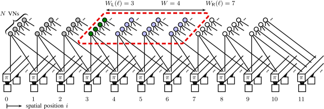
We consider the semi-structured SC-LDPC code ensemble introduced in [11]. Its Tanner graph is shown in Fig. 1. To construct the Tanner graph of an element of the SC-LDPC code ensemble, one must first take Tanner graphs of length- -regular LDPC codes of variable node (VN) degree and CN degree and arrange them into spatial positions indexed by . Each spatial position contains VNs and CNs, where we assume is an integer. We refer to as the component code length and to as the chain length. The set of all VNs in the Tanner graph—and thus of all code bits—is referred to as the frame. The Tanner graphs of the individual (uncoupled) LDPC codes are then interconnected as follows: each VN at position is connected to CNs in positions . Specifically, one CN is chosen uniformly at random among CNs at position , another one at position , and so on until position . To connect the overhanging edges at the end of the chain, additional positions that contain CNs only are appended, resulting in a terminated ensemble. The generation of the elements from this ensemble is described in detail in [11] and can be expressed in terms of choosing the permutation blocks in the Tanner graph in Fig. 1, marked by .
The ensemble is structured from the VN perspective—it is certain that each VN is connected to CNs in different spatial positions. The same cannot be said about the CNs. Indeed, a CN at position can be connected to VNs from any non-empty subset of positions , depending on how the permutation block at position reshuffles the edges connected to VNs at positions (see Fig. 1). This particular “semi-structured” ensemble is proposed in [11] to simplify the analysis. The same approach was later applied to protograph-based ensembles [13].
In addition to the terminated ensemble, we also consider the truncated and unterminated ensembles. In the truncated ensemble, the additional positions with CNs only are not added to the chain of length , and the overhanging edges emanating from VNs at positions are simply deleted from the Tanner graph. The degree of VNs in these last positions is therefore reduced. In the unterminated ensemble, the chain is neither terminated nor truncated, resulting in a “semi-infinite” sequence of coupled codes. We introduce the unterminated ensemble for the analysis of sliding window decoding, and we evaluate the decoding error probability over the first positions of this semi-infinite chain.
Key to impressive error-correcting performance of SC-LDPC codes under BP decoding is the lower degree of CNs at the terminated boundaries of the chain, i.e., at the left boundary of the truncated and unterminated ensembles and at both left and right boundaries of the terminated ensemble. During BP decoding, information propagates from the terminated boundaries of the chain inward in a wave-like fashion. The finite-length scaling laws aim to estimate the probability that such “decoding waves” fail to propagate through the entire chain, which results in decoding error.
Full BP decoding entails a decoding latency of bits, which is impractical for long spatially-coupled chains. To limit decoding latency, sliding window decoding is used in practice, where decoding is limited to VNs in a window of spatial positions (depicted as the red dashed rectangle in Fig. 1). After a certain number of BP iterations, the decoder decides on the values of the bits in the left-most spatial position within the window (colored green in Fig. 1) and the window slides by one position to the right over the Tanner graph. We index BP decoding iterations by and denote the leftmost position of the window by . The first position just outside the window is denoted by , as illustrated in Fig. 1. Sliding window decoding has a decoding latency of bits [10].
This paper investigates the influence of the limit on the number of BP iterations on the error-correcting performance. In the case of full BP decoding, we denote this limit by and treat it is as a parameter of the decoder. In the case of sliding window decoding, the system designer should choose two parameters instead: the number of BP iterations after which the window slides to position 1, i.e., , which we denote by and whose impact will be clarified later, and, for , the number of BP iterations before the window slides further, which we denote by . The total budget of BP iterations in the case of sliding window decoding can be obtained from and for a chain of length as
| (1) |
We consider transmission over the BEC with erasure probability .
II-A Density Evolution
Let denote the probability that a CN at position sends an erasure message to a VN at position at BP iteration . Likewise, let be the probability that a VN at position is erased, and the probability that a VN at position sends an erasure message to a CN at position at BP iteration . The CN update for the semi-structured ensemble averages the incoming error probabilities as
| (2) |
To circumvent the problem of the reduced-degree CNs at the boundaries, the values of that correspond to VN indices outside the chain—i.e., when —are set to zero, implying that the VNs outside the chain are not erased.
Since a VN at position is connected to consecutive positions , as we discussed in the beginning of Section II, the VN update for the semi-structured ensemble is
| (3) |
and the a posteriori probability that a VN at position remains erased at iteration is
| (4) |
II-B Peeling Decoding
The finite-length analysis of BP decoding for the BEC becomes more tractable by considering peeling decoding [19], which is equivalent to BP decoding for an infinite number of iterations. The peeling decoder gets stuck in the same stopping sets and therefore yields the same performance as the BP decoder [19]. At the initial stage of peeling decoding, all VNs that correspond to non-erased bits are removed from the Tanner graph. At every subsequent iteration, the decoder selects one degree-one CN uniformly at random among all degree-one CNs in the graph. Since the value of the code bit associated with the VN connected to the chosen degree-one CN can be recovered, the decoder removes both the CN and VN from the Tanner graph along with adjacent edges and modifies the parity-check equations associated with the adjacent CNs according to the value of the recovered bit. This may in turn create new degree-one CNs to choose from (or remove some other degree-one CNs collaterally). Each iteration of peeling decoding produces a new residual graph, indexed by iteration number . Decoding is successful if eventually the decoder manages to peel off all VNs from the original Tanner graph, resulting in an empty graph. This happens if at every iteration of peeling decoding there is at least one degree-one CN to choose from. On the other hand, if the decoder runs out of degree-one CNs before recovering all VNs, decoding gets trapped in a stopping set and fails.
The goal of scaling laws for LDPC codes in [12] and for SC-LDPC codes in [11, 15] is to estimate the error rate in the waterfall region, which is dominated by the stopping sets linearly sized with [12]. A scaling law therefore aims to estimate the probability that the number of VNs remaining in the residual graph when decoding stops is linearly sized with .
II-C The Scaling Laws for Unlimited Number of Iterations
The general approach to finite-length scaling of SC-LDPC code ensembles originally proposed in [11] for full BP and improved and extended to sliding-window decoding in [15] is to focus on the stochastic process associated with the number of degree-one CNs in the residual graphs during peeling decoding normalized by [20],
| (5) |
where is the normalized time of peeling decoding, and is the number of degree-one CNs at position at iteration . Since peeling decoding requires at least one degree-one CN at every iteration, a decoding error occurs if hits zero before recovering all VNs that are erased by the channel. We refer to a realization of as a decoding trajectory.
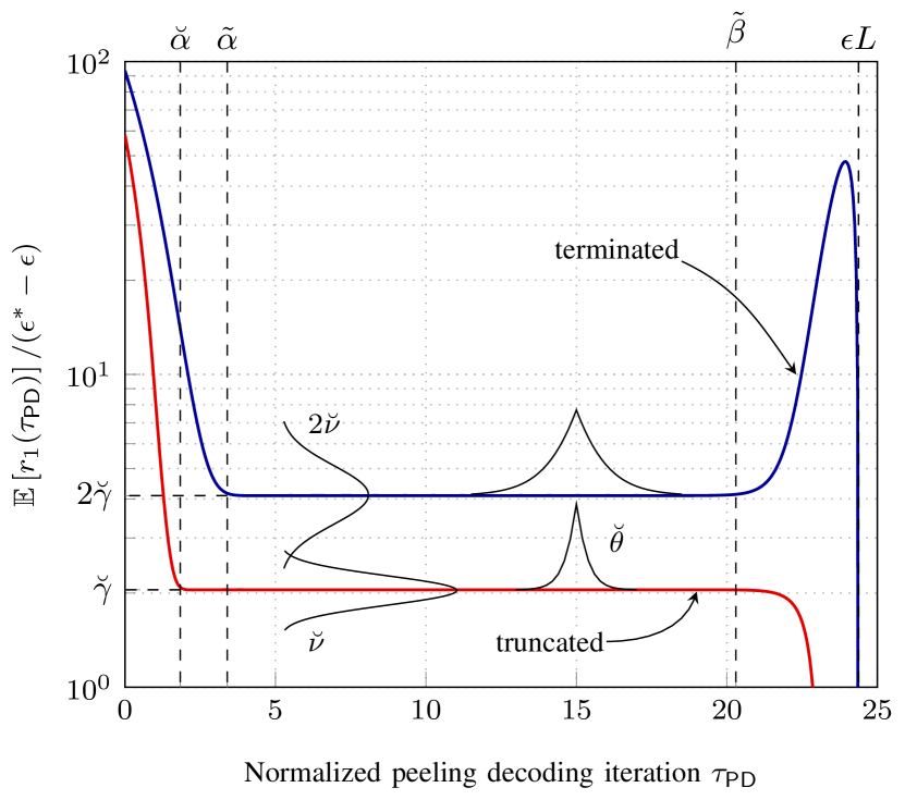
For a fixed , the distribution of converges to a Gaussian as and concentrates around its mean with expectation taken over the ensemble, channel, and peeling decoding realizations [12, 11]. The evolution of over can be obtained by numerically solving a system of coupled differential equations called mean evolution. Mean evolution equations for the semi-structured SC-LDPC code ensemble are provided in [11]. For illustration, Fig. 2 shows the mean evolution curves normalized by for the terminated (blue curve) and truncated (red curve) SC-LDPC code ensemble at .
Notably, exhibits a steady-state phase where it remains essentially constant [11]. We denote the range of corresponding to the steady state of the terminated ensemble as . Here and in the following, we denote the variables associated with the terminated ensemble with a tilde, e.g., , and those associated with the truncated ensemble with a breve, e.g., —the two “extrema” in a tilde allude to the presence of two decoding waves in the terminated ensemble, and a single “extremum” in a breve to a single wave in the truncated ensemble.
During the steady state, the two waves propagating in the terminated chain are each equivalent to the single wave present in the truncated chain. In [15], we proposed to isolate a single wave by focusing on the truncated chain and modeling the first two moments of in the same way as is done for the terminated chain in [11], namely
| (6) | ||||
| (7) | ||||
| (8) |
for a triple of real positive numbers .
Apart from the BP decoding threshold , the scaling law for unlimited number of BP iterations requires the five parameters . The first three can be estimated by numerically solving mean evolution equations. We estimate them for several and linearly interpolate the values in between. The last two can be estimated by solving an augmented system of differential equations called covariance evolution [11]. Instead, we estimate from a set of realizations of for a fixed and treat them as parameters that depend on only. The meaning of the scaling parameters for peeling decoding is illustrated in Fig. 2.
The key idea behind the scaling laws in [11, 15] is to model in the steady state by an Ornstein-Uhlenbeck process, parametrized to match the first two moments of (6)–(8). Olmos and Urbanke model the steady state of the terminated ensemble by a single Ornstein-Uhlenbeck process [11]; we proposed instead a refined model that relies on two independent Ornstein-Uhlenbeck processes and yields more accurate predictions [15]. We summarize the model in [15] here and use it as the starting point for our analysis of decoding with a limited number of iterations.
To estimate the FER, we consider the normalized time of peeling decoding at which the number of degree-one CNs—and hence the value of —drops to zero, referred to as the first-hit time ,
| (9) |
For the terminated ensemble, to exhaust all available degree-one CNs, the peeling decoder must run out of them in both the left and right decoding wave. Accordingly, we model as the sum of two independent variables and that correspond to the first-hit time of the left and right wave, respectively [15], as
| (10) |
The number of degree-one CNs available to each wave is modeled as an independent Ornstein-Uhlenbeck process. It is known that the first-hit time distribution for an Ornstein-Uhlenbeck process converges to an exponential distribution with mean as [11],
| (11) |
where and
| (12) |
The PDF of the number of degree-one CNs recovered by the left and right wave during the steady state is
| (13) |
Let denote successful decoding. Since the total number of degree-one CNs that must be recovered during the steady state of the terminated ensemble is , the probability of successful decoding can be expressed as
| (14) | ||||
In a similar manner, the FER of an unterminated SC-LDPC code ensemble evaluated over spatial positions is approximated in [15] as
| (16) |
which is the same approximation used by Olmos and Urbanke for the terminated ensemble, but with the scaling parameters estimated from the truncated ensemble instead of from the terminated ensemble.
The scaling law for the unterminated ensemble is used here and in [15] in the analysis of sliding window decoding, where the sliding window does not allow the right wave to propagate to the left by further than positions, effectively limiting the first positions to decoding by a single wave only. As we showed in [15], this results in a “two-phase” decoding, where the first phase comprises the first positions and includes a single decoding wave from the left, and the second phase comprises the last positions and may contain both the wave from the left and the wave from the right. The FER in the case of sliding window decoding with unlimited number of BP iterations can then be approximated as [15]
| (17) |
Lastly, we will use the speed of a decoding wave in our analysis. Specifically, we assume that a wave traverses positions in peeling decoding iterations. We estimate from the average number of erased VNs in the middle of the coupled chain during the steady state as
| (18) |
where , the average number of erased VNs at position at normalized iteration , is produced alongside by numerically solving mean evolution [15].
III The Speed of the Decoding Waves and the Duration of the Steady State
Besides providing BP thresholds for SC-LDPC code ensembles, density evolution, described in Section II-A, can be used to answer the following questions: How many BP iterations are needed before the steady state begins and the decoding waves establish? How fast do decoding waves propagate under BP decoding? How many iterations does it take for the decoding waves to collapse once they meet at the end of the steady state?
Let be the fraction of code bits at position recovered in BP iteration . The expected value of can be obtained from the decrease in the erasure probability across iterations of density evolution as
| (19) |
with from (4). Define . The number of code bits recovered in iteration is then , with , where
| (20) |
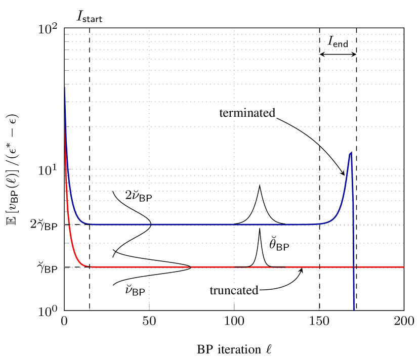
The evolution of through BP iterations is shown in Fig. 3 for the terminated (blue curve) and truncated (red curve) SC-LDPC code ensemble at . In contrast to the mean evolution curves (Fig. 2), the onset of the steady state happens at the same time for the truncated and terminated ensemble because BP decoding resolves all code bits corresponding to VNs connected to degree-one CNs in parallel.
Denote the speed of the decoding waves under BP decoding by , measured in positions traveled by the wave per BP iteration, the number of BP iterations before the onset of the decoding waves by , and the number of BP iterations it takes for the waves to collapse once they meet by . The parameters and are illustrated in Fig. 3. We estimate by tracking the mid-point of the wave fronts of over density evolution iterations, and by tracking the second difference of across iterations and comparing it with a numerical threshold (the value of is used; the average change in the erasure probability is normalized by the distance to the BP threshold prior to the comparison with the threshold). All these parameters are estimated for several values of . Linear interpolation is used to estimate the intermediate values. A similar procedure was used in [15] to estimate for peeling decoding.
As introduced in Section II, we denote the limit on the total number of BP iterations by . For decoding to be successful, the decoding waves must meet before the effective deadline of
| (21) |
iterations of BP decoding after the beginning of the steady state phase.
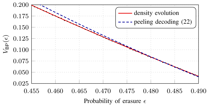
Fig. 4 shows the speed of the decoding waves during the steady state of BP decoding estimated from density evolution as a function of , . The black dots represent the values estimated directly, and the red solid line is a quadratic fit to these data.
There is an alternative way to estimate . Since a single iteration of BP decoding recovers all VNs connected to degree-one CNs, we assume that a single BP iteration during the steady state is equivalent to as many peeling decoding iterations as there are degree-one CNs available for each of the waves. This assumption allows us to approximate as
| (22) |
where is the speed of the waves under peeling decoding, which can be calculated as shown in (18), and is the average number of degree-one CNs available to one decoding wave during the steady state of peeling decoding (see (6)).
The approximation (22) is also shown in Fig. 4 (blue dashed). The good match between the direct density evolution-based estimation of (red) and the approximation in (22) (blue dashed) indicates that the number of degree-one CNs available to a decoding wave can be used as a crucial bridge between the steady-state behavior of peeling decoding and BP decoding.
IV Finite-Length Scaling: Constant
Propagation Model
For a limited number of BP iterations, the probability of successful decoding (14) should be rewritten as
| (23) |
Density evolution shows that the decoding waves propagate throughout the chain with a constant speed in the limit of . A natural first step toward a finite-length scaling law would be to also assume a constant propagation speed in the context of a finite —i.e., to assume that with every BP iteration each wave travels by exactly positions.
To understand why a limit on the number of iterations affects the probability of successful decoding, consider the following scenario: imagine one of the waves fails immediately at the beginning of the chain; imagine further that is too small for the other wave to propagate through the whole chain and meet the first wave within iterations. In that case decoding would fail even though it could have been successful without a limit on .

Our approach is to incorporate a limit on the number of BP iterations into the scaling laws for peeling decoding—analyzing BP decoding directly proves to be challenging. First, we need to account for the width of the decoding waves under peeling decoding. It takes normalized peeling decoding iterations for the waves to propagate through the chain with a constant speed of positions per normalized peeling decoding iteration (see Fig. 2). This means that the length (in positions) covered during the steady state is
| (24) |
We schematically illustrate the meaning of , which can be thought of as the effective length of the chain, in Fig. 5.
How much of that effective length should a wave cover under a limit on the number of BP iterations? Without loss of generality, take the left decoding wave, marked by in Fig. 5. In BP iterations during the steady state, the wave can propagate by up to positions. This means that for successful decoding, wave should propagate by at least
| (25) |
positions to meet wave before the deadline, as illustrated in Fig. 5. We need to bear in mind that, mutatis mutandis, the same logic applies to both the first and second wave, hence both waves need to propagate by at least positions for decoding to be successful.
Fig. 6 shows an example of calculated using (25). We observe that is zero up to a certain value of and then increases with increasing . means that a single decoding wave has enough time to propagate all the way along the chain (i.e., successful decoding is possible even if the other wave fails immediately after the onset of the steady state), so the limit on the number of iterations does not change the probability of decoding error compared to the case of unlimited number of iterations. For large , may exceed , which is when the waves do not get a chance to meet in time at all and decoding is bound to fail.
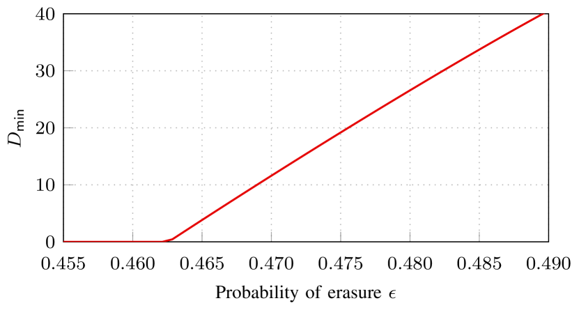
We can now use to translate the limitation on the number of BP iterations into the language of the first-hit times and . To require a wave to travel by at least positions is to ask it to survive for at least peeling decoding iterations. Bearing in mind that both waves need to survive that long to meet the deadline, we can rewrite the second condition in (23) as
| (26) |
Since the first-hit times and are exponentially distributed (11), the two conditions in (23) can be combined as
| (27) | ||||
where we assumed ; otherwise, .
The FER can therefore be estimated as
| (28) |
if and otherwise.
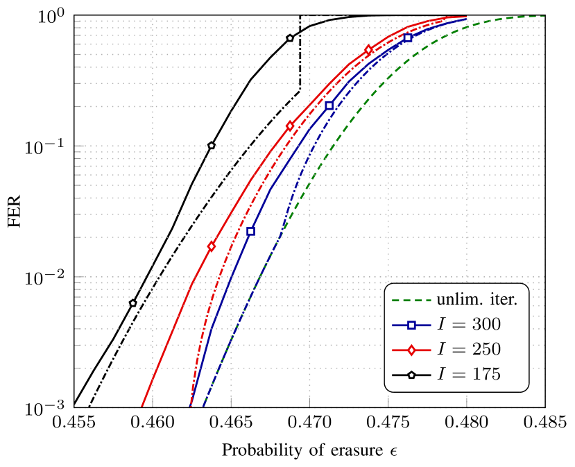
Fig. 7 compares the simulated FERs (solid curves) for the terminated SC-LDPC code ensemble with the approximation (28) (dash-dotted curves) under different limits on the number of BP iterations . Naturally, as the limit increases, the solid curves approach the FER curve for the unlimited iterations (green dashed) calculated using (15). The scaling law (28) is a reasonably accurate approximation to the simulated FER, especially given that the only change to the scaling law for unlimited iterations (15) is the introduction of the additional term in (28). However, the analytical approximation does not capture the simulated FER behavior in the regions where is either close to zero (where the approximation curve joins the green dashed curve, as for at around ) or to (where there may be a discontinuous jump to , as for at around ).
V Finite-Length Scaling: Randomized Propagation Distance Models
In this section, we introduce three scaling laws that drop the assumption that a decoding wave propagates by the same distance in every BP iteration. Indeed, the partial mismatch of the scaling law (28) to the simulated FER curves in Fig. 7 suggests that the assumption of constant wave propagation does not hold in practice for a finite number of iterations—when is sufficient for the limitation on the number of iterations not to matter for the scaling law (i.e., when predicted FER curves merge with that for full BP decoding), the waves may still fail to meet before the deadline. Likewise, when becomes so low that the law predicts the FER to be equal to one, the waves may still succeed.
Let us denote by the number of normalized peeling decoding iterations (and hence the number of VNs recovered) that corresponds to BP iterations for a decoding wave that has not run out of degree-one CNs. The scaling law in Section IV and the conversion between and in (22) effectively assume to be constant and equal to . In this section, we treat as a random variable instead.
A decoding wave stops either because it runs out of degree-one CNs or because it reaches the limit on the number of BP iterations, whichever event happens first. Correspondingly, let and denote the number of VNs recovered by the first and second wave by that time,
| (29) | ||||
where and are the first-hit times of the first and second wave, respectively, and the superscripts to emphasize that these are two independent random variables that correspond to the two decoding waves. (The two waves are numbered left to right as shown in Fig. 5.) The probability of a successful decoding can then be rewritten as
| (30) |
Essentially, the model (30) incorporates the second requirement in (23)—that there should be enough BP iterations for the two waves to meet—into and via a random variable , as opposed to incorporating it via a constant boundary as in (27).
Assuming and to be independent and to be exponentially distributed (see (11)), we approximate the PDF of as
| (31) |
where and denote the PDF and the CDF of , respectively. The same logic applies to the second wave, so the PDF of is also . We can now use (31) to estimate the FER similarly to (14) as
| (32) |
In summary, we need to approximate the distribution of and use it in (31)–(32) to predict the FER. We provide several ways to model below.
V-A Simulating Using an Ornstein-Uhlenbeck Process
We can approximate the distribution of using the following heuristic: We keep the assumption that an iteration of BP corresponds to as many iterations of peeling decoding as there are degree-one CNs available to decode. However, we no longer assume the normalized number of available degree-one CNs across iterations during the steady state, , to be constant. Instead, we assume that each BP iteration is equivalent to advancing along a peeling decoding trajectory—i.e., a realization of —by as much as there are degree-one CNs in the current position on the peeling decoding trajectory. This heuristic model allows us to directly simulate the PDF of from Monte-Carlo realizations of the Ornstein-Uhlenbeck process that correspond to realizations of the steady-state of . Indeed, from each Ornstein-Uhlenbeck realization of we can generate a realization of as
| (33) |
starting with . We remark that when is set to be constant and equal to from (6), boils back down to .
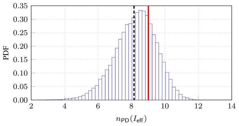
Fig. 8 shows an example PDF of simulated via (33) from Monte-Carlo realizations of the Ornstein-Uhlenbeck process with parameters in (6)–(8) chosen to match the first two moments of (blue histogram). We observe that the average value of (vertical black dashed line) is smaller than (vertical red solid line). Further, the left tail of the PDF is “heavier” than the right. This can be explained by the asymmetry in the way temporal correlation in influences in (33): when is large, will end up far away from , so the next increment in will be statistically close to a sample from an independent Gaussian random variable centered at . When is small, on the other hand, the next increment in will also likely be small.
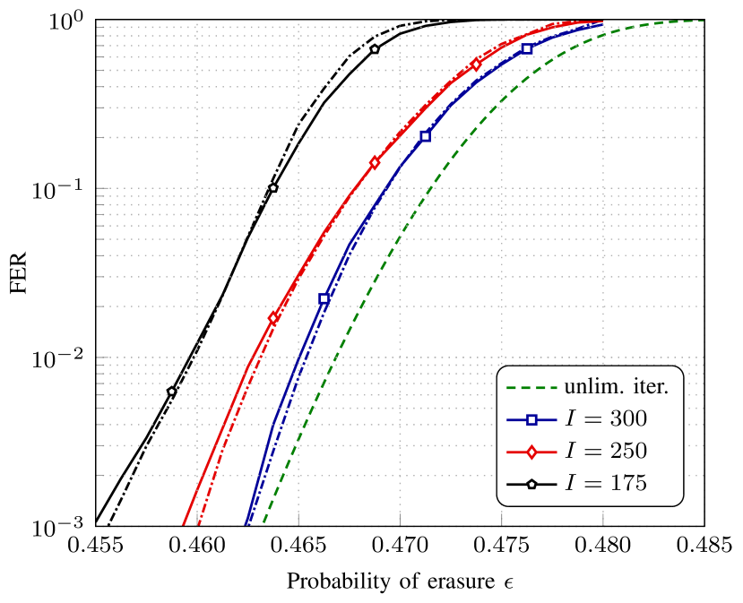
The first scaling law we propose in this section uses the simulated distribution of based on the Ornstein-Uhlenbeck model (33) in (31)–(32) to estimate the FER. The corresponding approximations are shown in Fig. 9 for the terminated SC-LDPC code ensemble and (dash-dotted curves). The match between the predicted and simulated (solid) FER curves is remarkable—evidently, the iterative model based on the Ornstein-Uhlenbeck process (33) is a good approximation of the behavior of BP decoding. The drawback of the model is that it requires Monte-Carlo approximation of the PDF of for every combination of ; however, simulating via (33) is still far less computationally complex than simulating BP decoding.
V-B Gaussian Propagation Distance Model
In this section, we introduce a model that does not require Monte-Carlo simulation of the distribution of as in Section V-A. Instead, the model approximates by a Gaussian random variable. To that end, we will rely on the fact that a time integral of an Ornstein-Uhlenbeck process is normally distributed, as we describe below.
V-B1 Ornstein-Uhlenbeck process: necessary background
A generic Ornstein-Uhlenbeck process can be described using the following stochastic differential equation:
| (34) |
where is the standard Wiener process, and are real positive constants, and is real. The first term on the right-hand side of (34) can be conceptualized as a mean-reverting factor and the second term as a random fluctuation. The constants and determine their relative importance.
For a fixed sufficiently large , the distribution of is Gaussian. Specifically,
| (35) |
Moreover, for sufficiently large ,
| (36) |
Crucially, Ornstein and Uhlenbeck showed that a time-integrated Ornstein-Uhlenbeck process is a Gaussian random variable [21]. For ,
| (37) |
This result is the cornerstone of our approximation of as a Gaussian random variable.
V-B2 Ornstein-Uhlenbeck process as a model for BP decoding
Let denote the number of new VNs (normalized by ) resolved in BP iteration , where is
| (38) |
The quantity can be interpreted as the instantaneous decoding speed, measured in VNs (normalized by ) per BP iteration. Here, the time variable is normalized by the distance to the BP threshold instead of by as is the case for , discussed in Section II-C. Up to the normalization of time, is equivalent to introduced in Section III. We use different time variables in these two cases to avoid confusion.
The process was introduced in [22] to provide an alternative finite-length scaling law for SC-LDPC code ensembles that provides less accurate predictions of the FER than the law in [15] (and even than the law in [11]) but does not rely on peeling decoding or mean evolution. Indeed, as opposed to , can be obtained directly from density evolution, as we discuss in Section III (see (20)). The authors show that exhibits a steady-state phase; they approximate the first two moments of this process during the steady-state phase as
| (39) | ||||
| (40) | ||||
| (41) |
We apply the same refinement of the law as we did in [15] and model the two-wave process for the terminated ensemble as a combination of two independent Ornstein-Uhlenbeck processes. We therefore estimate the triple from the truncated ensemble, as we did in [15] for peeling decoding to estimate . (We review the peeling decoding-based laws in Section II-C.) The steady-state level constant is estimated along with and from density evolution: once and are estimated as described in Section III, we estimate from the average of for . The covariance parameters and are estimated from Monte-Carlo simulations of BP decoding. For our running example of the SC-LDPC code ensemble, and are estimated for to be . The scaling parameters , and are illustrated in Fig. 3 along with and .
V-B3 Normal approximation based on a time-integrated Ornstein-Uhlenbeck process
The total number of VNs decoded in iterations, , can be expressed as a time integral of , divided by to convert the units of speed to VNs per normalized iteration,
| (43) |
where
| (44) |
We can now use the expression for a time-integrated Ornstein-Uhlenbeck process (37) with appropriately chosen parameters (42) to approximate the distribution of from (43) as
| (45) | ||||
| (46) |
where in (a) we used (42) and in (b) we used (44). Notably, the approximation (46) reveals that both mean and variance of grow linearly with . We must also remark that the approximation (46) does not account for the possibility that the underlying Ornstein-Uhlenbeck process becomes negative.
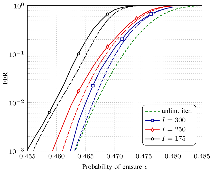
The second scaling law we propose in this section uses the normal approximation (46) to the distribution of in (31)–(32) to estimate the FER. The corresponding predictions are shown in Fig. 10 for our running example of the terminated SC-LDPC code ensemble and (dash-dotted curves). We observe that, while being a good approximation to the simulated FER, the predictions are more optimistic than the predictions based on the simulated Ornstein-Uhlenbeck process from Section V-A (cf. Fig. 9).
V-B4 Shifted normal approximation
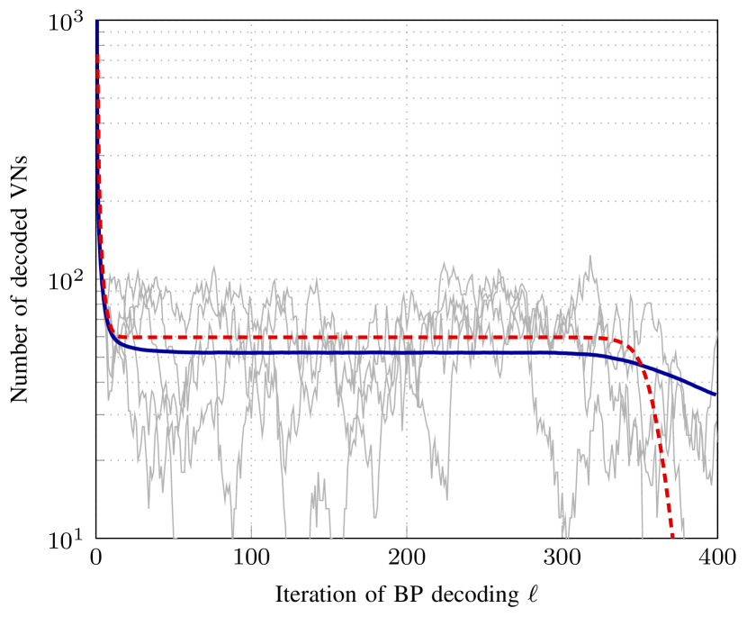
Part of the reason behind the mismatch between the simulated and predicted FER in Fig. 10 is that (39) overestimates the average number of VNs decoded in a BP iteration for finite , as shown in Fig. 11 for the truncated SC-LDPC code ensemble and .
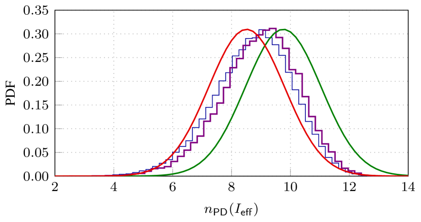
For the same ensemble and , Fig. 12 shows that the gap in the steady-state level translates into a shift in the location of the Gaussian approximation (46) to (green curve) relative to the simulated histogram (thin blue curve). Estimating the gap without resorting to Monte-Carlo simulations proves to be difficult; moreover, even if we adjust the location of the Gaussian by shifting its mean to account for the gap, the resulting distribution (red curve) lags behind the simulated histogram (thin blue curve). Overall, the simulated PDF based on the iterative Ornstein-Uhlenbeck model in Section V-A (purple curve) is the most accurate. On the other hand, the figure suggests that the two Gaussian models capture the variance of rather well.
With that in mind, we propose a hybrid model where the Gaussian approximation (46) is shifted to be located at the average of the iterative Ornstein-Uhlenbeck model (33). Specifically, let denote that average. Unfortunately, obtaining analytically is challenging; we resort to Monte-Carlo simulations of the iterative Ornstein-Uhlenbeck model (33) to estimate it. These simulations indicate that depends linearly on —we can thus estimate the slope of as for a specific and obtain the values of for other by scaling that mother curve as , thereby avoiding the need to re-simulate for every . This is equivalent to using
| (47) |
instead of in (42).
Putting it all together, the third and last scaling law we propose in this section approximates the distribution of as
| (48) |
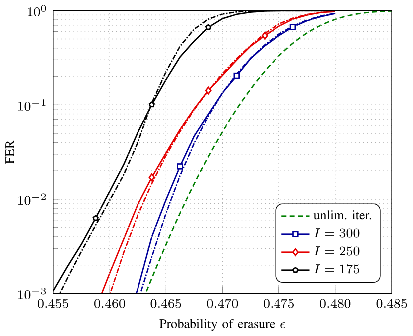
The resulting FER predictions for the SC-LDPC code ensemble are shown in Fig. 13 for (dash-dotted curves). We chose , estimated for several , and linearly interpolated it to obtain the intermediate values. (We remark that and depend on in their turn; as we discuss in Section III, we also estimate them for several and use linear interpolation to obtain the intermediate values.) The resulting predictions are very close to those in Fig. 9 by the iterative Ornstein-Uhlenbeck model (i.e., by the first scaling law proposed in this section).
We conclude that the hybrid model provides an interesting trade-off between accuracy and analytical tractability. Importantly, unlike the first scaling law in this section, it does not require Monte-Carlo simulation for every combination of —estimating from a single value of the number of BP iterations allows us to obtain the whole family of FER curves for different limits on the number of BP iterations.
V-C Discussion
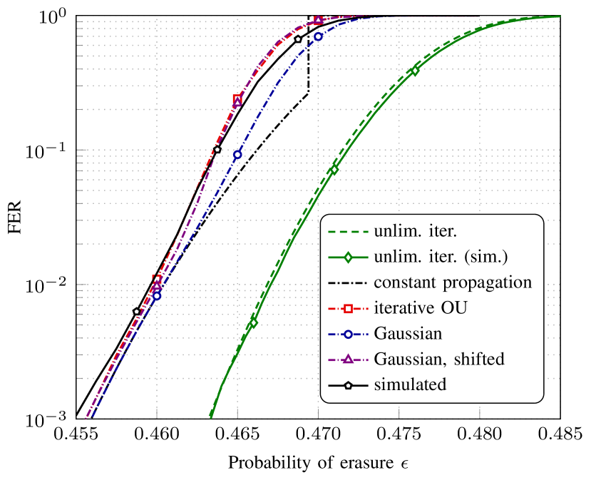
Before we tackle the FER prediction for sliding window decoding with a limit on the number of iterations in Section VI, let us summarize the performance-complexity trade-offs associated with the four scaling laws we proposed for full BP decoding. To that end, Fig. 14 groups the simulated (black solid curve with pentagons) and predicted FER curves for the terminated SC-LDPC code ensemble under full BP decoding with using the constant propagation model (28) (black dash-dotted curve) and the randomized propagation model (31)–(32) with the approximated distribution of based on the iterative Ornstein-Uhlenbeck model (33) (red dash-dotted curve with squares), on the normal distribution for the integrated Ornstein-Uhlenbeck process (46) (blue dash-dotted curve with circles), and on the shifted normal distribution (48) (purple dash-dotted curve with triangles). For reference, we have also included the simulated FER curve for unlimited number of iterations (green solid curve with diamonds) alongside our prediction from [15] (given in (15)) (green dashed curve).
Besides the scaling parameters also required for the scaling law with unlimited iterations (15), the black dash-dotted prediction curve obtained via the constant propagation model (28) requires calculating , which is a function of quantities we estimate from mean and density evolution, as we describe in Section IV. In that sense, the constant propagation model (28) is no more computationally challenging than the scaling law for unlimited iterations (15). On the other hand, the constant propagation model does not capture well the transition regions of the FER curve, as exemplified by the discontinuous jump of the black dash-dotted curve around and discussed in Section IV.
The iterative Ornstein-Uhlenbeck model (33) yields very accurate FER predictions (red dash-dotted curve with squares); however, it requires Monte-Carlo simulation of the Ornstein-Uhlenbeck process and numerical approximation of the PDF of from the simulated realizations for every . The normal approximation based on the time-integrated Ornstein-Uhlenbeck process (46), shown in Fig. 14 as the blue dash-dotted curve with circles, is computationally less complex than the iterative Ornstein-Uhlenbeck model once the parameters are estimated, since it does not require estimating a probability distribution via Monte-Carlo simulation. However, it is also less accurate. The accuracy can be improved by shifting the Gaussian to be located at the mean of the iterative Ornstein-Uhlenbeck model, which we describe in Section V-B4 to obtain the purple dash-dotted curve with triangles in Fig. 14 via (48). The shifted normal approximation is less computationally complex than the iterative Ornstein-Uhlenbeck model—not only does it rely on Gaussian distribution and thus simplify numerical integration in (32), but it also avoids simulating the iterative Ornstein-Uhlenbeck model (33) for every —while achieving similar accuracy.
VI Finite-Length Scaling: Sliding Window Decoding with a Limited Number of Iterations
The core idea behind the scaling laws in Section V is to model the number of bits recovered by a given number of BP iterations as a time integral of the Ornstein-Uhlenbeck process . In this section, we further develop this approach and use it to estimate the FER under sliding window decoding. First, however, we need to consider the specific ways in which a limit on the number of iterations affects the probability of decoding error, which we discuss in the two following subsections.
VI-A Competition Between the Left Wave and the Sliding Window
In addition to the potential failure of the decoding waves that we analyzed in [15], a limit on the number of BP iterations in sliding window decoding introduces a kind of race between the left decoding wave and the sliding window. Let denote the position of the leftmost VN that remains unrecovered by iteration . We will refer to as the position of the left wave at iteration . Analogously, let denote the leftmost position within the sliding window, and the next position just outside the right boundary of the sliding window. If, at any iteration , the left boundary of the window overtakes the wave, decoding fails, even though it could potentially have succeeded had the number of iterations not been limited. Let denote this overtaking event,
| (49) |
A necessary condition for successful decoding is that does not happen.
The setup we are considering can be illustrated by means of the following analogy. Suppose a user is watching a video via a streaming service. The video is downloading at a rate that fluctuates around a certain average. After an initial buffering period, the device starts playing the video. Then the event in question is that the buffer is exhausted (and thus the video frozen) at least once during playback.
VI-B Reduced Maximum Propagation Distance for the Right Wave
Apart from the possibility of the window overtaking the left wave, the limit on the number of iterations also affects decoding by reducing the maximum distance that can be possibly traveled by the right wave (once the sliding window reaches the right boundary of the chain). When the number of decoding iterations is not limited, we assume that the right wave can travel by up to positions, which is reflected in our scaling law for sliding window decoding (17) proposed in [15]. Here, we account for the presence of a limit on the number of iterations by estimating the maximum number of positions the right wave can travel to the left while the sliding window is moving to the right, which we denote by .
We assume the following three-phase process: In the first phase, which begins when the sliding window starts to cover the last VN position (i.e., the right boundary of the window has reached the end of the coupled chain) and lasts iterations, the right wave forms. Then, in the second phase, the right wave and the window move toward each other. Finally, in the third phase, which lasts iterations, the two decoding waves meet and collapse. During the first and third phase the right wave does not travel, whereas the window moves to the right with speed . During the second phase, the right wave travels leftward with speed , and the window moves rightward with speed . The maximum number of positions the right wave can travel, , corresponds to the distance covered by the right wave in the second phase.
During the first and third phase, the window slides by
| (50) |
positions while the right wave does not move. The remaining
| (51) |
positions will be covered by the window and the wave jointly with speed , which will take
| (52) |
iterations. During that time, the right wave will have traveled by
| (53) |
positions, which is the adjusted size of the sliding window we use in our model below. Naturally, as the limit on the number of iterations is relaxed, in (53) and therefore .
VI-C General Form of the Scaling Law
We incorporate the limit on the number of iterations during sliding window decoding into our model via the two effects outlined above, namely, the possibility that the window overtakes the left wave (an event denoted by ) and the reduction of the maximum distance the right wave can travel. In essence, successful decoding requires that (i) the overtaking does not happen; (ii) the left wave does not run out of VNs to decode while propagating through the first positions; and (iii) the left and right wave jointly cover the last positions. Conditions (ii) and (iii) are equivalent to the two-phase model we proposed in [15] to estimate the FER under unlimited iterations as in (17); the only adjustment is that the size of the second phase is reduced from to , defined in (53), to account for the reduction of the maximum reach of the right wave, as discussed in more detail in Section VI-B. Condition (i) is introduced in Section VI-A.
Modeling the three conditions as independent events, we approximate the FER under sliding window decoding with a limit on the number of BP iterations as
| (54) |
where and are the estimated FERs for the unterminated and terminated SC-LDPC code ensembles of length and , and are defined in (15) and (16), respectively.
The rest of the section is devoted to the estimation of , the core of our finite-length scaling law for sliding window decoding with a limited number of iterations.
VI-D Modeling the Race Between the Left Wave and the Window
The general idea behind our approach is to model the stochastic process associated with the position of the left wave, , by a scaled time integral of the Ornstein-Uhlenbeck process that corresponds to , the normalized number of bits recovered in iteration defined in Section III, with an additional noise term. The wave cannot overtake the right boundary of the window, , because no BP iterations are performed there. On the other hand, if the wave is itself overtaken by the left boundary, , decoding is bound to fail. This motivates us to incorporate the boundaries of the window into our model as an absorbing barrier at and a reflecting barrier at . When a stochastic process hits an absorbing barrier, it remains absorbed indefinitely. When a stochastic process hits a reflecting barrier, it is reflected back inside the domain [23]. The overtaking event that we introduced in Section VI-A in (49) corresponds to having been absorbed by iteration . The probability of this event can be estimated by tracking the evolution of the PDF of across iterations. That evolution can in turn be described by a partial differential equation called the Fokker-Planck equation [23]. We numerically solve the initial value problem for the Fokker-Planck equation for with the boundary conditions that correspond to an absorbing barrier at and a reflecting barrier at and obtain the estimation of the probability of .
VI-D1 Position of the left wave as an integrated Ornstein-Uhlenbeck process
The scaling law for full BP decoding proposed in Section V uses a time integral of the Ornstein-Uhlenbeck process as a model for the total number of VNs (normalized by ) decoded in a given number of BP iterations. In the context of sliding window decoding, we are interested instead in the position of the wave after a number of iterations. The basic element of our model is the conversion of the normalized number of VNs decoded in BP iteration , , to the number of positions traveled by the wave in that iteration. We assume that VNs decoded during the steady state of BP decoding advance the wave by positions—i.e., by the same number of positions as for peeling decoding (18). The number of positions traveled in iteration is then
| (55) |
and the total number of positions traveled in steady-state BP iterations is
| (56) |
where is number of VNs decoded in steady-state BP iterations that we introduced in Section V. We can use the model (43) of in (56) to obtain
| (57) |
For convenience, we have assumed here that iteration corresponds to the beginning of the steady state when the position of the wave is zero.
To declutter notation, we do not use the time normalized by the distance to the threshold (38) as we do in Section V and in (57). Instead, we use a continuous version of the variable with a unit of time also measured in BP iterations, denoted by . The model (57) can be rewritten in terms of as
| (58) |
As we do for in Section V-B2, we model by an Ornstein-Uhlenbeck process of the form (34). The parameters and need to be rescaled relative to those in (42), resulting in
| (59) | ||||
the two models (i.e., the one with rescaled time and the one with rescaled and ) are equivalent and yield identical predictions. We remark that in this section we use the same value for the average steady-state level of as in the shifted normal approximation (47).
The scaling law in Section V requires the probability distribution of the time integral of an Ornstein-Uhlenbeck process for a specific , which is known to be Gaussian (37). The analysis of sliding window decoding requires a more granular approach, since we need to track the evolution of over iterations. In other words, we need to treat as a stochastic process in its own right. This is complicated by the fact that an integrated Ornstein-Uhlenbeck process of the form (37) or (58) is not Markov. However, the two-dimensional process
| (60) |
is Markov and can be analyzed using standard tools for diffusion processes [23]. (A diffusion process can informally be thought of as a continuous-time Markov processes with continuous sample paths [23].) The corresponding stochastic differential equation is [24, Eq. (35)]
| (61) |
where is the standard Wiener process. To account for the scaling of the Ornstein-Uhlenbeck process (defined via (34) with parameters (59)) by in (60), and in (61) should be rescaled relative to those in (59), resulting in
| (62) | ||||
The need for a subscript in the diffusion coefficient will become apparent in the next subsection.
VI-D2 Additional diffusion of the left wave’s position
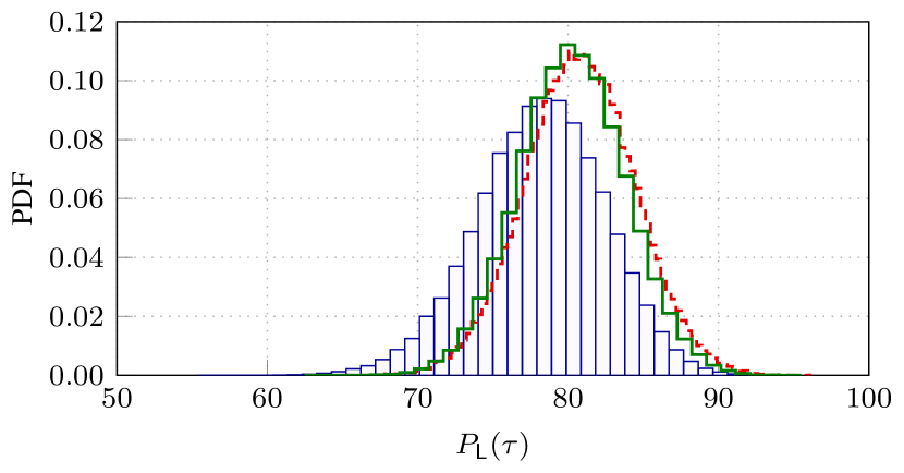
To answer whether the integrated Ornstein-Uhlenbeck process (61)–(62) is a good model for the propagation distance of the left wave, it can be tested against direct Monte-Carlo simulation of the decoding process. Fig. 15 compares the distribution of obtained via direct simulation (blue filled histogram) with the one estimated by simulating (red dashed curve) and (green solid curve) using (61)–(62). The integrated Ornstein-Uhlenbeck model captures the average position of the wave relatively well (the means of the blue and green histogram are approximately and positions, respectively, after BP iterations) but underestimates its variance. In other words, the uncertainty in the wave’s position does not come solely from the variation in the number of decoded VNs; there must be other factors at play.
We model this additional source of uncertainty via an additional diffusion term that affects directly. Throughout iterations, even if the number of decoded VNs is known, the positions of these VNs is subject to random fluctuation. As Fig. 15 shows, by time that fluctuation accumulates into a difference in variance between simulated and from the model (61)–(62). We denote the variance of the simulated by and that of from (61)–(62) by . We introduce a parameter that corresponds to additional per-iteration variance in position,
| (63) |
and incorporate that additional source of variance into our model by changing (61) to
| (64) |
where is another standard Wiener process independent of . The rationale behind this model is that the variance of the standard Wiener process grows linearly with time [23]; adding the term in (64) results in an additional variance of in compared with the model in (61), thereby canceling the mismatch between the simulated and the modeled variance in (63) but “spreading” this variance evenly across iterations.
We treat as a scaling parameter that depends on only. We rely on a set of simulated realizations of the decoding process for a certain triple to estimate . For our running example of the SC-LDPC code ensemble, we use and obtain .
As an aside, we remark that the video streaming analogy we introduced in Section VI-A can be stretched further to include the additional uncertainty we are modeling here. Indeed, the amount of downloaded data is not the only factor that determines how much time of playback is gained. This is also affected by, e.g., how much movement occurs in consecutive frames of the video, assuming the video is compressed before transmission.
VI-D3 Modeling the boundaries of the sliding window
We are now ready to incorporate the sliding window into our model. In essence, we do so by limiting the process to the range from to , i.e., to the range of positions covered by the sliding window at iteration . Indeed, cannot be larger than because sliding window decoding does not perform any BP iterations there. Similarly, if ever becomes smaller than , the overtaking happens and decoding fails. We account for these effects in our model by introducing an absorbing barrier at and a reflecting barrier at .
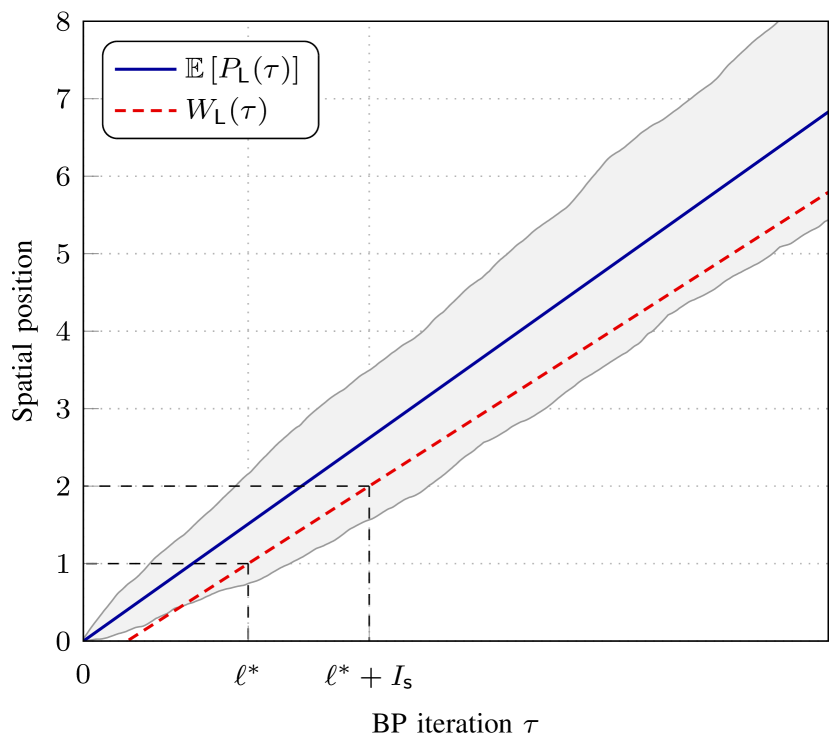
During decoding, the sliding window moves in discrete steps. It is convenient to smoothen this movement and assume it to be continuous and linear instead. We denote the continuously moving boundaries of the window by and . The setup we use is illustrated in Fig. 16. The red dashed line corresponds to , which will be included in the model as an absorbing barrier. Its slope is known and equal to . What remains to be specified is the iteration where crosses , which we denote by (see Fig. 16).
The value of is what couples the model for with . First, depends not only on but also on the time it takes for the wave to form, . A natural choice for in that regard would be : it takes iterations for the steady state to establish, which eats away from the budget of initial iterations, and then the window slides to position . However, numerical simulations show that is already around one, not zero. In our model, we would like instead to set the initial position of the wave to zero. We therefore subtract from a term that corresponds to in (62), which is the average time it takes for the wave to propagate by one position, and set
| (65) |
Using our knowledge that and that the slope of is , we obtain the continuous version of as
| (66) |
For simplicity, we ignore the fact that remains flat for the first iterations and let
| (67) |
With (66)–(67) we have ensured that the boundaries of the window, and , grow linearly with . They correspond to time-dependent absorbing and reflecting barriers and make the domain of change over time. We remove that dependency by subtracting the time-dependent term from . That corresponds to subtracting from , which can in turn be expressed as a change in .
Putting it all together, we use the model (64) with
| (68) | ||||
and the boundaries
| (69) | |||||
| (70) |
which no longer depend on . The initial conditions are as in (35) and .
The probability of the overtaking event corresponds to the probability of being absorbed at the barrier by the time . The latter probability can be obtained by solving the Fokker-Planck equation for with appropriately chosen initial and boundary conditions. The following subsection provides a summary of the associated results for general multidimensional diffusion processes.
VI-D4 Necessary background on the Fokker-Planck equation
Let be a time-homogeneous diffusion process on defined as the solution to the Itô stochastic differential equation [23, Ch. 3]
| (71) |
where is the standard Wiener process on , is a drift vector, and . The matrix is known as the diffusion matrix of . Let the initial condition be a random variable with probability density independent of . Then the probability density of is the solution to the initial value problem for the Fokker-Planck (also known as forward Kolmogorov) equation
| (72) | ||||
where and denote the components of and respectively [23, Proposition 3.3 and Eq. (4.1)]. The Fokker-Planck equation describes the evolution of the probability density of over time.
Absorbing or reflecting barriers affect through additional boundary conditions for the Fokker-Planck equation (72). An absorbing barrier imposes a Dirichlet boundary condition on (72), namely
| (73) |
Likewise, a reflecting barrier translates into a Neumann boundary condition for (72). Specifically,
| (74) |
where denotes a vector normal to . In other words, the probability density must vanish at the absorbing barrier , and there should be no probability flow at the reflecting barrier [23, pp. 90–91]. The probability mass lost by is equal to the probability of having been absorbed at by the time ,
| (75) |
assuming to be the only absorbing barrier present [23, p. 239]. The integration in performed over that denotes the domain of .
VI-D5 The Fokker-Planck equation for the proposed model
We can therefore use (72)–(74) to derive the Fokker-Planck equation for the evolution of the PDF of the process (64) as
| (77) |
with boundary conditions
| (78) | ||||
where and are defined in (69) and (70), respectively, and the parameters are given in (68) and (63).
As we specify in Section VI-D3, the initial distribution of and should be and , where . We should therefore set to a PDF whose marginal for is the PDF of and for the Dirac delta function. Handling such a distribution numerically is challenging; instead, we set to the PDF of the correlated two-dimensional Gaussian distribution
| (79) |
where and . As , the PDF of tends to the Dirac delta function as required; the correlation parameter should tend to because as , and its integral become ever more dependent. The use of the PDF of (79) allows us to avoid the aforementioned numerical issues by backing and off from their limits.
VI-D6 Numerical solution to the Fokker-Planck equation
To the best of our knowledge, the closed-form solution to the Fokker-Planck equation (77) in the presence of the boundary conditions (78) is not available. We therefore resort to solving (77)–(78) numerically using FiPy, a finite-volume solver of partial differential equations [25]. The range of is limited to to cover most of the probability mass without overstretching the domain, and that of to . The resulting rectangular domain is discretized into a regular grid with and split into and segments, respectively. We set and . The solver treats (77) as a convection-diffusion equation; we use implicit convection and diffusion terms [25], which allows us to choose a large time step without encountering numerical stability issues.
The numerical solution is propagated forward in time until the window is slid through the entire chain, i.e., until
| (80) |
The PDF is used to estimate the probability of the overtaking event according to (75) as
| (81) |
The estimated is then used in (54) to estimate the FER.
We note that our implementation of the solver takes longer to estimate the FER than direct Euler-Maruyama simulation of realizations of (64) to the same end. However, the computational complexity of the estimation based on the Fokker-Planck equation does not depend on the FER to attain a given accuracy, which is not the case for the simulation-based approach. Moreover, no attempt has been made to optimize either implementation.
VI-E Numerical Results
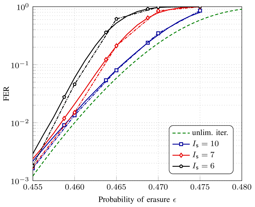
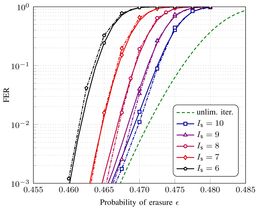
Fig. 17 compares the FER for the SC-LDPC code ensemble under sliding window decoding with and for (solid curves) with the corresponding approximation using (54), where the overtaking probability is estimated using (81) (corresponding dash-dotted curves). We observe an impressive match between the simulated and predicted error rates. A similarly accurate prediction is obtained for in Fig. 18 and for other values of with (not shown).
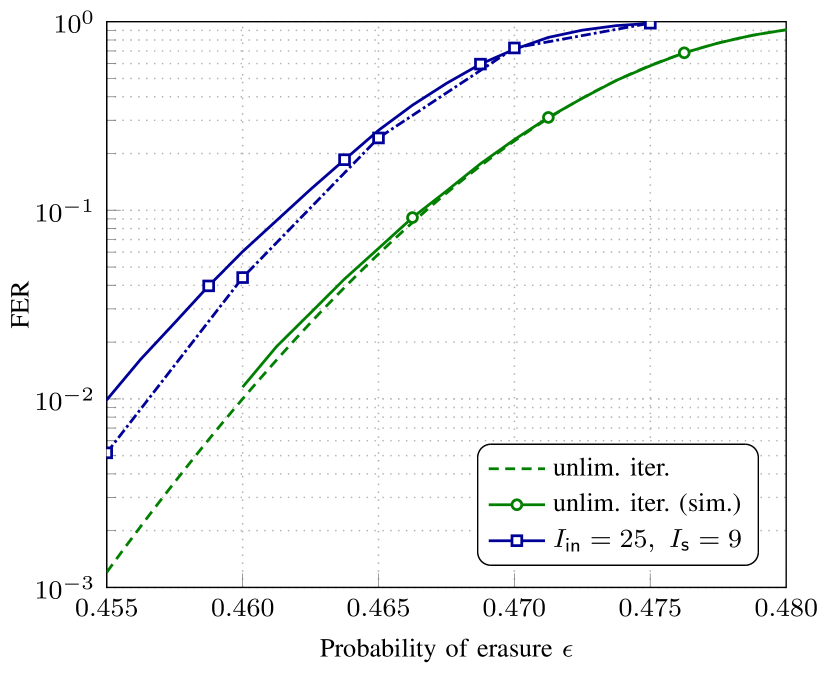
The quality of the prediction deteriorates for smaller , as exemplified in Fig. 19 for and . We observe that degradation when is such that the left wave is often overtaken at the very beginning of the chain. This setup, however, is of limited practical relevance—it is sensible for the system designer to ensure that the wave is firmly established by choosing sufficiently large. This also lowers the probability that the wave is overtaken by the window early on during decoding if wave propagation happens to slow down for some time. We have included in Fig. 19 the simulated FER curve for unlimited number of iterations (green solid curve with diamonds) alongside our prediction from [15] using (17) (green dashed curve) for reference.
We remark that we use estimated at to obtain the predictions in Figs. 17–19. This is smaller than used in Section V and estimated at . Choosing the latter value makes the prediction curves slightly more optimistic. The covariance decay parameter seems to exhibit a stronger dependency on than in the case of peeling decoding; we leave the investigation of this dependency as a subject for future work. As a general rule of thumb, one should estimate for that lie within the range they are interested in.
VII Conclusion and Discussion
The proposed scaling laws for full BP decoding with a limited number of iterations and a scaling law for sliding window decoding with a limited number of iterations provide accurate predictions of the FER. Modeling the number of bits decoded in a given number of iterations by a time integral of an Ornstein-Uhlenbeck process—the cornerstone of our scaling laws—proves to be a powerful tool in the analysis of decoding schemes with practically relevant constraints on the maximum number of iterations. More broadly, low-dimensional diffusion processes seem to be able to capture much of the behavior of iterative decoders relevant for error rate prediction.
Another takeaway is that it is important for sliding window decoding to perform a sufficient number of iterations at the beginning of the chain. It is necessary not only because the decoder must ensure that the decoding wave is established, but also because allowing the decoding wave to propagate further inside the window builds up the decoder’s resilience to variation in the wave’s propagation speed.
We also remark that the scaling laws we propose in this paper can be extended to predict the bit and block error rate using the same techniques we employed in [15] to the same end. (Block error rate refers to the probability that a spatial position—a block—contains unrecovered bits after decoding.) Specifically, the models for both full BP decoding in Sections IV–V and for sliding window decoding in Section VI already keep track of the number of bits decoded across iterations implicitly; what is required to obtain a scaling law for bit and block error rate is to make use of this knowledge and average the bit and block error rate expressions over the probability distributions of when decoding stops, which we did in [15] in the context of unlimited number of iterations.
Further, we do not foresee substantial difficulties in extending the scaling laws proposed here to protograph-based ensembles. What is required to do so is to modify density and mean evolution equations to account for the changed Tanner graph connectivity, as it is done in [13] for unlimited number of decoding iterations.
References
- [1] A. Jimenéz Feltström and K. S. Zigangirov, “Time-varying periodic convolutional codes with low-density parity-check matrix,” IEEE Trans. Inf. Theory, vol. 45, no. 6, pp. 2181–2191, Sep. 1999.
- [2] M. Lentmaier, A. Sridharan, D. J. Costello, and K. S. Zigangirov, “Iterative decoding threshold analysis for LDPC convolutional codes,” IEEE Trans. Inf. Theory, vol. 56, no. 10, pp. 5274–5289, Oct. 2010.
- [3] S. Kudekar, T. J. Richardson, and R. L. Urbanke, “Threshold saturation via spatial coupling: Why convolutional LDPC ensembles perform so well over the BEC,” IEEE Trans. Inf. Theory, vol. 57, no. 2, pp. 803–834, Feb. 2011.
- [4] S. Kudekar, T. Richardson, and R. L. Urbanke, “Spatially coupled ensembles universally achieve capacity under belief propagation,” IEEE Trans. Inf. Theory, vol. 59, no. 12, pp. 7761–7813, Dec. 2013.
- [5] A. Sridharan, D. Truhachev, M. Lentmaier, D. J. Costello, and K. S. Zigangirov, “Distance bounds for an ensemble of LDPC convolutional codes,” IEEE Trans. Inf. Theory, vol. 53, no. 12, pp. 4537–4555, Dec. 2007.
- [6] S. Moloudi, M. Lentmaier, and A. Graell i Amat, “Spatially coupled turbo-like codes,” IEEE Trans. Inf. Theory, vol. 63, no. 10, pp. 6199–6215, Oct. 2017.
- [7] B. P. Smith, A. Farhood, A. Hunt, F. R. Kschischang, and J. Lodge, “Staircase codes: FEC for 100 Gb/s OTN,” J. Lightw. Technol., vol. 30, no. 1, pp. 110–117, Jan. 2012.
- [8] V. Aref, N. Macris, R. Urbanke, and M. Vuffray, “Lossy source coding via spatially coupled LDGM ensembles,” in Proc. IEEE Int. Symp. Inf. Theory (ISIT), Cambridge, MA, Jul. 2012, pp. 373–377.
- [9] D. L. Donoho, A. Javanmard, and A. Montanari, “Information-theoretically optimal compressed sensing via spatial coupling and approximate message passing,” IEEE Trans. Inf. Theory, vol. 59, no. 11, pp. 7434–7464, Nov. 2013.
- [10] A. R. Iyengar, M. Papaleo, P. H. Siegel, J. K. Wolf, A. Vanelli-Coralli, and G. E. Corazza, “Windowed decoding of protograph-based LDPC convolutional codes over erasure channels,” IEEE Trans. Inf. Theory, vol. 58, no. 4, pp. 2303–2320, Apr. 2012.
- [11] P. M. Olmos and R. L. Urbanke, “A scaling law to predict the finite-length performance of spatially-coupled LDPC codes,” IEEE Trans. Inf. Theory, vol. 61, no. 6, pp. 3164–3184, Jun. 2015.
- [12] A. Amraoui, A. Montanari, T. Richardson, and R. Urbanke, “Finite-length scaling for iteratively decoded LDPC ensembles,” IEEE Trans. Inf. Theory, vol. 55, no. 2, pp. 473–498, Feb. 2009.
- [13] M. Stinner and P. M. Olmos, “On the waterfall performance of finite-length SC-LDPC codes constructed from protographs,” IEEE J. Sel. Areas Commun., vol. 34, no. 2, pp. 345–361, Feb. 2016.
- [14] D. J. Costello, D. G. M. Mitchell, P. M. Olmos, and M. Lentmaier, “Spatially coupled generalized LDPC codes: Introduction and overview,” in Proc. 10th IEEE Int. Symp. Turbo Codes and Iterative Inf. Process. (ISTC), Hong Kong, China, Dec. 2018.
- [15] R. Sokolovskii, A. Graell i Amat, and F. Brännström, “Finite-length scaling of spatially coupled LDPC codes under window decoding over the BEC,” IEEE Trans. Commun., vol. 68, no. 10, pp. 5988–5998, Oct. 2020.
- [16] H.-Y. Kwak, J.-W. Kim, and J.-S. No, “Optimizing code parameters of finite-length SC-LDPC codes using the scaling law,” IEEE Access, vol. 9, pp. 118 640–118 650, Aug. 2021.
- [17] R. Sokolovskii, A. Graell i Amat, and F. Brännström, “On doped SC-LDPC codes for streaming,” IEEE Commun. Lett., vol. 25, no. 7, pp. 2123–2127, Jul. 2021.
- [18] H.-Y. Kwak, J.-W. Kim, H. Park, and J.-S. No, “Optimization of SC-LDPC codes for window decoding with target window sizes,” IEEE Trans. Commun., 2022, Early Access.
- [19] M. G. Luby, M. Mitzenmacher, M. A. Shokrollahi, D. A. Spielman, and V. Stemann, “Practical loss-resilient codes,” in Proc. Annu. ACM Symp. Theory Comput. (STOC), El Paso, TX, USA, 1997, pp. 150–159.
- [20] M. G. Luby, M. Mitzenmacher, M. A. Shokrollahi, and D. A. Spielman, “Efficient erasure correcting codes,” IEEE Trans. Inf. Theory, vol. 47, no. 2, pp. 569–584, Feb. 2001.
- [21] G. E. Uhlenbeck and L. S. Ornstein, “On the theory of the brownian motion,” Phys. Rev., vol. 36, pp. 823–841, Sep. 1930.
- [22] M. Stinner, L. Barletta, and P. M. Olmos, “Finite-length scaling based on belief propagation for spatially coupled LDPC codes,” in Proc. IEEE Int. Symp. Inf. Theory (ISIT), Barcelona, Spain, Jul. 2016, pp. 2109–2113.
- [23] G. A. Pavliotis, Stochastic Processes and Applications. Springer, New York, NY, USA, 2014.
- [24] E. Benedetto, L. Sacerdote, and C. Zucca, “A first passage problem for a bivariate diffusion process: Numerical solution with an application to neuroscience when the process is Gauss-Markov,” J. Comput. Appl. Math., vol. 242, pp. 41–52, 2013.
- [25] J. E. Guyer, D. Wheeler, and J. A. Warren, “FiPy: Partial differential equations with Python,” Comput. Sci. Eng., vol. 11, no. 3, pp. 6–15, 2009. [Online]. Available: http://www.ctcms.nist.gov/fipy