Hierarchical Clustering and Matrix Completion for the Reconstruction of World Input-Output Tables

Abstract

World Input-Output (I/O) matrices provide the networks of within- and cross-country economic relations. In the context of I/O analysis, the methodology adopted by national statistical offices in data collection raises the issue of obtaining reliable data in a timely fashion and it makes the reconstruction of (part of) the I/O matrices of particular interest. In this work, we propose a method combining hierarchical clustering and Matrix Completion (MC) with a LASSO-like nuclear norm penalty, to impute missing entries of a partially unknown I/O matrix. Through simulations based on synthetic matrices we study the effectiveness of the proposed method to predict missing values from both previous years data and current data related to countries similar to the one for which current data are obscured. To show the usefulness of our method, an application based on World Input-Output Database (WIOD) tables – which are an example of industry-by-industry I/O tables – is provided. Strong similarities in structure between WIOD and other I/O tables are also found, which make the proposed approach easily generalizable to them.

1 Introduction

The world economy is characterized by the interdependence of all countries with respect to their industrial activities. It can be modeled as a network in which each “country-sector” pair exchanges goods and services with any other (and even the same) such pair, at a different extent and using different technologies. The structure of this network may provide information about such interdependencies of national economies and their changes over time. The literature usually refers to the study of these interdependencies with the term “Input-Output (I/O) analysis”. I/O tables portray flows of what is produced by some economic agents and consumed by other economics agents (either as intermediate or final consumption). They are arranged into two types, either according to relationships between industries (industry-by-industry I/O tables) or according to relationships between products (product-by-product I/O tables). Many world I/O tables for selected countries are periodically produced by, e.g., the World Input-Output Database (WIOD, Timmer2015 ; Timmer2016 ), the EORA Global Supply Chain initiative Lenzen2012 , EXIObase Tukker2013 , the Full International and Global Accounts for Research in input-Output analysis (FIGARO, Remond2019 ) from EUROSTAT, and OECD OECD2018 . By analyzing I/O matrices, McNerneyFath2013 ; Cerina2015 ; Zhu2015 studied the network topology of inter-industry flows and LiangQi2016 investigated its scaling patterns. Some studies highlighted the presence of significant asymmetry between inflow data (i.e., what a “country-sector” pair uses from other “country-sector” pairs) and outflow data (i.e., what a country-sector sells to other “country-sector” pairs), and the emergence of a clustering pattern among either countries or sectors. This can derive, e.g., from the presence of similar production technologies (i.e., similar dependence of two specific countries or sectors on other “country-sector” pairs) Carvalho2009 . This issue was taken into account, e.g., in ZhuMorrisonPuligaChessaRiccaboni2018 , where an ad-hoc measure was used to detect patterns of similarity and to group together similar countries and similar sectors, and in OlivaSetolaPanzieri2016 , where a spectral clustering approach was applied to group similar sectors of the Italian economy.

Our work has to do with the reconstruction of I/O matrices. The interest in this topic arises if one takes into account some aspects related to the methodology of data collection adopted by national statistical offices. Indeed, based on Percoco2006 , the work WenXuWen2014 provides the following motivations to apply a reconstruction method to I/O matrices:

• Data collection for I/O matrices is typically based on direct methods, e.g., on surveys ( made at different times and in different countries), which leads to classical sampling errors;

• For large surveys, errors from the inference design can easily arise;

• The elements of an I/O matrix change over time. However, collecting them in a timely fashion (for instance, once for each country every year) is an almost impossible task, due to limited resources. For this reason, historical data are typically used to approximate the current I/O matrix.

Direct compilation of I/O tables does not rely only on surveys but also on administrative registers (e.g., firms registries, accountancies of companies in official registers, public budget documents, trade customs information, taxes authorities reports, households registers), censuses (population, firms directories) and, among others, sectorial reports providing global economic information about specific sectors in an industry or in a country. It follows that, in order to compile an I/O table, many different statistical sources are contrasted (sometimes even contradictory ones). This is a huge time-consuming and resources-consuming operation, and the time gap between the publication of an I/O table and its reference year is one of the main reasons why also indirect methods exist (see Valderas-Jaramilloetal2019 for a review).

In this work, taking advantage from the similarity patterns discussed above, we apply, as an indirect method, Matrix Completion (MC, Hastie2015 ; Mazumder2010 ; Negahban2012 ) to I/O submatrices associated with suitable groups of countries, by judiciously clustering them together, via a proper clustering method. We recall here that MC is a set of advanced statistical methods that can be used to predict unobserved entries of a matrix in terms of the set of the remaining observed entries (more technical details about MC are reported later in Subsection 2.2). In this way, the partially observed matrix is “completed” by the predictions produced by MC. We show that using a selected group of similar countries permits to increase the effectiveness of MC. This is done by comparing the results obtained by MC when, on the contrary, the selected group is made by highly dissimilar countries. To the best of the authors’ knowledge, this is the first article in which MC is applied to I/O tables in connection with clustering.

The aforementioned similarity patterns have important consequences on the structure of the I/O matrices, justifying the application of MC. In fact, due the presence of countries that share similar technologies for producing the same goods, an I/O matrix might be low-rank, or, at least, might be well-approximated by a low-rank matrix (in the sense that a few singular values would dominate all the other ones, i.e., the singular values would decade quickly to $0$). This low-rank (approximation) property suggests, among other possible statistical or machine learning techniques, the adoption of MC to reconstruct potentially missing entries in an I/O matrix. Moreover, such a property is a necessary condition for obtaining good MC results (see Appendix A.1 for a discussion on this issue). Nevertheless, the application of MC to a full I/O matrix is not straightforward, since elements in different blocks of that matrix have quite different orders of magnitude. Having analyzed different real-world I/O matrices, we found that: (1) within-country values are way larger than cross-country ones; (2) I/O matrices are sparse, because of many cross-country zero entries, and (3) there is a clear separation between large-to-large countries’ values and small-to-small countries’ ones. This suggests performing a pre-processing step, in which some blocks are removed from the full I/O matrices. In particular, we focus our analysis on bilateral trade blocks, which is quite a relevant problem in multi-country and multi-regional I/O tables.

Based on cross-country subsets of real-world I/O matrices, we performed a panel analysis using MC based on a LASSO-like nuclear norm penalty Mazumder2010 ; Negahban2012 , which permits, through a suitable choice of the regularization parameter (based on a validation set), to select the number of non-zero singular values to be kept in the reconstructed matrix. The specific selection of countries was generated by the output of hierarchical clustering, whose application was based on a dissimilarity measure (the Average Absolute Correlation Distance or AACD, see later) highly related to the successive application of MC. Robustness of the results produced by hierarchical clustering was evaluated by considering synthetic counterparts of real-world I/O matrices, presenting a structure that is common to many I/O tables. This was done in order to generalize the approach to all kinds of I/O matrices, not limiting just to only one of them.

In summary, this paper proposes a two-step methodological approach where, in the first step, judiciously selected groups of countries – in terms of either i) the distribution by country-industry from where they buy inputs, or ii) the distribution by country-industry to which they sell outputs – are retrieved using a hierarchical cluster analysis Revelle1979 . This choice is preferable to other clustering techniques (e.g., $k$-means clustering MacQueen1967 ) to group countries according to their I/O exchanges where the set of countries themselves is not a-priori partitioned into a certain number of groups, but their complex structure suggests a hierarchy of clusters (see also Subsection 2.2 for other technical motivations behind this choice). In the second step, an I/O submatrix associated with this selection of countries is analysed based on a LASSO-like algorithm for MC. In particular, our approach is applied to a 5-year panel of (cross-country subsets of) I/O matrices for subsets of countries selected after performing hierarchical clustering, where a known part of the matrix associated with a specific year (i.e., the latest one) has been artificially obscured. The validation/testing phase is based on the Root Mean Square Error (RMSE) and on the Symmetric Mean Absolute Percentage Error (SMAPE) between actual and estimated values of the obscured part of the matrix, which is not provided as input to the MC algorithm. Ad-hoc simulations have been also performed in order to i) evaluate the improvement that could be achieved by a suitable pre-processing of raw data (by eliminating domestic blocks); ii) select the proper number of clusters; iii) evaluate the MC performance if the clustering failed in the first step. According to the latter point, we apply MC to subsets of either similar (cluster does not fail) or dissimilar (cluster fails) countries.

Results show the effectiveness of the proposed method to predict missing values in the current I/O matrix from both previous years data and current data related to countries similar to the one for which current data are obscured. In contrast, the effectiveness reduces, as expected, if similar countries are replaced by ones belonging to quite different clusters.

The rest of the manuscript begins with presenting the proposed methodological approach in Section 2 and reports the specific application to WIOD and simulated matrices and its results in Section 3. Section 4 is dedicated to future research directions and conclusions. To improve the readability of the work, some details (especially related to Section 3) are deferred to footnotes and to the Appendix.

2 Methods

2.1 The Input-Output model

The traditional I/O matrix Leontief1986 depicts inter-industry relationships within an economy (or country), showing how the output from one sector becomes an input to another sector ( or itself), or it contributes to the final demand. Row indices represent inputs (in nominal monetary values) from an industrial sector, while column indices represent intermediate outputs to a given sector or needed to produce a final output. This kind of table shows how dependent each sector is on every other sector, both as a customer of outputs from other sectors, and as a supplier of inputs.

Suppose an economy with $n$ sectors and $l$ final outputs is given, the assumption of constant returns to scale can be made, and sectors use inputs in fixed proportions. Fix also a specific year. In that year, each sector $i$ produces a monetary value $x_{i}$ of good $i$. Let $z_{i,j}$ be the value that sector $i$ sells to sector $j$ in that year, and let $f_{i,j}$ be the value that sector $i$ sells to the final user in that year, to produce the final output $j$. In matrix notation, if one lets

$$\mathbb{x}=\begin{bmatrix}x_{1}\\ \cdot\\ \cdot\\ \cdot\\ x_{n}\end{bmatrix}\,,$$ (1)

$$\mathbb{Z}=\begin{bmatrix}z_{1,1}&\cdot&\cdot&\cdot&z_{1,n}\\ \cdot&&&&\cdot\\ \cdot&&&&\cdot\\ \cdot&&&&\cdot\\ z_{n,1}&\cdot&\cdot&\cdot&z_{n,n}\end{bmatrix}\,,$$ (2)

$$\mathbb{F}=\begin{bmatrix}f_{1,1}&\cdot&\cdot&\cdot&f_{1,l}\\ \cdot&&&&\cdot\\ \cdot&&&&\cdot\\ \cdot&&&&\cdot\\ f_{n,1}&\cdot&\cdot&\cdot&f_{n,l}\end{bmatrix}\,,$$ (3)

one can write $\mathbb{x}=\mathbb{Z}\mathbb{i}_{n}+\mathbb{F}\mathbb{i}_{l}$, where $\mathbb{i}_{n}\in\mathbb{R}^{n\times 1}$ and $\mathbb{i}_{l}\in\mathbb{R}^{l\times 1}$ are column vectors made of all ones.

Available I/O tables can also report the multi-national structure of intra- and inter-industries (products) exchanges. In this case, let $m$ be the number of countries considered. Then, analogously as in Equations (1)-(3), one sets

$$\mathbb{x}=\begin{bmatrix}\mathbb{x}^{1}\\ \cdot\\ \cdot\\ \cdot\\ \mathbb{x}^{m}\end{bmatrix}\,,$$ (4)

$$\mathbb{Z}=\begin{bmatrix}\mathbb{Z}^{1,1}&\cdot&\cdot&\cdot&\mathbb{Z}^{1,m}\\ \cdot&\cdot&&&\cdot\\ \cdot&&\mathbb{Z}^{h,k}&&\cdot\\ \cdot&&&\cdot&\cdot\\ \mathbb{Z}^{m,1}&\cdot&\cdot&\cdot&\mathbb{Z}^{m,m}\end{bmatrix}\,,$$ (5)

$$\mathbb{F}=\begin{bmatrix}\mathbb{F}^{1,1}&\cdot&\cdot&\cdot&\mathbb{F}^{1,m}\\ \cdot&\cdot&&&\cdot\\ \cdot&&\mathbb{F}^{h,k}&&\cdot\\ \cdot&&&\cdot&\cdot\\ \mathbb{F}^{m,1}&\cdot&\cdot&\cdot&\mathbb{F}^{m,m}\end{bmatrix}\,,$$ (6)

where the generic (column) block $\mathbb{x}^{m}$ of the vector $\mathbb{x}$ in Equation (4) can be expressed as

$$\mathbb{x}^{m}=\begin{bmatrix}x^{m}_{1}\\ \cdot\\ \cdot\\ \cdot\\ x^{m}_{n}\end{bmatrix}\,.$$ (7)

In this extended framework, one can analogously write $\mathbb{x}=\mathbb{Z}\mathbb{i}_{nm}+\mathbb{F}\mathbb{i}_{lm}$, where $\mathbb{i}_{nm}\in\mathbb{R}^{nm\times 1}$ and $\mathbb{i}_{lm}\in\mathbb{R}^{lm\times 1}$ are column vectors made of all ones and $\mathbb{x}$, $\mathbb{Z}$ and $\mathbb{F}$ are those in Equations (4)-(6).

In the above, the generic block $\mathbb{Z}^{h,k}$ of the matrix $\mathbb{Z}$ in Equation (5) represents the I/O subtable where $h$ is the country in input and $k$ is the country in output. Such a block can be expressed as

$$\mathbb{Z}^{h,k}=\begin{bmatrix}z^{h,k}_{1,1}&\cdot&\cdot&\cdot&z^{h,k}_{1,n}\\ \cdot&&&&\cdot\\ \cdot&&&&\cdot\\ \cdot&&&&\cdot\\ z^{h,k}_{n,1}&\cdot&\cdot&\cdot&z^{h,k}_{n,n}\end{bmatrix}\,,$$ (8)

whereas the generic block $\mathbb{F}^{h,k}$ of the matrix $\mathbb{F}$ in Equation (6) can be expressed as

$$\mathbb{F}^{h,k}=\begin{bmatrix}f^{h,k}_{1,1}&\cdot&\cdot&\cdot&f^{h,k}_{1,l}\\ \cdot&&&&\cdot\\ \cdot&&&&\cdot\\ \cdot&&&&\cdot\\ f^{h,k}_{n,1}&\cdot&\cdot&\cdot&f^{h,k}_{n,l}\end{bmatrix}\,.$$ (9)

The “transition” matrix $\mathbb{T}=[\mathbb{Z}|\mathbb{F}]$ is obtained from Equations (5) and (6). Here, $\mathbb{T}\in\mathbb{R}^{mn\times m(n+l)}$ is a matrix whose row and column indices refer to an ordered “country, intermediate/final output” pair.

Since hierarchical clustering will be applied – depending on either i) input or ii) output criteria – to specific I/O submatrices, it is worth specifying two types of submatrices of $\mathbb{T}$ obtained by combining several blocks of the form $\mathbb{T}^{h,k}=[\mathbb{Z}^{h,k}|\mathbb{F}^{h,k}]$. As an example, for $h\neq 1,m$, let

$$\mathbb{T}^{h,.}=\begin{bmatrix}\mathbb{T}^{h,1}|\cdots|\mathbb{T}^{h,h-1}|\mathbb{T}^{h,h+1}|\cdots|\mathbb{T}^{h,m}\end{bmatrix}$$ (10)

be the transition submatrix related to what all sectors of country $h$ sell to all sectors/final users of all countries except country $h$; and similarly, for $k\neq 1,m$, let

$$\mathbb{T}^{.,k}=\begin{bmatrix}\mathbb{T}^{1,k}\\ \cdots\\ \mathbb{T}^{k-1,k}\\ \mathbb{T}^{k+1,k}\\ \cdots\\ \mathbb{T}^{m,k}\end{bmatrix}$$ (11)

be the transition submatrix related to what all sectors/final users of country $k$ buy from all sectors of all countries except country $k$. Similar definitions obviously hold for $h,k\in\{1,m\}$. The submatrices $\mathbb{T}^{h,.}$ have $n$ rows and $(m-1)(n+l)$ columns, whereas the submatrices $\mathbb{T}^{.,k}$ have $(m-1)n$ rows and $n+l$ columns. About the first kind of submatrix ( criterion i) of clustering), for example, the first block $\mathbb{T}^{h,1}$ expresses what all sectors/final users of country 1 buy from all sectors of country $h$ (say, Italy). About the second kind of submatrix ( criterion ii) of clustering), for example, the first block $\mathbb{T}^{1,k}$ expresses what all sectors of country 1 sell to all sectors/final users of country $k$ (say, Italy).

2.2 Clustering and matrix completion

It is recalled here that clustering is an unsupervised learning technique whose goal consists in partitioning a data set into several subsets (called clusters), by making more similar data points belong (if possible) to the same cluster, while assigning less similar data points (if possible) to distinct clusters AggarwalReddy2014 . Among several clustering methods, we choose a hierarchical method because, in I/O tables, the set of countries is not a-priori partitioned into a certain number of groups and because their complex structure suggests a hierarchy of clusters. By using a set of pairwise dissimilarities for $m$ objects (i.e., countries), hierarchical clustering first assigns each object to its own cluster, then it proceeds iteratively by joining at each stage the two most similar clusters, continuing until there is just a single cluster. At each stage, distances between clusters are recomputed by the Lance–Williams formula LanceWilliams1967 , based either on the complete or on the Ward linkage criterion MurtaghLegendre2014 . According to hierarchical clustering, differently from (e.g.) the $k$-means clustering method, one can achieve different partitions of objects depending on the level of resolution one is looking at. Moreover, despite $k$-means is less computationally expensive compared to hierarchical clustering, it requires strict assumptions regarding the homoschedasticity and the spherical variance of the variables, and that each cluster has – a-priori – roughly an equal number of objects. Hierarchical clustering performs well even when those assumptions are not satisfied.

To measure how (dis)similar any two objects are, several (dis)similarity measures have been developed in the literature. Among them, the most famous and commonly used are the $l_{1}$ norm of the difference of data points (also called Manhattan distance), and the $l_{2}$ norm of their difference (also called Euclidean distance). In this work, we use the Average Absolute Correlation Distance (AACD) as a dissimilarity measure for clustering. In other words, the absolute value of the correlation between the $i$-th corresponding non-constant columns ${\mathbb{b}}^{c_{1}}_{i}$ and ${\mathbb{b}}^{c_{2}}_{i}$ of blocks associated with two different countries $c_{1}$ and $c_{2}$ is evaluated, then it is averaged with respect to the columns, and subtracted from $1$. In formulas, one has

$$AACD_{c_{1},c_{2}}=1-\frac{\sum_{i=1}^{n+l}|corr({\mathbb{b}}^{c_{1}}_{i},{\mathbb{b}}^{c_{2}}_{i})|}{n+l}\,.$$ (12)

This choice of the dissimilarity measure is motivated by the fact that AACD is highly related to the formulation of the optimization problem modeling MC (see the next Equation (15)). Indeed, in a sense, it quantifies the average linear dependence of corresponding columns of blocks associated with different countries. The adoption of this particular dissimilarity measure also i) provides an additional motivation for the application of hierarchical clustering instead of a different clustering technique, since such a distance does not satisfy the triangle inequality, which is not required by hierarchical clustering but is required, e.g., by $k$-means; ii) operates as a data pre-processing step because, differently from the $l_{1}$ and $l_{2}$ norms, it is not affected by each country’s average dimension.

In this work, we apply hierarchical clustering to all countries in the I/O matrix – except a specific country $h$ (respectively, a specific country $k$) – in terms of what they use from (or what they sell to) country $h$ (respectively, $k$). In other words, we consider, for various years, the submatrices $\mathbb{T}^{h,.}$ and $\mathbb{T}^{.,k}$ defined in Subsection 2.1 to compare any two countries $c_{1}$ and $c_{2}$ (different, respectively, from $h$ and $k$) in terms of what they use from (or what the sell to) the specific country $h$ or $k$ (for illustrative purposes, in the simulations reported in the application, Italy is chosen as such a specific country).

Clustering is often used as a preliminary data pre-processing step to a successive supervised learning task. In the present context, clustering is used as a pre-processing step for MC applied to a suitable submatrix of an I/O table. The idea is that MC is expected to perform better if the submatrix refers to countries belonging to the same cluster. This expectation is justified by one of the reasons provided in the literature as a motivation for the effectiveness of MC Hastie2015 , which is summarized as follows. Given a subset of observed entries of a matrix ${\bf M}\in\mathbb{R}^{m\times n}$, MC works by finding a suitable low-rank approximation (say, with rank $r$) of ${\bf M}$, by assuming the following model:

$${\bf M}={\bf C}{\bf G}^{T}+{\bf E}\,,$$ (13)

where ${\bf C}\in\mathbb{R}^{m\times r}$, ${\bf G}\in\mathbb{R}^{n\times r}$, whereas ${\bf E}\in\mathbb{R}^{m\times n}$ is a matrix of modeling errors. The rank-$r$ approximating matrix ${\bf C}{\bf G}^{T}$ is found by solving a suitable optimization problem (see , e.g., Equation (15) reported later). Equation (13) can be written element-wise as

$$M_{i,j}=\sum_{l=1}^{r}C_{i,l}G_{j,l}+E_{i,j}\,.$$ (14)

Often, $C_{i,l}$ is interpreted as the degree of membership of row $i$ of matrix ${\bf M}$ to some “latent” cluster $l$ (for a total of $r$ such clusters), and $G_{j,l}$ as the prediction of an element in column $j$ of matrix ${\bf M}$, conditioned on its row $i$ belonging to cluster $l$. As an example, in the application of MC to collaborative filtering for movie ratings, which is reported in Hastie2015 , $i$ in Equation (13) denotes a specific person, $j$ a specific movie, whereas $l$ may be interpreted as a specific movie genre. In our application, ${\bf M}$ is composed of several cross-country blocks (coming from I/O tables in different years), whereas $i$ and $j$ refer, respectively, to an input sector of a country and an output sector/final user of another country. Moreover, $l$ may be interpreted as a specific “latent” cluster, possibly discovered by the MC algorithm. It is argued in the present paper that such a discovery can be helped by a pre-processing step, in which a suitable clustering technique is used to restrict the attention to a subtable (made of “similar” countries either in input or output) of the original I/O table.

It is worth observing that, in order for MC to work properly in the case of an I/O table (possibly partially observed for a set of consecutive years), it can be useful to apply it not necessarily to the whole such matrix, but to its suitable submatrix determined by a pre-preprocessing step of clustering (hoping that the resulting clusters will be not so different from the latent ones). Intuitively, missing blocks of an I/O table that, thanks to historical data in the past years, are expected to be similar to the other observed blocks in the current year, could be reconstructed more effectively than missing blocks in the current year that, again based on historical data in the past years, are expected to be less similar to the other observed blocks in the same year. Another reason to focus the analysis on a submatrix of an I/O table is that solving the MC problem becomes computationally more expensive as the size of the matrix ${\bf M}$ increases.

In the work, we consider the following formulation for the MC optimization problem, which was investigated theoretically in Mazumder2010 :

$$\underset{{\bf\color[rgb]{0,0,0}\hat{M}}\in\mathbb{R}^{m\times n}}{\rm minimize}\left(\frac{1}{2}\sum_{(i,j)\in\Omega^{\rm tr}}\left(M_{i,j}-{\color[rgb]{0,0,0}\hat{M}}_{i,j}\right)^{2}+\lambda\|{\bf\color[rgb]{0,0,0}\hat{M}}\|_{*}\right)\,,$$ (15)

where $\Omega^{\rm tr}$ (which, using a machine-learning expression, may be called training set) is a subset of pairs of indices $(i,j)$ corresponding to positions of known entries of $\bf M$, ${\bf\color[rgb]{0,0,0}\hat{M}}$ is the completed matrix (to be optimized), $\lambda\geq 0$ is a regularization constant, and $\|{\bf\color[rgb]{0,0,0}\hat{M}}\|_{*}$ is the nuclear norm of the matrix ${\bf\color[rgb]{0,0,0}\hat{M}}$, i.e., the sum of all its singular values. The regularization constant $\lambda$ controls the trade-off between fitting the known entries of the matrix ${\bf M}$ and achieving a small nuclear norm. The latter requirement is often related to getting a small rank of the optimal matrix ${\bf\color[rgb]{0,0,0}\hat{M}}^{\circ}$, which follows by geometric arguments similar to the ones typically adopted to justify how the classical LASSO (Least Absolute Shrinkage and Selection Operator) penalty term achieves effective feature selection in linear regression Tibshirani1996 .

The optimization problem (15) can be also written as

$$\underset{{\bf\color[rgb]{0,0,0}\hat{M}}\in\mathbb{R}^{m\times n}}{\rm minimize}\left(\frac{1}{2}\|{\bf P}_{\Omega^{\rm tr}}({\bf M})-{\bf P}_{\Omega^{\rm tr}}({\bf\color[rgb]{0,0,0}\hat{M}})\|_{F}^{2}+\lambda\|{\bf\color[rgb]{0,0,0}\hat{M}}\|_{*}\right)\,,$$ (16)

where, for a matrix ${\bf Y}\in\mathbb{R}^{m\times n}$,

$$(P_{\Omega^{\rm tr}}({\bf Y}))_{i,j}:=\begin{cases}Y_{i,j}&{\rm if\,\,}(i,j)\in\Omega^{\rm tr}\,,\\ 0&{\rm if\,\,}(i,j)\notin\Omega^{\rm tr}\end{cases}$$ (17)

represents the projection of ${\bf Y}$ onto the set of positions of observed entries of the matrix ${\bf M}$, and $\|{\bf Y}\|_{F}$ denotes the Euclidean norm of ${\bf Y}$ (i.e., the square root of the summation of squares of all its entries).

It is shown in Mazumder2010 that the optimization problem (16) can be solved by applying the following Algorithm 1, named Soft Impute therein. This is a state-of-the-art algorithm in the MC field.

Input: Partially observed matrix ${\bf P}_{\Omega^{\rm tr}}({\bf M})$ , regularization constant $\lambda\geq 0$, tolerance $\varepsilon\geq 0$, maximal number of iterations $N^{\rm it}$

Output: Completed matrix ${\bf\color[rgb]{0,0,0}\hat{M}}_{\lambda}\in\mathbb{R}^{m\times n}$

1. Initialize ${\bf\color[rgb]{0,0,0}\hat{M}}$ as ${\bf\color[rgb]{0,0,0}\hat{M}}^{\rm old}={\bf 0}\in\mathbb{R}^{m\times n}$

2. Repeat for at most $N^{\rm it}$ iterations:

   1. Set ${\bf\color[rgb]{0,0,0}\hat{M}}^{\rm new}\leftarrow{\bf S}_{\lambda}\left({\bf P}_{\Omega^{\rm tr}}({\bf M})+{\bf P}_{\Omega^{\rm tr}}^{\perp}({\bf\color[rgb]{0,0,0}\hat{M}}^{\rm old})\right)$

   2. If $\frac{\|{\bf\color[rgb]{0,0,0}\hat{M}}^{\rm new}-{\bf\color[rgb]{0,0,0}\hat{M}}^{\rm old}\|_{F}^{2}}{\|{\bf\color[rgb]{0,0,0}\hat{M}}^{\rm old}\|_{F}^{2}}{\color[rgb]{0,0,0}\leq}\varepsilon$, exit

   3. Set ${\bf\color[rgb]{0,0,0}\hat{M}}^{\rm old}\leftarrow{\bf\color[rgb]{0,0,0}\hat{M}}^{\rm new}$

3. Set ${\bf\color[rgb]{0,0,0}\hat{M}}_{\lambda}\leftarrow{\bf\color[rgb]{0,0,0}\hat{M}}^{\rm new}$

Algorithm 1 Soft Impute Mazumder2010

In Algorithm 1, for a matrix ${\bf Y}\in\mathbb{R}^{m\times n}$, ${\bf P}_{\Omega^{\rm tr}}^{\perp}({\bf Y})$ represents the projection of ${\bf Y}$ onto the complement of $\Omega^{\rm tr}$, whereas

$${\bf S}_{\lambda}({\bf Y}):={\bf U}{\bf\Sigma}_{\lambda}{\bf V}^{T}\,,$$ (18)

being

$${\bf Y}={\bf U}{\bf\Sigma}{\bf V}^{T}$$ (19)

(with ${\bf\Sigma}={\rm diag}[\sigma_{1},\ldots,\sigma_{r}]$) the singular value decomposition of ${\bf Y}$, and

$${\bf\Sigma}_{\lambda}:={\rm diag}[(\sigma_{1}-\lambda)_{+},\ldots,(\sigma_{r}-\lambda)_{+}]\,,$$ (20)

with $t_{+}:=\max(t,0)$.

In LiZhou2017 , a particularly efficient implementation of the operator ${\bf S}_{\lambda}(\cdot)$ defined in Equation (18) is proposed (by means of the MATLAB function svt.m reported therein), which is based on the determination of only the singular values $\sigma_{i}$ of ${\bf Y}$ that are larger than $\lambda$, and of their corresponding left-singular vectors ${\bf u}_{i}$ and right-singular vectors ${\bf v}_{i}$. Indeed, all the other singular values of ${\bf Y}$ are annihilated in ${\bf\Sigma}_{\lambda}$ (see Equation (20)).

For this work we combine the original MATLAB implementation of Soft Impute from Mazumder2010 with the MATLAB function svt.m from LiZhou2017 . Moreover, to avoid overfitting, we select the regularization constant $\lambda$ via the following validation method. First, the set of positions of unobserved entries of the matrix ${\bf M}$ is divided randomly into a validation set $\Omega^{\rm val}$ (about $25\%$ of the positions of the unobserved entries) and a test set $\Omega^{\rm test}$ (the positions of the remaining entries). In the present context of application of MC to I/O subtables, the union of the validation and test sets correspond to a block which is artificially obscured (but which is still available as a ground truth), whereas the training set corresponds to the positions of all the remaining entries of the submatrix considered. It is worth observing that, by the construction above, there is no overlap among the training, validation, and test sets. Then, the optimization problem (16) is solved for several choices $\lambda_{k}$ for $\lambda$, exponentially distributed as $\lambda_{k}=2^{k/2-10}$, for $k=1,\ldots,{\color[rgb]{0,0,0}40}$. For each $\lambda_{k}$, the Root Mean Square Error (RMSE) of matrix reconstruction on the validation set is computed as

$$RMSE_{\lambda_{k}}^{\rm val}:=\sqrt{\frac{1}{|\Omega^{\rm val}|}\sum_{(i,j)\in\Omega^{\rm val}}\left(M_{i,j}-{\color[rgb]{0,0,0}\hat{M}}_{\lambda_{k},i,j}\right)^{2}}\,,$$ (21)

then the choice $\lambda_{k}^{\circ}$ that minimizes $RMSE_{\lambda_{k}}^{\rm val}$ for $k=1,\ldots,40$ is found. Finally, the RMSE of matrix reconstruction on the test set is computed in correspondence of the optimal value $\lambda_{k}^{\circ}$ as

$$RMSE_{\lambda_{k}^{\circ}}^{\rm test}:=\sqrt{\frac{1}{|\Omega^{\rm test}|}\sum_{(i,j)\in\Omega^{\rm test}}\left(M_{i,j}-{\color[rgb]{0,0,0}\hat{M}}_{\lambda_{k}^{\circ},i,j}\right)^{2}}\,.$$ (22)

A similar expression holds for the RMSE of matrix reconstruction on the training set, in correspondence of the optimal value $\lambda_{k}^{\circ}$:

$$RMSE_{\lambda_{k}^{\circ}}^{\rm tr}:=\sqrt{\frac{1}{|\Omega^{\rm tr}|}\sum_{(i,j)\in\Omega^{\rm tr}}\left(M_{i,j}-{\color[rgb]{0,0,0}\hat{M}}_{\lambda_{k}^{\circ},i,j}\right)^{2}}\,.$$ (23)

It is worth mentioning that in our application of MC to submatrices of I/O tables, the very few missing/negative entries of such submatrices (when present) are replaced by zeros before running Algorithm 1. The tolerance is chosen as $\varepsilon=10^{-9}$. Moreover, when convergence is not achieved, in order to reduce the computational time, the algorithm is stopped after $N^{\rm it}=500$ iterations. An additional post-processing step is included, thresholding to $0$ any negative element (when present) of the completed submatrices. In the following, in order to avoid introducing new notation, the expression ${\bf\hat{M}}_{\lambda_{k}}$ is actually used to denote each post-processed MC output.

Finally, in order to quantify the MC performance, we also use the following second metric, which is known in the literature as Symmetric Mean Absolute Percentage Error (SMAPE). Differently from the RMSE, it takes into account the relative error of reconstruction. Its definition for the validation set is as follows:

$$SMAPE_{\lambda_{k}}^{\rm val}:=\frac{100}{|\Omega^{\rm val}|}\sum_{(i,j)\in\Omega^{\rm val}}\frac{\left|M_{i,j}-\hat{M}_{\lambda_{k},i,j}\right|}{\left|M_{i,j}\right|+\left|\hat{M}_{\lambda_{k},i,j}\right|}$$ (24)

(the constant $100$ is used to make the metric range from $0$ to $100$; when both the numerator and the denominator are equal to $0$, the ratio is assumed to be equal to $0$, too). Similar definitions hold for the test set and the training set. Again, the metric is first evaluated on the validation set for different choices of $\lambda_{k}$, then it is computed on both the training and test sets in correspondence of the value of $\lambda_{k}$ that minimizes the SMAPE on the validation set. Differently from the RMSE, this metric is not directly related to the optimization problem (15) solved by MC, nor to the choice of AACD as the dissimilarity measure used by hierarchical clustering in the present article. Hence, for this metric, differently from the RMSE, one does not necessarily expect an improvement in MC performance when moving from “dissimilar” to “similar” countries.

3 Application of clustering and matrix completion

In this section we present an application of the proposed methodological approach to WIOD data. Before presenting the application to real data, some aspects need to be considered. In order to generalize our method to any I/O table (whether they are either industry-by-industry or product-by-product ones), in Subsection 3.2 we show how the structure of WIOD tables – described in Subsection 3.1 – is similar to those of alternative I/O tables. Then, in Subsection 3.3 some simulation results are reported, based on synthetic I/O matrices generated from the raw WIOD tables, in order to discuss the benefits from applying MC to proper pre-processed data and to determine the optimal number of clusters for the choice of similar and dissimilar countries. Finally, in Subsection 3.4 we provide full details on how we operatively apply the method to real data.

It is important to clarify why we use WIOD matrices in our application. According to Timmer2015 , WIOD represents a real improvement over other databases (such as EORA, EXIObase, FIGARO, and OECD tables) for several reasons: i) its data are extrapolated by certified national statistical institutions, ii) to determine data from the rest of the world, data from United Nations (UN), International Monetary Funds (IMF) and other international institutions were used, iii) all versions of WIOD are available for free from the website www.wiod.org. Compared with other I/O datasets, we choose WIOD tables for two additional reasons: first, because they are characterized by a quite large coverage period; second, because their size is quite representative of the ones of the other tables (i.e., both the number of countries considered and the sector disaggregation are neither too small, nor too large with respect to the other tables). The latter issue is also important for computational reasons, because the application of MC is typically slow for quite large matrices.

3.1 Data

The WIOD database was constructed and developed in the seventh framework programme funded by the European Commission in 2009, and is licensed under a Creative Commons Attribution 4.0 International-license. From a technical point of view, WIOD tables are built up from public databases coming from different national and international statistics offices. Currently, there exist two releases of WIOD: the 2013 and the 2016 release. The latest release covers the period between 2000 and 2014 and 43 among the most relevant countries in the world: EU-28 (including the UK), Australia, Brazil, Canada, Switzerland, China, Indonesia, India, Japan, South Korea, Mexico, Norway, Russia, Turkey, Taiwan, USA. The provided yearly tables are splitted into 56 different macro-industries, classified according to the International Standard Industrial Classification Revision 4 (ISIC Rev. 4), and their pair-wise combinations. Moreover, 5 final aggregated outputs – still classified according to ISIC Rev. 4 – are reported in the tables. Finally, an estimation for the remaining non-covered part of the world economy (called “Rest Of the World”, ROW) is reported (see Timmer2015 ; Timmer2016 for the details). Thereby, using WIOD can help to perform excellent and detailed input/output analyses (some very recent applications being provided, e.g., in BhattacharyaBhandariBairagya2020 ; ChenWuGuoMengLi2019 ; WangDingGuanZia2020 ; XuLiang2019 ).

In the following subsection we put WIOD tables in comparison with OECD and FIGARO ones. The latest release of OECD Inter-Country Input-Output (ICIO) tables dates back to 2018. ICIO tables report yearly data from 2005 to 2015 among 64 countries (including ROW) and 36 industries (products). FIGARO tables, also known as EU inter-country Supply, Use and Input-Output tables (EU IC-SUIOTs) are available on a yearly basis from 2010 to 2019 and display exchanges among EU economies, the United Kingdom and the United States and among 64 industries (products).

3.2 Characterization of the data

Here we provide a descriptive analysis of WIOD tables in comparison with OECD and FIGARO (whose data are available in the same timespan of WIOD ones) in terms of their within-country and cross-country value distributions, level of sparsity (i.e., percentage of zeros in each subtable), and separation between values of transactions between so-called large-to-large and small-to-small country pairs. These analyses are made on industry-by-industry tables, as the product-by-product ones depart from the former to just a little extent (Pearson correlation of 0.9958 for FIGARO, year: 2010), and are reported for the years from 2010 to 2014, which is the time span considered in our panel analysis. After having removed ROW rows and columns, and also rows related to taxes and value added, WIOD tables count for 2408 rows (which is the product of 56 intermediate industries and 43 countries) and 2623 columns (which is the result of 56 intermediate industries plus 5 final outputs, multiplied by 43 countries). The 56 macro-industries (which are produced by the aggregation of various micro-industries) are reported in the following order: primary industry appears in the first $4$ positions, followed by secondary industry ($18$ positions), and finally by tertiary industry ($34$ positions). About the sparsity of WIOD I/O matrices, Table 1 shows that, consistently over the years, the percentage of zeros is between 17% and 18%. Moreover, results are consistent if compared to those of OECD tables while the number of zeros is slightly larger in FIGARO ones.

Source	2010	2011	2012	2013	2014
WIOD	17.904%	17.924%	17.788%	17.854%	17.821%
OECD	21.480%	21.195%	21.440%	21.354%	21.230%
FIGARO	39.293%	38.408%	37.244%	37.563%	37.270%

Table 1: Percentage of zero values in the I/O tables, by year.

Figure 1 shows, as an example, a colored visualization of the elements of the 2013 I/O tables where each colored rectangle corresponds to the exchange between country-industry pairs. In its subfigures, final consumption is reported on the right extremes. The figure sheds lights on the fact that, consistently over the three compared I/O tables, the largest values (depicted in red) are concentrated in the domestic blocks (main diagonal blocks). Indeed, industries usually tend to consume (with respect to trade) products coming from their home country, for reasons such as higher proximity and safety (i.e., less uncertainty in terms of price, and more regularity in terms of supplies). Moreover, flows from a specific “country-industry” pair to the same “country-industry” pair (main diagonal of the tables) are generally much larger than the other flows (this holds especially for the case of secondary macro-sectors, as one can see from the right chart of Figure 1(a) representing exchanges within and between Italy and Spain for the case of WIOD). This issue is partially motivated by outsourcing, but especially by the fact that in some industries (e.g., manufacturing industries) there are several concatenated products in the production line, which in the case of WIOD tables are aggregated in the same macro-sector. Moreover, it can be noticed from the figure that secondary industrial products (e.g., ore, iron, oil, metals, technical equipment, manufacturing industry in general) are quite prone to international trade (see the corresponding parts of the main diagonals of the off-diagonal blocks, also called international trade blocks), whereas services are less traded internationally. Finally, by looking indifferently to one of the I/O tables in Figure 1 and by comparing either single country blocks by row (supplying countries) or single country blocks by column (receiving countries), it is possible to notice how some countries are similar to each other according to how they are dependent with respect to other specific countries.

Overall, these evidences show that real-world I/O tables provided by different institutions share very similar characteristics and motivate us to work just on one kind among the analyzed matrices (WIOD tables, in our specific selection) and to generalize the results obtained using it over different I/O tables. Moreover, as discussed also in Subsection 3.3, all these evidences about the quite different structures and orders of magnitude of the elements of different portions of the I/O matrices motivate us to pre-process them before they undergo the application of MC.

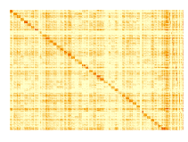
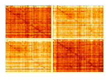
(a) WIOD (left). Zoom of the WIOD submatrix composed of rows and columns of Italy and Spain (right).

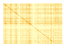
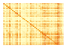
(b) OECD (left). FIGARO (right).

Figure 1: Colored visualization of the elements of the complete I/O tables (year: 2013). For a better visualization, a logarithmic scale is used in the figures.

3.3 Clustering step and simulations

In the case of I/O tables, we argue in the following that a suitable pre-processing step is needed for an effective application of MC. Indeed, as discussed in Subsection 3.2, the main diagonal blocks in the I/O tables ( also called domestic blocks, since each of them refers to trade inside the same country), and especially their entries which refer to exchanges within the same sector and the same country, are characterized by much larger values than the other blocks, which may cause troubles in the application of MC, as the quite different orders of magnitude could make it difficult for MC to have a good generalization capability on both kinds of blocks. Computational reasons (i.e., the need of performing a singular value decomposition step at each iteration of the Soft Impute algorithm) suggest to apply MC to a submatrix associated with a small subset of countries, as this reduces the size of that submatrix. Moreover, as discussed in Subsection 2.2, we argue that MC is more effective when it is applied to an I/O subtable made of “similar” blocks (with respect to the case of “dissimilar” blocks). For this reason, we have decided to apply MC to submatrices of WIOD tables obtained by excluding systematically the main diagonal blocks, where the selection of the countries associated with the submatrices is made by means of hierarchical cluster analysis. In this context, the choice of the number of clusters is determinant and so, in order to validate hierarchical clustering, we perform some simulation exercises, based on synthetic data. We choose to generate our synthetic I/O matrices by adding a matrix of normally distributed random terms $\epsilon$ to the subset of interest of the WIOD dataset, where each element of the matrix $\epsilon_{i,j}\sim\mathcal{N}(0,sd_{\epsilon}),\forall i,\forall j$, $sd_{\epsilon}$ being a Gamma($\alpha$, $\beta$) such that different generated synthetic matrices display different levels of variability. Specifically, we choose $\alpha=1$ and $\beta=1$.

In order to evaluate the correct number of groups in terms of similarity either with respect to input from Italy or with respect to output to Italy, we simulate, respectively: i) $N$ = 1000 synthetic I/O matrices of dimension $56\times 2562$, where 56 is the number of industries in Italy, and 2562 is the product of the 61 industries (final sectors included) and the number of countries except Italy, ii) $N$ = 1000 synthetic I/O matrices of dimension $2562\times 56$, where 2562 is the product of the 61 industries and the number of countries except Italy and 56 is the number of industries in Italy. In order to select the number of clusters we consider the ratio $\frac{WSS}{TSS}$, where $WSS$ is the “Within-cluster sum of squares” and $TSS$ is the “Total sum of squares”. More in details, the optimal number of clusters is the minimum such number for which $\frac{WSS}{TSS}<K$, where $K$ is a cut-off that we set to $0.5$.

It is worth observing that the volume of inputs (outputs) taken from (given to) a specific country is not equally distributed all along other considered countries. Table 2 and Figure 2 show, for the case of inputs from Italy in 2010, a strong dispersion both in terms of averages by countries and in terms of within countries standard deviations. These evidences further motivated us to use AACD as a dissimilarity measure for hierarchical clustering. Table 3 reports the results of the simulation using (stacked) years from 2010 to 2013.

Statistic	Min.	1st Qu.	Median	Mean	3rd Qu.	Max.
Averages by country	0.034	0.488	0.837	1.567	1.780	10.080
Within country st. dev.	0.354	4.034	6.917	10.254	13.097	47.461

Table 2: Distribution of the average exchanges from Italy (in input), by country of output (averages by country) and of the within country standard deviation (within country st. dev.). All countries excluding Italy. WIOD data, year: 2010.

Figure 2: Kernel density curves of the distribution of the average exchanges from Italy (in input), by country of output (averages by country) and of the within country standard deviation (within country standard deviation). All countries excluding Italy. WIOD data, year: 2010.

Direction	Min.	1st Qu.	Median	Mean	3rd Qu.	Max.
Input	14	21	21	21.070	21	28
Output	16	22	22	21.971	22	28

Table 3: Simulation results for the choice of the optimal number of clusters. $N$=1000 replications of hierarchical clustering with complete linkage criterion and AACD as dissimilarity measure, on I/O synthetic matrices derived from WIOD original data. Adopted criterion: $\frac{WSS}{TSS}$. More precisely, we chose the minimum number of clusters such that $\frac{WSS}{TSS}<0.5$. Considering Italy in input and all other countries in output (input), and considering Italy in output and all other countries in input (output). Years: from 2010 to 2013 (4 years).

According to the results in Table 3 we obtain a fairly good clustering with around 21/22 groups. Following these results, in Subsection 3.5 we are going to consider as similar those groups of countries belonging to the same cluster in a configuration with 21 groups (when Italy is in input) or 22 groups (when Italy is in output).

Finally, MC has been applied to I/O subtables associated with suitable groups of “fictitious” similar and dissimilar countries obtained from synthetic matrices, and the performance has turned out to be similar to the one obtained in the case of real data, which is discussed extensively in Subsection 3.5. To ease the reading of the work, results for the case of synthetic matrices are reported later in Appendix A.4.

3.4 Application to forecasting

In this subsection, we consider the application of MC to forecasting. Our focus is not on the absolute RMSE, but on its percentage of reduction (in correspondence of the optimal value of the regularization parameter $\lambda$), with respect to a base case (represented by $\lambda\simeq 0$). The following situation is considered. Starting from WIOD tables relative to some consecutive years, the information associated with a subset of countries is reported in a matrix, keeping only the off-main diagonal blocks, as done at the end of the previous subsection. Then, for one of these ordered pairs of countries, the information about the last year is obscured, and one tries to reconstruct it by MC. As an example, Table 4 refers to the case in which the countries considered are France and Italy, and the years analyzed are 2010, 2011, 2012, 2013, and 2014. All the entries related to France imports in 2014 coming from Italy (i.e., input sectors are from Italy and intermediate/final outputs are from France) are obscured, then such entries are reconstructed by MC. The rationale behind this application is that WIOD tables are obtained by combining information coming from different sources, and these are not necessarily synchronized. So, one could combine the complete information available in the past with the partial one currently available, to predict currently missing elements.

I/O, year
FRA/ITA, 2010	ITA/FRA, 2010
FRA/ITA, 2011	ITA/FRA, 2011
FRA/ITA, 2012	ITA/FRA, 2012
FRA/ITA, 2013	ITA/FRA, 2013
FRA/ITA, 2014	ITA/FRA, 2014

Table 4: Structure of the WIOD submatrix used for the example reported in Figure 3(a). Each block is made of $56$ rows for the inputs (corresponding to the $56$ intermediate sectors considered by WIOD), $56$ columns for the intermediate outputs (one for each intermediate sector), and other $5$ columns for the final products. All the entries contained in the block highlighted in bold are obscured and reconstructed by MC.

Figure 3(a) illustrates the results of the application of the MC Algorithm 1 to the partially-observed WIOD submatrix reported in Table 4 (details about the construction of the training, validation and test sets are provided at the end of Subsection 2.2). The figure shows that, in this case, MC is able to reduce significantly the RMSE of reconstruction on the missing elements in 2015, when moving from the case $\lambda\simeq 0$ (for which the predictions of the missing elements are nearly equal to $0$) to the optimal choice of $\lambda$. More precisely, for $\lambda\simeq 0$, one gets

$$RMSE_{\lambda}^{\rm val} = \sqrt{\frac{1}{|\Omega^{\rm val}|}\sum_{(i,j)\in\Omega^{\rm val}}\left(M_{i,j}-{\color[rgb]{0,0,0}\hat{M}}_{\lambda,i,j}\right)^{2}}$$ (25)

$$\simeq \sqrt{\frac{1}{|\Omega^{\rm val}|}\sum_{(i,j)\in\Omega^{\rm val}}M_{i,j}^{2}}\simeq 86.5711$$

(since, in this case, one gets ${\bf S}_{\lambda}({\bf Y})\simeq{\bf Y}$ from Equation (18), hence every time Step 2.a of Algorithm 1 is performed, one gets a matrix ${\bf\color[rgb]{0,0,0}\hat{M}}^{\rm new}$ whose entries are nearly equal to $0$ in the positions corresponding to unobserved entries of ${\bf M}$). Instead, for the optimal value $\lambda^{\circ}=2^{6}=64$ of $\lambda$ (whose location is highlighted in the figure), one gets

$$RMSE_{\lambda^{\circ}}^{\rm val}\simeq{\color[rgb]{0,0,0}47.2791}\,,$$

obtaining a reduction of the RMSE of about $45\%$. A similar behavior is observed for the RMSE of matrix reconstruction on the test set, the reduction of such RMSE in this case being from $116.0874$ (for $\lambda\simeq 0$) to $51.7544$ (for $\lambda=\lambda^{\circ}$), which amounts at about $55\%$. Hence, a good generalization capability is observed, showing no overfitting occurred in the application of MC. Results in terms of SMAPE are reported in Figure 3(b). The irregular behavior of the curves associated with the SMAPE is due to the fact that MC does not address directly the SMAPE criterion, whereas the RMSE on the training set is part of the objective function of the MC optimization problem (15). Moreover, Figure 3(c) compares the singular values distribution of the WIOD submatrix reported in Table 4, and the one of the completed submatrix produced as output by the algorithm, for both $\lambda\simeq 0$ and the optimal value of $\lambda$. It is evident from the figure that MC was able to reconstruct excellently the singular values distribution of the original WIOD submatrix (part of which was not observed), due to the large overlap of the curves reported in the figure. Moreover, such distribution converges rapidly to $0$, which, as already reported in the Introduction, is a necessary (but not sufficient) condition for a good performance of MC. Indeed, Eckart-Young theorem (see Appendix A.1) provides an upper bound on the performance of MC, for a given number of singular values kept. Finally, Figure 3(d) shows a colored visualization of the elements of the original WIOD submatrix, the positions of the missing entries (highlighted in red), the reconstructed submatrix obtained for the optimal value of the regularization constant $\lambda$, and the element-wise absolute value of the reconstruction error. It is worth recalling that the positions of the missing entries form the union of the validation and test sets, whereas the position of the observed entries form the training set. In this case, although the third column in Figure 3(d) shows that MC looks able to reconstruct some pattern in the missing block of the matrix (with respect to the case $\lambda\simeq 0$, for which the missing block is forecast by a block of all negligible elements), the reconstruction error looks to be still large (fourth column), having a similar pattern as the corresponding original non-obscured block (first column). This is partly due to the fact that a $50\%$ reconstruction error corresponds to a reduction by $1$ in logarithmic scale with base $2$. Improved results are reported in the next subsection (see the next Figures 6(a) and 8(a)), where the choice of the WIOD subtable to which MC is applied is guided by hierarchical clustering.

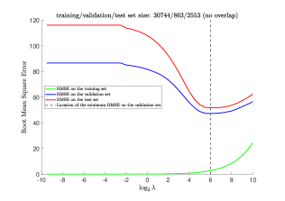
(a) Results (expressed in terms of RMSE) of the application of Algorithm 1 to the WIOD submatrix reported in Table 4.

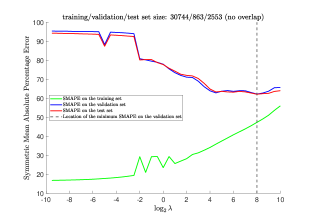
(b) Results (expressed in terms of SMAPE) of the application of Algorithm 1 to the WIOD submatrix reported in Table 4.

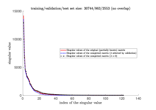
(c) Singular values distribution of the WIOD submatrix reported in Table 4, and the one of the completed submatrix produced by Algorithm 1 for the optimal regularization constant (RMSE criterion).

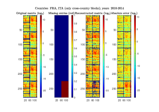
(d) Colored visualization of the elements of the WIOD submatrix reported in Table 4, positions of the missing entries, reconstructed submatrix obtained for the optimal regularization constant (RMSE criterion), and element-wise absolute value of the reconstruction error.

Figure 3:

3.5 Matrix completion applied to groups of similar/dissimilar countries determined by hierarchical clustering

In this subsection, using data from the WIOD latest release, we compare the application of MC to WIOD submatrices obtained using a pre-processing step based on hierarchical clustering. The dissimilarity between any two countries $c_{1}$ and $c_{2}$ is computed as the AACD between the corresponding blocks of $\mathbb{T}$ in the WIOD table (stacked by considering several consecutive years), obtained by either choosing Italian sectors in input and intermediate/final outputs from the two countries $c_{1}$ and $c_{2}$ ( $\mathbb{T}^{Italy,c_{1}}$ and $\mathbb{T}^{Italy,c_{2}}$, recalling the notation introduced in Subsection 2.1), or choosing Italian intermediate/final outputs and sectors from the two countries $c_{1}$ and $c_{2}$ in input ( $\mathbb{T}^{c_{1},Italy}$ and $\mathbb{T}^{c_{2},Italy}$). In other words, the dissimilarity of the two countries $c_{1}$ and $c_{2}$ in their Italian export patterns is evaluated in the first case, whereas their dissimilarity in the respective Italian import patterns is evaluated in the second case. Both the hierarchical clustering analyses are repeated taking as inputs stacked I/O blocks associated with several years (2010, 2011, 2012, and 2013), and using complete linkage to perform clustering. Figures 4 and 5 report the dendrograms obtained, where $c_{1}$ and $c_{2}$ are, respectively, both output countries (Figure 4), and both input countries (Figure 5).

In this way, it is possible to extract from Figure 4 two groups of 4 output countries (see Tables 5 and 6) that are, respectively, in the same cluster, and in 4 different clusters.

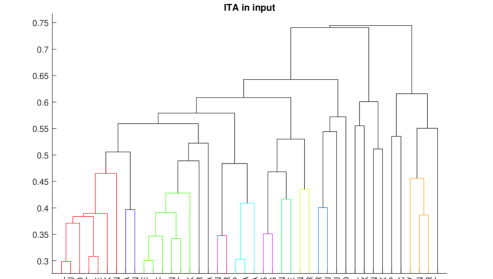
Figure 4: Dendrograms of output countries with Italian sectors in input, based on WIOD tables (stacked over the years 2010–2013). Hierarchical clustering performed with the AACD dissimilarity measure ($y$-axis) and complete linkage. 21 desired groups (compare with Table 3). Countries in the same cluster are depicted with the same color. Countries in singleton clusters are highlighted in black.

Figure 5: Dendrograms of input countries with Italian sectors in output, based on WIOD tables (stacked over the years 2010–2013). Hierarchical clustering performed with the AACD dissimilarity measure ($y$-axis) and complete linkage. 22 desired groups (compare with Table 3). Countries in the same cluster are depicted with the same color. Countries in singleton clusters are highlighted in black.

Table 5 refers to a WIOD submatrix whose blocks have Italian sectors in input and intermediate/final outputs associated the first group of extracted countries (specifically, Austria, Belgium, Germany, and the Netherlands). In contrast, in Table 6, the intermediate/final outputs refer to the second group of extracted countries (specifically, Australia, Belgium, Japan, and Malta). For predictive/matrix completion purposes, the tables contain also data related to the year 2014. Then, the MC Algorithm 1 is applied to both submatrices, after obscuring all the elements of their last block (highlighted in bold in Tables 5 and 6), which refers to a specific output country in 2014.

I/O, year
ITA/AUT, 2010	ITA/BEL, 2010	ITA/DEU, 2010	ITA/NDL, 2010
ITA/AUT, 2011	ITA/BEL, 2011	ITA/DEU, 2011	ITA/NDL, 2011
ITA/AUT, 2012	ITA/BEL, 2012	ITA/DEU, 2012	ITA/NDL, 2012
ITA/AUT, 2013	ITA/BEL, 2013	ITA/DEU, 2013	ITA/NDL, 2013
ITA/AUT, 2014	ITA/BEL, 2014	ITA/DEU, 2014	ITA/NDL, 2014

Table 5: Structure of the WIOD submatrix used for the example reported in Figure 6(a). Similar comments as in Table 4 apply.

I/O, year
ITA/AUS, 2010	ITA/BEL, 2010	ITA/JPN, 2010	ITA/MLT, 2010
ITA/AUS, 2011	ITA/BEL, 2011	ITA/JPN, 2011	ITA/MLT, 2011
ITA/AUS, 2012	ITA/BEL, 2012	ITA/JPN, 2012	ITA/MLT, 2012
ITA/AUS, 2013	ITA/BEL, 2013	ITA/JPN, 2013	ITA/MLT, 2013
ITA/AUS, 2014	ITA/BEL, 2014	ITA/JPN, 2014	ITA/MLT, 2014

Table 6: Structure of the WIOD submatrix used for the example reported in Figure 7(a). Similar comments as in Table 4 apply.

Figures 6(a) and 7(a) report the results of the application of the MC Algorithm 1 to the two WIOD submatrices whose structures are described, respectively, in Tables 5 and 6. As expected, the results show a better performance of the MC algorithm, measured in terms of the percentage of reduction of the RMSE on the validation set from $\lambda\simeq 0$ to the optimal choice of $\lambda$, in the case of the first submatrix, whose intermediate/final outputs are associated with more similar countries.

It is worth observing that quite similar results have been obtained if a different 2014 block corresponding to another country in the group of 4 countries is obscured in each of the two WIOD submatrices, or when the analysis has been repeated by considering Italy in output and 4 similar/dissimilar countries in input (see the dendrogram reported in Figure 5). In this last analysis, the selected subset of 4 similar countries in input is made by Belgium, Germany, Spain, and France (see Table 7), whereas the selected subset of 4 dissimilar countries in input is made by Germany, India, Malta, and Slovenia (see Table 8). Corresponding results of the MC analysis are reported in Figures 8(a) and 9(a). Again, similar comments as before apply: when more similar input countries are considered and the RMSE criterion is considered, the performance of MC improves.

Finally, a comparison of Figures 6(b), 7(b), 8(b), and 9(b) shows that, also when the SMAPE performance measure is used, MC applied to similar countries produces better results (in terms of relative improvement with the respect to the baseline case) than MC applied to dissimilar countries.

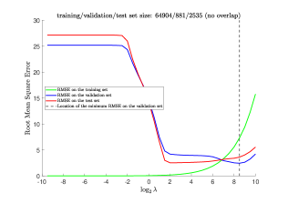
(a) Results (expressed in terms of RMSE) of the application of Algorithm 1 to the WIOD submatrix reported in Table 5.

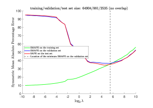
(b) Results (expressed in terms of SMAPE) of the application of Algorithm 1 to the WIOD submatrix reported in Table 5.

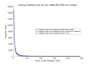
(c) Singular values distribution of the WIOD submatrix reported in Table 5, and the one of the completed submatrix produced by Algorithm 1 for the optimal regularization constant (RMSE criterion).

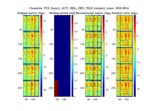
(d) Colored visualization of the elements of the WIOD submatrix reported in Table 5, positions of the missing entries, reconstructed submatrix obtained for the optimal regularization constant (RMSE criterion), and element-wise absolute value of the reconstruction error.

Figure 6:

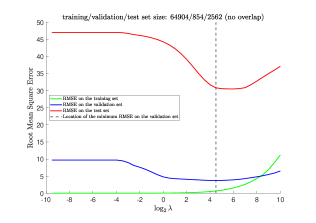
(a) Results (expressed in terms of RMSE) of the application of Algorithm 1 to the WIOD submatrix reported in Table 6.

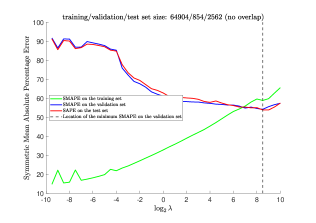
(b) Results (expressed in terms of SMAPE) of the application of Algorithm 1 to the WIOD submatrix reported in Table 6.

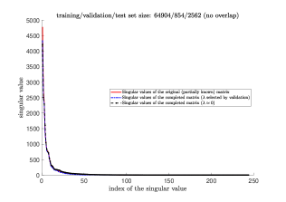
(c) Singular values distribution of the WIOD submatrix reported in Table 6, and the one of the completed submatrix produced by Algorithm 1 for the optimal regularization constant (RMSE criterion).

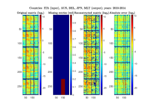
(d) Colored visualization of the elements of the WIOD submatrix reported in Table 5, positions of the missing entries, reconstructed submatrix obtained for the optimal regularization constant (RMSE criterion), and element-wise absolute value of the reconstruction error.

Figure 7:

I/O, year
BEL/ITA, 2010	DEU/ITA, 2010	ESP/ITA, 2010	FRA/ITA, 2010
BEL/ITA, 2011	DEU/ITA, 2011	ESP/ITA, 2011	FRA/ITA, 2011
BEL/ITA, 2012	DEU/ITA, 2012	ESP/ITA, 2012	FRA/ITA, 2012
BEL/ITA, 2013	DEU/ITA, 2013	ESP/ITA, 2013	FRA/ITA, 2013
BEL/ITA, 2014	DEU/ITA, 2014	ESP/ITA, 2014	FRA/ITA, 2014

Table 7: Structure of the WIOD submatrix used for the example reported in Figure 8(a). Similar comments as in Table 4 apply.

I/O, year
DEU/ITA, 2010	IND/ITA, 2010	MLT/ITA, 2010	SVN/ITA, 2010
DEU/ITA, 2011	IND/ITA, 2011	MLT/ITA, 2011	SVN/ITA, 2011
DEU/ITA, 2012	IND/ITA, 2012	MLT/ITA, 2012	SVN/ITA, 2012
DEU/ITA, 2013	IND/ITA, 2013	MLT/ITA, 2013	SVN/ITA, 2013
DEU/ITA, 2014	IND/ITA, 2014	MLT/ITA, 2014	SVN/ITA, 2014

Table 8: Structure of the WIOD submatrix used for the example reported in Figure 9(a). Similar comments as in Table 4 apply.

4 Future research and concluding remarks

This work represents the first attempt to adopt a Matrix Completion (MC) algorithm, combined with hierarchical clustering pre-preprocessing step, to forecast missing entries in submatrices of I/O tables in the context of a panel data analysis.

The particular structure of I/O tables, reported in the article, makes the data reconstruction and forecasting problems not trivial. Hence, in the pre-processing phase, we have employed the dissimilarity pattern of countries to define low-rank I/O subtables with few dominant singular values. A panel matrix completion with nuclear norm penalty has been tested on those low-rank subtables. The effectiveness of the proposed method according to historical data available from previous years has been demonstrated when the considered I/O subtables are obtained by selecting similar countries.

A first possible extension of the analysis concerns comparing matrix reconstruction of I/O tables (in one year, based on current and previous years) based on the repeated application of matrix completion to several subtables of the original I/O table, instead of a single more computationally expensive and (presumably) less effective application to the whole table (possibly after removing domestic blocks, likewise in this article). The proposed methodology is expected to be applicable, with similar results, also to other I/O tables (either industry-by-industry and product-by-product ones), because their structure is often similar to the one of WIOD tables, as highlighted in this work.

As a second possible extension, algorithms for clustering and matrix completion different from those employed in the present article could be used. Moreover, matrix completion itself could be compared with other imputation methods for missing entries in panel data models. A comparison with alternative methods such as the one suggested in Rueda-Cantucheetal2018 is left for future research.

As another possible extension, the approach adopted in the paper could be applied to generate counterfactuals of I/O submatrices: e.g., by predicting how the entries of a suitably-specified input-output submatrix related to Japan would have changed, in case the March 2011 earthquake and tsunami and the successive Fukushima Daiichi nuclear disaster Yonemoto2016 would have not occurred. To do this, one would preliminary need to identify sectors of the economy that were not affected by such events, then obscure (and reconstruct) the entries of that submatrix related to other sectors that, on the contrary, were affected.

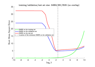
(a) Results (expressed in terms of RMSE) of the application of Algorithm 1 to the WIOD submatrix reported in Table 7.

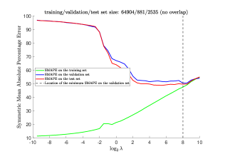
(b) Results (expressed in terms of SMAPE) of the application of Algorithm 1 to the WIOD submatrix reported in Table 7.

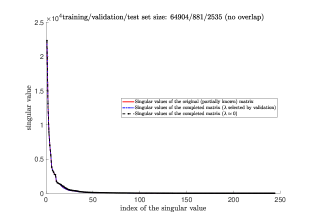
(c) Singular values distribution of the WIOD submatrix reported in Table 7, and the one of the completed submatrix produced by Algorithm 1 for the optimal regularization constant (RMSE criterion).

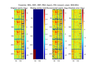
(d) Colored visualization of the elements of the WIOD submatrix reported in Table 7, positions of the missing entries, reconstructed submatrix obtained for the optimal regularization constant (RMSE criterion), and element-wise absolute value of the reconstruction error.

Figure 8:

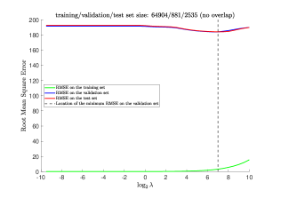
(a) Results (expressed in terms of RMSE) of the application of Algorithm 1 to the WIOD submatrix reported in Table 8.

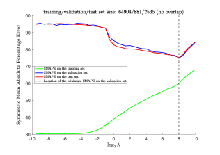
(b) Results (expressed in terms of SMAPE) of the application of Algorithm 1 to the WIOD submatrix reported in Table 8.

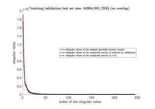
(c) Singular values distribution of the WIOD submatrix reported in Table 8, and the one of the completed submatrix produced by Algorithm 1 for the optimal regularization constant (RMSE criterion).

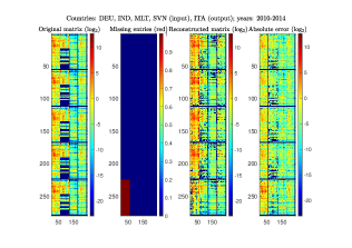
(d) Colored visualization of the elements of the WIOD submatrix reported in Table 8, positions of the missing entries, reconstructed submatrix obtained for the optimal regularization constant (RMSE criterion), and element-wise absolute value of the reconstruction error.

Figure 9:

Declarations

Funding

No external funding

Conflicts of interest/Competing interests (include appropriate disclosures)

No conflicts of interest/competing interest

Availability of data and material (data transparency)

Data are freely available online at www.wiod.org

Code availability (software application or custom code)

Codes are available upon request

Authors’ contributions

(CRediT author statement)

RM: Methodology, Software, Formal Analysis, Investigation, Data Curation, Writing - Original Draft; GG: Validation, Methodology, Software, Formal Analysis, Investigation, Data Curation, Writing - Original Draft; FB: Formal Analysis, Investigation, Writing - Original Draft; MR: Conceptualization, Formal Analysis, Methodology, Resources, Writing - Review & Editing, Supervision, Project Administration. All the authors analysed the results and reviewed the manuscript.

Appendix A Appendix

A.1 Relationship between performance of matrix completion and singular value decomposition of the matrix to be completed

If one indicates by $k$ any non-negative integer smaller than the rank of a rectangular matrix ${\bf M}\in\mathbb{R}^{m\times n}$ (denoted as ${\rm rank}({\bf M})$), then, by Eckart-Young theorem (see, e.g., (Moitra2018, , Theorem 2.1.2)), the best rank-$k$ approximation ${\bf M}_{k}$ of ${\bf M}$ according to the Euclidean norm is provided by the truncated singular value decomposition of ${\bf M}$, in which one keeps only its $k$-largest singular values, and zeroes all the others. Its Root Mean Square Error (RMSE) of reconstruction is equal to

$$RMSE_{k}:=\frac{1}{\sqrt{mn}}\|{\bf M}-{\bf M}_{k}\|_{F}=\frac{1}{\sqrt{mn}}\sum_{i=k+1}^{{\rm rank}({\bf M})}\sigma^{2}_{i}\,,$$ (A1)

being $\sigma_{i}$ (for $i=1,\ldots,{\rm rank}({\bf M})$) the singular values of ${\bf M}$, ordered nonincreasingly. Equation (A1) shows that either a low rank of the matrix to be completed or a fast decay to $0$ of its singular values distribution are important for a successful application of MC to that matrix, as they imply a small right-hand side of the equation. It has to be remarked, however, that they provide only a necessary condition for such a successful application since, in the context of MC, finding exactly the singular value decomposition of the matrix ${\bf M}$ is infeasible, being ${\bf M}$ only partially observed. The reader is referred to Nguyenetlal2019b for more details about properties of a matrix and on the distribution of its sampled elements which allow a successful application of some forms of MC to that matrix. It is worth remarking that some of such properties refer to the possibility of an exact (or “perfect”) reconstruction of the matrix, which is not really needed neither feasible in our specific application of MC to I/O matrices.

A.2 Application of matrix completion to a WIOD submatrix containing both intra-country and inter-country blocks

In Table 9, we consider the following variation of Table 4, in which we take into account also the domestic block associated with Italy, evaluated in different years.

I/O, year
FRA/ITA, 2010	ITA/FRA, 2010	ITA/ITA, 2010
FRA/ITA, 2011	ITA/FRA, 2011	ITA/ITA, 2011
FRA/ITA, 2012	ITA/FRA, 2012	ITA/ITA, 2012
FRA/ITA, 2013	ITA/FRA, 2013	ITA/ITA, 2013
FRA/ITA, 2014	ITA/FRA, 2014	ITA/ITA, 2014

Table 9: Structure of the WIOD submatrix used for the example reported in Figure 10. Similar comments as in Table 4 apply.

For what concerns the application of MC, due to the different orders of magnitude of the elements contained in the domestic blocks compared to the ones belonging to the other blocks, the range of values for the regularization parameter has been increased for this specific example, by setting $\lambda_{k}=2^{k/2-20}$, for $k=1,\ldots,80$. As highlighted by Figure 10, in this case, the performance of MC is quite bad, likely due to the highly different orders of magnitude of the elements in the various blocks.

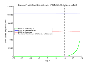
(a) Results (expressed in terms of RMSE) of the application of Algorithm 1 to the WIOD submatrix reported in Table 9.

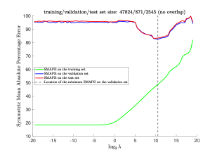
(b) Results (expressed in terms of SMAPE) of the application of Algorithm 1 to the WIOD submatrix reported in Table 9.

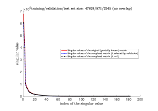
(c) Singular values distribution of the WIOD submatrix reported in Table 9, and the one of the completed submatrix produced by Algorithm 1 for the optimal regularization constant (RMSE criterion).

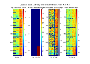
(d) Colored visualization of the elements of the WIOD submatrix reported in Table 9, positions of the missing entries, reconstructed submatrix obtained for the optimal regularization constant (RMSE criterion), and element-wise absolute value of the reconstruction error.

Figure 10:

A.3 Alternative displacement of the blocks

It is worth observing that the several blocks of the WIOD submatrix reported in Table 4 have been displaced in such a way to make the application of MC possible. To clarify this issue, an alternative displacement is reported in Table 10.

I/O, year
FRA/ITA, 2010
ITA/FRA, 2010
FRA/ITA, 2011
ITA/FRA, 2011
FRA/ITA, 2012
ITA/FRA, 2012
FRA/ITA, 2013
ITA/FRA, 2013
FRA/ITA, 2014
ITA/FRA, 2014

Table 10: Alternative displacement of the blocks for the WIOD submatrix reported in Table 4. All the entries contained in the block highlighted in bold are obscured. In this case, the optimization problem (15) is trivial.

In this second case, some rows of the submatrix are obscured as a whole, and the optimal solution to the optimization problem (15) is trivial, in the sense that the obscured rows are reconstructed by setting all their elements to $0$. Indeed, given a partially observed matrix ${\bf P}_{\Omega^{\rm tr}}({\bf M})$ and setting $\varepsilon$ to $0$ and $N^{\rm it}$ by $+\infty$ in Algorithm 1, it is well known from the convergence of that algorithm (see (Mazumder2010, , Lemma 5)) that the sequence of solutions ${\bf\hat{M}}^{\rm new}$ it generates tends to an optimal solution ${\bf\hat{M}}_{\lambda^{\circ}}$ of the optimization problem (15). In case the $i$-th row of ${\bf M}$ is not observed, one can show that all the elements in the same $i$-th row of each matrix ${\bf\hat{M}}^{\rm new}$ generated by the algorithm (which is renamed as ${\bf\hat{M}}^{\rm old}$ at the end of the corresponding iteration) are equal to $0$. Then, by induction and convergence, also all the elements in the $i$-th row of ${\bf\hat{M}}_{\lambda^{\circ}}$ are equal to $0$. More generally, the problem addressed by low-rank MC is either trivial (if a regularization term is present) or ill-posed (if there is no regularization term) when some rows or columns of the matrix to be completed are obscured as a whole, since the other rows/columns provide no information on the obscured ones CandesTao2010 . In both cases, the application of MC becomes meaningless.

In our specific application of MC to I/O subtables, the arrangement of blocks reported in Table 4 makes this issue of triviality/ill-posedness of the problem addressed by MC disappear (while such issue is present in the case of the arrangement of blocks reported in Table 10). This can be justified as follows. In the case of Table 4, the particular arrangement of the blocks makes it possible for MC to “learn”, if present, a relationship between the observed blocks “FRA/ITA, $x$” and “ITA/FRA, $x$” in the same year $x$, where $x=2010,2011,2012,2013$. Then, when the block “FRA/ITA, 2014” is observed, such a relationship makes it possible to estimate (although with some error) the block “ITA/FRA, 2014”, which is not observed. In the case of Table 10, the different arrangement of the same blocks makes impossible for MC to “learn” the relationship above, so the MC estimate of the block “ITA/FRA, 2014” is now arbitrary.

It is worth mentioning that the above-mentioned issue of triviality/ill-posedness of the problem addressed by MC does not actually arise from possibly having either a row or a column made of all zeros in the matrix to be completed, but from the fact of observing no element in such row or column. For simplicity, in the following we illustrate this issue for the case in which one looks for a completed matrix $\hat{\bf M}$ having zero error on the set of observed entries (this is not exactly the case considered in the paper, in which a nonzero error is actually allowed, but the two settings are clearly related, as the first one arises as a limiting case of the optimization problem (15) when $\lambda$ tends to $0^{+}$). So, suppose that one knows that the matrix ${\bf M}$ to be completed has rank $1$, and let the symbol $*$ be used to denote each of its unobserved entries. If ${\bf M}=\begin{bmatrix}1&2\\ *&0\\ 3&*\end{bmatrix}$, then its unique rank-$1$ reconstruction (with no error in the observed entries) is $\hat{\bf M}=\begin{bmatrix}1&2\\ 0&0\\ 3&6\end{bmatrix}$. Instead, if one has ${\bf M}=\begin{bmatrix}1&2\\ 0&0\\ *&*\end{bmatrix}$, then there is no unique rank-$1$ reconstruction of that matrix. On the other hand, taking an arbitrary such reconstruction would be useless.

A.4 Performance of matrix completion on simulated matrices

In this last appendix, we show that the application of MC on the simulated data of Subsection 3.3 produces similar results as its application to the original data. In the following, for illustrative purposes, we focus just on one of the simulated matrices considered in that subsection (in the next figures, the synthetic countries are still named as the original countries, since their respective data are obtained by perturbations of the ones of the associated original countries).

Figures 11 and 12 show the results of the hierarchical clustering, obtained respectively with Italy in input and in output.

Figure 11: Dendrograms of synthetic output countries with Italian sectors in input, based on synthetic WIOD tables (stacked over the years 2010–2013). Hierarchical clustering performed with the AACD dissimilarity measure ($y$-axis) and complete linkage. 21 desired groups (compare with Table 3). Countries in the same cluster are depicted with the same color. Countries in singleton clusters are highlighted in black.

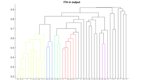
Figure 12: Dendrograms of synthetic input countries with Italian sectors in output, based on synthetic WIOD tables (stacked over the years 2010–2013). Hierarchical clustering performed with the AACD dissimilarity measure ($y$-axis) and complete linkage. 22 desired groups (compare with Table 3). Countries in the same cluster are depicted with the same color. Countries in singleton clusters are highlighted in black.

Then, based on the dendrogram shown in the Figure 11, Figure 13 compares the MC performance (for short, limiting to the RMSE criterion) for the cases – analogous to the ones considered in Subsection 3.5 – in which the 4 selected synthetic countries belong respectively to the same cluster (similar synthetic countries: ESP, FRA, GBR, USA, obscured one in the last year: ESP) and to different clusters (dissimilar synthetic countries: CYP, ESP, IDN, MEX, obscured one in the last year: CYP). Analogously, based on the dendrogram shown in the Figure 12, Figure 14 compares the MC performance (again, limiting to the RMSE criterion) for the cases – analogous to the ones considered in Subsection 3.5 – in which the 4 selected synthetic countries belong respectively to the same cluster (similar synthetic countries: BEL, DEU, ESP, FRA, obscured one in the last year: BEL) and to different clusters (dissimilar synthetic countries: CZE, DEU, EST, IND, obscured one in the last year: DEU). The results are qualitatively similar to the ones reported in for the original data, and demonstrate the robustness of the proposed approach of analysis, which combines hierarchical clustering and MC. Similar results, not reported here due to space constraints, are obtained when the SMAPE criterion is used to compare the performance of MC for similar and dissimilar countries.

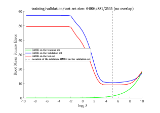
(a) Results (expressed in terms of RMSE) of the application of Algorithm 1 to one synthetic WIOD submatrix made of 4 similar synthetic countries, with Italy in input.

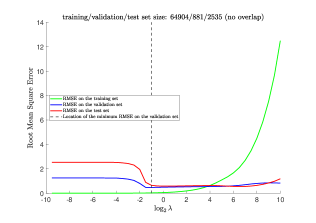
(b) Results (expressed in terms of RMSE) of the application of Algorithm 1 to one synthetic WIOD submatrix made of 4 similar synthetic countries, with Italy in input.

Figure 13:

(a) Results (expressed in terms of RMSE) of the application of Algorithm 1 to one synthetic WIOD submatrix made of 4 similar synthetic countries, with Italy in output.

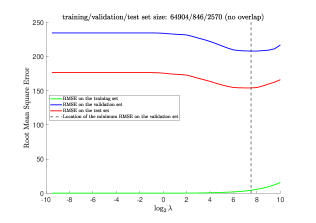
(b) Results (expressed in terms of RMSE) of the application of Algorithm 1 to one synthetic WIOD submatrix made of 4 dissimilar synthetic countries, with Italy in output.

Figure 14:

References

- (1) Aggarwal, C. C., & Reddy, C. K., Eds., Data clustering: Algorithms and applications. Chapman & Hall/CRC Press, London (2014)
- (2) Aldstadt, J., Spatial clustering. In Handbook of applied spatial analysis, pp. 279–300 (Fischer, M. M., & Getis, A., Eds.). Springer, Berlin, Heidelberg (2010)
- (3) Bhattacharya, T., Bhandari, B., & Bairagya, I., Where are the jobs? Estimating skill-based employment linkages across sectors for the Indian economy: An input-output analysis, Structural Change and Economic Dynamics, 53, 292–308 (2020)
- (4) Candès, E.J., & Tao, T., The power of convex relaxation: Near-optimal matrix completion. IEEE Transactions on Information Theory, 56(5), 2053–2080 (2010)
- (5) Carvalho, V., Aggregate fluctuations and the network structure of intersectoral trade. Working Papers - Universitat Pompeu Fabra. Departamento de Economía y Empresa, 1206(1) (2009)
- (6) Cerina, F., Zhu, Z., Chessa, A., & Riccaboni M., World input-output network. PloS One, 10(7), e0134025 (2015)
- (7) Chen, G. Q., Wu, X. D., Guo, J., Meng, J., & Li, C., Global overview for energy use of the world economy: Household-consumption-based accounting based on the world input-output database (WIOD). Energy Economics, 81, 835–847 (2019)
- (8) Fagiolo, G., Reyes, J., & Schiavo, S., On the topological properties of the world trade web: A weighted network analysis. Physica A: Statistical Mechanics and its Applications, 387(15), 3868–3873 (2008)
- (9) Fernandez-Vazquez, E., A generalized cross entropy formulation for matrix balancing with both positive and negative entries (2016, unpublished)
- (10) Hastie, T., Tibshirani, R., & Wainwright, M., Statistical learning with sparsity: the Lasso and generalizations. CRC Press, New York (2015)
- (11) Iori, G., De Masi, G., Precup, O. V., Gabbi, G., & Caldarelli, G., A network analysis of the Italian overnight money market. Journal of Economic Dynamics and Control, 32(1), 259–278 (2008)
- (12) Lance, G.N. & Williams, W.T., A general theory of classificatory sorting strategies. 1. Hierarchical systems. The Computer Journal, 9 (4), 373–380 (1967)
- (13) Lenzen, M., Kanemoto, K., Moran, D., & Geschke, A., Mapping the structure of the world economy. Environmental Science & Technology, 46(15), 8374-8381 (2012)
- (14) Leontief, W. (Ed.), Input-output economics. Oxford University Press. New York (1986)
- (15) Li, C., & Zhou, H., Svt: Singular value thresholding in MATLAB. Journal of Statistical Software, 81(2), DOI: 10.18637/jss.v081.c02 (2017)
- (16) Liang, S., Qi, Z., Qu, S., Zhu, J., Chiu, A. S., Jia, X., & Xu, M., Scaling of global input–output networks. Physica A: Statistical Mechanics and its Applications, 452, 311–319 (2016)
- (17) MacQueen, J., Some methods for classification and analysis of multivariate observations. In Proceedings of the fifth Berkeley Symposium on Mathematical Statistics and Probability, 1 (14), 281–297 (1967)
- (18) Mazumder, R., Hastie, T., & Tibshirani, R., Spectral regularization algorithms for learning large incomplete matrices. Journal of Machine Learning Research, 11, 2287–2322 (2010)
- (19) McNerney, J., Fath, B. D., & Silverberg, G., Network structure of inter-industry flows. Physica A: Statistical Mechanics and its Applications, 392(24), 6427–6441 (2013)
- (20) Metulini, R., Riccaboni, M., Sgrignoli, P., & Zhu, Z., The indirect effects of foreign direct investment on trade: A network perspective. The World Economy, 40(10), 2193–2225 (2017)
- (21) Moitra, A., Algorithmic aspects of machine learning. Cambridge University Press, Cambridge (2018)
- (22) Murtagh, F., & Legendre, P., Ward’s hierarchical agglomerative clustering method: which algorithms implement Ward’s criterion? Journal of Classification, 31, 274–295 (2014)
- (23) Negahban, S., & Wainwright, M. J., Restricted strong convexity and weighted matrix completion: Optimal bounds with noise. Journal of Machine Learning Research, 13(1), 1665–1697 (2012)
- (24) Nguyen, L.T., Kim, J., Kim, S., & Shim, B., Localization of IoT networks via low-rank matrix completion. IEEE Transactions on Communications, 67(8): 5833–5847 (2019)
- (25) Nguyen, L.T., Kim, J., & Shim, B., Low-rank matrix completion: A contemporary survey. IEEE Access, 7: 94215–94237 (2019)
- (26) OECD, Input-Output Tables. For download at http://oe.cd/i-o. Organisation for Economic Co-operation and Development, Paris (2018)
- (27) Oliva, G., Setola, R., & Panzieri, S., Critical clusters in interdependent economic sectors: A data-driven spectral clustering analysis. The European Physical Journal Special Topics, 225: 1929–-1944 (2016)
- (28) Pavia, J. M., Cabrer, B., & Sala, R., Updating input–output matrices: assessing alternatives through simulation. Journal of Statistical Computation and Simulation, 79(12), 1467–1482 (2009)
- (29) Percoco, M., Hewings, G., & Senn, L., Structural change decomposition through a global sensitivity analysis of input-output models. Economic Systems Research, 18(2): 115–131 (2006)
- (30) Rémond-Tiedrez, I., & Rueda-Cantuche, J. M., Full international and global accounts for research in input-output analysis (FIGARO). Eurostat (2019)
- (31) Revelle, W., Hierarchical cluster analysis and the internal structure of tests. Multivariate Behavioral Research, 14(1), 57–74 (1979)
- (32) Riccaboni, M., Wang, X., & Zhu, Z., Firm performance in networks: The interplay between firm centrality and corporate group size. Journal of Business Research, 129(C), 641–653 (2021)
- (33) Rousseeuw, P. J., Silhouettes: a graphical aid to the interpretation and validation of cluster analysis. Journal of Computational and Applied Mathematics, 20, 53–65 (1987)
- (34) Rueda-Cantuche, J. M., Amores, A. F., Beutel, J., & Remond-Tiedrez, I., Assessment of European use tables at basic prices and valuation matrices in the absence of official data. Economic Systems Research, 30(2), 252–270 (2018)
- (35) Sgrignoli, P., Metulini, R., Schiavo, S., & Riccaboni, M., The relation between global migration and trade networks. Physica A: Statistical Mechanics and its Applications, 417, 245–260 (2015)
- (36) Thorndike, R. L., Who belongs in the family?. Psychometrika, 18(4), 267–276 (1953)
- (37) Tibshirani, R., Regression shrinkage and selection via the Lasso. Journal of the Royal Statistical Society. Series B (Methodological), 58(1), 267–288 (1996)
- (38) Tibshirani, R., Walther, G., & Hastie, T., Estimating the number of clusters in a data set via the gap statistic. Journal of the Royal Statistical Society: Series B (Statistical Methodology), 63(2), 411–423 (2001)
- (39) Timmer, M. P., Dietzenbacher, E., Los, B., Stehrer, R., & De Vries, G. J., An illustrated user guide to the world input–output database: the case of global automotive production. Review of International Economics, 23(3), 575–605 (2015)
- (40) Timmer, M. P., Los, B., Stehrer, R., & De Vries, G. J., An anatomy of the global trade slowdown based on the WIOD 2016 release. GGDC research memorandum number 162, University of Groningen, available online at the following hyperlink: https://www.rug.nl/ggdc/html_publications/memorandum/gd162.pdf (2016)
- (41) Tukker, A., De Koning, A., Wood, R., Hawkins, T., Lutter, S., Acosta, J., Rueda Cantuche, M., Bouwmeester, M., Oosterhaven, J., Drosdowski, T., & Kuenen, J., EXIOPOL–development and illustrative analyses of a detailed global MR EE SUT/IOT. Economic Systems Research, 25(1), 50–70 (2013)
- (42) United Nations, Handbook on supply and use tables and input-output tables with extensions and applications (2018)
- (43) Valderas-Jaramillo, J. M., Rueda-Cantuche, J. M., Olmedo, E., & Beutel, J., Projecting supply and use tables: new variants and fair comparisons. Economic Systems Research, 31(3), 423–444 (2019)
- (44) Valderas-Jaramillo, J. M., Rueda-Cantuche, J. M., & Beutel, J., The Euro and SUT-RAS methods: some further considerations. Economic Systems Research, 33(2), 276–286 (2021)
- (45) Wang, H., Wang, C., Zheng, H., Feng, H., Guan, R., & Long, W., Updating input–output tables with benchmark table series. Economic Systems Research, 27(3), 287–305 (2015)
- (46) Wang, H., Ding, L., Guan, R., & Xian, Y., Effects of advancing internet technology on Chinese employment: a spatial study of inter-industry spillovers. Technological Forecasting and Social Change, 161, 120259 (2020)
- (47) Wen, S., Xu, F., & Wen, Z., Robust linear optimization under matrix completion. Science China Mathematics, 57(4), 699–710 (2014)
- (48) Xu, M., & Liang, S., Input–output networks offer new insights of economic structure. Physica A: Statistical Mechanics and its Applications, 527, 121178 (2019)
- (49) Xu, F., Lin, C., He, G., & Wen, Z., Nonnegative matrix completion for life-cycle assessment and input-output analysis. CER working paper, available online at the following hyperlink: http://www.cer.sdu.edu.cn/info/1093/3013.htm (2014)
- (50) Yonemoto, K., Changes in the input–output structures of the six regions of Fukushima, Japan: 3 years after the disaster. Journal of Economic Structures, 5(1), 2 (2016)
- (51) Zhu, Z., Puliga, M., Cerina, F., Chessa, A., & Riccaboni, M., Global value trees. PloS One, 10(5), e0126699 (2015)
- (52) Zhu, Z., Morrison, G., Puliga, M., Chessa, A., & Riccaboni, M., The similarity of global value chains: A network-based measure. Network Science, 6(4), 607–632 (2018)