Comparison of the Parkes and FAST FRB DM Distribution

Abstract

We model the Fast Radio Burst (FRB) dispersion measure (DM) distribution for the Five-hundred-meter Aperture Spherical Telescope (FAST) and compare this with the four FRBs published in the literature to date. We compare the DM distribution of Parkes and FAST, taking advantage of the similarity between their multibeam receivers. Notwithstanding the limited sample size, we observe a paucity of events at low DM for all evolutionary models considered, resulting in a sharp rise in the observed cumulative distribution function (CDF) in the region of $1000\lesssim\mathrm{DM}\lesssim 2000$ pc cm^-3. These traits could be due to statistical fluctuations ($0.12\leq p\leq 0.22$), a complicated energy distribution or break in an energy distribution power law, spatial clustering, observational bias or outliers in the sample (e.g., an excessive $\mathrm{DM}_{\mathrm{Host}}$ as recently found for FRB 20190520B). The energy distribution in this regime is unlikely to be adequately constrained until further events are detected. Modelling suggests that FAST may be well placed to discriminate between redshift evolutionary models and to probe the helium ionisation signal of the IGM.

1 Introduction

The FRB population has been established as being cosmological in nature, with dispersion measures (DMs) typically comprising dominant contributions attributable to propagation through the intergalactic medium (IGM). Under such circumstances, it is viable to use the measured FRB DM as a proxy for redshift (see Macquart et al., 2020, and references therein).

In a previous work (Arcus et al., 2020, hereinafter Paper I), we utilised the  M&E 2018 model of Macquart & Ekers (2018b) to compare the FRB DM distributions, determined from Parkes and ASKAP radio telescope samples, to infer the common FRB population parameters of fluence spectral index, $\alpha$, and the energy function slope, $\gamma$, assuming a power law energy function. Therein we further assumed the telescopes observed the same FRB population and made use of the fact that the telescopes had different survey fluence limits, $F_{0}$ (Arcus et al., 2020). We found: i) no evidence that the FRB population evolves faster than linearly with respect to the cosmic star formation rate (CSFR) for the population sample analysed; ii) the spectral index and energy curve slope were degenerate; and iii) the modelled ASKAP and Parkes DM distributions were consistent with a range of source evolution models.

In this work, we utilise, a priori, these same fitted parameters to model the DM distribution predicted to be observed by FAST – the Five-hundred-meter Aperture Spherical Telescope (see, e.g., Li et al., 2018; Zhu et al., 2020; Niu et al., 2021b). We admit FAST samples in order to introduce higher sensitivity readings, thereby probing deeper into the Universe and enhancing observational discrimination. Moreover, given that Parkes and FAST utilise a nearly identical multibeam receiver (19 versus 13 beams), this permits a similar analysis to be undertaken in order to reduce systematic errors.

We extend the approach described in Paper I  by accounting for the telescope beam pattern, generalising the fitted sensitivity relation of the telescope’s back-end and by accounting for temporal smearing following the approach of Cordes & McLaughlin (2003).

Furthermore, we examine the FRB DM distribution predicted to be detected by FAST, and compare these results with the published FAST FRB event data, noting that, hitherto, only a very limited FRB event sample is available.

In §2, we describe modifications made to the DM distribution model and we compare the resultant distributions with published FRB events. In §3 and §4 we discuss, respectively, the implications of our results (which may have relevance to SKA1-mid) and our conclusions.

2 The DM Distribution

The  M&E 2018 model is principally based on relating the DM distribution, $dR_{F}/d\mathrm{DM}$, to the redshift distribution, $dR_{F}/dz$, for fluences above a survey fluence limit, $F_{0}$, via eq.(1) and eq.(2), and assuming that redshift, $z$, and $\mathrm{DM}$ are bijective for a homogeneous IGM (i.e., one-to-one hence $z\cong\mathrm{DM}$, Macquart & Ekers, 2018b). Here

$$\begin{split}\dfrac{dR_{F}}{dz}&(F_{\nu}>F_{0},z)=4\pi D_{H}^{5}\left(\dfrac{D_{M}}{D_{H}}\right)^{4}\dfrac{(1+z)^{\alpha-1}}{E(z)}\psi_{n}(z)\\ &\dfrac{(1+z)^{2-\alpha}}{4\pi D_{L}^{2}(z)}\begin{cases}0&F_{0}>F_{\mathrm{max}}\\ \left(\dfrac{F_{\mathrm{max}}^{1-\gamma}-F_{0}^{1-\gamma}}{F_{\mathrm{max}}^{1-\gamma}-F_{\mathrm{min}}^{1-\gamma}}\right)&F_{\mathrm{min}}\leq F_{0}\leq F_{\mathrm{max}}\\ 1&F_{0}<F_{\mathrm{min}}\end{cases}\end{split}$$ (1)

and

$$\dfrac{dR_{F}}{d\mathrm{DM}}(F_{\nu}>F_{0},z)=\dfrac{dR_{F}}{dz}(F_{\nu}>F_{0},z)/\dfrac{d\overline{\mathrm{DM}}}{dz}(z)\mathrm{,}$$ (2)

where $R_{F}$ is the (fluence) differential FRB event rate in the observer’s frame of reference per unit solid angle. Other symbol definitions relevant to the model are listed in Table 4.

Here, the CSFR, $\psi_{n}(z)$, has been adopted from Madau & Dickinson (2014) and the mean DM of an homogeneous IGM, $\overline{\mathrm{DM}}(z)$, from (Ioka, 2003); they are respectively given by equations eq.(3) and eq.(4) thus

$$\psi_{n}(z)=K\left(\dfrac{0.015(1+z)^{2.7}}{1+((1+z)/2.9)^{5.6}}\right)^{n}\mathrm{yr^{-1}Mpc^{-3}}$$ (3)

and

$$\begin{split}\overline{\mathrm{DM}}(z)=&\dfrac{3H_{0}c\Omega_{b}}{8\pi Gm_{p}}\\ &\int_{0}^{z}\dfrac{(1+z^{\prime})\left[\frac{3}{4}X_{\mathrm{e,H}}(z^{\prime})+\frac{1}{8}X_{\mathrm{e,He}}(z^{\prime})\right]}{\sqrt{(1+z^{\prime})^{3}\Omega_{m}+\Omega_{\Lambda}}}dz^{\prime}\text{.}\end{split}$$ (4)

The index, $n$, of eq.(3) relates to three redshift evolutionary scenarios: $n=0$ – none; $n=1$ – linear; and $n=2$ – quadratic evolution with respect to the CSFR.

Consistent with Arcus et al. (2020) and throughout this work, we take the ionised fraction of Hydrogen and Helium to be $X_{\mathrm{e,H}}=1$ for $z<8$ and $X_{\mathrm{e,He}}=1$ for $z<2.5$ respectively, or zero otherwise. We take $\alpha$ to refer to the fluence spectral index, defined such that $F_{\nu}\propto\nu^{-\alpha}$, and we assume a $\Lambda$CDM universe consistent with the Planck Collaboration et al. (2014) – i.e., $(h,\>H_{0},\>\Omega_{b},\>\Omega_{m},\>\Omega_{\Lambda},\>\Omega_{k})=(0.7,\>100\>h\,\mathrm{kms}^{-1}\mathrm{Mpc}^{-1},\>0.049,\>0.318,\>0.682,\>0)$.

2.1 Model Extensions

To better account for instrumental effects, we extend the model by: i) generalising the sensitivity formulation using the method introduced by Cordes & McLaughlin (2003), to allow for ready generalisation to different telescopes; and ii) incorporating the effect of the beam function on fluence limit, hence on the population probed (see, e.g., Macquart & Ekers, 2018b; Connor, 2019; Luo et al., 2020; James et al., 2021).

2.1.1 Instrument Response

Since the limiting fluence of a survey is a function of DM, hence redshift (Arcus et al., 2020), we make the substitution given by eq.(5), by including the telescope beam function, $B(\theta)$. We normalise the mean search sensitivity, $\overline{\eta}(z)$, by interpreting $F_{0}$ as $F_{0}(z=0)$. The sensitivity at $\mathrm{DM}=0$ is not important in this context as we are principally concerned with comparing relative event rates via the DM distribution curve shape. (The mean search sensitivity accounts for the mean loss of sensitivity due to DM smearing of the FRB at redshift, $z$. Furthermore, and throughout this work, we take DM to be synonymous with the $\mathrm{DM}_{\mathrm{IGM}}$ , determined from the DM budget unless specifically noted otherwise.)

$$F_{0}(z)\rightarrow F_{0}(z,\theta)=\left\{F_{0}/(\overline{\eta}(z)B(\theta)):\overline{\eta}(z=0)=1\right\}\text{.}$$ (5)

Integrating eq.(2) over the telescope’s Field of View (FoV) yields

$$\begin{split}\dfrac{dR_{F}}{d\mathrm{DM}}(F_{\nu}>F_{0}(z,\theta))=&\\ \int_{0}^{2\pi}\int_{0}^{\theta_{b}}\dfrac{dR_{F}}{dz}/&\dfrac{d\overline{\mathrm{DM}}}{dz}\cdot\sin\theta d\theta d{\phi}\mathrm{,}\end{split}$$ (6)

where $\theta_{b}$ is the applicable beam integration limit.

For a detected burst of width, $w$, the detection sensitivity varies as $w^{-1/2}$ (Cordes & McLaughlin, 2003), resulting from the burst energy being spread over time. Here, we are primarily interested in DM-dependent effects, introduced by different spectral and temporal resolutions used for incoherent de-dispersion searches. The effects of scattering are included in the distribution of FRB widths modelled in Paper I, so that only differences in FRB widths (e.g. due to scattering) between Parkes and FAST will skew our model. There is, however, no evidence for a correlation between DM and scattering (see, e.g., Amiri et al., 2021, §7.3) and it is unclear in which direction a correlation would trend (see e.g. discussion in James et al., 2021) and we do not expect a significant effect. We therefore ignore such effects and assume a constant width distribution. In order to generalise the formulation of sensitivity to other telescopes, we utilise a general form thus

$$\eta(\mathrm{\mathrm{DM}},w)=\dfrac{\eta_{0}}{\sqrt{\left(\frac{8.3\mathrm{DM}\Delta\nu}{10^{3}\nu_{c}^{3}w}\right)^{2}+\left(\frac{\Delta t}{w}\right)^{2}+1}}\text{,}$$ (7)

where $\nu_{c}$ is the observing centre frequency and $\eta(\mathrm{DM},w)$, $\Delta\nu$ and $\Delta t$ are the instrument’s back-end sensitivity, bandwidth and time resolution respectively.

The FRB pulse-width is assumed to follow a log normal distribution with mean sensitivity given by eq.(8), where the maximum burst search width, $w_{m}$, is taken to be $32\,\mathrm{ms}$ (Arcus et al., 2020).

$$\begin{split}\bar{\eta}({\mathrm{DM}})=\dfrac{1}{\sqrt{2\pi}\ln\sigma}\int_{0}^{w_{m}}&w^{-\frac{3}{2}}\eta(\mathrm{DM},w)\\ &e^{-(\ln w-\ln\mu)^{2}/(2\ln^{2}\sigma)}dw\mathrm{,}\end{split}$$ (8)

and the burst-width mean and standard deviation are given, respectively, by $\mu$ and $\sigma$.

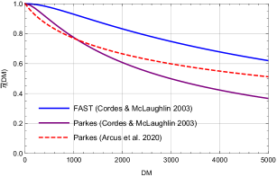
Figure 1: The normalised mean efficiency for Parkes and FAST using eq.(8) (Cordes & McLaughlin, 2003) and the telescope parameters of Table 2. For reference, we include the normalised mean efficiency curve attained for Parkes, using the best-fit method detailed in Arcus et al. (2020).

2.1.2 Beam Pattern

In order to incorporate the beam pattern into the model, we first assess the analytic forms for the Airy relative to the Gaussian beam functions for Parkes, given the similarities in the antenna feeds between the two telescopes. The Airy and Gaussian beam functions utilised are given by eq.(9) and eq.(10) respectively

$$B(\theta)=\left(\dfrac{2{\mathrm{J}}_{1}(ka\sin\theta)}{ka\sin\theta}\right)^{2}$$ (9)

and

$$B(\theta)=A\exp\left[-\frac{\theta^{2}}{2\theta_{b}^{\prime 2}}\right]+(1-A)\left[-\frac{\theta^{2}}{2\theta_{r}^{\prime 2}}\right]$$ (10)

where $\mathrm{J}_{1}(x)$ is the Bessel function of the first kind of order 1, $k$ the wave number at the receiver centre frequency, $\nu_{c}$, $a$ the Airy disc radius and $\theta$ the off bore-sight angle to the source.

We utilise the Gaussian formulation of Macquart & Ekers (2018a, see Figure 5 and eq.(8) therein), where $1-A=0.0015$, $\theta^{\prime}_{b}=(14^{\prime}/3)/\sqrt{2\ln{2}}$ and $\theta^{\prime}_{r}=(1.5^{\circ}/2)/\sqrt{2\ln{2}}$. The additional term of the Gaussian beam function is introduced for Parkes in order to account for the off-axis response that extends scattering out to approximately $1.5^{\circ}$. This effect is due to the pedestal and its side-lobes, resulting from scattering from the base of the $6\mathrm{m}$ focus cabin, which is not included in the Airy beam (Macquart & Ekers, 2018a).

Given FAST will not incur the same pedestal and cabin scattering effects, since the dish is much larger than similarly sized antenna feed blockage at the focus, and that the DM distribution is generally insensitive to the form of the beam function (James et al., 2021), we choose to use the Airy function in our modelling.

2.1.3 Burst Energy Distribution

We use a reference source of 10 Jy ms at $z=1$ with fluence spectral index $\alpha=0$ throughout our modelling. Furthermore, we assume an energy function described by a power law given by eq.(11) (Macquart & Ekers, 2018b; Arcus et al., 2020)

$$\theta_{E}(E_{\nu};\gamma)=\dfrac{\gamma-1}{E^{1-\gamma}_{\mathrm{min}}-E^{1-\gamma}_{\mathrm{max}}}E^{-\gamma}_{\nu}\mathrm{,}$$ (11)

where $\theta_{E}$ is the event rate energy function.

We choose an energy function spanning seven decades, i.e., $\sim 1.28\times\left[10^{22},10^{29}\right]$  J Hz^-1 , encompassing the upper region found by Shannon et al. (2018, see their Figure 2 wherein an absence of sources above $\sim 10^{27}$ J Hz^-1 is noted).

The minimum, $F_{\mathrm{min}}$, and maximum, $F_{\mathrm{max}}$, fluences corresponding to $E_{\mathrm{min}}$ and $E_{\mathrm{max}}$ respectively, are related via eq.(12)

$$E_{\nu}(F_{\nu},z;\alpha)=\dfrac{4\pi D_{L}^{2}(z)}{(1+z)^{2-\alpha}}F_{\nu}\mathrm{,}$$ (12)

where $D_{L}(z)$ is the luminosity distance at redshift, $z$.

Li et al. (2021) have reported a bimodal energy distribution inferred from multiple pulses of the repeater FRB 121102 using FAST. The extent to which the energy distribution of this particular object reflects the energy distribution of the entire population is unclear. We note that at high energies the energy distribution of FRB 121102 is similar to that of a power-law, hence we retain the power-law in our modelling.

We initially conduct a DM distribution re-fit for Parkes and ASKAP events using the original FRB event data and model of Paper I, treating  $E_{\mathrm{max}}$ as a free parameter. The fitted value for  $E_{\mathrm{max}}$ was found to differ only marginally to that assumed in the original work and consistent with both Luo et al. (2020) and James et al. (2018). We therefore retain the same values of  $E_{\mathrm{min}}$ and  $E_{\mathrm{max}}$ per Paper I  (see Table 1). Furthermore, we conduct a preliminary investigation into the effect of utilising a power law versus a Schechter function (see, e.g., Lu & Piro, 2019; Luo et al., 2020) for the energy function. We examine the effect that the different functional forms have on the DM distributions over the chosen energy range and we find no discernible difference between the resultant DM distributions: a result consistent with James et al. (2021). We therefore choose to retain the power law formulation described by eq.(11) in our modelling.

2.2 DM Distribution Modelling

To model the FAST DM distribution, we utilise the FRB population parameter-set determined from Paper I  and listed in Table 1, as determined from simultaneous fits to Parkes and ASKAP data. We do so on the basis of the similarities between the FAST and Parkes telescope back-ends and until an increased sample size, hence improved statistics, become available.

We utilise a pulse-width mean of $\mu=3.44\;\mathrm{ms}$ and standard deviation of $\sigma=3.44\;\mathrm{ms}$ (Arcus et al., 2020). Using these parameters, in conjunction with the telescope parameters of Table 2, we model the DM distribution via eq.(6)

The normalised mean efficiency for Parkes and FAST, via eq.(8), is depicted in Figure 1 along with the normalised mean efficiency for Parkes, using the best-fit method of Paper I. We note that the true response of an FRB detection algorithm is complex and may only be fully determined via FRB injection tests, such as those performed by UTMOST (Gupta et al., 2021). Deficiencies in this formulation are unlikely to have significant consequences for our results since the differences in the low DM range differ by $\lesssim 10\%$ up to $\textrm{DM}\sim 2000$  pc cm^-3 – see Figure 1. This may become increasingly significant at large DM, however, where the analytic formulation may need to be adjusted.

Integration over the FoV is performed by setting the beam integration limit $\theta_{b}=2\cdot\theta_{\text{FWHM}}$, the point of beam overlap given the receiver feed spacing for both telescopes (Staveley-Smith et al., 1996; Dunning et al., 2017).

Table 1: DM distribution model parameters used herein. The FRB population parameters are taken, a priori, from Arcus et al. (2020). The energy function slope, $\gamma$, represents the 68% confidence interval and we adopt the fixed constraint of $\alpha=1.5$ (Macquart et al., 2019).

[b] $n$ $\alpha$^$\dagger$ $\hat{\gamma}$  $E_{\mathrm{min}}$ ^$\dagger$  $E_{\mathrm{max}}$ ^$\dagger$ Evolution ( J Hz^-1 ) Model 0 1.5^$\ddagger$ 1.5 ${}_{-0.2}^{+0.2}$ $1.28\times 10^{22}$ $1.28\times 10^{29}$ None 1 1.5^$\ddagger$ 1.8 ${}_{-0.1}^{+0.1}$ $1.28\times 10^{22}$ $1.28\times 10^{29}$ Linear 2 1.5^$\ddagger$ 2.2 ${}_{-0.1}^{+0.1}$ $1.28\times 10^{22}$ $1.28\times 10^{29}$ Quadratic

• A set constraint.

Table 2: The telescope parameters used to model the DM Distributions for Parkes and FAST. References are: (1) Staveley-Smith et al. (1996); (2) Dunning et al. (2017); (3) Li et al. (2018); (4) Keane et al. (2018); (5) Connor (2019); (6) Luo et al. (2020); & (7) Gardenier & van Leeuwen (2021).

[b] Description Symbol Units FAST Parkes Parameter Reference Parameter Reference Frequency resolution $\Delta\nu$ MHz 0.122 (3) 0.39 (5) Time resolution $\Delta t$ ms 0.196608 (7) 0.064 (5) Observing centre frequency $\nu_{c}$ GHz 1.250 (7) 1.352 (7) FWHM beam-width $\theta_{b}$ ^∘ 0.047 (2) 0.204 (1) Fluence limit (radiometer) $F_{0}$ Jy ms 0.0146 (6) 0.5 (4)

Table 3: The published FAST FRB events used in our analysis.

Designation	$\mathrm{DM}_{\mathrm{Obs}}$	$\mathrm{DM}_{\mathrm{MW}}$	DM Model	Reference
	(pc cm-3)
FRB 181123	1812.0	149.5	YMW16	Zhu et al. (2020)
FRB 181017	1845.2	34.6	NE2001	Niu et al. (2021b)
FRB 181118	1187.7	71.5	NE2001	Niu et al. (2021b)
FRB 181130	1705.5	38.2	NE2001	Niu et al. (2021b)

raphics/ParkesPDF	raphics/FASTPDF
raphics/ParkesCDF	raphics/FASTCDF

Figure 2: The Parkes (left panels) and FAST (right panels) DM distributions as PDFs (top panels) and CDFs (bottom panels). The curve colours relate to redshift evolutionary scenarios: blue, $n=0$, none; purple, $n=1$, linear; and red, $n=2$, quadratic evolution with respect to the CSFR. The Parkes curves were determined by simultaneously fitting multiple population parameters for Parkes and ASKAP data in Arcus et al. (2020), whereas the FAST distributions are predicted using these same fitted population parameters of Table 1. The CDFs are derived from the FRB observations from Parkes and FAST events in the lower panels (black dashed curves). FAST data are listed in Table 3, whilst Parkes event data are drawn from Arcus et al. (2020, Table 1). A Kolmogorov-Smirnov (K-S) test of the FAST event data, with respect to the computed DM distribution for the three evolutionary models, yields p-values of: $p^{\prime}(n=0)=0.22$; $p^{\prime}(n=1)=0.19$; and $p^{\prime}(n=2)=0.12$.

3 Discussion

The Parkes and FAST DM distributions are depicted in Figure 2, as both Probability Density Functions (PDFs) and Cumulative Distribution Functions (CDFs), along with the corresponding CDFs from observed FRB events. The FAST sample is listed in Table 3 and the Parkes sample (depicted for reference purposes) is drawn from Arcus et al. (2020, Table 1).

Parkes DM distribution curves of Figure 2 were determined by simultaneously fitting multiple population parameters between Parkes and ASKAP as undertaken in Paper I. The three evolutionary models for Parkes in Figure 2 are therefore good fits as they use fitted variables. The modelled FAST distributions are, however, predicted, using the same fitted population parameters of Table 1 and the FAST telescope parameters of Table 2. The modelled DM distributions (solid curves) show a similar overall shape and suggest that FAST’s higher sensitivity, compared to other FRB-finding instruments, gives it a superior ability to discriminate between redshift evolutionary models at DM $\gtrsim 1400$ pc cm^-3 .

A Kolmogorov-Smirnov (K-S) test of the FAST observational data, with respect to the modelled DM distributions for the three evolutionary models, yields p-values of: $p^{\prime}(n=0)=0.22$; $p^{\prime}(n=1)=0.19$; and $p^{\prime}(n=2)=0.12$. This indicates there is only mild evidence that the observations are inconsistent with all of the evolutionary models, notwithstanding statistical robustness due to the limited sample size.

The observed FAST DM distribution suggests an apparent paucity of FRB events at low DM (i.e., $\mathrm{DM}\lesssim 1000\text{ pc cm}^{-3}$) in relation to the modelled scenarios, along with a potential sharp rise in the CDF between $1000\text{ pc cm}^{-3}\lesssim\mathrm{DM}\lesssim 2000\text{ pc cm}^{-3}$. None of the evolutionary models predict a paucity of events at low DM, however. This could conceivably be due to a number of factors, including:

1. A complicated energy distribution or break in a single power law distribution function (e.g. a turn-over to a flatter power-law at low energies would reduce the number of near-Universe FRBs).

2. Searches may be biased against either low or high DM events (e.g., a deficit of low-DM FRBs may result from a bias against low-DM events due to RFI discrimination, – see, e.g., Amiri et al. (2021) regarding bias against low DM events due to RFI).

3. The area of sky surveyed with a high-sensitivity telescope may be sufficiently small such that the distribution of FRBs on the sky is non-uniform (i.e., the DM distribution is inhomogeneous due to cosmic variance; such an effect will likely remain untestable until sufficient deep surveys over large areas become available).

4. The FRB sample may contain outliers (e.g., FRB 20190520B has recently been determined to have a large $\mathrm{DM}_{\mathrm{Host}}$ excess, $\mathrm{DM}_{\mathrm{Host}}=903^{+72}_{-111}\mathrm{\,pc\,cm^{-3}}$ Niu et al. (2021a)), which may explain the bulk of the paucity observed given the low number statistics involved).

Event rates are more likely to be affected by evolution at higher look-back times – i.e., at higher redshifts or DMs. We do not consider the low DM paucity to be attributable to evolution in the sensitivity regime of FAST. This raises the interesting prospect of whether a break in the energy function exists. Further samples will be required to break the degeneracy between the evolution models and the energy curve slope: local FRBs with fluence and redshift measurements would be required.

Whilst the CHIME collaboration recently published its first FRB catalogue (Amiri et al., 2021), we note that the CHIME telescope has a very different frequency range to FAST and it is unclear whether these results would be scalable for a comparative analysis. Furthermore, CHIME has a significantly different and complicated beam-pattern that would need to be treated in such an analysis. A new factor, however, is that CHIME provides some evidence for cross correlation between FRBs with large scale cosmic structure (Rafiei-Ravandi et al., 2021): a correlation between galaxies at lower redshift (i.e., $0.3\lesssim z\lesssim 0.5$). Additionally, a correlation of FRBs at higher $\textrm{DM}\sim 800$  pc cm^-3 are noted, which may indicate that FRBs are arriving with DMs higher than expected, potentially resulting in the observed FAST FRB paucity at low-DM and an excess of FRBs with higher DM.

Macquart & Ekers (2018b) discussed at length the potential to detect the helium ionisation signal of the IGM in the redshift and DM distributions using the  M&E 2018 model. We note that this signal is visible in the modelled FAST DM distribution of Figure 2 (top right panel), at $\textrm{DM}\sim 2660$ pc cm^-3 (assumed to occur at $z=2.5$). We therefore expect FAST to be well placed to probe this signature should sufficient FRB events be detected spanning this region of DM-space.

The DM distributions modelled herein do not account for evolution of $\mathrm{DM}_{\mathrm{Host}}$ with redshift. The contributions to the DM of the IGM and host galaxy are inseparable and the problem is unconstrained. The host contribution is often treated as a non-redshift evolving parcel of plasma via the term $\mathrm{DM}_{\mathrm{Host}}/(1+z)$, where $\mathrm{DM}_{\mathrm{Host}}$ is interpreted as dispersion in the host galaxy’s rest frame (see, e.g., Macquart et al., 2020). A detailed investigation of this aspect is out of scope for this paper, and we defer such work to a future paper, which may be explored via simulation.

4 Conclusion

We extend and apply the  M&E 2018 model along with the fitted multiple population parameters determined in Paper I  to the published FAST FRB events in order to compare the predicted DM distributions of FAST with respect to Parkes. We model three redshift evolutionary scenarios and assume a log power law energy function.

Whilst the published FAST sample size is limited, we observe a paucity of events at low DM relative to all evolutionary models, including a sharp rise in the observed CDF in the region of $1000\lesssim\mathrm{DM}\lesssim 2000$ pc cm^-3. (These two traits are not separate effects.) These observations are consistent with statistical fluctuations ($p^{\prime}(n=0)=0.22$; $p^{\prime}(n=1)=0.19$; and $p^{\prime}(n=2)=0.12$). Whilst these traits could be due to a number of factors including statistical fluctuations ($p\leq 0.22$) due to the small sample size, it may point towards a break in the energy function at the low energy regime or to an energy function turn-over.

The energy distribution is unlikely to be able to be adequately determined until further events are detected in this high-sensitivity regime. To break the degeneracy between the energy distribution and redshift evolution, we would require FRBs with similar energy at different redshifts. Identifying rare high-energy FRBs at lower redshift will require large FoV survey telescopes.

FAST has the greatest sensitivity to FRB source evolution in the region $2000\lesssim\mathrm{DM}\lesssim 3000$  pc cm^-3, as indicated by the relative separation of the CDFs for the different evolutionary models in Figure 2, suggesting this would be the best DM region to constrain evolution.

The cooled Parkes Phased Array Feed, currently under construction, will provide up to 88 beams; increasing the FoV by a factor of $\sim 5$ with similar sensitivity as the original Parkes survey and with well-characterised beams. Future instruments such as MeerKAT and later SKA-mid telescopes are expected to approach the sensitivity of FAST with potentially a much larger FoV, should sufficient coherent beams be formed. These instruments should increase the high-redshift FRB sample size thus improving the statistics.

Data availability

Data underlying this article are available within this article.

Appendix A Model Symbols & FRB Population Parameters

A.1 Model Symbols & Fitted Results

Table 4: Symbol definitions relevant to the  M&E 2018 model taken from Arcus et al. (2020) and provided here for convenience.

Symbol	Definition
$G$	Gravitational constant
$m_{p}$	Proton rest mass
$z$	Redshift
$c$	Speed of light in vacuo
$H_{0}$	Hubble constant at the present epoch
$E(z)$	Dimensionless Hubble parameter $E(z)=\sqrt{\Omega_{m}(1+z)^{3}+\Omega_{k}(1+z)^{2}+\Omega_{\Lambda}}$
$H(z)$	Hubble constant at an arbitrary redshift $z:H(z)=H_{0}E(z)$
$D_{H}$	Hubble distance
$D_{M}$	Comoving distance
$D_{L}$	Luminosity distance
$R_{F}$	Total (fluence) differential FRB event rate in the observer’s frame
$\Omega_{m}$	Matter density (baryonic and dark)
$\Omega_{\Lambda}$	Vacuum density
$\Omega_{k}$	Spatial curvature density
$\Omega_{b}$	Baryonic matter density
$\alpha$	Fluence spectral index defined such that $F_{\nu}\propto\nu^{-\alpha}$
$\gamma$	Energy power-law index
$F_{0}$	Fluence survey limit at $\mathrm{DM}=0$
$F_{\mathrm{0,P}}$	Fluence survey limit of the Parkes telescope at $\mathrm{DM}=0$
$F_{\mathrm{0,A}}$	Fluence survey limit of the ASKAP telescope at $\mathrm{DM}=0$
$F_{\nu}$	Fluence (energy spectral density per unit area)
$F_{\mathrm{min}}$	Minimum fluence for luminosity function
$F_{\mathrm{max}}$	Maximum fluence for luminosity function
$E_{\nu}$	Spectral energy density
$E_{\mathrm{min}}$	Lower spectral energy density bound for the event rate energy function
$E_{\mathrm{max}}$	Upper spectral energy density bound for the event rate energy function
$\displaystyle dR_{F}/dz$	Fluence-based redshift distribution
$\displaystyle dR_{F}/d\mathrm{DM}$	Fluence-based DM distribution
$\overline{\mathrm{DM}}(z)$	Mean DM for the homogeneous IGM
$X_{\mathrm{e,H}}$	Fraction of ionised Hydrogen in the homogeneous IGM
$X_{\mathrm{e,He}}$	Fraction of ionised Helium in the homogeneous IGM
$\psi_{n}(z)$	Event rate per comoving volume as a function of redshift: $\psi_{n}(z)\propto\Psi^{n}(z)$
$\Psi(z)$	The cosmic star formation rate (CSFR) per comoving volume
$n$	Exponent of the redshift evolutionary term per comoving volume

References

- Amiri et al. (2021) Amiri M., et al., 2021, ApJS, 257, 59
- Arcus et al. (2020) Arcus W. R., Macquart J.-P., Sammons M. W., James C. W., Ekers R. D., 2020, MNRAS, 501, 5319
- Connor (2019) Connor L., 2019, MNRAS, 487, 5753
- Cordes & McLaughlin (2003) Cordes J. M., McLaughlin M. A., 2003, ApJ, 596, 1142
- Dunning et al. (2017) Dunning A., et al., 2017, in 2017 XXXIInd General Assembly and Scientific Symposium of the International Union of Radio Science (URSI GASS). pp 1–4, doi:10.23919/URSIGASS.2017.8105012
- Gardenier & van Leeuwen (2021) Gardenier D. W., van Leeuwen J., 2021, A&A, 651, A63
- Gupta et al. (2021) Gupta V., et al., 2021, MNRAS, 501, 2316
- Ioka (2003) Ioka K., 2003, ApJ, 598, L79
- James et al. (2018) James C. W., Ekers R. D., Macquart J.-P., Bannister K. W., Shannon R. M., 2018, MNRAS, 483, 1342
- James et al. (2021) James C. W., Prochaska J. X., Macquart J.-P., North-Hickey F. O., Bannister K. W., Dunning A., 2021, MNRAS, 509, 4775
- Keane et al. (2018) Keane E. F., et al., 2018, MNRAS, 473, 116
- Li et al. (2018) Li D., et al., 2018, IEEE Microwave Magazine, 19, 112
- Li et al. (2021) Li D., et al., 2021, Nature, 598, 267–271
- Lu & Piro (2019) Lu W., Piro A. L., 2019, ApJ, 883, 40
- Luo et al. (2020) Luo R., Men Y., Lee K., Wang W., Lorimer D. R., Zhang B., 2020, MNRAS, 494, 665
- Macquart & Ekers (2018a) Macquart J.-P., Ekers R. D., 2018a, MNRAS, 474, 1900
- Macquart & Ekers (2018b) Macquart J.-P., Ekers R., 2018b, MNRAS, 480, 4211
- Macquart et al. (2019) Macquart J. P., Shannon R. M., Bannister K. W., James C. W., Ekers R. D., Bunton J. D., 2019, ApJ, 872, L19
- Macquart et al. (2020) Macquart J. P., et al., 2020, Nature, 581, 391
- Madau & Dickinson (2014) Madau P., Dickinson M., 2014, ARA&A, 52, 415
- Niu et al. (2021a) Niu C. H., et al., 2021a, arXiv e-prints, p. arXiv:2110.07418
- Niu et al. (2021b) Niu C.-H., et al., 2021b, American Astronomical Society, 909, L8
- Planck Collaboration et al. (2014) Planck Collaboration et al., 2014, A&A, 571, A16
- Rafiei-Ravandi et al. (2021) Rafiei-Ravandi M., et al., 2021, ApJ, 922, 42
- Shannon et al. (2018) Shannon R. M., et al., 2018, Nature, 562, 386
- Staveley-Smith et al. (1996) Staveley-Smith L., et al., 1996, Publ. Astron. Soc. Australia, 13, 243
- Zhu et al. (2020) Zhu W., et al., 2020, American Astronomical Society, 895, L6