Scaling dimension of Cooper pair operator from the black hole interior

Abstract

We have shown that in holographic superconductivity theory for 3+1 dimensional system, the scaling dimension of Cooper pair operator can be obtained as a quantized value if we request that the the scalar function describing the order parameter is finite inside the black hole as well as outside. This should be contrasted to the usual situation where we set the mass squared of the scalar by hand. Our method can be applied to any order parameters.

I Introduction

Calculating the anomalous dimension in the interacting field theory is highly non-trivial task. Even in holographic theory[1, 2], scaling dimension has been the input data which was set to be an integer $\Delta=1,2$ by hand. Certainly this is not desirable, because, for example, the scaling dimension of the Cooper pair operator can not be an arbitrary number, and the detailed behavior of the superconductivity depends on this number very sensitively.

In this paper, we analyze the gap equations of holographic superconductors in 3+1 dimension and show that in the presence of the horizon, the regularity of the condensating solution inside the black hole provides a simple way to calculate the scaling dimension, because the higher order singularity requests extra regularity in the solution, leading to the quantized value of the scaling dimension. And we require that the solution is a polynomial after factoring out the singular pieces. Then the solution automatically satisfies the horizon regularity, which is the condition usually imposed in the literature.

We analyzed analytically all the allowed spectrum in the probe limit of the background gravity near the critical temperature. The lowest possible scaling dimension is $\Delta=2$ and the next one is about 3.6.etc. This is analogous to the energy quantization in Schroedinger equation. The generality of our method comes from the ubiquitous appearance of the Heun’s equation in the holographic setup of symmetry breaking regardless of the spin of the matter fields or dimension of the bulk spacetime[1, 2, 3, 4].

II Set up

We consider the action [5],

$${S=\int d^{d+1}x\sqrt{-|g|}\left(-\frac{1}{4}F_{\mu\nu}^{2}-|D_{\mu}\Psi|^{2}-m^{2}|\Psi|^{2}\right),}$$ (1)

where $|g|=\det g_{ij}$, $D_{\mu}\Psi=\partial_{\mu}-igA_{\mu}$ and $F=dA$, and $A=\Phi dt$. Following the ref.[5], we start with the fixed metric of AdS_d+1 blackhole,

$$ds^{2}=-f(r)dt^{2}+\frac{dr^{2}}{f(r)}+r^{2}d\vec{x}^{2},\;\;f(r)=r^{2}\left(1-\frac{r_{h}^{d}}{r^{d}}\right).$$ (2)

In this letter, we will consider only $d=4$ for technical simplicity. The AdS radius is set to be $1$ and $r_{h}$ is the radius of the horizon. The temperature is given by $T=\frac{d}{4\pi}r_{h}$ as usual. The field equations become

$$\frac{d^{2}\Psi}{dz^{2}}-\frac{d-1+z^{d}}{z(1-z^{d})}\frac{d\Psi}{dz}+\left(\frac{g^{2}\Phi^{2}}{r_{h}^{2}(1-z^{d})^{2}}-\frac{m^{2}}{z^{2}(1-z^{d})}\right)\Psi=0,$$

$$\frac{d^{2}\Phi}{dz^{2}}-\frac{d-3}{z}\frac{d\Phi}{dz}-\frac{2g^{2}\Psi^{2}}{z^{2}(1-z^{d})}\Phi=0.$$ (3)

with the coordinate $z=r_{h}/r$. One should notice that the regions $z>1$ and $0<z<1$ are inside and outside of the black hole respectively. Here, $\Psi(z)$ is the scalar field and the electrostatic scalar potential $A_{t}=\Phi$. Near the boundary $z=0$, we have

$$\Psi(z) = z^{\Delta_{-}}\Psi^{(-)}(z)+z^{\Delta_{+}}\Psi^{(+)}(z),$$

$$\Phi(z) = \mu-({\rho}/{r_{h}^{d-2}})z^{d-2}+\cdots$$ (4)

where $\Delta_{\pm}$ are related by $\Delta_{+}+\Delta_{-}=d$ and $\mu$ and $\rho$ are the chemical potential and the charge density, respectively. Once $\Delta$ is determined, $m^{2}$ follows using $m^{2}=\Delta(\Delta-d)$. We restrict ourself to the near critical temperature where probe solution can be trusted [6].

III Near critical temperature

The critical temperature is determined[7] by the the Sturm Liouville eigenvalue $\lambda$. In this section, we will find the relation between $\lambda$, and the scaling dimension $\Delta$. This section is a brief review of our previous work [8].

At the critical temperature $T_{c}$, $\Psi=0$, so Eq.(3) tells us $\Phi^{{}^{\prime\prime}}=0$ near there. Then, we can set [7]

$$\Phi(z)=\tilde{\lambda}r_{c}(1-x)\hskip 28.45274pt\mbox{where}\;\;\tilde{\lambda}=\frac{\rho}{r_{c}^{3}}$$ (5)

where $x=z^{2}$ and $r_{c}$ is horizon radius at the critical temperature. For $T\rightarrow T_{c}$, the field equation $\Psi$ approaches to [8]

$$-\frac{d^{2}\Psi}{dx^{2}}+\frac{1+x^{2}}{x(1-x^{2})}\frac{d\Psi}{dx}+\frac{m^{2}}{4x^{2}(1-x^{2})}\Psi=\frac{\lambda^{2}}{4x(1+x)^{2}}\Psi$$ (6)

where $\lambda=g\tilde{\lambda}$. The critical temperature is given by [7, 8]

$$T_{c}=\frac{d}{4\pi}r_{c}=\frac{1}{\pi}\left(\frac{g\rho}{\lambda}\right)^{\frac{1}{3}},$$ (7)

for $d=4$. Factoring out the behavior near $x=0$ and $x=-1$, we have

$$\Psi(x)=\frac{\left<\mathcal{O}_{\Delta}\right>}{\sqrt{2}r_{h}^{\Delta}}x^{\frac{\Delta}{2}}(1+x)^{-\lambda/2}y(x).$$ (8)

Here, $y$ is normalized by $y(0)=1$ and we obtain

$$\frac{d^{2}y}{dx^{2}}+\left(\frac{\rho_{0}}{x}+\frac{\rho_{1}}{x-1}+\frac{\rho_{2}}{x+1}\right)\frac{dy}{dx}$$

$$+\left(\frac{w_{0}}{x}+\frac{w_{1}}{x-1}+\frac{w_{2}}{x+1}\right)y=0,$$ (9)

$$\hbox{where }\begin{cases}\rho_{0}=\Delta-1,\quad\rho_{1}=1,\quad\rho_{2}=1-\lambda,\cr w_{0}=\frac{\lambda}{2}\left(-\Delta+\frac{\lambda}{2}+1\right),\cr w_{1}=\frac{1}{8}(\Delta^{2}-2\lambda),\cr w_{2}=\frac{1}{8}\left(-\Delta^{2}+4\Delta\lambda-2\lambda^{2}-2\lambda\right).\end{cases}$$ (10)

Eq.(9) is the Heun’s differential equation [9] that has four regular singular points at $x=0,1,-1,\infty$. Substituting $y(x)=\sum_{n=0}^{\infty}d_{n}x^{n}$ at $|x|<1$ into (9), we obtain a three-term recurrence relation:

$$\alpha_{n}\;d_{n+1}+\beta_{n}\;d_{n}+\gamma_{n}\;d_{n-1}=0,\quad$$ (11)

for $n\geq 1$, with

$$\begin{cases}\alpha_{n}=(n+1)(n+\Delta-1)\cr\beta_{n}=-\frac{\lambda}{2}\left(2n+\Delta-1-\frac{\lambda}{2}\right)\cr\gamma_{n}=-\left(n-1+\frac{\Delta}{2}-\frac{\lambda}{2}\right)^{2}.\end{cases}$$ (12)

The first two $d_{n}$’s are determined by $\alpha_{0}d_{1}+\beta_{0}d_{0}=0$ and $d_{0}=1$, the latter of which is due to the linearity of the equation.

Now we assume that the series converges at $x=\pm 1$. For this, we introduce the concept of ‘minimum solution’ : let Eq.(11) $X(n)$, $Y(n)$ be the two linearly independent solutions for $d_{n}$. $X(n)$ is called a minimal solution of Eq.(11) if $\lim_{n\rightarrow\infty}X(n)/Y(n)=0$ and not all $X(n)=0$. It has been known [9] that we have a convergent solution of $y(x)$ at $|x|=1$ if and only if the three term recurrence relation Eq.(11) has a minimal solution. Eq.(11) has two linearly independent solutions $d_{1}(n)$, $d_{2}(n)$. One can show that [10] for large $n$,

$$\begin{cases}d_{1}(n)\sim n^{-1},\cr d_{2}(n)\sim(-1)^{n}n^{-1-\lambda},\end{cases}$$ (13)

which says $\lim_{n\rightarrow\infty}{d_{2}(n)}/{d_{1}(n)}=0,$ because $\lambda>0$. Therefore $d_{2}(n)$ is a minimal solution.

Now, we are in the position to calculate the $\lambda$. According to Pincherle’s Theorem [10], $(d_{n})_{n\in\mathbb{N}}$ is the minimal solution if the continued fraction

$$\beta_{0}-\cfrac{\alpha_{0}\gamma_{1}}{\beta_{1}-\cfrac{\alpha_{1}\gamma_{2}}{\beta_{2}-\cfrac{\alpha_{2}\gamma_{3}}{\beta_{3}-\cdots}}}=0,$$ (14)

or, $$\beta_{0}-\frac{\alpha_{0}\gamma_{1}}{\beta_{1}-}\frac{\alpha_{1}\gamma_{2}}{\beta_{2}-}\frac{\alpha_{2}\gamma_{3}}{\beta_{3}-}\cdots\frac{\alpha_{N-1}\gamma_{N}}{\beta_{N}}=0,$$ (15)

for sufficiently large $N$. One should remember that $\alpha_{n},\beta_{n},\gamma_{n}$’s are functions of $\lambda$ so that eigenvalues are the solution of the above equation. Notice also that Eq.(15) becomes a polynomial of degree $2N+2$ with respect to $\lambda$. Therefore, the algorithm for finding $\lambda$ for a given $\Delta$ is as follows:

1. We substitute Eq.(12) into Eq.(15).

2. Choose a finite $N$ and workout Eq.(15).

3. Find the zeroes of this equation.

4. Increase $N$ until the root converges to a constant value within the desired precision [11].

We find their roots by calculating the continued fraction using Mathematica. The result is given as the real line of the figure 1.

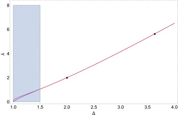
Figure 1: $\lambda$ vs $\Delta$: Blue and red colored curves are for $N=30,31$ respectively in $\det\left(M_{N\times N}\right)=0$. Two dotted points are those given by the first two polynomial solution obtained by eq. (19) and eq. (21). They are on the curve of values calculated by the Pincherle’s theorem method, showing the consistency of the two calculations.

We are only interested in the smallest positive real root of $\lambda$. We choose $N=30,31$. Notice that there are two branches in the shaded region, $1<\Delta<3/2$, which means that there is no well defined eigenvalues in this regime. We find that a good fit for the numerical result can be given by

$$\lambda\approx 1.18\Delta^{4/3}-0.97\;\;\mbox{for}\;\;3/2\leq\Delta\leq 4,$$ (16)

so that the eigenvalue is a continumous function of $\Delta$. The critical temperature can now be calculated by Eqs. (7) and (16). On the other hand, for $1<\Delta<3/2$ which is the shaded region in Figure 1, $\lambda$ hence the critical temperature is not well defined. Therefore in this paper we only consider the region $\Delta>3/2$.

IV Scaling dimension from the black hole interior

Now we come back to our main goal, the determination of the discrete values of allowed scaling dimension.

If we include the interior of the black hole as well as outside as the domain of the Heun’s equation, eq.(9) should be a polynomial, because eq.(13) shows that the infinite series is divergent at $x\geq 1$. If the degree of the polynomial is $N$, then we need to impose

$$d_{N}\neq 0,\quad d_{N+1}=d_{N+2}=0,$$ (17)

which is necessary and sufficient condition for the solution to be a degree $N$ polynomial. The equation (11) request that $\gamma_{N+1}=0$ should hold as well. Then, there are essentially two conditions for which we need to impose

$$\gamma_{N+1}=d_{N+1}=0\quad\mbox{ for degree }N\in\mathbb{N}_{0},$$ (18)

because in this case $d_{N+2}=0$ iff $\gamma_{N+1}=0$ under the assumption of $d_{N+1}=0$. Notice that since all $d_{n}$ are functions of the parameters in the differential equation, there should be at least two parameters which can be fine tuned to satisfy above two conditions. This means that in our case there are two parameters which should be quantized. We call them ’eigenvalues’. We remind the readers that for the hypergeometric case which has only three singularities at $0,1,\infty$, the recurrence equations involve only two terms ($d_{n}$ , $d_{n+1}$) after factoring out the solution’s behaviors near the singularities at the zero and infinity, and we only need to impose $d_{N+1}=0$ which gives us quantization of one parameter, the energy in Schroedinger equation for example. For the system with more than three singularities, we meet three or more term recurrence relation, which is our case.

Now coming back to our case, if the equations contains exactly two parameters, they are generically quantized, because the solutions corresponds to the intersection points of the two curves defined by eqs.(18). In our case, we have $\lambda$ and $\Delta$ and these parameters are quantized. More explicitly, from eq.(12), $B_{N+1}=0$ gives

$$\lambda=2N+\Delta.$$ (19)

One interesting consequence of this result is that our solution of scalar field given in (8) always has asymptotic behavior which saturate to the finite constant. That is, although $y$ is a polynomial, the scalar function itself has well defined asymptotic value at $z\to\infty$.. It happened to be finite although we never requested its finiteness.

$$\Psi(x\to\infty)\simeq\frac{\left<\mathcal{O}_{\Delta}\right>}{\sqrt{2}r_{h}^{\Delta}}.$$ (20)

We plot solutions $\Psi(x)$ for $N=0,1,2$ and 30 in Fig. 2. In fact, the issue of the solution of holographic superconductor inside black hole was studied in recent paper by Hartnoll et.al. [12] from the different perspective. Our result corresponds to the solution to the linearized level. Nevertheless, the oscillation and its death are the same features for large polynomial order.

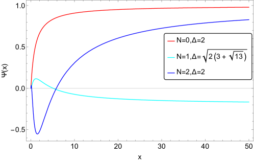
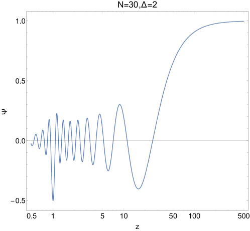
Figure 2: $\Psi(x)$ for $N=0,1,2$. Here, we set $\frac{\left<\mathcal{O}_{\Delta}\right>}{\sqrt{2}r_{h}^{\Delta}}=1$ for convenience. And $\Psi(x\to\infty)$ is finite constant. (b) N=30.

Now, $d_{N+1}=0$ gives a $N+1$-th order polynomial in $\Delta$, which we call ${\cal P}_{N+1}$, so that ${\cal P}_{N+1}(\Delta)=0$. Low-order expressions of these polynomials are given by

$$\begin{split}{\cal P}_{1}(\Delta)&=\Delta(\Delta-2),\\ {\cal P}_{2}(\Delta)&=\Delta^{4}-12\Delta^{2}-16,\\ {\cal P}_{3}(\Delta)&=(\Delta-2)(\Delta+4)(\Delta^{5}+2\Delta^{4}-36\Delta^{3}-8\Delta^{2}+256).\end{split}$$ (21)

These tell us that

$N=0$

$\Delta=2,\hbox{ and }\lambda=2,$

$N=1$

$\Delta=\sqrt{6+2\sqrt{13}},\hbox{ and }\lambda=2+\Delta.$

$N=2$

$\Delta=2,\sqrt{8\sqrt{6}+17}-1,\hbox{ and }\lambda=4+\Delta.$

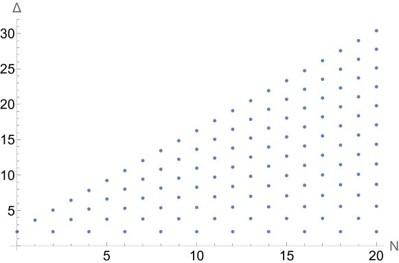
Figure 3: Allowed $\Delta$ vs $N$.

Fig. 1 shows us that above allowed values $(\Delta,\lambda)=(2,2)$ and $(3.635,5.635)$ as $N=0,1$ are placed on the line of the $\Delta,\lambda$, which would be obtained by Pincherle’s method when we request that the solution is well defined only outside the black hole. We remark that we did not set $m^{2}_{\Phi}=-2$ to get $\Delta=2$. Our method can be regarded as a calculational tool for $\Delta$. Also, notice that on the allowed points are on the curve obtained in the previous section. See the black dots in Fig. 1. Fig. 3 shows us all $\Delta$’s up to $N=20$. Due to the relation (19), lower $\Delta$ and lower $N$ solotions are more stable under the perturbation since they give lower eigenvalue $\lambda$.

V Regularity conditions

In the presence of the black hole, we often imposes contraints by requesting that the differential equation is well defined at the horizon. Then it is an urgent question whether such regularity constraints imposes further quantization condition. We will show below that this is not the case.

We consider the differential equation such as

$$E^{\prime\prime}(z)+\sum_{j=0}^{k}\frac{\rho_{j}}{z-b_{j}}E^{\prime}(z)+\sum_{j=0}^{k}\frac{w_{j}}{z-b_{j}}E(z)=0,$$ (22)

with $\sum_{j=0}^{k}w_{j}=0$. We set $b_{0}=0$ for the ease of the analysis. The case $k=2$ is the Heun’s equation. The regularity conditions at three singularities at finite positions are

$$\begin{cases}b_{1}b_{2}\left(\rho_{0}E^{\prime}(0)+E(0)w_{0}\right)=0,\cr b_{1}\left(b_{1}-b_{2}\right)\left(\rho_{1}E^{\prime}\left(b_{1}\right)+w_{1}E\left(b_{1}\right)\right)=0,\cr b_{2}\left(b_{2}-b_{1}\right)\left(\rho_{2}E^{\prime}\left(b_{2}\right)+w_{2}E\left(b_{2}\right)\right)=0.\end{cases}$$ (23)

The solution of Eq.(22) is expressible by a Frobenius series. According to Fuchs’ theorem, its radius of convergence is at least as large as the minimum of the radii of convergence of $\sum_{j=0}^{k}\frac{\rho_{j}}{z-b_{j}}$ and $\sum_{j=0}^{k}\frac{w_{j}}{z-b_{j}}$. If we require that the domain of a solution of Eq.(22) is entire complex plane or real line, the solution should be a polynomial. Suppose it is of degree $N$. After factoring out the behavior near $z=\infty$ and dividing the Eq.(22) by $E^{\prime\prime}(z)$, the following is the leading terms near $z=\infty$:

$$\Big{(}\sum_{j=1}^{2}b_{j}w_{j}+N\big{(}\sum_{j=0}^{2}\rho_{j}+N-1\big{)}\Big{)}+z\sum_{j=0}^{2}w_{j}=0.$$ (24)

The vanishing of the second term is the regularity condition which was already required in the definition of the Fuchsian equation. The first term requests :

$$\sum_{j=1}^{2}b_{j}w_{j}+N\Big{(}\sum_{j=0}^{2}\rho_{j}+N-1\Big{)}=0,$$ (25)

which is the condition for the solution to be a polynomial of degree $N$. From Eq.(23) and Eq.(25), we have 4 conditions to be satisfied. One may worry that the problem could be over determined and in general we might not have a solution. So our question is how many of these regularity conditions are automatically satisfied due to the equation of motion. We will prove that all regularity conditions are satisfied automatically by the solution of equation of motion. Therefore the regularity condition will not request any further constraint. For this we repeat the calculation in slightly more general setting.

Let $E(z)=\sum_{n=0}^{\infty}d_{n}z^{n}$ and substitute it into Eq.(22).

$$\sum_{n=0}\alpha_{n}d_{n+1}z^{n}+\sum_{n=0}\beta_{n}d_{n}z^{n}+\sum_{n=1}\gamma_{n}d_{n-1}z^{n}=0$$ (26)

with

$$\begin{cases}\alpha_{n}=b_{1}b_{2}(n+1)\left(n+\rho_{0}\right),\cr\beta_{n}=w_{0}b_{,1}^{2}-n\left((n-1)b_{,1}^{2}+b_{,1}^{2}\rho_{,0}^{2}-(b\rho)_{,1}^{2}\right),\cr\gamma_{n}=\left(b_{1}w_{1}-b_{2}w_{,0}^{1}\right)+(n-1)\left(\rho_{,0}^{2}+n-2\right),\end{cases}$$ (27)

where $b_{,1}^{2}=\sum_{j=1}^{2}b_{j}$, $\rho_{,0}^{2}=\sum_{j=0}^{2}\rho_{j}$, $(b\rho)_{,1}^{2}=\sum_{j=1}^{2}b_{j}\rho_{j}$ and $w_{,0}^{1}=\sum_{j=0}^{1}w_{j}$. Then eq.(26) becomes

$$\alpha_{0}d_{1}+\beta_{0}d_{0}+\sum_{n=1}^{\infty}\left(\alpha_{n}d_{n+1}+\beta_{n}d_{n}+\gamma_{n}d_{n-1}\right)z^{n}=0.$$ (28)

As before, for the series to teminate at $d_{N}z^{N}$, we need

$$\alpha_{0}d_{1}+\beta_{0}d_{0} =0,$$ (29)

$$\alpha_{n}d_{n+1}+\beta_{n}d_{n}+\gamma_{n}d_{n-1} =0,\hbox{ for~{} all }1\leq n$$ (30)

$$d_{N+1}=0,\quad\gamma_{N+1} =0.$$ (31)

With these, the LHS of the first regularity condition of eq.(23) is

$$b_{1}b_{2}\left(\mathit{d}_{1}\rho_{0}+\mathit{d}_{0}w_{0}\right),$$ (32)

which vanishes by the first relation of eq.(31). The LHS of the second regularity condition of eq.(23) becomes

$$\sum_{n=1}^{\infty}\left(\tilde{\alpha}_{n}\mathit{d}_{n+1}+\tilde{\beta}_{n}\mathit{d}_{n}+\tilde{\gamma}_{n}\mathit{d}_{n-1}\right)b_{1}^{n}+b_{1}b_{2}\left(\mathit{d}_{1}\rho_{0}+\mathit{d}_{0}w_{0}\right),$$ (33)

with

$$\begin{cases}\tilde{\alpha}_{n}=\alpha_{n}-b_{1}b_{2}n(n+1),\cr\tilde{\beta}_{n}=\beta_{n}+\left(b_{1}+b_{2}\right)(n-1)n,\cr\tilde{\gamma}_{n}=\gamma_{n}-(n-2)(n-1).\end{cases}$$ (34)

All terms in eq. (33) vanish due to the eq. (31). We can easily check $\tilde{\alpha}_{n}$, $\tilde{\beta}_{n}$ and $\tilde{\gamma}_{n}$ have the following relation

$$\tilde{\alpha}_{n}+\tilde{\beta}_{n+1}b_{1}+\tilde{\gamma}_{n+2}b_{1}^{2}=\alpha_{n}+\beta_{n+1}b_{1}+\gamma_{n+2}b_{1}^{2}.$$ (35)

Now, notice that

$$\sum_{n=1}\left(\tilde{\alpha}_{n}\mathit{d}_{n+1}+\tilde{\beta}_{n}\mathit{d}_{n}+\tilde{\gamma}_{n}\mathit{d}_{n-1}\right)b_{1}^{n}$$ (36)

$$=\sum_{n=1}b_{1}^{n}\mathit{d}_{n+1}\left(\tilde{\alpha}_{n}+\tilde{\beta}_{n+1}b_{1}+\tilde{\gamma}_{n+2}b_{1}^{2}\right),$$

$$+b_{1}\mathit{d}_{1}\tilde{\beta}_{1}+b_{1}^{2}\mathit{d}_{1}\tilde{\gamma}_{2}+b_{1}\mathit{d}_{0}\tilde{\gamma}_{1}$$ (37)

$$=\sum_{n=1}b_{1}^{n}\mathit{d}_{n+1}\left(\alpha_{n}+\beta_{n+1}b_{1}+\gamma_{n+2}b_{1}^{2}\right),$$

$$+\beta_{1}b_{1}\mathit{d}_{1}+b_{1}^{2}\gamma_{2}\mathit{d}_{1}+b_{1}\gamma_{1}\mathit{d}_{0},$$ (38)

$$=\sum_{n=1}\left(\alpha_{n}\mathit{d}_{n+1}+\beta_{n}\mathit{d}_{n}+\gamma_{n}\mathit{d}_{n-1}\right)b_{1}^{n}=0$$ (39)

which vanishes by the recurrence relation in eq(31). The regularity conditions at $z=b_{2}$ in eq.(23) is satisfied by $b_{1}\to b_{2}$. Finally the second equation of eq.(25) is equivalent to $\gamma_{N+1}=0$ as one can see from the expression in eq.(27). Therefore, all the 4 regularity conditions are automatically satisfied by the polynomial solutions of the equation.

VI Discussion

Our work is for AdS₅ dual to a 3+1 dimensional system. For AdS₄ blackhole, we have a technical difficulty in applying our method: while AdS₅ metric is even under the $z\to-z$ reflection, we do not have such symmetry in AdS₄. Therefore we can not reduce the singularity of the differential equation. As a consequence, the Heun’s equation leads us to a four term recurrence relation. In this case, for a solution to be valid inside the black hole, we need at least 3 parameters while we have only two.

We also would like to mention the key difference from the previous literatures. While the previous solutions request just the regularity of the solution near the horizon, we claim that the horizon regularity condition implies the regularity at the center of black hole [13].