Solving the time-optimal control problem for nonlinear non-autonomous linearizable systems

Abstract

We present the conditions under which the time-optimal control problem for a nonlinear non-autonomous linearizable system can be solved by the method of successive approximations, at each step of which a power Markov moment min-problem is solved. The proposed method can be efficiently implemented by use of symbolic and numerical calculations.

Keywords: Nonlinear control system, Linearizablity problem, Linear control system with analytic matrices, Method of successive approximations, power Markov moment min-problem with gaps.

MSC2020: 93B18, 93C10, 49K30, 49M99.

1 Introduction

The linearizability problem is an important issue for nonlinear control theory. For nonlinear systems that turn out to be linearizable, well-developed methods of linear control theory can be applied. In this paper, we propose a method for solving the time-optimal control problem for non-autonomous linearizable systems with a single input.

Let us consider a control system

$$\dot{x}=f(t,x,u),\ \ x\in{\mathbb{R}}^{n},\ u\in{\mathbb{R}}^{1},$$ (1.1)

and suppose that $f\in C^{1}((-\delta,\delta)\times U(0)\times{\mathbb{R}})$ where $\delta>0$ and $U(0)\subset{\mathbb{R}}^{n}$ is a neighborhood of the origin. We say that the system (1.1) is locally analytically linearizable at the origin if there exists a neighborhood $(-\delta^{\prime},\delta^{\prime})\times U^{\prime}(0)\subset(-\delta,\delta)\times U(0)$ and a local change of variables $z=F(t,x)\in C^{2}((-\delta^{\prime},\delta^{\prime})\times U^{\prime}(0))$ such that the system in the new variables is linear, i.e., takes the form

$$\dot{z}=A(t)z+b(t)u,$$ (1.2)

where components of $A(t)$ and $b(t)$ are real analytic in $(-\delta^{\prime},\delta^{\prime})$. Here and below under ‘‘local change of variables’’ we mean a map $F(t,x)$ which takes the origin to itself and is locally invertible w.r.t. $x$, i.e.,

$$F(t,0)\equiv 0,\ \ \det F_{x}(t,x)\neq 0,\ \ (t,x)\in(-\delta^{\prime},\delta^{\prime})\times U^{\prime}(0),$$

where the sub-index means the derivative in $x$, i.e., $F_{x}(t,x)=\frac{\partial F(t,x)}{\partial x}$. Clearly, this is true (maybe in a smaller neighborhood) if $\det F_{x}(0,0)\neq 0$.

The linearizability property can be used for solving the local controllability problem for the system (1.1): for two given points $x(0)=x^{0}$, $x(T)=x^{1}$, find $z^{0}=F(0,x^{0})$ and $z^{1}=F(T,x^{1})$ and then find a control $u(t)$ which steers the linear system (1.2) from $z^{0}$ to $z^{1}$ in the time $T$; then this control steers the system (1.1) from $x^{0}$ to $x^{1}$. In this paper we propose a method for solving the time-optimal control problem under the constraint $|u(t)|\leq 1$.

First of all, an efficient method of solving the linear time-optimal control problem should be involved. In Subsection 2.1 we recall known results related to systems of the form (1.2), where $A(t)$ and $b(t)$ are real analytic in a neighborhood of zero. For start points from a neighborhood of the origin, an optimal control equals $\pm 1$ and has no more than $n-1$ switchings. The direct substitution of such a control leads to a system of $n$ nonlinear equations with $n$ unknowns (switching times and the optimal time). However, under some conditions, the optimal control can be found by the method of successive approximations, at each step of which a power Markov moment min-problem with gaps is solved. The power Markov moment problem was originated in [1], a deep discussion can be found in [2]. The statement of the Markov moment min-problem and its application to the time-optimal control problem was proposed in [3], [4]; in many cases it admits an effective solution.

Then, in Subsection 2.2, we recall some recent results on linearizability conditions for non-autonomous systems proposed in [5]. Additionally to linearizability conditions known since [6], [7] and generalized to systems of the class $C^{1}$ in [8], [9], in the non-autonomous case some new conditions arise, see [10] and [11] for further discussion.

Finally, in Section 3 we combine the known results mentioned above and formulate the main result of the paper (Theorem 3), which gives a method for solving the time-optimal control problem for non-autonomous linearizable systems. This method can be effectively used for numerical application; we demonstrate it by an illustrative example in Section 4.

2 Background

2.1 Solving the time-optimal control problem for linear non-autonomous system

Consider a control system of the form

$$\dot{x}=A(t)x+b(t)u,$$ (2.1)

where the matrix $A(t)$ and the vector $b(t)$ are real analytic in a neighborhood of zero. Denote

$$\textstyle L_{i}=\frac{1}{i!}\left(-A(t)+\frac{d}{dt}\right)^{i}b(t)|_{t=0},\ \ i\geq 0,$$

and suppose

$${\mathrm{rank}}\{L_{i}\}_{i=0}^{\infty}=n.$$ (2.2)

Let $k_{1},\ldots,k_{n}$ be the indices of the first $n$ linearly independent vectors from the sequence $\{L_{i}\}_{i=0}^{\infty}$. Denote

$$L=(-L_{k_{1}},\ldots,-L_{k_{n}}).$$

The condition (2.2) implies that the system (2.1) is locally controllable in a neighborhood of the origin. Let $u(t)$ be a control that steers a point $x^{0}$ from this neighborhood to the origin, i.e.,

$$\dot{x}=A(t)x+b(t)u(t),\ \ x(0)=x^{0},\ \ x(\theta)=0.$$

Then

$$x^{0}=-\int_{0}^{\theta}\Phi^{-1}(t)b(t)u(t)dt=-\sum_{j=0}^{\infty}L_{j}\int_{0}^{\theta}t^{j}u(t)dt,$$ (2.3)

where the matrix $\Phi(t)$ is such that $\dot{\Phi}(t)=A(t)\Phi(t)$, $\Phi(0)=I$. This means that the right hand side of (2.3) is a series of power moments of the function $u(t)$ with vector coefficients $L_{j}$. Equality (2.3) implies

$$(L^{-1}x^{0})_{i}=\int_{0}^{\theta}t^{k_{i}}u(t)dt+\sum_{j=k_{i}+1}^{\infty}\alpha_{ji}\int_{0}^{\theta}t^{j}u(t)dt,\ \ i=1,\ldots,n,$$ (2.4)

where $\alpha_{ji}$ are components of the vector $-L^{-1}L_{j}$. Below we suppose $|u(t)|\leq 1$, then $|\int_{0}^{\theta}t^{j}u(t)dt|\leq\frac{1}{j+1}\theta^{j+1}$. This means that locally, for small $\theta$, the first term in the right hand side of (2.4) is a ‘‘leading’’ one. Having this in mind, we consider the power Markov moment min-problem with gaps [3], [4], [12]

$$y_{i}=\int_{0}^{\theta}t^{k_{i}}u(t)dt,\ \ i=1,\ldots,n,\ \ |u(t)|\leq 1,\ \ \theta\to\min.$$ (2.5)

As was shown in [13], the solution $(\widehat{\theta}(x^{0}),\widehat{u}(t;x^{0}))$ of the time-optimal control problem

$$\dot{x}=A(t)x+b(t)u,\ \ x(0)=x^{0},\ x(\theta)=0,\ \ |u(t)|\leq 1,\ \ \theta\to\min$$ (2.6)

and the solution $(\theta(y),u(t;y))$ of the power Markov moment min-problem (2.5) for ${y=L^{-1}x^{0}}$ are equivalent at the origin, i.e.,

$$\frac{\widehat{\theta}(x^{0})}{\theta(L^{-1}x^{0})}\to 1,\ \ \frac{1}{\theta}\int_{0}^{\theta}|\widehat{u}(t;x^{0})-u(t;L^{-1}x^{0})|dt\to 0\ \ \mbox{ as }\ \ x^{0}\to 0.$$

Under some additional conditions this result can be strengthened, namely, a fixed-point iteration can be used for finding the solution [4]. In [13], the following theorem was proved.

Theorem 1.

Consider the system (2.1) where $A(t)$ and $b(t)$ are real analytic in a neighborhood of zero and assume the condition (2.2) holds. Suppose also that

$$L_{i}=0\ \ \mbox{for all}\ \ i<k_{n}\ \mbox{such that}\ i\neq k_{j},\ j=1,\ldots,n-1.$$ (2.7)

Then there exists a neighborhood $U(0)$ of the origin such for any $x^{0}\in U(0)$ the solution $(\widehat{\theta}(x^{0}),\widehat{u}(t;x^{0}))$ of the time-optimal control problem (2.6) can be found as

$$\widehat{\theta}(x^{0})=\lim_{r\to\infty}\theta(y^{r}),\ \ \widehat{u}(t;x^{0})=\lim_{r\to\infty}u(t;y^{r}),$$ (2.8)

where $(\theta(y),u(t;y))$ denotes the solution of the Markov moment min-problem (2.5) and the sequence $\{y^{r}\}_{r=0}^{\infty}$ is defined recursively as

$$y^{0}=L^{-1}x^{0},\ \ y^{r+1}=L^{-1}\left(x^{0}+\int_{0}^{\theta(y_{r})}\Phi^{-1}(t)b(t)u(t;y^{r})dt\right)+y^{r},\ \ r\geq 0.$$

This result follows from the fact that under the condition (2.7) the map

$$y\mapsto L^{-1}\left(x^{0}+\sum_{j\neq k_{i}}L_{j}\int_{0}^{\theta(y)}t^{j}u(t;y)dt\right)$$

is a contraction in a neighborhood of the origin; if $\bar{y}$ is its fixed point, then $(\widehat{\theta}(x^{0}),\widehat{u}(t;x^{0}))=(\theta(\bar{y}),u(t;\bar{y}))$.

In particular, if $k_{i}=i-1$, $i=1,\ldots,n$, then the condition (2.7) is satisfied automatically. Moreover, in this case the moment problem (2.5) has no gaps, hence, it can be effectively and completely solved by the method described in [3]; see also [14] for additional comments and examples.

For the power Markov moment min-problem with gaps (2.5) of the general form, a deep study was obtained in [12]. One particular case of even gaps was treated in [15].

2.2 Conditions of linearizability for non-autonomous systems

In [5], linearizability conditions for nonlinear non-autonomous control systems were given; further analysis can be found in [10], [11]. In this subsection we formulate a direct corollary of these results related to a local statement of the problem.

First, let us notice that if a system of the form (1.1) is locally linearizable, then it is of the affine form

$$\dot{x}=a(t,x)+b(t,x)u,\ \ a(t,0)\equiv 0,$$ (2.9)

where the condition $a(t,0)\equiv 0$ means that the origin is an equilibrium of the system. Denote by ${\mathcal{R}}$ the following operator which acts on a vector function $c(t,x)$ by the rule

$${\mathcal{R}}c(t,x)=c_{t}(t,x)+c_{x}(t,x)a(t,x)-a_{x}(t,x)c(t,x),$$

where sub-indices $t$ and $x$ denote the derivatives w.r.t. $t$ and $x$ respectively. Introduce the following matrix

$$R(t,x)=(b(t,x),{\mathcal{R}}b(t,x),\ldots,{\mathcal{R}}^{n-1}b(t,x)).$$

By $[\cdot,\cdot]$ we denote the Lie bracket, $[c(t,x),d(t,x)]=d_{x}(t,x)c(t,x)-c_{x}(t,x)d(t,x)$. Also we use the notation $k^{\underline{j}}$ for the falling factorial,

$$k^{\underline{j}}=k(k-1)\cdots(k-j+1),\ j\geq 1,\ \ \ k^{\underline{0}}=1.$$

Theorem 2.

Consider an affine non-autonomous control system of the form (2.9), where $a(t,x)\in C^{2}((-\delta,\delta)\times U(0))$, $b(t,x)\in C^{1}((-\delta,\delta)\times U(0))$. This system is locally linearizable if and only is all vector functions ${\mathcal{R}}^{i}b(t,x)$ for $1\leq i\leq n$ exist and belong to the class $C^{1}((-\delta,\delta)\times U(0))$ and the following conditions are satisfied,

1. $[{\mathcal{R}}^{i}b(t,x),{\mathcal{R}}^{j}b(t,x)]=0$ for $0\leq i<j\leq n-1$, $(t,x)\in(-\delta,\delta)\times U(0)$;

2. ${\mathrm{rank}}R(t,x)=n$ for $t\in(-\delta,0)\cup(0,\delta)$ and $x\in U(0)$;

3. the vector function $R^{-1}(t,x){\mathcal{R}}^{n}b(t,x)$ depends only on $t$, i.e.,

   $$R^{-1}(t,x){\mathcal{R}}^{n}b(t,x)=\gamma(t);$$

4. components of $\gamma(t)$ are analytic or meromorphic functions in a neighborhood of the point $t=0$ with a pole at $t=0$ such that

   $$\gamma_{i}(t)=\sum_{j=-n+i-1}^{\infty}\gamma_{i,j}t^{j},\ \ i=1,\ldots,n,$$

   the indicial equation

   $$k^{\underline{n}}-\sum_{s=1}^{n}k^{\underline{n-s}}\gamma_{n-s+1,-s}=0$$

   has $n$ integer nonnegative roots $0\leq k_{1}<\cdots<k_{n}$ and

   $${\mathrm{rank}}\begin{pmatrix}V_{k_{1}+1,k_{1}}&V_{k_{1}+1,k_{1}+1}&0&\cdots&0\\ \cdots&\cdots&\cdots&\cdots&\cdots\\ V_{k_{n},k_{1}}&V_{k_{n},k_{1}+1}&V_{k_{n},k_{1}+2}&\cdots&V_{k_{n},k_{n}-1}\end{pmatrix}=k_{n}-k_{1}-n+1,$$ (2.10)

   where

   $$\begin{array}[]{l}\displaystyle V_{k,k}=k^{\underline{n}}-\sum_{s=1}^{n}k^{\underline{n-s}}\gamma_{n-s+1,-s},\\ \displaystyle V_{k,j}=-\sum_{s=1}^{n}j^{\underline{n-s}}\gamma_{n-s+1,k-j-s},\ \ j\leq k-1.\end{array}$$

Remark 1.

Conditions 1 and 2 of Theorem 3 are analogous to linearizability conditions for autonomous systems as well as the requirements ${\mathcal{R}}^{k}b(t,x)\in C^{1}((-\delta,\delta)\times U(0))$, $k=0,\ldots,n$ [8]. Conditions 3 and 4 are specific for non-autonomous case [5], [11]. Condition $a(t,x)\in C^{2}((-\delta,\delta)\times U(0))$ is of technical character, see [10] for a detailed discussion.

Remark 2.

If the system (2.9) is linearizable, its linear representation (1.2) is not unique. It is convenient to choose it in a driftless form

$$\dot{z}=g(t)u,$$ (2.11)

which can be considered as a canonical form for linear systems suitable both for autonomous and non-autonomous cases. Components of $g(t)$ can be found as $n$ linearly independent real analytic solutions of the differential equation

$$w^{(n)}=\sum_{k=1}^{n}\gamma_{k}(t)w^{(k-1)},$$ (2.12)

where $w^{(j)}$ denotes the $j$-th derivative in $t$. If the analytic solving of the differential equation (2.12) is impossible, one can find sufficiently many coefficients of the Taylor series for a solution using the recurrent formula

$$w_{k}=-\frac{1}{V_{k,k}}\sum_{j=0}^{k-1}V_{k,j}w_{j},\ \ k\geq 0,\ k\neq k_{i},\ i=1,\ldots,n,$$ (2.13)

where $w_{k_{1}},\ldots,w_{k_{n}}$ are arbitrary.

It is convenient to choose $g_{i}(t)$ such that $g_{i}(t)=-t^{k_{i}}+o(t^{k_{n}})$; in this case $L=I$. When using (2.13), one should choose $w_{k_{i}}=-1$ and $w_{k_{j}}=0$ for $j\neq i$.

Remark 3.

A change of variables $F(t,x)$ satisfies the following partial differential equations

$$F_{t}(t,x)+F_{x}(t,x)a(t,x)=0,\ F_{x}(t,x){\mathcal{R}}^{k}b(t,x)=g^{(k)}(t),\ \ k\geq 0.$$

It is more convenient to find it as a solution of the system

$$F_{x}(t,x)=G(t)R^{-1}(t,x),\ F_{t}(t,x)=-F_{x}(t,x)a(t,x),$$ (2.14)

where $G(t)=(g(t),\dot{g}(t),\ldots,g^{(n-1)}(t))$; see also Remark 4 below.

3 Main result

Now we combine the theorems formulated in the previous section and present our main result.

Theorem 3.

Suppose that the system (2.9) satisfies the conditions of Theorem 2 and, additionally,

$$V_{\ell,k_{i}}=0\ \ \mbox{ for }\ \ \ell=k_{i}+1,\ldots,k_{n},\ \ i=1,\ldots,n-1.$$ (3.1)

Then there exist $\delta^{\prime}>0$, a neighborhood $U^{\prime}(0)$ of the origin and a local change of variables $z=F(t,x)\in C^{2}((-\delta^{\prime},\delta^{\prime})\times U^{\prime}(0))$ such that for any $x^{0}\in U^{\prime}(0)$ the solution $(\widehat{\theta}(x^{0}),\widehat{u}(t;x^{0}))$ of the time-optimal control problem

$$\dot{x}=a(t,x)+b(t,x)u,\ x(0)=x^{0},\ x(\theta)=0,\ |u(t)|\leq 1,\ \theta\to\min$$

can be found by the method of successive approximations as (2.8), where

$$y^{0}=L^{-1}F(0,x^{0}),\ \ y^{r+1}=L^{-1}\left(F(0,x^{0})+\int_{0}^{\theta(y_{r})}g(t)u(t;y^{r})dt\right)+y^{r},\ \ r\geq 0.$$ (3.2)

Here components of $g(t)$ are $n$ linearly independent analytic solutions of the differential equation (2.12), $L=(-\frac{1}{k_{1}!}g^{(k_{1})}(0),\ldots,-\frac{1}{k_{n}!}g^{(k_{n})}(0))$, the vector function $F(t,x)$ satisfies the system of differential equations (2.14) and $F(0,0)=0$.

Proof.

We notice that the condition (3.1) obviously implies (2.10).

To prove the theorem, it is sufficient to show that (3.1) implies (2.7). However, it easily follows from the recurrent formula (2.13). ∎

Remark 4.

To apply Theorem 3, it is not necessary to solve the system (2.14). In fact, we only need to find $F(0,x^{0})$, so we can proceed as follows. Denote $M(x)=G(t)R^{-1}(t,x)|_{t=0}$ and, for any $k=1,\ldots,n$, consider the equations

$$\frac{\partial F_{k}(0,x)}{\partial x_{s}}=M_{ks}(x),\ \ s=1,\ldots,n.$$

Successively for $s=1,\ldots,n$, solve (at least, numerically) the Cauchy problem for a single ordinary differential equation

$$z^{\prime}(\tau)=M_{ks}(0,x_{1}^{0},\ldots,x^{0}_{s-1},\tau,0,\ldots,0),\ \ z(0)=F_{k}(0,x_{1}^{0},\ldots,x^{0}_{s-1},0,\ldots,0),$$

then $F_{k}(0,x_{1}^{0},\ldots,x^{0}_{s-1},x^{0}_{s},0,\ldots,0)=z(x_{s}^{0})$. We find $F_{k}(0,x^{0})$ after $n$ such steps.

4 Example

As an illustrative example, we consider the following system

$$\begin{array}[]{l}\dot{x}_{1}=u,\\ \dot{x}_{2}=(t-{\textstyle\frac{1}{3}}t^{4}-2x_{1}x_{3}-(2t^{2}+t^{3}+{\textstyle\frac{1}{5}}t^{5})x_{1}^{2})u,\\ \dot{x}_{3}=(t^{3}+{\textstyle\frac{1}{5}}t^{3}-t^{2})u-2tx_{1}.\end{array}$$ (4.1)

Let us check the conditions of Theorem 3. We have

$$a(t,x)=\begin{pmatrix}0\\ 0\\ -2tx_{1}\end{pmatrix},\ \ b(t,x)=\begin{pmatrix}1\\ t-{\textstyle\frac{1}{3}}t^{4}-2x_{1}x_{3}-(2t^{2}+t^{3}+{\textstyle\frac{1}{5}}t^{5})x_{1}^{2}\\ t^{3}+{\textstyle\frac{1}{5}}t^{5}-t^{2}\end{pmatrix},$$

$${\mathcal{R}}b(t,x)=\begin{pmatrix}0\\ 1-{\textstyle\frac{4}{3}}t^{3}-(3t^{2}+t^{4})x_{1}^{2}\\ 3t^{2}+t^{4}\end{pmatrix},\ \ {\mathcal{R}}^{2}b(t,x)=\begin{pmatrix}0\\ -4t^{2}-(6t+4t^{3})x_{1}^{2}\\ 6t+4t^{3}\end{pmatrix},$$

$$R(t,x)=(b(t,x),{\mathcal{R}}b(t,x),{\mathcal{R}}^{2}b(t,x)),\ \ \ {\mathcal{R}}^{3}b(t,x)=\begin{pmatrix}0\\ -8t-(6+12t^{2})x_{1}^{2}\\ 6+12t^{2}\end{pmatrix}.$$

First, we notice that $\det R(t,x)=6t+4t^{3}+4t^{4}-{\textstyle\frac{4}{3}}t^{6}$, hence, $R(t,x)$ is nonsingular at points $(t,x)$ from some neighborhood of the origin such that $t\neq 0$. Then, we find that $[b(t,x),{\mathcal{R}}b(t,x)]=[b(t,x),{\mathcal{R}}^{2}b(t,x)]=[{\mathcal{R}}b(t,x),{\mathcal{R}}^{2}b(t,x)]=0$, therefore, conditions 1 and 2 of Theorem 2 hold.

Further,

$$R^{-1}(t,x){\mathcal{R}}^{3}b(t,x)=\begin{pmatrix}0\\[2.0pt] \frac{12t(2t^{2}-3)}{9+6t^{2}+6t^{3}-2t^{5}}\\[6.0pt] \frac{3(3+6t^{2}+8t^{3}-4t^{5})}{t(9+6t^{2}+6t^{3}-2t^{5})}\end{pmatrix}=\begin{pmatrix}\gamma_{1}(t)\\ \gamma_{2}(t)\\ \gamma_{3}(t)\end{pmatrix},$$

where $\gamma_{i}(t)$ are analytic or meromorphic and $\gamma_{1}(t)=0$, $\gamma_{2}(t)=-4t+O(t^{3})$, $\gamma_{3}(t)=\frac{1}{t}+O(t)$. Hence, the indicial equation is

$$k^{\underline{3}}-k^{\underline{2}}\gamma_{3,-1}-k^{\underline{1}}\gamma_{2,-2}-k^{\underline{0}}\gamma_{1,-3}=0;$$

since $\gamma_{1,-3}=0$, $\gamma_{2,-2}=0$, $\gamma_{3,-1}=1$, it takes the form

$$k(k-1)(k-2)-k(k-1)=0$$

and has the roots $k_{1}=0$, $k_{2}=1$, $k_{3}=3$. Now,

$$V_{1,0}=-\gamma_{1,-2}=0,\ \ V_{2,0}=-\gamma_{1,-1}=0,\ \ V_{3,0}=-\gamma_{1,0}=0,$$

$$V_{2,1}=-\gamma_{2,-1}-\gamma_{1,-2}=0,\ V_{3,1}=-\gamma_{2,0}-\gamma_{1,-1}=0,$$

hence, conditions 3 and 4 of Theorem 2 and the condition (3.1) are satisfied. Hence, the system (4.1) is locally linearizable and the time-optimal control problem for this system can be solved by the method of successive approximations.

We find a system after linearization in the driftless form (2.11), where the components of $g(t)$ are solutions of the following differential equation

$$w^{\prime\prime\prime}=\gamma_{1}(t)w+\gamma_{2}(t)w^{\prime}+\gamma_{3}(t)w^{\prime\prime}.$$

In our case, we have

$$t(9+6t^{2}+6t^{3}-2t^{5})w^{\prime\prime\prime}=12t^{2}(2t^{2}-3)w^{\prime}+3(3+6t^{2}+8t^{3}-4t^{5})w^{\prime\prime},$$

and it is easy to check that $g_{1}(t)=-1$, $g_{2}(t)=-t+\frac{1}{3}t^{4}$ and $g_{3}(t)=-t^{3}-\frac{1}{5}t^{5}$ are its three linearly independent solutions. Hence, $L=I$ and in the new coordinates the system takes the driftless form

$$\begin{array}[]{l}\dot{z}_{1}=-u,\\ \dot{z}_{2}=-(t-{\textstyle\frac{1}{3}}t^{4})u,\\ \dot{z}_{3}=-(t^{3}+{\textstyle\frac{1}{5}}t^{5})u.\end{array}$$

In this case, the power Markov moment min-problem (2.5) is of the form

$$y_{1}=\int_{0}^{\theta}u(t)dt,\ y_{2}=\int_{0}^{\theta}t\,u(t)dt,\ y_{3}=\int_{0}^{\theta}t^{3}u(t)dt,\ \ |u(t)|\leq 1,\ \theta\to\min.$$ (4.2)

Its solution can be found directly. In fact, the optimal control is unique and equals $\pm 1$ and has no more than two switchings. Since the set of points for which it has less than two switchings is of zero measure, for numerical float-point calculation it is sufficient to assume that there are exactly two switchings; denote them by $t_{1}$ and $t_{2}$, and let $\theta$ be the optimal time. Then

$$\begin{array}[]{l}\pm y_{1}=-2t_{1}+2t_{2}-\theta,\\ \pm y_{2}=-t_{1}^{2}+t_{2}^{2}-\frac{1}{2}\theta^{2},\\ \pm y_{3}=-\frac{1}{2}t_{1}^{4}+\frac{1}{2}t_{2}^{4}-\frac{1}{4}\theta^{4},\end{array}$$

where the upper (resp., lower) sign means that $u(t)$ equals $+1$ (resp, $-1$) on the first and the third intervals of constancy. Let us denote $c_{1}^{\pm}=\frac{1}{2}(\pm y_{1}+\theta)$, $c_{2}^{\pm}=\pm y_{2}+\frac{1}{2}\theta^{2}$, $c_{3}=2(\pm y_{3}+\frac{1}{4}\theta^{4})$, then

$$t_{2}-t_{1}=c_{1}^{\pm},\ \ t_{2}^{2}-t_{1}^{2}=c_{2}^{\pm},\ \ t_{2}^{4}-t_{1}^{4}=c_{3}^{\pm}.$$

Excluding $t_{1}$ and $t_{2}$, we get two equations w.r.t. $\theta$

$$2c_{3}^{\pm}(c_{1}^{\pm})^{2}=(c_{2}^{\pm})^{3}+c_{2}^{\pm}(c_{1}^{\pm})^{4};$$

they are polynomial equations in $\theta$ of degree 6. There exists a unique root $\theta$ of one of these equations such that $0<t_{1}<t_{2}<\theta$. Hence, it it easy to find the solution of (4.2) numerically for any $y$.

Finally, let us find $F(0,x^{0})$. We have

$$M(x)=G(t)R^{-1}(t,x)=\begin{pmatrix}-1&0&0\\ -2x_{1}x_{3}&-1&-x_{1}^{2}\\ 0&0&-1\end{pmatrix}.$$

Hence, $\frac{\partial F_{1}(0,x)}{\partial x_{1}}=-1$, $\frac{\partial F_{1}(0,x)}{\partial x_{2}}=\frac{\partial F_{1}(0,x)}{\partial x_{3}}=0$, therefore, $F_{1}(0,x^{0})=-x_{1}^{0}$. Analogously, $F_{3}(0,x^{0})=-x^{0}_{3}$. For $F_{2}(0,x)$, we have $\frac{\partial F_{2}(0,x)}{\partial x_{1}}=-2x_{1}x_{3}$, $\frac{\partial F_{1}(0,x)}{\partial x_{2}}=-1$, $\frac{\partial F_{1}(0,x)}{\partial x_{3}}=-x_{1}^{2}$. In this particular case the solution is obvious. However, we demonstrate the method of finding $F_{2}(0,x^{0})$ described in Remark 4.

Since $F(0,0,0,0)=0$, solving the Cauchy problem $z^{\prime}(\tau)=F_{2}(0,0,0,0)=0$, $z(0)=0$ we get $z(x_{1}^{0})=F_{2}(0,x^{0}_{1},0,0)=0$. Then, considering the Cauchy problem $z^{\prime}(\tau)=-1$, $z(0)=0$, we get $z(x_{2}^{0})=F_{2}(0,x_{1}^{0},x_{2}^{0},0)=-x_{2}^{0}$. Finally, solving the Cauchy problem $z^{\prime}(\tau)=-(x_{1}^{0})^{2}$, $z(0)=-x_{2}^{0}$, we get $z(x_{3}^{0})=F_{2}(0,x^{0})=-x_{2}^{0}-(x_{1}^{0})^{2}x_{3}^{0}$. As a result, $F(0,x^{0})=(-x_{1}^{0},-x_{2}^{0}-(x_{1}^{0})^{2}x_{3}^{0},-x_{3}^{0})$.

Suppose we solve the time-optimal control problem for the system (4.1) from the point $x^{0}=(-0.4,-0.2,0.1)$, then $y^{0}=F(0,x^{0})=(0.4,0.184,-0.1)$. Using the method of successive approximations we get $\lim\limits_{r\to\infty}y^{r}\approx(0.4,0.1457,-0.0714)$ and $t_{1}\approx 0.1251$, $t_{2}\approx 0.8740$, $\theta\approx 1.0978$. After 45 iterations one achieves $\|y^{r+1}-y^{r}\|<10^{-8}$; the trajectory components are shown in Fig. 1 (a).

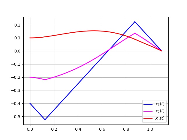
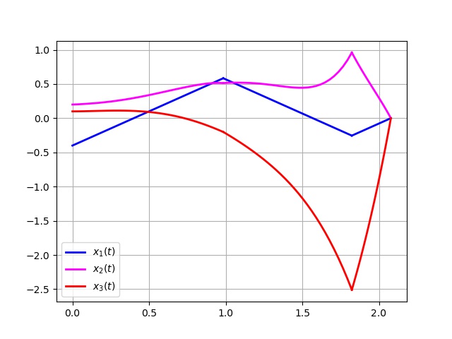
(a)                                                                    (b)

Figure 1: Components of the optimal trajectory: (a) ${x^{0}=(-0.4,-0.2,0.1)}$; (b) ${x^{0}=(-0.4,0.2,0.1)}$.

If the starting point for the initial system is $x^{0}=(-0.4,0.2,0.1)$, we get $y^{0}=(0.4,-0.216,-0.1)$ and the method of successive approximations diverges. However, one can apply the following modification: instead of (3.2), use the formula

$$y^{0}=L^{-1}F(0,x^{0}),\ \ y^{r+1}=cL^{-1}\left(F(0,x^{0})+\int_{0}^{\theta(y_{r})}g(t)u(t;y^{r})dt\right)+y^{r},\ \ r\geq 0,$$

where $c\in(0,1)$ (recall that in our example $L=I$). One can show that the mapping leading to this recursive formula is also a contraction. Though the contraction constant is greater, a domain where the method converges can be wider. So, in the previous example, if $c=\frac{1}{4}$, then $y^{r}$ converges; after 120 iterations one achieves $\|y^{r+1}-y^{r}\|<10^{-8}$. We obtain $t_{1}\approx 1.8232$, $t_{2}\approx 2.0779$, $\theta\approx 0.9843$; the trajectory components are shown in Fig. 1 (b).

References

• [1] Markov A. A. New applications of continuous fractions (Russian), Notes of the Imperial Academy of Sci. III (1896) 1–50, translation: A. Markoff, Nouvelles applications des fractions continues, Mathematische Annalen 47 (1896) 579–597.
• [2] Kreĭn M. G., Nudel’man A. A. The Markov moment problem and extremal problems. Ideas and problems of P. L. Čebyšev and A. A. Markov and their further development (Russian), Nauka, Moscow, 1973, translation: Translations of Mathematical Monographs, vol. 50. American Mathematical Society, Providence, R.I., 1977.
• [3] Korobov V. I., Sklyar G. M. Time optimality and the power moment problem (Russian), Mat. Sb. (N.S.) 134(176) (1987) 186–206, translation: Math. USSR-Sb. 62 (1989) 185-206.
• [4] Korobov V. I., Sklyar G. M. The Markov moment min-problem and time optimality (Russian), Sibirsk. Mat. Zh. 32 (1991) 60–71, translation: Siberian Math. J. 32(1991) 46-55.
• [5] Sklyar K. On mappability of control systems to linear systems with analytic matrices, Systems Control Lett. 134 (2019) 104572.
• [6] Krener A. On the equivalence of control systems and the linearization of non-linear systems. SIAM. J. Control 11 (1973) 670-676.
• [7] Jakubczyk B., Respondek W. On linearization of control systems. Bull. Acad. Sci. Polonaise Ser. Sci. Math. 28 (1980) 517–522.
• [8] Sklyar G. M., Sklyar K. V., Ignatovich S. Yu. On the extension of the Korobov’s class of linearizable triangular systems by nonlinear control systems of the class $C^{1}$. Systems Control Lett. 54 (2005) 1097–1108.
• [9] Sklyar K. V., Ignatovich S. Y., Skoryk V. O. Conditions of linearizability for multicontrol systems of the class C1. Commun. Math. Anal. 17 (2014) 359–365.
• [10] Sklyar K., Ignatovich S. On linearizability conditions for non-autonomous control systems. Advances in Intelligent Systems and Computing 196 (2020) AISC, 625–637.
• [11] Sklyar K., Ignatovich S. Invariants of linear control systems with analytic matrices and the linearizability problem. J. Dynamical and Control Systems (2021).
• [12] Korobov V. I., Sklyar G. M. Markov power min-moment problem with periodic gaps. J. of Mathematical Sciences 80 (1996) 1559–1581.
• [13] Sklyar G. M., Ignatovich S. Yu. A classification of linear time-optimal control problems in a neighborhood of the origin. J. Math. Anal. Appl. 203 (1996) 791–811.
• [14] Korobov V. I., Sklyar G. M., Ignatovich S. Yu. Solving of the polynomial systems arising in the linear time-optimal control problem. Commun. Math. Anal. Conf. 3 (2011) 153–171.
• [15] Korobov V. I., Bugaevskaya A. N. The solution of one time-optimal problem on the basis of the Markov moment min-problem with even gaps. Matematicheskaya Fizika, Analiz, Geometriya 10 (2003), 505–523.