Initiation of Alfvénic turbulence by Alfven wave collisions: a numerical study

In the framework of compressional magnetohydrodynamics (MHD), we study numerically the commonly accepted presumption that the Alfvénic turbulence is generated by the collisions between counter-propagating Alfvén waves (AWs). In the conditions typical for the low-beta solar corona and inner solar wind, we launch in the three-dimensional simulation box two counter-propagating AWs and analyze polarization and spectral properties of perturbations generated before and after AW collisions. The observed post-collisional perturbations have different polarization and smaller cross-field scales than the original waves, which supports theoretical scenarios with direct turbulent cascades. However, contrary to theoretical expectations, the spectral transport is strongly suppressed at the scales satisfying the classic critical balance of incompressional MHD. Instead, a modified critical balance can be established by colliding AWs with significantly shorter perpendicular scales. We discuss consequences of these effects for the turbulence dynamics and turbulent heating of compressional plasmas. In particular, solar coronal loops can be heated by the strong turbulent cascade if the characteristic widths of the loop sub-structures are more than 10 times smaller than the loop width. The revealed new properties of AW collisions have to be incorporated in the theoretical models of AW turbulence and related applications.

1 Introduction

Recent studies have revealed that the turbulence in magnetized plasmas is greatly affected by the Alfvén wave effects. The well-documented example is the solar-wind turbulence whose nature is essentially Alfvénic and turbulent fluctuations can be approximately described as Alfvén waves (AWs) (Belcher & Davis, 1971; Bruno & Carbone, 2013). The standard magnetohydrodynamic (MHD) description of Alfvénic turbulence in astrophysical and laboratory plasmas is based on the interaction of oppositely propagating incompressible wave packets (Iroshnikov, 1963; Kraichnan, 1965).

Following significant previous work on the weak turbulence in incompressible MHD (Sridhar & Goldreich, 1994; Montgomery & Matthaeus, 1995; Ng & Bhattacharjee, 1996; Galtier et al., 2000), the more recent work (Howes & Nielson, 2013) has described the mechanism of turbulent energy transfer via AW collisions in more detail. The authors showed analytically that two colliding counter-propagating AWs with wavevectors $\mathbf{k}_{0}^{-}=k_{\perp}^{-}\mathbf{\hat{y}}+k_{\parallel}\mathbf{\hat{z}}$ and $\mathbf{k}_{0}^{+}=k_{\perp}^{+}\mathbf{\hat{x}}-k_{\parallel}\mathbf{\hat{z}}$ first produce a specific intermediate wave with $\mathbf{k}_{2}=k_{\perp}^{+}\mathbf{\hat{x}}+k_{\perp}^{-}\mathbf{\hat{y}}$, and then its interaction with the initial waves produces the tertiary waves with wavevectors $\mathbf{k}_{3}^{-}=k_{\perp}^{+}\mathbf{\hat{x}}+2k_{\perp}^{-}\mathbf{\hat{y}}+k_{\parallel}\mathbf{\hat{z}}$ and $\mathbf{k}_{3}^{+}=2k_{\perp}^{+}\mathbf{\hat{x}}+k_{\perp}^{+}\mathbf{\hat{y}}-k_{\parallel}\mathbf{\hat{z}}$. Here $\mathbf{\hat{x}}$, $\mathbf{\hat{y}}$ and $\mathbf{\hat{z}}$ are the unit Cartesian vectors such that $\mathbf{\hat{z}}$ is parallel to the background magnetic field $\mathbf{B}_{0}$. These analytical results have been confirmed by both gyrokinetic simulations in the MHD limit (Nielson et al., 2013) and experimentally in the laboratory (Drake et al., 2013, 2014, 2016). Since the energy is transferred to AWs with higher perpendicular wavenumbers, this process represents an elementary step of the direct turbulent cascade in which energy is transferred from larger to smaller scales.

Goldreich & Sridhar (1995) introduced the critical balance conjecture and developed their famous model of strong anisotropic MHD turbulence. The critical balance assumes that the linear (wave-crossing) and nonlinear (eddy turnover) times are equal at each scale. Whereas the critical balance remains a physically reliable hypothesis not strictly derived from basic principles, it allows for a phenomenological prediction of turbulence properties, in particular the energy spectrum $\sim k_{\perp}^{-5/3}$ and anisotropy of turbulent fluctuations. The Goldreich & Sridhar model gave rise to many important insights in the turbulence nature and resulted in many theoretical, numerical, and experimental studies (see e.g. Verniero & Howes, 2018; Verniero et al., 2018; Mallet et al., 2015, and references therein). It is worth noting that the critical balance conjecture is essentially a statement implying persistence of linear wave physics in the strongly turbulent plasma.

Despite extended investigations of the critically balanced turbulence, many actual problems remain open, such as the non-zero cross-helicity effects in the presence of shear plasma flows (Gogoberidze & Voitenko, 2016), or non-local effects in AW collisions (Beresnyak & Lazarian, 2008). Also, the plasma compressibility can introduce surprising effects in the behavior of MHD waves (Magyar et al., 2019).

Numerical simulations of turbulence are usually done either via numerical codes for reduced MHD or using analytical frameworks (Beresnyak, 2014, 2015; Mallet et al., 2015; Perez et al., 2020), pseudo-spectral (Chandran & Perez, 2019) and gyrokinetic (Verniero et al., 2018). Pezzi et al. (2017a, b) performed simulations using compressible MHD, Hall MHD, and hybrid Vlasov-Maxwell codes; the 2.5D geometry used in these works did not allow to take into account nonlinear terms $\sim\left(\mathbf{v}^{\pm}\cdot\mathbf{\nabla}\right)\mathbf{v}^{\mp}$ and $\sim\left(\mathbf{b}^{\pm}\cdot\mathbf{\nabla}\right)\mathbf{b}^{\mp}$ ($v^{\pm}$ and $b^{\pm}$ are velocity and magnetic fluctuations in $\pm$ waves) for AWs with $\mathbf{k}_{\perp}^{+}\times\mathbf{k}_{\perp}^{-}\neq 0$.

Using compressible MHD model in 3D, we study numerically the commonly accepted presumption that the AW turbulence is generated by the collisions between counter-propagating AWs, particularly the wavenumber dependence of the amplitudes of induced waves. Our simulations reveal that the AW collisions can occur in two regimes, the first one corresponding to the case of strong turbulence which follows theoretical explanation, and the second one corresponding to larger scales which obviously is governed by a different mechanism.

2 Physical and Numerical setup

The simulations were performed in 3D using the numerical code MPI-AMRVAC (Porth et al., 2014). The code applies the Eulerian approach for solving the compressible resistive MHD equations:

$$\frac{\partial\rho}{\partial t}+\nabla\cdot(\rho\mathbf{v})=0,$$ (1)

$$\frac{\partial(\rho\mathbf{v})}{\partial t}+\nabla\cdot\left(\mathbf{v}\rho\mathbf{v}-\mathbf{BB}\right)+\nabla p_{\mathrm{tot}}=0,$$ (2)

$$\frac{\partial\mathbf{B}}{\partial t}+\nabla\cdot\left(\mathbf{vB}-\mathbf{Bv}\right)=-\nabla\times(\eta\mathbf{J}),$$ (3)

$$\frac{\partial e}{\partial t}+\nabla\cdot\left(\mathbf{v}e-\mathbf{BB}\cdot\mathbf{v}+\mathbf{v}p_{\mathrm{tot}}\right)=\nabla\cdot\left(\mathbf{B}\times\eta\mathbf{J}\right),$$ (4)

where $e$, $\rho$, $\mathbf{v}$, $\mathbf{B}$ are the total energy density, mass density, velocity, and magnetic field, $p=(\gamma-1)(e-\rho\mathbf{v}^{2}/2-{B}^{2}/2)$ is the thermal pressure, $p_{\mathrm{tot}}=p+{B}^{2}/2$ is the total pressure, $\mathbf{J}=\nabla\times\mathbf{B}$ is the electric current density, $\eta$ is the electrical resistivity, and $\gamma$ is the ratio of specific heats. The magnetic field is measured in units for which the magnetic permeability is 1. Since in this study we are not interested in dissipative processes, we take $\gamma=5/3$, and $\eta=0$. We used three following normalization constants: the length $L_{\mathrm{N}}=1$ Mm, the magnetic field $B_{\mathrm{N}}=20$ G, and the density $\rho_{\mathrm{N}}=1.67\times 10^{-15}$ g cm^-3. This determined normalization for other physical quantities: electron concentration $n_{\mathrm{N}}=10^{9}$ cm^-3, speed $v_{\mathrm{N}}={B_{\mathrm{N}}}/\sqrt{4\pi\rho_{N}}=1\,380$ km s^-1, and time $t_{\mathrm{N}}=L_{\mathrm{N}}/v_{\mathrm{N}}=0.7246$ s.

The simulations are performed in 3D in Cartesian geometry with a rectangular numerical box. The background magnetic field $B_{0}=20$ G is directed along $z$-axis. Equilibrium plasma parameters are taken typical for the solar coronal base: $n_{e}=10^{9}$ cm^-3 ($\rho_{0}=1.67\times 10^{-15}$ g cm^-3) and temperature $T=1$ MK, which determines the plasma beta parameter $\beta=0.017$. The Alfvén speed in equilibrium plasma is $v_{A}=B_{0}/\sqrt{4\pi\rho_{0}}=1\,380$ km s^-1 or $v_{A}=1$ in normalized units, and the sound speed is $C_{S}=\sqrt{\gamma\beta/2}v_{A}=0.11v_{A}$.

In order to induce counter-propagating Alfven waves, we set the components of magnetic field and velocity at the $z$-boundaries of the simulation volume. The forward wave propagating in $+z$ direction along $\mathbf{B}_{0}$ is initiated at $z=0$ by the following forcing:

$$b_{x} = b\sin\left(\omega t\right)\sin(k_{\perp}^{-}y);$$ (5)

$$v_{x} = -u\sin\left(\omega t\right)\sin(k_{\perp}^{-}y);$$ (6)

$$v_{z} = A_{p}\left[1-\sin\left(2\omega t\right)\right]\sin(k_{\perp}^{-}y),$$ (7)

and the backward wave propagating in $-z$ direction is initiated at $z=z_{\mathrm{max}}$:

$$b_{y} = b\sin\left(\omega t\right)\sin(k_{\perp}^{+}x);$$ (8)

$$v_{y} = u\sin\left(\omega t\right)\sin(k_{\perp}^{+}x);$$ (9)

$$v_{z} = A_{p}\left[-1+\sin\left(2\omega t\right)\right]\sin(k_{\perp}^{+}x),$$ (10)

where $\omega=k_{z}v_{A}=2\pi\left(\lambda_{z}\right)^{-1}v_{A}$ is the angular frequency, the parallel wavelength $\lambda_{z}=10$ Mm (always the same constant in all setups), the initial amplitudes of magnetic field $b$ and velocity $u=b/\sqrt{4\pi\rho}$ are either 3.33% or 10% of $B_{0}$ and $v_{A}$, respectively, and $v_{z}\sim A_{p}=0.25\left(v_{A}^{2}-C_{S}^{2}\right)^{-1}u^{2}v_{A}$ represents the ponderomotive component of the speed (its order is $10^{-3}$). Boundary conditions at other boundaries are periodic. Introduction of $A_{p}\neq$ $0$ insures a smooth solution of the MHD equations at the boundaries; its influence is studied in Sect. 3.1. The physical configuration is shown in Fig. 1.

The described above forcing is applied during 1 period for the forward wave and 3 periods for the backward wave, which we call the main setups hereafter (see Table 1 for setup parameters). Beside the main setups, we run several complementary simulations without backward wave, or with different amplitudes of counter-propagating waves, or setups with a single period in both waves.

As suggested by the nonlinear term $\left(\mathbf{z}^{\pm}\cdot\mathbf{\nabla}\right)\mathbf{z}^{\mp}$ in Elsässer form of MHD equations, in order to allow for effective interactions, the counter-propagating AWs should have different polarizations. In our setups, the forward wave is polarized along $x$ and its wavevector $\mathbf{k}_{\perp}^{-}\parallel\mathbf{\hat{y}}$; the backward wave is polarized along $y$-axis and $\mathbf{k}_{\perp}^{+}\parallel\mathbf{\hat{x}}$ (see Fig. 1).

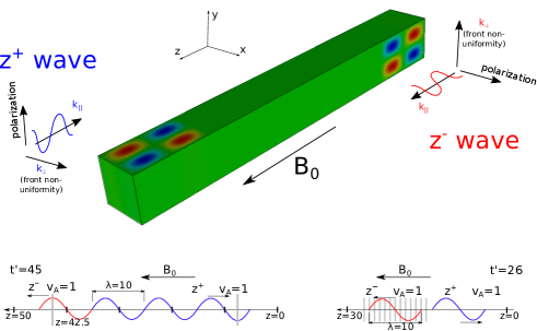
Figure 1: Top: physical setup, early phase. The green rectangle denotes the numerical box with equilibrium plasma, the red and blue areas represent velocity perturbations (positive and negative) of the $z^{-}$ wave (far boundary) and $z^{+}$ wave (near boundary). Polarization planes and non-uniformity directions are annotated. Bottom: longitudinal sketches, late phase after AWs collision: main setups with 1 period in $z^{-}$ and 3 periods in $z^{+}$ wave (left), and complimentary setups with 1 periods in both waves (right). The grey areas denote cross-sections taken for further analysis.

Table 1: Parameters of the numerical setups.

Main setups:
High-resolution
Numerical box	$256\times 256\times 512$ pixels
$L_{z}$	50 Mm
$L_{x}$, $L_{y}$	equal to $\lambda_{\perp}$
Number of periods	$z^{-}$ – 1 period
	$z^{+}$ – 3 periods
$u$	0.1 (same for $z^{-}$ and $z^{+}$)
$\lambda_{z}$ (or $\lambda_{\parallel}$)	10 Mm
$\lambda_{\perp}$	from 0.4 to 25.0 (10 configurations)
$k_{\perp}$	from 15.7 to 0.25
$k_{\perp}/k_{\parallel}$	from 25.0 to 0.4
Low-resolution
Numerical box	$128\times 128\times 256$ pixels
$L_{z}$	50 Mm
$L_{x}$, $L_{y}$	equal to $\lambda_{\perp}$
$u$	0.033 (same for $z^{-}$ and $z^{+}$)
$\lambda_{z}$ (or $\lambda_{\parallel}$)	10 Mm
$\lambda_{\perp}$	from 0.16 to 25.0 (12 configurations)
$k_{\perp}$	from 39.3 to 0.25
$k_{\perp}/k_{\parallel}$	from 62.5 to 0.4
Non-zero cross-helicity:
Numerical box	$256\times 256\times 364$ pixels
$L_{z}$	30 Mm
$L_{x}$, $L_{y}$	equal to $\lambda_{\perp}$
Number of periods	$z^{-}$, $z^{+}$ – 1 period
$u^{-}$	0.1
$u^{+}$	0.03
$\lambda_{z}$ (or $\lambda_{\parallel}$)	10 Mm
$\lambda_{\perp}$, $k_{\perp}$, $k_{\perp}/k_{\parallel}$	same as in high-resolution main setups
Perpendicular and longitudinal structure:
Numerical grid	$256\times 256\times 364$ pixels
$L_{z}$	30 Mm
$L_{x}$, $L_{y}$	equal to $\lambda_{\perp}$
Number of periods	$z^{-}$, $z^{+}$ – 1 period
$u$	0.1 (same for $z^{-}$ and $z^{+}$)
$\lambda_{z}$ (or $\lambda_{\parallel}$)	10 Mm
$\lambda_{\perp}$, $k_{\perp}$, $k_{\perp}/k_{\parallel}$	same as in high-resolution main setups

The numerical box has physical $z$-length $L_{z}$ either 50 Mm (main setups) or 30 Mm (complementary setups). The sizes along $x$ and $y$ are set equal to the perpendicular wavelength $\lambda_{\perp}$ (hence change from setup to setup). The numerical box for the main setups has either $256\times 256\times 512$ pixels (high-resolution) or $128\times 128\times 256$ pixels (low-resolution). We have verified that the decrease of numerical resolution does affect the results: the waves start to decay during their propagation and the wave profiles get distorted. However, this effect is small even for the case of low-resolution setups. In complimentary setups the numerical box always has $256\times 256\times 384$ pixels, thus its spatial resolution coincides with that of the high-resolution setups. We compared various numerical schemes and parameters of MPI-AMRVAC and chose the best settings (powel scheme for the $\mathbf{\nabla\cdot B}$ corrector, high-resolution numerical box etc.). We also pay special attention to distinguish the physical phenomena from numerical artifacts.

3 Results

3.1 Nonlinear effects in a single AW

First we verify the effect of nonlinear self-interaction within a single Alfvén wave. In Fig. 2 we show the longitudinal (along $z$) profiles of $v_{x}$, $v_{y}$, and $v_{z}$ of the forward Alfvén wave, initiated via boundary conditions described in Sect. 2, during its developed phase, but before the collision with the backward wave. For visualization the quantities are normalized by the following constants: the mother wave $v_{x}$ by the initial amplitude $u=0.10$, the horizontal component $v_{y}$ and the ponderomotive component $v_{z}$ by $A_{p}=2.53\cdot 10^{-3}$.

The amplitude and spatial structure of the ponderomotive component $v_{z}$ perfectly reproduces theoretical predictions: its wavenumbers are two times larger than in the mother wave and its amplitude varies from 0 to 2 (McLaughlin et al., 2011; Zheng et al., 2016). We also observed a self-consistent generation of $v_{y}$ that appears only in oblique waves with $\lambda_{\perp}\neq 0$ ($v_{y}=0$ at $\lambda_{\perp}=0$). Our preliminary simulations (two-dimensional setups were sufficient there) have shown the following trend in the variation of $v_{y}$ with varying cross-field wavelength: the amplitude of $v_{y}$ grows proportionally to $1/\lambda_{\perp}$ at the larger scales $\lambda_{\perp}>\lambda_{z}$, this growth slows down at $\lambda_{\perp}\sim\lambda_{z}$, and eventually $v_{y}$ becomes a constant independ on $\lambda_{\perp}$ at smaller scales $\lambda_{\perp}\ll\lambda_{z}$. The spatial extension of $v_{y}$ in both parallel and perpendicular directions is two times shorter than of the mother wave. The amplitude of $v_{y}$ is always smaller than that of $v_{z}$. Similar perturbations of perpendicular velocity were observed also in torsional waves (Shestov et al., 2017).

The observed perturbations of $v_{y}$ and $v_{z}$ propagate along the magnetic field with the Alfvén speed $v_{A}$ and are natural companions of AWs not caused by the numerical effects or boundary conditions for $v_{z}$. The perturbations always develop in AWs regardless of the ways how the waves are initiated – by boundary or initial conditions, with or without boundary perturbations given by Eqs. 7 and 10. In other words, the observed propagating wave is the eigenmode of the compressible nonlinear MHD.

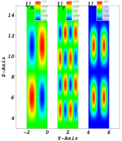
Figure 2: Velocities $v_{x}$ (left), $v_{y}$ (middle), and $v_{z}$ (right) in a single Alfvén wave. The color tables (inlines in top) have different amplitudes in different panels to reflect the range of velocities

. Initially in the Alfvén wave only $v_{x}$ and $B_{x}$ (not shown) and $v_{z}$ are driven; the $v_{y}$ component of the velocity is generated self-consistently due to nonlinear self-interaction within the Alfvén wave.

We thus observe typical characteristics of AWs before they collide.

3.2 AWs collision

To study effects of the AW collisions, we let the two counter-propagating waves to fully propagate through each other, and analyze perpendicular profiles of $v_{x}$ of the forward-propagating $z^{-}$ wave in its leading maximum – $x-y$ plane with $z=42.5$ at instant $t=45$, see Fig. 1, bottom left panel (main setups with $u=0.1$ are used). In Fig. 3 the panels show $v_{x}$ of three different setups with $\lambda_{\perp}=0.5$, $0.8$, and $3.0$ Mm. The perturbations of the wave profiles depend on the perpendicular scale: they are significant for smallest $\lambda_{\perp}=0.5$, moderate for $\lambda_{\perp}=0.8$, and weak for the largest $\lambda_{\perp}=3.0$. Similar perturbations are also observed in the $z^{+}$ wave. However, in setups with only one wave present, such perturbations do not appear, and hence their development can be attributed to AWs collision.

Figure 3: Comparison of perpendicular profiles of $v_{x}$ in the leading maximum of the $z^{-}$ wave in setups with $\lambda_{\perp}=0.5$ (left), $0.8$ (middle), and $3.0$ Mm (right). The axes are in Mm and are different in every panel.

Appearance of such small-scale perturbations propagating with Alfvén velocity can be treated as generation of new AWs at smaller perpendicular scales $\lambda_{\perp}^{\prime}<\lambda_{\perp}$.

3.3 Dependence on perpendicular scales

In order to distinguish the nonlinearly generated waves from the mother wave, we further analyze the wave profiles in the perpendicular cross-section of $z^{-}$ wave. We extract the perturbed velocity $\Delta v_{x}$ by subtracting the initial harmonic profile of $v_{x}$, $\Delta v_{x}=v_{x}-A\sin(k_{\perp}^{-}y)$, where the amplitude $A$ is adjusted to cancel the perturbation in the wave maximum. The results are shown in Fig. 4 for the setups with $\lambda_{\perp}=0.8$ (top panels) and $\lambda_{\perp}=3.0$ (bottom panels). The left panels show $v_{x}$, middle $\Delta v_{x}$, and right $v_{y}$. The induced velocities $\Delta v_{x}$ and $v_{y}$ have amplitudes $\sim(0.02\div 0.03)u$ and are non-uniform in both $x$ and $y$ directions.

To evaluate numerical effects, we made the similar analysis for $z^{-}$ wave in the absence of $z^{+}$ waves. Here the perturbations $\Delta v_{x}$ are observed as well; but they have at least factor 10 smaller amplitude and are uniform along $x$. It means that numerical effects produce significantly weaker perturbations with different spatial profiles. On the contrary, after collisions with counter-propagating $z^{+}$ waves, the perturbations co-propagating with $z^{-}$ waves have both $v_{x}$ and $v_{y}$ components, larger amplitudes, and profiles non-uniform both along $y$ and $x$, which cannot be ascribed to numerical effects. Furthermore, the perturbations of $v_{y}$ generated by the AW collisions can not be attributed solely to the single AW self-interaction where perturbations of the $v_{y}$ are zero at the original wave maximum.

The spatial patterns of the induced velocities fall in two distinct groups: all spatial patterns at $\lambda_{\perp}<\lambda_{\perp}^{tr}$ are similar to that shown on the top panels in Fig. 4, and all patterns at $\lambda_{\perp}\geq\lambda_{\perp}^{tr}$ are similar to that shown on the bottom panels (the transition scale $\lambda_{\perp}^{tr}=3.0$ for $u=0.1$ used in this figure). The perturbations in the former group have a current-sheet structuring, similar to that reported by Verniero et al. (2018) for the strong turbulence regime. The perturbations in the second group have symmetric structure. The same two groups of spatial structures are also observed in the setups with different amplitudes $u$, but with different transition scales, such that $\lambda_{\perp}^{tr}$ is larger for smaller $u$ (for example, $\lambda_{\perp}^{tr}=4.0$ for $u=0.033$).

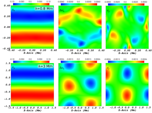
Figure 4: Perpendicular profiles of velocities in setups with $\lambda_{\perp}=0.8$ (top) and $\lambda_{\perp}=3$ (bottom). Left: measured $v_{x}$; middle: difference $\Delta v_{x}$ between the measured $v_{x}$ and a harmonic function; right: measured $v_{y}$. Perturbations of $\Delta v_{x}$ and $v_{y}$ are produced in result of AWs collision. In each panel the color table matches the maximum amplitude of the measured quantity.

The dependence of the amplitudes of induced waves on the perpendicular scales is shown in Fig. 5. The diamonds correspond to $\Delta v_{x}$ and asterisks correspond to $v_{y}$. For $u=0.1$ the symbols are blue and green, for $u=0.033$ they are orange and red. Gray and pink regions indicate the wavenumber ranges where the wave collisions should generate the strong (critically balanced) turbulence with $k_{\perp}/k_{\parallel}\sim v_{A}/u$ for $u=0.1$ and $u=0.033$, respectively. In both these cases the amplitude behavior is similar. At largest $\lambda_{\perp}$ the amplitudes of the induced waves are much smaller than the amplitudes of the original waves and the resulting AW turbulence should be weak. As $\lambda_{\perp}$ decreases, the induced amplitudes first increase slowly and reach a maximum. This maximum is still much smaller than the initial AW amplitude and is reached at $\lambda_{\perp}=\lambda_{\perp\mathrm{max}}$ that is still much larger than the perpendicular scale given by the critically balance condition, $\lambda_{\perp\mathrm{max}}\gg$ $\lambda_{\perp\ast}=\lambda_{\parallel}u/v_{A}$ ($\lambda_{\perp\mathrm{max}}$, $\lambda_{\perp\ast}$ and other characteristic perpendicular scales are shown in Fig. 5). When $\lambda_{\perp}$ decreases further beyond $\lambda_{\perp\mathrm{max}}$, the induced amplitudes decrease and reach a minimum at $\lambda_{\perp}=$ $\lambda_{\perp\mathrm{min}}$ that is still larger than $\lambda_{\perp\ast}$. After this minimum, a strong increase of induced perturbations occurs in the region where $\lambda_{\perp}$ becomes several times shorter than $\lambda_{\perp\ast}$. Amplitudes of generated perturbations become there comparable to the amplitudes of initial waves and such collisions can generate strong turbulence.

While the observed strengthening of the nonlinear interaction with decreasing $\lambda_{\perp}$ is expected taking into account that the responsible nonlinear term is $\sim\left(\mathbf{z}\cdot\nabla\right)\mathbf{z\sim}$ $\lambda_{\perp}^{-1}$, the depression observed at $\lambda_{\perp}\gtrsim$ $\lambda_{\perp\ast}$ and its influence on the transition from weak to strong turbulence need further investigations. At present we can only state that this depression should result in a shift of the weak-strong turbulence transition to the perpendicular scales significantly shorter than that prescribed by the standard critical balance condition.

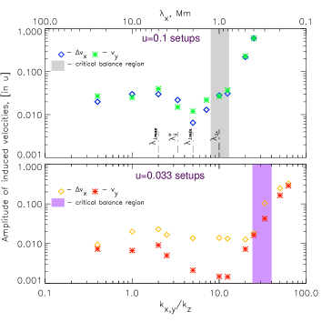
Figure 5: Dependence of the amplitudes of the induced waves on $k_{\perp}/k_{\parallel}$ of the original wave for the $u=0.1$ (top) and $u=0.033$ (bottom) setups. Diamonds and asterisks correspond to the $\Delta v_{x}$ and $v_{y}$ respectively. Filled areas correspond to the regions of classic critical balance in incompressible MHD calculated for particular $u$. In the top panel the values of $\lambda_{\perp\mathrm{max}}$, $\lambda_{\perp\mathrm{min}}$, $\lambda_{\perp}^{tr}$, and $\lambda_{\perp*}$ are shown.

3.4 Influence of several collisions

Since the initiated $z^{-}$ and $z^{+}$ waves contain 1 and 3 periods, respectively, the $z^{-}$ wave can interact with 3 periods of the counter-propagating wave, whereas each period of the $z^{+}$ wave can interact with only one period of $z^{-}$. We thus expect different amplitudes of the induced perturbation propagating in $z^{-}$ and $z^{+}$ directions. To verify this, we measure the perturbations accompanying the $z^{+}$ wave using the same technique as for $z^{-}$ wave (remember that in $z^{+}$ wave the roles of $v_{x}$ and $v_{y}$ are exchanged). Comparison of the corresponding perturbations in the $z^{-}$ and $z^{+}$ waves is given in Fig. 6. The top panel shows the amplitudes of perturbations accompanying $z^{-}$ (blue and green symbols) and $z^{+}$ (orange and red symbols), the bottom panel shows the ratio $z^{-}/z^{+}$ of the perturbations with the corresponding (orthogonal) polarizations. In both panels the diamonds denote perturbations with the same polarization as in the original waves ($\Delta v_{x}$ in $z^{-}$, $\Delta v_{y}$ in $z^{+}$), and the asterisks denote the complimentary polarization.

The behavior of $z^{+}$ perturbations as function of $\lambda_{\perp}$ is qualitatively similar to that of $z^{-}$ perturbations. At smallest $\lambda_{\perp}$ the ratio of the $-/+$ perturbations is about 2, then approaches 3 with the scale increase, then increases significantly at $\lambda_{\perp}/\lambda_{\parallel}\sim 1$, and finally drops again to 2 at large perpendicular scales $\lambda_{\perp}/\lambda_{\parallel}>1$. In the region of (super-)strong turbulence the observed ratio $z^{-}/z^{+}<3$ means inapplicability of the perturbation theory: already after the first interaction the wave profiles are distorted significantly and the following collisions do not add much.

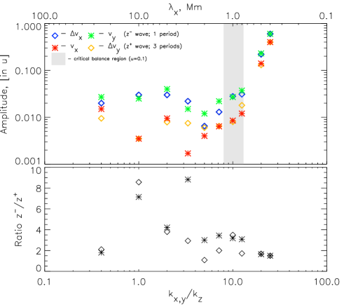
Figure 6: Dependence of the amplitudes of induced waves on the wavenumber ratio for different number of wave collisions ($z^{-}$ wave collides 3 times and $z^{+}$ wave collides once). Top: amplitudes of the perturbations. Bottom: ratio of the amplitudes $z^{-}/z^{+}$, diamonds correspond to original polarization ($v_{x}$ in $z^{-}$, and $v_{y}$ in $z^{+}$) and asterisks correspond to perpendicular polarization.

3.5 Non-zero cross-helicity case

In this section we analyze the effects of non-zero cross-helicity (imbalance) when the counter-propagating initial waves have different amplitudes. This situation is common in the fast solar wind (Tu et al., 1990; Lucek & Balogh, 1998) and also occurs in numerical simulations in local subdomains of the simulation box (Perez & Boldyrev, 2009).

We run dedicated setups with initial amplitudes $u^{-}=0.1$ in $z^{-}$ wave and $u^{+}=0.033$ in $z^{+}$ wave, both waves have one period. We compare measured perturbations with our main setups in Fig. 7. The black symbols denote $z^{-}$ perturbation and orange and red symbols denote $z^{+}$ perturbations in imbalanced setups, and blue and green symbols denote main setups ($u=0.1$, 1 period in $z^{-}$ wave and 3 periods in $z^{+}$ wave).

The perturbations observed in imbalanced cases are smaller then in the main setups. At the same time the perturbations (expressed in initial amplitudes $u$) in the $z^{-}$ wave are $\sim 3$ times smaller then in the $z^{+}$ wave.

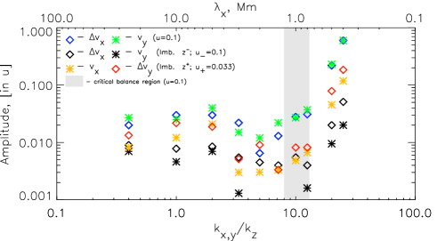
Figure 7: Amplitude of the induced waves for the case of non-zero cross-helicity: $u^{-}=0.1$, $u^{+}=0.033$, each wave has single period. Black symbols denote perturbations in the $z^{-}$ wave, orange and red symbols denote perturbations in the $z^{+}$ wave. Blue and green symbols represent the main setups ($u=0.1$, 1 and 3 periods respectively).

3.6 Perpendicular Fourier spectra

In order to understand the spectral transport generated by the AW collisions, we analyze the spatial Fourier spectra of the induced waves. The spectra of the $v_{x}$ and $v_{y}$ velocities at the leading maximum of $z^{-}$ are given in Fig. 8 for $\lambda_{\perp}=0.8$ in the top row, $\lambda_{\perp}=2.0$ in the middle row, and $\lambda_{\perp}=3.0$ in the bottom row. On the left panels, the spectra of $v_{x}$ in a single $z^{-}$ wave are shown, on the middle and right panels the spectra of $v_{x}$ and $v_{y}$ after the AW collision are shown. In each panel the $(x,y)$-coordinates represent corresponding Fourier wavenumbers and the color shows intensity of a given spectral component. The quasi-logarithmic color scale is normalized to the intensity of an ideal harmonic function $u\sin(k_{\perp}^{-}y)$. This function would have only two peaks with spectral coordinates $(0,\pm 1)$ that correspond to the brightest components in the left and middle panels. In what follows, we will drop the $\pm$ sign keeping in mind the inherent symmetry.

The higher-wavenumber spectral components $(0,\left|y\right|>1)$ accompanying the single $z^{-}$ wave without collisions (left panels) are due to numerical effects. Note the low level of these components and their uniform distribution. On the contrary, the real spectral components with higher wavenumbers are generated by the AW collisions (middle and right panels).

The strongest induced components at $\lambda_{\perp}=0.8$ have spectral coordinates $(1,2)$ corresponding to the perpendicular wavevector $\mathbf{k_{\perp}}=k_{\perp}^{+}\mathbf{\hat{x}}+2k_{\perp}^{-}\mathbf{\hat{y}}$. Generation of waves with such wavevectors supports the mechanism proposed by Howes & Nielson (2013) (see their Fig. 2 explaining appearance of such “tertiary” waves). This mechanism is summarized in the Introduction.

The same Fourier components $(1,2)$ of $v_{x}$ are also seen in the middle row Fig. 8 in the case of intermediate scale $\lambda_{\perp}=2$; in addition, the spectral components of $v_{x}$ with coordinates $(1,1)$ corresponding to $\mathbf{k_{\perp}}=k_{\perp}^{+}\mathbf{\hat{x}}+k_{\perp}^{-}\mathbf{\hat{y}}$ are significant as well.

The spatial spectra of $v_{x}$ and $v_{y}$ at the largest scale $\lambda_{\perp}=3$ are qualitatively different: the strongest induced components have coordinates $(1,1)$ while the others are negligible. These spectral components might be formed by a different mechanism than in the $\lambda_{\perp}=0.8$ case.

In general, the spectral dynamics observed in our simulations, i.e. generation of higher-wavenumber spectral components, supports scenarios with direct turbulent cascades generated by AW collisions.

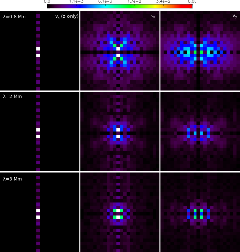
Figure 8: Perpendicular Fourier spectra of $v_{x}$ and $v_{y}$ velocities measured in the leading maximum of the $z^{-}$ wave. Top row: $\lambda_{\perp}=0.8$; middle row: $\lambda_{\perp}=2$; bottom row: $\lambda_{\perp}=3$. Left: $v_{x}$ of the setup with the $z^{-}$ wave only; middle and right denote $v_{x}$ and $v_{y}$ of the setups after AWs collision. In each panel the $(x,y)$-coordinates represent corresponding Fourier wavenumbers and the color shows intensity of a given spectral component. The quasi-logarithmic color table is normalized to the amplitude of a harmonic wave.

3.7 Field-aligned structure of the induced Alfvén waves

Longitudinal behavior of the Fourier components of the induced Alfvén waves is studied using the following approach: we Fourier-analyze perpendicular cross-sections at multiple $z$-coordinates, covering the distance of slightly more then one full wavelength $\lambda_{\parallel}$ along $z$ (see bottom right sketch in Fig. 1). In Fig. 9 we show longitudinal behaviour of the spectral components of $v_{x}$ with coordinates $(0,1)$, $(1,1)$, $(1,2)$, $(2,1)$, and $(2,2)$ with different colors. The mother wave with spectral coordinates $(0,1)$ is shown with black. The top panel shows the setups with $\lambda_{\perp}=0.5$, and the bottom panel shows the setup with $\lambda_{\perp}=2.0$. The intensity of the spectral components is multiplied by factor 10 in the top panel, and by factor 100 in the bottom panel.

We observe drastically different behavior of the spectral components in different setups. While we do not see any regularity in the larger-scale setup, in the setup with $\lambda_{\perp}=0.5$ the growth of $(1,1)$ and $(1,2)$ components is highly correlated and their parallel scales are somehow shorter than in initial AWs. In addition, the energy of the induced waves tend to concentrate near the center of the mother wave.

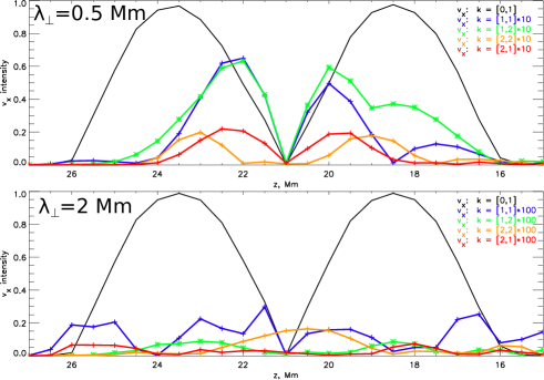
Figure 9: Longitudinal dependence of amplitudes of spatial Fourier components of $v_{x}$. Top: setup with $\lambda_{\perp}=0.5$; bottom: setup with $\lambda_{\perp}=2$ Mm. Different colors correspond to particular spectral coordinates.

4 Discussion and Application

Results of our simulations revealed several new properties of AW collisions in compressional plasmas, which can affect Alfvénic turbulence and anisotropic energy deposition in plasma species. The most striking new property is the modified relation between the parallel and perpendicular scales in the strong turbulence regime where the energy is efficiently transferred to the smaller scale during one collision.

The turbulence strength is usually characterized by the nonlinearity parameter $\chi_{k}\equiv\tau_{k}^{\mathrm{L}}/\tau_{k}^{\mathrm{NL}}=\left(k_{\perp}v_{k}\right)/\left(k_{z}v_{A}\right)$, where $\tau_{k}^{\mathrm{NL}}=\lambda_{\perp}/v_{k}=2\pi/\left(k_{\perp}v_{k}\right)$ is the nonlinear mixing time, $\tau_{k}^{\mathrm{L}}=\lambda_{z}/v_{A}=2\pi/\left(k_{z}v_{A}\right)$ is the linear (correlation) crossing time of colliding AWs, and $v_{k}$ is the velocity amplitude of the colliding AWs. Denote by $\delta v_{k}$ the velocity amplitude of generated waves. When the classic critical balance condition of incompressible MHD is satisfied,

$$\chi_{k}=1,$$ (11)

the nonlinear mixing becomes as fast as the linear crossing and the turbulence is believed to be strong, $\delta v_{k}/v_{k}\sim 1$ (Goldreich & Sridhar, 1995).

However, as follows from our simulations (see e.g. Fig. 5 showing $\delta v_{k}/v_{k}$ as function of $k_{\perp}/k_{z}$ for two fixed amplitudes, $u\equiv v_{k}/v_{A}=0.1$ and $0.033$, and $\delta v_{k}=\sqrt{\Delta v_{x}^{2}+v_{y}^{2}}$), the spectral transport in compressible MHD is strongly, about one order of magnitude, suppressed at $k_{\perp}/k_{z}$ satisfying Eq. 11. Namely, $\delta v_{k}/v_{k}\ll 1$ at $k_{\perp}/k_{z}=10$ for $u=0.1$ and at $k_{\perp}/k_{z}=30$ for $u=0.033$. At $k_{\perp}/k_{z}$ increasing further, the spectral transport eventually becomes fast and the turbulence strong, $\delta v_{k}/v_{k}\sim 1$, which happens at $k_{\perp}/k_{z}$ obeying the modified critical balance condition

$$\tilde{\chi}_{k}=\alpha\chi_{k}=1,$$ (12)

where $\alpha<1$ is the factor reducing efficiency of the nonlinear mixing (in other words, the effective nonlinear time increases by the factor $1/\alpha$). Consequently, the turbulence becomes strong at perpendicular wavenumbers that are larger than in the classic critically balanced case.

The origin and nature of $\alpha$ need further clarification. Since $\alpha\neq 1$ arises when the plasma compressibility is taken into account, it should depend on the relative content of thermal energy, e.g. on the plasma $\beta$. For parameters adopted in our simulations, $\alpha\approx 0.3$ in the critically-balanced state where the scale ratio $k_{\perp}/k_{z}$ obeys $\tilde{\chi}_{k}\sim 1$. Such departure from the classic critical balance affects dynamics of the strong AW turbulence (see below). In the general case of arbitrary scales the functional dependence $\alpha=\alpha\left(\beta,v_{k},k_{\perp}/k_{z}\right)$ is complex; in particular, $\delta v_{k}/v_{k}$ becomes a decreasing function of $k_{\perp}/k_{z}$ in some interval (in Fig. 5 it happens at $k_{\perp}/k_{z}\lesssim 10$), which should greatly affect the weak AW turbulence. We do not exclude that $\alpha$ may also depend on other plasma/wave parameters.

Let us consider the Alfvénic turbulence driven by the fluctuating velocity $v_{k0}$ at the wavenumber ratio $k_{\perp 0}/k_{z0}$ obeying the critical balance condition $\tilde{\chi}_{k0}=1$, in which case the turbulence is already strong at the driving scales. The spectral energy flux in the inertial range is

$$\epsilon_{s}=\frac{\rho v_{k}^{2}}{\tau_{k}^{\mathrm{L}}}=\alpha\frac{\rho v_{k}^{2}}{\tau_{k}^{\mathrm{NL}}}\approx\alpha\frac{\rho v_{k}^{3}k_{\perp}}{2\pi}=\mathrm{const}\equiv\alpha_{0}\frac{\rho v_{k0}^{3}k_{\perp 0}}{2\pi},$$ (13)

where $\tau_{k}^{\mathrm{L}}=\lambda_{z}/v_{A}$ is the AW collision time and $\rho\approx n_{0}m_{i}$ is the mass density. Note that the spectral flux $\epsilon_{s}$ from Eq. 13 is reduced as compared to the incompressible strong turbulence driven at the same perpendicular scale, but remains the same for the turbulence driven at the same parallel scale.

Assume that there is a weak dependence $\alpha=\alpha_{0}\left(v_{k}/v_{k0}\right)^{\delta}$, where $0<\delta<3/4$. Such dependence is suggested by the following semi-empirical considerations. As the observed spectra are power-law, the scaling of $\alpha$ with $v_{k}$ should be power law as well. Furthermore, the index $\delta$ of the power-law dependence should be small positive to reproduce the observed in simulations mismatch between the classic and real critical balances (which is larger for larger wave amplitude). Moreover, such positive values of $\delta$ appear to be compatible with the observed spectral indexes of turbulence in the quasi-stationary solar wind, which are slightly larger than $-5/3$ (up to $-3/2$).

The kinetic energy spectrum is then flatter than the Kolmogorov one,

$$W_{s\perp}\sim v_{k}^{2}/k_{\perp}\sim k_{\perp}^{-5/3+2\delta/9},$$ (14)

and its spectral index varies between $-5/3$ and $-3/2$, as is typically observed in the solar wind turbulence. In the case of $\alpha$ constant along the critical balance path, $\delta=0$, the spectrum reduces to the classic Kolmogorov $W_{s\perp}\sim v_{k}^{2}/k_{\perp}\sim k_{\perp}^{-5/3}.$ The parallel wavenumber spectrum is, as usual, $W_{sz}\sim v_{k}^{2}/k_{z}\sim k_{z}^{-2}$.

If the turbulence is weak at injection, $\tilde{\chi}_{k0}=\delta v_{k0}/v_{k0}<1$, the cascade time increases from the strong turbulence value $\tau_{k}^{\mathrm{TC}}\sim\tau_{k}^{\mathrm{L}}$ to the weak turbulence value $\tau_{k}^{\mathrm{TC}}\sim\left(\delta v_{k}/v_{k}\right)^{2}\tau_{k}^{\mathrm{L}}$. The resulting weakly turbulent energy flux $\epsilon_{w}$ decreases as compared to the strongly turbulent energy flux (13), $\epsilon_{w}=\tilde{\chi}_{k}\epsilon_{s}$:

$$\epsilon_{w}=\frac{\rho v_{k}^{2}}{\tau_{k}^{\mathrm{TC}}}=\frac{\rho v_{k}^{2}}{\tau_{k}^{\mathrm{L}}}\tilde{\chi}_{k}^{-2}=\mathrm{const}\equiv\frac{\rho v_{k0}^{2}}{\tau_{k0}^{\mathrm{L}}}\tilde{\chi}_{k0}^{-2}.$$ (15)

The weakly turbulent spectrum is problematic to calculate because of a complex dependence of $\delta v_{k}/v_{k}$ upon $k_{\perp}$ and $v_{k}$ (see Fig. 5), which is unknown and difficult to guess. At present, we can only note that the strength $\tilde{\chi}_{k0}$ of the compressional weak turbulence is much (about one order, as is demonstrated by Fig. 5) smaller than the incompressional one, $\tilde{\chi}_{k0}\ll\chi_{k0}$, which drastically decreases the weakly turbulent energy flux.

Although the large-scale MHD AWs do not dissipate directly, the turbulent cascade transfers their energy to small scales where dissipative effects come into play heating plasma. MHD Alfvénic turbulence has been employed as the mechanism for plasma heating in the solar corona and solar wind, both from the theoretical/modeling perspective (Van Ballegooijen et al., 2011; Verdini, A. et al., 2012) and based on experimental observations of quiescent (Morton et al., 2016; De Moortel et al., 2014; Xie et al., 2017) and flaring loops (Doschek et al., 2014; Kontar et al., 2017). Here we discuss how the new properties of AW collisions observed in our simulations can affect models of quasi-steady turbulent plasma heating in coronal loops.

Recently, Xie et al. (2017) analyzed as many as 50 loops in active regions using observations of Extreme-ultraviolet Imaging Spectrometer (EIS) (Culhane et al., 2007) on board the Hinode satellite. They observed non-thermal widths of spectral lines and found corresponding non-thermal velocities in the range $v_{\mathrm{nt}}=30\div 40$ km s^-1, magnetic field in the loop apexes up to 30 G, loop widths $L_{\perp}\sim 2\div 4$ Mm and loop lengths $L_{z}\sim 100$ Mm. Brooks & Warren (2016) also used spectroscopic data from EIS and evaluated non-thermal velocities in loops in 15 active regions. The typical values were somewhat smaller, with typical values $v_{\mathrm{nt}}\sim 20$ km s^-1; the authors however did not provide any other parameters. Furthermore, Gupta et al. (2019) analyzed non-thermal widths of spectral lines in high coronal loops (with heights up to $1.4R_{\odot}$) measured by EIS and found the non-thermal velocities in the range $20\div 30$ km s^-1. The above values can be used to evaluate the turbulent heating of coronal loops.

We assume that there are AW sources at the loop footpoints. These source can be due to magnetic reconnection and/or photospheric motion (we will not specify their origin in more details here). The perpendicular AW wavelengths $\lambda_{\perp 0}$ are limited by the cross-$\mathbf{B}_{0}$ scale $l_{\perp}$ of density filaments comprising the loops, $\lambda_{\perp 0}\lesssim l_{\perp}$ (wavenumber $k_{\perp 0}\gtrsim 2\pi/l_{\perp}$). Note that $l_{\perp}$ can be significantly smaller than the visible loop width $r$. On the contrary, the coronal plasma is quite homogeneous along $\mathbf{B}_{0}$ and the possible parallel wavelength $\lambda_{z0}$ are restricted by the loop length $L_{z}$, $\lambda_{z0}=2\pi/k_{z0}\leq L_{z}$ (wavenumber $k_{z0}\gtrsim 2\pi/L$).

For the wavelengths within the mentioned above limits, a large spectral flux, and hence a strong plasma heating, can be established by the strong turbulence driven at the critically-balanced anisotropy $\alpha k_{\perp 0}/k_{z0}=$ $\alpha\lambda_{z0}/\lambda_{\perp 0}=$ $v_{A}/v_{k0}$. The corresponding energy flux injected in the unit volume is $\epsilon_{cor}\approx\alpha_{0}\rho v_{k0}^{3}/\lambda_{\perp 0}$. Assuming that the turbulent velocity at injection $v_{k0}$ is observed as the nonthermal velocity, $v_{k0}\approx v_{\mathrm{nt}}$, and taking from Xie et al. (2017) $v_{\mathrm{nt}}=30$ km s^-1, magnetic field $B=30$ G, and density $n_{e}=2\times 10^{9}$ cm^-3, we obtain the energy flux $\epsilon_{cor}\sim\alpha_{0}\rho v_{\mathrm{nt}}^{3}/l_{\perp}\sim$ $3\times 10^{-4}\left(l_{\perp}/L_{\perp}\right)^{-1}$ erg cm^-3 s^-1. For sufficiently small $l_{\perp}\lesssim 0.1L_{\perp}$, the energy flux $\epsilon_{cor}\gtrsim$ $3\times 10^{-3}$ erg cm^-3 s^-1 is enough to heat typical coronal loops. The corresponding parallel wavelengths at injection are $\lambda_{z0}\sim\left(\alpha v_{\mathrm{nt}}/v_{A}\right)^{-1}\lambda_{\perp 0}\lesssim 0.5L_{z}$. Therefore, the turbulent cascade and related plasma heating can be effective if the perpendicular length scales of the loop substructures are about 10 times smaller than the loop width, which implies that the loops should be structured more than was required by previous turbulent heating models.

5 Conclusions

In the framework of compressional MHD, we studied numerically the spectral transport produced by the collisions between counter-propagating Alfvén waves. The initial two waves are linearly polarized in two orthogonal planes and their cross-field profiles vary normally to their polarization planes. Polarization and spectral characteristics of the perturbations generated after single and multiple collisions between such AWs are analyzed in detail. The main properties of the resulting spectral transfer are as follows:

• the perturbations generated by AW collisions have smaller scales than the original waves, which supports turbulence scenarios based on the direct turbulent cascade generated by AW collisions;

• we observed two regimes of the AW interaction: the first one is typical for the case of strong turbulence, and the second one is governed by a different mechanism;

• the spectral transfer generated by the AW collisions is strongly suppressed at the scales satisfying the classic critical balance condition (11) of incompressional MHD, which makes the turbulence weak at these scales;

• the strong turbulence is re-established at significantly smaller perpendicular scales satisfying the modified critical balance condition (12);

We used these properties to re-evaluate the turbulent heating of the solar coronal loops. The main conclusion is that the turbulent cascade can heat the loop plasma provided the loop is structured and the characteristic widths of the loop sub-structures are more than 10 times smaller than the loop width.

References

- Belcher & Davis (1971) Belcher, J. W. & Davis, L. 1971, Journal of Geophysical Research, 76, 3534
- Beresnyak (2014) Beresnyak, A. 2014, The Astrophysical Journal, 784, L20
- Beresnyak (2015) Beresnyak, A. 2015, The Astrophysical Journal, 801, L9
- Beresnyak & Lazarian (2008) Beresnyak, A. & Lazarian, A. 2008, ApJ, 682, 1070
- Brooks & Warren (2016) Brooks, D. H. & Warren, H. P. 2016, The Astrophysical Journal, 820, 63
- Bruno & Carbone (2013) Bruno, R. & Carbone, V. 2013, Living Reviews in Solar Physics, 10, 2
- Chandran & Perez (2019) Chandran, B. D. G. & Perez, J. C. 2019, Journal of Plasma Physics, 85, 905850409
- Culhane et al. (2007) Culhane, J. L., Harra, L. K., James, A. M., et al. 2007, Sol. Phys., 243, 19
- De Moortel et al. (2014) De Moortel, I., McIntosh, S. W., Threlfall, J., Bethge, C., & Liu, J. 2014, Astrophysical Journal Letters, 782
- Doschek et al. (2014) Doschek, G. A., McKenzie, D. E., & Warren, H. P. 2014, The Astrophysical Journal, 788, 26
- Drake et al. (2016) Drake, D. J., Howes, G. G., Rhudy, J. D., et al. 2016, Physics of Plasmas, 23, 022305
- Drake et al. (2013) Drake, D. J., Schroeder, J. W. R., Howes, G. G., et al. 2013, Physics of Plasmas, 20, 072901
- Drake et al. (2014) Drake, D. J., Schroeder, J. W. R., Shanken, B. C., et al. 2014, IEEE Transactions on Plasma Science, 42, 2534
- Galtier et al. (2000) Galtier, S., Nazarenko, S. V., Newell, A. C., & Pouquet, A. 2000, Journal of Plasma Physics, 63, 447
- Gogoberidze & Voitenko (2016) Gogoberidze, G. & Voitenko, Y. M. 2016, Ap&SS, 361, 364