Phonon renormalization and Pomeranchuk instability in the Holstein model

Abstract

The Holstein model with dispersionless Einstein phonons is one of the simplest models describing electron-phonon interactions in condensed matter. A naive extrapolation of perturbation theory in powers of the relevant dimensionless electron-phonon coupling $\lambda_{0}$ suggests that at zero temperature the model exhibits a Pomeranchuk instability characterized by a divergent uniform compressibility at a critical value of $\lambda_{0}$ of order unity. In this work, we re-examine this problem using modern functional renormalization group (RG) methods. For dimensions $d>3$ we find that the RG flow of the Holstein model indeed exhibits a tricritical fixed point associated with a Pomeranchuk instability. This non-Gaussian fixed point is ultraviolet stable and is closely related to the well-known ultraviolet stable fixed point of $\phi^{3}$-theory above six dimensions. To realize the Pomeranchuk critical point in the Holstein model at fixed density both the electron-phonon coupling $\lambda_{0}$ and the adiabatic ratio $\omega_{0}/\epsilon_{F}$ have to be fine-tuned to assume critical values of order unity, where $\omega_{0}$ is the phonon frequency and $\epsilon_{F}$ is the Fermi energy. However, for dimensions $d\leq 3$ we find that the RG flow of the Holstein model does not have any critical fixed points. This rules out a quantum critical point associated with a Pomeranchuk instability in $d\leq 3$.

I Introduction

Gaining a microscopic understanding of the effect of electron-phonon interactions on the physical behavior of metals continues to be one of the central topics in condensed matter physics. Although model systems for electron-phonon interactions have been studied for many decades using the established machinery of many-body and kinetic theory [1, 2, 3], the limit of strong electron-phonon interactions remains a challenge to theory. It is therefore not surprising that recently numerical calculations have revealed new phenomena in coupled electron-phonon systems which were not anticipated in the older literature, such as the emergence of nontrivial phases with broken symmetry [4, 5, 6, 7, 8, 9, 10] or the existence of several hydrodynamic regimes with distinct temperature dependence of various physical quantities [11]. Let us also point out that a microscopic description of strongly coupled electron-phonon systems in the so-called semiquantum regime [12, 13, 14] $\epsilon_{F}\ll T\ll\omega_{D}\ll V_{\rm cb}$ is still lacking. Here $\epsilon_{F}$ is the Fermi energy, $T$ is the temperature, $\omega_{D}$ is the Debye energy, and $V_{\rm cb}\propto n^{1/3}e^{2}$ is the characteristic Coulomb energy (where $n$ is the electronic density and $-e$ is the electric charge). For simplicity, we measure temperature and frequencies in units of energy, which amounts to formally setting $k_{B}=\hbar=1$.

Given the fact that our understanding of strongly coupled electron-phonon systems is still incomplete, it is useful to approach this problem using complementary methods. While numerical methods have produced a number of interesting results, especially for the phase diagram of coupled electron-phonon systems in two dimensions [4, 5, 6, 7, 8, 9, 10], a deeper understanding of the nature of phase transitions can be gained using renormalization group (RG) methods. Here we study the Holstein model [15] in arbitrary dimensions $d$ using the functional renormalization group [16, 17, 18, 19, 20, 21]. The Holstein model can be obtained as a special case of the Fröhlich model [22] by assuming a local electron-phonon coupling and dispersionless Einstein phonons with frequency $\omega_{0}$. Moreover, the direct Coulomb interaction between the electrons is neglected. In momentum space the Hamiltonian of the Holstein model is

$${\cal{H}} = \sum_{\bm{k}}\epsilon_{\bm{k}}c^{\dagger}_{\bm{k}}c_{\bm{k}}+\omega_{0}\sum_{\bm{q}}b^{\dagger}_{\bm{q}}b_{\bm{q}}+\frac{\gamma_{0}}{\sqrt{\cal{V}}}\sum_{\bm{k},\bm{q}}c^{\dagger}_{\bm{k}+\bm{q}}c_{\bm{k}}X_{\bm{q}},\hskip 19.91692pt$$ (1)

where the operator $c_{\bm{k}}$ annihilates an electron with momentum $\bm{k}$ and energy $\epsilon_{\bm{k}}$, the operator $b_{\bm{q}}$ annihilates a phonon with momentum $\bm{q}$ and energy $\omega_{0}$, and $X_{\bm{q}}=(b_{\bm{q}}+b^{\dagger}_{-\bm{q}})/\sqrt{2\omega_{0}}$ is the Fourier component of the phonon displacement operator. Here ${\cal{V}}$ is the volume of the system, $\bm{k}$-sums are over the first Brillouin zone, $\bm{q}$-sums have an implicit ultraviolet cutoff of the order of the Debye momentum, and we consider spinless electrons for simplicity. The strength of the electron-phonon coupling is characterized by the dimensionless parameter

$$\lambda_{0}=\nu\gamma_{0}^{2}/\omega_{0}^{2},$$ (2)

where

$$\nu=\frac{1}{\cal{V}}\sum_{\bm{k}}\delta(\epsilon_{F}-\epsilon_{\bm{k}})$$ (3)

is the electronic density of states at the Fermi energy.

According to Migdal’s theorem [1], many-body calculations for the Holstein model simplify in the regime

$$\lambda_{0}\omega_{0}/\epsilon_{F}\ll 1,$$ (4)

because then vertex corrections can be neglected. Note that in the adiabatic limit $\omega_{0}\ll\epsilon_{F}$ the condition (4) is satisfied even for large values of $\lambda_{0}$, corresponding to strong electron-phonon interactions. Recently, this generally accepted scenario has been challenged for the two-dimensional Holstein model where, according to Refs. [7, 8, 9], nonperturbative effects become important when $\lambda_{0}$ is of order order unity. The breakdown of Migdal’s theorem for the two-dimensional Holstein model for $\lambda_{0}={\cal{O}}(1)$ is related to the nonperturbative formation of bipolarons [23, 24] in a certain regime of temperatures. In fact, a hint for the breakdown of perturbation theory in the Holstein model for $\lambda_{0}={\cal{O}}(1)$ can already be obtained by calculating the square of the renormalized phonon frequency to first order in $\lambda_{0}$, which yields [22, 25]

$$\tilde{\omega}_{0}^{2}=\omega_{0}^{2}[1-\lambda_{0}+{\cal{O}}(\lambda_{0}^{2})].$$ (5)

If we boldly neglect the higher-order corrections and extrapolate the first-order term in Eq. (5) to intermediate coupling, then we find that the renormalized phonon frequency vanishes for $\lambda_{0}=1$. But the renormalized phonon frequency of the Holstein model is related to the uniform compressibility $\partial\rho/\partial\mu$ via the Ward identity (see Appendix A)

$$\tilde{\omega}_{0}^{2}=\frac{\omega_{0}^{2}}{1+\frac{\gamma_{0}^{2}}{\omega_{0}^{2}}\frac{\partial\rho}{\partial\mu}},$$ (6)

where $\rho$ is the electronic density and $\mu$ is the chemical potential. The vanishing of $\tilde{\omega}_{0}^{2}$ for $\lambda_{0}\rightarrow 1$ is therefore accompanied by a divergence of the compressibility. At this point the system exhibits a Pomeranchuk instability in the zero angular momentum density channel associated with phase separation [26]. Usually Pomeranchuk instabilities in Fermi systems result from an effective electron-electron interaction [26, 27, 28, 29, 30, 31]. Although the Holstein model does not include a direct interaction between the fermions, by integrating over the phonons we can map the Holstein model onto an effective fermion model with a retarded two-body interaction, see Eq. (84) below. The Pomeranchuk instability in the Holstein model can therefore be interpreted conventionally as an instability of the Fermi liquid triggered by strong electron-electron interactions. We will come back to this interpretation in Sec. III.3, where we also discuss the phase diagram which we show in Fig. 6. Historically, the vanishing of the perturbatively renormalized phonon frequency for strong electron-phonon coupling has already been noticed by Fröhlich [22], but the question whether this is a physical property of the Holstein model, or an artefact of the extrapolation of the first-order result (5) has never been clarified. Although some authors believe that in three dimensions the Holstein model does not exhibit a Pomeranchuk instability [25], we have not been able to find a thorough investigation of this point in the literature.

In this work we re-examine this problem using modern FRG methods [16, 17, 18, 19, 20, 21]. Our main result is that for $d>3$ the RG flow of the Holstein model indeed exhibits tricritical, ultraviolet-stable fixed point which can be associated with a quantum critical point where the system exhibits a Pomeranchuk instability. However, for dimensions $d\leq 3$ the RG flow of the Holstein model does not have any nontrivial fixed points but exhibits a runaway flow, which rules out a Pomeranchuk instability characterized by a divergent uniform compressibility. While the interpretation of the runaway RG flow at some finite scale is not unique, in Sec. III.3 we argue that it indicates either a charge-density wave instability or a first-order transition into an inhomogeneous state characterized by phase separation.

II Pomeranchuk instability from perturbation theory

II.1 Calculation to second order in $\lambda_{0}$

If we ignore the corrections of order $\lambda_{0}^{2}$ in the perturbative expansion (5) of the renormalized phonon frequency, we find that the phonons soften for $\lambda_{0}=1$. This value is of course not reliable and it is possible that the true renormalized phonon frequency $\tilde{\omega}_{0}(\lambda_{0})$ never vanishes, even for large values of $\lambda_{0}$. As a first step in our investigation of this possibility, let us explicitly calculate the correction of order $\lambda_{0}^{2}$ to the renormalized phonon frequency $\tilde{\omega}_{0}^{2}$. Therefore we start from the Euclidean action of the Holstein model (1) and integrate over the momentum conjugate to the phonon displacement $X_{Q}$ to arrive at the action

$$S[\bar{c},c,X] = -\int_{K}{G}_{0}^{-1}(K)\bar{c}_{K}c_{K}+\frac{1}{2}\int_{Q}D_{0}^{-1}(Q)X_{-Q}X_{Q}$$ (7)

$$+\gamma_{0}\int_{K}\int_{Q}\bar{c}_{K+Q}c_{K}X_{Q},$$

where $c_{K}$ and $\bar{c}_{K}$ are Grassmann fields, the real bosonic field $X_{Q}$ represents the phonon displacement, and the inverse noninteracting electron and phonon propagators are given by

$$G_{0}^{-1}(K) = i\omega-\epsilon_{\bm{k}}+\mu,$$ (8)

$$D_{0}^{-1}(Q) = \bar{\omega}^{2}+\omega_{0}^{2}.$$ (9)

For convenience we have introduced collective labels $K=(\bm{k},i\omega)$ and $Q=(\bm{q},i\bar{\omega})$, where $i\omega$ are fermionic Matsubara frequencies and $i\bar{\omega}$ are bosonic ones. The integration symbols are defined by $\int_{K}=\frac{1}{{\beta\cal{V}}}\sum_{\bm{k}}\sum_{\omega}$ and $\int_{Q}=\frac{1}{\beta{\cal{V}}}\sum_{\bm{q}}\sum_{\bar{\omega}}$, where $\beta=1/T$ is the inverse temperature. The inverse propagators of the interacting system are of the form

$$G^{-1}(K) = i\omega-\epsilon_{\bm{k}}+\mu-\Sigma(K),$$ (10)

$$D^{-1}(Q) = \bar{\omega}^{2}+\omega_{0}^{2}+\Delta(Q),$$ (11)

where $\Sigma(K)$ is the electronic self-energy and the phonon self-energy $\Delta(Q)$ can be expressed in terms of the interaction-irreducible polarization $\Pi(Q)$ as [see Eq. (A32) in Appendix A]

$$\Delta(Q)=-\gamma_{0}^{2}\Pi(Q).$$ (12)

The square of the renormalized phonon frequency for vanishing momentum is given by

$$\tilde{\omega}_{0}^{2}=\omega_{0}^{2}-\gamma_{0}^{2}\lim_{\bm{q}\rightarrow 0}\Pi(\bm{q},0).$$ (13)

To evaluate the $\mathcal{O}(\lambda_{0}^{2})$ contribution to the renormalized squared phonon frequency $\tilde{\omega}^{2}_{0}$, we consider the next-to-leading order contributions to the irreducible polarization $\Pi(Q)$ represented by the diagrams (b)–(f) in Fig. 1. We can, analytically, perform all Matsubara sums and reduce the evaluation of the diagrams, at $T=0$, to a two-dimensional integration over the energy variables $\xi$ and $\xi^{\prime}$. Our result for the $\bm{q}$-limit of the polarization is

$$\Pi(0)=\lim_{\bm{q}\rightarrow 0}\Pi(\bm{q},0)=\nu+\frac{\lambda_{0}}{3}\nu$$

$$+\frac{\gamma_{0}^{2}}{2\omega_{0}}\int_{0}^{\infty}d\xi\int_{0}^{\infty}d\xi^{\prime}\Biggl{[}\frac{4\nu(\mu+\xi)\nu(\mu-\xi^{\prime})}{(\xi+\xi^{\prime}+\omega_{0})^{3}}$$

$$+\frac{\nu(\mu+\xi)\nu^{\prime}(\mu-\xi^{\prime})-\nu(\mu-\xi)\nu^{\prime}(\mu+\xi^{\prime})}{(\xi+\xi^{\prime}+\omega_{0})^{2}}\Biggr{]}+{\cal{O}}(\lambda_{0}^{2}),$$

(14)

where $\nu(\epsilon)=\frac{1}{\cal{V}}\sum_{\bm{k}}\delta(\epsilon-\epsilon_{\bm{k}})$ is the energy-dependent density of states and $\nu^{\prime}(\epsilon)=\partial\nu(\epsilon)/\partial\epsilon$. The term $\lambda_{0}\nu/3$ in the first line of Eq. (14) is due to the tadpole self-energy corrections to the propagators in Fig. 1 (b) and (c), the term in the second line is due to the exchange self-energy diagrams (d) and (e), and the last line involving the derivative of the density of states is due to the vertex correction diagram (f). In the adiabatic limit $\omega_{0}\ll\epsilon_{F}$ the latter is a factor of $\omega_{0}/\epsilon_{F}$ smaller than the self-energy contributions, in accordance with Migdal’s theorem. The double-integral in the second line evaluates to $2\nu^{2}/\omega_{0}$ so that for small $\omega_{0}/\epsilon_{F}$ we obtain for the renormalized phonon frequency

$$\tilde{\omega}_{0}^{2}=\omega_{0}^{2}\left[1-\lambda_{0}-\frac{4}{3}\lambda_{0}^{2}+{\cal{O}}(\lambda_{0}^{3},\lambda_{0}^{2}\omega_{0}/\epsilon_{F})\right].$$ (15)

Neglecting the correction terms, we obtain an improved estimate for the critical value $\lambda_{c}$ of the dimensionless electron-phonon coupling where the Pomeranchuk instability occurs,

$$\lambda_{c}=\frac{\sqrt{57}-3}{8}\approx 0.57.$$ (16)

Surprisingly, the second-order correction reduces the critical value of the electron-phonon coupling. However, the critical $\lambda_{c}$ is still of the order of unity so that the higher orders in Eq. (15) cannot be neglected. In fact, we cannot exclude the possibility that higher orders in $\lambda_{0}$ completely remove the Pomeranchuk instability.

Figure 1: Perturbation series for the phonon self-energy $\Delta(Q)$ in the Holstein model. Wavy lines represent the phonon propagator $D_{0}(Q)$, solid arrows represent the electron propagator $G_{0}(K)$, and black dots represent the bare electron-phonon vertex $\gamma_{{0}}\propto\sqrt{\lambda_{0}}$. Diagram (a) represents the leading-order contribution $-\gamma_{0}^{2}\Pi_{0}(Q)$ to the phonon self-energy, diagrams (b) and (c) are generated by the Hartree corrections to the electronic self-energy, the diagrams (d) and (e) are due to the exchange corrections to the electronic self-energy, and diagram (f) represents the leading vertex correction.

II.2 Effective phonon action and quantum critical point

Since in this work we are only interested in the phonons, or rather the phonon self energy $\Delta(Q)$, it is convenient to integrate over the fermions and work with the effective phonon action. Thus, we may formally perform the Gaussian integration over the electron field to obtain the effective phonon action

$$S_{\rm eff}[X]=\frac{1}{2}\int_{Q}D_{0}^{-1}(Q)X_{-Q}X_{Q}-{\rm Tr}\ln\left[1-\gamma_{0}\mathbf{G}_{0}\mathbf{X}\right],$$ (17)

where $\mathbf{G}_{0}$ and $\mathbf{X}$ are infinite matrices in momentum-frequency space with matrix elements

$$[\mathbf{G}_{0}]_{KK^{\prime}} = \delta_{K,K^{\prime}}G_{0}(K),$$ (18)

$${[}\mathbf{X}{]}_{KK^{\prime}} = X_{K-K^{\prime}},$$ (19)

and the trace is normalized as follows,

$$-{\rm Tr}\ln\left[1-\gamma_{0}\mathbf{G}_{0}\mathbf{X}\right]=-\int_{K}\ln\left[1-\gamma_{0}\mathbf{G}_{0}\mathbf{X}\right]_{KK}$$

$$= \gamma_{0}\int_{K}[\mathbf{G}_{0}\mathbf{X}]_{KK}+\frac{\gamma_{0}^{2}}{2}\int_{K}[\mathbf{G}_{0}\mathbf{X}\mathbf{G}_{0}\mathbf{X}]_{KK}+\ldots$$

$$= \gamma_{0}X_{0}\int_{K}G_{0}(K)$$

$$+\frac{\gamma_{0}^{2}}{2}\int_{K}\int_{K^{\prime}}G_{0}(K)X_{K-K^{\prime}}G_{0}(K^{\prime})X_{K^{\prime}-K}+\ldots\;.$$

The expansion of the effective action $S_{\rm eff}[X]$ in powers of the phonon field is therefore of the form

$$S_{\rm eff}[X]=\Gamma_{0}^{(1)}X_{Q=0}+\frac{1}{2}\int_{Q}\Gamma_{0}^{(2)}(Q)X_{-Q}X_{Q}$$

$$+\sum_{n=3}^{\infty}\frac{1}{n!}\int_{Q_{1}}\cdots\int_{Q_{n}}\delta(Q_{1}+\ldots+Q_{n})$$

$$\hskip 28.45274pt\times\Gamma_{0}^{(n)}(Q_{1},\ldots,Q_{n})X_{Q_{1}}\cdots X_{Q_{n}},$$ (21)

where

$$\Gamma_{0}^{(1)} = \gamma_{0}\int_{K}G_{0}(K),$$ (22)

$$\Gamma_{0}^{(2)}(Q) = D_{0}^{-1}(Q)+\gamma_{0}^{2}\int_{K}G_{0}(K)G_{0}(K+Q),\hskip 19.91692pt$$ (23)

and the interaction vertices can be expressed in terms of the symmetrized closed fermion loops $L_{S}^{(n)}(Q_{1},\ldots,Q_{n})$, defined in Appendix B, as follows,

$$\Gamma_{0}^{(n)}(Q_{1},\ldots,Q_{n})=\gamma_{0}^{n}(n-1)!L_{S}^{(n)}(-Q_{1},\ldots,-Q_{n}).$$ (24)

To leading order in the electron-phonon interaction, the inverse phonon propagator is given by the function $\Gamma^{(2)}_{0}(Q)$ defined in Eq. (23) which can be written as

$$D^{-1}_{\text{RPA}}(Q)=\Gamma_{0}^{(2)}(Q)=\bar{\omega}^{2}+\omega_{0}^{2}-\gamma_{0}^{2}\Pi_{0}(Q),$$ (25)

where we have introduced the noninteracting irreducible polarization

$$\Pi_{0}(Q) = -\int_{K}G_{0}(K)G_{0}(K+Q)$$ (26)

$$= -\frac{1}{\cal{V}}\sum_{\bm{k}}\frac{n_{F}(\xi_{\bm{k}+\bm{q}})-n_{F}(\xi_{\bm{k}})}{\epsilon_{\bm{k}+\bm{q}}-\epsilon_{\bm{k}}-i\bar{\omega}}.$$

Here $\xi_{\bm{k}}=\epsilon_{\bm{k}}-\mu$ and $n_{F}(\epsilon)=1/[e^{\epsilon/T}+1]$ is the Fermi function. The approximation (25) is usually called random-phase approximation (RPA) and amounts to neglecting interaction corrections to the irreducible polarization.

The properties of $\Pi_{0}(Q)$ are well known in arbitrary dimensions [32]. For our purpose it is sufficient to expand $\Pi_{0}(Q)$ in the regime $|\bar{\omega}|\ll v_{F}q$ and $q\ll k_{F}$, where $k_{F}$ is the Fermi momentum. At zero temperature the leading terms in the expansion are

$$\Pi_{0}(\bm{q},i\bar{\omega})\approx\nu\left[1-B_{d}\frac{|\bar{\omega}|}{v_{F}q}-C_{d}\frac{q^{2}}{k_{F}^{2}}\right],$$ (27)

where the numerical coefficients $B_{d}$ and $C_{d}$ depend on the dimensionality $d$ of the system and on the precise form of the dispersion $\epsilon_{\bm{k}}$. The coefficient $C_{d}$ is explicitly given by

$$C_{d} = \frac{k_{F}^{2}}{8\nu{\cal{V}}}\sum_{\bm{k}}\Bigl{[}n_{F}^{\prime\prime}(\xi_{\bm{k}})(\hat{\bm{q}}\cdot\bm{\nabla}_{\bm{k}})^{2}\epsilon_{\bm{k}}$$ (28)

$$\hskip 31.29802pt+\frac{1}{3}n_{F}^{\prime\prime\prime}(\xi_{\bm{k}})(\hat{\bm{q}}\cdot\bm{\nabla}_{\bm{k}}\epsilon_{\bm{k}})^{2}\Bigr{]},$$

where $n_{F}^{\prime\prime}(\xi)$ and $n_{F}^{\prime\prime\prime}(\xi)$ are the second and third derivatives of the Fermi function, and $\hat{\bm{q}}=\bm{q}/q$ is a unit vector in the direction of $\bm{q}$. In particular, for quadratic dispersion $\epsilon_{\bm{k}}=k^{2}/(2m)$ at $T=0$ we have

$$B_{3}=\frac{\pi}{2},\;\;\;C_{3}=\frac{1}{12}.$$ (29)

Inserting the expansion (27) into the RPA propagator (25) we find that in this approximation the inverse phonon propagator is

$$D^{-1}_{\text{RPA}}(Q) \approx r_{0}+b_{0}|\bar{\omega}|/q+c_{0}q^{2}+{\cal{O}}(\bar{\omega}^{2}/q^{2},q^{4}),\hskip 19.91692pt$$ (30)

where

$$r_{0} = \tilde{\omega}_{0}^{2}=\omega_{0}^{2}(1-\lambda_{0}),$$ (31a)

$$b_{0} = B_{d}\gamma_{0}^{2}\nu/v_{F}=B_{d}\lambda_{0}\omega_{0}^{2}/v_{F},$$ (31b)

$$c_{0} = C_{d}\gamma_{0}^{2}\nu/k_{F}^{2}=C_{d}\lambda_{0}\omega_{0}^{2}/k_{F}^{2}.$$ (31c)

The leading frequency dependence $B_{d}|\bar{\omega}|/(v_{F}q)$ gives rise to Landau damping of the phonons, i.e., the decay of a single phonon into a fermionic particle-hole pair [33]. The sign of the leading momentum dependence $C_{d}q^{2}/k_{F}^{2}$ depends on the dimensionality of the system; for quadratic dispersion and at zero temperature $C_{d}$ is positive only for $d>2$. For $d=2$ the coefficient $C_{2}$ vanishes for quadratic dispersion because in this case the static Lindhard function $\Pi_{0}(\bm{q},0)$ is constant in the interval $0<q<2k_{F}$ (see, for example, Ref. [32]).

Within the RPA the square of the renormalized phonon frequency in Eq. (31a) vanishes for $\lambda_{0}=1$, as anticipated in Eq. (5). However, the renormalized phonon frequency is related to the compressibility $\partial\rho/\partial\mu$ via the Ward identity (6), which is closely related to the compressibility sum rule

$$\frac{\partial\rho}{\partial\mu}=\frac{\Pi(0)}{1-\frac{\gamma_{0}^{2}}{\omega_{0}^{2}}\Pi(0)},$$ (32)

as discussed in Appendix A. The RPA result (31a) for the renormalized phonon frequency therefore implies that for $\lambda_{0}\rightarrow 1$ the compressibility diverges as

$$\frac{\partial\rho}{\partial\mu}=\frac{\nu}{1-\lambda_{0}},$$ (33)

indicating a quantum critical point associated with a Pomeranchuk instability in the zero angular momentum density channel [26]. The perturbative result (33) should be juxtaposed with the usual Fermi-liquid expression of the compressibility [33]

$$\frac{\partial\rho}{\partial\mu}=\frac{\nu_{\ast}}{1+F_{0}},$$ (34)

where $\nu_{\ast}$ is the renormalized density of states at the Fermi energy and $F_{0}$ is the Landau interaction parameter in the zero angular momentum channel. Obviously, $F_{0}=-\lambda_{0}<0$ to leading order in perturbation theory. In general, the Landau parameter $F_{0}(\lambda_{0})$ is a complicated function of the bare coupling $\lambda_{0}$ and, naturally, the first-order result $F_{0}=-\lambda_{0}$ cannot be trusted when $\lambda_{0}$ is of order unity. Therefore, in the following section we will examine this problem in arbitrary dimensions using functional renormalization group methods, assuming that the zero angular momentum channel exhibits the dominant instability. We do not examine the possibility of instabilities in higher angular momentum channels, which can in principle compete with the phase separation instability considered by us.

III Functional renormalization group approach

From the Ward identity (6) we see that a Pomeranchuk quantum critical point is characterized by a divergent compressibility $\partial\rho/\partial\mu$ and a vanishing renormalized phonon frequency $\tilde{\omega}_{0}$. To investigate the possibility of a Pomeranchuk instability in the Holstein model, it is therefore sufficient to work with the effective phonon action $S_{\rm eff}[X]$ defined in Eq. (17). We now use the standard FRG machinery [16, 17, 18, 19, 20, 21] to calculate the renormalized phonon frequency of this effective field theory.

III.1 Exact flow equations for the average effective phonon action

Following the usual procedure [16, 17, 18, 19, 20, 21] we now derive exact FRG flow equations for the irreducible vertices of the effective field theory defined by the Euclidean action (17). Therefore, we add a regulator to the bare action and consider

$$S_{\Lambda}[X]=S_{\rm eff}[X]+\frac{1}{2}\int_{Q}R_{\Lambda}(Q)X_{-Q}X_{Q},$$ (35)

where $R_{\Lambda}(Q)$ introduces a scale parameter $\Lambda$ and satisfies the boundary conditions $R_{\Lambda=0}(Q)=0$ and $R_{\Lambda\rightarrow\infty}(Q)=\infty$. We shall specify a convenient regulator in Sec. III.2. We then define the scale-dependent average effective action $\Gamma_{\Lambda}[\phi]$ via the following subtracted Legendre transform of the generating functional ${\cal{G}}_{\Lambda}[J]$ of the connected correlation functions [16, 19],

$$\Gamma_{\Lambda}[\phi]=\int_{Q}\phi_{-Q}J_{Q}-{\cal{G}}_{\Lambda}[J]-\frac{1}{2}\int_{Q}R_{\Lambda}(Q)\phi_{-Q}{\phi}_{Q}.$$ (36)

Here the functional ${\cal{G}}_{\Lambda}[J]$ is defined by

$$e^{{\cal{G}}_{\Lambda}[J]}=\int{\cal{D}}[X]e^{-S_{\Lambda}[X]+\int_{Q}J_{-Q}X_{Q}},$$ (37)

and the source field $J$ on the right-hand side of Eq. (36) should be expressed as functional of the field expectation values $\phi_{Q}=\langle X_{Q}\rangle$ by inverting the relation

$$\phi_{Q}=\frac{\delta{\cal{G}}_{\Lambda}[J]}{\delta J_{-Q}}.$$ (38)

The functional $\Gamma_{\Lambda}[\phi]$ satisfies the Wetterich equation [16]

$$\partial_{\Lambda}\Gamma_{\Lambda}[\phi]=\frac{1}{2}{\rm Tr}\left[\left(\mathbf{\Gamma}^{\prime\prime}_{\Lambda}[\phi]+\mathbf{R}_{\Lambda}\right)^{-1}\partial_{\Lambda}\mathbf{R}_{\Lambda}\right],$$ (39)

where $\mathbf{\Gamma}^{\prime\prime}_{\Lambda}[\phi]$ is the matrix of second functional derivatives of $\Gamma_{\Lambda}[\phi]$,

$${\bigl{[}}\mathbf{\Gamma}^{\prime\prime}_{\Lambda}[\phi]{\bigr{]}}_{QQ^{\prime}}=\frac{\delta^{2}\Gamma_{\Lambda}[\phi]}{\delta\phi_{Q}\delta\phi_{Q^{\prime}}},$$ (40)

and the elements of the regulator matrix $\mathbf{R}_{\Lambda}$ are

$$[{\mathbf{R}}_{\Lambda}]_{QQ^{\prime}}=\delta(Q+Q^{\prime})R_{\Lambda}(Q^{\prime}).$$ (41)

By construction, the functional $\Gamma_{\Lambda}[\phi]$ satisfies the boundary condition

$$\lim_{\Lambda_{0}\rightarrow\infty}\Gamma_{\Lambda_{0}}[\phi]=S_{\rm eff}[\phi].$$ (42)

Due to the first-order term $\Gamma_{0}^{(1)}X_{Q=0}$ in the bare action (21) the extremal condition for the average effective action

$$\frac{\delta\Gamma_{\Lambda}[\phi]}{\delta{\phi}_{Q}}=0,$$ (43)

has a finite solution of the form ${\phi}^{0}_{\Lambda,Q}=\delta(Q)\phi^{0}_{\Lambda}$ with scale-dependent $\phi^{0}_{\Lambda}$ which for $\Lambda\rightarrow 0$ approaches the value $\phi^{0}=-\gamma_{0}\rho/\omega_{0}^{2}$ given by the Dyson-Schwinger equations derived in Appendix A, see Eqs. (A10) and (A11). Usually, one would now set ${\phi}_{Q}=\phi^{0}_{\Lambda,Q}+\varphi_{Q}$ and consider the flow of the functional

$$\bar{\Gamma}_{\Lambda}[\varphi]=\Gamma_{\Lambda}[\phi^{0}_{\Lambda}+\varphi],$$ (44)

which satisfies the modified Wetterich equation

$$\partial_{\Lambda}\bar{\Gamma}_{\Lambda}[\varphi] = \left.\partial_{\Lambda}{\Gamma}_{\Lambda}[\phi]\right|_{\phi=\phi^{0}_{\Lambda}+\varphi}+\int_{Q}\frac{\delta\bar{\Gamma}_{\Lambda}[\varphi]}{\delta\varphi_{Q}}\partial_{\Lambda}\phi^{0}_{\Lambda,Q}$$ (45)

$$= \frac{1}{2}{\rm Tr}\left[(\bar{\mathbf{\Gamma}}^{\prime\prime}_{\Lambda}[\varphi]+\mathbf{R}_{\Lambda})^{-1}\partial_{\Lambda}\mathbf{R}_{\Lambda}\right]$$

$$+\int_{Q}\frac{\delta\bar{\Gamma}_{\Lambda}[\varphi]}{\delta\varphi_{Q}}\partial_{\Lambda}\phi^{0}_{\Lambda,Q}.$$

By construction

$$\left.\frac{\delta\bar{\Gamma}_{\Lambda}[\varphi]}{\delta\varphi_{Q}}\right|_{\varphi=0}=0,$$ (46)

so that the vertex expansion of $\bar{\Gamma}_{\Lambda}[\varphi]$ in powers of $\varphi$ does not have a linear term. However, this procedure implies that the electronic density is not held constant during the RG flow, because according to Eq. (A11) the expectation values $\phi^{0}_{\Lambda}$ is proportional to the density of electrons at scale $\Lambda$. The resulting flow equations therefore relate systems with different electronic densities. To keep the electronic density constant during the flow, we set $\phi=\phi^{0}+\varphi$, where $\phi^{0}=-\gamma_{0}\rho/\omega_{0}^{2}$ is determined by the fixed (i.e., scale-independent) electronic density $\rho$. We then set

$$\tilde{\Gamma}_{\Lambda}[\varphi]=\Gamma_{\Lambda}[\phi^{0}+\varphi],$$ (47)

which satisfies the usual Wetterich equation without extra terms because the background field $\phi^{0}$ is scale-independent. For finite $\Lambda$, the vertex expansion of $\tilde{\Gamma}_{\Lambda}[\varphi]$ is then of the form

$$\tilde{\Gamma}_{\Lambda}[\varphi] = \tilde{\Gamma}^{(0)}_{\Lambda}+\tilde{\Gamma}^{(1)}_{\Lambda}\varphi_{Q=0}+\frac{1}{2}\int_{Q}\tilde{\Gamma}^{(2)}_{\Lambda}(Q)\varphi_{-Q}\varphi_{Q}$$ (48)

$$+ \sum_{n=3}^{\infty}\frac{1}{n!}\int_{Q_{1}}\cdots\int_{Q_{n}}\delta(Q_{1}+\ldots+Q_{n})$$

$$\hskip 28.45274pt\times\tilde{\Gamma}_{\Lambda}^{(n)}(Q_{1},\ldots,Q_{n})\varphi_{Q_{1}}\cdots\varphi_{Q_{n}}.\hskip 19.91692pt$$

By construction, at the initial scale

$$\tilde{\Gamma}_{\Lambda_{0}}[\varphi]=S_{\rm eff}[\phi^{0}+\varphi],$$ (49)

where the proper initial value should be determined by the boundary condition

$$\lim_{\Lambda\rightarrow 0}\tilde{\Gamma}^{(1)}_{\Lambda}=0.$$ (50)

The initial vertex $\tilde{\Gamma}^{(1)}_{\Lambda_{0}}$ is then given by

$$\tilde{\Gamma}^{(1)}_{\Lambda_{0}}=\omega_{0}^{2}\phi^{0}+\gamma_{0}\int_{K}\tilde{G}_{0}(K).$$ (51)

Here

$$\tilde{G}_{0}(K)=\frac{1}{i\omega-\epsilon_{\bm{k}}+\mu-\gamma_{0}\phi^{0}}$$ (52)

is the fermion propagator with shifted chemical potential, where the shift $-\gamma_{0}\phi^{0}=\gamma_{0}^{2}\rho/\omega_{0}^{2}$ takes all tadpole contributions to the electronic self-energy into account. The initial conditions for all other shifted vertices $\tilde{\Gamma}^{(n)}_{\Lambda_{0}}(Q_{1},\ldots,Q_{n})$ with $n\geq 2$ can be obtained from the corresponding unshifted expressions $\Gamma^{(n)}_{\Lambda_{0}}(Q_{1},\ldots,Q_{n})$ by replacing $G_{0}(K)\rightarrow\tilde{G}_{0}(K)$ in all fermion loops. In particular, the two-point vertex is initially given by

$$\tilde{\Gamma}_{\Lambda_{0}}^{(2)}(Q)=\bar{\omega}^{2}+\omega_{0}^{2}+\gamma_{0}^{2}\int_{K}\tilde{G}_{0}(K)\tilde{G}_{0}(K+Q).$$ (53)

To obtain the exact flow equation for the free energy (in units of temperature) we set $\phi=\phi^{0}$ in the Wetterich equation (39) and obtain

$$\partial_{\Lambda}\tilde{\Gamma}^{(0)}_{\Lambda}=\frac{1}{2}\int_{Q}\tilde{D}_{\Lambda}(Q)\partial_{\Lambda}R_{\Lambda}(Q),$$ (54)

where

$$\tilde{D}_{\Lambda}(Q)=\frac{1}{\tilde{\Gamma}^{(2)}_{\Lambda}(Q)+R_{\Lambda}(Q)}$$ (55)

is the regularized phonon propagator. Next, we substitute the expansion (48) into Eq. (39) and compare the coefficients on both sides to obtain

$$\partial_{\Lambda}\tilde{\Gamma}^{(1)}_{\Lambda}=\frac{1}{2}\int_{Q}\dot{\tilde{D}}_{\Lambda}(Q)\tilde{\Gamma}^{(3)}_{\Lambda}(-Q,Q,0),$$ (56)

where the single-scale propagator is defined by

$$\dot{\tilde{D}}_{\Lambda}(Q)=-\tilde{D}_{\Lambda}^{2}(Q)\partial_{\Lambda}R_{\Lambda}(Q).$$ (57)

Similarly, we find that the two-point vertex satisfies the exact flow equation

$$\partial_{\Lambda}\tilde{\Gamma}^{(2)}_{\Lambda}(Q)=\frac{1}{2}\int_{Q^{\prime}}\dot{\tilde{D}}_{\Lambda}(Q^{\prime})\tilde{\Gamma}^{(4)}_{\Lambda}(-Q^{\prime},Q^{\prime},-Q,Q)$$

$$-\frac{1}{2}\int_{Q^{\prime}}[{\tilde{D}}_{\Lambda}(Q^{\prime})\tilde{D}_{\Lambda}(Q^{\prime}+Q)]^{\bullet}\tilde{\Gamma}^{(3)}_{\Lambda}(-Q,Q+Q^{\prime},-Q^{\prime})$$

$$\hskip 19.91692pt\times\tilde{\Gamma}^{(3)}_{\Lambda}(Q^{\prime},-Q^{\prime}-Q,Q),$$ (58)

where we have introduced the product notation for single-scale propagators,

$$[{\tilde{D}}_{\Lambda}(Q^{\prime})\tilde{D}_{\Lambda}(Q^{\prime}+Q)]^{\bullet}$$ (59)

$$= \dot{\tilde{D}}_{\Lambda}(Q^{\prime})\tilde{D}_{\Lambda}(Q^{\prime}+Q)+{\tilde{D}}_{\Lambda}(Q^{\prime})\dot{\tilde{D}}_{\Lambda}(Q^{\prime}+Q).\hskip 19.91692pt$$

Finally, we also need the flow of the three-point vertex which is given by

$$\partial_{\Lambda}\tilde{\Gamma}^{(3)}_{\Lambda}(Q_{1},Q_{2},Q_{3})=\frac{1}{2}\int_{Q}\dot{\tilde{D}}_{\Lambda}(Q)\tilde{\Gamma}^{(5)}_{\Lambda}(-Q,Q,Q_{1},Q_{2},Q_{3})$$

$$-\frac{1}{2}\int_{Q}\left\{[{\tilde{D}}_{\Lambda}(Q)\tilde{D}_{\Lambda}(Q+Q_{1})]^{\bullet}\tilde{\Gamma}^{(3)}_{\Lambda}(Q_{1},Q,-Q_{1}-Q)\tilde{\Gamma}^{(4)}_{\Lambda}(-Q,Q_{1}+Q,Q_{2},Q_{3})+(Q_{1}\leftrightarrow Q_{2})+(Q_{1}\leftrightarrow Q_{3})\right\}$$

$$+\int_{Q}[{\tilde{D}}_{\Lambda}(Q)\tilde{D}_{\Lambda}(Q+Q_{1})\tilde{D}_{\Lambda}(Q-Q_{2})]^{\bullet}\tilde{\Gamma}^{(3)}_{\Lambda}(Q_{1},Q,-Q_{1}-Q)\tilde{\Gamma}^{(3)}_{\Lambda}(Q_{2},-Q,-Q_{1}+Q)\tilde{\Gamma}^{(3)}_{\Lambda}(Q_{3},Q_{1}+Q,-Q+Q_{2}).$$

(60)

Diagrammatic representations of the exact FRG flow equations (54), (56), (58), and (60) are shown in Fig. 2.

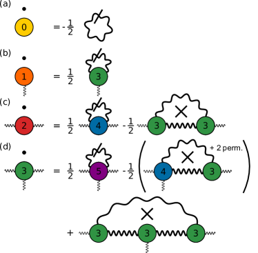
Figure 2: Graphical representation of exact FRG flow equations for the irreducible vertices of effective phonon action (17). (a) Flow equation (54) for the free energy; (b) flow equation (56) for the one-point vertex; (c) flow equation (58) for the two-point vertex; (d) flow equation (60) for the three-point vertex, where “+ 2 perm.” denotes two additional diagrams obtained by exchanging the labels $(Q_{1}\leftrightarrow Q_{2})$ and $(Q_{1}\leftrightarrow Q_{3})$ of the external legs attached to the three-point vertex. The thick wavy lines represent the regularized phonon propagator $\tilde{D}_{\Lambda}(Q)$, while the slash represents the regulator insertion, $-\partial_{\Lambda}R_{\Lambda}(Q)$. A cross inside a loop corresponds to a sum where each propagator of the loop is once slashed according to the product rule (59). A colored circle labeled by the number $n$ represents an $n$-point vertex $\tilde{\Gamma}^{(n)}_{\Lambda}$. The dots above the vertices denote a scale derivative.

III.2 Classification of couplings and flow of relevant couplings

To classify the infinite set of vertices in our scale-dependent average effective phonon action $\tilde{\Gamma}_{\Lambda}[\varphi]$, we note that for small momenta $q\ll k_{F}$ and for frequencies $|\bar{\omega}|\ll v_{F}q$ the two-point vertex is initially given by

$$\tilde{\Gamma}^{(2)}_{\Lambda_{0}}(Q)=r_{0}+b_{0}|\bar{\omega}|/q+c_{0}q^{2}+{\cal{O}}(\bar{\omega}^{2},q^{4}),$$ (61)

where the $r_{0}$, $b_{0}$ and $c_{0}$ are the RPA coefficients given in Eqs. (31). Assuming that this form is not changed by the induced interactions between the phonons, the flowing two-point vertex at scale $\Lambda$ is given by [34]

$$\tilde{\Gamma}^{(2)}_{\Lambda}(Q)=r_{\Lambda}+b_{\Lambda}|\bar{\omega}|/q+c_{\Lambda}q^{2}+{\cal{O}}(\bar{\omega}^{2},q^{4}),$$ (62)

where $r_{\Lambda}$ can be identified with the square of the renormalized phonon frequency at scale $\Lambda$. Note that the correction of order $\bar{\omega}^{2}$ due to the inverse bare propagator is negligible relative to the Landau damping term $b_{0}|\bar{\omega}|/q$ if

$$q\lesssim\sqrt{\lambda_{0}}\frac{{\omega}_{0}}{v_{F}}=\frac{\gamma_{0}\sqrt{\nu}}{v_{F}}\equiv q_{0},$$ (63)

which plays the role of an ultraviolet cutoff in our low-energy theory. In the adiabatic limit $\omega_{0}\ll\epsilon_{F}$ the cutoff $q_{0}$ is small compared with $k_{F}$, while $q_{0}\gg k_{F}$ in the antiadiabatic limit $\omega_{0}\gg\epsilon_{F}$.

If the system exhibits a Pomeranchuk instability then the coupling $r_{\Lambda}$ vanishes for $\Lambda\rightarrow 0$. It is then natural to rescale momenta, frequencies, and the field such that the couplings $b_{\Lambda}$ and $c_{\Lambda}$ are both marginal, which is achieved by rescaling them by the following powers of $\Lambda$,

$$q \propto \Lambda,$$ (64a)

$$\bar{\omega} \propto \Lambda^{z},$$ (64b)

$$\phi_{Q} \propto \Lambda^{-1-\frac{d+z}{2}},$$ (64c)

where we introduce the dynamical exponent

$$z=3.$$ (65)

Note that the powers of $\Lambda$ are simply the canonical dimensions of the corresponding quantities, which can be determined by dimensional analysis. The one-point vertex inherits the canonical scaling of the field,

$$\tilde{\Gamma}^{(1)}_{\Lambda}\propto\Lambda^{-1-\frac{d+z}{2}}=\Lambda^{-\frac{d+5}{2}},$$ (66)

while the three-point and the four-point vertices for vanishing energy-momenta scale as follows,

$$\tilde{\Gamma}^{(3)}_{\Lambda}(0,0,0) \propto \Lambda^{-3+\frac{d+z}{2}}=\Lambda^{\frac{d-3}{2}},$$ (67a)

$$\tilde{\Gamma}^{(4)}_{\Lambda}(0,0,0,0) \propto \Lambda^{-4+d+z}=\Lambda^{d-1}.$$ (67b)

The important point is that the three-point vertex is relevant below three dimensions and therefore cannot be neglected in this case. Keeping in mind that with the dynamic exponent $z=3$ the effective dimensionality is shifted to $d+z=d+3$ [35], the relevance of the three-point vertex in our effective phonon theory is consistent with the well-known fact that in $\phi^{3}$-theory the three-point vertex becomes relevant below six dimensions [36, 37, 38, 39, 40, 41]. To take into account the most relevant interaction processes between the phonons in dimensions $d\leq 3$ we therefore should consider the projected RG flow in the space of the following three couplings,

$$h_{\Lambda} = \tilde{\Gamma}^{(1)}_{\Lambda},$$ (68a)

$$r_{\Lambda} = \tilde{\Gamma}^{(2)}_{\Lambda}(0),$$ (68b)

$$g_{\Lambda} = \tilde{\Gamma}^{(3)}_{\Lambda}(0,0,0).$$ (68c)

Neglecting all other couplings, the exact flow equations (56), (58), and (60) reduce to the following system of truncated flow equations for the relevant couplings,

$$\partial_{\Lambda}h_{\Lambda} = \frac{{g}_{\Lambda}}{2}\int_{Q}\dot{\tilde{D}}_{\Lambda}(Q),$$ (69a)

$$\partial_{\Lambda}{r}_{\Lambda} = -{g}_{\Lambda}^{2}\int_{Q}\dot{\tilde{D}}_{\Lambda}(Q)\tilde{D}_{\Lambda}(Q),$$ (69b)

$$\partial_{\Lambda}{g}_{\Lambda} = 3{g}_{\Lambda}^{3}\int_{Q}\dot{\tilde{D}}_{\Lambda}(Q)\tilde{D}^{2}_{\Lambda}(Q).$$ (69c)

In the following, we will neglect the flow of the marginal couplings $b_{\Lambda}$ and $c_{\Lambda}$ in the low-energy expansion (62), which amounts to neglecting the momentum and frequency dependence of the phonon self-energy, $\Delta_{\Lambda}(Q)\approx\Delta_{\Lambda}(0)$. We thus approximate $b_{\Lambda}\approx b_{0}$ and $c_{\Lambda}\approx c_{0}$, where the initial values $b_{0}$ and $c_{0}$ are given in Eqs. (31b) and (31c). Within this truncation the possibility that the dynamical exponent $z$ is modified by an anomalous dimension is not taken into account. The regularized flowing phonon propagator is then given by

$$\tilde{D}_{\Lambda}(Q)=\frac{1}{r_{\Lambda}+b_{0}|\bar{\omega}|/q+c_{0}q^{2}+R_{\Lambda}(Q)}.$$ (70)

At this point we have to specify the regulator. While the required boundary conditions can be satisfied in many ways, for our purpose it is most convenient to work with a Litim-type regulator [42] adapted to the peculiar momentum and frequency dependence of the bare propagator,

$$R_{\Lambda}(Q)=(c_{0}\Lambda^{2}-b_{0}|\bar{\omega}|/q-c_{0}q^{2})\Theta(c_{0}\Lambda^{2}-b_{0}|\bar{\omega}|/q-c_{0}q^{2}).$$ (71)

The momentum and frequency integrations in our flow equations (69) can then be carried out exactly and we obtain

$$\partial_{\Lambda}h_{\Lambda} = -\frac{2K_{d}}{\pi(d+1)(d+3)}\frac{c_{0}^{2}}{b_{0}}\frac{\Lambda^{d+4}g_{\Lambda}}{(r_{\Lambda}+c_{0}\Lambda^{2})^{2}},$$ (72a)

$$\partial_{\Lambda}r_{\Lambda} = \frac{4K_{d}}{\pi(d+1)(d+3)}\frac{c^{2}_{0}}{b_{0}}\frac{\Lambda^{d+4}g^{2}_{\Lambda}}{(r_{\Lambda}+c_{0}\Lambda^{2})^{3}},$$ (72b)

$$\partial_{\Lambda}g_{\Lambda} = -\frac{12K_{d}}{\pi(d+1)(d+3)}\frac{c^{2}_{0}}{b_{0}}\frac{\Lambda^{d+4}g_{\Lambda}^{3}}{(r_{\Lambda}+c_{0}\Lambda^{2})^{4}},\hskip 19.91692pt$$ (72c)

where $K_{d}$ is the surface area of the $d$-dimensional unit sphere divided by $(2\pi)^{d}$. Introducing the logarithmic flow parameter $l=\ln(\Lambda_{0}/\Lambda)$ and the dimensionless rescaled couplings

$$\tilde{h}_{l} = \frac{h_{\Lambda}}{\sqrt{\frac{K_{d}}{\pi(d+1)(d+3)}}\frac{c_{0}}{\sqrt{b_{0}}}\Lambda^{\frac{d+5}{2}}},$$ (73a)

$$\tilde{r}_{l} = \frac{r_{\Lambda}}{c_{0}\Lambda^{2}},$$ (73b)

$$\tilde{g}_{l} = \sqrt{\frac{4K_{d}}{\pi(d+1)(d+3)}}\frac{\Lambda^{\frac{d-3}{2}}g_{\Lambda}}{c_{0}\sqrt{b_{0}}},$$ (73c)

the flow equations (72) can be written as

$$\partial_{l}\tilde{h}_{l} = \frac{d+5}{2}\tilde{h}_{l}+\frac{\tilde{g}_{l}}{(\tilde{r}_{l}+1)^{2}},$$ (74a)

$$\partial_{l}\tilde{r}_{l} = 2\tilde{r}_{l}-\frac{\tilde{g}_{l}^{2}}{(\tilde{r}_{l}+1)^{3}},$$ (74b)

$$\partial_{l}\tilde{g}_{l} = \frac{3-d}{2}\tilde{g}_{l}+\frac{3\tilde{g}_{l}^{3}}{(\tilde{r}_{l}+1)^{4}}.$$ (74c)

Using the RPA expressions (31) and the initial condition (51) we find that the initial values of our rescaled couplings are

$$\tilde{h}_{0} = \frac{\frac{\rho_{0}(\mu+\delta\mu)}{\nu\epsilon_{F}}-\frac{\delta\mu}{\lambda_{0}\epsilon_{F}}}{\sqrt{\frac{K_{d}C_{d}^{2}}{\pi(d+1)(d+3)B_{d}}}\sqrt{\frac{2k_{F}^{d}}{\nu\epsilon_{F}}}\left(\frac{\Lambda_{0}}{k_{F}}\right)^{\frac{d+5}{2}}},$$ (75a)

$$\tilde{r}_{0} = \frac{1-\lambda_{0}}{C_{d}\lambda_{0}}\left(\frac{k_{F}}{\Lambda_{0}}\right)^{2},$$ (75b)

$$\tilde{g}_{0} = \sqrt{\frac{4K_{d}}{\pi(d+1)(d+3)B_{d}C_{d}^{2}}}\sqrt{\frac{2k_{F}^{d}}{\nu\epsilon_{F}}}\frac{\nu^{\prime}\epsilon_{F}}{\nu}\left(\frac{\Lambda_{0}}{k_{F}}\right)^{\frac{d-3}{2}}.$$

(75c)

Here $\delta\mu=-\gamma_{0}\phi^{0}$ is the shift of the chemical potential due to the finite expectation value of the phonon displacement and $\rho_{0}(\mu+\delta\mu)=\int_{K}\tilde{G}_{0}(K)$ is the density of free electrons at the shifted chemical potential $\mu+\delta\mu$. Note that $\delta\mu$ should be considered as a free parameter which should be adjusted such that the coupling $h_{\Lambda}$ vanishes for $\Lambda\rightarrow 0$, which enforces the boundary condition (50).

III.3 RG flow and Pomeranchuk fixed points in $d>3$

In Fig. 3 we show the RG flow of our effective phonon action obtained from the numerical solution of the flow equations (74) for $d=1,2,3$.

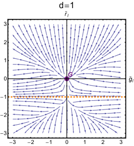
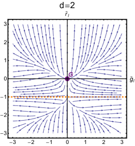
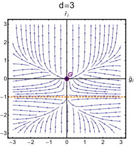
Figure 3: RG flow of the effective phonon action (17) in the $\tilde{g}_{l}-\tilde{r}_{l}$-plane in $d=1,2,3$ obtained from the numerical solution of the flow equations (74). The arrows indicate the direction of the RG flow toward the infrared. For $d\leq 3$ the dimensionless rescaled flow equations have only a trivial, i.e., Gaussian, fixed point $G$, which is represented by a purple dot. A subset of initial values, which exhibit a runaway flow, tend to $\tilde{r}_{\ast}=-1$ which is marked as an orange dashed line.

Obviously, the RG flow has only a trivial Gaussian fixed point $G$ where all couplings vanish; nontrivial fixed points with finite values of rescaled couplings do not exist in $d\leq 3$. We conclude that in and below three dimensions the Holstein model does not have a quantum critical point associated with a Pomeranchuk instability. Note that in a perturbative calculation the relevant three-point vertex which is essential for this result appears only at order $\lambda_{0}^{3}$ so that our calculation to order $\lambda_{0}^{2}$ in Sec. II does not include the relevant critical fluctuations.

However, for $d>3$ we obtain two nontrivial fixed points $P^{+}$ and $P^{-}$ which can be associated with a quantum critical point due to a Pomeranchuk instability. To calculate the couplings $(\tilde{h}_{\ast},\tilde{r}_{\ast},\tilde{g}_{\ast})$ at the fixed points, we set the left-hand sides of the flow equations (74) equal to zero. The fixed-point condition due to the flow equation (69c) for the three-point vertex reads

$$\tilde{g}_{\ast}^{2}=\frac{d-3}{6}(\tilde{r}_{\ast}+1)^{4},$$ (76)

which is valid for $\tilde{g}_{\ast}\neq 0$. This equation has real solutions only for $d>3$, hence a nontrivial fixed point corresponding to a Pomeranchuk instability can only exist in dimensions larger than three. Similarly, the fixed point condition resulting from the flow equation (74b) gives

$$2\tilde{r}_{\ast}=\frac{\tilde{g}_{\ast}^{2}}{(\tilde{r}_{\ast}+1)^{3}}.$$ (77)

Eliminating $\tilde{g}_{\ast}^{2}$ in Eq. (77) using Eq. (76) we obtain an equation for the value of $\tilde{r}_{\ast}$ dependent only on the deviation $\epsilon$ from three dimensions

$$\tilde{r}_{\ast}=\frac{\epsilon}{12-\epsilon},\;\;\;\epsilon=d-3.$$ (78)

Substituting this back into Eq. (76) we get two nontrivial fixed-point values for the three-point vertex in dimensions $d>3$,

$$\tilde{g}_{\ast}^{\pm}=\pm\frac{24\sqrt{6\epsilon}}{(\epsilon-12)^{2}}.$$ (79)

Finally, we combine the fixed point condition resulting from the flow equation (74a) with the previously calculated values $\tilde{r}_{\ast}$ and $\tilde{g}_{\ast}^{\pm}$ to obtain the corresponding fixed-point values of the rescaled one-point vertex

$$\tilde{h}_{\ast}^{\pm} = -\frac{2}{d+5}\frac{\tilde{g}^{\pm}_{\ast}}{(\tilde{r}_{\ast}+1)^{2}}=\mp\sqrt{\frac{2\epsilon}{3(\epsilon+8)}}.$$ (80)

We conclude that for $d>3$ the RG flow of the Holstein model exhibits two nontrivial fixed points $P^{+}=(\tilde{h}_{\ast}^{+},\tilde{r}_{\ast},\tilde{g}_{\ast}^{+})$ and $P^{-}=(\tilde{h}_{\ast}^{-},\tilde{r}_{\ast},\tilde{g}_{\ast}^{-})$. At these fixed points the renormalized phonon frequency vanishes. The uniform compressibility then diverges so that the fixed points describe a quantum critical point associated with a Pomeranchuk instability. The RG flow in $d=4$ is shown in Fig. 4. For smaller $d$ the Pomeranchuk fixed points $P^{-}$ and $P^{+}$ move toward the Gaussian fixed point $G$ until they merge with $G$ in $d=3$.

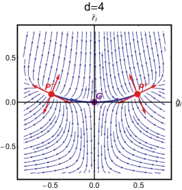
Figure 4: RG flow of the effective phonon action (17) in the $\tilde{g}_{l}-\tilde{r}_{l}$ plane in $d=4$ obtained from the numerical solution of the flow equations (74). In addition to the Gaussian fixed point $G$ there are two nontrivial fixed points $P^{-}$ and $P^{+}$, which are denoted by red dots, corresponding to a Pomeranchuk instability. The two Pomeranchuk fixed points are tricritical, as there are three relevant couplings $\tilde{h}_{l}$, $\tilde{r}_{l}$, and $\tilde{g}_{l}$ whose initial values have to be fine-tuned to reach the fixed point. The eigenvectors of the linearized flow around the Pomeranchuk fixed point are represented by red arrows. Note only the eigenvectors which lie in the $\tilde{g}_{l}$-$\tilde{r}_{l}$-plane are shown. The thick blue line emanates from Pomeranchuck fixed point and flows into the Gaussian fixed point.

From Fig. 4 it is obvious that the Pomeranchuk fixed points in $d>3$ have only relevant directions in our truncated coupling space. Keeping the mind that the arrows on the flow lines indicate the flow toward the infrared (decreasing scale $\Lambda$) the flow toward the ultraviolet (increasing scale) is opposite to the arrows on the flow lines. The Pomeranchuk fixed points are therefore ultraviolet-stable. To calculate the corresponding scaling variables we linearize the flow equations (74) around the fixed points,

$$\partial_{l}\delta\tilde{h}_{l} = \left(4+\frac{\epsilon}{2}\right)\delta\tilde{h}_{l}-\frac{2\tilde{g}_{\ast}\delta\tilde{r}_{l}}{(1+\tilde{r}_{\ast})^{3}}+\frac{\delta\tilde{g}_{l}}{(1+\tilde{r}_{\ast})^{2}},$$ (81a)

$$\partial_{l}\delta\tilde{r}_{l} = \left(2+\frac{3\tilde{g}_{*}^{2}}{(1+\tilde{r}_{*})^{4}}\right)\delta\tilde{r}_{l}-\frac{2\tilde{g}_{*}^{2}}{(1+\tilde{r}_{*})^{3}}\delta\tilde{g}_{l},$$ (81b)

$$\partial_{l}\delta\tilde{g}_{l} = -\frac{12\tilde{g}_{*}^{3}}{(1+\tilde{r}_{*})^{5}}\delta\tilde{r}_{l}-\left(\frac{\epsilon}{2}-\frac{9\tilde{g}_{*}^{2}}{(1+\tilde{r}_{*})^{4}}\right)\delta\tilde{g}_{l}.\hskip 19.91692pt$$ (81c)

The eigenvalues and normalized eigenvectors $\bm{v}=({v}_{h},{v}_{r},{v}_{g})^{T}$ of the linearized flow close to $P^{+}$ are

$$\lambda_{1} =4.5, \bm{v}_{1}^{+}=\begin{pmatrix}-0.843\\ 0.448\\ -0.298\end{pmatrix},$$ (82a)

$$\lambda_{2} =0.641, \bm{v}_{2}^{+}=\begin{pmatrix}0\\ 0.432\\ 0.902\end{pmatrix},$$ (82b)

$$\lambda_{3} =2.860, \bm{v}_{3}^{+}=\begin{pmatrix}0\\ 0.928\\ -0.374\end{pmatrix}.$$ (82c)

The linearized flow close to $P^{-}$ has the same eigenvalues but different eigenvectors which can be obtained by inverting the first and third components of the corresponding $P^{+}$ eigenvectors,

$$\bm{v}_{1}^{-}=\begin{pmatrix}0.843\\ 0.448\\ 0.298\end{pmatrix},\;\;\;\bm{v}_{2}^{-}=\begin{pmatrix}0\\ 0.432\\ -0.902\end{pmatrix},\;\;\;\bm{v}_{3}^{-}=\begin{pmatrix}0\\ 0.928\\ 0.374\end{pmatrix}.$$ (83)

Since all three eigenvalues are positive both fixed points $P^{+}$ and $P^{-}$ are tricritical. The eigendirections are indicated by red arrows in Fig. 4. For completeness, we also show in Fig. 5 the projections of the RG flow in $d=4$ onto the $\tilde{g}$ -$\tilde{h}$ plane at $\tilde{r}_{l}=\tilde{r}_{\ast}$ and the $\tilde{r}$-$\tilde{h}$ plane at $\tilde{g}_{l}=\tilde{g}^{+}_{\ast}$ and $\tilde{g}_{l}=\tilde{g}^{-}_{\ast}$, respectively.

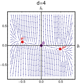
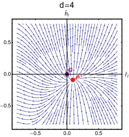
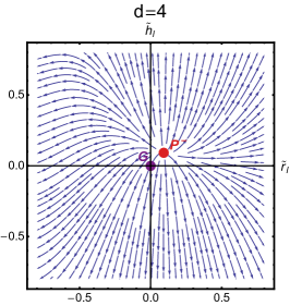
Figure 5: RG flow of the effective phonon action (17) in $d=4$ obtained from the numerical solution of the flow equations (74). Left: RG flow in the $\tilde{g}_{l}$ - $\tilde{r}_{l}$ plane at $\tilde{r}=\tilde{r}_{\ast}$. Middle: RG flow in the $\tilde{r}_{l}$ - $\tilde{h}_{l}$ plane at $\tilde{g}_{l}=\tilde{g}^{+}_{\ast}$. Right: RG flow in the $\tilde{r}_{l}$ - $\tilde{h}_{l}$ plane at $\tilde{g}_{l}=\tilde{g}^{-}_{\ast}$.

Recall that the relevant coupling $\tilde{h}_{l}$ is related to the renormalized one-point vertex of our effective phonon action and is related to the shift in the chemical potential which is necessary to keep the density constant; see Eqs. (51). Note that $\tilde{h}_{l}$ is exactly analogous to an external magnetic field in the Ginzburg-Landau-Wilson Hamiltonian for the Ising model [43]. The existence of a pair of nontrivial ultraviolet-stable fixed points in our effective phonon theory for the Holstein model defined by the Euclidean action $S_{\rm eff}[X]$ in Eq. (17) is closely related to a similar pair of fixed points of scalar $\phi^{3}$-theory above six dimensions [36, 37, 38, 39]. The shift in the dimensionality is due to the fact that the quantum action $S_{\rm eff}[X]$ is characterized by a dynamical exponent $z=3$ so that the critical dimension above which these fixed points emerge is reduced from six to $6-z=3$, see Ref. [35]. Note that in the context of $\phi^{3}$-theory the ultraviolet-stable nontrivial fixed points above six dimensions have recently received renewed interest in high-energy physics [40, 41] because these fixed points offer a possibility to construct a well-defined continuum limit of perturbatively nonrenormalizable field theories (asymptotic safety [44, 45]).

Next, let us discuss the implications of our RG analysis for the phase diagram of the Holstein model. From the flow diagrams in Figs. 3, 4, and 5 it is clear that in all dimensions the RG flow of the Holstein model in the $\tilde{g}$ - $\tilde{r}$-plane is divided by a separatrix into two regimes. In the first regime $\tilde{r}_{l}$ flows to positive values so that the renormalized phonon frequency is finite. Since we do not take into account possible superfluid states, the ground state is then expected to be a normal Fermi liquid. In the second regime $\tilde{r}_{l}$ flows to negative values and eventually diverges at a finite scale $\Lambda_{*}$. The interpretation of this runaway flow is somewhat ambiguous so that we need information from other methods to draw conclusions for the phase diagram. In two dimensions various numerical calculations [4, 6, 7, 8, 10] found that for sufficiently strong electron-phonon coupling the Holstein model exhibits a first-order transition from a Fermi liquid (FL) phase to a charge-density-wave (CDW) phase. In addition, some authors [6] also found that in a certain interval of densities and for not too large values of the adiabatic ratio $\omega_{0}/\epsilon_{F}$ the system phase separates (PS) into regions with different densities. The transition between the FL and CDW as well as the transition between the FL and the PS phase are first order. The fact that in the antiadiabatic limit $\omega_{0}\gg\epsilon_{F}$ the FL phase becomes unstable towards a CDW can also understood by considering the effective electronic action obtained by integrating over the phonons,

$$S_{\rm eff}[\bar{c},c]=-\int_{K}G_{0}^{-1}(K)\bar{c}_{K}c_{K}-\frac{\gamma_{0}^{2}}{2}\int_{Q}D_{0}(Q)\rho_{-Q}\rho_{Q},$$ (84)

where $\rho_{Q}=\int_{K}\bar{c}_{K}c_{K+Q}$ represents the electronic density. In the antiadiabatic limit the free phonon propagator can be approximated by $D_{0}(Q)\approx 1/\omega_{0}^{2}$ so that the last term in Eq. (84) reduces to a local attractive interaction with strength $-\gamma_{0}^{2}/\omega_{0}^{2}=-\lambda_{0}/\nu$. For not too small densities the dominant instability of this model is expected to be CDW [10, 46]. Assuming that the phase diagram of the Holstein model in $d=3$ is not qualitatively different from the phase diagram in $d=2$ (this assumption is supported by Fig. 3 which shows qualitatively similar RG flows in $d=3$ and $d=2$), we propose that in three dimensions the phase diagram of the Holstein model as a function of the electron-phonon coupling $\lambda_{0}$ and the adiabatic ratio $\omega_{0}/\epsilon_{F}$ has for fixed, but not too small, densities the form sketched in Fig. 6. Here all phase boundaries are first order and the intersection of the three phase boundaries is not a critical point but a triple point because for $d\leq 3$ our RG analysis rules out a critical point with a divergent uniform compressibility.

However, for $d>3$ we expect that the intersection of the three phase boundaries in Fig. 6 becomes a critical point. The critical behavior close to this point is then controlled by one of the Pomeranchuk fixed points discussed above. The phase boundary between the FL and the PS phase is still first order, because we know that both the adiabatic ratio $\omega_{0}/\epsilon_{F}$ and the electron-phonon coupling $\lambda_{0}$ have to be fine-tuned to obtain criticality. The nature of the other phase boundaries remains to be investigated, but this is beyond the scope of this work.

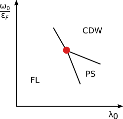
Figure 6: Schematic ground state phase diagram of the Holstein model in $d=3$ in the plane spanned by the electron-phonon coupling $\lambda_{0}$ and the adiabatic ratio $\omega_{0}/\epsilon_{F}$ for fixed but not too small densities. We have ignored a possible superfluid phase, assuming that the weak-coupling phase is a normal Fermi liquid (FL). In the adiabatic regime $\omega_{0}/\epsilon_{F}\ll 1$ we expect a first-order transition to a phase-separated (PS) inhomogeneous state when $\lambda_{0}$ exceeds a certain threshold of order unity. However, in the antiadiabatic regime $\omega_{0}/\epsilon_{F}\gg 1$ there is a first-order transition to a state with charge-density-wave (CDW) order. In $d\leq 3$ the intersection of the three phase boundaries (red dot) is a noncritical triple point. For $d>3$ the triple point transforms into a critical point while the phase boundary between the FL and the PS phases remains first order.

IV Summary and conclusions

In this work we have presented evidence that in dimensions $d>3$ the Holstein model exhibits a quantum critical point associated with a Pomeranchuk instability. The underlying critical RG fixed point is ultraviolet stable and can only be realized if both the dimensionless electron-phonon coupling $\lambda_{0}$ and the adiabatic ratio $\omega_{0}/\epsilon_{F}$ are fine-tuned. This fixed point is closely related to the well-known ultraviolet-stable fixed point of $\phi^{3}$-theory above six dimensions; the dynamic exponent $z=3$ reduces the relevant critical dimension from six to three. Note that the bare value of the relevant three-point vertex in our effective phonon action is proportional to the third power $\lambda_{0}^{3}$ of dimensionless electron-phonon coupling so that second-order perturbation theory in $\lambda_{0}$ is not sufficient to detect the singularities associated with the dominant critical fluctuations. Our result that for $d\leq 3$ the RG flow of Holstein model does not have a nontrivial fixed point associated with a Pomeranchuk instability does not exclude the possibility that the phase diagram contains regimes where the state of the system exhibits phase separation. However, the transitions to this state must be first order. By combining our RG analysis with numerical results for the phase diagram of the two-dimensional Holstein model by other authors [4, 6, 7, 8, 10] we propose the schematic phase diagram of the Holstein model shown in Fig. 6.

For our calculation of the compressibility we have used the exact Ward identity (6) to express the compressibility in terms of the renormalized phonon frequency of the Holstein model. For our purpose, it is therefore sufficient to analyze the effective phonon action $S_{\rm eff}[X]$ defined in Eq. (17). Unfortunately, the renormalized electron-phonon vertex cannot be calculated within this approach so that we cannot make statements about the validity of Migdal’s theorem close the Pomeranchuk instability. In principle our FRG approach can be generalized to obtain also flow equations for the electron-phonon vertices, but this is beyond the scope of this work.

Finally, let us comment on the significance of our finding that the Pomeranchuk fixed points of the Holstein model in $d>3$ are ultraviolet stable. RG fixed points with this property are crucial to define a well-defined continuum limit in perturbatively nonrenormalizable field theories. If these fixed points are non-Gaussian, the theory is called asymptotically safe, a prominent candidate being quantum gravity [44], where evidence for the existence of a nontrivial ultraviolet-stable fixed point has been obtained by means of FRG methods [45, 21]. In this sense, the effective phonon action of the Holstein model in $d>3$ defines an asymptotically save field theory. However, for $d\leq 3$ the ultraviolet-stable fixed point of the Holstein model is Gaussian so that the interaction vanishes at the fixed point (asymptotic freedom). Of course, the effective phonon action of the Holstein model has an intrinsic ultraviolet cutoff given by $q_{0}$ defined in Eq. (63), but for all RG trajectories which emanate from the UV-stable fixed points the UV cutoff can be removed without affecting any physical observables.

APPENDIX A: Dyson-Schwinger equations and Ward identities for the Holstein model

The renormalized phonon frequency in the Holstein model is related to the compressibility via the Ward identity (6) which is closely related to the well-known compressibility sum rule [33, 47, 48]. The specific form of this Ward identity for the Holstein model apparently cannot be found in the literature. In this Appendix we therefore give a self-contained derivation of Eq. (6) and related Ward identities using functional methods.

.1 Dyson-Schwinger equations

To begin with, we derive Dyson-Schwinger equations (also called skeleton equations) for the Holstein model, relating correlation functions of different order. Therefore we follow the method outlined in Refs. [19, 49]. Consider the generating functional of the Euclidean correlation functions of the Holstein model,

$${\cal{G}}[\bar{\eta},\eta,J]=\int{\cal{D}}[\bar{c},c,X]e^{-S+(\bar{\eta},c)+(\bar{c},\eta)+(J,X)},$$ (A1)

where $\bar{\eta}$ and $\eta$ are Grassmann sources, $J$ is a bosonic source field, and we have used the abbreviations

$$(\bar{\eta},c)+(\bar{c},\eta) = \int_{K}(\bar{\eta}_{K}c_{K}+\bar{c}_{K}\eta_{K}),$$ (A2)

$$(J,X) = \int_{Q}J_{-Q}X_{Q}.$$ (A3)

The Euclidean bare action $S[\bar{c},c,X]$ of the Holstein model is given in Eq. (7). Using the invariance of the functional integral in Eq. (A1) with respect to infinitesimal shifts in the integration variables we obtain the functional equations

$$\left(J_{-Q}-D_{0}^{-1}(Q)\frac{\delta}{\delta J_{Q}}\right){\cal{G}}-\zeta\gamma_{0}\int_{K}\frac{\delta^{2}{\cal{G}}}{\delta\eta_{K+Q}\delta\bar{\eta}_{K}} = 0,$$

$$\left(\zeta\bar{\eta}_{K}-\bar{G}_{0}^{-1}(K)\frac{\delta}{\delta\eta_{K}}\right){\cal{G}}-\gamma_{0}\int_{Q}\frac{\delta^{2}{\cal{G}}}{\delta\eta_{K+Q}\delta J_{-Q}} = 0,$$

$$\left({\eta}_{K}-\bar{G}_{0}^{-1}(K)\frac{\delta}{\delta\bar{\eta}_{K}}\right){\cal{G}}-\gamma_{0}\int_{Q}\frac{\delta^{2}{\cal{G}}}{\delta\bar{\eta}_{K-Q}\delta J_{-Q}} = 0,$$

where $\bar{G}_{0}(K)=-G_{0}(K)$ and we have introduced the fermionic statistics factor $\zeta=-1$. Next, we express the above Dyson Schwinger equations in terms of the generating functional of connected correlation functions

$${\cal{G}}_{c}[\bar{\eta},\eta,J]=\ln{\cal{G}}[\bar{\eta},\eta,J],$$ (A5)

and its subtracted Legendre transform

$$\Gamma[\bar{\psi},\psi,\phi]=(\bar{\eta},\psi)+(\bar{\psi},\eta)+(J,\phi)-{\cal{G}}_{c}[\bar{\eta},\eta,J]$$

$$-\int_{K}\bar{G}_{0}^{-1}(K)\bar{\psi}_{K}\psi_{K}-\frac{1}{2}\int_{Q}D_{0}^{-1}(Q)\phi_{-Q}\phi_{Q},$$ (A6)

where on the right-hand side the sources should be expressed in terms of the field expectation values by inverting the relations

$$\frac{\delta{\cal{G}}_{c}}{\delta\bar{\eta}_{K}} = \psi_{K}=\langle c_{K}\rangle,$$ (A7a)

$$\frac{\delta{\cal{G}}_{c}}{\delta{\eta}_{K}} = \zeta\bar{\psi}_{K}=\zeta\langle\bar{c}_{K}\rangle,$$ (A7b)

$$\frac{\delta{\cal{G}}_{c}}{\delta J_{-Q}} = \phi_{Q}=\langle X_{Q}\rangle.$$ (A7c)

Note that by construction

$$\frac{\delta\Gamma}{\delta\bar{\psi}_{K}}+\bar{G}_{0}^{-1}(K)\psi_{K} = \eta_{K},$$ (A8a)

$$\frac{\delta\Gamma}{\delta{\psi}_{K}}+\zeta\bar{G}_{0}^{-1}(K)\bar{\psi}_{K} = \zeta\bar{\eta}_{K},$$ (A8b)

$$\frac{\delta\Gamma}{\delta\phi_{-Q}}+D_{0}^{-1}(Q)\phi_{Q} = J_{Q}.$$ (A8c)

The Dyson-Schwinger equations (A4) then reduce to

$$\frac{\delta\Gamma}{\delta\phi_{Q}}-\gamma_{0}\int_{K}\left(\bar{\psi}_{K+Q}\psi_{K}+\frac{\delta^{2}{\cal{G}}_{c}}{\delta\bar{\eta}_{K}\delta\eta_{K+Q}}\right) = 0,\hskip 19.91692pt$$ (A9a)

$$\frac{\delta\Gamma}{\delta\psi_{K}}-\gamma_{0}\int_{Q}\left(\zeta\bar{\psi}_{K+Q}\phi_{Q}+\frac{\delta^{2}{\cal{G}}_{c}}{\delta{\eta}_{K+Q}\delta J_{-Q}}\right) = 0,\hskip 28.45274pt$$ (A9b)

$$\frac{\delta\Gamma}{\delta\bar{\psi}_{K}}-\gamma_{0}\int_{Q}\left({\psi}_{K-Q}\phi_{Q}+\frac{\delta^{2}{\cal{G}}_{c}}{\delta\bar{\eta}_{K-Q}\delta J_{-Q}}\right) = 0.$$ (A9c)

By taking successive derivatives of Eqs. (A9) with respect to the field expectation values and then setting the sources equal to zero we obtain an infinite set of Dyson-Schwinger equations for the irreducible vertices.

First of all, let us consider Eq. (A9a) for vanishing sources, taking into account that for finite density the expectation value $\phi_{Q}$ of the phonon field has a finite limit $\phi_{Q}^{0}$. Here the superscript means that $\phi^{0}_{Q}=\langle X_{Q}\rangle$ is calculated for vanishing sources $\eta=\bar{\eta}=J=0$. Using Eq. (A8c) we obtain

$$D_{0}^{-1}(-Q)\phi^{0}_{-Q} = -\gamma_{0}\int_{K}\left.\frac{\delta^{2}{\cal{G}}_{c}}{\delta\bar{\eta}_{K}\delta\eta_{K+Q}}\right|_{\eta=\bar{\eta}=J=0}$$ (A10)

$$= -\gamma_{0}\delta(Q)\int_{K}G(K).$$

The integral $\int_{K}G(K)=\rho$ can be identified with the exact electronic density of the system so that we can write

$$\phi^{0}_{Q}=\delta(Q){\phi^{0}},\;\;\;\;\;\;\phi^{0}=-\frac{\gamma_{0}}{\omega_{0}^{2}}\rho.$$ (A11)

We conclude that for any finite electronic density the phonon displacement field of the Holstein model has a finite expectation value.

Next, we derive the Dyson-Schwinger equation for the electronic self-energy. Applying $\frac{\delta}{\delta\psi_{K}^{\prime}}$ to both sides of Eq. (A9c) and then setting all sources equal to zero gives

$$\delta(K-K^{\prime})\Sigma(K)=\gamma_{0}\phi^{0}_{K-K^{\prime}}$$

$$+\gamma_{0}\left.\int_{Q}\frac{\delta^{3}{\cal{G}}_{c}}{\delta\psi_{K^{\prime}}\delta\bar{\eta}_{K-Q}\delta J_{-Q}}\right|_{\eta=\bar{\eta}=J=0}.$$ (A12)

The last term can be expressed in terms of irreducible vertices as follows [19, 49],

$$\left.\frac{\delta^{3}{\cal{G}}_{c}}{\delta\psi_{K^{\prime}}\delta\bar{\eta}_{K-Q}\delta J_{-Q}}\right|_{\eta=\bar{\eta}=J=0}=\delta(K-K^{\prime})G(K-Q)$$

$$\hskip 56.9055pt\times\Gamma^{\bar{c}c\varphi}(K-Q,K,-Q)D(-Q),\hskip 19.91692pt$$ (A13)

where the three-legged vertex $\Gamma^{\bar{c}c\varphi}(K+Q,K,Q)$ is defined by expanding the functional $\Gamma[\bar{\psi},\psi,\phi]$ around $\phi=\phi^{0}$, i.e.,

$$\Gamma[\bar{\psi},\psi,\phi^{0}+\varphi]=\Gamma[0,0,\phi^{0}]-\gamma_{0}\rho\varphi_{Q=0}$$

$$+\int_{K}\Sigma(K)\bar{\psi}_{K}\psi_{K}+\frac{1}{2}\int_{Q}\Delta(Q)\varphi_{-Q}\varphi_{Q}$$

$$+\int_{K}\int_{Q}\Gamma^{\bar{c}c\varphi}(K+Q,K,Q)\bar{\psi}_{K+Q}\psi_{K}\varphi_{Q}+\ldots\;.\hskip 19.91692pt$$ (A14)

Note that the vertex expansion of the Legendre transform

$${\cal{L}}[\bar{\psi},\psi,\phi]=(\bar{\eta},\psi)+(\bar{\psi},\eta)+(J,\phi)-{\cal{G}}_{c}[\bar{\eta},\eta,J]$$

$$={\Gamma}[\bar{\psi},\psi,\phi]+\int_{K}\bar{G}_{0}^{-1}(K)\bar{\psi}_{K}\psi_{K}+\frac{1}{2}\int_{Q}D_{0}^{-1}(Q)\phi_{-Q}\phi_{Q}$$

does not have a linear term,

$${\cal{L}}[\bar{\psi},\psi,\phi^{0}+\varphi]={\cal{L}}[0,0,\phi^{0}]$$

$$-\int_{K}G^{-1}(K)\bar{\psi}_{K}\psi_{K}+\frac{1}{2}\int_{Q}D^{-1}(Q)\varphi_{-Q}\varphi_{Q}$$

$$+\int_{K}\int_{Q}\Gamma^{\bar{c}c\varphi}(K+Q,K,Q)\bar{\psi}_{K+Q}\psi_{K}\varphi_{Q}+\ldots\;.\hskip 19.91692pt$$ (A16)

Here the exact electron and phonon propagators can be expressed via the corresponding self-energies $\Sigma(K)$ and $\Delta(Q)$ via the Dyson equations

$$G(K) = \frac{1}{i\omega-\epsilon_{\bm{k}}+\mu-\Sigma(K)},$$ (A17)

$$D(Q) = \frac{1}{\bar{\omega}^{2}+\omega_{0}^{2}+\Delta(Q)}.$$ (A18)

The Dyson-Schwinger equation for the electronic self-energy can then be written as

$$\Sigma(K)=\gamma_{0}\phi^{0}$$

$$+\gamma_{0}\int_{Q}D(Q)G(K+Q)\Gamma^{\bar{c}c\varphi}(K+Q,K,Q),$$ (A19)

which is shown diagrammatically in Fig. 7 (a).

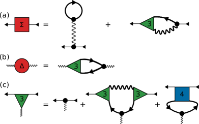
Figure 7: Diagrammatic representation of Dyson-Schwinger equations for the Holstein model: (a) electronic self-energy, (b) phonon self-energy, and (c) electron-phonon vertex (represented by a green triangle). The solid arrows represent the exact electron propagator $G(K)$ and the thick wavy lines represent the exact phonon propagator $D(Q)$. The thin wavy line in the tadpole contribution to the electronic self-energy represents the bare static phonon propagator $D_{0}(0)=1/\omega_{0}^{2}$. The bare phonon vertex $\gamma_{0}$ is represented by a black dot and the irreducible fermionic two-body interaction $\Gamma^{\bar{c}\bar{c}cc}(K+Q,K^{\prime},K^{\prime}+Q,K)$ is represented by a blue square.

The first term

$$\Sigma_{\rho}=\gamma_{0}\phi^{0}=-\gamma_{0}^{2}D_{0}(0)\rho=-\frac{\gamma_{0}^{2}}{\omega_{0}^{2}}\rho$$ (A20)

can be identified with the sum of all tadpole contributions to the irreducible electronic self-energy. To leading order in the interaction, this is the Hartree correction. The negative sign of the Hartree self-energy can be simply understood from the fact the effective interaction between the electrons mediated by the phonons is attractive for small momentum and energy transfers. To see this, we integrate the exponentiated Euclidean action $e^{-S}$ over the phonon field to obtain that the effective electronic action of the Holstein model, given in Eq. (84), has an attractive two-body interaction $-\gamma_{0}^{2}D_{0}(0)=-\gamma_{0}^{2}/\omega_{0}^{2}$ in the limit of vanishing energy-momentum transfer $Q=0$.

Next, by taking the derivative $\frac{\delta}{\delta\phi_{-Q}}$ of Eq. (A9a) and then taking the limit of vanishing sources we obtain the Dyson-Schwinger equation for the phonon self-energy,

$$\Delta(Q)=\gamma_{0}\int_{K}G(K)G(K+Q)\Gamma^{\bar{c}c\varphi}(K+Q,K,Q),$$ (A21)

which is shown diagrammatically in Fig. 7 (b). Finally, applying $\frac{\delta^{2}}{\delta\bar{\psi}_{K+Q}\delta\psi_{K}}$ to both sides of Eq. (A9a) and then setting the sources equal to zero we obtain the Dyson-Schwinger equation for the electron-phonon vertex

$$\Gamma^{\bar{c}c\varphi}(K+Q,K,Q) = \gamma_{0}+\gamma_{0}\int_{K^{\prime}}G(K^{\prime})G(K^{\prime}+Q)\Bigl{\{}\Gamma^{\bar{c}\bar{c}cc}(K+Q,K^{\prime},K^{\prime}+Q,K)$$ (A22)

$$\hskip 45.5244pt+\Gamma^{\bar{c}c\varphi}(K+Q,K^{\prime}+Q,K-K^{\prime})D(K^{\prime}-K)\Gamma^{\bar{c}c\varphi}(K^{\prime},K,K^{\prime}-K)\Bigr{\}},$$

which is shown diagrammatically in Fig. 7 (c). Here $\Gamma^{\bar{c}\bar{c}cc}(K+Q,K^{\prime},K^{\prime}+Q,K)$ is the effective two-body interaction between the fermions which is irreducible with respect to cutting a single electron line or a single phonon line.

.2 Ward identities

We now show that for $Q=0$ the phonon self-energy can be expressed in terms of the compressibility $\partial\rho/\partial\mu$ via the Ward identity

$$\Delta(0)=-\frac{\gamma_{0}^{2}\frac{\partial\rho}{\partial\mu}}{1+\frac{\gamma_{0}^{2}}{\omega_{0}^{2}}\frac{\partial\rho}{\partial\mu}}.$$ (A23)

For $Q=0$ this implies that the inverse phonon propagator is given by

$$D^{-1}(0)\equiv\tilde{\omega}_{0}^{2}=\omega_{0}^{2}+\Delta(0)=\frac{\omega_{0}^{2}}{1+\frac{\gamma_{0}^{2}}{\omega_{0}^{2}}\frac{\partial\rho}{\partial\mu}},$$ (A24)

which is the Ward identity (6). Note that thermodynamic stability implies that the compressibility is nonnegative so that $D^{-1}(0)\geq 0$. The identities (A23) and (A24) imply that the phonon self-energy $\Delta(0)$ of the Holstein model is strictly negative as long as the normal state is thermodynamically stable. At the same time the renormalized phonon energy is strictly positive and vanishes only when the compressibility diverges.

The identity (A23) is closely related to the fact that for $Q=0$ (more precisely: in the so-called $\bm{q}$-limit where we first set $\bar{\omega}=0$ and then take the limit $\bm{q}\rightarrow 0$) the exact electron-phonon vertex $\Gamma^{\bar{c}c\varphi}(K,K,0)$ satisfies the following Ward identity,

$$\frac{\Gamma^{\bar{c}c\varphi}(K,K,0)}{\gamma_{0}}=\frac{1-\frac{\partial\Sigma(K)}{\partial\mu}}{1-\frac{\partial\Sigma_{\rho}}{\partial\mu}}=\frac{1-\frac{\partial\Sigma(K)}{\partial\mu}}{1+\frac{\gamma_{0}^{2}}{\omega_{0}^{2}}\frac{\partial\rho}{\partial\mu}}.$$ (A25)

Note that if we approximate the self-energy $\Sigma(K)$ by its tadpole contribution $\Sigma_{\rho}$ the vertex $\Gamma^{\bar{c}c\varphi}(K,K,0)$ is not renormalized.

To prove the Ward identity (A25), we use the exact FRG flow equation for the fermionic self-energy in the chemical potential cutoff scheme [50], which for the Holstein model is given by

$$\frac{\partial\Sigma(K)}{\partial\mu}=\Gamma^{\bar{c}c\varphi}(K,K,0)\frac{\partial\phi^{0}}{\partial\mu}-I(K),$$ (A26)

with

$$I(K)=\int_{K^{\prime}}G^{2}(K^{\prime})\Bigl{\{}\Gamma^{\bar{c}\bar{c}cc}(K,K^{\prime},K^{\prime},K)$$

$$+\Gamma^{\bar{c}c\varphi}(K,K^{\prime},K-K^{\prime})D(K^{\prime}-K)\Gamma^{\bar{c}c\varphi}(K^{\prime},K,K^{\prime}-K)\Bigr{\}}.$$

(A27)

However, for $Q=0$ the Dyson-Schwinger equation (A22) for the electron-phonon vertex can be written as

$$\Gamma^{\bar{c}c\varphi}(K,K,0)=\gamma_{0}+\gamma_{0}I(K).$$ (A28)

Using this to eliminate $I(K)$ in the flow equation (A26) we obtain

$$\Gamma^{\bar{c}c\varphi}(K,K,0)=\gamma_{0}+\gamma_{0}\left[\Gamma^{\bar{c}c\varphi}(K,K,0)\frac{\partial\phi^{0}}{\partial\mu}-\frac{\partial\Sigma(K)}{\partial\mu}\right].$$ (A29)

Solving for $\Gamma^{\bar{c}c\varphi}(K,K,0)$ and noting that $\gamma_{0}\phi^{0}=\Sigma_{\rho}$ we obtain the Ward identity (A25). This identity implies the so-called compressibility sum rule [33], which for the Holstein model has the form

$$\frac{\partial\rho}{\partial\mu}\equiv\frac{\partial}{\partial\mu}\int_{K}G(K)=\frac{\Pi(0)}{1-\gamma_{0}^{2}D_{0}(0)\Pi(0)},$$ (A30)

where $\Pi(0)=\lim_{\bm{q}\rightarrow 0}\Pi(\bm{q},i\omega=0)$ is the so-called $\bm{q}$-limit of the irreducible polarization $\Pi(Q)$. The latter satisfies the Dyson-Schwinger equation

$$\Pi(Q)=-\gamma_{0}^{-1}\int_{K}G(K)G(K+Q)\Gamma^{\bar{c}c\varphi}(K+Q,K,Q)$$ (A31)

and is related to the phonon self-energy via

$$\Delta(Q)=-\gamma_{0}^{2}\Pi(Q).$$ (A32)

Setting $Q=0$ in the Dyson-Schwinger equation (A31) and substituting the result into Eq. (A30) we then obtain

$$\frac{\partial\rho}{\partial\mu} = -\int_{K}\left(1-\frac{\partial\Sigma(K)}{\partial\mu}\right)G^{2}(K)$$ (A33)

$$= -\left(1-\frac{\partial\Sigma_{\rho}}{\partial\mu}\right)\frac{1}{\gamma_{0}}\int_{K}\Gamma^{\bar{c}c\varphi}(K,K,0)G^{2}(K).\hskip 19.91692pt$$

The Ward identity (A25) guarantees that this relation is indeed satisfied. By inverting the chain of identities leading from Eq. (A30) to Eq. (A33), we conclude that our Ward identity (A25) is equivalent to the compressibility sum rule (A30).

Finally, to proof the Ward identity (A23), we multiply both sides of Eq. (A30) by $\gamma_{0}^{2}D_{0}(0)$ and use the fact that $\Sigma_{\rho}=-\gamma_{0}^{2}D_{0}(0)\rho$ is the tadpole contribution to the electronic self-energy. We then obtain

$$-\gamma_{0}^{2}D_{0}(0)\Pi(0)=\frac{\frac{\partial\Sigma_{\rho}}{\partial\mu}}{1-\frac{\partial\Sigma_{\rho}}{\partial\mu}},$$ (A34)

which can also be written as

$$1-\gamma_{0}^{2}D_{0}(0)\Pi(0)=\frac{1}{1-\frac{\partial\Sigma_{\rho}}{\partial\mu}},$$ (A35)

and implies

$$\Delta(0)=\omega_{0}^{2}\frac{\frac{\partial\Sigma_{\rho}}{\partial\mu}}{1-\frac{\partial\Sigma_{\rho}}{\partial\mu}},$$ (A36)

which is equivalent with Eq. (A23). Note that with the help of Eq. (A35) the Ward identity (A25) for the electron-phonon vertex can alternatively be written as

$$\frac{\Gamma^{\bar{c}c\varphi}(K,K,0)}{\gamma_{0}} = \left[1-\frac{\gamma_{0}^{2}}{\omega_{0}^{2}}\Pi(0)\right]\left[1-\frac{\partial\Sigma(K)}{\partial\mu}\right]$$ (A37)

$$= \frac{\tilde{\omega}_{0}^{2}}{\omega_{0}^{2}}\left[1-\frac{\partial\Sigma(K)}{\partial\mu}\right].$$

This identity expresses the electron-phonon vertex at vanishing phonon momentum and energy in terms of the square of renormalized phonon frequency $\tilde{\omega}_{0}^{2}=\omega_{0}^{2}+\Delta(0)$ and the derivative of the electronic self-energy with respect to the chemical potential.

APPENDIX B: Symmetrized closed fermion loops

The vertices in the effective phonon action $S_{\rm eff}[X]$ defined in Eq. (21) can be expressed in terms of the symmetrized closed fermion loops $L_{S}^{(n)}(Q_{1},\ldots,Q_{n})$ as given by Eq. (24). The symmetrized closed fermion $n$-loop is defined by

$$L_{S}^{(n)}(Q_{1},\ldots,Q_{n})=\frac{1}{n!}\sum_{P(1,\ldots,n)}L^{(n)}(Q_{P(1)},\ldots,Q_{P(n)}),$$ (B1)

where the sum is over the $n!$ permutations of the labels and $L^{(n)}(Q_{1},\ldots,Q_{n})$ is the corresponding nonsymmetrized loop. To define the latter, we introduce shifted labels $\bar{Q}_{j}=\sum_{i=1}^{j-1}Q_{i}$, i.e.,

$$\bar{Q}_{1} = 0,$$

$$\bar{Q}_{2} = Q_{1},$$

$$\bar{Q}_{3} = Q_{1}+Q_{2},$$

$$\vdots$$

$$\bar{Q}_{n} = Q_{1}+\ldots+Q_{n-1}.$$

The nonsymmetrized loop can then be written as

$$L^{(n)}(Q_{1},\ldots,Q_{n})=\bar{L}^{(n)}(\bar{Q}_{1},\ldots,\bar{Q}_{n}),$$ (B3)

with

$$\bar{L}^{(n)}(\bar{Q}_{1},\ldots,\bar{Q}_{n})=\int_{K}\prod_{i=1}^{n}G_{0}(K-\bar{Q}_{i})$$

$$=\int_{\bm{k}}T\sum_{\omega}G_{0}(K-\bar{Q}_{1})\cdots G_{0}(K-\bar{Q}_{n}).\hskip 19.91692pt$$ (B4)

Here $\int_{K}=\int_{\bm{k}}T\sum_{\omega}$ and $\int_{\bm{k}}=\int\frac{d^{d}k}{(2\pi)^{d}}$ denotes the $d$-dimensional momentum integration. If we set all external momenta equal to zero, then we obtain [51]

$$\bar{L}^{(n)}(0,\ldots,0)=\int_{K}[G_{0}(K)]^{n}=\frac{1}{(n-1)!}\frac{\partial^{n-1}\rho_{0}(\mu)}{\partial\mu^{n-1}},$$ (B5)

where

$$\rho_{0}(\mu)=\int_{K}G_{0}(K)=\int\frac{d^{d}k}{(2\pi)^{d}}\frac{1}{e^{\beta(\epsilon_{\bm{k}}-\mu)}+1}$$ (B6)

is the density of noninteracting electrons as a function of the chemical potential. In particular, at zero temperature

$$\bar{L}^{(2)}(0,0) = -\nu(\mu),$$ (B7)

$$\bar{L}^{(3)}(0,0,0) = \frac{1}{2}\frac{\partial\nu(\mu)}{\partial\mu},$$

$$\vdots$$

$$\bar{L}^{(n)}(0,\ldots,0) = \frac{(-1)^{n-1}}{(n-1)!}\frac{\partial^{n-2}\nu(\mu)}{\partial\mu^{n-2}},$$ (B9)

where

$$\nu(\mu)=\int\frac{d^{d}k}{(2\pi)^{d}}\delta(\mu-\epsilon_{\bm{k}})$$ (B10)

is the density of states at the chemical potential.

References

- [1] A. B. Migdal, Interaction between electrons and lattice vibrations in a normal metal, Zh. Eksp. Teor. Fiz. 34, 1438 (1958) [Sov. Phys. JETP 7, 996 (1958)].
- [2] A. A. Abrikosov, Fundamentals of the Theory of Metals, (North Holland, Amsterdam, 1988).
- [3] G. D. Mahan, Many-Particle Physics, 3rd ed. (Kluwer Academic/Plenum Publishers, New York, NY, 2000).
- [4] S. Kumar and J. van den Brink, Charge ordering and magnetism in quarter-filled Hubbard-Holstein model, Phys. Rev. B 78, 155123 (2008).
- [5] Y. Murakami, P. Werner, N. Tsuji, and H. Aoki, Supersolid Phase Accompanied by a Quantum Critical Point in the Intermediate Coupling Regime of the Holstein Model, Phys. Rev. Lett. 113, 266404 (2014).
- [6] T. Ohgoe and M. Imada, Competition among Superconducting, Antiferromagnetic, and Charge Orders with Intervention by Phase Separation in the 2D Holstein-Hubbard Model, Phys. Rev. Lett. 119, 197001 (2017).
- [7] I. Esterlis, B. Nosarzewski, E. W. Huang, B. Moritz, T. P. Devereaux, D. J. Scalapino, and S. A. Kivelson, Breakdown of the Migdal-Eliashberg theory: A determinant quantum Monte Carlo study, Phys. Rev. B 97, 140501(R) (2018).
- [8] I. Esterlis, S. A. Kivelson, and D. J. Scalapino, Pseudogap crossover in the electron-phonon system, Phys. Rev. B 99, 174516 (2019).
- [9] A. V. Chubukov, A. Abanov, I. Esterlis, and S. A. Kivelson, Eliashberg theory of phonon-mediated superconductivity – When it is valid and how it breaks down, Ann. Phys. 417, 168190 (2020).
- [10] Y. Wang, I. Esterlis, T. Shi, J. I. Cirac, and E. Demler, Zero-temperature phases of the two-dimensional Hubbard-Holstein model: A non-Gaussian exact diagonalization study, Phys. Rev. Res. 2, 043258 (2020).
- [11] X. Huang and A. Lucas, Electron-phonon hydrodynamics, Phys. Rev. B 103, 155128 (2021).
- [12] A. F. Andreev, Thermodynamics of liquids below the Debye temperature, JETP Lett. 28, 556 (1978).
- [13] A. F. Andreev and Yu. A. Kosevich, Kinetic phenomena in semiquantum liquids, Sov. Phys. JETP 50, 1218 (1979).
- [14] B. Spivak, S. V. Kravchenko, S. A. Kivelson, and X. P. A. Gao, Colloquium: Transport in strongly correlated two dimensional electron fluids, Rev. Mod. Phys. 82, 1743 (2010).
- [15] T. Holstein, Studies of polaron motion: Part I. The molecular-crystal model, Ann. Phys. 8, 325 (1959).
- [16] C. Wetterich, Exact evolution equation for the effective potential, Phys. Lett. B 301, 90 (1993).
- [17] J. Berges, N. Tetradis, and C. Wetterich, Non-perturbative renormalization flow in quantum field theory and statistical physics, Phys. Rep. 363, 223 (2002).
- [18] J. M. Pawlowski, Aspects of the functional renormalization group, Ann. Phys. 322, 2831 (2007).
- [19] P. Kopietz, L. Bartosch, and F. Schütz, Introduction to the Functional Renormalization Group, (Springer, Berlin, 2010).
- [20] W. Metzner, M. Salmhofer, C. Honerkamp, V. Meden, and K. Schönhammer, Funcational renormalization group approach to correlated fermion systems, Rev. Mod. Phys. 84, 299 (2012).
- [21] N. Dupuis, L. Canet, A. Eichhorn, W. Metzner, J. M. Pawlowski, M. Tissier, and N. Wschebor, The nonperturbative functional renormalization group and its applications, Phys. Rep. 910, 1 (2021).
- [22] H. Fröhlich, Interaction of electrons with lattice vibrations, Proc. Roy. Soc. A 215, 291 (1952).
- [23] A. Alexandrov and J. Ranninger, Theory of bipolarons and bipolaronic bands, Phys. Rev. B 23, 1796 (1981).
- [24] A. Alexandrov and J. Ranninger, Bipolaronic superconductivity, Phys. Rev. B 24, 1164 (1981).
- [25] M. V. Sadovskii, Limits of Eliashberg Theory and Bounds for Superconducting Transition Temperature, arXiv: 2106.09948v1 [cond-mat.supr-con] 18 Jun 2021.
- [26] A. V. Chubukov, A. Klein, and D. L. Maslov, Fermi-Liquid Theory and Pomeranchuk Instabilities: Fundamentals and New Developments, J. Exp. Theor. Phys. 127, 826 (2018).
- [27] J. Quintanilla and A. J. Schofield, Pomeranchuk and topological Fermi surface instabilities from central interactions, Phys. Rev. B 74, 115126 (2006).
- [28] D. L. Maslov and A. V. Chubukov, Fermi liquid near Pomeranchuk quantum criticality, Phys. Rev. B 81, 045110 (2010).
- [29] H. Yamase, Spontaneous Fermi surface symmetry breaking in bilayer systems, Phys. Rev. B 80, 115102 (2009).
- [30] S. Sarkar, Fermi surface instabilities of symmetry-breaking and topological types on the surface of a three-dimensional topological insulator, Phys. Rev. B 98, 235162 (2018).
- [31] J. Quintanilla, M. Haque, and A. J. Schofield, Symmetry-breaking Fermi surface deformations from central interactions in two dimensions, Phys. Rev. B 78, 035131 (2008).
- [32] B. Mihaila, Lindhard function of a -dimensional Fermi gas, arXiv:1111.5337v1 [cond-mat.quant-gas] 2 Nov 2011.
- [33] D. Pines and P. Nozières, The Theory of Quantum Liquids Volume I, (Addison-Wesley Advanced Book Classics, Redwood City, CA, 1989).
- [34] In principle, interaction corrections to the renormalized two-point vertex can lead to a nonanalytic momentum dependence in the expansion (62). In fact, it is well known that in reduced dimensions the inverse spin susceptibility of a clean itinerant ferromagnet exhibits close to the critical point a nonanalytic momentum dependence, see D. Belitz, T. R. Kirkpatrick, and T. Vojta, Nonanalytic behavior of the spin susceptibility in clean Fermi systems, Phys. Rev. B 55, 9452 (1997). We neglect in our ansatz (62) the possibility of such a nonanalytic term because in the physical dimension we expect at most logarithmic corrections.
- [35] J. A. Hertz, Quantum critical phenomena, Phys. Rev. B 14, 1165 (1976).
- [36] A. M. Polyakov, Conformal symmetry of critical fluctuations, JETP Lett. 12, 381 (1970) [Pisma Zh. Eksp. Teor. Fiz. 12, 538 (1970)].
- [37] A. A. Migdal, On hadronic interactions at small distances, Phys. Lett. 37B, 98 (1971).
- [38] G. Mack, Conformal invariance and short distance behavior in quantum field theory, Lect. Notes Phys. 17, 300 (1973).
- [39] M. E. Fisher, Yang-Lee Edge Singularity and Field Theory, Phys. Rev. Lett. 40, 1610 (1978).
- [40] L. Fei, S. Giombi, and I. R, Klebanov, Critical models in dimensions, Phys. Rev. D 90, 025018 (2014).
- [41] J. Rong and J. Zhu, On the theory above six dimensions, J. High Energ. Phys. 2020, 151 (2020) [arXiv: 2001.10864v2].
- [42] D. F. Litim, Optimized renormalization group flows, Phys. Rev. D 64, 105007 (2001).
- [43] See, for example, M. Le Bellac, Quantum and Statistical Field Theory, (Clarendon Press, Oxford, UK, 1991).
- [44] S. Weinberg, Ultraviolet divergencies in quantum theories of gravitation, in General Relativity: An Einstein centenary survey, edited by S. Hawking and W. Israel, (Cambridge University Press, Cambridge, UK, 1979).
- [45] M. Reuter, Nonperturbative evolution equation for quantum gravity, Phys. Rev. D 57, 971 (1998).
- [46] P. Grzybowski and R. Micnas, Superconductivity and Charge-Density Wave Phase in the Holstein Model: a Weak Coupling Limit, Acta Phys. Pol. A 111, 453 (2007).
- [47] R. Kubo, M. Toda, and N. Hashitsume, Statistical Physics II: Nonequilibrium Statistical Mechanics, 2nd edition (Springer, Berlin, 2004).
- [48] H. Guo, Y. He, C.-C. Chien, and K. Levin, Compressibility in strongly correlated superconductors and superfluids: From the BCS regime to Bose-Einstein condensates, Phys. Rev. A 88, 043644 (2013).
- [49] F. Schütz, L. Bartosch, and P. Kopietz, Collective fields in the functional renormalization group for fermions, Ward identities, and the exact solution of the Tomonaga-Luttinger model, Phys. Rev. B 72, 035107 (2005).
- [50] F. Sauli and P. Kopietz, Low-density expansion for the two-dimensional electron gas, Phys. Rev. B 74, 193106 (2006).
- [51] J. A. Hertz and M. A. Klenin, Fluctuations in itinerant-electron paramagnets, Phys. Rev. B 10, 1084 (1974).