Economic evaluation of stochastic home energy management systems in a realistic rolling horizon setting

Abstract

Home energy management systems (HEMSs) are expected to become a crucial part of future smart grids. However, there is a limited number of studies that comprehensively assess the potential economic benefits of home energy management systems for consumers under real market conditions and which take account of consumers’ capabilities. In this study, a new optimization-based HEMS controller is presented to operate a photovoltaic and battery system. The HEMS controller considers the consumers’ electrical load uncertainty by integrating multivariate probabilistic forecasting methods and a stochastic optimization in a rolling horizon. As a case study, a comprehensive simulation study is designed to emulate the operation of a real HEMS using real data from nine Danish homes over different seasons under real-time retail prices. The optimization-based control strategies are compared with a default (naive) control strategy that encourages self consumption. Simulation results show that seasonality in the consumers’ load and electricity prices have a significant impact on the performance of the control strategies. A combination of optimization-based and naive control strategy presents the best overall results.

Keywords: Home energy management systems, probabilistic load forecasting, stochastic programming, scenario generation

Nomenclature

Sets
$\mathcal{T}$	Set of time steps $t$
$\mathcal{S}$	Set of scenarios $s$
Parameters
$D_{s,t}^{\mathrm{}}$	Electricity load in scenario $s\in\mathcal{S}$ and period $t\in\mathcal{T}$ [kWh]
$\lambda_{t}^{\mathrm{+}}$	Electricity purchase cost in period $t\in\mathcal{T}$ [DKK/kWh]
$\lambda_{t}^{\mathrm{-}}$	Electricity sale price in period $t\in\mathcal{T}$ [DKK/kWh]
$PV_{t}^{\mathrm{}}$	photovoltaic (PV) production in period $t\in\mathcal{T}$ [kWh]
$PV^{peak}$	PV system peak production [Wh]
$S^{\mathrm{ini}}$	Initial battery State of Charge (SoC) [Kwh]
$S^{\mathrm{max}}$	Battery maximum storage capacity [kWh]
$S^{\mathrm{min}}$	Battery minimum storage capacity [kWh]
$B^{\mathrm{in}}$	Battery charge limit per period [kW]
$B^{\mathrm{out}}$	Battery discharge limit period [kW]
$\pi_{s}$	Probability of scenario $s\in\mathcal{S}$
$\phi^{\text{DC/AC}}$	Efficiency factor when inverting power flows from Direct Current (DC) to Alternate Current (AC)
$\phi^{\text{AC/DC}}$	Efficiency factor when converting power flows from AC to DC
$\eta^{+}$	Battery charge efficiency factor
$\eta^{-}$	Battery discharge efficiency factor
$M$	Big $M$ value define as $M=\max{(PV_{t}^{\mathrm{}})}+\max{(D_{s,t}^{\mathrm{}})}+B^{\mathrm{in}}$
Variables
$x_{s,t}^{\mathrm{+}}\in\mathbb{R}^{+}$	Electricity bought from the electricity retailer in scenario $s\in\mathcal{S}$ and period $t\in\mathcal{T}$ [kWh]
$x_{s,t}^{\mathrm{-}}\in\mathbb{R}^{+}$	Electricity sold to the electricity retailer in scenario $s\in\mathcal{S}$ and period $t\in\mathcal{T}$ [kWh]
$g_{s,t}^{\mathrm{D}}\in\mathbb{R}^{+}$	Power from the grid used to satisfy the demand in scenario $s\in\mathcal{S}$ and period $t\in\mathcal{T}$ [kW]
$g_{s,t}^{\mathrm{b}}\in\mathbb{R}^{+}$	Power sent from the grid to the battery in scenario $s\in\mathcal{S}$ and period $t\in\mathcal{T}$ [kW]
$b_{s,t}^{\mathrm{+}}\in\mathbb{R}^{+}$	Battery charge power flow in scenario $s\in\mathcal{S}$ and period $t\in\mathcal{T}$ [kW]
$b_{s,t}^{\mathrm{-}}\in\mathbb{R}^{+}$	Battery discharge power flow in scenario $s\in\mathcal{S}$ and period $t\in\mathcal{T}$ [kW]
$b_{t,s}^{\mathrm{g}}\in\mathbb{R}{+}$	Power delivered from the battery to the grid in scenario $s\in\mathcal{S}$ and period $t\in\mathcal{T}$ [kW]
$b_{t,s}^{\mathrm{D}}\in\mathbb{R}{+}$	Power from the battery used to satisfy the demand in scenario $s\in\mathcal{S}$ and period $t\in\mathcal{T}$ [kW]
$pv_{t}^{\mathrm{g}}\in\mathbb{R}{+}$	Power delivered directly from the PV system to the grid in period $t\in\mathcal{T}$ [kW]
$pv_{t}^{\mathrm{D}}\in\mathbb{R}{+}$	Power from the PV system used to satisfy the demand in period $t\in\mathcal{T}$ [kW]
$pv_{t}^{\mathrm{b}}\in\mathbb{R}{+}$	Power from the PV system to the battery in period $t\in\mathcal{T}$ [kW]
$s_{s,t}\in\mathbb{R}^{+}$	Battery SoC in scenario $s\in\mathcal{S}$ and period $t\in\mathcal{T}$ [kWh]
$z_{s,t}\in\{0,1\}$	Binary variable, indicating if electricity was purchased or sold to the grid for scenario $s\in\mathcal{S}$ and period $t\in\mathcal{T}$
$y_{s,t}\in\{0,1\}$	Binary variable, indicating if the battery is charging or discharging for scenario $s\in\mathcal{S}$ and period $t\in\mathcal{T}$

1 Introduction

As one of the major smart grid technologies, home energy management systems (HEMSs) are expected to play a key role managing energy consumption at the residential level by reacting to real-time prices and/or $\text{CO}_{2}$-based signals. In Europe, this coincides with efforts of electricity market operators and policy makers to push for a wider adoption of real-time tariffs for residential consumers that reflect the true condition of the power system and provide cost-savings for consumers [1, 2].

High expectations have been placed on HEMSs by many industry stakeholders given the systems’ potential to provide a dynamic combination of production, storage, and flexible demand [3, 4, 5]. Therefore, studies on this topic have emerged from a variety of disciplines over the last decade, focusing on different components of the HEMSs. Typically, HEMSs rely on a combination of smart home technologies (SHT) such as smart meters, sensing devices, communication hardware and protocols, smart appliances, controllers, and optimization techniques [6]. The operation and coordination of these components entails technical difficulties, especially for SHT that depend on manual intervention from end users. This has led to a literature bias towards SHT solutions that require minimal consumer intervention [7].

In this regard, several studies have proposed sophisticated technical solutions by assuming a direct control of several SHT. These solutions have been used for direct control of the heating systems of homes and buildings, smart appliances, renewable energy sources, batteries, and electrical vehicle chargers (in both grid-2-vehicle and vehicle-2-grid modes), with some parameters being defined by the consumer [8, 9]. Furthermore, it is important for HEMSs to consider complex system features such as the multi-seasonality, non-stationarity, and stochasticity of RESs and consumers’ electrical load (EL) [10, 11]. Therefore, recent studies have included several of these features. In [12], a stochastic HEMS was proposed that considered consumers’ satisfaction cost and fatigue towards demand-response signals. The authors of [13] proposed a two-stage stochastic model with scenarios for wind power and electric vehicles’ availability. In [14], a similar approach is used with additional considerations for the battery degradation cost. Other studies apply rolling horizon approaches. Such approaches provide an opportunity to re-optimize the problem when new information about stochastic elements are available, for example, PV forecast [15, 16].

The studies in the literature on control strategies for HEMSs display several similarities. First, the studies assume direct control over different SHT (controlled laboratory conditions and/or simulations). Second, most studies are mainly oriented towards demand-response programs by assuming access to the wholesale market electricity prices (day-ahead and/or intra-day prices). Third, they present a cost-benefit comparison for a limited time period (ranging from days to weeks), typically in cold seasons with a passive consumer (consumer without SHT) as the baseline. In contrast to these publications, the results of field studies and trial projects have questioned the real benefits that consumers will be able to perceive. Results from a nine-month field trial with ten households in the UK concluded that “there is little evidence that SHT will generate substantial energy saving and, indeed, there is a risk that they may generate a form of energy intensification” [17]. These observations are aligned with the findings in [18], where in a trial with 40 households with basic SHT, minimum economic benefits were reported, with some households reporting energy intensification. However, the setups of these studies used smart appliances requiring manual consumer interventions. Moreover, [19] suggest that very limited economic benefits can be expected from these types of setups because of the inherent inflexibility of some consumers.

Although the above studies indicate a need for more research on SHT that require manual intervention from consumers, the main body of literature assumes direct access and control of most SHT elements. This is a strong assumption that may distort the studies’ results [20]. Furthermore, the results mainly describe technical aspects with assumptions that may not work under current market rules. For instance, in [14, 15, 8], it is not clear if the electricity prices used correspond to prices accessible to consumers, or they assumed that consumers have access to the wholesale electricity markets, which is not possible due to the small size of individual consumers’ load and RESs in the European markets [21]. Assuming access to wholesale market prices disregards the fact that consumers are subject to taxes, levies, and fees, which may have a significant impact on the results. Additionally, the cost comparisons are made with a passive consumer as baseline, disregarding the fact that simple self-consumption control strategies have proved to bring significant cost reductions [22].

On the basis of the above discussion, one can argue that there is a research gap in relation to the assessment of the economic potential of HEMS under system conditions and market rules accessible to the residential consumers. These conditions must include a realistic HEMS setup, end-consumer prices, cover a substantial period of time consisting of different seasons, and compare the results to self-consumption control strategies.

Based on the research gap, this paper contributes with a comprehensive economic assessment of a HEMS under realistic consumer and electricity market conditions over different seasons. We propose a novel HEMS control strategy that uses stochastic optimization framework in a rolling horizon approach and probabilistic forecast. At a technical level, this paper also contributes by integrating two different multivariate probabilistic forecast methods which consider temporal correlation and a HEMS setup modeled as a stochastic mixed-integer linear program (MILP). Moreover, the rolling horizon approach is used to allow the possibility of re-optimizing according to the latest information available to the system. The data used in the case study corresponds to nine households located in Copenhagen, Denmark, together with real hourly electricity retail prices offered by a utility company. Furthermore, a HEMS setup with only a PV and battery system is considered to emulate the possibilities that most residential consumers have at present. Although electric vehicles are a key element of the HEMSs of the future, the adoption of electric vehicles is still low in Denmark [23] and therefore they were not included in the analysis. Operational and cost results of the proposed optimization-based strategies are compared with a passive consumer as well as a self-consumption (naive) control strategy.

Overall, the results indicate that a combination of an optimization-based and a naive control strategy presents a higher economic benefit for residential consumers throughout the year. Key research findings are summarized below:

1. The stochasticity of the consumers’ EL has a significant impact on the performance of the optimization-based control strategies.

2. Strong seasonality in consumption patterns shows a significant effect on the assessment and selection of the control strategies, with a self-consumption strategy (naive control) outperforming the optimization-based controllers in spring and summer.

3. Under current market rules, residential consumers are not sufficiently incentivized to actively participate in the electricity market besides covering their electricity demand.

This paper starts by presenting the HEMS setup and the mathematical details of the implemented models in Section 2. Next, the data and the case study are explained in Section 3. The simulation results are presented in Section 4, which includes a comparison between different control strategies, and a comprehensive cost analysis. Finally, a discussion of the findings and perspectives for future work are outlined in Section 5. The paper is concluded in Section 6.

2 Modeling and optimization of HEMS

2.1 HEMS setup

The HEMS setup considered in this paper reflects the current network conditions in Denmark that residential electricity consumers with access to a PV and a home battery system face. Moreover, a minimal control approach is considered for the HEMS model. This means that the HEMS has direct control of the home battery, but it does not have direct control over the home appliances. A graphical overview of the setup is given in Figure 1.

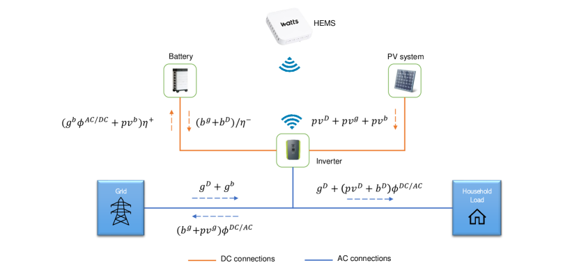
Figure 1: Schematic diagram of the home’s setup showing the AC and DC connections. The different average power flow terms, which are used in the mathematical representation of the system (Section 2.2), are also included.

The electricity generation from the PV system can be used to charge the home battery, to meet the EL demand, or can be exported to the grid. The electricity losses due to AC/DC and DC/AC conversions are included in the formulation. We assume that the electricity retailer communicates price information to the HEMS and that the HEMS has access to numerical weather predictions. Furthermore, NWPs are input to probabilistic load forecasting (PLF) models used for the creation of EL scenarios. The data of real consumers in Denmark is used, however, these consumers did not have PV installations. Thus, a simulation model for PV production is implemented and presented in Section 2.4. The remainder of this section introduces the mathematical model formulation for the above setup.

2.2 HEMS optimization model

The HEMS controller is formulated as a stochastic MILP [24], where the EL is the only uncertain parameter, i.e. having varying realizations across scenarios. The MILP in (1) minimizes the expected cost for fulfilling the EL in all scenarios $\mathcal{S}$ and periods $\mathcal{T}$. The main decision variables are the flows between the PV, grid, and battery components. The model considers several time periods due to the temporal interdependence imposed by the battery SoC in a rolling horizon manner. This means that, when applying the solution to the HEMS, only the optimal solution for the first time period is applied in practice. Decisions in subsequent periods are only considered to find optimal decisions for the first time step. This allows for re-optimization and taking relevant decisions with updated forecasts.

$$\min_{x_{s,t}^{\mathrm{-}},x_{s,t}^{\mathrm{+}}}\quad\sum_{s\in\mathcal{S}}\sum_{t\in\mathcal{T}}\pi_{s}(\lambda_{t}^{\mathrm{+}}x_{s,t}^{\mathrm{+}}-\lambda_{t}^{\mathrm{-}}x_{s,t}^{\mathrm{-}})$$ (1a)

subject to

$$D_{s,t}^{\mathrm{}}=(g_{s,t}^{\mathrm{D}}+(pv_{t}^{\mathrm{D}}+b_{s,t}^{\mathrm{D}})\phi^{\text{DC/AC}})\Delta t \forall\,t\in\mathcal{T},\,s\in\mathcal{S}$$ (1b)

$$x_{s,t}^{\mathrm{+}}=(g_{s,t}^{\mathrm{D}}+g_{s,t}^{\mathrm{b}})\Delta t \forall\,t\in\mathcal{T},\,s\in\mathcal{S}$$ (1c)

$$x_{s,t}^{\mathrm{-}}=(b_{s,t}^{\mathrm{g}}+pv_{t}^{\mathrm{g}})\phi^{\text{DC/AC}}\Delta t \forall\,t\in\mathcal{T},\,s\in\mathcal{S}$$ (1d)

$$x_{s,t}^{\mathrm{-}}\leq Mz_{s,t} \forall\,t\in\mathcal{T},\,s\in\mathcal{S}$$ (1e)

$$x_{s,t}^{\mathrm{+}}\leq M(1-z_{s,t}) \forall\,t\in\mathcal{T},\,s\in\mathcal{S}$$ (1f)

$$PV_{t}^{\mathrm{}}=(pv_{t}^{\mathrm{g}}+pv_{t}^{\mathrm{D}}+pv_{t}^{\mathrm{b}})\Delta t \forall\,t\in\mathcal{T}$$ (1g)

$$b_{s,t}^{\mathrm{+}}=(g_{s,t}^{\mathrm{b}}\phi^{\text{AC/DC}}+pv_{t}^{\mathrm{b}})\eta^{+} \forall\,t\in\mathcal{T},\,s\in\mathcal{S}$$ (1h)

$$b_{s,t}^{\mathrm{-}}=(b_{s,t}^{\mathrm{g}}+b_{s,t}^{\mathrm{D}})/\eta^{-} \forall\,t\in\mathcal{T},\,s\in\mathcal{S}$$ (1i)

$$b_{s,t}^{\mathrm{+}}\leq B^{\mathrm{in}} \forall\,t\in\mathcal{T},\,s\in\mathcal{S}$$ (1j)

$$b_{s,t}^{\mathrm{-}}\leq B^{\mathrm{out}} \forall\,t\in\mathcal{T},\,s\in\mathcal{S}$$ (1k)

$$b_{s,t}^{\mathrm{+}}\leq My_{s,t} \forall\,t\in\mathcal{T},\,s\in\mathcal{S}$$ (1l)

$$b_{s,t}^{\mathrm{-}}\leq M(1-y_{s,t}) \forall\,t\in\mathcal{T},\,s\in\mathcal{S}$$ (1m)

$$s_{s,t}^{\mathrm{}}=S^{\mathrm{ini}}+(b_{s,t}^{\mathrm{+}}-b_{s,t}^{\mathrm{-}})\Delta t \forall\,s\in\mathcal{S},\,t=1$$ (1n)

$$s_{s,t}^{\mathrm{}}=s_{s,t-1}^{\mathrm{}}+(b_{s,t}^{\mathrm{+}}-b_{s,t}^{\mathrm{-}})\Delta t \forall\,t\in\mathcal{T},\,s\in\mathcal{S},\,t>1$$ (1o)

$$S^{\mathrm{min}}\leq s_{s,t}^{\mathrm{}}\leq S^{\mathrm{max}} \forall\,t\in\mathcal{T},\,s\in\mathcal{S}$$ (1p)

$$b_{s,t}^{\mathrm{+}}=b_{j,t}^{\mathrm{+}}\,,\,b_{s,t}^{\mathrm{-}}=b_{j,t}^{\mathrm{-}} \forall s,j\in\mathcal{S},\,s\neq j,\,t=1$$ (1q)

$$s_{s,t}^{\mathrm{}}=s_{j,t}^{\mathrm{}} \forall s,j\in\mathcal{S},\,s\neq j,\,t=1$$ (1r)

The objective function (1a) minimizes the expected cost of electricity. Furthermore, constraint (1b) ensures that the consumer’s demand is satisfied in all scenarios. Electricity purchase and sale quantities are set in constraints (1c) and (1d). Constraints (1e) and (1f) ensure that electricity sale and purchase are mutually exclusive. The PV power balance is set in constraint (1g) such that the total generation meets the sum of PV production to grid, demand and battery. Constraints (1h), (1i), (1j), and (1k) model the physical battery behaviour in terms of power flow. Simultaneous charging and discharging of the battery is disallowed in constraints (1l) and (1m). The evolving SoC is modelled by constraints (1n) and (1o), while constraint (1p) limits the SoC to the battery capacity.

Since it is possible to re-optimize the solution after one time period, and the energy exchange with the grid is unrestricted, we can frame the problem as a two-stage stochastic problem. The first stage of the problem defines the operational schedules of the battery in the first period, as given by constraints (1q) and (1r). Thus, the battery charging and discharging in the first time period needs to be the same for all scenarios.

2.3 Electrical load forecast

The HEMS optimization model presented in Section 2.2 uses EL scenarios as input. The scenarios must consider the temporal correlation inherent to the EL. Thus, the multivariate PLF methods presented in [10] are used in this paper to generate the required scenarios. The methods use either Recursive Least Squares (RLS) with a full covariance model for the residuals or the quantile-copula with a full covariance model of the temporal correlation under the Gaussian domain and are referenced in [10] as RLS-Free and Copula-Free.

2.4 PV simulation

Another key element of the HEMS is the PV system. In this study, PV generation data were not available. Thus, a simulation approach is used to estimate a rooftop PV production. The simulation model is based on the guidelines provided in the energy data catalogue by the Danish Energy Agency [25]. The report suggests that electricity produced by a PV system should be estimated as

$$PV_{t}^{\mathrm{}}=PV^{peak}\cdot\frac{GHI_{t}}{1000}\cdot PV^{\mathrm{tf}}\cdot PV^{\mathrm{pr}}$$ (2)

where $PV^{peak}$corresponds to the PV production under laboratory standard test conditions (1000 $W/m^{2}$ irradiation with a cell temperature of 25°C), $PV^{tf}$ is the PV transposition factor and $PV^{pr}$ is the PV performance ratio. Moreover, the $GHI_{t}$ (global horizontal irradiation) values are calculated using the deterministic cloud cover to $GHI$ model described in [26] and given by

$$GHI_{t}=GHI_{t}^{CS}\cdot[0.35+0.65\cdot(1-CC)]$$ (3)

where $cc$ is the normalized cloud coverage (0 = clear, 1 = overcast) that is obtained from a NWP model, and the $GHI_{t}^{CS}$ is the clear sky $GHI$ that is estimated by the clear sky methods provided by the pvlib Python package [27].

3 Case study

In this section, we describe the input data used by the HEMS models presented in Section 2.1, and the technical details of the simulation setup used to calculate the results.

3.1 Electrical load

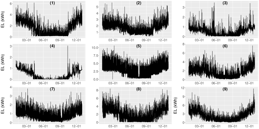
Figure 2: Consumers’ electricity consumption for the time period 2020-01-01 to 2020-12-31.

The EL demand profiles of nine residential consumers are shown in Figure 2. The consumption data results from smart meters sampled at an hourly resolution for the year 2020. Information given about these consumers includes the number of inhabitants, the approximate house location given by its longitude and latitude coordinates, and the fact that they use heat pumps as heating technology. The use of heat pumps explains the seasonality of the EL, i.e., a significantly higher consumption during winter in comparison to summer (see Figure 2). Although not visible in yearly plots, intra-day patterns can be found on a closer inspection of the data (see Figure 3). These patterns may be explained by the daily routine activities of the tenants, e.g., having breakfast and dinner at regular times. These factors together with the data presented in Section 3.2 were considered when building the PLF used for the scenario generation of each consumer load demand. While it is out of the scope of this paper to describe and analyze the PLF methods, they are described in detail in [10].

3.2 Numerical weather prediction

Both the PV simulation model (Section 2.4) and the PLF methods (Section 2.3) rely on the NWP values as their primary input parameters. Here, the weather forecast provided by the OpenWeatherMap service at an hourly resolution was used. The NWP data are described in [28]. In particular, the ambient temperature and solar irradiation were used for the PLF and PV models. Please note that the solar irradiation signal was derived using the expected cloud coverage from the NWPs in combination with the Global Horizontal Irradiation (GHI), as described in Section 2.4.

The EL and NWP data are combined to produce a coherent dataset used for the HEMS. An example week for one user is shown in Figure 3. Please note that the NWP is updated every hour with the forecast values covering several hours ahead ($k$ horizons). The NWP for one hour ahead $k=1$ and eighteen hours ahead $k=18$ are presented in Figure 3 (b) and (c).

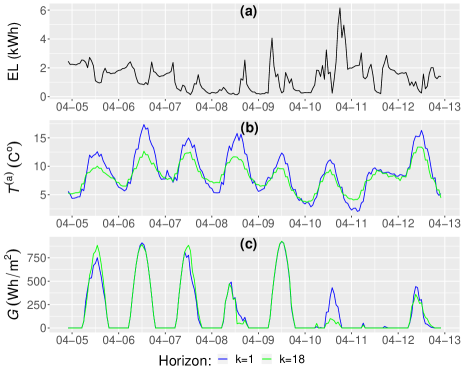
Figure 3: Consumer 1’s electricity consumption (a), ambient temperature (b), and solar irradiation (c) for the time period 2020-04-05 to 2020-04-13.

3.3 Electricity prices

Given the high penetration of smart meters in Denmark, it is common for electricity retailers to offer hourly prices to residential consumers. Typically, this type of tariff is derived from the day-ahead (DA) wholesale electricity market prices, also known as ELSPOT [29]. In the ELSPOT market, different zones/regions have their unique DA prices. In Denmark, two price zones zones exist: Western Denmark (DK1) and Eastern Denmark (DK2) [30]. To obtain the electricity prices for the residential consumers, retailers add taxes, levies, and fees to the DA prices. In this study, actual retail electricity prices provided by the Danish electricity retailer Watts are used [31]. All consumers are located in the greater Copenhagen area, which is a part of DK2 region. Figure 4 shows the retailer prices and DA electricity prices for the period of 2020-01-01 to 2021-12-03. The current Danish regulations allow residential consumers to sell their surplus electricity back to the grid. The feed-in-tariff is decided by the retailers. Most of them offer the ELSPOT price adjusted for associated operational fees as feed-in-tariff to residential consumers, as described by [32].

In our case study, Watts electricity prices are used as real-time price paid by the consumers to purchase electricity, while DA prices are used as feed-in-tariff for selling. This corresponds to the parameters $\lambda_{t}^{\mathrm{+}}$ and $\lambda_{t}^{\mathrm{-}}$, respectively (see Section 2.2).

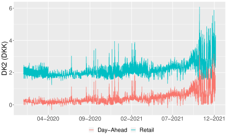
Figure 4: Retailer prices and DA electricity prices for the time period 2020-01-01 to 2021-12-03 for DK2.

Please note the differences in prices in 2020 and 2021. On the one hand, a tariff regulation change was introduced in 2021 that stipulates a low (between 00.00 to 17.00 and 20.00 to 00.00) and a peak (between 17.00 to 20.00) electricity distribution fee from October to March [33]. On the other hand, 2021 was a year with unusual electricity prices, i.e., high prices and high volatility [34], as can be seen in the final quarter of 2021 in Figure 4.

The HEMS setup and formulation allows cost reduction by selling excess electricity (excess electricity from PV), trading (buy at low-price hours to sell at high-price ones), and load shifting. This can be done by exploiting price volatility. Thus, for further reference, the mean and standard deviation of the prices are presented in Table 1. Note that the statistics are only presented for January, April, July, and October of 2021. These are the months that are included in the simulation setup described in Section 3.4. Please note that at present, consumers are mainly passive users of electricity, which has no significant effect on prices as they are price-takers [35].

Time	Purchase price		Selling price
Period	Mean	SD	Mean	SD
January 2020	1.943	0.164	0.206	0.074
January 2021	2.085	0.230	0.379	0.126
April 2020	1.797	0.107	0.129	0.086
April 2021	2.008	0.120	0.357	0.160
July 2020	1.858	0.144	0.191	0.115
July 2021	2.330	0.198	0.615	0.159
October 2020	1.921	0.193	0.202	0.118
October 2021	2.624	0.780	0.810	0.591

Table 1: Purchase and selling prices mean and standard deviation (SD) for January, April, July and October.

3.4 Simulation setup

The simulation study is designed to resemble a real-time application. The aim of the simulation is to optimize the battery’s operational setpoints for the next hour when considering a 24-hour horizon. Therefore, a rolling horizon approach is used, which means that the PLF, PV simulation, and HEMS optimization will be updated every hour to determine the new operation schedules. A graphical representation of the rolling horizon simulation setting at time $t$ is presented in Figure 5. Please note the PLF models are re-fitted using $t-N$ historical values at each time step $t$. Thus, more accurate prediction can be expected by using the latest available information from the forecasting models.

Figure 5: Graphical representation of the simulation setting for time $t$.

Four months of data (January, April, July and October) are selected as representative for seasonal variations in order to analyse one year of operation. Moreover, the prices used in the simulation are the prices in DK2 from 2021. This is motivated by the regulation changes introduced in that year. Please note that the consumers’ EL data were only available for 2020. Therefore, we used consumers’ data from 2020 with prices from 2021 in our simulations, assuming that the EL in the selected months of 2020 is likely to be similar to the EL in the same months in 2021 and the fact that residential consumers are price-takers.

4 Simulation results

In this section, we compare consumers’ cost savings when using different control strategies. Two such strategies are considered: a naive controller and an optimization-based controller. A naive controller refers to a consumer with PV and battery system without a HEMS. This controller maximizes self consumption by only selling electricity to the grid when the battery is fully charged. The naive controller uses neither forecasting nor optimization methods and it is usually the default controller in the HEMS setup presented in Section 2.1 [22]. The optimization-based controller refers to a consumer using a HEMS with optimization and forecast capabilities as presented in this paper. With this in mind, the rest of the results section is organized as follows. In Subsection 4.1, we determine the most suitable PLF method for the optimization-based controller by comparing the performance of the proposed HEMS optimization model using different forecasting methods. A comparison between the best optimization-based controller and a naive controller is presented in Subsection 4.2. Results indicate the optimal strategy is a combination of a naive and a optimal controller. This is presented in detail in Subsection 4.3.

4.1 Comparison of different optimization-based controllers

Con.	PI-RH		Copula-EV		Copula-SP		RLS-EV		RLS-SP
no.	DKK	%	DKK	%	DKK	%	DKK	%	DKK	%
1	5798.61	-	6220.66	7.28	5976.54	3.07	6143.84	5.95	5895.99	1.68
2	12142.80	-	12887.78	6.14	12553.15	3.38	12745.82	4.97	12438.41	2.43
3	6689.17	-	7259.67	8.53	6977.89	4.32	7398.95	10.61	6984.19	4.41
4	2071.31	-	2438.35	17.72	2210.56	6.72	2514.62	21.40	2183.16	5.40
5	1247.45	-	1638.04	31.31	1445.67	15.89	1695.82	35.94	1402.20	12.41
6	7435.47	-	8322.06	11.92	7887.49	6.08	8254.65	11.02	7824.03	5.23
7	9294.46	-	9945.68	7.01	9610.14	3.40	9903.44	6.55	9557.67	2.83
8	3157.25	-	3547.44	12.36	3312.33	4.91	3639.82	15.28	3316.83	5.05
9	6616.65	-	6970.68	5.35	6752.09	2.05	6954.68	5.11	6715.13	1.49

Table 2: Total cost of the optimization and forecasting methods. All percentages are calculated relative to the PI-RH method.

The PLF methods presented in [10] allow different combinations of forecasting and optimization methods. This section discusses the performance of such combinations in order to select the best method. The analyzed combinations are the following:

• RLS-SP: the proposed HEMS optimization using 100 scenarios generated by the RLS forecasting method.

• RLS-EV: the proposed HEMS optimization using the expected value of the 100 scenarios generated by the RLS forecasting method.

• Copula-SP: the proposed HEMS optimization using 100 scenarios generated by the Copula forecasting method.

• Copula-EV: the proposed HEMS optimization using the expected value of the 100 scenarios made by the Copula forecasting method.

• PI-RH: perfect information (PI) in a rolling horizon, i.e, using the proposed HEMS optimization assuming that the consumer’s load is known. This method is not applicable in practice, since the PI-RH method assumes a perfect knowledge of the future demand. But it can be used to give performance bounds on the optimization in the other settings.

Please note that “EV” methods correspond to a deterministic version of the HEMS stochastic model presented in Section 2.2. This allows us to assess the impact of modeling the EL uncertainty by comparing with “SP” methods. Table 2 presents the total electricity cost for the simulated months for the different combinations of forecasting and optimization methods. Moreover, the table reports the cost relative to the theoretical approach PI-RH expressed as percentages. The simulation results indicate that the optimization using scenarios-based stochastic programming outperforms the other solutions for all consumers, with the RLS-SP being the best method. It presents the smallest difference to the PI-RH. Considering that we re-optimize the solution after one time period, these results are aligned with the results in [10]. In [10], although the Copula-based forecast presented an overall better performance, the RLS-based forecast showed higher accuracy for the initial time period. This may indicate that the performance of the optimization depends to a high degree on the precision of the forecast in the initial time step.

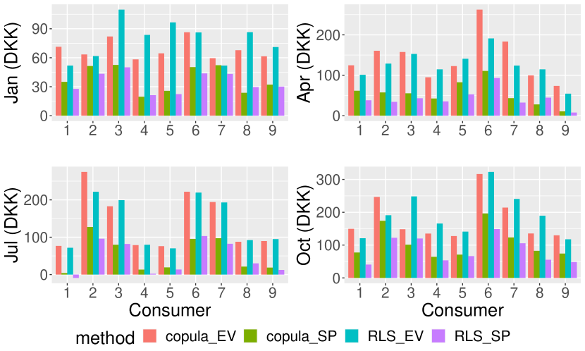
Figure 6: Additional cost by forecast and optimization framework in comparison with the PI-RH as baseline.

A cost comparison between the different methods on a monthly level is shown in Figure 6. The figure shows the additional cost incurred in each method in comparison to the PI-RH case as our baseline. Similar results as the aggregated results presented in Table 2 are seen, where the RLS-SP and Copula-SP methods outperform the deterministic methods in every season. Moreover, the simulation results indicate that in some cases, the solutions found through SP methods tend to be more robust than those determined assuming perfect information. This can be seen in the RLS-SP results for consumer 1 in July, where RLS-SP solutions outperform those of PI-RH. This may seem counterintuitive considering that PI-RH assumes perfect knowledge of uncertain EL, however, the PI is limited by the 24 hours in the rolling horizon. This behavior may indicate that considering the EL stochasticity may lead to more robust solutions towards the unpredicted EL and/or the optimization may benefit from a longer forecasting horizon.

4.2 Comparison of naive and optimal control

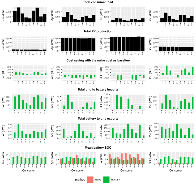
Figure 7: Monthly cost and operation results for the naive controller and RLS-SP.

In this section, we present the operational results for the optimization-based control method (RLS-SP) and the naive controller. Figure 7 shows the total load, total PV production, cost savings relative to the naive controller, total amount of electricity imported from the grid to the battery, the total power exported from the battery to the grid, and the average battery SOC for each consumer.

From the cost saving plots, we can observe significant differences between seasons. The RLS-SP outperforms the naive controller in winter (Jan) and autumn (Oct). In January, the additional cost savings can be explained by more load shifting. Here, the lower PV production available for self-consumption incentivizes more transactions with the grid, which can be seen by the higher grid-to-battery energy flow. Note that the battery-to-grid energy flow is non-significant. This indicates the optimization is taking advantage of the price volatility (see Table 1) by charging during low-price hours in order to use the stored electricity during high-price hours. October yields the highest cost savings of the simulated months. This is achieved by exploiting the high price volatility (the highest price volatility among the simulated months) in a similar fashion to January.

In contrast, spring (Apr) and summer (Jul) show the lowest cost savings. In these months, the RLS-SP controller is outperformed by the naive strategy. In particular, April presents a considerable EL with high PV production but low price volatility (see Table 1). This implies that the optimization minimizes cost by selling excess PV generation, which could be a sub-optimal strategy in the long-term given the gap between purchase and sale electricity prices (see Figure 4). In this case, the daily rolling optimization horizon might not be able to capture the longer-term effects and saving PV generation for posterior use will benefit the consumer the most. Furthermore, this argument matches the behavior seen in July, where the low EL, high PV production, and low price volatility leave almost no space for additional cost savings relative to the naive approach. Therefore, under these conditions, a naive approach is able to minimize consumers’ costs in the long-term, and the application of more sophisticated optimization-based methods could have a negative impact on cost minimization.

4.3 Combination of naive controller and optimization

As we have seen previously, the naive controller (which maximizes self consumption) performs better than the optimization-based methods in the presence of high PV production and low EL. This behavior could be explained as a result of the price structure and volatility, and the implications of the finite optimization horizon. The optimization minimizes short-term cost by selling excess electricity, since it plans no more than 24 hours ahead. However, sale prices are very unfavorable in comparison with purchase prices, which makes self-consumption a better long-term strategy. Thus, one option could be to have a HEMS switching between a naive controller in the spring and summer and to use an optimization-based control strategy in the autumn and winter seasons. Hence, a full cost comparison between a passive consumer (without PV and battery), a naive controller, and the proposed strategy (Naive+RLS-SP) is presented in Table 3. The results show that significant cost savings can be achieved in the naive and the proposed strategy in comparison with a passive consumer. In particular, the simulation results show that consumers with higher EL benefit most from installing the hardware and controllers. Moreover, the differences between the two control strategies show that the combined controller (Naive+RLS-SP) provides on average 8.05% additional savings for consumers with higher load (excluding consumers 4 and 5 with the lowest load of all consumers) in comparison with the naive controller, as can be seen in detail in Table 4.

Consumer	Passive		Naive		Naive+RLS-SP
no.	DKK	%	DKK	%	DKK	%
1	9219.20	-	6015.12	34.75	5825.17	36.81
2	16734.67	-	12715.96	24.01	12248.38	26.81
3	10799.02	-	6972.54	35.43	6735.15	37.63
4	5353.58	-	2140.78	60.01	2094.73	60.87
5	3901.01	-	1281.02	67.16	1332.69	65.84
6	11208.06	-	7827.33	30.16	7544.91	32.68
7	13370.53	-	9695.89	27.48	9333.01	30.20
8	6455.34	-	3331.51	48.39	3184.64	50.67
9	10806.51	-	6935.86	35.82	6563.42	39.26

Table 3: Total cost of the simulated months for passive consumers, and naive and optimal (naive+RLS-SP) control strategies. All percentage values are calculated relative to the passive consumers’ cost.

Consumer No.	Naive	Naive+RLS-SP	Difference	%
1	3204.09	3394.03	189.95	5.93
2	4018.70	4486.29	467.59	11.64
3	3826.48	4063.87	237.39	6.20
4	3212.80	3258.85	46.05	1.43
5	2619.99	2568.32	-51.67	-1.97
6	3380.73	3663.15	282.42	8.35
7	3674.64	4037.51	362.87	9.88
8	3123.83	3270.70	146.88	4.70
9	3870.65	4243.09	372.44	9.62

Table 4: Naive and optimal control strategies (naive+RLS-SP) total cost savings and their difference in value and percentage.

5 Discussion

The simulation results from Section 4.1 show that EL uncertainty has a significant impact on the economic performance of the optimization-based strategies, with the stochastic methods outperforming the deterministic methods. While it appears clear that including EL uncertainty increases the consumers’ economic benefits, the lack of access to real PV data limits the ability to study the impact of modeling the uncertainty inherent to the PV generation on the system operation. To consider the PV uncertainty, one needs to account for the correlation between the PV and EL time series, which could be technically challenging in a multivariate setting. This could be a topic for future research.

A comparison between naive and optimal control strategies, presented in Section 4.2, shows that the seasonal variations and the electricity price structure have a significant impact on the performance of the control strategies. During cold seasons with low PV production and higher EL, an optimization-based strategy is preferable in order to exploit price volatility by load shifting, charging the battery at low-price hours and discharging it during high-price hours. In warmer seasons with low price volatility, lower EL and PV make the naive strategy a better option. This could be explained by the fact that under these conditions, a long-term self-consumption strategy might be more profitable, which the optimization-based controller fails to capture due to its finite optimization horizon. Please note that this dynamic is tied to the price structure, where high differences between purchase and sale prices do not incentivize consumers to trade electricity. This may have a direct impact on the consumers in studies where market entities such as aggregators are present. Under current market conditions, aggregators will have to offer prices that surpass the retail prices. Otherwise, the consumers will not participate in the aggregation programs. Thus, studying different business models for aggregators under realistic price structures could be a line of future research.

The simulation results presented in Section 4.3 indicate that the overall best control among the studied strategies is a combination of a naive and optimization-based controllers. This is shown by the proposed Naive+RLS strategy that outperforms the naive controller by 8.05% on average (excluding users 4 and 5). Please note that these extra savings result from a software update on the default system controller, which does not incur additional cost to the consumers. Additionally, the results obtained for customers 4 and 5 suggest a self-consumption strategy benefits the consumer the most when the EL is low, making more elaborated control strategies unnecessary in practice.

As smart grids continue to develop and price schemes evolve into a real-time structure, the proposed setup and control strategy shows that there is an incentive for consumers to adopt setups such as the one presented in this paper. Moreover, if we consider that a higher energy demand and a higher penetration of RES is expected in the residential sector, we could argue that these types of automation system might become a much needed tool for consumers to protect themselves against higher price volatility. Furthermore, although the proposed HEMS omits elements such as direct control of smart appliances and electric vehicles, we would expect their inclusion to bring higher savings for the consumer, which is a further element that could be explored in future research. While the economic results presented here show potential economical advantages of HEMS, the calculations were made for 2021 only. Future scenarios of electricity prices could be included and analyzed in future research in this area.

6 Conclusion

In this paper, a HEMS setup tailored for residential consumers under current electricity market rules in Denmark was presented. The HEMS was formulated as a MILP using stochastic programming, where the EL is treated as an uncertain parameter, which is modelled by multivariate probabilistic forecast models. Moreover, the HEMS formulation allows selling surplus electricity back to the grid depending on the price incentives and the re-optimization of the solution in a rolling horizon fashion.

The simulation results suggest that the optimization-based controllers, which consider the EL uncertainty, outperform their counterparts that consider only the expected value of the EL for all users and seasons investigated. Specifically, by comparing the RLS-SP controller with the naive one, we found that the seasonality of the data and prices have a profound impact on the cost-savings of all users. One possible explanation could be that the finite optimization horizon and the gap between purchase and sale prices lead to sub-optimal solutions of the optimization-based controller in spring and summer, which are seasons with high PV production and low EL. In these seasons, a naive controller performs better. On the other hand, in autumn and winter with low PV production and high EL, optimization-based controllers exploit price volatility by shifting load to minimize electricity cost. Thus, the proposed combination of a naive and optimization-based strategy was shown to reduce the annual consumers’ electricity cost in comparison with the naive method as a year-around controller. These savings are specifically significant considering that the proposed change of strategies in different seasons may come as a software update with small cost for the consumers. Finally, the case study showed that the proposed setup and control strategy offer a significant step towards a comprehensive assessment of the potential of HEMSs, indicating that the setup and control strategy could be developed in real-world applications of HEMSs.

References

- [1] European parliament. Directive 2012/27/EU of the European Parliament and of the Council of 25 October 2012 on energy efficiency, amending Directives 2009/125/EC and 2010/30/EU and repealing Directives 2004/8/EC and 2006/32/EC. https://eur-lex.europa.eu/legal-content/EN/TXT/?uri=CELEX%3A02012L0027-20210101, accessed on 2022-01-22.
- [2] Energinet. Rates — Energinet. https://energinet.dk/El/Elmarkedet/Tariffer, accessed on 2022-01-22.
- [3] D. Mariano-Hernández, L. Hernández-Callejo, A. Zorita-Lamadrid, O. Duque-Pérez, and F. Santos García. A review of strategies for building energy management system: Model predictive control, demand side management, optimization, and fault detect & diagnosis. Journal of Building Engineering, 33:101692, jan 2021.
- [4] Murray Goulden, Ben Bedwell, Stefan Rennick-Egglestone, Tom Rodden, and Alexa Spence. Smart grids, smart users? The role of the user in demand side management. Energy Research & Social Science, 2:21–29, jun 2014.
- [5] Lena Hansson, Ulrika Holmberg, and Helene Brembeck. Making sense of consumption : selections from the 2nd Nordic Conference on Consumer Research 2012. In 2nd Nordic Conference on Consumer Research, page 393, 2012.
- [6] R. Balakrishnan and V. Geetha. Review on home energy management system. Materials Today: Proceedings, 47:144–150, jan 2021.
- [7] Claire McIlvennie, Angela Sanguinetti, and Marco Pritoni. Of impacts, agents, and functions: An interdisciplinary meta-review of smart home energy management systems research. Energy Research & Social Science, 68:101555, oct 2020.
- [8] Mojtaba Yousefi, Amin Hajizadeh, Mohsen N. Soltani, Branislav Hredzak, and Nasrin Kianpoor. Profit assessment of home energy management system for buildings with A-G energy labels. Applied Energy, 277:115618, nov 2020.
- [9] Marcelo Salgado, Matias Negrete-Pincetic, Álvaro Lorca, and Daniel Olivares. A low-complexity decision model for home energy management systems. Applied Energy, 294:116985, jul 2021.
- [10] Julian Lemos-Vinasco, Peder Bacher, and Jan Kloppenborg Møller. Probabilistic load forecasting considering temporal correlation: Online models for the prediction of households’ electrical load. Applied Energy, 303:117594, dec 2021.
- [11] Seyyed Reza Ebrahimi, Morteza Rahimiyan, Mohsen Assili, and Amin Hajizadeh. Home energy management under correlated uncertainties: A statistical analysis through Copula. Applied Energy, 305:117753, jan 2022.
- [12] Miadreza Shafie-Khah and Pierluigi Siano. A stochastic home energy management system considering satisfaction cost and response fatigue. IEEE Transactions on Industrial Informatics, 14(2):629–638, 2018.
- [13] Saeed Zeynali, Naghi Rostami, Ali Ahmadian, and Ali Elkamel. Two-stage stochastic home energy management strategy considering electric vehicle and battery energy storage system: An ANN-based scenario generation methodology. Sustainable Energy Technologies and Assessments, 39:100722, jun 2020.
- [14] Carlos Adrian Correa-Florez, Alexis Gerossier, Andrea Michiorri, and Georges Kariniotakis. Stochastic operation of home energy management systems including battery cycling. Applied Energy, 225:1205–1218, sep 2018.
- [15] Nikolaos G. Paterakis, Iliana N. Pappi, João P.S. Catalão, and Ozan Erdinc. Optimal operation of smart houses by a real-time rolling horizon algorithm. IEEE Power and Energy Society General Meeting, 2016-Novem, nov 2016.
- [16] Mahmoud Elkazaz, Mark Sumner, Richard Davies, Seksak Pholboon, and David Thomas. Optimization based Real-Time Home Energy Management in the Presence of Renewable Energy and Battery Energy Storage. SEST 2019 - 2nd International Conference on Smart Energy Systems and Technologies, sep 2019.
- [17] Tom Hargreaves, Charlie Wilson, and Richard Hauxwell-Baldwin. Learning to live in a smart home. https://doi.org/10.1080/09613218.2017.1286882, 46(1):127–139, jan 2017.
- [18] Larissa Nicholls, Yolande Strengers, and Sergio Tirado. Smart home control: Exploring the potential for off-the-shelf enabling technologies in energy vulnerable and other households. Energy Consumers Australia, 2017.
- [19] Larissa Nicholls and Yolande Strengers. Peak demand and the ‘family peak’ period in Australia: Understanding practice (in)flexibility in households with children. Energy Research & Social Science, 9:116–124, sep 2015.
- [20] Sergio Tirado Herrero, Larissa Nicholls, and Yolande Strengers. Smart home technologies in everyday life: do they address key energy challenges in households? Current Opinion in Environmental Sustainability, 31:65–70, apr 2018.
- [21] Nord pool group. Rules and regulations. https://www.nordpoolgroup.com/trading/Rules-and-regulations/, accessed on 2022-01-26.
- [22] Donald Azuatalam, Kaveh Paridari, Yiju Ma, Markus Förstl, Archie C. Chapman, and Gregor Verbič. Energy management of small-scale PV-battery systems: A systematic review considering practical implementation, computational requirements, quality of input data and battery degradation. Renewable and Sustainable Energy Reviews, 112:555–570, sep 2019.
- [23] L, Sevdari, and K. Marinelli. Status e-mobility DK. Technical report, Technical University of Denmark (DTU), 2021. https://orbit.dtu.dk/en/publications/status-e-mobility-dk.
- [24] John R. Birge and François Louveaux. Introduction to Stochastic Programming. Springer Series in Operations Research and Financial Engineering. Springer New York, New York, NY, 2011.
- [25] Danish Energy Agency. Technology Data for Generation of Electricity and District Heating — Energistyrelsen.
- [26] David P. Larson, Lukas Nonnenmacher, and Carlos F.M. Coimbra. Day-ahead forecasting of solar power output from photovoltaic plants in the American Southwest. Renewable Energy, 91:11–20, jun 2016.
- [27] William F. Holmgren, Clifford W. Hansen, and Mark A. Mikofski. pvlib python: a python package for modeling solar energy systems. Journal of Open Source Software, 3(29):884, sep 2018.
- [28] OpenWeather Ltd. Point forecast description. https://openweathermap.org/api/hourly-forecast, accessed on 2020-08-26.
- [29] Nord pool group. Day-ahead market. https://www.nordpoolgroup.com/the-power-market/Day-ahead-market/, accessed on 2021-11-01.
- [30] Nord pool group. Bidding areas. https://www.nordpoolgroup.com/the-power-market/Bidding-areas/, accessed on 2022-02-01.
- [31] Watts A/S. How much is a kWh? https://watts.dk/en/elprodukt/hvad-koster-en-kwh/, accessed on 2021-11-02.
- [32] Vindstød. Billig el fra danske vindmøller — Vindstød. https://www.vindstoed.dk/solcelle, accessed on 2021-11-10.
- [33] Radius A/S. Tariffer og netabonnement - få et overblik her på siden. https://radiuselnet.dk/elkunder/priser-og-vilkaar/tariffer-og-netabonnement/, accessed on 2021-12-23.
- [34] European commission. EU Energy prices. https://energy.ec.europa.eu/topics/markets-and-consumers/eu-energy-prices_en, accessed on 2022-01-22.
- [35] Anne Immonen, Jussi Kiljander, and Matti Aro. Consumer viewpoint on a new kind of energy market. Electric Power Systems Research, 180:106153, mar 2020.