Gas phase metallicity determinations in nearby AGNs with SDSS-IV MaNGA: evidence of metal poor accretion

Abstract

We derive the metallicity (traced by the O/H abundance) of the Narrow Line Region ( NLR) of 108 Seyfert galaxies as well as radial metallicity gradients along their galaxy disks and of these of a matched control sample of no active galaxies. In view of that, observational data from the SDSS-IV MaNGA survey and strong emission-line calibrations taken from the literature were considered. The metallicity obtained for the NLRs was compared to the value derived from the extrapolation of the radial oxygen abundance gradient, obtained from H ii region estimates along the galaxy disk, to the central part of the host galaxies. We find that, for most of the objects ($\sim 80\,\%$), the NLR metallicity is lower than the extrapolated value, with the average difference ($<D>$) between these estimates ranging from 0.16 to 0.30 dex. We suggest that $<D>$ is due to the accretion of metal-poor gas to the AGN that feeds the nuclear supermassive black hole (SMBH), which is drawn from a reservoir molecular and/or neutral hydrogen around the SMBH. Additionally, we look for correlations between $D$ and the electron density ($N_{\rm e}$), [O iii]$\lambda$5007 and H$\alpha$ luminosities, extinction coefficient ($A_{V})$ of the NLRs, as well as the stellar mass ($M_{*}$) of the host galaxies. Evidences of an inverse correlation between the $D$ and the parameters $N_{\rm e}$, $M_{*}$ and $A_{\rm v}$ were found.

1 Introduction

Emission line intensities present in the optical spectra of Active Galactic Nuclei (AGNs) and star forming regions (SFs) are essential to estimate the physical properties of the gas phase, such as metallicity, chemical abundances of heavy elements (e.g. O, N, S), electron temperature, and electron density of these objects. In particular, due to their high luminosity and prominent emission lines, AGNs play a key role in studies of the chemical evolution of galaxies along the Hubble time.

Oxygen abundance is usually used to estimate gas-phase metallicity of SFs (e.g. Kennicutt et al. 2003; Hagele et al. 2008; Yates et al. 2012) and of AGNs (e.g. Storchi-Bergmann et al. 1998; Dors et al. 2015, 2020a; Revalski et al. 2018; Flury & Moran 2020; Dors 2021). This is due to the oxygen is the third most abundant element after hydrogen and helium and it presents prominent optical emission lines ([O ii]$\lambda$3726,$\lambda$3729, [O iii]$\lambda$5007) of its most abundant ions ($\rm O^{+}$, $\rm O^{2+}$) measured in most part of the spectra with high signal noise ratio. In fact, Skillman & Kennicutt (1993) and Dors et al. (2020a) found that the ion abundances with ionization stage higher $\rm O^{2+}$ do not exceed $\sim 5\,\%$ and $\sim 20\,\%$ of the total O/H abundance in SFs and AGNs, respectively. Therefore, such as in Krabbe et al. (2021), hereafter we use metallicity ($Z$) and oxygen abundance [in units of 12 + log(O/H)] interchangeably.

The metallicity has been estimated preferably by comparisons between observational emission line ratios (e.g. [O ii]($\lambda$3726+$\lambda$3729)/H$\beta$, [O iii]$\lambda$5007/H$\beta$, [N ii]$\lambda$6584/H$\alpha$) with those predicted by photoionization models. One of the first $Z$ determinations in AGNs was carried out by Ferland & Netzer (1983), who compared observed and model predicted optical emission line ratios of low ionization nuclear emission-line regions (LINERs) and Seyferts using the Cloudy code (for the updated version see Ferland et al., 2017). These authors found that the observed emission-line ratios were well reproduced by photoionization models with metallicity in the range $0.1\>\la\>(Z/{\rm Z_{\odot}})\>\la 1.0$. After this pioneering work, several studies have been performed with the goal to estimate $Z$ in AGNs located at low (e.g. Stasińska 1984; Ferland & Osterbrock 1986; Storchi-Bergmann et al. 1998; Groves, Heckman & Kauffman 2006; Feltre, Charlot & Gutkin 2016; Castro et al. 2017; Pérez-Montero et al. 2019; Carvalho et al. 2020) and high redshifts (e.g. Nagao, Maiolino & Marconi et al. 2006; Matsuoka et al. 2009, 2018; Nakajima et al. 2018; Dors et al. 2018, 2019; Mignoli et al. 2019; Guo et al. 2020; Ji et al. 2020) by using photoionization models. Particularly, Storchi-Bergmann et al. (1998) proposed the first theoretical calibrations between strong optical emission-line ratios and metallicity, thus allowing estimations of $Z$ in large samples of AGNs and the development of new calibrations (e.g. Dors et al. 2014, 2019; Castro et al. 2017; Carvalho et al. 2020; Dors 2021). Storchi-Bergmann et al. (1998) found that the $Z$ values of seven Seyfert 2 nuclei, derived from their calibrations, are in agreement (within an uncertainty of $\sim$0.2 dex) with those inferred from extrapolation of the oxygen abundance gradient to central parts of the hosting spiral galaxy. Thereafter, Dors et al. (2015) performed similar analysis but for a larger sample of AGNs (12 Seyfert 2) and star-forming nuclei (33 objects). Dors et al. (2015) found that direct central oxygen abundances (i.e. estimates based on emission-line ratios from the nuclei) in some high-metallicity galaxies tend to be lower than the extrapolated abundances.

The existence of lower oxygen abundances in the narrow line region of AGNs compared to the extrapolated value of abundance gradients is very important in chemical evolution studies of galaxies, since it indicates that the nuclear region could have distinct chemical evolution as compared to the disk. This discrepancy can be due to the following physical processes:

• Spiral galaxies in the local universe can be accreting metal-poor gas from the outskirts of the disk onto the centres, a process more common at very high redshift (e.g. Cresci et al. 2015; Gillman et al. 2021). However, cases at low redhift have also been reported in dwarf galaxies, e.g. in NGC 2915 (Werk et al., 2010) and in NGC 4449 (Kumari, James, & Irwin, 2017).

• The gas phase of AGNs can have a distinct depletion of oxygen onto dust grains (e.g. Sternberg et al. 1994; Usero et al. 2004) in comparison to the one in disk H ii regions (of the order of 0.1 dex, e.g. Esteban et al. 1998; Meyer et al. 1998; Izotov et al. 2006; Jenkins 2009; Whittet 2010).

• There is metal-poor inflow of gas that can be originated from the capture of low mass companions to the nuclear region that ends up feeding the supermassive black hole (e.g. Storchi-Bergmann et al. 2007).

To investigate which of these processes are acting in AGNs it is necessary to estimate the metallicity in the entire galaxy, i.e. to consider estimates along the disk and in the nuclear region. Sánchez et al. (2014), by using observational data of galaxies ($0.003\>\la\>z\>\>\la 0.02$) selected by the Calar Alto Legacy Integral Field Area (CALIFA) survey (Sánchez et al., 2012), derived the oxygen gradients in about 300 spiral galaxies. However, the analysis carried out by Sánchez et al. (2014) was mainly based on galaxies containing star-forming nuclei. Another example is the CHAOS survey (Berg et al. 2015; Croxall et al. 2015, 2016; Berg et al. 2020; Skillman et al. 2020; Rogers et al. 2021), which has the selection criterion to observe only galaxies with star-forming nuclei. However, surveys such as Sydney Australian Astronomical Observatory Multi-object Integral Field Spectrograph (SAMI, Croom et al. 2012), although not dedicated to chemical evolution studies has provided valuable information on the nature of AGNs and their host galaxies (e.g. Comerford & Greene 2014; Allen et al. 2015; Hampton et al. 2017).

In this work, we used data from the Mapping Nearby Galaxies at Apache Point Observatory (MaNGA) survey (Bundy et al., 2015). We were motivated to consider these data due to the existence of previous galaxy selections by Rembold et al. (2017), which included a large sample of objects with confirmed AGNs and their control sample containing non-active galaxies. This advantage provides an excellent opportunity to compare the direct AGN estimates with those obtained from oxygen extrapolation gradients, as they cover larger parts of the disk in galaxies, including the nuclear region. Additionally, it is useful to compare metallicity estimates in AGNs hosts sample with a sample of control galaxies, in order to verify if there is any different effect on the metallicity gradient between them. This paper is organized as follows: In Section 2, a brief description of the sample of objects is presented as well as the methods used for estimating the oxygen abundance of the AGNs and the oxygen abundance gradients of the sample. In Sect. 3, we present the results and discussion. In Sect. 4, the summary and the conclusions are presented.

2 Methodology

We selected from the MaNGA database (Bundy et al., 2015) a sample of spiral galaxies hosting AGNs. The emission-line intensities of the AGN and strong-line calibrations proposed in the literature were used to estimate the oxygen abundances of these objects. In addition, emission-line intensities of star-forming regions located along the disk were used to calculate the oxygen abundance gradient in each galaxy of the sample, and calibrations available in the literature were also considered. In the subsequent sections a description of the methodology adopted to obtain the observational data and the abundance values are presented.

2.1 Observational data

The sample of galaxies studied here comprise both galaxies hosting AGNs as well as a sample of control galaxies selected as in Rembold et al. (2017). For each AGN was chosen two control non-active galaxies matching the AGN host stellar mass, morphology, distance and inclination. After the release of the MaNGA Product Launch 8 (MPL-8, Aguado et al., 2019; Blanton et al., 2017; Wake et al., 2017; Law et al., 2015, 2016; Yan et al., 2016; Drory et al., 2015; Gunn et al., 2006; Smee et al., 2013), the number of observed AGNs with MaNGA has grown to 170 AGNs and 291 control galaxies as described in Riffel et al. (2021). We classified the nuclei (central region with 2.5 arcsec diameter) and the regions along the disk of the galaxies according to their emission-line ratios in the diagnostic diagram [O iii]$\lambda$5007/H$\alpha$ versus [N ii]$\lambda$6584/H$\alpha$, proposed by Baldwin, Phillips & Terlevich (1981) (hereafter called BPT diagram) and on the WHAN diagram proposed by Cid Fernandes et al. (2010).

Firstly, to classify the regions in the sample as AGN-like and H ii-like objects, we used the theoretical and the empirical criteria proposed by Kewley et al. (2001) and Kauffmann et al. (2003), respectively. These criteria establish that regions with:

$$\rm log([O\>III]\lambda 5007/H\beta)\>>\>\frac{0.61}{log([N\>II]\lambda 6584/H\alpha)-0.47}+1.19$$ (1)

and

$$\rm log([O\>III]\lambda 5007/H\beta)\><\>\frac{0.61}{log([N\>II]\lambda 6584/H\alpha)-0.05}+1.3$$ (2)

are classified as AGN-like objects, otherwise, as H ii-like objects. Additionally, we applied the criterion proposed by Cid Fernandes et al. (2010) to separate AGN-like and Low-ionization nuclear emission-line region (LINER) objects, given by

$$\rm log([O\>III]\lambda 5007/H\beta)\>>\>0.47+log([N\>II]\lambda 6584/H\alpha)\times 1.01,$$ (3)

where the values satisfying the above criterion correspond to Seyferts, otherwise, they are classified as LINERs. Secondly, for each spaxel of the objects of our sample, the WHAN diagram proposed by Cid Fernandes et al. (2010), which takes into account the equivalent width of H$\alpha$ versus the [N ii]$\lambda$6584/H$\alpha$ line ratio, was considered to classify AGN-like and H ii-like objects. This same procedure has been previously illustrated and applied in do Nascimento et al. (2019).

After applying the aforementioned classification criteria, we selected the Seyfert type galaxies for our analysis using the final sample which consist of 98 Seyfert 2 and 10 Seyfert 1 galaxies as well as their respective control galaxies (145 in the total) for the present study. Among the 108 Seyfert galaxies, 71 are also classified as Seyfert using Sloan Digital Sky Survey (SDSS, York et al. 2000) III/Baryonic Oscillation Spectroscopic Survey (BOSS) collaboration data and flux measurements from Thomas et al. (2013) – the procedure originally used to identify the AGNs in the first paper of our series (Rembold et al., 2017). The remaining 26 are classified as LINERs on the basis of SDSS-III data. The larger number of Seyfert nuclei identified in the MaNGA data than those obtained using the 3.0 arcsec diameter SDSS-III fiber measurements, which is likely due to the better angular resolution of MaNGA. As gas surrounding the Seyfert region frequently shows LINER excitation (e.g. do Nascimento et al., 2019), the larger aperture of the SDSS-III data should be including more of the surrounding LINER region, as well as the possible contribution of emission from gas ionized by extra-nuclear evolved stars, moving the borderline objects from the Seyfert region to the LINER region of the BPT diagram. The radial oxygen gradient in each object covers a region measured in effective radii ($R_{\rm e}$) ranging from $\sim$0.5 to $\sim$2.5 (see also Mingozzi et al. 2020).

The median point spread function (PSF) of the MaNGA datacubes is estimated to have a full width at half maximum (FHWM) of about 2.5 arcsec (Law et al., 2015), which can be considered the resolution element in the data. The redshift values of our sample are in the range $0.02\la z\la 0.08$. Assuming a spatially flat cosmology with $H_{0}$ = 71 $\rm km\>s^{-1}Mpc^{-1}$, $\Omega_{m}=0.270$, and $\Omega_{\rm vac}=0.730$ (Wright, 2006), each resolution element represents a region with diameters in the range $\sim$1-4 kpc at the distance of the MaNGA sample. Thus, since H ii regions have typical sizes of tens to a few hundreds parsecs, each resolution element spectrum comprises the flux of a complex of H ii regions (Belfiore et al., 2017), and the physical properties derived represent an average value of these regions (e.g. Hagele et al. 2008; Krabbe et al. 2014; Rosa et al. 2014). However, this fact has little influence on the radial oxygen abundance in spiral galaxies because it is expected that H ii regions located at similar galactocentric distances present about the same metallicity (e.g. Kennicutt et al. 2003) and similar stellar content (e.g. Dors et al. 2017; Zinchenko et al. 2019).

Following Ilha et al. (2019), the emission-line fluxes from the MaNGA data cube were obtained by fitting a single-Gaussian component using the Gas AND Absorption Line Fitting (GANDALF; Sarzi et al., 2006) routine. The choice of this routine was due to the fact that it fits both the stellar population spectra and the profiles of the emission lines, after the subtraction of the stellar population contribution. A detailed description of the fitting procedure is presented in Ilha et al. (2019).

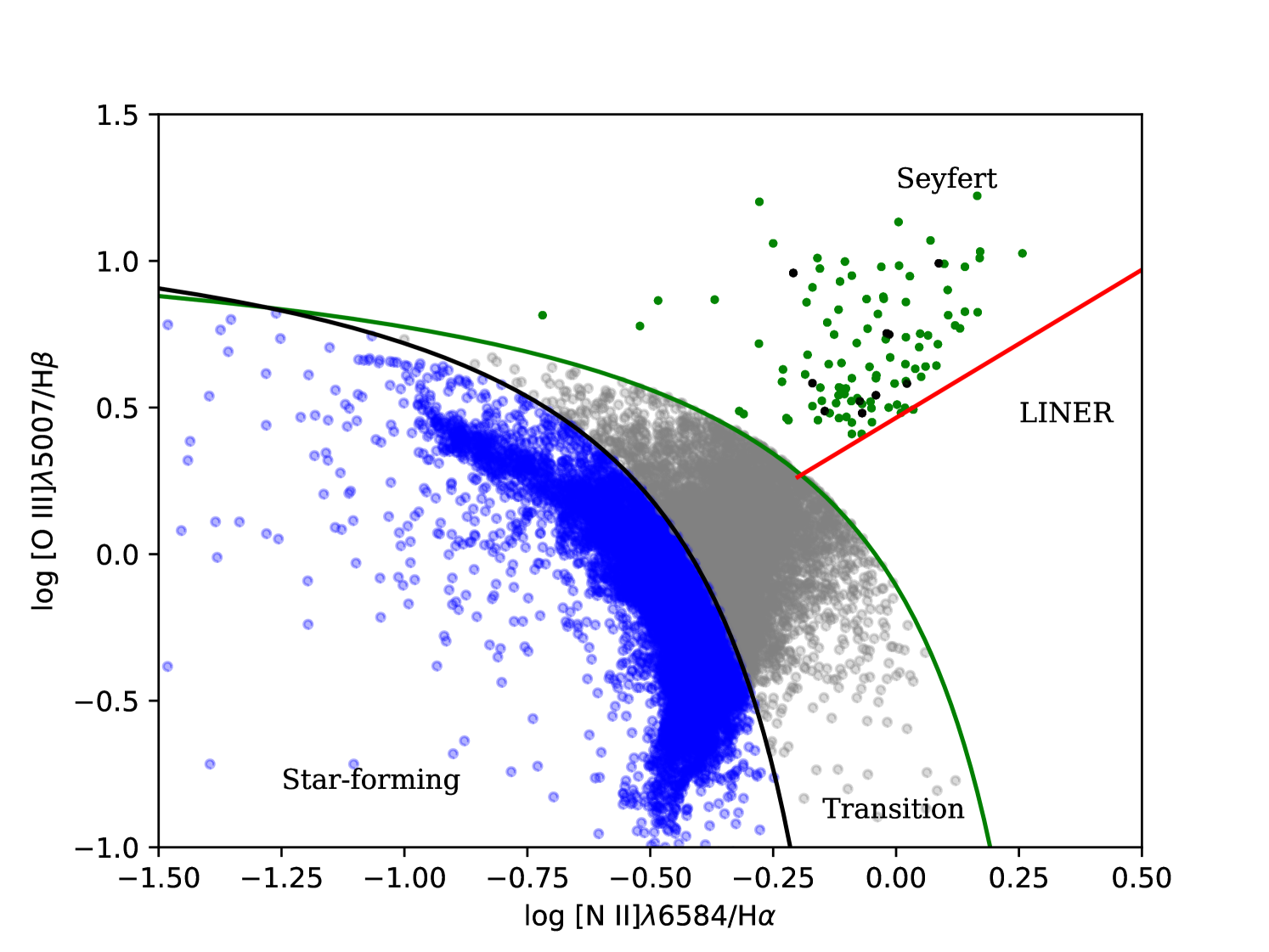
Figure 1: [O iii]$\lambda$5007/H$\beta$ versus [N ii]$\lambda$6584/H$\alpha$ diagnostic diagram for the AGN sample. The green (Seyfert 2) and the black points (Seyfert 1) correspond to the emission-line ratios of the AGNs, obtained by summing the fluxes of all spaxels within an aperture of 2.5 arcsec in diameter in the central region of each galaxy. The blue and gray points are star-forming and transition regions, respectively, whose emission-line ratios were obtained from each spaxel of the datacubes. Black and green lines correspond to the empirical and theoretical criteria to separate AGN-like and H ii-like objects proposed by Kauffmann et al. (2003) and Kewley et al. (2001), i.e. Eqs. 1 and 2, respectively. Red line represents the criterion proposed by Cid Fernandes et al. (2010) to separate AGN-like and LINERs (Eq. 3).

In Figure 1 we present the BPT diagram for the central region of the AGN and all other spaxels for the AGN and control sample that correspond to H ii and transition regions. The red line – marking the separation between Seyfert and LINER excitation was obtained from Kewley et al. (2006); the green line – marking the separation between the transition and AGN regions was obtained from Kewley et al. (2001) and the black line – marking the separation between the starburst and transition regions, was obtained from Kauffmann et al. (2003). Black circles and green triangles correspond to the emission-line ratios for the AGNs, obtained by summing the fluxes of all spaxels within a central aperture of 2.5 arcsec diameter. The Seyfert 2 galaxies are represented by the black circles and Seyfert 1 by the green triangles. Blue points are star-forming regions and grey points are transition regions. The diameter of the AGN nucleus of the galaxies is based on a fixed angular diameter of 2.5 arcsec and it ranges from $\sim$1 to $\sim$6 kpc according to the distance of each object. Thus, for some AGNs, an extended emission is observed.

2.2 Gas-phase metallicity determinations

We estimated the gas phase metallicity in relation to the solar value ($Z/\rm Z_{\odot})$ for each AGN and the oxygen radial gradients along the disk of each galaxy of the sample.

In the AGN and in the disk H ii region spectra of our sample emission lines sensitive to the electron temperature (e.g. [O iii]$\lambda$4363, [N ii]$\lambda$5755) were not detected and, consequently, it was not possible to calculate the elemental abundances by using the $T_{\rm e}$-method. Therefore, the O/H abundance or the metallicity was calculated through calibrations based on strong emission-lines. Several authors have investigated the O/H discrepancy values obtained when distinct methods are assumed and differences up to 0.6 dex have been found for H ii regions (e.g. Kewley & Ellison 2008; Lòpez-Sanchez et al. 2012; Peña-Guerrero et al. 2012). About the same discrepancy (i.e. up to 0.8 dex) is also derived for metallicity AGN estimates taking into account different methods, being the highest discrepancy values derived for the low-metallicity regime ($\rm 12+\log(O/H)\>\la\>8.5$, Dors et al. 2020b).

For H ii regions, there seems to be a consensus that reliable calibrations are those that produce O/H values similar (or near) to values derived through the $T_{\rm e}$-method (see Peimbert et al. 2017; Pérez-Montero 2017 for a review). For AGNs, it is available in the literature theoretical (Storchi-Bergmann et al., 1998), semi-empirical (Castro et al., 2017; Carvalho et al., 2020; Dors et al., 2021) and empirical (Dors, 2021) calibrations between strong optical narrow emission-lines and the metallicity or abundances. The recent empirical calibration for AGNs proposed by Dors (2021) requires measurements of the [O ii]$\lambda$3727 emission line, which is not available in our data. Thus, it is not possible to use this calibration in our current study. It is beyond the scope of this work to investigate the O/H abundance discrepancy estimations in H ii regions and AGNs derived when distinct methods are considered. However, it is worth to stress that the abundance values derived in this work can vary according to the calibrations assumed. In what follows the calibrations used to estimate the radial O/H abundance gradients and the AGN metallicity in our sample are presented.

2.3 H II region calibrations

Since the pioneering work of Pagel et al. (1979) several authors have proposed calibrations between strong emission lines and O/H abundance for H ii regions. In particular, the first empirical calibration considering O/H abundances derived through $T_{\rm e}$-method was the one proposed by Storchi-Bergmann, Calzetti, & Kinney (1994), where the $N2$=log([N ii]$\lambda 6584$/H$\alpha$) line ratio was considered as metallicity indicator. After, Pilyugin (2000, 2001) inproved this methodology taking into account the [O ii]$\lambda 3727$ and [O iii]$\lambda 5007$ emission lines.

In order to derive the oxygen abundance of H ii regions along the galaxy disk of our sample and for the control sample (in the nuclei and in the disk H ii regions), we considered the assumption that calibrations based on O/H calculated via $T_{\rm e}$-method (empirical calibrations) more reliable in comparison with theoretical calibrations. In this sense, we assumed the following empirical calibrations proposed by Pérez-Montero & Contini (2009):

$$\mathrm{12+\log(O/H)}=\mathrm{8.74-0.31}\times O3N2,$$ (4)

where

$$O3N2=\log\left(\frac{\rm{([\text{O\,{iii}}]\,\lambda 5007})}{\rm{(H{\beta})}}\times\frac{\rm{(H\alpha})}{\rm{([\text{N\,{ii}}]\,\lambda 6584)}}\right).$$ (5)

This relation is valid for $\rm 12+\log(O/H)\>\ga\>8.0$. The $O3N2$ index was introduced by Alloin, et al. (1979) as metallicity indicator. The other calibration considered in this work is based on the $N2$ parameter:

$$\mathrm{12+\log(O/H)}=9.07+0.79\times N2.$$ (6)

The distribution of O/H values along the disk of the Seyfert 2 galaxy MaNGA ID 1-210646 as well as for its two control galaxies are shown in the second column of Fig. 3. Analogous figures to Fig. 3 are available as supplementary material for the remaining galaxies. The O/H values obtained from the above relations (i.e. Eqs. 4 and 6) for all the spaxels were used to obtain radial abundance gradients along the disk of each galaxy, following the methodology proposed by Riffel et al. (2021). Thus, we have obtained mean azymuthal values and standard deviations for O/H in radial bins of 2.5 arcsec along the galaxy disks. Thereafter, we used the following relation to fit the radial abundance distributions

$$Y=Y_{0}\>+grad\>Y\>\times\>R,$$ (7)

where $Y$ is a given oxygen abundance [in units of 12+log(O/H)], $R$ is the galactocentric distance (in units of arcsec), $Y_{0}$ is the extrapolated value of the gradient to the galactic centre ($R=0$), and $grad\>Y$ is the slope of the distribution (in units of dex/arcsec). The third column in Fig. 3 shows these gradients for the Seyfert 2 galaxy with MaNGA ID 1-210646 and its control galaxies.

Table 1: Parameters for the 107 Seyfert galaxies of our sample of AGNs in MaNGA-MPL8: Columns: (1) Galaxy identification in the MaNGA survey. (2)-(3) slope ($grad\>Y$, in units of dex/arcsec) of the oxygen radial gradient and the extrapolated value of the gradient to the galactic centre ($R=0$) considering the fit of the Eq. 7 to the abundance estimates along the entire disk of each object and the (O/H)-$N2$ calibration (Eq. 6). (4)-(5) Same than for the columns (2)-(3) but for estimations from (O/H)-$O3N2$ calibration (Eq. 6). (6)-(7) Estimates of $\rm 12+\log(O/H)$ for the nuclear region of each galaxy obtained through the calibrations proposed by Carvalho et al. (2020) and Storchi-Bergmann et al. (1998), respectively.

	$N2$			$O3N2$			12+log(O/H)
ID	slope	(O/H)0		slope	(O/H)0		${\rm O/H})_{C}$	$\rm(O/H)_{SB98f}$
(1)	(2)	(3)		(4)	(5)		(6)	(7)
1-44303	$-$0.004$\pm 0.001$	8.80$\pm 0.018$		$-$0.007$\pm 0.002$	8.78$\pm 0.017$		8.65	8.58
1-460812	$-$0.004$\pm 0.005$	8.79$\pm 0.087$		$-$0.006$\pm 0.006$	8.67$\pm 0.121$		8.63	8.60
1-24148	—	—		—	—		8.79	8.80
1-163966	$-$0.002$\pm 0.001$	8.80$\pm 0.008$		$-$0.006$\pm 0.001$	8.81$\pm 0.012$		8.71	8.71
1-149561	—	—		—	—		8.61	8.52
1-295542	—	—		—	—		8.55	8.45
1-24660	$-$0.003$\pm 0.002$	8.81$\pm 0.033$		$-$0.007$\pm 0.001$	8.80$\pm 0.018$		8.67	8.58
1-258373	0.002$\pm 0.001$	8.74$\pm 0.011$		0.001$\pm 0.002$	8.78$\pm 0.023$		8.61	8.54
1-296733	—	—		—	—		8.65	8.66
1-60653	0.0002$\pm 0.001$	8.75$\pm 0.014$		0.0005$\pm 0.001$	8.73$\pm 0.018$		8.56	8.52
1-109056	$-$0.006$\pm 0.003$	8.77$\pm 0.036$		$-$0.005$\pm 0.001$	8.66$\pm 0.014$		8.62	8.62
1-210646	$-$0.006$\pm 0.0004$	8.75$\pm 0.004$		$-$0.010$\pm 0.001$	8.75$\pm 0.011$		8.56	8.47
1-248420	$-$0.005$\pm 0.001$	8.82$\pm 0.009$		$-$0.012$\pm 0.003$	8.85$\pm 0.025$		8.67	8.59
1-277552	$-$0.007$\pm 0.001$	8.75$\pm 0.012$		$-$0.005$\pm 0.001$	8.68$\pm 0.016$		8.58	8.44
1-96075	$-$0.003$\pm 0.001$	8.77$\pm 0.006$		$-$0.007$\pm 0.004$	8.79$\pm 0.034$		8.67	8.56
1-558912	—-	—		—	—		8.70	8.62
1-269632	—	—		—	—		8.63	8.52
1-258599	—	—		—	—		8.51	8.50
1-121532	—	—		—	—		8.60	8.59
1-209980	0.010$\pm 0.005$	8.46$\pm 0.071$		0.003$\pm 0.002$	8.48$\pm 0.029$		8.65	8.57
1-44379	0.002$\pm 0.002$	8.72$\pm 0.025$		$-$0.002$\pm 0.001$	8.70$\pm 0.011$		8.73	8.69
1-149211	—	—		—	—		8.41	8.49
1-279147	—	—		—	—		8.59	8.51
1-94784	$-$0.002$\pm 0.001$	8.77$\pm 0.010$		0.005$\pm 0.001$	8.72$\pm 0.011$		8.76	8.71
1-339094	—	—		—	—		8.58	8.57
1-137883	—	—		—	—		8.58	8.58
1-48116	$-$0.0003$\pm 0.001$	8.81$\pm 0.008$		0.003$\pm 0.001$	8.76$\pm 0.005$		8.61	8.54
1-135641	$-$0.002$\pm 0.001$	8.82$\pm 0.017$		$-$0.001$\pm 0.001$	8.82$\pm 0.013$		8.66	8.78
1-248389	—	—		—	—		8.82	8.89
1-321739	$-$0.0004$\pm 0.0003$	8.71$\pm 0.013$		$-$0.0004$\pm 0.0004$	8.65$\pm 0.013$		8.59	8.54
1-234618	$-$0.0004$\pm 0.0001$	8.74$\pm 0.006$		$-$0.0004$\pm 0.0001$	8.67$\pm 0.008$		8.57	8.59
1-351790	—	—		—	—		8.47	8.67
1-23979	—	—		—	—		8.51	8.49
1-542318	—	—		—	—		8.69	8.62
1-279676	$-$0.004$\pm 0.003$	8.80$\pm 0.031$		$-$0.008$\pm 0.005$	8.77$\pm 0.054$		8.64	8.62
1-519742	$-$0.017$\pm 0.007$	8.76$\pm 0.039$		0.010$\pm 0.012$	8.56$\pm 0.063$		8.59	8.63
1-94604	$-$0.022$\pm 0.008$	8.81$\pm 0.063$		$-$0.017$\pm 0.003$	8.67$\pm 0.020$		8.67	8.61
1-37036	—	—		—	—		8.71	8.64
1-167688	—	—		—	—		8.56	8.62
1-279666	—	—		—	—		8.68	8.63
1-148068	0.003$\pm 0.001$	8.73$\pm 0.017$		$-$0.006$\pm 0.001$	8.83$\pm 0.015$		8.71	8.60
1-603941	$-$0.008$\pm 0.001$	8.77$\pm 0.007$		$-$0.012$\pm 0.001$	8.79$\pm 0.017$		8.61	8.54
1-153627	$-$0.004$\pm 0.0005$	8.80$\pm 0.006$		$-$0.006$\pm 0.001$	8.75$\pm 0.019$		8.55	8.58
1-270129	0.003$\pm 0.001$	8.74$\pm 0.006$		0.001$\pm 0.002$	8.77$\pm 0.020$		8.67	8.56
1-298938	$-$0.009$\pm 0.001$	8.80$\pm 0.017$		$-$0.008$\pm 0.002$	8.70$\pm 0.030$		8.61	8.54
1-420924	$-$0.003$\pm 0.001$	8.79$\pm 0.014$		$-$0.002$\pm 0.001$	8.78$\pm 0.016$		8.63	8.55
1-626658	$-$0.005$\pm 0.002$	8.79$\pm 0.015$		$-$006$\pm 0.002$	8.79$\pm 0.024$		8.67	8.60
1-603039	$-$0.001$\pm 0.001$	8.81$\pm 0.012$		0.002$\pm 0.0005$	8.74$\pm 0.005$		8.60	8.51
1-43868	0.017$\pm 0.003$	8.64$\pm 0.062$		$-$002$\pm 0.001$	8.82$\pm 0.021$		8.70	8.74
1-71987	—	—		—	—		8.62	8.57
1-121973	—	—		—	—		8.75	8.68
1-122304	—	—		—	—		8.66	8.56
1-174631	—	—		—	—		8.49	8.58

Table 2: continued

	$N2$			$O3N2$			12+log(O/H)
ID	slope	(O/H)0		slope	(O/H)0		${\rm O/H})_{C}$	$\rm(O/H)_{SB98f}$
(1)	(2)	(3)		(4)	(5)		(6)	(7)
1-617323	$-$0.001$\pm 0.002$	8.82$\pm 0.020$		0.003$\pm 0.003$	8.77$\pm 0.032$		8.64	8.62
1-176644	$-$0.008$\pm 0.004$	8.77$\pm 0.053$		$-$0.013$\pm 0.003$	8.79$\pm 0.044$		8.74	8.66
1-177972	—	—		—	—		8.55	8.55
1-179679	0.016$\pm 0.004$	8.68$\pm 0.029$		$-$0.005$\pm 0.002$	8.81$\pm 0.014$		8.75	8.76
1-196597	$-$0.0005$\pm 0.002$	8.79$\pm 0.040$		$-$0.001$\pm 0.001$	8.72$\pm 0.017$		8.66	8.61
1-210020	$-$0.007$\pm 0.003$	8.86$\pm 0.075$		$-$0.005$\pm 0.001$	8.70$\pm 0.032$		8.59	8.56
1-201392	—	—		—	—		8.63	8.54
1-209707	—	—		—	—		8.51	8.51
1-209772	—	—		—	—		8.67	8.60
1-633942	$-$0.006$\pm 0.001$	8.82$\pm 0.010$		$-$0.005$\pm 0.001$	8.77$\pm 0.015$		8.74	8.70
1-277257	0.0005$\pm 0.001$	8.72$\pm 0.018$		0.004$\pm 0.002$	8.59$\pm 0.027$		8.60	8.63
1-298778	0.002$\pm 0.001$	8.78$\pm 0.004$		0.013$\pm 0.005$	8.70$\pm 0.032$		8.77	8.78
1-299013	$-$0.012$\pm 0.001$	8.85$\pm 0.012$		$-$0.018$\pm 0.003$	8.84$\pm 0.026$		8.67	8.72
1-323794	0.001$\pm 0.002$	8.66$\pm 0.037$		0.001$\pm 0.001$	8.59$\pm 0.030$		8.54	8.53
1-384124	—	—		—	—		8.63	8.60
1-405760	—	—		—	—		8.61	8.58
1-625513	$-$0.009$\pm 0.001$	8.84$\pm 0.016$		0.008$\pm 0.001$	8.76$\pm 0.023$		8.57	8.52
1-519412	—	—		—	—		8.45	8.46
1-547402	$-$0.001$\pm 0.003$	8.88$\pm 0.72$		$-$003$\pm 0.003$	8.59$\pm 0.069$		8.47	8.52
1-175889	0.002$\pm 0.001$	8.73$\pm 0.010$		0.001$\pm 0.002$	8.75$\pm 0.030$		8.59	8.54
1-605353	$-$0.008$\pm 0.002$	8.84$\pm 0.020$		$-$0.011$\pm 0.003$	8.82$\pm 0.029$		8.77	8.86
1-232143	$-$0.011$\pm 0.001$	8.73$\pm 0.013$		$-$0.015$\pm 0.001$	8.73$\pm 0.010$		8.45	8.46
1-251458	0.001$\pm 0.001$	8.77$\pm 0.008$		$-$0.001$\pm 0.004$	8.82$\pm 0.023$		8.69	8.64
1-298298	$-$0.004$\pm 0.001$	8.75$\pm 0.011$		$-$0.004$\pm 0.001$	8.72$\pm 0.013$		8.57	8.61
1-380097	$-$0.002$\pm 0.0004$	8.78$\pm 0.003$		0.001$\pm 0.003$	8.74$\pm 0.023$		8.60	8.51
1-31788	0.002$\pm 0.001$	8.79$\pm 0.008$		0.0002$\pm 0.002$	8.75$\pm 0.022$		8.56	8.49
1-46056	—	—		—	—		8.54	8.54
1-114252	—	—		—	—		8.64	8.57
1-150947	0.008$\pm 0.003$	8.67$\pm 0.034$		0.010$\pm 0.002$	8.57$\pm 0.018$		8.55	8.50
1-604912	0.002$\pm 0.004$	8.82$\pm 0.056$		$-$0.003$\pm 0.003$	8.78$\pm 0.037$		8.58	8.53
1-145679	0.003$\pm 0.001$	8.74$\pm 0.013$		0.003$\pm 0.003$	8.76$\pm 0.036$		8.78	8.69
1-163789	$-$0.048$\pm 0.002$	9.09$\pm 0.017$		$-$0.043$\pm 0.008$	9.02$\pm 0.071$		8.65	8.59
1-635348	—	—		—	—		8.76	9.00
1-153901	—	—		—	—		8.62	8.53
1-201969	$-$0.014$\pm 0.007$	8.88$\pm 0.029$		$-$0.006$\pm 0.002$	8.95$\pm 0.084$		8.73	8.66
1-196637	—	—		—	—		8.64	8.59
1-229862	$-$0.001$\pm 0.002$	8.80$\pm 0.015$		$-$0.012$\pm 0.011$	8.83$\pm 0.087$		8.66	8.65
1-229731	0.003$\pm 0.0003$	8.74$\pm 0.003$		0.0004$\pm 0.001$	8.79$\pm 0.009$		8.69	8.62
1-264729	$-$0.001$\pm 0.0004$	8.70$\pm 0.023$		$-$0.001$\pm 0.0002$	8.63$\pm 0.009$		8.54	8.53
1-268479	$-$0.012$\pm 0.003$	8.87$\pm 0.030$		$-$0.015$\pm 0.002$	8.82$\pm 0.021$		8.68	8.56
1-295041	$-$0.002$\pm 0.001$	8.80$\pm 0.009$		$-$0.020$\pm 0.003$	8.84$\pm 0.025$		8.58	8.54
1-281125	—	—		—	—		8.16	8.42
1-298498	—	—		—	—		8.31	8.41
1-297172	—	—		—	—		8.61	8.55
1-317962	—	—		—	—		8.58	8.47
1-318148	—	—		—	—		8.33	8.45
1-379811	—	—		—	—		8.51	8.47
1-605069	—	—		—	—		8.62	8.56
1-376346	—	—		—	—		8.63	8.55
1-382697	—	—		—	—		8.55	8.51
1-382452	—	—		—	—		8.59	8.56
1-403982	$-$0.004$\pm 0.006$	8.81$\pm 0.050$		$-$0.001$\pm 0.001$	8.70$\pm 0.008$		8.68	8.68
1-605215	$-$0.005$\pm 0.001$	8.82$\pm 0.007$		$-$0.012$\pm 0.001$	8.80$\pm 0.011$		8.63	8.57
1-457424	—	—		—	—		8.72	8.79
1-537120	—	—		—	—		8.73	8.69

2.4 AGN calibrations

The O/H abundance in each AGN was derived using its measured emission line ratios and two calibrations, one proposed by Storchi-Bergmann et al. (1998) and the other recently proposed by Carvalho et al. (2020). In what follows, descriptions of these calibrations are presented.

2.4.1 Storchi-Bergmann et al. (1998) calibration

Storchi-Bergmann et al. (1998), by using a grid of photoionization models built with the Cloudy code (Ferland et al., 2017), proposed two theoretical calibrations between the emission line ratios [N ii]$\lambda$6584/H$\alpha$, [O iii]$\lambda 5007$/[O ii]$\lambda 3727$ and [O iii]$\lambda 5007$/H$\alpha$ and the metallicity (traced by the O/H abundance). These calibrations are valid for the range of $\rm 8.4\>\leq\>12+\log(O/H)\>\leq\>9.4$ and the O/H abundances obtained from these calibrations differ by only $\sim 0.1$ dex (Storchi-Bergmann et al., 1998; Dors et al., 2020b).

In this work we used only one calibration proposed by Storchi-Bergmann et al. (1998) ( hereafter SB₁) because the [O ii]$\lambda 3727$ is not available in our data set. The SB₁ calibration is defined by:

$$\begin{array}[]{l@{}l@{}l}\rm 12+(O/H)_{SB_{1}}&=&8.34+(0.212\,x)-(0.012\,x^{2})-(0.002\,y)\\ &+&(0.007\,xy)-(0.002\,x^{2}y)+(6.52\times 10^{-4}\,y^{2})\\ &+&(2.27\times 10^{-4}\,xy^{2})+(8.87\times 10^{-5}\,x^{2}y^{2}),\\ \end{array}$$ (11)

where $x$ = [N ii]$\lambda$$\lambda$6548,6584/H$\alpha$ and $y$ = [O iii]$\lambda$$\lambda$4959,5007/H$\beta$. In order to take into account the dependence of this relation on the gas electron density ($N_{\rm e}$), we applied the correction proposed by these authors:

$${\rm\log(O/H)_{SB98f}=[\log(O/H)_{SB_{1}}}]-\left[0.1\>\times\>\log\frac{N_{\rm e}({\rm cm^{-3}})}{300\>({\rm cm^{-3}})}\right].$$ (12)

The electron density ($N_{\rm e}$), for each object, was calculated from the [S ii]$\lambda 6716/\lambda 6731$ line ratio, using the IRAF/temden task and assuming an electron temperature of 10 000 K.

2.4.2 Carvalho et al. (2020) calibration

Carvalho et al. (2020), by using a diagram [O iii]$\lambda 5007$/[O ii]$\lambda 3727$ versus [N ii]$\lambda$6584/H$\alpha$, compared observational data of 463 Seyfert 2 nuclei ($z\lesssim$ 0.4) with photoionization model predictions built with the Cloudy code (Ferland et al., 2017), which considered a wide range of nebular parameters. From this comparison, they obtained a semi-empirical calibration between the $N2$=log([N ii]$\lambda$6584/H$\alpha$) line ratio and the metallicity $Z$ given by

$$(Z/{\rm Z_{\odot}})=4.01^{N2}-0.07,$$ (13)

valid for $0.3\>\la\>(Z/{\rm Z_{\odot}})\>\la\>2.0$. The metallicity results obtained from the expression above can be converted into oxygen abundance by

$$12+\log({\rm O/H})_{C}=12+\log[(Z/{\rm Z_{\odot})}\>\times\>10^{\log(\rm O/H)_{\odot}}],$$ (14)

where $\log(\rm O/H)_{\odot}=-3.31$ is the solar value (Alende Pietro, Lambert & Asplund, 2001). The $N2$ index has an advantage over other metallicity indicators because it involves emission lines with very close wavelength: thus, $N2$ is not strongly affected by dust extinction and uncertainties produced by flux calibration (Marino et al., 2013) as the $O3N2$. However, due to the fact that $N2$ and $O3N2$ indices involve the ions $\rm N^{+}$, $\rm O^{2+}$ and $\rm H^{+}$ which have different ionization potentials, i.e. 29.60 eV, 54.93 eV and 13.6 eV, respectively, they have a higher dependence on the ionization degree of the gas phase than other indices, for instance, $N2O2$. Recently, Kumari et al. (2019) suggested that $O3N2$ index can be used as a metallicity tracer of the diffuse ionized gas (DIG) and of low-ionisation emission regions [LI(N)ERs] in passive regions of galaxies These authors also pointed out that the $O3N2$ could also be extended for metallicity estimates in Seyferts. Further calibrations involving the $O3N2$ could produce additional gas phase metallicity estimations in Seyferts, supporting the results obtained in the present work, hence it is used as H ii region metallicity diagnostic.

Regarding the electron density effect on the strong line calibrations, in general, NLRs of AGNs present higher $N_{\rm e}$ values in comparison with the ones in the gas phase of H ii regions. For instance, Copetti et al. (2000), adopting the [S ii]$\lambda 6716/\lambda 6731$ as a $N_{\rm e}$ indicator, derived electron density values for a sample of galactic H ii regions in the range of $N_{\rm e}\approx 20-400$ cm^-3 (see also, Krabbe et al. 2014; Mora et al. 2019; Buzzo et al. 2021; Rosa et al. 2021). On the other hand, electron density estimates in AGNs based on [S ii]$\lambda 6716/\lambda 6731$ and [Ar iv]$\lambda 4711/\lambda 4740$ line ratios by Congiu et al. (2017) show values ranging from $\sim 200$ to 13 000 cm^-3 (see also, Freitas et al. 2018; Revalski et al. 2018; Kaddad et al. 2018; Mingozzi et al. 2019; Davies et al. 2020). It is worthwhile to state that, some emission lines with low critical density $N_{\rm c}$ (e.g., the [O ii]$\lambda$3727 and [S ii]$\lambda 6716$ lines have $N_{\rm c}=10^{3.7}$ cm^-3 and 1600 cm^-3 respectively; Vaona et al. 2012) are used in AGN strong line methods (Storchi-Bergmann et al., 1998; Castro et al., 2017) and they can suffer collisional de-excitation. Therefore, it is more important to consider electron density effects on oxygen abundance obtained through strong-line methods for AGNs rather than for H ii regions.
In any case, the empirical H ii region calibrations proposed by Pérez-Montero & Contini (2009) and the semi-empirical AGN calibration proposed by Carvalho et al. (2020) are obtained by using observational data of large samples of objects, with a wide range of nebular parameters. Therefore, in these calibrations, effects of electron density $N_{\rm e}$ (as well as reddening correction, gas ionization degree, etc) on emission-line ratio intensities are considered in intrinsic way. On the other hand, the theoretical Storchi-Bergmann et al. (1998) calibration was based on photoionization models, which the electron density was an input parameter. Therefore, these authors proposed a correction technique to take into account the $N_{\rm e}$ effect on the resulting O/H abundances. However, since typical $N_{\rm e}$ values in NLRs are around 500 $\rm cm^{-3}$ (see, for instance, Fig. 2 of Dors 2021) the use of Eq. 12 implies a correction in the total oxygen abundance of only $\sim$0.02 dex. Moreover, even considering the highest $N_{\rm e}$ value found by Dors (2021) for a large sample of Seyfert nuclei, i.e. $N_{\rm e}=2250\>\rm cm^{-3}$, the O/H correction according to Eq. 12 is $\sim 0.1$ dex, i.e. lower than the uncertainty of $\sim 0.2$ dex in abundance estimates derived from strong-line methods (e.g. Storchi-Bergmann et al. 1998; Denicoló, Terlevich & Terlevich 2002; Marino et al. 2013). Thus, electron density has a marginal effect on the abundances derived from our sample.

We define the discrepancy $D$ (in dex) as being the difference between the O/H abundance of the AGN (derived from Storchi-Bergmann et al. 1998 or Carvalho et al. 2020 calibrations) and the intersect oxygen abundances derived from the radial abundance gradients:

$$D=\rm[12+\log(O/H)_{AGN}]-[12+log(O/H)_{0}],$$ (15)

where ${\rm 12+\log(O/H)_{0}}\equiv Y_{0}$.

3 Results and Discussion

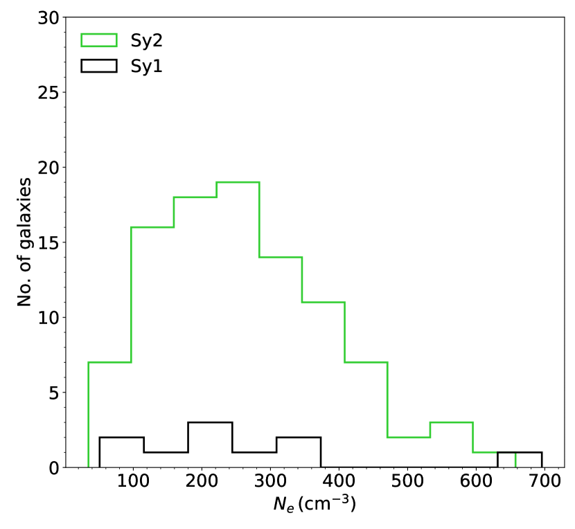
Figure 2: Electronic density distributions obtained within the 2.5 arcsec central region for the 107 AGN of our sample. The distribution for Seyfert 1 and Seyfert 2 are represented in black and green colors, respectively.

In Fig. 2 we present the electron density distribution obtained within the 2.5 arcsec central region, for the 108 Seyfert galaxies. The black and green distributions represent the results for Seyfert 1 and Seyfert 2 nuclei, respectively. The maximum and minimum values, taking into account the total sample of Seyfert 1 and Seyfert 2, are 696 cm^-3 and 35 cm^-3 respectively, with the mean value of $N_{\rm e}$ $\approx$ 260 cm^-3 and a median value of $N_{\rm e}$ $\approx$ 240 cm^-3. The range of $N_{\rm e}$ values derived from our sample is somewhat lower than the $N_{\rm e}$ values obtained by Dors et al. (2020), who derived the range $100\>\la\>N_{\rm e}\>(\rm cm^{-3})\>\la\>10\,000$ and an average value of $\sim 650$ cm^-3, for a sample of 463 Seyfert 2 nuclei whose data were taken from the SDSS DR7 (York et al., 2000). However, only 15 % of the objects considered by Dors et al. (2020) present higher $N_{\rm e}$ values than the maximum value derived from our sample. Vaona et al. (2012) selected about 2 700 spectra of Seyfert nuclei from SDSS DR7 (York et al., 2000) and, among other nebular properties, estimated $N_{\rm e}$ mainly based on the [S ii]$\lambda 6716/6731$ line ratio. These authors derived a range of values similar to the estimations by Dors et al. (2020) and an average value of $N_{\rm e}\sim 250$ cm^-3, whereby most of the objects ($\sim 2\,300$ galaxies) show values lower than 500 cm^-3, while higher electron density values greater than 1000 cm^-3 were derived from only 97 ($\sim 3\,\%$) objects (see also Zhang et al. 2013). Thus, the discrepancy in $N_{\rm e}$ values above is probably due to the distinct and larger sample of objects considered by Dors et al. (2020) and Vaona et al. (2012). It is worth to mention that the $N_{\rm e}$ values obtained from our sample are well below the critical density value ($N_{\rm c}$) of the emission-lines considered in the present work. In fact, the emission line with the lowest $N_{\rm c}$ is [S ii]$\lambda$6716 ($N_{\rm c}\sim 1600\rm\>cm^{-3}$, Vaona et al. 2012), indicating that the collisional de-excitation is negligible in this case, which also does not affect the emissivity of the lines and, consequently the chemical abundance estimations (for a detailed discussion on electron density effects on AGN abundance determinations see Dors et al. 2020a).

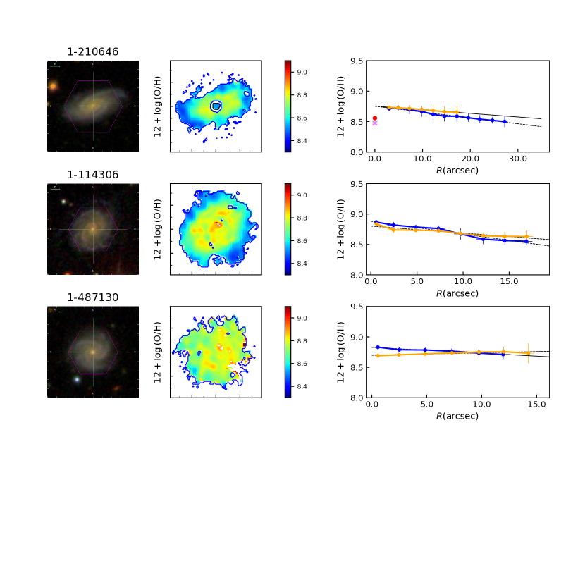
Figure 3: Surface distribution of the gas abundances for the Seyfert 2 galaxy MANGA ID 1-210646 (top row) and its two controls (bottom rows). The tick marks in the maps are separated by 5^′′. The left column shows the SDSS-IV images in the bands gri with the MaNGA footprint over-plotted in pink for the AGN (top) and its controls (bottom); central column: the metallicity distribution derived assuming the Carvalho et al. (2020) calibration for the AGN region (top row) and the Pérez-Montero & Contini (2009) calibrations for the HII regions in the disk of both the AGN and control galaxies (bottom rows); right column: mean azymuthal profile and standard deviations of the oxygen abundance [in units of 12+log(O/H)]. The profile in blue was obtained from Eq. 4 and the one in orange was obtained from Eq. 6, and are plotted versus the galactocentric distance $R$ (in units of arcsec). In the top panel showing the AGN gradient, the central values obtained from the calibration proposed by Carvalho et al. (2020) and Storchi-Bergmann et al. (1998) are shown in red point and pink cross sign point, respectively.

We derived spatially resolved maps and radial chemical abundance profiles for the AGN together with controls and showing the corresponding maps for the galaxy with MaNGA ID 1-210646 (AGN) and its controls in Fig. 3. The maps for the remaining objects are shown in Figures A1 - A72 in the Appendix. The radial profiles were corrected for projection, using information about the major and minor axis (from SDSS galaxy image, obtained from the MaNGA’s drpall table) to determine the inclination of the galaxies. The inclination angle of the AGN sample and their controls range from 1 to 70 degrees (the control galaxies were chosen to match each of the selected AGN hosts). We were able to obtain the O/H radial gradients for 61 galaxies containing AGNs (from a total sample of 108 galaxies hosting AGNs) and for 112 control galaxies (from a sample of 145 control galaxies). The chemical abundance profiles shown in blue and orange in Figs. 3 and A1 - A72 were derived by using the calibrations (Eqs. 4 and  6) from Pérez-Montero & Contini (2009). The dashed lines represent the fits of the points by Eq. 7. The blue and orange points represent the mean values, with standard deviations, considering all spaxels (both from control and AGN galaxies) divided in bins of 2.5 arcsec width. The slopes of the gradients in each galaxy and extrapolated abundances [$Y_{0}\rm\equiv 12+log(O/H)_{0}$] to the center (galactocentric distance $R=0$) are listed in Table 1.

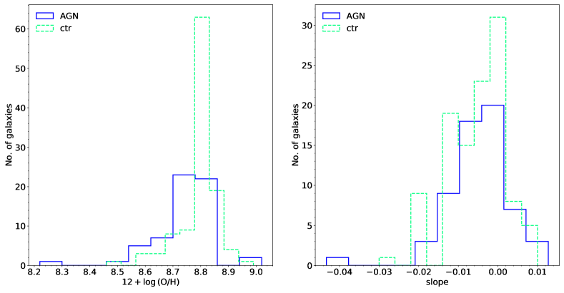
Figure 4: Left: distribution of nuclear chemical abundance obtained using the extrapolation method for AGNs and their control galaxies. Both were obtained from the use of the $N2$ calibration in the H ii regions. Right: histogram of the slopes of the abundance gradients for the AGNs compared to those from their control galaxies. AGN are shown in blue and the controls in light green dashed lines.

Fig. 3 and Figs. A1 - A72 show, in the left panels, SDSS image in the bands gri of each galaxy with the MaNGA footprint over-plotted in pink, and in the central panels, maps of the oxygen abundance distribution [in units of 12+log(O/H)] along the galactic disks.

The white regions in these maps represent the spaxels classified as transition objects or LI(N)ER-like objects (see also Kaplan et al. 2016) for which the calibrations used in this work can not be applied. Although recent studies (Kumari et al., 2019; Wu, 2020, 2021) have investigated metallicity derivation in these object class, we did not obtain any estimate for them. For about 43 % of the AGN sample it was not possible to obtain the radial abundance gradient due to the fact that the spaxels in the disk are not classified as SF-like objects in the diagnostic diagram (see Fig. 1), i.e. they are classified as transition or AGN-like objects. These objects may include disk regions with a composite ionization source, such as shocks mixed with ionization from a young stellar cluster (e.g. see Allen et al. 2008; Rosa et al. 2014). Transition objects are indeed expected to have a stellar cluster–AGN mixing as their ionizing source (e.g. Kewley et al. 2006; Wu et al. 2007; Davies et al. 2014). Although recent studies have proposed methods to estimate the metallicity in this class of objects (i.e. composite objects, see for instance Wu 2020, 2021), we did not estimate the abundances for them because the main goal of this work is the comparison between AGN and H ii region metallicities.

Regarding the metallicity gradients presented in the right panels of Fig 3 and Figs. A1 - A72 (for the AGN host disk and its control galaxies), we can state that: in the AGN host disk, the metallicity gradient is comparable to that found in the control galaxies; although we have used two different calibrations for the H ii regions – the blue profile derived from the $O3N2$ index (Eq. 5) and the orange profile from the $N2$ index (Eq. 6) – show similar gradients that are mostly negative. Our main findings are:

• $\sim$66 % of the galaxies containing AGNs have negative radial gradients when these are derived via $O3N2$ and $N2$ indices (i.e. the O/H abundance decreases as the galactocentric distance increases);

• $\sim$25 % of AGN hosts have positive gradients, indicating an increase in metallicity as we move away from the central region; and

• $\sim$9 % of the AGN host sample present flat gradients.

These results are confirmed by the histograms shown in Fig. 4, comparing the central extrapolated abundances and the gradient slopes of the AGN hosts (blue line) with those from their control galaxies (light green dashed lines).

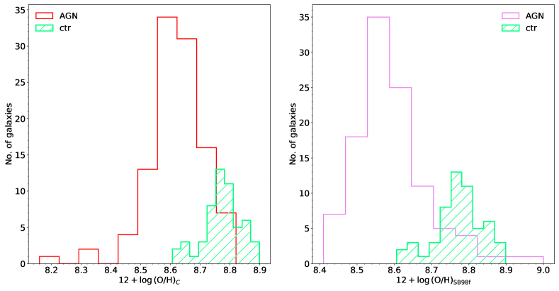
Figure 5: Histograms showing the central oxygen abundances distribution for the AGNs compared to that of the control galaxies. In the left panel, the AGN abundances were obtained using the Carvalho et al. (2020) calibration (red open histogram) and in the right panel, using the Storchi-Bergmann et al. (1998) calibration (pink open histogram). The control galaxies are represented by the hatched histogram in light green.

If galaxies evolve as a closed system and are formed according to the inside-out scenario (e.g. Mollá & Díaz 2005), negative abundance gradients are expected. In fact, this feature is commonly found in most disks of spiral galaxies (e.g. Shaver et al. 1983; van Zee et al. 1998; Kennicutt et al. 2003; Pilyugin et al. 2004; Dors & Copetti 2005; Sánchez et al. 2014; Belfiore et al. 2017; Skillman et al. 2020; Mingozzi et al. 2020). However, some relevant processes could affect the galaxy evolution resulting in radial gradients which differ from the expected negative abundance gradients. For instance, some galaxies are formed and evolve in a complex environment (galaxies can have a nurture evolution; see Paulino-Afonso et al. 2019 and references therein), with gas circulating inside, outside and around of them, making galaxies evolve in short time scales (Somerville & Davé, 2015). This cycle includes modified star-formation, accretion, mergers, and the way each action impacts the galaxy is unique. If metal-poor gas accretion is deposited directly into the centers of galaxies, it should act to dilute the central metallicity, flatten or push down negative gradients (Simons et al., 2020), producing a break in the gradients at small galactocentric distances.

The histograms in Fig. 5 show the oxygen abundance distributions calculated within the inner 2.5 arcsec of each galaxy, i.e for the AGNs and their control galaxies (which have star-forming nuclei), whose O/H values were derived by using the calibrations described in Sect. 2. In the left and right panels of Fig. 5 the AGNs abundances calculated by Eqs. 12 and 13 are represented in red and pink colours, respectively. Distributions for the control sample are represented by the hatched area (in light green) and the abundances are estimated using Eq. 5. In both panels of Fig. 5, it can be seen that the results indicate that control galaxies present O/H abundance values higher than those derived for AGNs.

In Fig. 6, the $\rm 12+\log(O/H)$ values obtained from the AGN calibrations (see Sect. 2.4) are plotted against those inferred from the gradient extrapolations. The $Y_{0}$ values (see Eq. 7) of the metallicity gradients were determined from the H ii region calibrations based on $O3N2$ (left panels) and $N2$ (right panels) indices proposed by Pérez-Montero & Contini (2009). In general, it is possible to verify that, even considering the errors in the estimates, i.e. in order of $\pm 0.1$ dex (e.g. Denicoló, Terlevich & Terlevich 2002; Marino et al. 2013), the direct estimations for AGNs (derived through Storchi-Bergmann et al. (1998) and Carvalho et al. (2020) calibrations) are lower than the estimates obtained from the gradient extrapolations for the high metallicity regime ($\rm 12+\log(O/H)\>\ga\>8.6$). Our findings reveal that:

• $\sim$80 % of the metallicity values of AGNs, derived from the Storchi-Bergmann et al. (1998) and Carvalho et al. (2020) calibrations are lower than those obtained via extrapolation methods (using both the $N2$ and $O3N2$ relations for the H ii regions to derive the disk gradients);

• $\sim$15 % of the metallicity values obtained for the AGNs are similar (within the uncertainties) to those obtained via the extrapolation estimates; and

• for $\sim$5 % of the sample we found the AGN metallicities derived from the calibrations above higher than the values derived from the extrapolations.

In Fig. 3, both the O/H radial gradients and the estimates for the AGN (based on Storchi-Bergmann et al. 1998 and Carvalho et al. 2020 calibrations) for the Seyfert 2 galaxy with MANGA ID 1-210646 are shown. It can be seen that a break in the radial gradient at small galactocentric distance is observed when considering the values based on the AGN calibrations, while the difference between the two values (or discrepancy) $D$ is of the order of 0.5 dex (see also Fig. 7). In summary, there is a clear tendency of the AGN oxygen abundance (or metallicity) to be lower than the extrapolated O/H value for the high metallicity regime.

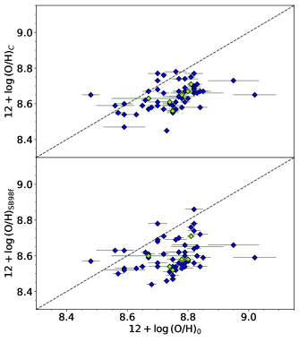
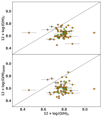
Figure 6: Left panels: $\rm 12+\log(O/H)$ calculated from Carvalho et al. (2020) (top panel) and Storchi-Bergmann et al. (1998) (bottom panel) vs. $\rm 12+\log(O/H)_{0}$ calculated from the O3N2 calibration for the H ii regions of PMC09. Right panels: $\rm 12+\log(O/H)$ calculated from Carvalho et al. (2020) (top panel) and Storchi-Bergmann et al. (1998) (bottom panel) vs. $\rm 12+\log(O/H)_{0}$ calculated from the N2 calibration for the H ii regions of PMC09. The solid line represents the equality between the estimates.

The above result is in agreement with some results found in previous studies. For instance, Dors et al. (2015), who used long-slit spectroscopic data obtained by Ho et al. (1997), found that the metallicity in the NLR (derived from Storchi-Bergmann et al. 1998 calibration) and in star-forming nuclei, whose metallicity was estimated by using the $C$-method (Pilyugin et al., 2012, 2013), are close to or slightly lower than those obtained by the extrapolation method in the regime of high metallicity, i.e. 12+log(O/H)$\ga\>8.6$. These authors pointed out that metal-poor gas accretion is less evident for galaxies with low-metallicity, where the metallicity of the accretion material is similar (or not so different) to that of the gas phase in the central regions, therefore, not producing significantly metallicity change. The opposite, probably, occurs for AGNs with high metallicity, where the infalling poor metallicity gas and the one in the galaxy differ considerably. This scenario explains the result shown in Fig. 6. Sánchez et al. (2014) found, for $\sim$10 % of the objects of the their sample, observational evidence of lower central oxygen abundances than those inferred from the O/H gradient extrapolation to the central parts of spiral galaxies and suggested that a possible explanation is the addition of metal-poor gas to the center of the galaxies.

To verify if the result shown in Fig. 6 is dependent on the calibration assumed to derive the O/H gradients in our sample, other empirical calibrations were also considered. In particular, we considered the empirical calibrations proposed by Denicoló, Terlevich & Terlevich (2002):

$$\mathrm{12+\log(O/H)}=9.12+0.73\times N2,$$ (16)

and by Pettini & Pagel (2004):

$$\mathrm{12+\log(O/H)}=8.90+0.57\times N2,$$ (17)

and calculated the radial gradients for all objects in our sample.

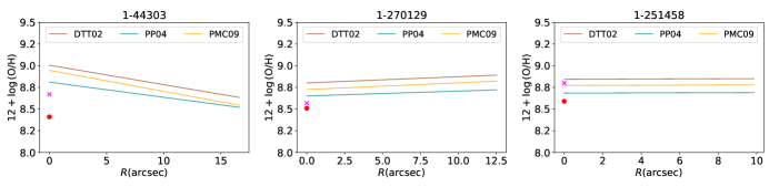
Figure 7: Radial profiles of $\rm 12+\log(O/H)$ obtained by using three different metallicity calibrations for star-forming regions. The lines represent linear regression to the points (not shown): the brown, dark cyan and orange lines represent linear regressions to the O/H abundance estimates for disk H ii regions of each object obtained assuming the calibration by Denicoló, Terlevich & Terlevich (2002) - DTT02 (Eq. 16), Pettini & Pagel (2004) - PP04 (Eq. 17) and Pérez-Montero & Contini (2009) - PMC09 (Eq. 6), respectively. The red point and pink cross sign points represent the abundances for AGN calculated via Carvalho et al. (2020) (Eq. 13) and Storchi-Bergmann et al. (1998) (Eq. 11) calibrations, respectively. The error in O/H abundances derived from strong emission line line calibrations is of the order of $\pm 0.1$ dex (Denicoló, Terlevich & Terlevich, 2002).

In Fig. 7, we show the abundance gradients as well as the nuclear abundance values for three AGN hosts, with MANGA ID’s 1-44303, 1-270129 and 1-251458, which are representative of the abundance profiles observed in our sample. The resulting O/H gradients based on the three calibrations above are represented by lines with different colours. These gradients were extrapolated to the zero galactocentric distance ($R=0$). In Fig. 7, the 12+log(O/H) values obtained for the AGNs using the Carvalho et al. (2020) and Storchi-Bergmann et al. (1998) calibrations are also indicated as a red dot and purple cross, respectively. It can be seen that, independently from the calibration considered to derive the gradients in the AGN, with exception of the object 1-251458, for which the Storchi-Bergmann et al. (1998) calibration produces a high O/H value, we confirm that the extrapolated values are usually higher than those derived from the AGN calibrations. Moreover, the error associated with O/H estimates from calibrations based on strong emission lines is in the order of $\pm$0.1 dex (e.g. Denicoló, Terlevich & Terlevich 2002; Marino et al. 2013), lower than the average discrepancy $<D>$ (see below) derived for our sample. The rest of the objects (not shown) were subjected to the same process as those in Fig. 7 and yielded similar results.

As discussed previously, there are several physical processes that can produce a decrease (or different O/H abundances) in the O/H abundance (or $Z$) in the central parts of galaxies in comparison with that obtained from the gradient extrapolation. The simplest scenario appears to be the accretion of metal-poor gas into the nuclear region, e.g. via the capture of a gas rich dwarf galaxy, which is a process that can lead to the triggering of nuclear activity in galaxies, as discussed in Storchi-Bergmann & Schnorr-Müller (2019). A molecular (e.g. Riffel et al. 2008, 2013, Moiré et al. 2018) and/or neutral gas (e.g. Allison et al. 2015) reservoir can thus form in the surroundings of the supermassive black hole (SMBH), feeding it.

Some recent studies have pointed out that star formation inside AGN gas outflows (e.g. Gallagher et al. 2019) and/or supernova explosions in accretion disks can locally enrich the AGN and produce very high abundances, mainly in the Broad Line Regions (e.g. Wang et al. 2011; Moranchel-Basurto et al. 2021). But, in our case, we find low metallicity in the NLRs of the sample, and therefore, the most likely process is that we are observing an accretion of poor metal gas rather than a higher star formation rate in the innermost disk H ii regions.

In order to investigate if there is any correlation between the oxygen discrepancy $D$, derived by using Eq. 15, and relevant physical properties of the AGN sample, in Fig. 8 we plot the electron density of the AGN NLR, luminosity of H$\alpha$ and the extinction coefficient $A_{\rm v}$ obtained within the inner 2.5 arcsec versus $D$. In addition, the luminosity of [O iii]$\lambda$5007 and stellar masses derived from SDSS-III data (Thomas et al., 2013) were also plotted versus $D$ in the second column of Fig. 8. The blue and orange symbols represent which calibration was considered in the radial extrapolation: blue for the $O3N2$ calibration and orange for the $N2$ calibration of PMC09. A linear regression to the points in each plot of Fig. 8 was performed. The best fit coefficients, the Pearson Correlation Coefficient (R) and the $p$ value are listed in Tables 3 and  4. The O/H abundances in the AGNs were those obtained through Carvalho et al. (2020) because this calibration considers a wider range of nebular parameters than that of Storchi-Bergmann et al. (1998). Based on the linear fits, $R$ and $p$ values and from the analysis of the plots in Fig. 8, we can state that for the $O3N2$ calibration (represented by blue symbols), there is no correlation between the AGN and galaxy properties and $D$. The $p$ value confirms that R is not significant (considering the level of significance as $p\leq$0.05). On the other hand, for the $N2$ calibration (represented by orange symbols), there is evidence of a mild inverse correlation between the following properties and $D$: electron density, stellar mass and extinction $A_{\rm v}$. The cause of these inverse correlations is not clear.

It is worthwhile to stress again that, the oxygen abundance estimations via strong line methods for H ii regions and AGNs can differ from each other up to $\sim 0.8$ dex (e.g. Kewley & Ellison 2008; Dors et al. 2020b). Thus, to confirm the non-existence of correlation between AGN nebular parameters and $D$ found above it is necessary to estimate the O/H gradients and AGN abundances based on direct estimations of the electron temperature, i.e. by using the $T_{\rm e}$-method (the most reliable method), which is not possible considering the data in this paper.

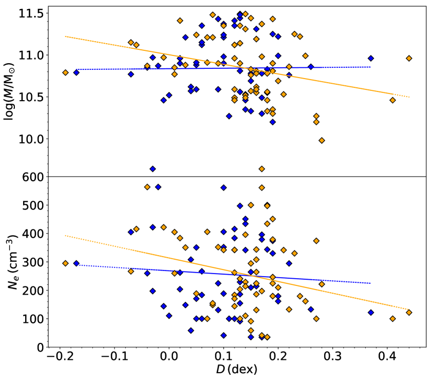
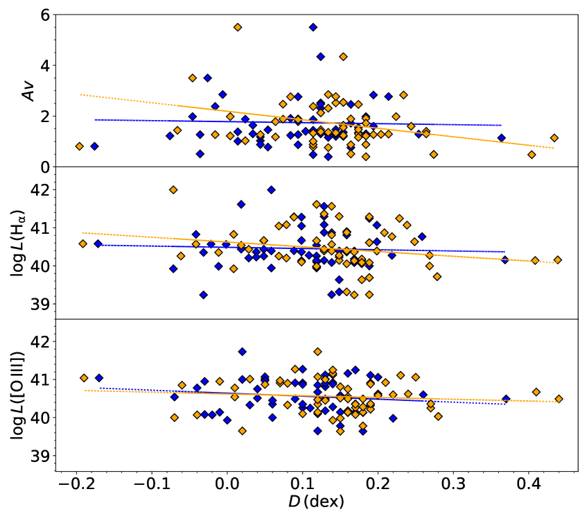
Figure 8: Left panels: Electron density (in units of cm^-3) for each AGN NLR and the logarithm of the stellar mass of the hosting galaxy versus the difference D (in dex, Eq. 15) between the O/H abundance of the AGN (derived from Carvalho et al. 2020 calibration – Eq. 13) and the intersect oxygen abundances derived from the radial abundance gradients – blue symbols for the HII O3N2 calibration and orange symbols for the N2 calibration of PMC09. Rigth panels: As in the left panels but for the logarithm of the luminosity of [O iii]$\lambda$5007 and H$\alpha$ as well as the extinction $A_{\rm v}$ (in units of magnitude) of the AGNs. Blue and orange lines represent a linear regression to the corresponding points. The linear regression coefficients as well as the Pearson Correlation Coefficients (R) and p-values for the blue points are listed in Table 3, while those for the orange points are listed in Table 4.

Table 3: Coefficients of the linear regression to the blue symbols (O3N2 HII regions O/H calibration) shown Fig. 8 and the corresponding Pearson Correlation Coefficient (R) and the $p$-value.

	a	b	R	$p$
$N_{\rm e}$ (cm-3)	$-$119$\pm 194.1$	268.8$\pm 27.19$	$-$0.08	0.54
log($M/{\rm M_{\odot}}$)	$0.05\pm 0.57$	10.84$\pm 0.08$	$-$0.01	0.93
log$L$([O iii])	$-$0.79$\pm 0.63$	40.64$\pm 0.09$	$-$0.16.	0.22
log$L$(H$\alpha$)	$-$0.32$\pm 0.83$	40.49$\pm 0.12$	$-$0.05	0.70
$A_{\rm v}$	$-$0.40$\pm 1.58$	1.78$\pm 0.22$	$-$0.03	0.82

Table 4: Coefficients of the linear regression to the orange symbols (N2 HII regions O/H calibration) shown Fig. 8, the corresponding Pearson Correlation Coefficient (R) and the $p$-value.

	a	b	R	$p$
$N_{\rm e}$ (cm-3)	$-$413.7$\pm 161.2$	313.8$\pm 27.87$	$-$0.32	0.01
log($M/{\rm M_{\odot}}$)	$-$1.15$\pm 0.48$	11$\pm 0.08$	$-$0.30	0.02
log$L$([O iii])	$-$0.47$\pm 0.56$	40.62$\pm 0.10$	$-$0.11.	0.41
log$L$(H$\alpha$)	$-$1.25$\pm 0.71$	40.63$\pm 0.12$	$-$0.22	0.09
$A_{\rm v}$	$-$3.35$\pm 1.31$	2.21$\pm 0.23$	$-$0.32	0.01

4 SUMMARY

We derived the metallicities of MaNGA AGN NLRs (traced by the O/H abundance) and the radial gradients of oxygen abundance along the disk for 98 Seyfert 2 and 10 Seyfert 1 host galaxies using MaNGA-SDSS-IV data cubes. The metallicities of the AGNs and in the disk of H ii regions were obtained using calibrations based on strong emission lines proposed in the literature. We derived for most galaxies clear O/H gradients, with the O/H abundance ratio decreasing as the galactocentric distance increases. This characteristic is commonly found in the disk of spiral galaxies, which suggest that most spiral galaxies are formed according to the inside-out scenario. The oxygen abundances derived through emission lines of the AGNs and based on two distinct calibrations are lower by an average value $<D>$ of 0.16-0.30 dex (depending on the calibration assumed) than the extrapolated oxygen abundances to the central parts derived from the radial abundance gradients. We suggest that the difference $<D>$ can be due to the accretion of metal-poor gas to the AGN host – probably via the capture of a gas-rich dwarf galaxy, that builds up a reservoir of molecular and/or neutral gas which will then feed the SMBH. This gas will then trigger the nuclear acitivity via its capture by the nuclear supermassive black hole (SMBH). We investigated correlations between $D$ and the electron density ($N_{\rm e}$), [O iii]$\lambda$5007 and H$\alpha$ luminosities, extinction coefficient ($A_{V})$ of the AGN as well as the stellar mass ($M_{*}$)of the hosting galaxy. We did not find any significant correlation between the aforementioned properties and $D$ when the oxygen gradients are derived from $O3N2$ index. Otherwise, there is evidence of an inverse correlation between the $D$ and $N_{\rm e}$, $M_{*}$ and $A_{\rm v}$ when the $N2$ index is used. The origin of inconsistency observed here, probably, it is due to the use of different metallicity indicators to derive the radial gradients. To confirm the derived correlations, further investigation with oxygen radial gradients and AGN estimations based on direct determination of the electron temperature, i.e. by using the $T_{\rm e}$-method, is required.

Data Availability

The data underlying this article are available under SDSS collaboration rules, and the by products will be shared on reasonable request to the corresponding author.

Appendix A AGN maps

We present all the maps and gradients of the chemical abundances obtained from the calibrations for the AGNs and the controls, as well as the extrapolations in Figs. A1 - A75.

See pages - of appendix/supplementary_figures.pdf

References

- Aguado et al. (2019) Aguado D. S., Ahumada R., Almeida A., Anderson S. F., Andrews B. H., Anguiano B., Aquino Ortíz E., et al., 2019, ApJS, 240, 23.
- Allen et al. (2008) Allen M. G., Groves B. A., Dopita M. A., Sutherland R. S., Kewley L.J., 2008, ApJS, 178, 20
- Allen et al. (2015) Allen J. T., Schaefer A. L., Scott N. et al., 2015, MNRAS, 451, 2780
- Alende Pietro, Lambert & Asplund (2001) Alende Prieto C., Lambert D. L., Asplund M., 2001, ApJ, 556, L63
- Allison et al. (2015) Allison J. R., Sadler E. M., Moss V. A. et al., 2015, MNRAS, 453, 1249
- Alloin, et al. (1979) Alloin D., Collin-Souffrin S., Joly M., Vigroux L., 1979, A&A, 78, 200
- Baldwin, Phillips & Terlevich (1981) Baldwin, J.A., Phillips, M.M., Terlevich, R., 1981, PASP,93, 5
- Belfiore et al. (2017) Belfiore F., Maiolino R., Tremonti C. et al., 2017, MNRAS, 469, 151
- Berg et al. (2015) Berg D. A., Skillman, E. D., Croxall K. V., Pogge R. W., Moustakas J., Johnson-Groh M., 2015, ApJ, 806, 16
- Berg et al. (2020) Berg D. A., Pogge, R. W., Skillman, E. D., Croxall K. V., Moustakas J., Rogers Noah S. J., Sun, J., 2020, ApJ, 893, 96
- Blanton et al. (2017) Blanton M. R., Bershady M. A., Abolfathi B., Albareti F. D., Allende Prieto C., Almeida A., Alonso-García J., et al., 2017, AJ, 154, 28
- Bundy et al. (2015) Bundy, K., et al., 2015, ApJ 798, id. 7
- Buzzo et al. (2021) Buzzo, M. L.; Ziegler, B.; Amram, P.; Verdugo, M.; Barbosa, C. E.; Ciocan, B.; Papaderos, P.; Torres-Flores, S.; Mendes de Oliveira, C.
- Carvalho et al. (2020) Carvalho S.P., et al., 2020, MNRAS, 492, 5675
- Castro et al. (2017) Castro C. S., Dors O. L., Cardaci M. V., Hägele G. F., 2017, MNRAS, 467, 1507
- Cid Fernandes et al. (2010) Cid Fernandes, R., Stasińska, G., Schlickmann, M. S., Mateus, A., Vale Asari, N., Schoenell, W., Sodrhoenell, W., Sodré 2010, L.2010,MNRAS, 403, 1036
- Comerford & Greene (2014) Comerford J. M., & Greene J. E., 2014, ApJ, 789, 112
- Congiu et al. (2017) Congiu, E.; Contini, M.; Ciroi, S.; Cracco, V.; Berton, M.; Di Mille, F.; Frezzato, M.; La Mura, G.; Rafanelli, P., 2017, MNRAS, 471, 562
- Cresci et al. (2015) Cresci, G., Mannucci, F., Maiolino, R., et al. 2010, Nature, 467, 811
- Croxall et al. (2015) Croxall K. V., Pogge R. W., Berg D. A., Skillman E. D., Moustakas J., 2015, ApJ, 808, 42
- Croxall et al. (2016) Croxall K. V., Pogge R. W., Berg D. A., Skillman E. D., Moustakas J., 2016, ApJ, 830, 4
- Croom et al. (2012) Croom, S. M., Lawrence J. S., Bland-Hawthorn J. et al., 2012, MNRAS, 421, 872
- Copetti et al. (2000) Copetti, M. V. F.; Mallmann, J. A. H.; Schmidt, A. A.; Castañeda, H. O., 2000, A&A, 357, 621
- Davies et al. (2014) Davies R. L., Kewley L. S., Ho I-T., Dopita M., 2014, MNRAS, 444, 3961
- Davies et al. (2020) Davies R., Baron D., Shimizu T., Netzer H., Burtscher L., de Zeeuw P. T., Genzel R., et al., 2020, MNRAS, 498, 4150
- Denicoló, Terlevich & Terlevich (2002) Denicoló G., Terlevich R., Terlevich E., 2002, MNRAS, 330, 69.
- Dors & Copetti (2005) Dors O. L., & Copetti M. V. F., 2005, A&A, 437, 837
- Dors et al. (2014) Dors O. L., Cardaci M. V., Hägele G. F., Krabbe Â. C., 2014, MNRAS, 443, 1291
- Dors et al. (2015) Dors O. L., et al., 2015, MNRAS, 453, 4102
- Dors et al. (2017) Dors O. L., H¨agele G. F., Cardaci M. V., Krabbe A. C., 2017a, MNRAS, 466, 726
- Dors et al. (2017b) Dors O. L., Arellano-Córdova K. Z., Cardaci M. V., Hägele G. F., 2017b, MNRAS, 468, L113
- Dors et al. (2018) Dors O. L., Agarwal B., Hägele G. F., Cardaci M. V., Rydberg C., Riffel R. A., Oliveira A. S., Krabbe A. C., 2018, MNRAS, 479, 2294
- Dors et al. (2019) Dors O. L., Monteiro A. F, Cardaci M. V., Hägele G. F., Krabbe Â. C., 2019, MNRAS, 486, 5853
- Dors et al. (2020) Dors O. L., Freitas-Lemes P., Amôres E. B., Pérez-Montero E., Cardaci M. V., Hägele G. F., Armah M., et al., 2020, MNRAS, 492, 468
- Dors et al. (2020a) Dors O. L., Maiolino R., Cardaci M. V., Hagele G. F.; Krabbe A. C., Perez-Montero E. Armah M., 2020a, MNRAS, 496, 3209
- Dors et al. (2020b) Dors O. L., Freitas-Lemes P., Amôres E. B. et al., 2020, MNRAS 492, 468
- Dors et al. (2021) Dors O. L., Contini M., Riffel R. A., Pérez-Montero E., Krabbe A. C., Cardaci M. V., Hägele G. F., 2021, MNRAS, 501, 1370
- Dors (2021) Dors, O. L., 2021, MNRAS, 507, 466
- do Nascimento et al. (2019) do Nascimento J. C., et al., 2019, MNRAS, 486, 5075
- Drory et al. (2015) Drory, N., MacDonald, N., Bershady, M. A., et al. 2015, AJ, 149, 77
- Esteban et al. (1998) Esteban C., Peimbert M., Torres-Peimbert S., Escalante V., 1998, MNRAS, 295, 401
- Feltre, Charlot & Gutkin (2016) Feltre A., Charlot S., Gutkin J., 2016, MNRAS, 456, 3354
- Ferland & Netzer (1983) Ferland G. J., & Netzer H., 1983, ApJ, ApJ, 264, 105
- Ferland & Osterbrock (1986) Ferland G. J., & Osterbrock D. E., 1986, ApJ, 300, 658
- Ferland et al. (1998) Ferland G. J., Korista K. T., Verner D. A., Ferguson J. W., Kingdon J. B., Verner E. M., 1998, PASP, 110, 761
- Ferland et al. (2017) Ferland G. J., 2017, Rev. Mex. Astron. Astrofis., 53,385
- Freitas et al. (2018) Freitas, I. C.; Riffel, R. A.; Storchi-Bergmann, T.; Elvis, M.; Robinson, A.; Crenshaw, D. M.; Nagar, N. M.; Lena, D.; Schmitt, H. R.; Kraemer, S. B., 2018, MNRAS, 476, 2760
- Flury & Moran (2020) Flury S. R., & Moran E. C., 2020, MNRAS, 496, 2191
- Gallagher et al. (2019) Gallagher R., Maiolino R., Belfiore F., Drory N., Riffel R., Riffel R. A., MNRAS, 485, 3409
- Gillman et al. (2021) Gillman S., Tiley A. L., Swinbank A. M. et al., 2021, MNRAS, 500, 4229
- Guo et al. (2020) Guo Y. et al., 2020, ApJ, 898, 26
- Gunn et al. (2006) Gunn, J. E., Siegmund, W. A., Mannery, E. J., et al. 2006, AJ, 131, 2332
- Groves, Heckman & Kauffman (2006) Groves B. A., Heckman T. M., Kauffmann G., 2006, MNRAS, 371, 1559
- Hagele et al. (2008) Hagele G. F., Dıaz A. I., Terlevich E., Terlevich R., Perez-Montero E., Cardaci M. V., 2008, MNRAS, 383, 209
- Hampton et al. (2017) Hampton E. J., Medling A. M. et al., 2017, MNRAS, 470, 3395
- Ho et al. (1997) Ho L. C., Filippenko A. V., Sargent W. L. W., 1997, ApJS, 112, 315
- Ilha et al. (2019) Ilha G. S., Riffel R. A., Schimoia J. S., Storchi-Bergmann T., Rembold S. B., Riffel R., Wylezalek D., et al., 2019, MNRAS, 484, 252
- Izotov et al. (2006) Izotov Y. I., Stasińska G., Meynet G., Guseva N. G., Thuan, T. X., 2006, A&A, 448, 955
- Jenkins (2009) Jenkins E. B. 2009, ApJ, 700, 1299
- Ji et al. (2020) Ji X., Yan R., Riffel R., Drory N., Zhang K., 2020, MNRAS, 496, 1262
- Kaddad et al. (2018) Kakkad, D.; Groves, B.; Dopita, M.; Thomas, A. D.; Davies, R. L.; Mainieri, V.; Kharb, P.; Scharwächter, J.; Hampton, E. J.; Ho, I. -T., 2018, A&A, 618, 6
- Kaplan et al. (2016) Kaplan K. F.,; Jogee S., Kewley L. et al., 2016, MNRAS, 462, 1642
- Kauffmann et al. (2003) Kauffmann G., Heckman T. M., Tremonti C., et al., 2003, MNRAS, 346, 1055
- Kennicutt et al. (2003) Kennicutt R. C., Bresolin F., Garnett D. R., 2003, ApJ, 591, 801
- Kewley et al. (2001) Kewley L. J., Dopita M. A., Sutherland R. S., Heisler C. A., Trevena J., 2001, ApJ, 556, 121
- Kewley et al. (2006) Kewley L. J., Groves B., Kauffmann G., Heckman T., 2006, MNRAS, 372, 961
- Kewley & Ellison (2008) Kewley L. J., Ellison S. L., 2008, ApJ, 681, 1183
- Krabbe et al. (2014) Krabbe A. C., Rosa D. A., Dors O. L., Pastoriza M. G., Winge C., Hagele G. F., Cardaci M. V., Rodrigues I., 2014, MNRAS, 437, 1155
- Krabbe et al. (2021) Krabbe, A. C., Oliveira C. B., Zinchenko I. A. et al., 2021, MNRAS, 505, 2087
- Kumari, James, & Irwin (2017) Kumari N., James B. L., Irwin M. J., 2017, MNRAS, 470, 4618. doi:10.1093/mnras/stx1414
- Kumari et al. (2019) Kumari N., Maiolino R., Belfiore F., Curti, M., 2019, MNRAS, 485, 367
- Law et al. (2015) Law, D. R., Yan, R., Bershady, M. A., et al. 2015, AJ, 150, 19
- Law et al. (2016) Law D. R., Cherinka B., Yan R., Andrews B. H., Bershady M. A., Bizyaev D., Blanc G. A., et al., 2016, AJ, 152, 83. doi:10.3847/0004-6256/152/4/83
- Lequeux et al. (1979) Lequeux J., Peimbert M., Rayo J. F., Serrano A., Torres-Peimbert S., 1979, A&A, 500, 145
- Lòpez-Sanchez et al. (2012) Lòpez-Sǹchez A. R., Dopita M. A., Kewley L. J., Zahid H. J., Nicholls D. C., Scharwachter J., 2012, MNRAS, 426, 2630
- Maiolino et al. (2008) Maiolino R. et al., 2008, A&A, 488, 463
- Mallmann et al. (2018) Mallmann, N. et al., 2018, MNRAS, 478, 5491.
- Marino et al. (2013) Marino, R. A. et al., 2013, A&A, 559, A114
- Matsuoka et al. (2009) Matsuoka K., Nagao T., Maiolino R., Marconi A., Taniguchi Y., 2009, A&A, 503, 721
- Matsuoka et al. (2018) Matsuoka, K. et al., 2018, A&A, 616, L4
- Meyer et al. (1998) Meyer D. M., Jura M., Cardelli J. A., 1998, ApJ, 493, 222
- Mignoli et al. (2019) Mignoli M. et al., 2019, A&A, 626, 9
- Mingozzi et al. (2020) Mingozzi, M.; Belfiore, F.; Cresci, G. et al., 2020, A&A, 636, 42
- Mingozzi et al. (2019) Mingozzi, M. et al., 2019, A&A, 622A, 146
- Moiré et al. (2018) Moiré H. G.; Riffel, Rogemar R. A.; Dors O. L., Riffel R.; Storchi-Bergmann T.; Colina, L., 2018, MNRAS, 477, 1086
- Mollá & Díaz (2005) Mollá M., & Díaz A. I., 2005, MNRAS, 358, 521
- Mora et al. (2019) Mora, M. D.; Torres-Flores, S.; Firpo, V.; Hernandez-Jimenez, J. A.; Urrutia-Viscarra, F.; Mendes de Oliveira, C., 2019, MNRAS, 488, 830
- Moranchel-Basurto et al. (2021) Moranchel-Basurto A., Sánchez-Salcedo F. J. Chametla R. O., Velázquez P. F., 2021, ApJ, 906, 15
- Nagao, Maiolino & Marconi et al. (2006) Nagao, T., Maiolino, R., Marconi, A., 2006, A&A, 447, 863
- Nakajima et al. (2018) Nakajima K. et al., 2018, A&A, 612, 94
- Lee & Skillman (2004) Lee H., & Skillman E. D., 2004, ApJ, 614, 698
- Pagel et al. (1979) Pagel B. E. J., Edmunds M. G., Blackwell D. E., Chun M. S., Smith, G., 1979, MNRAS, 189, 95
- Paulino-Afonso et al. (2019) Paulino-Afonso, A.; Sobral, D.; Darvish, B.; Ribeiro, B.; van der Wel, A.; Stott, J.; Buitrago, F.; Best, P.; Stroe, A.; Craig, J. E. M., 2019, A&A, 630, 57
- Peimbert et al. (2017) Peimbert M., ; Peimbert A., Delgado-Inglada G., 2017, PASP, 129, 2001
- Peña-Guerrero et al. (2012) Peña-Guerrero M. A., Peimbert A., Peimbert M., 2012, ApJ, 756, L14
- Perez-Montero & Diaz (2005) Perez-Montero E., Diaz A. I., 2005, yCat, J/MNRAS/361/1063
- Pérez-Montero & Contini (2009) Pérez-Montero E., Contini T., 2009, MNRAS, 398, 949
- Pérez-Montero (2017) Pérez-Montero E., 2017, PASP, 129, 3001
- Pérez-Montero et al. (2019) Pérez-Montero E. et al., 2019, MNRAS, 489, 2652
- Pettini & Pagel (2004) Pettini M., Pagel B. E. J., 2004, MNRAS, 348, L59.
- Pilyugin (2000) Pilyugin L. S., 2000, A&A, 362, 325
- Pilyugin (2001) Pilyugin L. S., 2001, A&A, 369, 594
- Pilyugin, Ferrini & Shkvarun (2003) Pilyugin L. S., Ferrini F., Shkvarun R. V., 2003, A&A, 401, 557
- Pilyugin et al. (2004) Pilyugin L. S., Vílchez J. M., Contini, T., 2004, A&A, 425, 849
- Pilyugin et al. (2012) Pilyugin L. S., Grebel E. K., Mattsson L., 2012, MNRAS, 424, 2316
- Pilyugin et al. (2013) Pilyugin L. S., Lara-López M. A., Grebel E. K., Kehrig C., Zinchenko I. A., López-Sánchez A . R., Vílchez J. M., Mattsson L., 2013, MNRAS, 432, 1217
- Rembold et al. (2017) Rembold, S. B., Shimoia, J. S., Storchi-Bergmann, T., et al. 2017, MNRAS, 472, 4382
- Revalski et al. (2018) Revalski M., Crenshaw D. M., Kraemer S. B., Fischer T. C., Schmitt H. R., Machuca C., 2018, ApJ, 856, 46
- Riffel et al. (2008) Riffel R. A.; Storchi-Bergmann T.; Winge C.; McGregor P. J.; Beck T.; Schmitt H., 2008, MNRAS, 385, 1129
- Riffel et al. (2013) Riffel R. A.; Storchi-Bergmann T.; Winge C., MNRAS, 430, 2249
- Riffel et al. (2021) Riffel R., Mallmann N. D., Ilha G. S., Storchi-Bergmann T., Riffel R. A., Rembold S. B., Bizyaev D., et al., 2021, MNRAS, 501, 4064.
- Riffel et al. (2021) Riffel R., Mallmann N. D., Ilha G. S., Storchi-Bergmann T., Riffel R. A., Rembold S. B., Bizyaev D., et al., 2021, MNRAS, 501, 4064.
- Rosa et al. (2021) Rosa, D. A.; Rodrigues, I.; Krabbe, A. C.; Milone, A. C.; Carvalho, S., 2021, MNRAS, 501, 3750
- Rosa et al. (2014) Rosa D. A., Dors O. L., Krabbe A. C.,Hagele G. F.,Cardaci M. V., Pastoriza M. G., Rodrigues I., Winge C., 2014, MNRAS, 444, 2005
- Richardson, et al. (2014) Richardson C. T., Allen J. T., Baldwin J. A., Hewett P. C., Ferland G. J., 2014, MNRAS, 437, 2376
- Rogers et al. (2021) Rogers N. S.J., Skillman E D., Pogge R. W.; Berg D. A.; Moustakas J., Croxall K. V., Sun J., 2021, ApJ, 915, 21
- Sánchez et al. (2014) Sánchez S. F. et al., 2014, A&A, 563, 49
- Sánchez et al. (2012) Sánchez S. F., Kennicutt R. C., Gil de Paz, A., et al. 2012, A&A, 538, A8
- Sarzi et al. (2006) Sarzi, M., Falcón-Barroso, J., Davies, R. L., et al. 2006, MNRAS, 366, 1151
- Shaver et al. (1983) Shaver P. A., McGee R. X., Newton L. M., Danks A. C., Pottasch, S. R., 1983, MNRAS, 204, 53
- Simons et al. (2020) Simons R. C., Papovich C., Momcheva I., Trump J. R., Brammer G., Estrada-Carpenter V., Backhaus B. E., et al., 2020
- Skillman et al. (2020) Skillman E. D., Berg D. A., Pogge R. W., Moustakas J., Rogers N. S. J., Croxall K. V., 2020, ApJ, 894, 138
- Smee et al. (2013) Smee S. A., Gunn J. E., Uomoto A., Roe N., Schlegel D., Rockosi C. M., Carr M. A., et al., 2013, AJ, 146, 32.
- Somerville & Davé (2015) Somerville R. S., Davé R., 2015, ARA&A, 53, 51.
- Skillman & Kennicutt (1993) Skillman E. D., & Kennicutt Robert C. J., 1993, ApJ, 411, 655
- Stasińska (1984) Stasińska G., 1984, A&A, 135, 341
- Sternberg et al. (1994) Sternberg A., Genzel R., Tacconi L., 1994, ApJ, 436, 131L
- Storchi-Bergmann, Calzetti, & Kinney (1994) Storchi-Bergmann T., Calzetti D., Kinney A. L., 1994, ApJ, 429, 572.