Linear and nonlinear waves in quantum plasmas with arbitrary degeneracy of electrons

Abstract

The purpose of this review is to revisit recent results in the literature where quantum plasmas with arbitrary degeneracy degree are considered. This is different from a frequent approach, where completely degeneracy is assumed in dense plasmas. The general reasoning in the reviewed works is to take a numerical coefficient in from of the Bohm potential term in quantum fluids, in order to fit the linear waves from quantum kinetic theory in the long wavelength limit. Moreover, the equation of state for the ideal Fermi gas is assumed, for arbitrary degeneracy degree. The quantum fluid equations allow the expedite derivation of weakly nonlinear equations from reductive perturbation theory. In this way, quantum Korteweg - de Vries and quantum Zakharov - Kuznetsov equations are derived, together with the conditions for bright and dark soliton propagation. Quantum ion-acoustic waves in unmagnetized and magnetized plasmas, together with magnetosonic waves, have been obtained for arbitrary degeneracy degree. The conditions for the application of the models, and the physical situations where the mixed dense - dilute systems exist, have been identified.

Keywords: degenerate plasma; quantum ion-acoustic wave; quantum Zakharov-Kuznetsov equation; quantum plasma with arbitrary degeneracy; quantum magnetosonic soliton.

I Introduction

It is customary in statistical mechanics of Fermions, to assume an equilibrium distribution function either of a completely degenerate Fermi gas or, in the extreme opposite, of a Maxwellian gas and therefore entirely neglecting the Fermi-Dirac statistics in this case. In quantum plasmas, the Fermi-Dirac character comes from electrons, among other possibilities. The completely degenerate case applies for $T\ll T_{F}$, where $T$ is the thermodynamic temperature and $T_{F}$ is the Fermi temperature. Correspondingly, the Maxwellian approximation is adequate for $T\gg T_{F}$, viz. for dilute, high temperature plasmas. Naturally, it is clear that in some instances there is not a clear separation between the temperature scales, so that one is obliged to consider the full Fermi-Dirac distribution for arbitrary degeneracy degree. The resulting mathematics becomes more involved, as in the case of the equation of state, now involving polylogarithm functions (Lewin 1981) and the presence of the chemical potential (Pathria and Beale 2011), besides number density. Intermediate regimes with $T\approx T_{F}$ appear in the plasma generated in inertial confinement (Manfredi and Hurst 2015) or laboratory simulation of high energy-density astrophysical plasmas which better fit the intermediate quantum-classical situation (Cross et al. 2014). The underlying full Fermi-Dirac distribution has consequence not only for the equation of state in a macroscopic, fluid-like system, but also on the quantum diffraction effects present in such hydrodynamics. The quantum diffraction effects manifest in quantum kinetic theory in the non-local form of the interaction term in the Wigner-Moyal equation or, in the quantum fluid equations, in the Bohm potential and higher-order gradient corrections (Haas 2011).

The purpose of this review is to present recent results in the literature, where the quantum hydrodynamics of arbitrary degeneracy plasmas was applied for the propagation of linear and nonlinear waves. The general approach behind these results is to assume the quantum hydrodynamic and quantum kinetic approaches should give the same linear dispersion relation in the long wavelength limit. This amounts to the introduction of a fitting parameter in the quantum dispersion or Bohm potential term. This is a different approach in comparison with other methods for quantum plasmas with arbitrary degeneracy. For instance, Maffa (1993) considered ion acoustic and Langmuir waves linearizing the Vlasov-Poisson system around a full Fermi-Dirac equilibrium, disregarding quantum diffraction. Including quantum recoil (or quantum diffraction), the low-frequency longitudinal plasma response for arbitrary degeneracy was studied (Mushtaq and Melrose 2009), (Melrose and Mushtaq 2010). Going from the linear to the nonlinear realm, Eliasson and Shukla (2008) take the first few moments of the Wigner-Moyal equation in terms of a local Fermi-Dirac distribution with arbitrary ratio $T/T_{F}$. Dubinov et al. (2010) used a Bernoulli pseudo-potential approach for warm Fermi gases, see also (Dubinov and Kitaev 2014). The screening potential around a test charge in a quantum plasma was studied using quantum hydrodynamics (QHD) in the linear limit with statistical (Fermi) pressure and Bohm potential from finite temperature kinetic theory (Eliasson & Akbari, 2016). The authors showed that the kinetic corrections included in the Bohm potential has a profound effect on the Thomas scattering cross section in a quantum plasma with arbitrary degeneracy and their theory is consistent with DFT theory in the limiting case of complete degeneracy of electrons.

The manuscript is organized as follows. In section 2 the basic quantum hydrodynamic equations for non-relativistic ion-acoustic waves in unmagnetized plasmas are reviewed, along with the equation of state, allowing arbitrary degeneracy. Linear waves are then investigated and compared to quantum kinetic results in the long wavelength limit. This amounts to the determination of a fitting parameter in front of the quantum dispersion term in the fluid equations. The propagation of weakly nonlinear waves is analyzed by means of the corresponding Korteweg - de Vries (KdV) equation, admitting arbitrary degeneracy level. Section 3 performs the same review as section 2, but now including an external uniform magnetic field. In consequence, the linear dispersion relation shows diverse new possibilities, for parallel, perpendicular and oblique wave propagation, besides strong magnetic fields. The agreement with quantum kinetic theory is shown again with the same equation of state and numerical coefficient in front of the Bohm potential term in quantum fluid equations, in the long wavelength limit. The weakly nonlinear theory in the magnetized case is given in terms of a quantum Zakharov-Kuznetsov equation, admitting soliton solutions among other possibilities. Section 4 reviews the propagation of magnetosonic waves in quantum plasmas with arbitrary degeneracy degree. The weakly nonlinear case is described in terms of the corresponding KdV equation derived from reductive perturbation methods. Section 5 address numerical estimates for suitable experiments in the intermediate dilute-degenerate regime, assuming the same values of Fermi and thermodynamic temperatures. Section 6 has some conclusions.

II Ion-acoustic Waves with Arbitrary Degeneracy Electrons in Unmagnetized Quantum Plasmas

In this section, the ion-acoustic waves in non-relativistic unmagnetized plasmas with arbitrary degeneracy of electrons are investigated. In this section mainly we review the material from (Haas and Mahmood 2015).

The continuity and momentum equations for non-degenerate ions are

$$\frac{\partial n_{i}}{\partial t}+\frac{\partial}{\partial x}(n_{i}u_{i}) =0\,,$$ (1)

$$\frac{\partial u_{i}}{\partial t}+u_{i}\frac{\partial u_{i}}{\partial x} =-\frac{e}{m_{i}}\frac{\partial\phi}{\partial x}\text{ }.$$ (2)

The momentum equation for the inertialess degenerate electron fluid is

$$0=e\frac{\partial\phi}{\partial x}-\frac{1}{n_{e}}\frac{\partial p}{\partial x}+\frac{\alpha\,\hslash^{2}}{6\,m_{e}}\frac{\partial}{\partial x}\left(\frac{1}{\sqrt{n_{e}}}\frac{\partial^{2}}{\partial x^{2}}\sqrt{n_{e}}\right)\,.$$ (3)

The Poisson equation is given by

$$\frac{\partial^{2}\phi}{\partial x^{2}}=\frac{e}{\varepsilon_{0}}(n_{e}-n_{i})\,.$$ (4)

In these equations $\phi$ is the electrostatic potential and $n_{i}$, $n_{e}$ are the ion and electron fluid density respectively while $u_{i}$ is the ion fluid velocity. Also, $m_{e}$ and $m_{i}$ are the electron and ion masses, $-e$ is the electronic charge, $\varepsilon_{0}$ the vacuum permittivity and $\hslash$ the reduced Planck’s constant. In electron momentum equation (3) $p=p(n_{e})$ is the electron’s fluid scalar pressure to be determined from a barotropic equation of state. The last term proportional to $\hslash^{2}$ in the momentum equation for electrons is the quantum force (or Bohm potential), responsible for quantum diffraction or quantum tunneling effects due to the wave like nature of the electrons. The extra dispersion effects appear through the Bohm potential. However a coefficient $\alpha$ appearing in Bohm potential term is selected in order to fit exactly in the long wavelength limit the linear dispersion relation obtained from kinetic theory in 3D Fermi-Dirac distributed electrons (Rubin et al. 1993). The definition of numerical factor $\alpha$ involves the dimensionality and temperature of the system (Barker and Ferry 1998) e.g., Gardner (1994) has obtained a factor $\alpha=1$ for a local Maxwell-Boltzmann equilibrium. In equilibrium, we have $n_{i0}=n_{e0}$($=n_{0}$ say). The quantum effects of ions are ignored in the model due to their heavy mass and also their temperature is ignored.

In order to derive the equation of state for degenerate electrons, consider a local quasi-equilibrium Fermi-Dirac particle distribution function $f=f(\mathbf{v},\mathbf{r},t)$ (Pathria and Beale 2011), given by

$$f(\mathbf{v},\mathbf{r},t)=\frac{\mathcal{A}}{1+e^{\beta(\varepsilon-\mu)}}\,,$$ (5)

where $\beta=1/(\kappa_{B}T)$, $\varepsilon=m_{e}v^{2}/2,v=|\mathbf{v}|$ and $\mu$ is the chemical potential regarded as a function of position $\mathbf{r}$ and time $t$. Besides, $\kappa_{B}$ is the Boltzmann constant, $T$ is the (constant) thermodynamic electron’s temperature and $\mathbf{v}$ is the velocity in phase space. Here, $A$ is chosen to ensure the normalization $\int\!fd^{3}v=n_{e}$, which gives

$$\mathcal{A}=-\,\frac{n_{e}}{\mathrm{Li}_{3/2}(-e^{\beta\mu})}\left(\frac{\beta m_{e}}{2\pi}\right)^{3/2}=2\left(\frac{m_{e}}{2\pi\hslash}\right)^{3}\,.$$ (6)

In the above equation, the last equality appears from the Pauli principle (the factor two is due to the electron’s spin). The quantities $\mu$ and $\mathcal{A}$ both varies slowly with space and time in the fluid description. In above equation (6) the polylogarithm function $\mathrm{Li}_{\nu}(z)$ of index $\nu$ is used, which is defined (Lewin 1981) by

$$\mathrm{Li}_{\nu}(\eta)=\frac{1}{\Gamma(\nu)}\int_{0}^{\infty}\frac{s^{\nu-1}}{e^{s}/\eta-1}\,ds\,,$$ (7)

where $\Gamma(\nu)$ is the Gamma function.

The obtained equilibrium condition of plasma density and chemical potential from relation (6) is given by

$$-\,\frac{n_{0}}{\mathrm{Li}_{3/2}(-e^{\beta\mu_{(0)}})}\left(\frac{\beta m_{e}}{2\pi}\right)^{3/2}=2\left(\frac{m_{e}}{2\pi\hslash}\right)^{3}\,.$$ (8)

where $\mu_{(0)}$ is the equilibrium chemical potential which is used to differentiate from the standard symbol $\mu_{0}$ used for permeability in free space. Here $n_{0}$ is the equilibrium electron (ion) number density.

The scalar pressure  in the absence of drift velocity is

$$p=\frac{m_{e}}{3}\int\!fv^{2}d^{3}v\,.$$ (9)

Using Eqs. (5) and (6) in (9), we find

$$p=\frac{n_{e}}{\beta}\frac{\mathrm{Li}_{5/2}(-e^{\beta\mu})}{\mathrm{Li}_{3/2}(-e^{\beta\mu})},$$ (10)

which is the barotropic equation of state for electrons.

Now in order to find some limiting cases, we first consider the dilute plasma limiting case with a low fugacity $e^{\beta\mu}\ll 1$ and using $\mathrm{Li}_{\nu}(-e^{\beta\mu})\approx-e^{\beta\mu}$, then Eq.(10) gives,

$$p=n_{e}k_{B}T\,,$$ (11)

which is the classical isothermal equation of state of Maxwellian distributed electrons.

However, in the dense plasma case with a large fugacity $e^{\beta\mu}\gg 1$, and approximation $\mathrm{Li}_{\nu}(-e^{\beta\mu})\approx-\left(\beta\mu\right)^{\nu}/\Gamma(\nu+1)$, we obtain from Eq.(10)

$$p=\frac{2}{5}\,n_{0}\varepsilon_{F}\,\left(\frac{n_{e}}{n_{0}}\right)^{5/3}\,,$$ (12)

which is the equation of state for a 3D fully degenerate electron Fermi gas, expressed in terms of the equilibrium number density $n_{0}$. The Fermi energy of electron is $\varepsilon_{F}=\kappa_{B}T_{F}=\hbar^{2}(3\pi^{2}n_{0})^{2/3}/(2m_{e})$, which is the same as the equilibrium chemical potential $\mu_{(0)}$ in this fully degenerate plasma case.

Now using Eqs. (6) and (8), a useful relation between perturbed and equilibrium electron density is obtained,

$$n_{e}=n_{0}\,\frac{\mathrm{Li}_{3/2}(-e^{\beta\mu})}{\mathrm{Li}_{3/2}(-e^{\beta\mu_{(0)}})}\,,$$ (13)

Here it is to be noted that although a 3D FD equilibrium for electron Fermi gas is assumed for IAW propagation but only one spatial variable $x$ is needed in the model set of dynamic equations. Our present work is quite different from Eliasson and Shukla (2008) work in which high frequency (Langmuir) waves were studied with its application to 1-D laser plasma experiments. In our case, we are investigating low-frequency (ion-acoustic) by assuming a 3D isotropic equilibrium and chemical potential is a non-constant i.e., space and time dependent.

Using equation of state for electrons (10), the momentum equation (3) for the inertialess electron fluid can be written as

$$0=e\frac{\partial\phi}{\partial x}-\frac{1}{\beta n_{e}}\frac{\mathrm{Li}_{3/2}(-e^{\beta\mu})}{\mathrm{Li}_{1/2}(-e^{\beta\mu})}\frac{\partial n_{e}}{\partial x}+\frac{\alpha\,\hslash^{2}}{6\,m_{e}}\frac{\partial}{\partial x}\left(\frac{1}{\sqrt{n_{e}}}\frac{\partial^{2}}{\partial x^{2}}\sqrt{n_{e}}\right)\text{ },$$ (14)

where the property $d\mathrm{Li}_{\nu}(\eta)/d\eta=(1/\eta)\mathrm{Li}_{\nu-1}(\eta)$ has been used.

The alternative form of above Eq.(14) with minimum numbers of polylogarithm functions having non-constant arguments is given by,

$$0=e\frac{\partial\phi}{\partial x}-\frac{1}{\beta n_{0}}\frac{\mathrm{Li}_{3/2}(-e^{\beta\mu_{(0)}})}{\mathrm{Li}_{1/2}(-e^{\beta\mu})}\frac{\partial n_{e}}{\partial x}+\frac{\alpha\,\hslash^{2}}{6\,m_{e}}\frac{\partial}{\partial x}\left(\frac{1}{\sqrt{n_{e}}}\frac{\partial^{2}}{\partial x^{2}}\sqrt{n_{e}}\right)\,,$$ (15)

where the expression (13) of electron density $n_{e}$ has also been used.

II.1 Coupling Parameter for Arbitrary Degenerate Electron Plasmas

In this section, we will find the analytical expression of coupling parameter for the arbitrary degenerate electrons. It is worth to mentioned that in the absence of collision, the average electrostatic potential per particle $\langle U\rangle$ is much smaller than the corresponding average kinetic energy $\langle K\rangle.$ For any degree of degeneracy, the average potential energy $\langle U\rangle\approx e^{2}/(4\pi\varepsilon_{0}r_{s})$, where the Wigner-Seitz radius $r_{s}=\left(3/4\pi n_{0}\right)^{1/3}$ is defined. However, average kinetic energy $\langle K\rangle=[m_{e}/(2n_{e})]\int fv^{2}d^{3}v$, gives on equilibrium $\langle K\rangle=(3/2)\kappa_{B}T\left[\mathrm{Li}_{5/2}(-e^{\beta\mu_{(0)}})/\mathrm{Li}_{3/2}(-e^{\beta\mu_{(0)}})\right]$. Therefore an universal coupling parameter obtained is given by

$$g\equiv\frac{\langle U\rangle}{\langle K\rangle}=\frac{1}{6}\left(\frac{4}{3\pi^{2}}\right)^{1/3}\frac{e^{2}n_{0}^{1/3}\beta}{\varepsilon_{0}}\frac{\mathrm{Li}_{3/2}(-e^{\beta\mu_{(0)}})}{\mathrm{Li}_{5/2}(-e^{\beta\mu_{(0)}})}\,,$$ (16)

using the expression of electron equilibrium density from (8) in terms of equilibrium fugacity $e^{\beta\mu_{(0)}}$ and temperature $T$, the coupling parameter can be written as,

$$g=-\frac{\sqrt{\beta m_{e}/2}}{3^{4/3}\pi^{7/6}}\left(\frac{e^{2}}{\varepsilon_{0}\hslash}\right)\frac{\left[\mathrm{Li}_{3/2}^{2}(-e^{\beta\mu_{(0)}})\right]^{2/3}}{\mathrm{Li}_{5/2}(-e^{\beta\mu_{(0)}})},$$ (17)

which covers both non-degenerate and degenerate limits. Now using the properties of the polylogarithm function, once can have $g\approx\langle U\rangle/(\kappa_{B}T)$ for dilute plasma case, while $g\approx\langle U\rangle/\varepsilon_{F}$, with $\mu_{(0)}\approx\varepsilon_{F}$ for dense plasmas.

In order to find the minimal temperature ($T_{m}$) of electrons satisfying the low collisionality condition i.e., $g<1$ (Akhiezer et al. 1975) for both dilute and dense plasma case, we have from Eq.(17) as follows,

$$\kappa_{B}T>\kappa_{B}T_{m}=\frac{m_{e}}{2\times 3^{8/3}\pi^{7/3}}\left(\frac{e^{2}}{\varepsilon_{0}\hslash}\right)^{2}\left[\frac{\mathrm{Li}_{3/2}^{4/3}(-e^{\beta\mu_{(0)}})}{\mathrm{Li}_{5/2}(-e^{\beta\mu_{(0)}})}\right]^{2}.$$ (18)

The numerical plot of minimal temperature $T_{m}$ vs fugacity ($z=e^{\beta\mu_{(0)}}$) is shown in Fig. 1, where $T>T_{m}$ condition holds for $g<1$. It is evident from the Fig.1 that initially from $z\approx 0$ or at dilute plasma regime high values of temperature are need to satisfy the ideality condition with the increase in plasma density. At $z>9.8$ or at dense plasma regime, the temperature curve start bending and relatively smaller temperatures are needed to satisfy the low collisionality conditions, which happens due to Pauli blocking effect. The maximum of minimal temperature curve occurs approximately at $z=9.8$, $T=8.5\times 10^{4}$ $K$, which corresponds to density $n_{0}=2.9\times 10^{29}$ $m^{-3}$ in dense plasma regime.

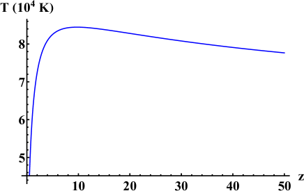
Figure 1: Electron temperatures vs equilibrium fugacity $z=e^{\beta\mu_{(0)}}$. The electron temperature satisfying weak coupling parameter $g<1$ lies above the curve.

Similarly the universal electron thermal velocity is defined $v_{T}\equiv\sqrt{2\langle K\rangle/m_{e}}$ and obtained in equilibrium as follows,

$$v_{T}=\left(\frac{3}{\beta m_{e}}\frac{\mathrm{Li}_{5/2}(-e^{\beta\mu_{(0)}})}{\mathrm{Li}_{3/2}(-e^{\beta\mu_{(0)}})}\right)^{1/2}\,.$$ (19)

Its limiting cases in dilute case, we have $v_{T}\approx\sqrt{3\kappa_{B}T/m_{e}}$ and in dense plasma case $v_{T}\approx\sqrt{(6/5)\,\varepsilon_{F}/m_{e}}$. The ion crystallization  effects (Shukla and Eliasson 2011; Misra and Shukla 2012) for nondegenerate ions that appear due to viscoelasticity of the ions fluid in the momentum equation and cause damping of the ion-acoustic wave are ignored in the model.

II.2 Linear Wave Analysis

II.2.1 Fluid Description

In order to obtain the dispersion relation of IAW in arbitrary degenerate electron plasmas, we linearize the set of dynamic equations (1)-(15) by assuming the perturbations up to first order and the dependent variables are described as follows,

$$n_{i}=n_{0}+n_{i1}\,,\quad n_{e}=n_{0}+n_{e1}\,,\quad v_{i}=v_{i1}\,,\quad\phi=\phi_{1}\,,\quad\mu=\mu_{(0)}+\mu_{1}\,.$$ (20)

The expansion of the polylogarithm function up to to first order is given by

$$\mathrm{Li}_{\nu}(-e^{\beta(\mu_{(0)}+\mu_{1})})=\mathrm{Li}_{\nu}(-e^{\beta\mu_{(0)}})+\beta\mu_{1}\mathrm{Li}_{\nu-1}(-e^{\beta\mu_{(0)}})\text{ }.$$ (21)

The dispersion relation for IAW is obtained by assuming plane wave perturbations $\sim\exp[i(kx-\omega t)]$ i.e.,

$$\omega^{2}=\frac{\omega_{pi}^{2}c_{s}^{2}k^{2}\left(1+\frac{\alpha\,\hslash^{2}k^{2}}{12\,m_{e}m_{i}c_{s}^{2}}\right)}{\omega_{pi}^{2}+\left(1+\frac{\alpha\,\hslash^{2}k^{2}}{12\,m_{e}m_{i}c_{s}^{2}}\right)c_{s}^{2}k^{2}}\,,$$ (22)

where a generalized ion-acoustic speed $c_{s}$ is defined as

$$c_{s}=\sqrt{\frac{1}{m_{i}}\left(\frac{dp}{dn_{e}}\right)_{0}}=\sqrt{\frac{1}{\beta m_{i}}\frac{\mathrm{Li}_{3/2}(-e^{\beta\mu_{(0)}})}{\mathrm{Li}_{1/2}(-e^{\beta\mu_{(0)}})}}$$ (23)

and $\omega_{pi}=\sqrt{n_{0}e^{2}/(m_{i}\varepsilon_{0})}$ is the ion plasma frequency. Here $\left(dp/dn_{e}\right)_{0}$ is evaluated at equilibrium. The limiting cases of ion-acoustic speed i.e., in a dilute plasma (or small fugacity $e^{\beta\mu_{(0)}}\ll 1$) $c_{s}\approx c_{sc}=\sqrt{\kappa_{B}T/m_{i}}$ is obtained, while in dense plasma case (or fugacity $e^{\beta\mu_{(0)}}\gg 1$) we have $c_{s}=\sqrt{(2/3)\varepsilon_{F}/m_{i}}$ and it is the same as obtained by (Maafa 1993) for 3D dense plasmas.

In the long wavelength limit $\alpha\,\hslash^{2}k^{4}/(12m_{e}m_{i})\ll c_{s}^{2}k^{2}\ll\omega_{pi}^{2}$ the dispersion relation (22) IAW gives $\omega^{2}\approx c_{s}^{2}k^{2}$. However, in short wavelength limit the dispersion relation just gives an ion oscillations i.e., $\omega=\omega_{pi}$ and ions are no more shielded by electrons. It happens when the wavelength becomes comparable or shorter than the electron Debye shielding length. It can be seen from Eq. (23) that with the increase in fugacity $e^{\beta\mu_{(0)}}$ (or increase in plasma density) ion-acoustic speed is also increased. It is interesting to note that taking the square root of both sides of Eq. (22) is identical to Eq. (4.5) of Ref. (Eliasson and Shukla, 2010) for completely degenerate plasma case, i.e., $\alpha=1/3$.

II.2.2 Kinetic Description

In section, the dispersion relation for IAW will be obtained using kinetic theory (quantum kinetic) and compare the results already obtained from fluid model and to set value of numerical coefficient $\alpha$ defined in front of the quantum force term in the momentum equation of degenerate electrons. The linear dispersion relation obtained by (Haas 2011) for a Wigner-Poisson system having cold ion and electron species is given by

$$1=\frac{\omega_{pi}^{2}}{\omega^{2}}+\frac{\omega_{pe}^{2}}{n_{0}}\int\frac{f_{0}(\mathbf{v})\,d^{3}v}{(\omega-\mathbf{k}\cdot\mathbf{v})^{2}-\hslash^{2}k^{4}/(4m_{e}^{2})}\,,$$ (24)

where $f_{0}(\mathbf{v})$ is the equilibrium electronic Wigner function and $\omega_{pe}=\sqrt{n_{0}e^{2}/(m_{e}\varepsilon_{0})}$ is the electron plasma frequency.

Now using the 3D Fermi-Dirac distribution of electrons in equilibrium,

$$f_{0}(\mathbf{v})=\frac{\mathcal{A}}{1+e^{\beta(\varepsilon-\mu_{(0)})}},$$ (25)

the longitudinal response of an electron-ion plasma including the first order correction from quantum recoil calculated by (Melrose and Mushtaq 2010),

$$1=\frac{\omega_{pi}^{2}}{\omega^{2}}-\frac{\omega_{pi}^{2}}{c_{s}^{2}k^{2}}\left\{1-\frac{m_{e}\left(\omega^{2}+\hbar^{2}k^{4}/(12\,m_{e}^{2})\right)}{k^{2}\kappa_{B}T}\,\frac{\mathrm{Li}_{-1/2}(-e^{\beta\mu_{(0)}})}{\mathrm{Li}_{1/2}(-e^{\beta\mu_{(0)}})}\right\}$$ (26)

where $\mathcal{A}$ and $\mu_{(0)}$ are related from Eq. (6) in equilibrium. Equation (26) follows the Eq.(29) of (Melrose and Mushtaq 2010) but in different notations. The ionic and electronic responses of plasma appears in the first and second terms on the right-hand side of Eq.(26).

For a low frequency IAW, the static electronic response is taken by putting $\omega\approx 0$ in the last term of Eq. (26), which reduces to

$$1=\frac{\omega_{pi}^{2}}{\omega^{2}}-\frac{\omega_{pi}^{2}}{c_{s}^{2}k^{2}}\left[1-\frac{\hbar^{2}k^{2}}{12\,m_{e}\kappa_{B}T}\,\frac{\mathrm{Li}_{-1/2}(-e^{\beta\mu_{(0)}})}{\mathrm{Li}_{1/2}(-e^{\beta\mu_{(0)}})}\right]\text{ }.$$ (27)

Now solving for wave frequency it gives

$$\omega^{2}=\frac{\omega_{pi}^{2}c_{s}^{2}k^{2}}{\omega_{pi}^{2}+\left[1-\frac{\beta^{2}\hbar^{2}\omega_{pe}^{2}}{12}\,\frac{\mathrm{Li}_{-1/2}(-e^{\beta\mu_{(0)}})}{\mathrm{Li}_{3/2}(-e^{\beta\mu_{(0)}})}\right]c_{s}^{2}k^{2}}.$$ (28)

The dispersion relation obtained from kinetic theory is valid for wavelengths larger than the electron shielding length of the system. Therefore, in order to have comparison with the fluid theory, the dispersion relation of IAW from (28) is expanded for large wavelengths (or small wave numbers), which gives

$$\omega^{2}=c_{s}^{2}k^{2}\left[1+\left\{-1+\frac{\beta^{2}\hbar^{2}\omega_{pe}^{2}}{12}\frac{\mathrm{Li}_{-1/2}(-e^{\beta\mu_{(0)}})}{\mathrm{Li}_{3/2}(-e^{\beta\mu_{(0)}})}\right\}\frac{c_{s}^{2}k^{2}}{\omega_{pi}^{2}}\right]+O(k^{6}).$$ (29)

Also expanding the dispersion relation (22) obtained from fluid theory under large wavelengths, we have

$$\omega^{2}=c_{s}^{2}k^{2}\left[1+\left\{-1+\frac{\alpha\hbar^{2}\omega_{pi}^{2}}{12m_{e}m_{i}c_{s}^{2}}\right\}\frac{c_{s}^{2}k^{2}}{\omega_{pi}^{2}}\right]+O(k^{6}).$$ (30)

The obtained dispersion relations from Eqs. (29) and (30) are equivalent only if, we set

$$\alpha=\frac{\mathrm{Li}_{3/2}(-e^{\beta\mu_{(0)}})\mathrm{Li}_{-1/2}(-e^{\beta\mu_{(0)}})}{\left[\mathrm{Li}_{1/2}(-e^{\beta\mu_{(0)}})\right]^{2}}.$$ (31)

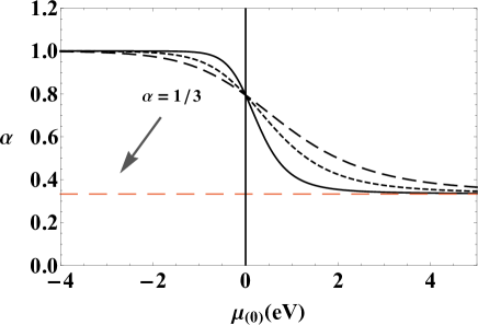
Figure 2: Coefficient $\alpha$ from Eq. (31), as a function of the equilibrium chemical potential $\mu_{(0)}$ is shown at different electron temperatures i.e., $T=4000\,\mathrm{K}$ (solid line), $T=6000\,\mathrm{K}$ (doted line) and $T=8000\,\mathrm{K}$ (dashed line).

It comes out that the numerical coefficient $\alpha$ in the quantum force term in the electron momentum equation has to be function of fugacity $\exp(\beta\mu_{(0)})$ in order to have same dispersion relation from kinetic theory on a quantum ion-acoustic waves in a 3D Fermi-Dirac equilibrium electrons. Now if fugacity $z=\exp(\beta\mu_{(0)})$, then chemical potential in equilibrium $\mu_{(0)}$ can vary from $-\infty$ (classical) to $+\infty$ (dense) plasmas for which $z$ varies from $0$ (dilute) to $\infty$ (ultra-dense) plasmas. Equation (31) gives $\alpha\rightarrow 1$ for $z\rightarrow 0$ case, while $\alpha\rightarrow 1/3$ for $z\rightarrow\infty$. Our limiting case result $\alpha\rightarrow 1$ agrees for nondegenerate plasma case with quantum hydrodynamic model for semi-conductor devices derived in (Gardner 1994), while $\alpha\rightarrow 1/3$ agrees with Refs. (Michta et al. 2015; Akbari-Moghanjoughi 2015) in the fully degenerate case. The behavior of the coefficient $\alpha$ as a function of equilibrium chemical potential ($\mu_{(0)}$) at different temperatures from classical to dense plasma regime is depicted in Fig.2. It is found that slope of the curve in the transition region is found to be decreased with the increase in the temperature of the system. However, the high frequency quantum Langmuir waves are defined for $\alpha=3$ in order to reproduce the Bohm-Pines dispersion relation in Ref. (Bohm and Pines 1953).

II.3 Derivation of Korteweg-de Vries Equation for Ion-acoustic Solitons

After performing the linear analysis of quantum ion-acoustic waves in dense plasma with arbitrary degeneracy of electrons, the above hydrodynamic model will be considered to find out single pulse nonlinear structures such as solitons.

In order to derive the KdV equation for quantum ion-acoustic waves in arbitrary degenerate electron plasmas, the set of dynamic equations (1)-(4), can be written in the normalized form as follows,

$$\frac{\partial\tilde{n}_{i}}{\partial\tilde{t}}+\frac{\partial}{\partial\tilde{x}}(\tilde{n}_{i}\tilde{u}_{i})=0,$$ (32)

$$\frac{\partial\tilde{u}_{i}}{\partial\tilde{t}}+\tilde{u}_{i}\frac{\partial}{\partial\tilde{x}}\tilde{u}_{i}=-\frac{\partial\Phi}{\partial\tilde{x}},$$ (33)

$$0=\frac{\partial\Phi}{\partial\tilde{x}}-\frac{\mathrm{Li}_{1/2}(-e^{\beta\mu_{(0)}})}{\mathrm{Li}_{1/2}(-e^{\beta\mu})}\frac{\partial\tilde{n}_{e}}{\partial\tilde{x}}+\frac{H^{2}}{2}\frac{\partial}{\partial\tilde{x}}\left(\frac{1}{\sqrt{\tilde{n}_{e}}}\frac{\partial^{2}}{\partial\tilde{x}^{2}}\sqrt{\tilde{n}_{e}}\right),$$ (34)

$$\frac{\partial^{2}\Phi}{\partial\tilde{x}^{2}}=\tilde{n}_{e}-\tilde{n}_{i},$$ (35)

where a dimensionless quantum diffraction parameter $H$ is

$$H=\frac{\beta\hbar\omega_{{}_{pe}}}{\sqrt{3}}\left[\frac{\mathrm{Li}_{-1/2}(-e^{\beta\mu_{(0)}})}{\mathrm{Li}_{3/2}(-e^{\beta\mu_{(0)}})}\right]^{1/2}.$$ (36)

The limiting case of quantum diffraction parameter  for a dilute plasma comes out to be $H\approx\beta\hbar\omega_{{}_{pe}}/\sqrt{3}$, while in case of a fully degenerate plasma $H\approx\hbar\omega_{{}_{pe}}/(2\varepsilon_{F})$, respectively. Also, equation (13) in normalized form gives,

$$\tilde{n}_{e}=\frac{\mathrm{Li}_{3/2}(-e^{\beta\mu})}{\mathrm{Li}_{3/2}(-e^{\beta\mu_{(0)}})}.$$ (37)

The normalization of space, time, ion fluid velocity and electrostatic potential i.e., $\tilde{x}\rightarrow\omega_{{}_{pi}}x/c_{s}$, $\tilde{t}\rightarrow t\omega_{{}_{pi}}$, $\tilde{u}_{i}\rightarrow u_{i}/c_{s}$ and $\Phi=e\phi/m_{i}c_{s}^{2}$, respectively, has been defined. Here $c_{s}$ is the ion-acoustic speed defined in equation (23). The normalization of electron and ion fluid density is defined as $\tilde{n}_{j}=n_{j}/n_{0}$ ($j=e,i$). In further calculations, for simplicity we will not use the tilde sign on normalized quantities.

In order to find the KdV equation, the stretching of the independent variables $x$, $t$ is defined as follows (Haas et al. 2003; Mahmood and Haas 2014),

$$\xi=\varepsilon^{1/2}(x-V_{0}t)\,,\quad\tau=\varepsilon^{3/2}t,$$

where $\varepsilon$ is a small expansion parameter and $V_{0}$ is the phase velocity of the wave to be determined later on. The perturbed quantities can be expanded in the orders of small expansion parameter as follows,

$$n_{j1}=1+\varepsilon n_{j1}+\varepsilon^{2}n_{j2}+...,\text{ (here }j=e,i\text{)}$$

$$u_{i}=\varepsilon u_{i1}+\varepsilon^{2}u_{i2}+...,$$

$$\Phi=\varepsilon\Phi_{1}+\varepsilon^{2}\Phi_{2}+...,$$

$$\mu=\mu_{(0)}+\varepsilon\mu_{1}+\varepsilon^{2}\mu_{2}+...$$ (38)

Now collecting lowest order set of dynamic equations and after solving them, we get

$$V_{0}=\pm 1$$ (39)

which is the normalized phase velocity of the wave. Further more, we set $V_{0}=1$ without loss of generality. Using above relation (39), the first order perturbed quantities are related as

$$n_{i1}=u_{i1}=n_{e1}=\Phi_{1}.$$ (40)

The next higher order perturbation terms of the set of dynamic equations are given by

$$\frac{\partial n_{i2}}{\partial\xi}=\frac{\partial n_{i1}}{\partial\tau}+\frac{\partial}{\partial\xi}(n_{i1}u_{i1})+\frac{\partial u_{i1}}{\partial\tau}+u_{i1}\frac{\partial u_{i1}}{\partial\xi}+\frac{\partial\Phi_{2}}{\partial\xi},$$ (41)

$$\frac{\partial n_{e2}}{\partial\xi}=\frac{\partial\Phi_{2}}{\partial\xi}+\alpha n_{e1}\frac{\partial n_{e1}}{\partial\xi}+\frac{H^{2}}{4}\frac{\partial^{3}n_{e1}}{\partial\xi^{3}}.$$ (42)

On solving the next higher order Poisson’s equation together with Eqs. (39), (41) and (42), the obtained KdV equation for quantum ion-acoustic waves in plasmas with arbitrary degeneracy of electrons  in terms of $\Phi_{1}$ is given by,

$$\frac{\partial\Phi_{1}}{\partial\tau}+a\Phi_{1}\frac{\partial\Phi_{1}}{\partial\xi}+b\frac{\partial^{3}\Phi_{1}}{\partial\xi^{3}}=0,$$ (43)

where the nonlinear and dispersive coefficients $a$ and $b$ i.e.,

$$a=\frac{3-\alpha}{2},$$ (44)

$$b=\frac{1}{2}\left(1-\frac{H^{2}}{4}\right),$$ (45)

are defined. The limiting case of dilute (classical) plasma for nonlinear and dispersive coefficients gives $a=1$ and $b=1/2$ respectively in the absence of Bohm potential, which are same as already derived in Ref. (Davidson 1972) for the KdV equation in a low density classical plasma. Both nonlinear and dispersive coefficients have arbitrary degeneracy electrons effects appearing in $\alpha$ and quantum parameter $H$ respectively.

The traveling wave solution of the KdV equation (43) in terms of single pulse soliton is given by

$$\Phi_{1}=D\,\mathrm{sech}^{2}(\eta/W),$$ (46)

where $D=3u_{0}/a$ and $W=\sqrt{4b/u_{0}}$ are the amplitude and width of the soliton, respectively. Also $\eta=\xi-u_{0}\tau$ is the transformed coordinate in the comoving frame and $u_{0}$ is the speed of the soliton. The potential hump or dip structure of the quantum IAW soliton depends on the sign of $D$. The decaying boundary condition have been used for soliton structure. Now using the relation of stretched coordinates $(\xi,\tau)$ the transformed coordinate $\eta$ can be described as $\eta=\varepsilon^{1/2}\tilde{\eta}$ where $\tilde{\eta}=x-Vt$ and $V=V_{0}+\varepsilon u_{0}$ is the soliton velocity in the laboratory frame. The dispersive coefficient described in Eq.(43) vanishes at $H=2$ and shock formation occurs in the absence of dispersive effects in the system. In that case, the dispersive effects can be included through higher order perturbation theory and Kawahara equation is obtained (Kawahara 1972). The quantum ion-acoustic soliton solution exist only if $H\neq 2$ and dispersive coefficient does not disappear. The nonlinear coefficient $a$ will always come out to be positive because the numerical value of parameter $\alpha$ varies from $1$ to $1/3$ from dilute to dense plasma case. A proper balance between the nonlinearity and dispersion in the system gives a soliton structure.

Figure 3: (a): Electrostatic potential hump ion-acoustic soliton structure (moving with supersonic speed in lab frame) is shown from Eq. (46) for $H<2$  case with $\alpha=0.5,$ $H=0.5,$ $\varepsilon=0.1$ and $u_{0}=0.1$. (b): Electrostatic potential dip ion-acoustic soliton structure (moving with subsonic speed in lab frame) is shown from Eq. (46) for $H>2$ case with $\alpha=0.5,$ $H=2.05,$ $\varepsilon=0.1$ and $u_{0}=-0.1$.

In case if $H<2$, then $u_{0}$ must have positive values to give the real value of soliton width $W$ for which $D>0$ holds and potential hump (bright) soliton structure is obtained which moves with super-sonic speed in the forward direction as $V>V_{0}$ . However, when $H>2$, then $u_{0}$ must have negative values to give the real value of soliton width $W$ for which $D<0$ holds and potential dip (dark) soliton structure is obtained which moves with sub-sonic speed in the backward direction as $V<V_{0}$ (Belashov and Vladimirov 2005). Therefore, the formation of both potential hump (bright) and dip (dark) quantum ion-acoustic soliton are possible in our present model. The numerical presentation of the bright ($H<2$) and dark ($H>2$) quantum ion-acoustic solitons obtained from Eq. (46) are shown in Figs. 3a and 3b, respectively. The quantum ion-acoustic potential hump (bright) soliton structure is obtained for $z=5$, $T=10^{5}$K , which corresponds to plasma density $n_{0}=3.3\times 10^{29}$ $\mathrm{m}^{-3}$ , while quantum diffraction parameter and electron plasma frequency comes out to be $H=0.64$, $\omega_{pe}=3.3\times 10^{16}\,$$\mathrm{rad/s}$, respectively. However, quantum ion-acoustic potential dip (dark) soliton structure is obtained for $z=5$, $T=10^{3}$K , which corresponds to plasma density $n_{0}=3.5\times 10^{26}$ $\mathrm{m}^{-3}$ , while quantum diffraction parameter and electron plasma frequency comes out to be $H=2.03$ and $\omega_{pe}=1.1\times 10^{15}\,$$\mathrm{rad/s}$, respectively. It can be seen from Eqs.(44) and (45) that for large values of nonlinear and dispersive coefficients $a$ and $b$ (or in a more dense plasma) the small amplitude and large width soliton structures are formed. This happens because under assumption of strong degeneracy, it becomes difficult to accommodate more Fermions in a localized structure or wave packet.

II.3.1 Conditions for the existence of bright and dark quantum ion-acoustic solitons

In this step, we will look for the physical condition for the propagation of bright and dark IAW soliton i.e., for $H<2$ or $H>2$ respectively, in a quantum plasma. Now using the relation (8) of plasma equilibrium density the dimensionless quantum parameter from Eq. (36) can be written as

$$H^{2}=-\frac{1}{3\pi}\left(\frac{m_{e}}{2\,\pi\kappa_{B}T}\right)^{1/2}\frac{e^{2}}{\hbar\varepsilon_{0}}\mathrm{Li}_{-1/2}(-e^{\beta\mu_{(0)}}).$$ (47)

From above equation, the condition for the system temperature at which$H>2$ occurs can be found out as follows

$$\kappa_{B}T<\frac{m_{e}}{288\,\pi^{3}}\left(\frac{e^{2}}{\hbar\varepsilon_{0}}\right)^{2}\left[\mathrm{Li}_{-1/2}(-e^{\beta\mu_{(0)}})\right]^{2}\text{.}$$ (48)

Similarly under the weak coupling condition for an ideal Fermi gas, the upper bound on quantum diffraction parameter $H$ can be found by using the minimal temperature in Eq. (18) with Eq. (47), which gives

$$H^{2}<H_{M}^{2}=\left(\frac{3}{\pi}\right)^{1/3}\frac{\mathrm{Li}_{-1/2}(-e^{\beta\mu_{(0)}})\mathrm{Li}_{5/2}(-e^{\beta\mu_{(0)}})}{\left[\mathrm{Li}_{3/2}^{2}(-e^{\beta\mu_{(0)}})\right]^{2/3}}.$$ (49)

It can be seen numerically that large $H>2$ values fall within the the strongly coupled regime where the coupling parameter $g$ defined in Eq. (17) may become near or greater than one.

III Ion-acoustic Waves for Magnetized Quantum Plasmas with Arbitrary Degeneracy of Electrons

In this section, we will investigate the quantum IAW in a magnetized plasma with arbitrary degeneracy of electrons. The external magnetic field is assumed to be directed along x-axis i.e., $\mathbf{B}_{0}=B_{0}\hat{x}$ and the obliquely propagating electrostatic wave lies in the XY plane i.e., $\mathbf{\nabla}=(\partial_{x},\partial_{y},0)$. The ions are considered to be inertial, while electron quantum fluid is assumed to be inertialess. The material in this section is a review based on (Haas and Mahmood 2016). The set of dynamic equations with arbitrary degeneracy of electrons in a magnetized dense plasma are given below.

The ion continuity and momentum equations are described as follow:

$$\frac{\partial n_{i}}{\partial t}+\frac{\partial}{\partial x}(n_{i}u_{ix})+\frac{\partial}{\partial y}(n_{i}u_{iy})=0\,,$$ (50)

$$\frac{\partial u_{ix}}{\partial t}+\left(u_{ix}\frac{\partial}{\partial x}+u_{iy}\frac{\partial}{\partial y}\right)u_{ix} =-\frac{e}{m_{i}}\frac{\partial\phi}{\partial x}\,,$$ (51)

$$\frac{\partial u_{iy}}{\partial t}+\left(u_{ix}\frac{\partial}{\partial x}+u_{iy}\frac{\partial}{\partial y}\right)u_{iy} =-\frac{e}{m_{i}}\frac{\partial\phi}{\partial y}+\omega_{ci}u_{iz}\,,$$ (52)

$$\frac{\partial u_{iz}}{\partial t}+\left(u_{ix}\frac{\partial}{\partial x}+u_{iy}\frac{\partial}{\partial y}\right)u_{iz} =-\omega_{ci}u_{iy}\,.$$ (53)

The momentum equation for the inertialess degenerate electrons is

$$0=-\frac{\nabla p}{n_{e}}+e\nabla\phi+\frac{\alpha\hbar^{2}}{6m_{e}}\nabla\left[\frac{1}{\sqrt{n_{e}}}\left(\frac{\partial^{2}}{\partial x^{2}}+\frac{\partial^{2}}{\partial y^{2}}\right)\sqrt{n_{e}}\right]\,.$$ (54)

The Poisson equation is given by

$$\left(\frac{\partial^{2}}{\partial x^{2}}+\frac{\partial^{2}}{\partial y^{2}}\right)\phi=\frac{e}{\varepsilon_{0}}(n_{e}-n_{i}),$$ (55)

here $\phi$ is the electrostatic potential. The electron and ion fluid densities are represented by $n_{e}$ and $n_{i}$ respectively while $\mathbf{u}_{i}=(u_{ix},u_{iy},u_{iz})$ is the ion fluid velocity and its components along $x$, $y$ and $z$ directions. The electron and ion masses are represented by $m_{e}$ and $m_{i}$ respectively, while $-e$ is the electronic charge, $\varepsilon_{0}$ is the vacuum permittivity, $\hbar$ is the reduced Planck constant. The ion cyclotron frequency is$\ \omega_{ci}=eB_{0}/m_{i}$ . The electron’s fluid pressure $p=p(n_{e})$ is specified by a barotropic equation of state (10) obtained from the moments of a local Fermi-Dirac distribution function of an ideal Fermi gas. The last term on the right hand side of the momentum equation (54) for electrons is the quantum force, which arises from the Bohm potential, giving rise to quantum diffraction or tunneling effects due to the wave like nature of the charged particles. The equilibrium is defined as $n_{e0}=n_{i0}\equiv n_{0}$. The numerical factor $\alpha$ is defined in the quantum force term of Eq. (54) in order to fit the kinetic linear dispersion relation in the long wavelength limit, in a 3D Fermi-Dirac equilibrium. The mathematical expression of numerical coefficient $\alpha$ in terms of polylogarithm function $\mathrm{Li}$ with fugacity dependence has been derived in Eq. (31) from finite-temperature quantum kinetic theory for low frequency IAW excitations. Furthermore, the electron density $n_{e}$ and chemical potential $\mu$ are related through relation (13) in a quasi-Fermi Dirac equilibrium, while electron equilibrium chemical potential $\mu_{0}$ is related to the equilibrium density $n_{0}$ through relation (8), respectively.

III.1 Linear Wave Analysis

III.1.1 Fluid Description

The dispersion relation of electrostatic waves in a magnetized dense plasma with arbitrary degeneracy of electrons will be discussed in this section. In order to find the dispersion relation, the set of dynamic ion and electron fluid equations (50)-(55) are linearized up to first order by defining the dependent variables as follows:

$$n_{i}=n_{0}+n_{i1}\,,n_{e}=n_{0}+n_{e1}\,,u_{ix}=u_{ix1}\,,u_{iy}=u_{iy1}\,,u_{iz}=u_{iz1}\,,\phi=\phi_{1}\,\text{and }\mu=\mu_{(0)}+\mu_{1}.$$ (56)

By assuming the plane wave perturbations $\sim\exp[i(k_{x}x+k_{y}y-\omega t)]$, the obtained dispersion relation of electrostatic waves in a magnetized quantum plasma is

$$1+\chi_{i}(\omega,\mathbf{k})+\chi_{e}(0,\mathbf{k})=0\,,$$ (57)

where the ionic and electronic susceptibilities are described by

$$\chi_{i}(\omega,\mathbf{k}) =-\,\frac{\omega_{pi}^{2}(\omega^{2}-\omega_{ci}^{2}\cos^{2}\theta)}{\omega^{2}(\omega^{2}-\omega_{ci}^{2})}\,,$$ (58)

$$\chi_{e}(0,\mathbf{k}) =\omega_{pe}^{2}\left[\frac{1}{m_{e}}\left(\frac{dp}{dn_{e}}\right)_{0}k^{2}+\frac{\alpha\hbar^{2}k^{4}}{12m_{e}^{2}}\right]^{-1}\!\!\!,$$ (59)

where $\omega_{pj}^{2}=n_{0}e^{2}/(m_{j}\varepsilon_{0})$ for $j=i,e$ and $\mathbf{k}=k\,(\cos\theta,\sin\theta,0)$. Here $\chi_{e}(0,\mathbf{k})$ is the static electronic susceptibility due to inertialess electron quantum fluid. There is no loss of generality in assuming waves propagation in the XY plane, due to symmetry around the direction of the external magnetic field i.e., $x$-axis.

The dispersion relation (57) along with Eqs.(58) and (59) gives a quadratic equation for $\omega^{2}$ and its obtained solution is given by

$$\omega^{2}=\frac{1}{2}\left[\omega_{0}^{2}+\omega_{ci}^{2}\pm\left\{(\omega_{0}^{2}+\omega_{ci}^{2})^{2}-4\omega_{0}^{2}\omega_{ci}^{2}\cos^{2}\theta\right\}^{1/2}\right]\,,$$ (60)

and

$$\omega_{0}^{2}=\frac{c_{s}^{2}k^{2}\left[1+H^{2}(k\lambda_{D})^{2}/4\right]}{1+(k\lambda_{D})^{2}+H^{2}(k\lambda_{D})^{4}/4}\,,$$ (61)

where $\omega_{0}$ is the wave frequency of quantum IAW in unmagnetized plasma derived in Eq.(22), $c_{s}$ is the ion-acoustic speed and $H$ is the quantum diffraction parameters defined in Eqs. (23) and (36) respectively. Also the generalized screening length of degenerate electrons is defined as

$$\lambda_{D}^{2}=\frac{c_{s}^{2}}{\omega_{pi}^{2}}=\frac{\kappa_{B}T}{m_{e}\omega_{pe}^{2}}\,\frac{\mathrm{Li}_{3/2}(-e^{\beta\mu_{(0)}})}{\mathrm{Li}_{1/2}(-e^{\beta\mu_{(0)}})}\,.$$ (62)

In a low fugacity $e^{\beta\mu_{(0)}}\ll 1$ or dilute plasma case, the ion-acoustic speed and electron Debye length becomes $c_{s}\approx\sqrt{\kappa_{B}T/m_{i}},\,\lambda_{D}=\sqrt{\kappa_{B}T/(m_{e}\omega_{pe}^{2})}$, respectively, which are same as in classical plasma. The quantum diffraction parameter in dilute plasma case is $H\approx\beta\hbar\omega_{pe}/\sqrt{3}$. However in fully degenerate or dense plasma case i.e., for fugacity $e^{\beta\mu_{(0)}}\gg 1$, the quantum ion-acoustic speed and Thomas-Fermi screening length comes out to be $c_{s}\approx\sqrt{(2/3)\varepsilon_{F}/m_{i}},\,\lambda_{D}=\sqrt{2\varepsilon_{F}/(3m_{e}\omega_{pe}^{2})}$ and quantum diffraction parameter is $H\approx(1/2)\hbar\omega_{pe}/\varepsilon_{F}$ where $\mu_{(0)}\approx\varepsilon_{F}=\hbar^{2}(3\pi^{2}n_{0})^{2/3}/(2m_{e})$ is the Fermi energy. The obtained dispersion relation (60) of electrostatic waves in a magnetized quantum plasma with arbitrary degeneracy of electrons gives the same dispersion relation for classical magnetized plasma (Stringer 1963; Witt and Lotko 1983) in the limiting case of dilute plasmas.

The two symmetrical roots with “positive” and “negative” signs of Eq. (60) corresponds to the fast (ion cyclotron branch) and slow (ion-acoustic branch) electrostatic waves, respectively, in a magnetized quantum plasma because electrons stream along the magnetic field lines to neutralize the ions   [Bernhardt et al., 2009]. For almost perpendicular wave propagation to the magnetic field, there exist also the lower hybrid wave (LHW) which involves the electron inertia via polarization drift and it is out of scope to our present research work. The dependence of arbitrary degeneracy of electrons for arbitrary wave propagation angle $\theta$ is not clearly evident from Eq. (60) due to its complexity. However, in the presence of strong quantum effects $\omega_{0}^{2}\gg\omega_{ci}^{2}$, the fast mode gives $\omega^{2}\approx\omega_{0}^{2}+\omega_{ci}^{2}\sin^{2}\theta$ and slow mode becomes $\omega^{2}\approx\omega_{ci}^{2}\cos^{2}\theta$. It means the fast electrostatic wave frequency has angular dependence as well as quantum correction, while the slow electrostatic wave frequency is only angle dependent and it is not influenced by quantum effects. In order to have validity of our model, we consider the example solid density hydrogen laboratory plasma parameters $T=10^{6}\,\mathrm{K},\,n_{0}=5\times 10^{30}\,\mathrm{m}^{-3}$ in ambient magnetic field $B_{0}=10^{3}\,\mathrm{T}$ and wave-number $k=2\pi\times 10^{9}\,\mathrm{m}^{-1}$, which gives the ion cyclotron frequency $\omega_{ci}=9.58\times 10^{10}\,\mathrm{rad/s}$ and $\omega_{0}=6.50\times 10^{14}\,\mathrm{rad/s}\gg\omega_{ci}$.

Some significant limiting cases of Eq. (60) are described below:

1. Wave propagation in the parallel direction to the magnetic field: In case of wave propagation in the parallel direction to the magnetic field i.e., $\theta=0$ then two symmetrical roots of the Eq. (60) are $\omega=\omega_{ci}$ (ion cyclotron frequency) and $\omega=\omega_{0}$. Therefore one root $\omega=\omega_{ci}$ pure oscillating mode while the other root $\omega=\omega_{0}$ becomes the ion acoustic wave propagation mode i.e., $\omega_{0}\approx c_{s}k$ in the long wavelength limit $k\lambda_{D}\ll 1$. The quantum degeneracy effects appear only in the ion acoustic wave mode.

2. Wave propagation in the perpendicular direction to the magnetic field: In case of exact perpendicular wave propagation i.e., $\theta=\pi/2$, the two symmetrical roots of Eq. (60) come out to be $\omega=0$ (mode vanishes) and $\omega=\left(\omega_{ci}^{2}+\omega_{0}^{2}\right)^{1/2}$. The ion cyclotron mode is modified in the quantum effects in a magnetized plasma.

3. Strongly magnetized ions case: In case of a strongly magnetized ions plasma i.e., $\omega_{ci}\gg\omega_{0}$, then from Eq.(60) we have for the fast mode

$$\omega^{2}=\omega_{ci}^{2}\left[1+\frac{\omega_{0}^{2}}{\omega_{ci}^{2}}\sin^{2}\theta+\frac{\omega_{0}^{4}}{4\,\omega_{ci}^{4}}\sin^{2}(2\theta)+\mathcal{O}\left(\left(\frac{\omega_{0}}{\omega_{ci}}\right)^{6}\right)\right]\,,$$ (63)

while the slow mode becomes

$$\omega^{2}=\omega_{0}^{2}\cos^{2}\theta\left[1-\frac{\omega_{0}^{2}}{\omega_{ci}^{2}}\sin^{2}\theta+\mathcal{O}\left(\left(\frac{\omega_{0}}{\omega_{ci}}\right)^{4}\right)\right]\,.$$ (64)

III.1.2 Kinetic Description

The dispersion relation (60) obtained from fluid description must agrees with the results of kinetic theory in the long wavelength limit. Therefore, ionic and electronic susceptibilities obtained from kinetic theory must be compared with Eqs. (58) and (59) obtained from fluid dynamics. In order to find the ionic response, the particle distribution of classical ions $f_{i}=f_{i}(\mathbf{r},\mathbf{v},t)$ satisfy the Vlasov’s equation as follows

$$\left[\frac{\partial}{\partial t}+\mathbf{v}\cdot\nabla+\frac{e}{m_{i}}(-\nabla\phi+\mathbf{v}\times\mathbf{B}_{0})\cdot\frac{\partial}{\partial\mathbf{v}}\right]f_{i}=0\,.$$ (65)

Due to quantum nature of electrons, the quantum Vlasov equation is satisfied by the electronic Wigner quasi-distribution $f_{e}=f_{e}(\mathbf{r},\mathbf{v},t)$,

$$\frac{\partial f_{e}}{\partial t} +\mathbf{v}\cdot\nabla f_{e}-\frac{ie}{\hbar}\left(\frac{m_{e}}{2\pi\hbar}\right)^{3}\times\int d\mathbf{s}\,d\mathbf{v}^{\prime}\exp\left(\frac{im_{e}(\mathbf{v}^{\prime}-\mathbf{v})\cdot\mathbf{s}}{\hbar}\right)\times$$

$$\times\left[\phi\left(\mathbf{r}+\frac{\mathbf{s}}{2},t\right)-\phi\left(\mathbf{r}-\frac{\mathbf{s}}{2},t\right)\right]f_{e}(\mathbf{r},\mathbf{v}^{\prime},t)=0\,.$$ (66)

All integrals run from $-\infty$ to $\infty$, unless otherwise stated. Also, the magnetic force effects on electrons are ignored under the assumption of large electron thermal and quantum (statistical and diffraction) effects.

The scalar potential is find out from Poisson’s equation,

$$\left(\frac{\partial^{2}}{\partial x^{2}}+\frac{\partial^{2}}{\partial y^{2}}\right)\phi=\frac{e}{\varepsilon_{0}}\left(\int\!f_{e}\,d\mathbf{v}-\int\!f_{i}\,d\mathbf{v}\right)\,,$$ (67)

where spatial variations are considered in the XY-plane.

The dispersion relation $1+\chi_{i}(\omega,\mathbf{k})+\chi_{e}(\omega,\mathbf{k})=0$ for electrostatic waves in a magnetized quantum plasma is easily obtained by assuming plane wave perturbations $\sim\exp[i(k_{x}x+k_{y}y-\omega t)]$ around isotropic distribution in velocities equilibria. In case of cold ions and ignoring the Landau damping effects the ion susceptibility obtained from kinetic theory (Stepanov 1959; Akhiezer et al. 1975) coincides well with its fluid description (58). However, under the assumption of low frequency waves the static electronic response gives

$$\chi_{e}(0,\mathbf{k})=\frac{e^{2}}{\varepsilon_{0}\hbar k^{2}}\int\!\frac{d\mathbf{v}}{\mathbf{k}\cdot\mathbf{v}}\!\left[F\left(\mathbf{v}\!-\!\frac{\hbar\mathbf{k}}{2m_{e}}\right)-F\left(\mathbf{v}\!+\!\frac{\hbar\mathbf{k}}{2m_{e}}\right)\right],$$ (68)

where the principal value of the integral is understood if necessary and where the equilibrium electronic Wigner function is $f_{e}=F(\mathbf{v})$.

Now considering a Fermi-Dirac equilibrium for degenerate electrons,

$$F(\mathbf{v})=\frac{\mathcal{A}}{1+e^{\beta(m_{e}v^{2}/2-\mu_{(0)})}}\,,\quad v=|\mathbf{v}|\,,$$ (69)

where normalization constant $\mathcal{A}$ assuring that $\int\!F(\mathbf{v})\,d\mathbf{v}=n_{0}$.

Now using Eq. (68) in Eq. (68), the static electronic susceptibility $\chi_{e}(0,\mathbf{k})$ can be expressed in the power series of small quantum recoil $q=\sqrt{\beta/(2m_{e})}\,\hbar k/2$ for sufficiently large electron temperature and long wavelength assumption i.e.,

$$\chi_{e}(0,\mathbf{k}) =\frac{\beta m_{e}\omega_{pe}^{2}}{\sqrt{\pi}\,\mathrm{Li}_{3/2}(-z)k^{2}}\left[\Gamma\left(\frac{1}{2}\right)\mathrm{Li}_{1/2}(-z)+\Gamma\left(-\frac{1}{2}\right)\mathrm{Li}_{-1/2}(-z)\frac{q^{2}}{3}\right.$$

$$\left.+\Gamma\left(-\frac{3}{2}\right)\mathrm{Li}_{-3/2}(-z)\frac{q^{4}}{5}+\dots\right]$$

$$=\frac{\beta m_{e}\omega_{pe}^{2}}{\sqrt{\pi}\,\mathrm{Li}_{3/2}(-z)k^{2}}\sum_{j=0}^{\infty}\Gamma\left(\frac{1}{2}-j\right)\times\mathrm{Li}_{1/2-j}(-z)\frac{q^{2j}}{2j+1}\,,$$ (70)

where fugacity is $z=e^{\beta\mu_{(0)}}$. The above expression (70) is exact, as long as the series converges and $\chi_{e}(0,\mathbf{k})$ has the same expression as in Eq. (29) of (Melrose and Mushtaq 2010), where quantum recoil correction of $\mathcal{O}(q^{2})$ was retained.

In order to have a comparison with fluid model results the expression $\chi_{e}(0,\mathbf{k})$ described in Eq.(59) can be re-written in the powers of small quantum recoil correction $q$ as follows,

$$\chi_{e}(0,\mathbf{k}) =\frac{\beta m_{e}\omega_{pe}^{2}\mathrm{Li}_{1/2}(-z)}{\,\mathrm{Li}_{3/2}(-z)k^{2}}\left(1+\frac{2q^{2}}{3}\frac{\mathrm{Li}_{-1/2}(-z)}{\mathrm{Li}_{1/2}(-z)}\right)^{-1}$$

$$=\frac{\beta m_{e}\omega_{pe}^{2}}{\,\mathrm{Li}_{3/2}(-z)k^{2}}\left[\mathrm{Li}_{1/2}(-z)-\frac{2q^{2}}{3}\mathrm{Li}_{-1/2}(-z)+\mathcal{O}(q^{4})\,\right]\text{ ,}$$ (71)

which is the same as described in Eq. (70) in the long wavelength limit, where $\Gamma(1/2)=\sqrt{\pi},\,\,\Gamma(-1/2)=-2\sqrt{\pi}$. It also justifies the inclusion numerical parameter $\alpha$ in the quantum force of Eq. (54) in the magnetized dense plasma case to compare the results of kinetic theory with the fluid description of 3D Fermi-Dirac distributed electrons.

III.2 Zakharov-Kuznetsov (ZK) Equation for Ion-acoustic Waves in a Magnetized Dense Plasma

In this section, we will derive ZK equation for the two dimensional propagating ion-acoustic soliton in a magnetized quantum plasma with arbitrary degeneracy of electrons. The set of dynamic equations (50)-(55) can be written in normalized or dimensionless form as follows,

$$\frac{\partial\tilde{n}_{i}}{\partial\tilde{t}}+\frac{\partial}{\partial\tilde{x}}(\tilde{n}_{i}\tilde{u}_{ix})+\frac{\partial}{\partial\tilde{y}}(\tilde{n}_{i}\tilde{u}_{iy})=0\,,$$ (72)

$$\frac{\partial\tilde{u}_{ix}}{\partial\tilde{t}}+\left(\tilde{u}_{ix}\frac{\partial}{\partial\tilde{x}}+\tilde{u}_{iy}\frac{\partial}{\partial\tilde{y}}\right)\tilde{u}_{ix}=-\frac{\partial\tilde{\phi}}{\partial\tilde{x}}\,,$$ (73)

$$\frac{\partial\tilde{u}_{iy}}{\partial\tilde{t}}+\left(\tilde{u}_{ix}\frac{\partial}{\partial\tilde{x}}+\tilde{u}_{iy}\frac{\partial}{\partial\tilde{y}}\right)\tilde{u}_{iy}=-\frac{\partial\tilde{\phi}}{\partial\tilde{y}}+\Omega\tilde{u}_{iz}\,,$$ (74)

$$\frac{\partial\tilde{u}_{iz}}{\partial\tilde{t}}+\left(\tilde{u}_{ix}\frac{\partial}{\partial\tilde{x}}+\tilde{u}_{iy}\frac{\partial}{\partial\tilde{y}}\right)\tilde{u}_{iz}=-\Omega\tilde{u}_{iy}\,,$$ (75)

$$0=\tilde{\nabla}\tilde{\phi}-\frac{\mathrm{Li}_{1/2}(-e^{\beta\mu_{(0)}})}{\mathrm{Li}_{1/2}(-e^{\beta\mu})}\tilde{\nabla}\tilde{n}_{e}+\frac{H^{2}}{2}\tilde{\nabla}\left[\frac{1}{\sqrt{\tilde{n}_{e}}}\left(\frac{\partial^{2}}{\partial\tilde{x}^{2}}+\frac{\partial^{2}}{\partial\tilde{y}^{2}}\right)\sqrt{\tilde{n}_{e}}\right]$$ (76)

$$\left(\frac{\partial^{2}}{\partial\tilde{x}^{2}}+\frac{\partial^{2}}{\partial\tilde{y}^{2}}\right)\tilde{\phi}=\tilde{n}_{e}-\tilde{n}_{i},$$ (77)

where $\Omega=\omega_{ci}/\omega_{pi}$ and $\tilde{\nabla}=(\partial/\partial\tilde{x},\partial/\partial\tilde{y},0)$ have been defined. The expression of normalized electron density for arbitrary degenerate electrons has already been described in Eq. (37). The normalization of dependent variables $(\tilde{u}_{ix},\tilde{u}_{iy},\tilde{u}_{iz})=(u_{ix},u_{iy},u_{iz})/c_{s}$, $\tilde{\phi}=e\phi/(m_{i}c_{s}^{2})$, $\tilde{n}_{j}=n_{j}/n_{0}$, where $j=e,i$, while for independent variables $(\tilde{x},\tilde{y})=(x,y)/\lambda_{D}$, $\tilde{t}=\omega_{{}_{pi}}t$ has been defined. For simplicity, the tilde sign will be omitted from normalized quantities in further calculations.

In order to find a nonlinear evolution equation for obliquely propagating ion-acoustic wave in a dense magnetized plasma, the stretching of the independent variables ($x,$ $y,$ $t$) is defined under the assumption of strong magnetization as follows (Kourakis et al. 2009; Mace and Hellberg 2001; Infeld 1985; Laedke and Spatschek 1982),

$$X=\varepsilon^{1/2}(x-V_{0}t)\,,\quad Y=\varepsilon^{1/2}y\,,\quad\tau=\varepsilon^{3/2}t\,,$$ (78)

where $\varepsilon$ is a small expansion parameter and $V_{0}$ is the phase velocity of the wave, to be determined later on. The perturbed quantities can be expanded in powers of $\varepsilon$ as follows,

$$n_{j} =1+\varepsilon n_{j1}+\varepsilon^{2}n_{j2}+...\,,\quad j=e,i\,,$$ (79)

$$u_{ix} =\varepsilon u_{x1}+\varepsilon^{2}u_{x2}+\varepsilon^{3}u_{x3}...\,,$$ (80)

$$u_{i\perp} =\varepsilon^{3/2}u_{\perp 1}+\varepsilon^{2}u_{\perp 2}+\varepsilon^{5/2}u_{\perp 3}...\,,\quad\perp=y,z\,,$$ (81)

$$\phi =\varepsilon\phi_{1}+\varepsilon^{2}\phi_{2}+...\,,$$ (82)

$$\mu =\mu_{(0)}+\varepsilon\mu_{1}+\varepsilon^{2}\mu_{2}+...$$ (83)

In the above perturbation scheme, the ion fluid velocity components ($u_{iy}$, $u_{iz}$) in the perpendicular direction of the external magnetic field are taken to be of higher order perturbations in comparison with the ion parallel fluid velocity component $u_{ix}$ because in the presence of magnetic field the anisotropy of fluid velocities occurs and ion gyro-motion becomes a higher order effect.

Now collecting the lowest $\varepsilon$ order terms from the set of dynamic equations (72)-(77) and on solving  them together, we obtain $V_{0}=\pm 1$, which is the normalized phase velocity of the ion-acoustic waves in a magnetized dense plasma. In further calculations, we set $V_{0}=1$ without loss of generality.

Collecting the next higher $\varepsilon$ order terms from the set of dynamic equations (72)-(77), it is finally possible to write the ZK equation for obliquely propagating ion-acoustic wave in a magnetized quantum plasma in terms of $\phi_{1}\equiv\varphi$,

$$\frac{\partial\varphi}{\partial\tau}+A\varphi\frac{\partial\varphi}{\partial X}+\frac{\partial}{\partial X}\left(B\frac{\partial^{2}\varphi}{\partial X^{2}}+C\frac{\partial^{2}\varphi}{\partial Y^{2}}\right)=0\,,$$ (84)

where nonlinearity coefficient $A$ and the dispersion coefficients in the parallel $(B)$ and perpendicular $(C)$ directions of the external magnetic field, respectively, are defined as

$$A =\frac{1}{2}\left(3-\alpha\right)\,,$$ (85)

$$B =\frac{1}{2}\left(1-\frac{H^{2}}{4}\right)\,,$$ (86)

$$C =\frac{1}{2}\left(1+\frac{1}{\Omega^{2}}-\frac{H^{2}}{4}\right)\,.$$ (87)

The limiting cases of the dilute and dense plasmas are discussed here i.e., in a low fugacity $e^{\beta\mu_{(0)}}<<1$ or dilute plasma case, the nonlinearity and dispersion coefficients come out to be $A=1,$ $B=1/2$ and $C=(1/2)\left(1+1/\Omega^{2}\right)$, which are the same as in Refs.(Zakharov and Kuznetsov 1974; Infeld 1985; Laedke and Spatschek 1982) for the ZK equation of nonlinear ion-acoustic waves in a classical magnetized plasma. However, for the dense magnetized plasma case i.e., $e^{\beta\mu_{(0)}}>>1$, we will have will have $A=4/3$ , while $H=(1/2)\,\hbar\omega_{pe}/\varepsilon_{F}$ appears in the dispersive coefficients $B,C$. The ZK equation (84) for fully degenerate magnetized plasma case does not matches exactly with the results of (Sabry et al. 2008; Moslem et al. 2007; Khan and Masood 2008) but our results come out to be same in the limiting case of classical electron-ion magnetized plasma already published in the literature.

The traveling wave soliton solution of the ZK equation (84) for obliquely propagating ion-acoustic waves in a magnetized dense plasmas is

$$\varphi=\varphi_{0}\,\mathrm{sech}^{2}(\eta/W)\,,$$ (88)

where $\varphi_{0}=3u_{0}/(Al_{x})$ is the height and $W=\sqrt{4l_{x}(l_{x}^{2}B+l_{y}^{2}C)/u_{0}}$ is the width of the soliton. The transformed coordinate $\eta$ in the co-moving frame is defined as $\eta=l_{x}X+l_{y}Y-u_{0}\tau$, where $u_{0}$ is the speed of the soliton and $l_{x}>0$ and $l_{y}$ are direction cosines, so that $l_{x}^{2}+l_{y}^{2}=1$. The formation of potential hump (bright) and dip (dark) structure of soliton depends on the the sign of $\varphi_{0}$. The decaying boundary conditions have been used at infinity for soliton structure. The dispersion effects of both charge separation and ion Larmor radius balances with the nonlinearity in the system to form a soliton structure of ZK equation.

The soliton solution in the laboratory frame can be written as

$$\varphi=\frac{3\,\delta V}{A}\,\mathrm{sech}^{2}\left[\frac{1}{2}\left(\frac{\delta V}{l_{x}^{2}B+l_{y}^{2}C}\right)^{1/2}\left\{l_{x}\left(x-(V_{0}+\delta V)\,t\right)+l_{y}y\right\}\right]$$ (89)

where $\delta V=\varepsilon u_{0}/l_{x}$ is defined and $V_{0}+\delta V$ corresponds to the velocity at which travels the intersection between a plane of constant phase and a field line, down the same field line (Mace and Hellberg 2001). Also, the width $L$ of the soliton in the laboratory frame is given by

$$L=2\left(\frac{l_{x}^{2}B+l_{y}^{2}C}{\delta V}\right)^{1/2}=\sqrt{\frac{2}{\delta V}}\left(1-\frac{H^{2}}{4}+\frac{l_{y}^{2}}{\Omega^{2}}\right)^{1/2}$$ (90)

It is evident from above expression that the soliton width $L$ remains real and positive in the classical plasma limit i.e., $H=0$ for $\delta V>0$, which means hump (bright) soliton structure moving with supersonic speed are formed. However, in case of quantum plasma there seems possibility of formation of both bright and dark solitons depending on the condition of quantum parameter $H$. Theoretically speaking there is always a possibility of dark soliton formation under condition $H^{2}/4>1+l_{y}^{2}/\Omega^{2}$ and $\delta V<0$ moving with subsonic speed. The amplitude of the soliton depends on nonlinearity coefficient $A$, which is independent of quantum diffraction parameter and depends only on quantum degeneracy. In case of more degenerate system the degeneracy parameter $\alpha$ has smaller values and therefore the numerical value of nonlinearity coefficient $A$ is increased which results in the decrease in soliton amplitude.

Now in case of unmagnetized quantum plasma term $\sim 1/\Omega^{2}$ does not appear in the ZK equation (84) and perpendicular dispersive coefficient $C$ also disappears to give a KdV equation. Also, at $H=2$ the corresponding KdV equation collapses to the Burger’s equation, producing an ion-acoustic shock wave structure instead of a soliton (Haas et al. 2003). In a magnetized quantum plasma another possibility happens for ZK equation (84) in which $C=0$ if $1+1/\Omega^{2}=H^{2}/4$, we have

$$\frac{\partial\varphi}{\partial\tau}+A\varphi\frac{\partial\varphi}{\partial X}-\frac{1}{2\Omega^{2}}\frac{\partial^{3}\varphi}{\partial X^{3}}=0\,,$$ (91)

which transforms to the KdV equation in its standard form only if $\varphi\rightarrow-\varphi,X\rightarrow-X,\tau\rightarrow\tau$ and becomes completely integrable.

Finally, if $B=0$, which happens only if $1-H^{2}/4=0$ and dispersive coefficient in the perpendicular direction becomes$C=1/2\Omega^{2}$, so that Eq. (84) can be re written as

$$\frac{\partial\varphi}{\partial\tau}+A\varphi\frac{\partial\varphi}{\partial X}+\frac{1}{2\Omega^{2}}\frac{\partial}{\partial X}\frac{\partial^{2}\varphi}{\partial Y^{2}}=0,$$ (92)

This is a KdV-like equation having dispersive effects in the direction perpendicular to the magnetic field.

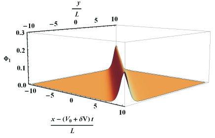
Figure 4: The ion-acoustic hump soliton structure (89) in a magnetized quantum plasma (moving with supersonic speed in the laboratory frame) is shown for normalized parameters: $\alpha=0.5,H^{2}=0.1,$ $\delta V=0.1$, $l_{x}=l_{y}=$ $\sqrt{2}/2$ and $g=0.22$ $(<1)$.

In order to investigate the valid range of the coefficients $A,$ $B$ and $C$ defined in Eqs.(85–87), respectively, for the existence of ion-acoustic soliton in a quantum magnetized plasma it is observed that $1<A<4/3$ for $1/3<\alpha<1$. Also, $H^{2}$ from Eq. (36) in principle can have large values due to which dispersive coefficients $B$ and $C$ do not remain positive definite in dense plasmas. The strong coupling effects associated with large values of $H^{2}$ can have its significant impact on the propagation of quantum ion-acoustic soliton, which could be addressed in a separate extended theory. Therefore, the existence or nonexistence of pure quantum ion-acoustic soliton in such a generalized study needs more precise statements. However, still some significant values of $H^{2}$ are physically acceptable in the present study. The two dimensional ion-acoustic potential hump (bright) soliton moving with supersonic speed in the laboratory frame is shown in Fig. 4 for plasma parameters for solid density i.e., $n_{0}=5\times 10^{30}\,\mathrm{m}^{-3},T=T_{F}=1.24\times 10^{6}\,\mathrm{K}$ and $B_{0}=10^{3}\,\mathrm{T}$ for which $\alpha=0.5,$ $H^{2}=0.1$.

IV Model for Magnetosonic Waves with Arbitrary Degeneracy of Electrons in Quantum Plasmas

In this section, we will investigate the magnetosonic waves in a magnetized quantum plasma with arbitrary degeneracy of electrons. The two fluid model is applied in which length scales remains less than the electron skin depth. The ions are assumed to be classical due to their large mass, while degenerate electrons contains Fermi pressure and quantum force due to wave like nature. This section is mainly a review from the material in (Haas and Mahmood 2018). The quantum fluid equations for magnetosonic waves in a dense plasma are described as follow.

The ion fluid continuity and momentum equations are given by

$$\frac{\partial n_{i}}{\partial t}+\mathbf{\nabla}\cdot\left(n_{i}\mathbf{v}_{i}\right)=0,$$ (93)

$$\frac{\partial\mathbf{v}_{i}}{\partial t}+\left(\mathbf{v}_{i}.\mathbf{\nabla}\right)\mathbf{v}_{i}=\frac{e}{m_{i}}\left(\mathbf{E}+\mathbf{v}_{i}\times\mathbf{B}\right),$$ (94)

where the ion fluid density and velocity are represented by $n_{i}$ and $\mathbf{v}_{i}$ respectively, while the ionic number density $\mathbf{E}$, $\mathbf{B}$ stands for the electromagnetic field, $m_{i}$ is the ions mass, and $-e$ is the electronic charge.

The continuity and momentum equations for electron quantum fluid is written as

$$\frac{\partial n_{e}}{\partial t}+\mathbf{\nabla}\cdot\left(n_{e}\mathbf{v}_{e}\right)=0,$$ (95)

$$\frac{\partial\mathbf{v}_{e}}{\partial t}+\left(\mathbf{v}_{e}.\mathbf{\nabla}\right)\mathbf{v}_{e}=-\frac{e}{m_{e}}\left(\mathbf{E}+\mathbf{v}_{e}\times\mathbf{B}\right)-\frac{1}{n_{e}m_{e}}\mathbf{\nabla}p+\left(\frac{\alpha}{3}\right)\frac{\hslash^{2}}{2m_{e}^{2}}\mathbf{\nabla}\left(\frac{1}{\sqrt{n_{e}}}\nabla^{2}\sqrt{n_{e}}\right),$$ (96)

where electron number density and fluid velocity are represented by $n_{e}$ and $\mathbf{v}_{e}$ , $m_{e}$ is the electron mass, $\hbar$ is the reduced Planck constant, $p$ is the electronic fluid pressure. The last term is the Bohm potential due to wave like nature of electrons and $\alpha$ is a numerical factor, which is set for comparison of results from fluid and kinetic theory in a 3D Fermi-Dirac distributed electrons plasma. The obtained expression of $\alpha$ in terms of fugacity $e^{\beta\mu_{(0)}}$ for low frequency waves is described in Eq.(31) and its numerical values in limiting cases are i.e., for classical plasma ($\alpha\approx 1$) and for fully degenerate case ($\alpha\approx 1/3$) .

In order to derive the equation of state for electron pressure, again we consider a local quasi-equilibrium Fermi-Dirac distribution function defined in Eq. (10). The relation between electron density $n_{e}$ and chemical potential $\mu$ is defined in Eq. (6), while the relation between equilibrium electron density and equilibrium chemical potential is defined in (8). Now using Eqs.(6) and (8), which gives a relation of electron density $n_{e}$ containing $n_{0}$, $\mu$ and $\mu_{(0)}$, which is used in Eq. (10) before inserting equation of state for electron pressure in Eq. (96).

The Faraday’s and Ampere’s laws are written as

$$\mathbf{\nabla}\times\mathbf{E}=-\frac{\partial\mathbf{B}}{\partial t},$$ (97)

$$\mathbf{\nabla}\times\mathbf{B}=\mu_{0}\mathbf{J+}\frac{1}{c^{2}}\frac{\partial\mathbf{E}}{\partial t},$$ (98)

where $\mu_{0}$ is the free space permeability and $c$ the speed of light. The current density is defined as

$$\mathbf{J}=e(n_{i}\mathbf{v}_{i}-n_{e}\mathbf{v}_{e}).$$ (99)

The charge neutrality condition $n_{i}\approx n_{e}$ is assumed and in equilibrium we have $n_{e,i}=n_{0}$, $\mathbf{v}_{e,i}=0$, $\mathbf{E}=0$ and $\mathbf{B}=B_{0}\hat{z}$, a uniform magnetic field. The magnetosonic waves are low frequency waves i.e., $\omega<<\Omega_{i}$, where $\Omega_{i}=eB_{0}/m_{i}$ is the ion gyro-frequency and also the displacement current in Eq. (98) will be ignored under the assumption that phase speed of the wave is much less than the speed of light.

IV.1 Linear Analysis

In order to find the dispersion relation of the magnetosonic waves in a magnetized quantum plasma with arbitrary degeneracy of electron, we have to linearized the set dynamic Eqs.(93)-(99). The external magnetic field is assumed to be directed along $z$-axis i.e., $\mathbf{B}_{0}=B_{0}\hat{z}$ and wave propagation is taken along x-axis i.e., $\mathbf{\nabla=(\partial}_{x},0,0)$. The electric field lies in the XY-plane i.e., $\mathbf{E}=E_{x}\hat{x}+E_{y}\hat{y}$ and magnetic field is $\mathbf{B}=(B_{0}+B_{z})\hat{z}$. Now assuming the sinusoidal perturbations of the form $\exp\left(ikx-i\omega t\right)$, the obtained dispersion relation of magnetosonic waves in dense magnetized plasma is given by

$$\omega^{2}=\left(c_{s}^{2}+\frac{\alpha}{12}\frac{\hslash^{2}}{m_{i}m_{e}}k^{2}\right)k^{2}+\frac{k^{2}v_{A}^{2}}{1+k^{2}\lambda_{e}^{2}},$$ (100)

where $c_{s}$ is the ion-acoustic speed defined in Eq. (23) and $v_{A}=B_{0}/\sqrt{\mu_{0}m_{i}n_{0}}$ is the Alfvén speed. The electron skin depth $\lambda_{e}=\sqrt{c/\omega_{pe}}$ is defined, where $\omega_{pe}=\sqrt{n_{0}e^{2}/(m_{e}\varepsilon_{0})}$ is the electrons plasma frequency with $\varepsilon_{0}$ being the free space permittivity.

In case of short wavelength i.e., $k^{2}\lambda_{e}^{2}>>1$, the magnetosonic dispersion relation (100) gives,

$$\omega^{2}=\left(c_{s}^{2}+\frac{\alpha}{12}\frac{\hslash^{2}}{m_{i}m_{e}}k^{2}\right)k^{2}+\Omega_{i}\Omega_{e},$$ (101)

which is the lower hybrid frequency mode in a magnetized plasma modified in the presence quantum effects. Here $\Omega_{j}=eB_{0}/m_{j}$ (here $j=i,e$) is the gyrofrequency of the plasma species.

It can be seen from dispersion relation (100) that wave dispersion effects appears due to finite electron skin depth $\lambda_{e}$ and inclusion of Bohm potential effects in the model. The phase velocity of the magnetosonic waves in the absence of Bohm term and in the long wavelength ( $k^{2}\lambda_{e}^{2}<<1$) is given by

$$\frac{\omega}{k}=\sqrt{c_{s}^{2}+v_{A}^{2}},$$ (102)

The limiting case analysis of non-degenerate and fully degenerate magnetized plasmas of obtained dispersion relation of magnetosonic waves in a quantum plasma with arbitrary degeneracy of electrons is done below:

In case of dilute plasma case with a small fugacity $e^{\beta\mu_{(0)}}\ll 1$ and ignoring the Bohm potential, then dispersion relation (100) gives,

$$\omega^{2}=c_{s}^{2}k^{2}+\frac{k^{2}v_{A}^{2}}{1+k^{2}\lambda_{e}^{2}},$$ (103)

which is the same as Eq. (16) in Ref. (Ur-Rehman et al. 2017), while ion-acoustic speed is $c_{s}=\sqrt{\kappa_{B}T/m_{i}}$ defined for a classical plasma.

However, for fully degenerate plasma case i.e., fugacity $e^{\beta\mu_{(0)}}\ll 1$, the dispersion relation (100) for magnetosonic waves is written as

$$\omega^{2}=\left(c_{s}^{2}+\frac{\hslash^{2}}{36m_{i}m_{e}}k^{2}\right)k^{2}+\frac{k^{2}v_{A}^{2}}{1+k^{2}\lambda_{e}^{2}},$$ (104)

where $c_{s}=\sqrt{2\varepsilon_{F}/(3m_{i})}$ is the ion-acoustic speed in a quantum plasma, while $\varepsilon_{F}=\kappa_{B}T_{F}=[\hbar^{2}/(2m_{e})]\,(3\pi^{2}n_{0})^{2/3}$ is the Fermi energy of electrons and in fully degenerate plasmas $\mu_{(0)}=\varepsilon_{F}$.

IV.2 Derivation of a KdV equation for magnetosonic solitons in dense plasmas with arbitrary degeneracy of electrons

In order to derive the KdV equation for magnetosonic solitons in dense plasma with arbitrary degeneracy of electrons, the set of dynamic equations (93)-(99) can be written in normalized form as follows:

The ion continuity equation is written as

$$\frac{\partial\tilde{n}_{i}}{\partial\tilde{t}}+\frac{\partial}{\partial\tilde{x}}\left(\tilde{n}_{i}\tilde{v}_{ix}\right)=0.$$ (105)

The ion momentum equation along $x$ and $y$ axis are described by

$$\frac{\partial\tilde{v}_{ix}}{\partial\tilde{t}}+\tilde{v}_{ix}\frac{\partial}{\partial\tilde{x}}\tilde{v}_{ix}=\tilde{E}_{x}+\Omega\text{ }\tilde{v}_{iy}\tilde{B},$$ (106)

$$\frac{\partial\tilde{v}_{iy}}{\partial\tilde{t}}+\tilde{v}_{ix}\frac{\partial}{\partial\tilde{x}}\tilde{v}_{iy}=\tilde{E}_{y}-\Omega\text{ }\tilde{v}_{ix}\tilde{B}.$$ (107)

The continuity equation of electron is written as

$$\frac{\partial\tilde{n}_{e}}{\partial\tilde{t}}+\frac{\partial}{\partial\tilde{x}}\left(\tilde{n}_{e}\tilde{v}_{ex}\right)=0,$$ (108)

The $x$ and $y$ components of the electron fluid momentum equation are given by

$$\left.\frac{\partial\tilde{v}_{ex}}{\partial\tilde{t}}+\tilde{v}_{ex}\frac{\partial}{\partial\tilde{x}}\tilde{v}_{ex}=-\delta\text{ }\tilde{E}_{x}-\delta\text{ }\Omega\text{ }\tilde{v}_{ey}\tilde{B}\right.-\delta\text{ }\frac{\mathrm{Li}_{1/2}(-e^{\beta\mu_{(0)}})}{\mathrm{Li}_{1/2}(-e^{\beta\mu})}\frac{\partial}{\partial\tilde{x}}\tilde{n}_{e}$$

$$\left.+\frac{1}{2}\delta\text{ }H^{2}\text{ }\frac{\partial}{\partial\tilde{x}}\left(\frac{1}{\sqrt{\tilde{n}_{e}}}\frac{\partial^{2}}{\partial\tilde{x}^{2}}\sqrt{\tilde{n}_{e}}\right),\right.$$ (109)

$$\frac{\partial\tilde{v}_{ey}}{\partial\tilde{t}}+\tilde{v}_{ex}\frac{\partial}{\partial\tilde{x}}\tilde{v}_{ey}=-\delta\text{ }\tilde{E}_{y}+\delta\text{ }\Omega\text{ }\tilde{v}_{ex}\tilde{B}.$$ (110)

The $z$ component of the Faraday’s law yields

$$\frac{\partial\tilde{E}_{y}}{\partial\tilde{x}}=-\Omega\text{ }\frac{\partial\tilde{B}}{\partial\tilde{t}}.$$ (111)

The $x$ and $y$ components of Ampere’s law are written as

$$0=\tilde{n}_{i}\tilde{v}_{ix}-\tilde{n}_{e}\tilde{v}_{ex},$$ (112)

$$\Omega\text{ }\frac{\partial\tilde{B}}{\partial\tilde{x}}=\frac{c_{s}^{2}}{c^{2}}\left(\tilde{n}_{e}\tilde{v}_{ey}-\tilde{n}_{i}\tilde{v}_{iy}\right).$$ (113)

The normalization of electron and ion fluid density and fluid velocities are defined as $\tilde{n}_{e,i}=n_{e,i}/n_{0}$ and $\mathbf{\tilde{v}}_{e,i}=\mathbf{v}_{e,i}/c_{s}$, respectively. Also, the normalization of space, time, electric and magnetic fields i.e., $\tilde{x}=\omega_{pi}\,x\mathbf{/}c_{s}$,$\ \tilde{t}=\omega_{pi}t$,$\ \tilde{\mathbf{E}}\mathbf{=}e\mathbf{E}\mathbf{/}\left(m_{i}c_{s}\omega_{pi}\right)$ and $\tilde{\mathbf{B}}=B\hat{z}\mathbf{/}B_{0}$ are defined. The dimensionless quantum diffraction parameter $H$ is defined in Eq. (36) and $\delta=m_{i}/m_{e}$ is the ion-electron mass ratio defined in Eq. (109). The ratio of ion-cyclotron to ion plasma frequencies is defined as $\Omega=\Omega_{i}/\omega_{pi}$, where ion plasma frequency is $\omega_{pi}=\sqrt{e^{2}n_{0}/(m_{i}\varepsilon_{0})}$. The normalized electron density ($\tilde{n}_{e}$) with chemical potential ($\mu$) are related through relation described in Eq. (37). In further calculations, the tilde sign on normalized variables will not be used for simplicity.

The well known reductive perturbation method is employed (Hussain and Mahmood 2017) to find the KdV equation and stretching spatial and temporal independent variables is defined as follows,

$$\xi=\epsilon^{1/2}(x-v_{0}t)\text{, \ \ \ \ \ \ \ \ \ \ \ \ }\tau=\epsilon^{3/2}t.$$

Here $\epsilon$ is a small expansion parameter which characterizes the strength of nonlinearity and $v_{0}$ is the normalized phase velocity of the wave to be determined later on.

The expansion of dynamic variables expanded in terms of the smallness parameter $\epsilon$ is defined below (where $j=e,i$),

$$n_{j} =1+\epsilon n_{j1}+\epsilon^{2}n_{j2}+...$$

$$v_{jx} =\epsilon v_{jx1}+\epsilon^{2}v_{jx2}+...$$

$$v_{jy} =\epsilon^{3/2}v_{jy1}+\epsilon^{5/2}v_{jy2}+...$$

$$E_{x} =\epsilon^{3/2}E_{x1}+\epsilon^{5/2}E_{x2}+...$$

$$E_{y} =\epsilon E_{y1}+\epsilon^{2}E_{y2}+...$$

$$B =1+\epsilon B_{z1}+\epsilon^{2}B_{z2}+....$$

$$\mu =\mu_{(0)}+\epsilon\mu_{1}+\epsilon^{2}\mu_{2}+...$$ (114)

Now applying the perturbation scheme in Eqs. (106) to (113) and collecting the lowest order terms, which gives normalized phase velocity of the wave as follows:

$$v_{0}=\pm\sqrt{1+\frac{v_{A}^{2}}{c_{s}^{2}}},$$ (115)

which is the same phase velocity of the wave as already derived in Eq. (102) for a dispersionless wave. The positive sign of $v_{0}$ will be retained in further calculations without any loss of generality.

Now collecting the next higher order ($\varepsilon$) terms from the set of dynamic equations and on solving them we obtain,

$$\frac{f_{2}}{v_{0}}+f_{3}+\frac{f_{5}}{\delta}-\frac{\Omega c^{2}}{c_{s}^{2}}f_{9}-\frac{\Omega c^{2}}{v_{0}c_{s}^{2}}f_{7}+\frac{1}{\delta}\left(\frac{\Omega c^{2}}{v_{0}c_{s}^{2}}\right)\frac{\partial f_{6}}{\partial\xi}=0.$$ (116)

Equation (115) has been used in the derivation of Eq. (116) and the expression of $f_{1}$ to $f_{9}$ are described in the Appendix.

In order to express the first order perturbed quantities $v_{ix1}$, $n_{i1}$, $n_{e1}$, $B_{z1}$, $E_{x1}$, $E_{y1}$, $v_{iy1}$ and $v_{ey1}$ in terms of one variable $v_{ex1}$, we have

$$E_{y1}=\Omega v_{ex1},$$ (117)

$$v_{ix1}=v_{ex1},$$ (118)

$$n_{i1}=n_{e1}=\frac{v_{ex1}}{v_{0}},$$ (119)

$$B_{z1}=\frac{v_{ex1}}{v_{0}},$$ (120)

$$E_{x1}=-\frac{1}{v_{0}\delta}\left(v_{0}^{2}\,\delta+1\right)\frac{\partial v_{ex1}}{\partial\xi}\approx-v_{0}\frac{\partial v_{ex1}}{\partial\xi},$$ (121)

$$v_{iy1}=\frac{1}{\Omega v_{0}\delta}\frac{\partial v_{ex1}}{\partial\xi},$$ (122)

$$v_{ey1}=\frac{1}{\Omega v_{0}}\left(v_{0}^{2}+1\right)\frac{\partial v_{ex1}}{\partial\xi},$$ (123)

where the relation $v_{ey1}=-\delta\,v_{iy1}$ between electron and ion momentum along $y$ direction has also been used  to derive the above relations. Also, the approximations $\delta\gg 1,v_{0}>1$ has been used to obtain relation (121).

Using relations (117)-(123) in Eq. (116) and after some simplification, the KdV equation is obtained for magnetosonic waves in a quantum plasma in terms $v_{ex1}$ is given by

$$\frac{\partial v_{ex1}}{\partial\tau}+aa\text{ }v_{ex1}\frac{\partial v_{ex1}}{\partial\xi}+bb\text{ }\frac{\partial^{3}v_{ex1}}{\partial\xi^{3}}=0,$$ (124)

where the nonlinearity and dispersion coefficients $aa$ and $bb$ are defined as

$$aa=\frac{1}{2}\left[3-\frac{1}{v_{0}^{2}}\left(\frac{1}{\delta}+\alpha\right)\right]\approx\frac{1}{2}\left(3-\frac{\alpha}{v_{0}^{2}}\right)>0,$$ (125)

$$bb=\frac{1}{2v_{0}}\left(\frac{\Omega^{2}c^{4}}{\delta\,\,c_{s}^{4}}-\frac{H^{2}}{4}\right).$$ (126)

The nonlinearity coefficient $aa>0$ is a definite positive because $\alpha\leq 1$, $v_{0}\geq 1$. The KdV equation (124) gives a shock solution instead of soliton if dispersion coefficient $bb$ vanishes, which could happen at $H=2\Omega c^{2}/\left(\sqrt{\delta}c_{s}^{2}\right)$. After some simplification, the shock condition can be written as follows

$$bb=0\Rightarrow m_{e}m_{i}\lambda_{e}^{2}v_{A}^{2}=\frac{\alpha\hbar^{2}}{12},$$ (127)

It should be noted here that when the dispersion coefficient $bb$ vanishes, the leading dispersion contribution appears at a higher order, including a fifth-order spatial derivative term, yielding the Kawahara equation (Kawahara 1972), a possible application of the obtained shock condition.

The limiting cases of KdV equation (124) for magnetosonic waves in a quantum plasma as discussed here: in dilute plasma case $e^{\beta\mu_{(0)}}\ll 1$, we have

$$\frac{\partial v_{ex1}}{\partial\tau}+\frac{(2u_{m}^{2}+v_{A}^{2})}{2u_{m}^{2}}\text{ }v_{ex1}\frac{\partial v_{ex1}}{\partial\xi}+\frac{\omega_{pi}^{2}}{2u_{m}c_{s}^{3}}\left(\lambda_{e}^{2}v_{A}^{2}-\frac{\hbar^{2}}{12m_{e}m_{i}}\right)\text{ }\frac{\partial^{3}v_{ex1}}{\partial\xi^{3}}=0,$$ (128)

where magnetosonic and ion-acoustic waves speeds are defined as $u_{m}=\sqrt{v_{A}^{2}+c_{s}^{2}}$ and $c_{s}=\sqrt{\kappa_{B}T/m_{i}}$ respectively. Equation (128) is the same as Eq. (30) of Ref. (Ohsawa and Sakai 1987), when  (128) is re-written in dimensional form and replacing $v_{ex1}$ in terms of the first order perturbed electron density $n_{e1}$ using relation (119), and also neglecting quantum diffraction effects in the model.

The obtained shock condition ($bb=0$) in the dilute plasma case is

$$\frac{\Omega_{e}}{\omega_{pe}}=\frac{\hbar\omega_{pe}}{2\sqrt{3}\,m_{e}c^{2}}\,.$$ (129)

or

$$\frac{n_{0}}{B_{0}}=1.49\times 10^{29}\,\mathrm{m}^{-3}\,{\mathrm{T}}^{-1}\,,$$ (130)

in terms of SI units. The shock condition in a dilute plasma depends only on plasma density and magnetic field intensity as long as $T\ll T_{F}$ holds. The equality is quite applicable to laboratory or astrophysical plasma situations.

However, in a fully degenerate plasma case ($e^{\beta\mu_{(0)}}\ll 1$), the KdV equation (124) gives

$$\frac{\partial v_{ex1}}{\partial\tau}+\frac{(8u_{m}^{2}+v_{A}^{2})}{6u_{m}^{2}}\text{ }v_{ex1}\frac{\partial v_{ex1}}{\partial\xi}+\frac{\omega_{pi}^{2}}{2u_{m}c_{s}^{3}}\left(\lambda_{e}^{2}v_{A}^{2}-\frac{\hbar^{2}}{36m_{e}m_{i}}\right)\text{ }\frac{\partial^{3}v_{ex1}}{\partial\xi^{3}}=0,$$ (131)

where $c_{s}=\sqrt{2\varepsilon_{F}/(3m_{i})}$ is the ion-acoustic speed in a quantum plasma and $H=\hslash\omega_{pe}/(2\kappa_{B}T_{F})$. The obtained shock condition in a fully degenerate plasma case is given by

$$\frac{\Omega_{e}}{\omega_{pe}}=\frac{\hbar\omega_{pe}}{6\,m_{e}c^{2}}\,,$$ (132)

or

$$\frac{n_{0}}{B_{0}}=2.58\times 10^{29}\,\mathrm{m}^{-3}\,{\mathrm{T}}^{-1}\,.$$ (133)

The traveling wave solution of KdV Eq. (124) for one soliton is given by

$$v_{ex1}=\Psi_{0}\,\mathrm{sech}^{2}\left(\frac{\eta}{\Delta}\right).$$ (134)

where $\eta=\xi-u_{0}\tau$, is the transformed coordinate in the co-moving frame and $u_{0}$ is the soliton velocity. A single pulse soliton solution is obtained by applying decaying boundary conditions i.e., $v_{ex1}$, $\partial v_{ex1}/\partial\eta$ and $\partial^{2}v_{ex1}/\partial\eta^{2}$ $\rightarrow 0$ as $\eta\rightarrow\pm\infty$. Here $\Psi_{0}$ is the height and $\Delta$ is the width of magnetosonic soliton, which are defined as

$$\Psi_{0}=\frac{3u_{0}}{aa},\text{ \ \ \ \ \ \ \ }\Delta=\sqrt{\frac{4\text{ }bb}{u_{0}}}.$$ (135)

It is can be seen from dispersive coefficient $bb$, which contains quantum diffraction effects defined in Eq.(125), both hump (bright) or dip (dark) magnetosonic soliton are possible depending on the sign of $bb$. The height  of the soliton contains nonlinearity coefficient $aa$ which depends on quantum degeneracy effects only and remains positive. On condition $H^{2}/4<(\Omega^{2}c^{4}/\delta c_{s}^{4})$, the dispersive coefficient $bb>0$ holds for which soliton velocity $u_{0}>0$ remains valid for real positive values of the soliton width. Therefore, a bright magnetosonic soliton moving with supersonic speed is formed. However, if the dispersive coefficient has negative values i.e., $bb<0$, which could happens at $H^{2}/4>(\Omega^{2}c^{4}/\delta c_{s}^{4})$ then soliton velocity $u_{0}<0$ should hold for the validity of the soliton solution (134) (Belashov and Vladimirov 2005; Haas and Mahmood, 2015;2016;2018). Therefore at these conditions there is possibility of dark soliton moving with subsonic speed. The variation of dispersive coefficient $bb$ with thermal temperature is plotted at different magnetic field intensities in Fig.5 for arbitrary degenerate electrons plasmas. It is evident from the numerical plot that the dispersive coefficient $bb<0$ holds for electron temperatures of the order of magnitude $T>10^{6}$ K and dark magnetosonic solitons moving with subsonic speed are formed. The range of electron temperature for the formation of dark soliton structure is reduced with increase in the magnetic field intensity as shown in the figure.

Figure 5: Dispersive coefficient $bb$  of KdV equation for magnetosonic wave is shown as a function of electron temperature from Eq. (126) for $B_{0}=3$ $\mathrm{T}$ (lower, solid curve) and $B_{0}=6$ $\mathrm{T}$ (upper, dotted curve) at $z=1$.

V Numerical Estimates and Applications

In this section, the numerical estimates of the physical dense parameters will be found out for the propagation of linear and nonlinear waves in arbitrary degenerate electron plasma. The material reviews the presentation in (Haas and Mahmood 2018). According to our general presented theory of arbitrary degeneracy of electrons, which lies in the intermediate range where the thermal and Fermi temperature are almost equal i.e.,

$$T=T_{F}\,,$$ (136)

where electrons Fermi temperature $T_{F}=\varepsilon_{F}/\kappa_{B}$ is defined in terms of Fermi energy.

In order to find numerical estimates of the fugacity $z=$ $e^{\beta\mu_{(0)}}$and coefficient $\alpha$ for the intermediate range, the relation (8) can be re-written (Eliasson and Shukla 2008) as follows,

$$\mathrm{Li}_{3/2}(-z)=-\frac{4}{3\sqrt{\pi}}\,(\beta\varepsilon_{F})^{3/2}\,,$$ (137)

Accordingly intermediate dense plasmas in which electron thermal and Fermi temperature are equal, therefore $\beta\varepsilon_{F}=1$ for which equilibrium fugacity comes out to be $z=0.98$ from Eq.(137) and $\alpha=0.80$ from Eq.(31). It is also evident from Fig.2 that $\alpha=0.80$ lies in the intermediate dilute-degenerate plasma situation.

The two phenomenon such as quantum degeneracy through electron Fermi pressure and quantum diffraction effects due to wave like nature of electrons are included in the model. The quantum diffraction effects gives extra dispersion of linear wave in dense plasmas and modified the width of the soliton structure. The quantum diffraction parameter $H$ plays an important role in the formation of bright or dark soliton in magnetized dense plasmas. Theoretically speaking the dark soliton are formed for the large values of quantum diffraction parameter $H$ which in reality cannot be increased with limits under the present ideal Fermi-gas model. In fact for large values of $H$ one would enter to strongly plasma regime which is not applicable to the present model. Therefore in order to find the validity range of quantum diffraction parameter $H$, the coupling parameter $g$ is analyzed such that $g=l/r_{s}$, and

$$l=-\frac{e^{2}}{12\pi\varepsilon_{0}\kappa_{B}T}\,\frac{n_{0}\Lambda_{T}^{3}}{\mathrm{Li}_{5/2}(-z)}\text{.}$$ (138)

Here $l$ is a generalized Landau length (Kremp et al. 2005; Ichimaru 2004; Lifshitz 1981) involving the thermal de Broglie wavelength $\Lambda_{T}=[2\pi\hbar^{2}/(m_{e}\kappa_{B}T)]^{1/2}$, and $r_{s}=(4\pi n_{0}/3)^{-1/3}$ is the Wigner-Seitz radius.

In the dilute plasma case, one has $e^{2}/(4\pi\varepsilon_{0}\,l)=(3/2)\kappa_{B}T$, so that $l$ would be the classical distance of closest approach in a binary collision, for average kinetic energy. The degeneracy effects have been incorporated in the mean kinetic energy as described in (138). It could be noticed that indiscriminate increase in the quantum value of $H$ enhances the non-ideality effects such as bound states and dynamical screening (Kremp et al. 2005). Therefore it can be concluded that the dark soliton and shock wave solutions of KdV and ZK equations, which theoretically needs large values of quantum diffraction parameter i.e., $H>2$ lies in the outside range of ideal (or less collisional) dense plasma situation i.e., $g<1$. However, there is still possibility that wave nature of electrons associated with quantum diffraction parameter provides important corrections for the least reasonable values of $H$.

Now in order to find the estimates of the range of minimum to maximum wavelengths of the wave as a function of electron Fermi energy in the intermediate-dilute degenerate plasma, for the consistency of our present investigation, we have from Eq. (27) of (Haas and Mahmood 2015) i.e.,

$$k_{\mathrm{min}}\equiv\frac{2\sqrt{3}m_{e}c_{s}}{\hbar}\ll k\ll\frac{\omega_{pi}}{c_{s}}\equiv k_{\mathrm{max}}\,.$$ (139)

The above equation has been obtained under long wavelength assumption from fluid model and static response of electrons. In case of hydrogen plasma and $T=T_{F}$, we have $k_{\mathrm{max}}>k_{\mathrm{min}}$ for $n_{0}<9.81\times 10^{35}\,\mathrm{m}^{-3}$ (solid density) from Eq. (139). The dense plasma density lies in the nonrelativistic regime, according to our present study. The first in equality in Eq. (139) can be ignored if the quantum degeneracy effects are more dominant then the quantum diffraction effects. The suitable range of wavelength $\lambda_{\mathrm{min}}=2\pi/k_{\mathrm{max}}\ll\lambda\ll\lambda_{\mathrm{max}}=2\pi/k_{\mathrm{min}}$ as a function of electron energy for intermediate dilute degenerate hydrogen plasma as a function of electron Fermi energy is plotted in Fig.6, which lies in the nanometric scale from extreme ultraviolet to soft X-rays. However, in case of high densities exist in compact astrophysical objects like white dwarfs and neutron stars, electron Fermi momentum becomes comparable to $m_{e}c$ and dense plasma needs relativistic treatment which beyond the scope of our present studies.

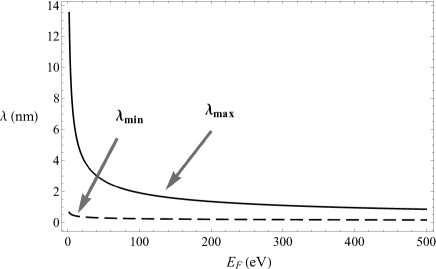
Figure 6: Upper, continuous curve: maximum wavelength $\lambda_{\mathrm{max}}$; lower, dashed curve: minimal wavelength $\lambda_{\mathrm{min}}$, consistent with Eq. (139) are plotted as a function of the electronic Fermi energy $\varepsilon_{F}$ in $\mathrm{eV}$, for hydrogen plasma in the intermediate dilute-degenerate regime where $T=T_{F}$ holds.

In order to justify the cold and nondegenerate ideal ionic fluid and avoiding the strong ion coupling effects, the necessary condition for ionic coupling parameter (Kremp et al. 2005) is defined as

$$g_{i}=\frac{e^{2}}{4\pi\varepsilon_{0}r_{s}}\,\left(\frac{3\kappa_{B}T_{i}}{2}\right)^{-1}\ll 1\,$$ (140)

where $T_{i}$ is the the ion thermal temperature and $T_{i}<T_{F}$ should hold. It is believed that for $g_{i}\approx 172$ in one-component plasma the ionic liquid or crystallization start to happen (Murillo 2004). The allowable region between the two straight lines $T_{i}=T_{F}$ and $g_{i}=1$ for cold and weakly coupled ions is shown in Fig.7. The minimum number density of cold and weakly coupled ions comes out to be $n_{0}=3.63\times 10^{28}\,\mathrm{m}^{-3}$ which lies in the range of typical solid density plasmas.

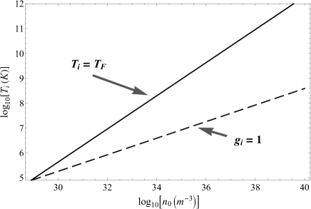
Figure 7: The cold and weakly coupled ions region below the upper, continuous straight line (where the ionic temperature $T_{i}$ equals the electronic Fermi temperature $T_{F}$) and above the lower, dashed straight line (where the ionic coupling parameter $g_{i}=1$) is shown using Eq. (140).

VI Conclusion

The main findings our present investigation to study the linear and nonlinear ion-acoustic waves and magnetosonic waves in a quantum plasma with arbitrary degeneracy of electrons. The equation of state for arbitrary degeneracy of electrons is found out in the form of polylogarithms obtained by using Fermi-Dirac integral, which is a function of both chemical potential and temperature. It’s limiting cases for dilute and dense plasma regions are also discussed. A dimensionless parameter ($\alpha$), which involves dimensionality and temperature, is defined in front of quantum force in electron momentum quantum fluid equation to fit the results obtained from quantum kinetic theory in the long wavelength limit. A mathematical relation of $\alpha$ in the form of polylogarithms function of equilibrium chemical potential and temperature is obtained its numerical values are found out in the limiting cases for dilute and dense plasmas. The KdV equation for ion-acoustic waves in unmagnetized quantum plasma with arbitrary degeneracy of electrons with its soliton solution is obtained. The bright IAW soliton in unmagnetized quantum plasma is formed for the quantum diffraction values $H<2$ (moving with supersonic speed), while dark soliton structure is formed for $H>2$ (moving with subsonic speed). The ion-acoustic wave dispersion effects in unmagnetized quantum plasma appears only through quantum diffraction effects from Bohm potential.

The ZK equation for two dimensional propagation of ion-acoustic soliton is also obtained in a magnetized quantum plasma with arbitrary degeneracy of electrons. It is found that wave dispersion effects appear through quantum diffraction parameter ($H$) and ion Larmour radius effect in the perpendicular direction of the magnetic field. The conditions for existence of bright or dark ZK ion-acoustic solitons in a magnetized quantum plasma with quantum diffraction parameter and magnetic field intensity are discussed in detail. Similarly, the KdV equation for weakly nonlinear magnetosonic waves in a quantum plasma with finite temperature effects of electrons is also studied. It is found that both bright or (dark) magnetosonic soliton structures are possible moving with supersonic and (subsonic) speeds in a magnetized quantum plasma depending on the plasma density, electron temperature and magnetic field intensity. Other than solitons, the shock wave solution with its conditions for formation depending on the values of quantum diffraction parameter and magnetic field intensity are also discussed. Also, a general coupling parameter in the form of polylogarithms is proposed and conditions for ideal (or collisionless) dilute or dense plasmas are worked out. The mathematical expressions of minimal criteria for the electron temperature and maximal quantum diffraction parameter on the formation of dark solitons for the ideality and weak coupling system having arbitrary degeneracy of electrons are also discussed and their physical conditions for real systems are also pointed out. The physical parameters of hydrogen plasmas in the intermediate dilute-degenerate limits where $T=T_{F}$ holds for fully ionized electron case with arbitrary temperature of degenerate electrons are also presented. It is found that for hydrogen plasmas (solid-density) with arbitrary degeneracy of electrons, the wavelength ($\sim$ nanometer scale) of plasma waves lies in the range from extreme ultraviolet to soft x rays. Therefore, we are hopeful that the physical parameters developed form our present theory will be useful for experimental and observational verifications of linear and nonlinear ion-acoustic and magnetosonic waves in laboratory and in nature with large range of electron degeneracy regime.

Acknowledgments: F. H.  acknowledges the support by Conselho Nacional de Desenvolvimento Científico e Tecnológico (CNPq).

This version is faithful (unconstrained by unfair refereeing).

Appendix: Functions defined after collecting first and second order terms from perturbation theory

The functions $f_{1}$ to $f_{9}$ defined in the equation (116) are given as follows:

$$f_{1}=\frac{\partial n_{i1}}{\partial\tau}+\frac{\partial}{\partial\xi}\left(n_{i1}v_{ix1}\right)\,,\text{ \ \ \ \ \ \ \ \ \ \ \ \ \ \ \ \ \ \ }f_{2}=\frac{\partial n_{e1}}{\partial\tau}+\frac{\partial}{\partial\xi}\left(n_{e1}v_{ex1}\right)\,,$$ (a1)

$$f_{3}=\frac{\partial v_{ix1}}{\partial\tau}+v_{ix1}\frac{\partial}{\partial\xi}v_{ix1}-\Omega\text{ }v_{iy1}B_{z1}\,,\text{ \ \ \ \ \ \ \ \ \ \ \ \ }f_{4}=-v_{0}\frac{\partial v_{ix1}}{\partial\xi}+\Omega\text{ }v_{ix1}B_{z1}\,,$$ (a3)

$$f_{5}=\frac{\partial v_{ex1}}{\partial\tau}+v_{ex1}\frac{\partial}{\partial\xi}v_{ex1}+\delta\,\Omega\text{ }v_{ey1}B_{z1}-\delta\,\alpha\text{ }n_{e1}\frac{\partial n_{e1}}{\partial\xi}-\delta\,\frac{H^{2}}{4}\text{ }\frac{\partial^{3}n_{e1}}{\partial\xi^{3}}\,,$$ (a5)

$$f_{6}=-v_{0}\frac{\partial v_{ey1}}{\partial\xi}+\Omega\text{ }v_{ex1}B_{z1}\,,\text{ \ \ \ \ \ \ \ }f_{7}=-\Omega\frac{\partial B_{z1}}{\partial\tau}\,,$$ (a6)

$$f_{8}=\left(n_{e1}-n_{i1}\right)v_{ex1}\,,\text{ \ \ \ \ \ \ \ \ \ \ \ \ \ \ \ \ \ \ \ \ \ \ \ \ \ \ }f_{9}=\frac{c_{s}^{2}}{c^{2}}\left(n_{e1}v_{ey1}-n_{i1}v_{iy1}\right)\,.$$ (a8)

References

- (1) L. Lewin, Polylogarithms and Associated Functions (North-Holland, New York, 1981).
- (2) R. K. Pathria, P. D. Beale, Statistical Mechanics - 3rd ed. (Elsevier, New York, 2011).
- (3) G. Manfredi, J. Hurst, Solid state plasmas. Plasma Phys. Control. Fusion 57, 054004 (2015).
- (4) J. E. Cross, B. Reville, G. Gregori, Scaling of magneto-quantum-radiative hydrodynamics equations: from laser-produced plasmas to astrophysics. Astrophys. J. 795, 59 (2014).
- (5) F. Haas, Quantum Plasmas: an Hydrodynamic Approach (Springer, New York, 2011).
- (6) N. Maafa, Dispersion relation in a plasma with arbitrary degeneracy, Physica Scripta 48, 351 (1993).
- (7) A. Mushtaq, D. B. Melrose, Quantum effects on the dispersion of ion-acoustic waves. Phys. Plasmas 16, 102110 (2009).
- (8) D. B. Melrose, A. Mushtaq, Dispersion in a thermal plasma including arbitrary degeneracy and quantum recoil. Phys, Rev. E 82, 056402 (2010).
- (9) B. Eliasson, P. K. Shukla, Nonlinear quantum fluid equations for a finite temperature Fermi plasma. Physica Scripta 78, 025503 (2008).
- (10) A. E. Dubinov, A. A. Dubinova, M. A. Sazokin, Nonlinear theory of the isothermal ion–acoustic waves in the warm degenerate plasma. J. Commun. Tech. Elec. 55, 907 (2010).
- (11) A. E. Dubinov, I. N. Kitaev, Non-linear Langmuir waves in a warm quantum plasma. Phys. Plasmas 21, 102105 (2014).
- (12) B. Eliasson, M. Akbari-Mghanjoughi, Finite temperature static charge screening in quantum plasmas, Phys. Lett. A 380, 2518 (2016).
- (13) F. Haas, S. Mahmood, Linear and nonlinear ion-acoustic waves in non-relativistic quantum plasmas with arbitrary degeneracy. Phys. Rev. E 92, 053112 (2015).
- (14) H. L. Rubin, T. R. Govindan, J. P. Kreskovski, M. A. Stroscio, Transport via the Liouville equation and moments of quantum distribution functions. Solid St. Electron 36, 1697 (1993).
- (15) J. R. Barker, D. K. Ferry, On the validity of quantum hydrodynamics for describing antidot array devices. Semicond. Sci. Technol. 13, A135 (1998).
- (16) C. L. Gardner, The quantum hydrodynamic model for semiconductor devices. SIAM J. Appl. Math. 54, 409 (1994).
- (17) A. I. Akhiezer, I. A. Akhiezer, R. V. Polovin, A. G. Sitenko and K. N. Stepanov, Plasma Electrodynamics, Vol. I & II (Pergamon, Oxford, 1975).
- (18) P. K. Shukla, B. Eliasson, Colloquium: nonlinear collective interactions in quantum plasmas with degenerate electron fluids. Rev. Mod. Phys. 83, 885 (2011).
- (19) A. P. Misra, P. K. Shukla, Stability and evolution of wave packets in strongly coupled degenerate plasmas. Phys. Rev. E 85, 026409 (2012).
- (20) B. Eliasson, P.K. Shukla, Dispersion properties of electrostatic oscillations in quantum plasmas. J. Plasma Phys. 76, 7 (2010).
- (21) D. Michta, F. Graziani, M. Bonitz, Quantum hydrodynamics for plasmas – a Thomas-Fermi theory perspective. Contrib. Plasma Phys. 55, 437 (2015).
- (22) M. Akbari-Moghanjoughi, Hydrodynamic limit of Wigner-Poisson kinetic theory: revisited. Phys. Plasmas 22, 022103 (2015).
- (23) D. Bohm, D. Pines, A collective description of electron interactions: III. Coulomb interactions in a degenerate electron gas. Phys. Rev. 92, 609 (1953).
- (24) F. Haas, L. G. Garcia, J. Goedert, G. Manfredi, Quantum ion-acoustic waves. Phys. Plasmas 10, 3858 (2003).
- (25) S. Mahmood, F. Haas, Ion-acoustic cnoidal waves in a quantum plasma. Phys. Plasmas 21, 102308 (2014).
- (26) R. C. Davidson, Methods in Nonlinear Plasma Theory (Academic Press New York, 1972).
- (27) T. Kawahara, Oscillatory solitary waves in dispersive media. Phys. Soc. Jpn. 33, 260 (1972).
- (28) V. Yu. Belashov, S. V. Vladimirov, Solitary Waves in Dispersive Complex Media (Springer, Berlin-Heidelberg, 2005).
- (29) F. Haas, S. Mahmood, Nonlinear ion-acoustic solitons in a magnetized quantum plasma with arbitrary degeneracy of electrons. Phys. Rev. E 94, 033212 (2016).
- (30) T. E. Stringer, Low-frequency waves in an unbounded plasma. J. Nucl. Energy Part C 5, 89 (1963).
- (31) E. Witt, W. Lotko, Ion-acoustic solitary waves in a magnetized plasma with arbitrary electron equation of state. Phys. Fluids 26, 2176 (1983).
- (32) P. A. Bernhardt, C. A. Selcher, R. H. Lehmberg, S. Rodriguez, J. Thomason, M. McCarrick, G. Frazer, Determination of the electron temperature in the modified ionosphere over HAARP using the HF pumped Stimulated Brillouin Scatter (SBS) emission lines, Ann. Geophys. 27, 4409 (2009).
- (33) K. N. Stepanov, Theory of high frequency heating of plasma. Soviet Phys. JETP 8, 808 (1959).
- (34) I. Kourakis, W. M. Moslem, U. M. Abdelsalam, R. Sabry, P. K. Shukla, Nonlinear dynamics of rotating multi-component pair plasmas and e-p-i plasmas. Plasma Fusion Res. 4, 018 (2009).
- (35) R. L. Mace, M. A. Hellberg, The Korteweg - de Vries - Zakharov - Kuznetsov equation for electron-acoustic waves. Phys. Plasmas 8, 2649 (2001).
- (36) E. Infeld, Self-focusing of nonlinear ion-acoustic waves and solitons in magnetized plasmas. J. Plasma Phys. 33, 171 (1985).
- (37) E. W. Laedke, K. H. Spatschek, Nonlinear ion-acoustic waves in weak magnetic fields. Phys. Fluids 25, 985 (1982).
- (38) V. Zakharov, E. Kuznetsov, Three-dimensional solitons. Sov. Phys. JETP 39, 285 (1974).
- (39) R. Sabry, W. M. Moslem, F. Haas, S. Ali, P.K. Shukla, Nonlinear structures: explosive, soliton and shock in a quantum electron-positron-ion magnetoplasma. Phys. Plasmas 15, 122308 (2008).
- (40) W. M. Moslem, S. Ali, P. K. Shukla, X. Y. Tang, G. Rowlands, Solitary, explosive, and periodic solutions of the quantum Zakharov-Kuznetsov equation and its transverse instability. Phys. Plasmas 14, 082308 (2007).
- (41) S. A. Khan, W. Masood, Linear and nonlinear quantum ion-acoustic waves in dense magnetized electron-positron-ion plasmas. Phys. Plasmas 15, 062301 (2008).
- (42) F. Haas, S. Mahmood, Magnetosonic waves in a quantum plasma with arbitrary electron degeneracy. Phys. Rev. E 97, 063206 (2018).
- (43) S. Hussain, S. Mahmood, Magnetosonic hump and dip solitons in a quantum plasma with Bohm potential effect. Phys. Plasmas 24, 032122 (2017).
- (44) Y. Ohsawa, J. Sakai, Non stochastic prompt proton acceleration by fast magnetosonic shocks in the solar plasma. Astrophys. J. 313, 440 (1987).
- (45) D. Kremp, M. Schlanges, W.-D. Kraeft, Quantum Statistics of Nonideal Plasmas (Springer, Berlin-Heidelberg, 2005).
- (46) S. Ichimaru, Statistical Plasma Physics, Volume II: Condensed Plasmas (Westview, Oxford, 2004).
- (47) E. M. Lifshitz, L. P. Pitaevskii, Physical Kinetics (Pergamon, Oxford, 1981).
- (48) M. S. Murillo, Strongly coupled plasma physics and high energy-density matter. Phys. Plasmas 11, 2964 (2004).