Scribble-Supervised LiDAR Semantic Segmentation
Abstract
Densely annotating LiDAR point clouds remains too expensive and time-consuming to keep up with the ever growing volume of data. While current literature focuses on fully-supervised performance, developing efficient methods that take advantage of realistic weak supervision have yet to be explored. In this paper, we propose using scribbles to annotate LiDAR point clouds and release ScribbleKITTI, the first scribble-annotated dataset for LiDAR semantic segmentation. Furthermore, we present a pipeline to reduce the performance gap that arises when using such weak annotations. Our pipeline comprises of three stand-alone contributions that can be combined with any LiDAR semantic segmentation model to achieve up to of the fully-supervised performance while using only labeled points. Our scribble annotations and code are available at github.com/ouenal/scribblekitti.
1 Introduction
With the increase of LiDAR’s popularity on autonomous vehicles, data acquisition has significantly ramped up. However, it is very hard to keep pace with the volume of data, as the dense data annotation process is very expensive and time-consuming for large scale datasets, especially in 3D where the navigation of the annotation tool is not trivial. Even with powerful annotation tools [5] that allow labeling of superimposed LiDAR frames, a single 100m by 100m tile can take up to 4.5 hours for an experienced annotator [5].
In stark contrast to the 2D cases [24, 14, 31, 1], current efforts in 3D semantic segmentation mainly focus on designing networks for densely annotated data (e.g. [57, 41, 45]), as opposed to developing efficient methods for creating more labels or learning from cheap/weak supervision. It is clear that only by doing the latter, the scaling of 3D semantic segmentation can keep up with the growth of applications and data volume. In this paper, we present a method for this very purpose, by firstly introducing a new annotation strategy and later developing a pipeline to directly exploit such annotations.
Using scribbles as annotations has proven to be a popular and effective method for 2D semantic segmentation [24, 22, 7]. The weak annotation method allows annotators to simply mark object centers, avoiding the time consuming task of determining class boundaries.
We adopt this idea for LiDAR point clouds to supervise 3D semantic segmentation. As opposed to 2D images, 3D point clouds preserve the metric space and therefore things and stuff follow highly geometric structures. To accompany this, we propose using the more geometric line-scribble to annotate LiDAR point clouds. Compared to free-formed scribbles, annotators only need to determine the start and end points of a line annotation. This allows faster labeling of classes that span large distances (e.g. roads, buildings, fences), while also providing as sufficient information for smaller object classes (e.g. cars, trucks), as short lines and free-formed scribbles become less distinguishable.
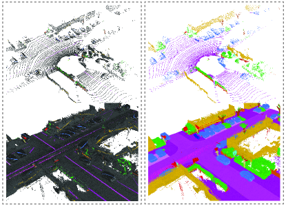
We provide scribble-annotations for the train-split of SemanticKITTI [5] for 19 classes. The resulting scribble-annotated data, which we call ScribbleKITTI, contains 189 million labeled points corresponding to 8.06% of the total point count. Fig. 1 shows an example from ScribbleKITTI.
Furthermore, in this paper we develop a novel learning method for 3D semantic segmentation that directly exploits scribble annotated LiDAR data. Learning from scribble annotations provides a unique challenge as no supervision/regularization is available from unlabeled points, which form the majority of the training data. A performance gap between scribble-supervised and fully supervised training could be very large if no special methods are designed for the former. To tackle this issue, we introduce three stand-alone contributions that can be combined with any 3D LiDAR segmentation model: a teacher-student consistency loss on unlabeled points, a self-training scheme designed for outdoor LiDAR scenes, and a novel descriptor that improves pseudo-label quality.
Specifically, we first introduce a weak form of supervision from unlabeled points via a consistency loss. Secondly, we strengthen this supervision by fixing the confident predictions of our model on the unlabeled points and employing self-training with pseudo-labels. The standard self-training strategy is however very prone to confirmation bias due to the long-tailed distribution of classes inherent in autonomous driving scenes and the large variation of point density across different ranges inherent in LiDAR data. To combat these, we develop a class-range-balanced pseudo-labeling strategy to uniformly sample target labels across all classes and ranges. Finally, to improve the quality of our pseudo-labels, we augment the input point cloud by using a novel descriptor that provides each point with the semantic prior about its local surrounding at multiple resolutions.
In summary, our contributions are as follows:
-
•
We present ScribbleKITTI, the first scribble-annotated LiDAR semantic segmentation dataset.
-
•
We propose class-range-balanced self-training to combat the inherent bias towards dominant classes and close ranged dense regions in pseudo-labels.
-
•
We further improve the pseudo-labeling quality by augmenting the input point cloud with a pyramid local semantic-context descriptor.
-
•
Putting these two contributions along with the mean teacher framework, our scribble-based pipeline achieves up to relative performance of fully supervised training while using only labeled points.
Our contributions remain orthogonal to the development of better neural network architectures and can be combined with any 3D LiDAR segmentation model.
2 Related Work
LiDAR Semantic Segmentation: As point clouds are irregular geometric data structures, current literature for 3D semantic segmentation mainly focuses on identifying and understanding various representation strategies amongst: operating directly on point coordinates [35, 36, 17, 44, 45, 20], projecting the LiDAR scene onto images and employ 2D architectures [30, 47, 48, 50, 12, 3], utilizing sparse 3D voxel grids [41, 11, 57, 25, 53], or utilizing multiple representations [51, 55, 2]. All of these models are developed under the fully-supervised framework, which requires densely annotated LiDAR point clouds that are time-consuming and tedious to acquire. In this work, our focus is different and our contributions are complementary. Our developed pipeline can be used with any such network in order to reduce the performance gap between fully-supervised and scribble-supervised training.
2D Scribble-supervised Semantic Segmentation: To alleviate the strenuous task of dense data annotation, two training methods can be used: weakly-supervised [32, 24, 22, 21, 29, 37], where only a subset of points are labeled on every frame, and semi-supervised [13, 33, 16, 23], where only a subset of frames are labeled within the dataset. Scribbles have been adopted as a user-friendly form of weak supervision [24]. The common approach when dealing with such weak annotations is to either employ online labeling through a consistency check using mean teacher [43, 26, 54, 9, 40], or to employ a self-training scheme where data is iteratively processed by generating offline target pseudo-labels and retraining [24, 7, 22, 38]. However, the naive approach of self-training on all predictions can introduce confirmation bias [4]. To combat this, threshold-based filtering can help reduce possible errors by only sampling confident predictions [8, 49, 58]. When facing long tailed distributions, CB-ST [59] uses class-balanced sampling to avoid the domination of head classes in the pseudo labels. DARS [16] extends CB-ST by re-distributing biased pseudo labels after thresholding. We extend the previously available methods to also include balancing against range to avoid undersampling points from distant, sparser regions of the LiDAR point cloud.
Incomplete Supervision in 3D Semantic Segmentation: In contrast to 2D, incomplete supervision for point clouds have remained underexplored. When tackling semi-supervised segmentation on LiDAR point clouds, Semi-sup [18] implements a pseudo-label guided point contrastive loss to extend supervision to unlabeled frames. Li et al. [23] and SSPC [10] employ self-training to achieve the same goal. Xu et al. [52] compares semi-supervised training to weakly-supervised on point clouds and argues that under a fixed labelling budget, weak supervision performs better for semantic segmentation. PSD [56] uses consistency check across perturbed branches to utilize unlabeled points in weakly supervised learning. However, the weak labels from existing methods [52, 56] are generated through offline uniform sampling from dense annotations which cannot be easily adopted during the dense labeling itself. In this work, we tackle a form of weakly-supervised segmentation based on line-scribbles. Instead of using simulated weak labels, we provide a human annotated dataset to realistically validate our method. Compared to uniform sampled labels, scribbles vitally do not provide any information on class boundaries and appear only in scribble-clusters, i.e. are much less spatially distributed within a scene.
3 The ScribbleKITTI Dataset
While LiDAR point cloud semantic segmentation has gained popularity over the past years, the number of large-scale datasets still remains low due to the complexity and time consumption of the data annotation process. Inspired by 2D scribble annotations [24] that are efficient and easy to generate, we propose using line-scribbles to annotate LiDAR point clouds for semantic segmentation and release ScribbleKITTI, the first scribble-annotated LiDAR point cloud dataset.
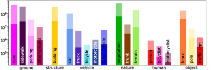
We annotate the train-split of SemanticKITTI [5] based on KITTI [15] which consists of 10 sequences, 19130 scans, 2349 million points. ScribbleKITTI contains 189 million labeled points corresponding to only 8.06% of the total point count. We choose SemanticKITTI for its current wide use and established benchmark. We retain the same 19 classes to encourage easy transitioning towards research into scribble-supervised LiDAR semantic segmentation. The class-wise label distribution is visualized in Fig. 2.
When annotating, we use line-scribbles rather than free-forming scribbles. LiDAR point clouds preserve the metric space and therefore things (e.g. car, truck) and stuff (e.g. terrain, road) mostly follow highly geometric structures. While both drawings are valid approaches, we found that line scribbles allow faster labeling of such geometric classes that span large distances (e.g. roads, sidewalks, buildings, fences), as annotators only need to provide two clicks (start and end) to annotate an entire segment. We illustrate this by showcasing an example annotated tile in Fig. 3.
Data Annotation: We use the help of student annotators. Following Behley et al. [5], we initially screen the annotators until they are comfortable navigating within the 3D space to ensure good results. We subdivide a sequence of superimposed point clouds into 100m by 100m tiles and label on a per-tile basis. We generate scribble annotations through line drawings using an adapted point labeling tool111https://github.com/jbehley/point_labeler, MIT License [5]. We overlap neighboring tiles to allow labeling consistency across the entire sequence. Finally, we do a comparison to SemanticKITTI to stay consistent with their class definitions. We provide further information in the supplementary materials on the labeling process.

4 Scribble-Supervised LiDAR Segmentation
The naive approach of tackling scribble-supervised semantic segmentation is to treat the problem similarly to any fully supervised task and employ a loss (typically cross-entropy) on the available labeled points.
We define a LiDAR point cloud as the set of points with denoting the 3D coordinates and the reflectance intensity. We further define as the set of labeled points. The objective function over frames can therefore be formulated as:
| (1) |
with denoting the predicted class distribution for the point of frame given the network parameters , and denoting the ground truth label.
In this baseline approach the unlabeled points which contain vital boundary information are not used. Furthermore due to the sheer lack of labeled data points, performance degradation is unavoidable, as confidence on long tailed object classes suffer due to the reduced supervision.
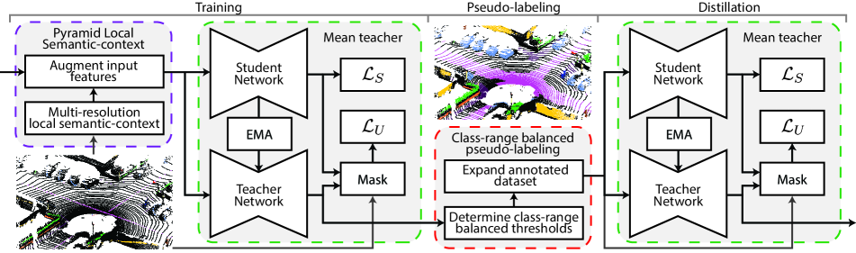
In the following sections, we address these issues by introducing three stand-alone methods that utilize unlabeled points and expand the annotated dataset: partial consistency loss with mean teacher (Sec. 4.1), class-range-balanced self-training (Sec. 4.2), and pyramid local semantic-context (Sec. 4.3). Our overall pipeline can be seen in Fig. 4.
4.1 Partial Consistency Loss with Mean Teacher
Firstly, we introduce further weak supervision to the unlabeled set of points via a consistency loss applied using mean teacher. The mean teacher framework is formed of two models, namely the student, parametrized by , and the teacher, parametrized by [43]. Unlike the student network, which is traditionally trained using gradient descent, the teacher weights are computed as the exponential moving average (EMA) of successive student weights, resulting in the update function:
| (2) |
for time step , with denoting the smoothing coefficient which determines the update speed. Stochastic averaging of weights has been shown to yield more accurate models than using the final training weights directly [34, 43], allowing the teacher predictions to be used as a form of weak supervision for the student under varying small perturbations.
We further define as the set of unlabeled points, i.e. . We introduce a consistency loss between the student and teacher networks, but unlike Tan et al. [40], we restrict the consistency loss to only unlabeled points . This allows a sharper supervision on labeled points in by eliminating the teacher injected uncertainties, while retaining the unlabeled supervision that takes advantage of the more accurate teacher predictions. This restriction is more in alignment with the applications of the mean teacher framework in semi-supervised tasks [43, 19, 46].
We extend our objective function (Eq. 1) to include supervision on unlabeled points as:
| (3) |
with denoting the predicted class distribution for the point given the network parameters , denoting the ground truth label. To reduce the Shannon mutual information, i.e. to increase the training signal from the consistency loss, we apply a heavier augmentation the student input in the form of global rotation, translation, random flip and white Gaussian noise [39, 6, 28].
While mean teacher introduces supervision on unlabeled points, the information gain is limited by the teachers performance. Even if the teacher predicts the correct label for a point, due to the soft pseudo-labeling, the confidences on other classes will continue to guide the student’s output.
4.2 Class-range-balanced Self-training (CRB-ST)
To combat this uncertainty injection and more directly utilize the confident predictions of unlabeled points, we expand the annotated dataset and employ self-training. Our goal by introducing self-training alongside mean teacher, is to keep the soft pseudo-label guidance of the mean teacher for uncertain predictions while hardening the pseudo-labels of certain predictions. Using the teacher’s most confident predictions, we generate target labels for a subset of unlabeled points. We define this set of pseudo-labeled points as and later retrain our network on .
Formally, we extend our objective function (Eq. 3) to also learn target labels as hidden variables:
| (4) |
where is the pseudo-label vector, denoting a one-shot vector, denoting the number of classes and denoting the negative log-confidence threshold. The generated pseudo-label set is given by . To exploit the increased performance generated from stochastic weight averaging, we sample labels from the teacher’s output ().
We initialize the optimization of Eq. 4 by setting the latent variable for all points, i.e. by only selecting the scribble-annotation (). The self-training protocol from pseudo-labels can then be summarised in two steps:
-
1.
Training: We fix and optimize the objective function with respect to .
-
2.
Pseudo-labeling: We fix (and effectively ) and optimize the objective function with respect to . We update given .
The two steps can be repeated to take advantage of the improved representation capability of the model through pseudo-labeling.
While self-training with pseudo-labels has been proven to be an effective strategy in scribble-supervised semantic segmentation [24, 38], the class distribution in autonomous driving scenes are inherently long tailed, which may result in the gradual dominance of large and easy-to-learn classes on generated pseudo-labels. CB-ST [59] proposes to sample labels while retaining the overall class distribution by setting thresholds in a class-wise manner. While this is sufficient in the 2D setting, we observe that 3D LiDAR data presents an additional unique challenge.
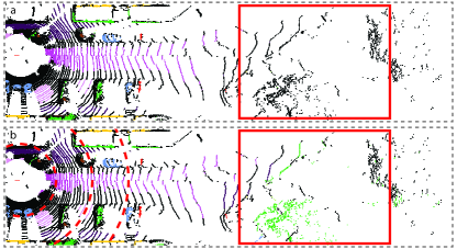
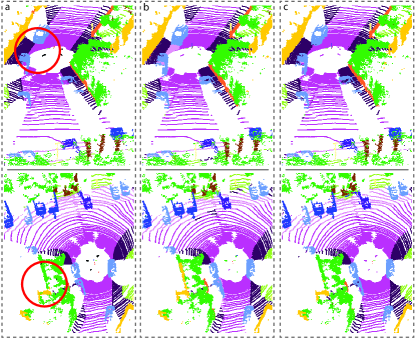
Due to the nature of the LiDAR sensor, the local point density varies based on the beam radius, as sparsity increases with distance. This results in sampling of pseudo-labels mainly from denser regions, which tend to show a higher estimation confidence. To reduce this bias in the pseudo-label generation, we propose a revised self-training scheme that not only balances based on the overall class-wise distribution, but also on range. We call our method class-range-balanced (CRB) pseudo-labeling and provide a visual sample in Fig. 5 comparing it to CB-ST.
We initially coarsely divide the transverse plane into annuli of width centered around the ego-vehicle. In Fig. 5.b we illustrate the first three in red dashed lines. Each annulus contains points that fall between a range of distances, from which we pseudo-label the globally highest confident predictions on a per-class basis. This ensures that we obtain reliable labels while distributing them proportionally across varying ranges and across all classes.
We redefine the self-training objective function (Eq.4) to include CRB as:
| (5) |
with denoting the negative log-threshold for a class-annulus pairing. To solve the nonlinear integer optimization task, we employ the following solver:
| (6) |
When determining , we take the maximum output probability of each point, i.e. the networks confidence for the predicted label, and store the confidence values of all points in all frames for each class-annulus pairing in a global vector. Each vector is then sorted in descending order. We define a hyperparameter which determines the percentage of pseudo-labels to be sampled, and find a threshold confidence for each vector by taking the value at index times the vectors length. is set as the negative logarithm of the threshold confidence. The process is summarized in Algorithm 1.
4.3 Pyramid Local Semantic-context (PLS)
With self-training, the performance of the final network (Sec. 4.2, training) is highly reliant on the pseudo-label quality. To ensure higher quality pseudo-labels, we further introduce a novel descriptor to enrich the features of the initial points by utilizing available scribbles.
We make the following two observations for the distribution of semantic classes in 3D space: (1) There exists a spatial smoothness constraint, i.e. a point in space is likely have the same class label as at least one of its neighbors since objects have nonzero dimensions; (2) There exists a semantic pattern constraint, i.e. a set of complex high-level rules governing inter-class spatial relations. For example, in outdoor autonomous driving scenes, vehicles lie on ground classes such as roads and parking areas, pedestrians often appear on sidewalks, buildings and vegetation outline roads.

We therefore argue that a local semantic prior can be used as a rich point descriptor to encapsulate the two stated cues. We propose using local semantic-context at scaling resolutions to reduce the ambiguity when propagating information between the labeled-unlabeled point sets and to improve pseudo-labeling quality. We identify that the distribution of class labels over global coordinates is a robust, compact semantic descriptor, especially for unlabeled points.
We initially discretize the space into coarse voxels. This step is crucial as to avoid over-descriptive features that cause the network to overfit to the scribble annotations, reducing its capability to generalize well and understand meaningful geometric relations. We use multiple sizes of bins in cylindrical coordinates in order to follow the inherent point distribution of the LiDAR sensor at different resolutions. For each bin we compute a coarse histogram:
| (7) |
as illustrated in Fig. 6. The pyramid local semantic-context (PLS) of all points is then defined as the concatenation of the normalized histograms:
| (8) |
for resolutions. We append PLS to the input features and redefine the input LiDAR point cloud as the augmented set of points . When optimizing Eq. 5, during the training step (Sec. 4.2) we substitute with such that we generate better quality pseudo-labels during pseudo-labeling.
At the end of the self-training pipeline, we require one extra distillation stage because PLS augmentation cannot be used during test-time as the scribble-information is not available. During distillation, we again set the input point cloud to . The resulting three stages of the overall pipeline is illustrated in Fig. 4.
5 Experiments
We carry out our experiments using Cylinder3D [57] but forego the applied test-time-augmentation (TTA) and test the performance on the fully annotated SemanticKITTI [5] valid-set unless stated otherwise. Alongside the mean-Intersection-over-Union (mIoU), we also provide the relative performance of scribble-supervised (SS) training to the fully supervised upper-bound (FS) in percentages (SS/FS).
Implementation Details: For MT we set . For CRB, we define annuli. For PLS, we divide into , and voxels. We only apply one iteration of self-training () as we don’t observe a significant increase in performance in consecutive steps.
5.1 Results
| Model | Supervision | Ours | mIoU | SS/FF |
car |
bicycle |
motorcycle |
truck |
other vehicle |
person |
bicyclist |
motorcyclist |
road |
parking |
sidewalk |
other ground |
building |
fence |
vegetation |
trunk |
terrain |
pole |
traffic sign |
|---|---|---|---|---|---|---|---|---|---|---|---|---|---|---|---|---|---|---|---|---|---|---|---|
| fully | 64.3 | - | 96.3 | 49.8 | 69.4 | 84.3 | 50.6 | 71.9 | 88.0 | 0.0 | 94.4 | 39.4 | 80.9 | 0.1 | 90.5 | 58.9 | 88.1 | 68.1 | 75.5 | 63.2 | 50.2 | ||
| Cylinder3D [57] | scribble | 57.0 | 88.6 | 88.5 | 39.9 | 58.0 | 58.4 | 48.1 | 68.6 | 77.0 | 0.5 | 84.4 | 30.4 | 72.2 | 2.5 | 89.4 | 48.4 | 81.9 | 64.6 | 59.8 | 61.2 | 48.7 | |
| scribble | ✓ | 61.3 | 95.3 | 91.0 | 41.1 | 58.1 | 85.5 | 57.1 | 71.7 | 80.9 | 0.0 | 87.2 | 35.1 | 74.6 | 3.3 | 88.8 | 51.5 | 86.3 | 68.0 | 70.7 | 63.4 | 49.5 | |
| fully | 61.1 | - | 95.7 | 20.4 | 63.9 | 70.3 | 45.5 | 65.0 | 78.5 | 0.0 | 93.5 | 49.6 | 81.0 | 0.2 | 91.1 | 63.8 | 87.2 | 68.5 | 72.3 | 64.4 | 49.1 | ||
| MinkowskiNet [11] | scribble | 55.0 | 90.0 | 88.1 | 13.2 | 55.1 | 72.3 | 36.9 | 61.3 | 77.1 | 0.0 | 83.4 | 32.7 | 71.0 | 0.3 | 90.0 | 50.0 | 84.1 | 66.6 | 65.8 | 61.6 | 35.2 | |
| scribble | ✓ | 58.5 | 95.7 | 91.1 | 23.8 | 59.0 | 66.3 | 58.6 | 65.2 | 75.2 | 0.0 | 83.8 | 36.1 | 72.4 | 0.7 | 90.2 | 51.8 | 86.7 | 68.5 | 72.5 | 62.5 | 46.6 | |
| fully | 63.8 | - | 97.1 | 35.2 | 64.6 | 72.7 | 64.3 | 69.7 | 82.5 | 0.2 | 93.5 | 50.8 | 81.0 | 0.3 | 91.1 | 63.5 | 89.2 | 66.1 | 77.2 | 64.1 | 49.4 | ||
| SPVCNN [41] | scribble | 56.9 | 89.2 | 88.6 | 25.7 | 55.9 | 67.4 | 48.8 | 65.0 | 78.2 | 0.0 | 82.6 | 30.4 | 70.1 | 0.3 | 90.5 | 49.6 | 84.4 | 67.6 | 66.1 | 61.6 | 48.7 | |
| scribble | ✓ | 60.8 | 95.3 | 91.1 | 35.3 | 57.2 | 71.1 | 63.8 | 70.0 | 81.3 | 0.0 | 84.6 | 37.9 | 72.9 | 0.0 | 90.0 | 54.0 | 87.4 | 71.1 | 73.0 | 64.0 | 50.5 |
We present the 3D semantic segmentation results from the SemanticKITTI -set in Tab. 1 for three state-of-the-art networks (Cylinder3D [57], MinkowskiNet [11], SPVCNN [41]) to demonstrate the model independence of our approach. For the training schedule and architecture details, please refer to the respective publications. In Fig. 7 we present visual results using Cylinder3D.
Due to the lack of available supervision, the three presented models trained on scribble-annotations show a relative performances (SS/FS) of , and compared to their respective fully supervised upper-bound. While the reduction in the number of supervised points reduce the class-wise performance across the board, this effect is further amplified for long tailed classes such as bicycle, truck and other-vehicle.
By applying our proposed pipeline for scribble-supervised LiDAR semantic segmentation, we are able to reduce the gap between the two training strategies significantly, reaching , , relative performance for all three models. As observed, the major performance gains originate from the same long tailed classes that initially show a deficit against their respective baselines.
5.2 Ablation Studies
| Labeled | Unlabeled | Valid | ||
| Model | Volume | Type | Used | mIoU |
| Cylinder3D [57] | 10% frames | fully | 46.8 | |
| Cylinder3D [57] | 8% points | scribbles | 57.0 | |
| Sup-only [18] | 10% frames | fully | 43.9 | |
| Sup-only [18] | 8% points | scribbles | 55.0 | |
| Semi-sup [18] | 10% frames | fully | ✓ | 49.9 |
| Sup-only+Ours | 8% points | scribbles | ✓ | 58.5 |
| Method | Train | Valid | ||||
|---|---|---|---|---|---|---|
| Baseline | MT | CRB-ST | PLS | mIoU | mIoU | SS/FS |
| ✓ | 77.6 | 57.0 | 88.6 | |||
| ✓ | ✓ | 78.0 | 59.3 | 92.2 | ||
| ✓ | ✓ | ✓ | - | 60.6 | 94.2 | |
| ✓ | ✓ | ✓ | 86.0 | - | - | |
| ✓ | ✓ | ✓ | ✓ | - | 61.3 | 95.3 |
Scribbles as Annotations: We compare our proposed labeling strategy of weakly labeling all frames to fully labeling partial frames under a fixed labeling budget in Tab. 2 and present the results for both Cylinder3D [57] and Sup-only, the baseline U-Net model employed in Semi-sup [18]. As seen, both models perform significantly better using scribble annotations compared to having full annotations on of the train-set by up to and mIoU.
Furthermore in Tab. 2, we also compare the current state-of-the-art on semi-supervised LiDAR semantic segmentation with our proposed scribble-supervised approach. Semi-sup [18] which further makes use of the unlabeled frames still shows a lower mIoU performance than a its baseline Semi-sup trained on scribble-annotations. Moreover, the same baseline model trained with our proposed pipeline further increases the gap to .
Effects of Network Components: We perform ablation studies to investigate the effects of the different components of our proposed pipeline for scribble-supervised LiDAR semantic segmentation. We report the performance on the SemanticKITTI -set for intermediate steps, as this metric provides an indication of the pseudo-labeling quality, and on the -set to assess the performance benefits of each individual component.
As seen in Tab. 3, by adding a weak form of supervision to the unlabeled point set via MT, we observe a increase in mIoU, which alone reduces the relative performance drop of scribble-supervised training below . However the fully labeled training performance does not increase significantly. Applying CRB-ST at this point yields an mIoU of . Using PLS, we can further increase the training mIoU by , which has the benefit of boosting pseudo-labeling accuracy from to and improving mIoU performance in the subsequent step of the self-training protocol. Self-training with CRB pseudo-labeling now yields a further increase in mIoU.
Pseudo-label Filtering for Self-training: We perform further ablation studies on the pseudo-labeling strategy used in the proposed self-training (ST) protocol and report the results in Tab. 4. We replace our proposed CRB pseudo-labeling module with naive sampling (where all predictions are taken as pseudo-labels), threshold-based sampling [8, 49, 58], class-balanced sampling (CB) [59] and DARS [16]. For all given strategies we use the same input predictions generated from the PLS augmented MT.
Due to the long-tailed nature of outdoor LiDAR scenes for semantic segmentation, CB and DARS show great improvements over naive and threshold based sampling strategies with improvements of up to . Here we observe that in 3D semantic segmentation, the confidence overlapping is not as prevalent as in 2D. Applying DARS on CB generated pseudo-labels results in a reduction of only data points on the entire train-set with (at most for head classes). Therefore both CB and DARS perform similarly at on the valid-set. After applying further balancing on range with our proposed CRB, we observe an improvement of over CB, reaching a relative performance of to fully-supervised.
| Labeling | Valid | |||
|---|---|---|---|---|
| Pseudo-labeling Method | Acc | mIoU | SS/FS | |
| Naive | - | 86.3 | 59.4 | 92.4 |
| Threshold-based [8, 49, 58] | 50% | 99.0 | 59.1 | 91.9 |
| Class-balanced [59] | 50% | 99.4 | 60.8 | 94.6 |
| DARS [16] | 50% | 99.3 | 60.8 | 94.6 |
| CRB (Ours) | 50% | 99.0 | 61.3 | 95.3 |
| Scribble | CRB-PL (50%) | |||
|---|---|---|---|---|
| Consistency-loss | mIoU | SS/FS | mIoU | SS/FS |
| All points [52] | 59.1 | 91.9 | 60.4 | 93.9 |
| Partial (Ours) | 59.3 | 92.2 | 61.3 | 95.3 |
Consistency-loss within Mean Teacher: We perform further ablation studies on the consistency loss within the mean teacher framework and compare our partial application on unlabeled points to the application on all points [52].
As seen in Tab. 5, the difference between the two losses is negligible when training with scribble annotations. Scribbles only account for roughly of the total point count, therefore the loss is mainly dominated by the unsupervised points in either setting. However, when training on generated pseudo-labels, we observe that the teacher network can inject uncertainties to labeled points, weakening the introduced supervision from the pseudo-labels and causing a decrease in mIoU of .
6 Conclusion
We have presented a weakly-supervised pipeline for LiDAR semantic segmentation based on scribble annotations. Our pipeline comprises of three stand-alone contributions that can be combined with any LiDAR semantic segmentation model to reduce the gap between fully-supervised and scribble-supervised training.
Limitations: We only annotate the train-split of SemanticKITTI [5]. We haven’t applied our method to different datasets and LiDAR sensors due to annotation cost.
Acknowledgements: Special thanks to Zeynep Demirkol and Tim Brödermann for their efforts during annotation.
References
- [1] Jiwoon Ahn and Suha Kwak. Learning pixel-level semantic affinity with image-level supervision for weakly supervised semantic segmentation. In Proceedings of the IEEE Conference on Computer Vision and Pattern Recognition (CVPR), June 2018.
- [2] Yara Ali Alnaggar, Mohamed Afifi, Karim Amer, and Mohamed ElHelw. Multi projection fusion for real-time semantic segmentation of 3d lidar point clouds. In Proceedings of the IEEE/CVF Winter Conference on Applications of Computer Vision, pages 1800–1809, 2021.
- [3] Inigo Alonso, Luis Riazuelo, Luis Montesano, and Ana C Murillo. 3d-mininet: Learning a 2d representation from point clouds for fast and efficient 3d lidar semantic segmentation. IEEE Robotics and Automation Letters, 5(4):5432–5439, 2020.
- [4] Eric Arazo, Diego Ortego, Paul Albert, Noel E O’Connor, and Kevin McGuinness. Pseudo-labeling and confirmation bias in deep semi-supervised learning. In 2020 International Joint Conference on Neural Networks (IJCNN), pages 1–8. IEEE, 2020.
- [5] Jens Behley, Martin Garbade, Andres Milioto, Jan Quenzel, Sven Behnke, Cyrill Stachniss, and Jurgen Gall. Semantickitti: A dataset for semantic scene understanding of lidar sequences. In Proceedings of the IEEE/CVF International Conference on Computer Vision, pages 9297–9307, 2019.
- [6] David Berthelot, Nicholas Carlini, Ian Goodfellow, Nicolas Papernot, Avital Oliver, and Colin Raffel. Mixmatch: A holistic approach to semi-supervised learning. arXiv preprint arXiv:1905.02249, 2019.
- [7] Yigit B Can, Krishna Chaitanya, Basil Mustafa, Lisa M Koch, Ender Konukoglu, and Christian F Baumgartner. Learning to segment medical images with scribble-supervision alone. In Deep Learning in Medical Image Analysis and Multimodal Learning for Clinical Decision Support, pages 236–244. Springer, 2018.
- [8] Paola Cascante-Bonilla, Fuwen Tan, Yanjun Qi, and Vicente Ordonez. Curriculum labeling: Revisiting pseudo-labeling for semi-supervised learning. arXiv preprint arXiv:2001.06001, 2020.
- [9] Hongjun Chen, Jinbao Wang, Hong Cai Chen, Xiantong Zhen, Feng Zheng, Rongrong Ji, and Ling Shao. Seminar learning for click-level weakly supervised semantic segmentation. In Proceedings of the IEEE/CVF International Conference on Computer Vision (ICCV), pages 6920–6929, October 2021.
- [10] Mingmei Cheng, Le Hui, Jin Xie, and Jian Yang. Sspc-net: Semi-supervised semantic 3d point cloud segmentation network. arXiv preprint arXiv:2104.07861, 2021.
- [11] Christopher Choy, JunYoung Gwak, and Silvio Savarese. 4d spatio-temporal convnets: Minkowski convolutional neural networks. In Proceedings of the IEEE/CVF Conference on Computer Vision and Pattern Recognition, pages 3075–3084, 2019.
- [12] Tiago Cortinhal, George Tzelepis, and Eren Erdal Aksoy. Salsanext: Fast, uncertainty-aware semantic segmentation of lidar point clouds. In International Symposium on Visual Computing, pages 207–222. Springer, 2020.
- [13] Wenhui Cui, Yanlin Liu, Yuxing Li, Menghao Guo, Yiming Li, Xiuli Li, Tianle Wang, Xiangzhu Zeng, and Chuyang Ye. Semi-supervised brain lesion segmentation with an adapted mean teacher model. In International Conference on Information Processing in Medical Imaging, pages 554–565. Springer, 2019.
- [14] Jifeng Dai, Kaiming He, and Jian Sun. Boxsup: Exploiting bounding boxes to supervise convolutional networks for semantic segmentation. In Proceedings of the IEEE international conference on computer vision, pages 1635–1643, 2015.
- [15] Andreas Geiger, Philip Lenz, Christoph Stiller, and Raquel Urtasun. Vision meets robotics: The kitti dataset. The International Journal of Robotics Research, 32(11):1231–1237, 2013.
- [16] Ruifei He, Jihan Yang, and Xiaojuan Qi. Re-distributing biased pseudo labels for semi-supervised semantic segmentation: A baseline investigation. In Proceedings of the IEEE/CVF International Conference on Computer Vision, pages 6930–6940, 2021.
- [17] Qingyong Hu, Bo Yang, Linhai Xie, Stefano Rosa, Yulan Guo, Zhihua Wang, Niki Trigoni, and Andrew Markham. Randla-net: Efficient semantic segmentation of large-scale point clouds. In Proceedings of the IEEE/CVF Conference on Computer Vision and Pattern Recognition, pages 11108–11117, 2020.
- [18] Li Jiang, Shaoshuai Shi, Zhuotao Tian, Xin Lai, Shu Liu, Chi-Wing Fu, and Jiaya Jia. Guided point contrastive learning for semi-supervised point cloud semantic segmentation. In Proceedings of the IEEE/CVF International Conference on Computer Vision (ICCV), pages 6423–6432, October 2021.
- [19] Jongmok Kim, Jooyoung Jang, and Hyunwoo Park. Structured consistency loss for semi-supervised semantic segmentation. arXiv preprint arXiv:2001.04647, 2020.
- [20] Deyvid Kochanov, Fatemeh Karimi Nejadasl, and Olaf Booij. Kprnet: Improving projection-based lidar semantic segmentation. arXiv preprint arXiv:2007.12668, 2020.
- [21] Alexander Kolesnikov and Christoph H Lampert. Seed, expand and constrain: Three principles for weakly-supervised image segmentation. In European conference on computer vision, pages 695–711. Springer, 2016.
- [22] Hyeonsoo Lee and Won-Ki Jeong. Scribble2label: Scribble-supervised cell segmentation via self-generating pseudo-labels with consistency. In International Conference on Medical Image Computing and Computer-Assisted Intervention, pages 14–23. Springer, 2020.
- [23] Hongyan Li, Zhengxing Sun, Yunjie Wu, and Youcheng Song. Semi-supervised point cloud segmentation using self-training with label confidence prediction. Neurocomputing, 437:227–237, 2021.
- [24] Di Lin, Jifeng Dai, Jiaya Jia, Kaiming He, and Jian Sun. Scribblesup: Scribble-supervised convolutional networks for semantic segmentation. In Proceedings of the IEEE conference on computer vision and pattern recognition, pages 3159–3167, 2016.
- [25] Venice Erin Liong, Thi Ngoc Tho Nguyen, Sergi Widjaja, Dhananjai Sharma, and Zhuang Jie Chong. Amvnet: Assertion-based multi-view fusion network for lidar semantic segmentation. arXiv preprint arXiv:2012.04934, 2020.
- [26] Xiaoming Liu, Quan Yuan, Yaozong Gao, Kelei He, Shuo Wang, Xiao Tang, Jinshan Tang, and Dinggang Shen. Weakly supervised segmentation of covid19 infection with scribble annotation on ct images. Pattern recognition, 122:108341, 2022.
- [27] Yen-Cheng Liu, Chih-Yao Ma, Zijian He, Chia-Wen Kuo, Kan Chen, Peizhao Zhang, Bichen Wu, Zsolt Kira, and Peter Vajda. Unbiased teacher for semi-supervised object detection. arXiv preprint arXiv:2102.09480, 2021.
- [28] Luke Melas-Kyriazi and Arjun K Manrai. Pixmatch: Unsupervised domain adaptation via pixelwise consistency training. In Proceedings of the IEEE/CVF Conference on Computer Vision and Pattern Recognition, pages 12435–12445, 2021.
- [29] Qinghao Meng, Wenguan Wang, Tianfei Zhou, Jianbing Shen, Luc Van Gool, and Dengxin Dai. Weakly supervised 3d object detection from lidar point cloud. In European Conference on Computer Vision (ECCV), 2020.
- [30] Andres Milioto, Ignacio Vizzo, Jens Behley, and Cyrill Stachniss. Rangenet++: Fast and accurate lidar semantic segmentation. In 2019 IEEE/RSJ International Conference on Intelligent Robots and Systems (IROS), pages 4213–4220. IEEE, 2019.
- [31] G Papandreou, LC Chen, K Murphy, and AL Yuille. Weakly-and semi-supervised learning of a dcnn for semantic image segmentation. arxiv 2015. arXiv preprint arXiv:1502.02734.
- [32] Deepak Pathak, Philipp Krahenbuhl, and Trevor Darrell. Constrained convolutional neural networks for weakly supervised segmentation. In Proceedings of the IEEE international conference on computer vision, pages 1796–1804, 2015.
- [33] Christian S Perone and Julien Cohen-Adad. Deep semi-supervised segmentation with weight-averaged consistency targets. In Deep learning in medical image analysis and multimodal learning for clinical decision support, pages 12–19. Springer, 2018.
- [34] Boris T Polyak and Anatoli B Juditsky. Acceleration of stochastic approximation by averaging. SIAM journal on control and optimization, 30(4):838–855, 1992.
- [35] Charles R Qi, Hao Su, Kaichun Mo, and Leonidas J Guibas. Pointnet: Deep learning on point sets for 3d classification and segmentation. In Proceedings of the IEEE conference on computer vision and pattern recognition, pages 652–660, 2017.
- [36] Charles R Qi, Li Yi, Hao Su, and Leonidas J Guibas. Pointnet++: Deep hierarchical feature learning on point sets in a metric space. arXiv preprint arXiv:1706.02413, 2017.
- [37] Ruobing Shen, Thomas Guthier, Hyundai Mobis, Bo Tang, and Ismail Ben Ayed. Scribble supervised annotation algorithms of panoptic segmentation for autonomous driving. In Proc. NeurIPS Workshop Mach. Learn. Auton. Driving, 2019.
- [38] Zhenyu Shu, Xiaoyong Shen, Shiqing Xin, Qingjun Chang, Jieqing Feng, Ladislav Kavan, and Ligang Liu. Scribble-based 3d shape segmentation via weakly-supervised learning. IEEE Transactions on Visualization and Computer Graphics, 26(8):2671–2682, 2020.
- [39] Kihyuk Sohn, David Berthelot, Chun-Liang Li, Zizhao Zhang, Nicholas Carlini, Ekin D Cubuk, Alex Kurakin, Han Zhang, and Colin Raffel. Fixmatch: Simplifying semi-supervised learning with consistency and confidence. arXiv preprint arXiv:2001.07685, 2020.
- [40] Li Tan, WenFeng Luo, and Meng Yang. Weakly-supervised semantic segmentation with mean teacher learning. In International Conference on Intelligent Science and Big Data Engineering, pages 324–335. Springer, 2019.
- [41] Haotian* Tang, Zhijian* Liu, Shengyu Zhao, Yujun Lin, Ji Lin, Hanrui Wang, and Song Han. Searching efficient 3d architectures with sparse point-voxel convolution. In European Conference on Computer Vision, 2020.
- [42] Meng Tang, Federico Perazzi, Abdelaziz Djelouah, Ismail Ben Ayed, Christopher Schroers, and Yuri Boykov. On regularized losses for weakly-supervised cnn segmentation. In Proceedings of the European Conference on Computer Vision (ECCV), pages 507–522, 2018.
- [43] Antti Tarvainen and Harri Valpola. Mean teachers are better role models: Weight-averaged consistency targets improve semi-supervised deep learning results. arXiv preprint arXiv:1703.01780, 2017.
- [44] Hugues Thomas, Charles R Qi, Jean-Emmanuel Deschaud, Beatriz Marcotegui, François Goulette, and Leonidas J Guibas. Kpconv: Flexible and deformable convolution for point clouds. In Proceedings of the IEEE/CVF International Conference on Computer Vision, pages 6411–6420, 2019.
- [45] Ozan Unal, Luc Van Gool, and Dengxin Dai. Improving point cloud semantic segmentation by learning 3d object detection. In Proceedings of the IEEE/CVF Winter Conference on Applications of Computer Vision, pages 2950–2959, 2021.
- [46] Xiang Wang, Shiwei Zhang, Zhiwu Qing, Yuanjie Shao, Changxin Gao, and Nong Sang. Self-supervised learning for semi-supervised temporal action proposal. In Proceedings of the IEEE/CVF Conference on Computer Vision and Pattern Recognition (CVPR), pages 1905–1914, June 2021.
- [47] Bichen Wu, Alvin Wan, Xiangyu Yue, and Kurt Keutzer. Squeezeseg: Convolutional neural nets with recurrent crf for real-time road-object segmentation from 3d lidar point cloud. In 2018 IEEE International Conference on Robotics and Automation (ICRA), pages 1887–1893. IEEE, 2018.
- [48] Bichen Wu, Xuanyu Zhou, Sicheng Zhao, Xiangyu Yue, and Kurt Keutzer. Squeezesegv2: Improved model structure and unsupervised domain adaptation for road-object segmentation from a lidar point cloud. In 2019 International Conference on Robotics and Automation (ICRA), pages 4376–4382. IEEE, 2019.
- [49] Qizhe Xie, Minh-Thang Luong, Eduard Hovy, and Quoc V Le. Self-training with noisy student improves imagenet classification. In Proceedings of the IEEE/CVF Conference on Computer Vision and Pattern Recognition, pages 10687–10698, 2020.
- [50] Chenfeng Xu, Bichen Wu, Zining Wang, Wei Zhan, Peter Vajda, Kurt Keutzer, and Masayoshi Tomizuka. Squeezesegv3: Spatially-adaptive convolution for efficient point-cloud segmentation. In European Conference on Computer Vision, pages 1–19. Springer, 2020.
- [51] Jianyun Xu, Ruixiang Zhang, Jian Dou, Yushi Zhu, Jie Sun, and Shiliang Pu. Rpvnet: A deep and efficient range-point-voxel fusion network for lidar point cloud segmentation. arXiv preprint arXiv:2103.12978, 2021.
- [52] Xun Xu and Gim Hee Lee. Weakly supervised semantic point cloud segmentation: Towards 10x fewer labels. In Proceedings of the IEEE/CVF Conference on Computer Vision and Pattern Recognition (CVPR), June 2020.
- [53] Xu Yan, Jiantao Gao, Jie Li, Ruimao Zhang, Zhen Li, Rui Huang, and Shuguang Cui. Sparse single sweep lidar point cloud segmentation via learning contextual shape priors from scene completion. arXiv preprint arXiv:2012.03762, 2020.
- [54] Dong Zhang, Bo Chen, Jaron Chong, and Shuo Li. Weakly-supervised teacher-student network for liver tumor segmentation from non-enhanced images. Medical Image Analysis, 70:102005, 2021.
- [55] Feihu Zhang, Jin Fang, Benjamin Wah, and Philip Torr. Deep fusionnet for point cloud semantic segmentation. In Computer Vision–ECCV 2020: 16th European Conference, Glasgow, UK, August 23–28, 2020, Proceedings, Part XXIV 16, pages 644–663. Springer, 2020.
- [56] Yachao Zhang, Yanyun Qu, Yuan Xie, Zonghao Li, Shanshan Zheng, and Cuihua Li. Perturbed self-distillation: Weakly supervised large-scale point cloud semantic segmentation. In Proceedings of the IEEE/CVF International Conference on Computer Vision (ICCV), pages 15520–15528, October 2021.
- [57] Xinge Zhu, Hui Zhou, Tai Wang, Fangzhou Hong, Yuexin Ma, Wei Li, Hongsheng Li, and Dahua Lin. Cylindrical and asymmetrical 3d convolution networks for lidar segmentation. arXiv preprint arXiv:2011.10033, 2020.
- [58] Barret Zoph, Golnaz Ghiasi, Tsung-Yi Lin, Yin Cui, Hanxiao Liu, Ekin D Cubuk, and Quoc V Le. Rethinking pre-training and self-training. arXiv preprint arXiv:2006.06882, 2020.
- [59] Yang Zou, Zhiding Yu, B.V.K. Vijaya Kumar, and Jinsong Wang. Unsupervised domain adaptation for semantic segmentation via class-balanced self-training. In Proceedings of the European Conference on Computer Vision (ECCV), September 2018.
7 Supplementary Material
7.1 The ScribbleKITTI Dataset
The goal of generating scribble-annotations is to to be fast and efficient while retaining as much information as possible to allow relatively high performance when compared to fully-supervised training. To this end, we formulate a set of guidelines for our annotators that also allows us to remain consistent across the dataset.
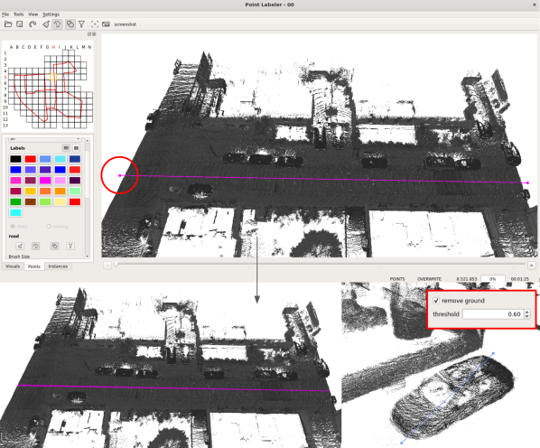
Process: We modify the point labeler [5] to include line annotations. An example of the labeler GUI can be seen in Fig. 8. As seen, the annotator draws lines on the LiDAR scene by determining its start and end points. The tool also allows multi-segment lines (when providing more than two points) to allow easier labeling of curved surfaces. As LiDAR point clouds are inherently sparse, we add a thickness to the drawn line. All points, who’s projections fall onto the thickened line, are labeled. At height we set the line thickness to pixels. We adjust the thickness proportionally to the zoom settings to remain consistent throughout the labeling.
Guidelines: During labeling, each object in a scene (e.g. vehicle, person, sign, trunk) is marked with a single line. To ease the process and eliminate any spillage to the ground points, the annotators can use a threshold based filter for the z-axis (which was already implemented in the point labeler [5]) to hide ground points. An example can be see in Fig. 8 bottom-right. However, unlike the dense annotated case, annotators do not need to later remove the filter in order to determine difficult border points between objects and ground classes.
For classes that cover large distances, e.g ground classes (e.g. road, sidewalk, parking) and structure façades (e.g. building, fence), we try to annotate each segment using the least amount of scribbles. For example, given a north-south facing road segment that later turns right, the annotator draws two line-scribbles: 1) a north-south facing scribble that extends from the tile edge to junction, and 2) a west-east facing scribble that extends from the junction to the corresponding tile edge. If object interfere with the line-scribble (e.g. a car is in the middle of the road) the annotator can chose to scribble on either side of the object. For vegetation, each patch of greenery is annotated once. When periodically placed trees or bushes have similar heights, the threshold based filter can be used to isolate them, allowing a single annotation line to cover multiple individual trees. This also holds for sparse vegetation clusters in empty space (see main text Fig. 3 - bottom right). As 2D lines are projected onto the 3D surface to generate annotations, such scribbles may become indistinguishable once the viewing angle changes.
7.2 Ablation Studies
Semi-supervised dataset: Our line-scribbles label roughly of the total point count and take of the time to acquire compared to their fully labeled counterpart (based on the reported times of SemanticKITTI [5]). Under a fixed labeling budget, we show that scribble-annotating all frames enables better representation capabilities compared to fully labeling partial frames (see main text Sec. 5.2). For these experiments, when simulating the semi-labeled setting, we follow the data generation process of Semi-sup [18] with labeling.
Labeling Percentage for CRB-ST: We further investigate the effect of the labeling percentage for CRB-ST. In Tab. 6 we compare results for three values at , , . As seen, the mIoU performance does depend on the percentage of predictions selected as pseudo-labels. outperforms and by and respectively, achieving a better balance between the introduction of more supervision through pseudo-labeling, and the reduction of errors propagating from pseudo-labeling to distillation.
| mIoU | SS/FS | |
|---|---|---|
| 30% | 60.9 | 94.7 |
| 50% | 61.3 | 95.3 |
| 70% | 60.8 | 94.6 |