Gravitational field of slightly deformed naked singularities

Abstract

We derive a particular approximate solution of Einstein equations, describing the gravitational field of a mass distribution that slightly deviates from spherical symmetry. The deviation is described by means of a quadrupole parameter that is responsible for the appearance of a curvature singularity, which is not covered by a horizon. We investigate the motion of test particles in the gravitational field of this naked singularity and show that the quadrupole parameter affects the properties of Schwarzschild trajectories. By investigating radial geodesics, we find that no effects of repulsive gravity are present. We interpreted this result as indicating that repulsive gravity is non-linear effect.

I Introduction

Although the existence of naked singularities in Nature is the subject of intense debate nowadays, it has been well established that Einstein field equations for the gravitational field allow solutions that can be interpreted as describing naked singularities. In particular, black hole solutions are characterized by the existence of naked singularity counterparts kerr . However, it seems that the particular choice of the physical parameters, which is necessary for the formation of naked singularities, is difficult to be realizable in Nature. Indeed, a rotating naked singularity needs a specific angular momentum that must be greater that its mass (in geometric units), a condition that probably cannot be fulfilled in realistic configurations because it would imply such a high angular velocity that the object would destroy itself before reaching it mtw .

There is, however, a simpler way to generate naked singularities, namely, by considering mass distributions with quadrupole moment quev11 . Indeed, from the point of view of multipole moments, the uniqueness theorems prove that black holes can have only mass monopole and angular momentum dipole heusler . Consequently, the addition of a quadrupole to a mass distribution, even in the static case, would imply that the corresponding gravitational field describes a naked singularity. Consequently, a simple shape deviation from spherical symmetry in a mass distribution leads to the appearance of naked singularities. In previous works quev11 ; Quevedo2016 ; Boshkayev2016 ; Boshkayevpxa , we used a particular static quadrupolar solution zipoy ; voorhees ; malafarina05 ; solutions to study the physical properties of naked singularities.

There are several solutions of Einstein field equations that can be used to describe the exterior gravitational field of a static mass distribution with quadrupole moment aqs18 . In the limiting case of vanishing quadrupole, they reduce to the spacetime of a Schwarzschild black hole. An interesting characteristic of all of them is that the outermost naked singularity is a sphere with radius $r=2m$, where $m$ is the mass of the gravitational source. This could be interpreted intuitively as if the presence of the quadrupole causes the destruction of the regular horizon turning it into a singular hypersurface.

In this work, we show that this is not always the case. Indeed, we will derive a new solution, whose singularity is located on a sphere of radius $r=m$. This means that in this case the quadrupole completely destroys the regular horizon at $r=2m$, but generates a new special hypersurface at $r=m$ which contains a singularity. To derive this new solution, we use the fact in realistic situations we expect that compact objects deviates only slightly from spherical symmetry. This implies that the quadrupole can be considered as a small quantity. With this in mind, we investigate a particular approximate line element, which is valid only up to the first order in the quadrupole parameter. Then, we find the general solution of the corresponding Einstein vacuum field equations and show that a particular solution is characterized by a curvature singularity located on a sphere of radius $r=m$.

This work is organized as follows. In Sec. II, we consider a line element that is especially adapted to the study of interior and exterior solutions. We derive the general field equations for the case of vacuum gravitational fields. In Sec. III, we find the most general solution that is linear in the quadrupole moment. We select a particular case that is characterized by the presence of naked singularity at a distance $r=m$ from the origin of coordinates. We also calculate the Newtonian limit of the new approximate solution and show that it corresponds to a mass distribution with a small quadrupole. In Sec. IV, we investigate the motion of test particles in the spacetime described by the approximate solution. In general, we find that the quadrupole affects the behavior of Schwarzschild orbits. By analyzing the behavior of free falling particles we show that no effects associated with the presence of repulsive gravity can be detected in contrast to repulsive effects found previously in the case of exact solutions with quadrupole. We conclude that repulsive gravity in naked singularities is a non-linear phenomenon. Finally, Sec. V contains a summary of our results.

II Line element and field equations

The search for and investigation of physically meaningful solutions of Einstein equations begins with the choice of an appropriate line element. In the case of static gravitational fields of deformed mass distributions, one can assume that the fields preserve axial symmetry. Moreover, if we are interested in describing the gravitational field outside as well as inside the mass distribution, it is convenient to choose a line element that can be used in both cases. In a previous work approxi_2021 , we found interior perfect-fluid solutions that can be matched with exterior vacuum solutions under the assumption that the quadrupole moment is small. From a physical point of view, this implies that the mass distribution is only slightly deformed. We were able to find a particular line element that can be used to search for interior and exterior approximate solutions. It can be written as

$$ds^{2}= e^{2\nu}(1+qa)dt^{2}-(1+qc+qb)\frac{dr^{2}}{1-\frac{2\tilde{m}}{r}}$$ (1)

$$-(1+qa+qb)r^{2}d\theta^{2}-(1-qa)r^{2}\sin^{2}\theta d\varphi^{2}\ ,$$

where the set of $(t,r,\theta,\varphi)$ can be interpreted as polar coordinates in the limiting case $q\rightarrow 0$. Moreover, the functions $\nu=\nu(r)$, $a=a(r)$, $c=c(r)$, $\tilde{m}=\tilde{m}(r)$, and $b=b(r,\theta)$ are arbitrary.

In the particular case $q=0$, the above line element can be used to describe the exterior Schwarzschild solution

$$\tilde{m}=m=const,\ e^{2\nu}=1-\frac{2m}{r}\ ,$$ (2)

and the interior perfect fluid Schwarzschild metric with

$$\tilde{m}=4\pi\rho R^{3}\ ,\ p=\frac{3m}{4\pi R^{3}}\frac{\left[f(r)-f(R)\right]}{\left[3f(R)-f(r)\right]}\ ,$$ (3)

with

$$e^{2\nu}=\bigg{[}\frac{3}{2}f\left(R\right)-\frac{1}{2}f\left(r\right)\bigg{]}^{2},\ \ f\left(r\right)=\sqrt{1-\frac{2mr^{2}}{R^{3}}}$$ (4)

where $\rho=const$ and $p=p(r)$ are the density and pressure of the fluid, respectively.

Furthermore, for $q\neq 0$ the line element (1) contains the approximate (up to the first order in $q$) quadrupolar metric ($q-$metric), which has been interpreted as the simplest generalization of the Schwarzschild metric that includes a quadrupole moment quev11 . In this limit, $q$ has been interpreted as the quadrupole parameter.

Here, we will use the advantages of the line element (1) to search for more general approximate solutions. Then, the Einstein vacuum field equations, up to the first order in $q$, can be written as

$$\tilde{m}_{,r}=0\quad{\rm i.e.}\quad\tilde{m}=m=const.\ ,$$ (5)

$$\nu_{,r}=\frac{{m}}{r\left(r-2{m}\right)}\ ,$$ (6)

$$(r-m)(a_{,r}-c_{,r})+(a-c)=0\ ,$$ (7)

$$2 r\left(r-2m\right)a_{,rr}+\left(3r-m\right)a_{,r}+\left(r-3m\right)c_{,r}$$ (8)

$$-2\left(a-c\right)=0,$$

$$r \left(r-2m\right)b_{,rr}+b_{,\theta\theta}+\left(r-m\right)b_{,r}-2\left(r-2m\right)c_{,r}$$ (9)

$$+2\left(a-c\right)=0,$$

$$\left(r^{2}-2mr+m^{2}\sin^{2}\theta\right)b_{,\theta}+2r\left(r-2m\right)$$

$$\times\left(ma_{,r}-a+c\right)\sin\theta\cos\theta=0,$$ (10)

$$\left(r^{2}-2mr+m^{2}\sin^{2}\theta\right)b_{,r}+2\left(r-2m\right)$$

$$\times\left(r-m\sin^{2}\theta\right)a_{,r}+2\left(r-m\right)\left(a-c\right)\sin^{2}\theta=0,$$ (11)

where a comma represents partial differentiation with respect to the corresponding coordinate. For simplicity, we replaced the solution of the first equation $\tilde{m}=m=const.$ in the remaining equations.

III Approximate solutions

We now investigate the system of partial differential equation (6)-(11). Equations (6) and (7) can be integrated and yield

$$\nu=\frac{1}{2}\ln\left(1-\frac{2m}{r}\right)+\alpha_{1}\ ,\quad a-c=\frac{\alpha_{2}m^{2}}{(r-m)^{2}}\ ,$$ (12)

where $\alpha_{1}$ and $\alpha_{2}$ are dimensionless integration constants. It turns out that the remaining system of partial differential equations can be integrated in general and yields

$$a=-\frac{\alpha_{2}m}{r-m}+\frac{1}{2}\left(\alpha_{3}-{\alpha_{2}}\right)\ln\left(1-\frac{2m}{r}\right)+\alpha_{4}\ ,$$ (13)

$$c=-\frac{\alpha_{2}mr}{(r-m)^{2}}+\frac{1}{2}\left(\alpha_{3}-{\alpha_{2}}\right)\ln\left(1-\frac{2m}{r}\right)+\alpha_{4}\ ,$$ (14)

$$b= \frac{2\alpha_{2}m}{r-m}-\left(\alpha_{3}-{\alpha_{2}}\right)\bigg{[}\ln 2$$ (15)

$$+ \ln\left(1-\frac{2m}{r}+\frac{m^{2}\sin^{2}\theta}{r^{2}}\right)\bigg{]}+\alpha_{5}\ ,$$

where $\alpha_{3}$, $\alpha_{4}$, and $\alpha_{5}$ are dimensionless integration constants. We can see that the general approximate exterior solution with quadrupole moment is represented by the 5-parameter family of solutions (12)–(15). In this general solution, the additive constants $\alpha_{4}$ and $\alpha_{5}$ can be chosen such that at infinity the solution describes the Minkowski spacetime in spherical coordinates. This means that non asymptotically flat solutions are also contained in the above general solution.

To partially investigate the physical meaning of this solution, we calculate the Kretschmann scalar $K=R_{abcd}R^{abcd}$. We obtain

$$K= \frac{48m^{2}}{r^{6}}\Bigg{\{}1+q\Bigg{[}\left(\alpha_{2}-\alpha_{3}\right)\Big{[}\ln\left(1-\frac{2m}{r}\right)$$ (16)

$$- 2\ln\left(1-\frac{2m}{r}+\frac{m^{2}}{r^{2}}\sin^{2}{\theta}\right)-2\ln 2\Big{]}$$

$$+\alpha_{2} A_{1}+\alpha_{3}A_{2}-2\left(\alpha_{4}+\alpha_{5}\right)+\alpha_{2}A_{3}\Bigg{]}+\mathcal{O}(q^{2})\Bigg{\}}$$

where

$$A_{1} = -\frac{1}{6\left(m^{2}\sin^{2}\theta-2mr+r^{2}\right)\left(m-r\right)^{3}m^{2}}$$ (17)

$$\times \bigg{[}\left(12m^{3}-11m^{2}r-14mr^{2}+11r^{3}\right)m^{4}\cos^{2}\theta$$

$$- \left(12m^{3}-17m^{2}r-2mr^{2}+5r^{3}\right)m^{2}\left(m-r\right)^{2}\bigg{]}$$

$$A_{2}=\frac{2m^{2}\sin^{2}\theta-3mr+r^{2}}{m^{2}\sin^{2}\theta-2mr+r^{2}}$$ (18)

$$A_{3}=-\frac{1}{6}\frac{r\big{[}7\left(m-r\right)^{2}-2r^{2}\big{]}}{\left(m-r\right)^{3}}$$ (19)

where the term proportional to $q^{2}$ has been neglected. We can see that this approximate spacetime is characterized by the presence of three different curvature singularities located at

$$r=0\ ,\quad r=m\,\quad r=2m\ ,\quad r=m(1\pm\cos\theta)\ .$$ (20)

The geometric structure of the curvature singularities of the solutions (12), (13), (14) and (15) is illustrated in Fig.1.

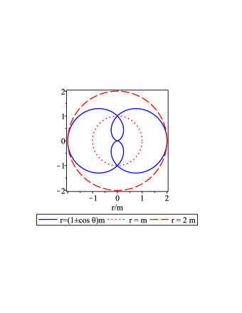
Figure 1: Curvature singularities of the general metric.

Another interesting particular case corresponds to the choice

$$\alpha_{1}=0\ ,\quad\alpha_{3}={\alpha_{2}}\ ,\quad\alpha_{4}=0\ ,\quad\alpha_{5}=0\ ,$$ (21)

which leads to the line element

$$ds^{2} = \left(1-\frac{2m}{r}\right)\left(1-\frac{q\alpha_{2}m}{r-m}\right)dt^{2}$$ (22)

$$-\left[1+\frac{q\alpha_{2}m(r-2m)}{(r-m)^{2}}\right]\frac{dr^{2}}{1-\frac{2m}{r}}$$

$$-\left(1+\frac{q\alpha_{2}m}{r-m}\right)r^{2}(d\theta^{2}+\sin^{2}\theta d\varphi^{2})\ .$$

This is an asymptotically flat approximate solution with parameters $m$, $q$ and $\alpha_{2}$. Since $\alpha_{2}$ appears always in combination with $q$, it can be absorbed in the definition of $q$. We, therefore, set $\alpha_{2}=1$ without loss of generality. The singularity structure can be found by analyzing the Kretschmann invariant, which in this case reduces to

$$K=\frac{48m^{2}}{r^{6}}\left(1+q\frac{r-4m}{r-m}+\mathcal{O}(q^{2})\right)\ .$$ (23)

We see that there are only two singularities, which are located at $r=0$ and $r=m$. This is an interesting property of this solution because all the remaining solutions contained in (12)–(15) are singular on the hypersurface $r=2m$. Moreover, all the known exact solutions with quadrupole turn out to be singular at $r=2m$ aqs18 . To our knowledge, the solution (22) is the only one in which the outermost singularity is located inside the sphere with $r=2m$. This means that the spacetime is well defined behind in the interval $r\in(m,2m]$. We are interested in investigating the properties of this spacetime near the singularity $r=m$.

To further analyze the physical meaning of the solution (22), we calculate the corresponding Newtonian limit. To this end, we perform a coordinate transformation of the form $(r,\theta)\rightarrow(R,\vartheta)$ defined by the equations approxi_2021 ; Mashhoon2018

$$r = R\bigg{[}1-q\frac{m}{R}\big{[}1+\frac{m}{R}\left(\beta_{1}+\sin^{2}\vartheta\right)$$ (24)

$$+ \frac{m^{2}}{R^{2}}\left(\beta_{2}-\sin^{2}\vartheta\right)+..\big{]}\sin^{2}\vartheta\bigg{]},$$

and

$$\theta=\vartheta-q\frac{m^{2}}{R^{2}}\left(1+2\frac{m}{R}+...\right)\sin\vartheta\cos\vartheta,$$ (25)

where the $\beta_{1}$ and $\beta_{2}$ are constants and we have neglected terms of the order higher that $m^{3}/R^{3}$. Inserting the above coordinates into the metric (22), we obtain the approximate line element

$$ds^{2} = \left(1+{2\Phi}\right)dt^{2}-\frac{dR^{2}}{1+{2\Phi}}$$ (26)

$$- U\left(R,\vartheta\right)R^{2}\left(d\vartheta^{2}+\sin^{2}\vartheta d\varphi^{2}\right),$$

with

$$\Phi=-\frac{GM}{R}+\frac{GQ}{R^{3}}P_{2}\left(\cos\vartheta\right),$$ (27)

$$U\left(R,\vartheta\right)=1-2\frac{GM}{R^{3}}P_{2}(\cos\vartheta),$$ (28)

where $P_{2}(\cos\vartheta)$ is the Legendre polynomial of degree 2, and we have chosen the free constants as $\alpha_{2}=2$, $\beta{{}_{1}}=1/3$, and $\beta{{}_{2}}=5/3$.

We recognize the metric (26) as the Newtonian limit of general relativity, where $\Phi$ represents the Newtonian potential. Moreover, the constants

$$M=\left(1+q\right)m,\ \ \ Q=\frac{2}{3}qm^{3},$$ (29)

can be interpreted as the Newtonian mass and quadrupole moment of the corresponding mass distribution.

IV Motion of test particles

Consider the trajectory $x^{a}(\tau)$ of a test particle with 4-velocity $u^{a}=dx^{a}/d\tau={\dot{x}}^{a}$. The 4-moment $p^{a}=\mu{\dot{x}}^{a}$ of the particle can be normalized so that the equations and constraint for geodesics are given as

$$\ddot{x}^{a}+{\Gamma^{a}}_{bc}\dot{x}^{b}\dot{x}^{c}=0$$ (30)

$$g_{ab}\dot{x}^{a}\dot{x}^{b}=\epsilon,$$ (31)

where $\epsilon=0,1,-1$ for null, timelike, and spacelike curves, respectively Pugliese:2010ps . For the approximate metric (22) we obtain from (30) that geodesics are determined, in general, by the following set of equations

$$\ddot{t}+m\bigg{[}\frac{2}{r\left(r-2m\right)}+\frac{q}{\left(r-m\right)^{2}}\bigg{]}\dot{t}\dot{r}=0\ ,$$ (32)

$$\ddot{r}+\bigg{[}1+\frac{q\left(6m^{2}-6mr+r^{2}\right)}{2\left(r-m\right)^{2}}\bigg{]}\frac{m\left(r-2m\right)\dot{t}^{2}}{r^{3}}$$

$$-\frac{m}{2}\bigg{[}\frac{2}{r\left(r-2m\right)}+\frac{q\left(r-3m\right)}{\left(r-m\right)^{3}}\bigg{]}\dot{r}^{2}$$

$$-\bigg{[}r-2m-\frac{qm\left(r-2m\right)^{2}}{\left(r-m\right)^{2}}\bigg{]}\dot{\theta}^{2}$$

$$-\left(r-2m\right)\sin^{2}\theta\bigg{[}1-\frac{qm\left(r-2m\right)}{\left(r-m\right)^{2}}\bigg{]}\dot{\varphi}^{2}=0\ ,$$ (33)

$$\ddot{\theta}-\sin\theta\cos\theta\dot{\varphi}^{2}+\left(\frac{2}{r}-\frac{qm}{\left(r-m\right)^{2}}\right)\dot{r}\dot{\theta}=0.$$ (34)

$$\ddot{\varphi}+\Bigg{[}\left(\frac{2}{r}-\frac{qm}{\left(r-m\right)^{2}}\right)\dot{r}+\frac{2\cos\theta}{\sin\theta}\dot{\theta}\bigg{]}\dot{\varphi}=0\ ,$$ (35)

The 4-moment $p^{a}=\mu{\dot{x}}^{a}$ of the particle can be normalized so that

$$g_{ab}\dot{x}^{a}\dot{x}^{b}=\epsilon,$$ (36)

where $\epsilon=0,1,-1$ for null, timelike, and spacelike curves, respectively pqr11a . Then, for the approximate metric (22) we obtain from (36) that

$$\left(1-\frac{qm^{2}}{\left(r-m\right)}\right){\dot{r}}^{2}={\tilde{E}}^{2}-\Phi^{2},$$ (37)

where

$$V_{eff} = \Phi^{2}=\left(1-\frac{2m}{r}\right)\bigg{[}r^{2}\dot{\theta}^{2}+\left(\epsilon+\frac{2l^{2}}{r^{2}\sin^{2}\theta}\right)$$ (38)

$$\times \left(1-\frac{qm}{r-m}\right)-\frac{l^{2}}{r^{2}\sin^{2}\theta}\bigg{]}$$

is the effective potential and we have used the expression for the energy $E=\mu\tilde{E}$ and the angular moment $l=\mu\tilde{l}$ of the test particle which are constants of motion

$$E=g_{ab}\xi^{a}_{t}p^{b}=\left(1-\frac{2m}{r}\right)\left(1-\frac{qm}{r-m}\right)\mu{\dot{t}},$$ (39)

$$l=-g_{ab}\xi^{a}_{\varphi}p^{b}=\left(1+\frac{qm}{r-m}\right)r^{2}\sin^{2}\theta\mu{\dot{\varphi}},$$ (40)

associated with the Killing vector fields $\xi_{t}=\partial_{t}$ and $\xi_{\varphi}=\partial_{\varphi}$, respectively. For the sake of simplicity we set $\mu=1$ so that $\tilde{E}=E$ and $\tilde{l}=l$.

Figure 2 illustrates the behavior of the effective potential in terms of the parameter $q$ for $\theta=\pi/2$. The effective potential of the Schwarzschild spacetime is also shown for comparison. For positive (negative) values of $q$, the effective potential at a given point outside the outer singularity is always less (greater) than the Schwarzschild value. This indicates that the distribution of orbits on the equator of the metric (1) can depend drastically on the value of $q$.

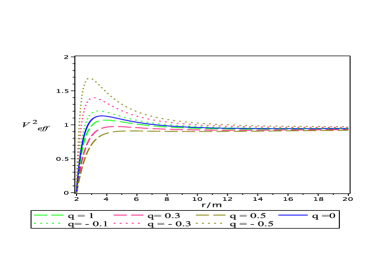
Figure 2: The effective potential for timelike geodesics on the equatorial plane as a function of the radius for different values of the quadrupole parameter. Here we set $l^{2}=20$ for concreteness.

IV.1 Circular orbits

We will now investigate the properties of circular orbits on the equatorial plane, $\theta=\pi/2$ of the gravitational described by the approximate metric (1). Circular orbits correspond to the limiting case $\dot{r}=0$. Their stability properties are determined by the extrema of the effective potential. Following the conventional stability analysis of circular orbits involving a potential function, from Eq.(38), we obtain

$$V_{eff,r}= \frac{2\epsilon m}{r^{2}}+\frac{2\left(3m-r\right)l^{2}}{r^{4}}+\frac{qm}{r^{2}\left(r-m\right)^{2}}$$ (41)

$$\times \bigg{[}\left(2m^{2}-4mr+r^{2}\right)\epsilon$$

$$+ \frac{2\left(6m^{2}-10mr+3r^{2}\right)l^{2}}{r^{2}}\bigg{]}\ ,$$

and

$$V_{eff,rr}=B_{1}+B_{2}$$ (42)

where $B_{1}$ and $B_{2}$ are given by

$$B_{1}=\frac{m\left(36m^{4}-90m^{3}r+74m^{2}r^{2}-22mr^{3}+2r^{4}\right)}{r^{3}\left(3m^{2}-4mr+r^{2}\right)^{2}}\ ,$$ (43)

$$B_{2}=\frac{mq\left(36m^{4}-114m^{3}r+74m^{2}r^{2}-17mr^{3}+r^{4}\right)}{r^{3}\left(3m^{2}-4mr+r^{2}\right)^{2}}$$ (44)

where we set $\epsilon=1$ and replaced the value of the angular momentum

$$l^{2} =\frac{\epsilon mr^{2}}{\left(r-m\right)\left(r-3m\right)^{2}}\bigg{[}2\left(3m^{2}-4mr+r^{2}\right)$$ (45)

$$+ q\left(r^{2}-6m^{2}\right)\bigg{]},$$

which can be derived from the condition $V_{eff,r}=0$.

The numerical analysis of the stability condition, $V_{eff,rr}>0$, is depicted in Fig.3.

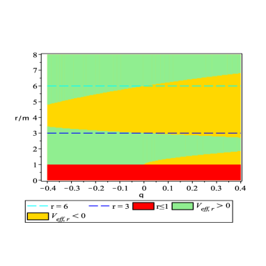
Figure 3: Stability analysis of circular orbits with radius $r/m$ for different values of the quadrupole parameter $q$. Green (yellow) points represent stable (unstable) orbits. The red region lies inside the singularity.

The green region contains only stable orbits whereas the yellow region corresponds to unstable orbits. For comparison, we include the limiting values of the Schwarzschild spacetime. We see that the quadrupole parameter $q$ changes the value of the minimum allowed radius ($3m$) and of the inner most stable circular orbit radius ($6m$) of the Schwarzschild metric. In fact, the quadrupole leads to the appearance of a second stable region below and over the radius $3m$, which is not present in the Schwarzschild limiting case. This region can reach the value of $r/m\approx 1$, approaching the singularity which is located at $r=m$. Moreover, within the spacetime determined by the interval $r\in(m,2m]$, we notice that most of this region allows the existence of stable circular orbits with a disjoint region of instability for positive values of $q$.

Furthermore, the energy of test particles on circular orbits can be expressed as

$${E}^{2}=\frac{\epsilon\left(r-2m\right)^{2}}{r\left(r-3m\right)}\bigg{[}1-\frac{mq\left(r-6m\right)}{2\left(r-m\right)\left(r-3m\right)}\bigg{]}.$$ (46)

In Fig. 4, we plot the regions in which the energy $E^{2}$ and angular momentum $l^{2}$ are both positive or negative simultaneously. The red region denotes all the radii that are not allowed for circular orbits because either the squared of the energy or of the angular momentum are negative. A comparison with Fig. 3 shows that the region contained between the singularity $r/m=1$ and around $r/m=3$ is allowed for circular orbits by the stability condition but is excluded by the energy and angular momentum conditions.

We conclude that the effect of the quadrupole on the properties of circular orbits is as follows. A positive quadrupole leads to an increase of the minimum allowed radius whereas a negative quadrupole generates the opposite effect. This means that only in the case of an oblate object, test particles are allowed to exist on orbits closer to the singularity, which is situated at $r=m$.

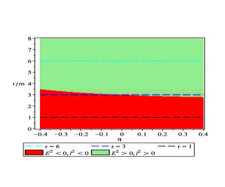
Figure 4: Energy $E^{2}$ and angular momentum $l^{2}$ of test particles on circular orbits in terms of the radius $r/m$ and the quadrupole parameter $q$.

Finally, we consider the angular velocity

$$\Omega(r)= \dot{\varphi}=\frac{1}{r}\bigg{[}\frac{m}{r-3m}\bigg{]}^{1/2}$$ (47)

$$\times\bigg{[}1+\frac{q\left(6m^{2}-4mr+r^{2}\right)}{4\left(r-m\right)\left(r-3m\right)}\bigg{]},$$

and the period

$$T(r) = \int\frac{\dot{t}}{\dot{\varphi}}d\varphi=2\pi\frac{dt}{d\varphi}$$ (48)

$$= 2\pi r^{3/2}m^{-\frac{1}{2}}\bigg{[}1-\frac{q\left(r-4m\right)}{4\left(r-m\right)}\bigg{]},$$

of circular orbits. The behavior of the angular velocity and period are depicted in Fig. (5). We can see that the influence of the quadrupole on the value of the angular velocity increases as the radius of the orbit approaches the value of $r\approx 3m$. This agrees with the behavior of the stability condition and the energy and angular momentum shown in Figs. 3 and 4, respectively. For a given orbit radius, the angular velocity increases (decreases) for positive (negative) values of the quadrupole. Notice that close to the singularity located at $r=m$, there is a region in which the angular velocity is a well behaved function of $q$ and $r$. This region corresponds to the stability region that was also found in Fig. 3.

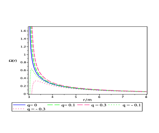
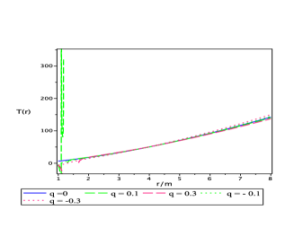
Figure 5: Angular velocity and period of circular orbits in terms of the radius $r/m$ and the quadrupole parameter $q$.

IV.2 Bounded and unbounded orbits

We now study the influence of the quadrupole on the trajectories of massive test particles, moving along unbounded paths on the equatorial plane. The geodesics for different values of the quadrupole parameter are given in Figs. 6-7, where the radial coordinate is dimensionless ($r/m$).

We consider first unbounded Schwarzschild trajectories with non-zero initial radial velocities under the influence of the quadrupole. In this case, we see that for the chosen initial angular and radial velocities all the particles escape from the gravitational field of central slightly deformed body. This is illustrated Fig.6. The direction along which the particle escapes to infinity depends on the value of the quadrupole. It is worth noticing that, in principle, this effect could be used to measure the quadrupole of the central mass distribution.

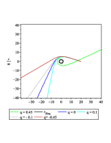
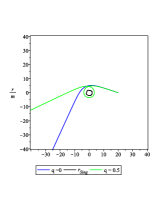
Figure 6: Influence of the quadrupole on unbounded orbits. Initial conditions: $\varphi(0)=\pi/2,\ r(0)=7,\ \dot{\varphi}(0)=0.07145$, $\dot{r}(0)=0$ (top, left); $\varphi(0)=0,\ r(0)=20,\ \dot{\varphi}(0)=0.04305$, $\dot{r}(0)=-2.5$ (top, right); $\varphi(0)=0$, $r(0)=20$, $\dot{\varphi}(0)=0.04305$, $\dot{r}(0)=-2.489$ (bottom) ;

In Fig. 7, we consider a Schwarzschild bounded orbit with zero initial radial velocity and the same non-zero value for the initial angular velocity. The left panel shows the Schwarzschild geodesic. The central and right panels illustrate the influence of a negative and positive small quadrupole, respectively. We conclude that that the small quadrupole does not affect the bounded character of the geodesic, but it does drastically modify the morphology of the trajectories.

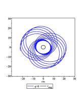
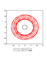
Figure 7: Influence of the quadrupole on Schwarzschild bounded orbits with vanishing initial radial velocity ($\dot{r}(0)=0)$. The initial conditions are $\varphi(0)=0$, $r(0)=7$, and $\dot{\varphi}(0)=0.08$ for all the trajectories.

We conclude that the quadrupole always affects the Schwarzschild trajectories. The explicit modifications depend on the properties of the original Schwarzschild trajectory and the value of the quadrupole parameter.

IV.3 Radial geodesics and repulsive gravity

We now study the free fall of test particles. To this end, we consider the geodesics equations in their most general form as given in Eqs.(32)-(35). The important point is that in all the cases to be considered all the initial spatial velocities are assumed to vanish. The starting point can be chosen arbitrarily, but some special values of the angle $\theta$ are of interest, namely, the symmetry axis $\theta=0$, the equatorial plane $\theta=\pi/2$, and some other different value that we can choose as $\theta=\pi/4$. In fact, in Boshkayev2016 , it was shown that by analyzing the behavior of radial geodesics one can detect the presence of repulsive gravity defelice89 ; lq12 ; lq14

A free falling particle will continue its motion along the radial direction, unless a force acts on it and changes the original radial direction. This phenomenon has been reported in the case of an exact solution with quadrupole moment in Boshkayev2016 .

We will now consider the same situation in the case of the approximate solution we are analyzing in this work. The result of the integration of the geodesic equations (32)-(35) is illustrated in Fig. 8. We see that, in fact, free falling particles move along the original directions ($\theta=0$, $\theta=\pi/4$, and $\theta=\pi/2$), independently of the value of quadrupole parameter $q$. This means that no repulsive gravity effects can be detected in the case of the approximate metric. Taking into account also the result of Boshkayev2016 , we conclude that repulsive effects are non-linear, i.e., they appear only in the case of an exact quadrupolar metric.

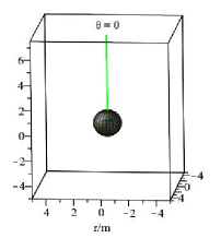
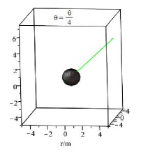
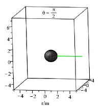
Figure 8: Free fall of test particles with vanishing initial velocities. On the axes $\theta=0$ (top, left), $\theta=\pi/4$ (top, right), and $\theta=\pi/2$ (bottom). The sphere represents the singularity at the radius $r=m$ (top). The trajectories of the free falling test particles do not depend on the value of the parameter $q$. For concreteness, we set the energy of the test particle as $E=1$.

V Conclusions and remarks

In this work, we have derived a family of approximate vacuum solutions of Einstein equations with quadrupole. Among all the solutions contained in this family we choose a particular one, which presents a naked singularity at the hypersurface $r=m$, instead of $r=2m$ as in other quadrupolar metrics. To our knowledge this is the only metric with such a singularity.

By applying an appropriate coordinate transformation, we found the Newtonian limit of the approximate solution and showed that it corresponds to the gravitational potential of a mass with quadrupole.

Then, we investigated the motion of test particles along circular orbits. We established that a positive quadrupole leads to an increase of the minimum allowed radius whereas a negative quadrupole generates the opposite effect. This means that only in the case of an oblate object, test particles are allowed to exist on orbits closer to the singularity, which is situated at $r=m$. In the case of bounded and unbounded trajectories, we found that the quadrupole always affects the Schwarzschild trajectories. The explicit modifications depend on the properties of the original Schwarzschild trajectory and the value of the quadrupole parameter.

Finally, we analyzed radial geodesics that have been used previously to detect effects of repulsive gravity in an exact quadrupolar metric. However, in the case of the approximate solution no repulsive effects were found. We conclude that repulsive gravity in the the quadrupolar naked singularities is a non-linear phenomenon.

References

- (1) R.P. Kerr, Physical review letters 11(5), 237 (1963)
- (2) K.S. Thorne, C.W. Misner, J.A. Wheeler, Gravitation (Freeman, 2000)
- (3) H. Quevedo, Mass Quadrupole as a Source of Naked Singularities. Int. J. Mod. Phys. D 20, 1779–1787 (2011)
- (4) M. Heusler, Black hole uniqueness theorems (Cambridge University Press, 1996)
- (5) M. Abishev, K. Boshkayev, H. Quevedo, S. Toktarbay, in Accretion disks around a mass with quadrupole. Gravitation, Astrophysics, and Cosmology, 185-186 (2016)
- (6) K. Boshkayev, E. Gasperín, A.C. Gutiérrez- Piñeres, H. Quevedo, S. Toktarbay, Motion of test particles in the field of a naked singularity. Phys. Rev. D 93, 024024 (2016)
- (7) K. Boshkayev, H. Quevedo, S. Toktarbay, B. Zhami, M. Abishev, Grav. Cosmol. 22(4), 305 (2016)
- (8) D.M. Zipoy, Journal of Mathematical Physics 7(6), 1137 (1966)
- (9) B. Voorhees, Physical Review D 2(10), 2119 (1970)
- (10) D. Malafarina, G. Magli, L. Herrera, in AIP Conference Proceedings, vol. 751 (American Institute of Physics, 2005), vol. 751, pp. 185–187
- (11) H. Stephani, D. Kramer, M. MacCallum, C. Hoenselaers, E. Herlt, Exact solutions of Einstein’s field equations (Cambridge University Press, 2003)
- (12) F. Frutos-Alfaro, H. Quevedo, P.A. Sanchez, Royal Society open science 5(5), 170826 (2018)
- (13) M. Abishev, N. Beissen, F. Belissarova, K. Boshkayev, A. Mansurova, A. Muratkhan, H. Quevedo, S. Toktarbay, International Journal of Modern Physics D 30(13), 2150096 (2021)
- (14) A. Allahyari, H. Firouzjahi, B. Mashhoon, Quasinormal modes of a black hole with quadrupole moment. Phys. Rev. D 99, 044005 (2018)
- (15) D. Pugliese, H. Quevedo, R. Ruffini, Phys. Rev. D 83, 024021 (2011)
- (16) D. Pugliese, H. Quevedo, R. Ruffini, Physical Review D 83(2), 024021 (2011)
- (17) F. De Felice, in Annales de Physique Colloque Supplement, vol. 14 (1989), vol. 14, pp. 79–83
- (18) O. Luongo, H. Quevedo, in The Twelfth Marcel Grossmann Meeting: On Recent Developments in Theoretical and Experimental General Relativity, Astrophysics and Relativistic Field Theories (In 3 Volumes) (World Scientific, 2012), pp. 1029–1031
- (19) O. Luongo, H. Quevedo, Physical Review D 90(8), 084032 (2014)