Scaling limit of the collision measures of multiple random walks

Abstract

For an integer $k\geq 2$, let $S^{(1)},S^{(2)},\dots,S^{(k)}$ be $k$ independent simple symmetric random walks on $\mathbb{Z}$. A pair $(n,z)$ is called a collision event if there are at least two distinct random walks, namely, $S^{(i)},S^{(j)}$ satisfying $S^{(i)}_{n}=S^{(j)}_{n}=z$. We show that under the same scaling as in Donsker’s theorem, the sequence of random measures representing these collision events converges to a non-trivial random measure on $[0,1]\times\mathbb{R}$. Moreover, the limit random measure can be characterized using Wiener chaos. The proof is inspired by methods from statistical mechanics, especially, by a partition function that has been developed for the study of directed polymers in random environments.

1 Introduction

For an integer $k\geq 2$, let $S^{(1)},S^{(2)},\dots,S^{(k)}$ be $k$ independent simple symmetric random walks (SSRWs) on $\mathbb{Z}$, defined on a probability space $(\Omega,\mathcal{A},\mathbf{P})$ (see [20, p.3]). A pair $(n,z)\in\mathbb{N}\times\mathbb{Z}$ is called a collision event if there are at least two random walks that collide (occupy the same position at the same time) at the time $n$ and the location $z$ (see Figure 1), and $n$ is then called a collision time.
First mentioned in Pólya’s note [18], the collision of random walks has since then been a classic topic in probability theory. Recently, this topic has gained more attention from researchers working on the random walks on graphs [4, 12] and random environments [11, 9, 3].
When consider only two random walks, collision problems are strongly related to Brownian local time [15, 19, 23]. The convergence of collision times can be achieved by coupling a new SSRW, the difference between two given random walks, with a Brownian motion using Skorokhod’s embedding [20, p.52][10, Theorem 8.6.1]. However, these methods cannot be easily adapted to give convergence results for the collisions of more than two SSRWs because the couplings rely heavily the choices of stopping times which are proper for each SSRW.
To the best of our knowledge, scaling limit results for collisions of $k>2$ random walks are still limited.
In this paper, we investigate a relatively uncommon aspect of random walk collisions, concerning their duality with the partition function of a directed polymer model in statistical mechanics [8]. By following the ideas developped in [8, 2], we obtain new results on when and where the collisions of these random walks occur after long observation, or more precisely, on the scaling limit of the empirical measures of the collision events.

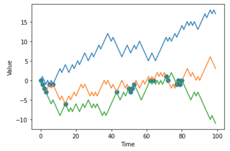
Figure 1: An example of collision events when $k=3,N=100$. The collision events are represented by blue dots.

Our study objects are as follows:

Definition 1.1.

For each $N\in\mathbb{N}$, we define the collision measures of $k$ random walks $S^{(1)},S^{(2)},\dots,S^{(k)}$ until time $N$ to be:

$$\Pi_{N}:=\sum_{n=1}^{N}\sum_{z\in\mathbb{Z}}\sum_{\begin{subarray}{c}1\leq i<j\leq k:\\ S_{n}^{(i)}=S_{n}^{(j)}=z\end{subarray}}\delta_{\left(\frac{n}{N},\frac{z}{\sqrt{N}}\right)},\text{ and}$$

$$\Pi^{\prime}_{N}:=\sum_{n=1}^{N}\sum_{z\in\mathbb{Z}}\delta_{\left(\frac{n}{N},\frac{z}{\sqrt{N}}\right)}\mathbb{1}_{\{(n,z)\text{ is an collision event}\}},$$

where $\delta$ is the Dirac measure.

For each $N\in\mathbb{N}$, the main difference between $\Pi^{\prime}_{N}$ and $\Pi_{N}$ is that $\Pi_{N}$ takes into account the multiplicity of collision events. For example, if the number of considered random walks is $3$ and it happens that $S^{(1)}_{n}=S^{(2)}_{n}=S^{(3)}_{n}=z$ for some $(n,z)$, then the Dirac measure $\delta_{(\frac{n}{N},\frac{z}{\sqrt{N}})}$ will appear $3$ times in the summation in $\Pi_{N}$ while the number of its appearance in $\Pi^{\prime}_{N}$ is still one.
Concerning the scaling choice, one can observe that this is the same scaling as in Donker’s theorem, which also suggests that the distribution of $\hat{\Pi}_{N}$ is closely related to Brownian local time. Indeed, when $k=2$, the total measure of $\Pi_{N}$ is equal to

$$\#\{n\in[\![1,N]\!]:S^{(1)}_{n}-S^{(2)}_{n}=0\}\stackrel{{\scriptstyle(d)}}{{=}}\#\{n\in[\![1,N]\!]:S^{(1)}_{2n}=0\}=L^{0}_{S^{(1)}}\left(2N\right),$$ (1)

where $\stackrel{{\scriptstyle(d)}}{{=}}$ is the equality in law, and $L^{0}_{S}(t)$ is the local time at position $0$ during the period $[0,t]$ of some walk $S$. So by the convergence of local time of simple random walks, the equation (1) implies $\frac{1}{\sqrt{N}}\left\|\Pi_{N}\right\|=O_{\mathbf{P}}(1)$, where $\|\Pi_{N}\|$ denotes the total measure of $\Pi_{N}$.
In this work, we not only bound the sequence $(\frac{1}{\sqrt{N}}\Pi_{N};N\in\mathbb{N})$, but also prove that this sequence of random measures converges to a non-trivial random measure $\mathcal{N}$ on $[0,1]\times\mathbb{R}$. Before giving our main result, let us recall the convergence of random measures.

Definition 1.2.

(Convergence of random measures) Suppose $\xi,\xi_{1},\xi_{2},\dots$ are random finite measures on $([0,1]\times\mathbb{R},\mathcal{B}([0,1]\times\mathbb{R}))$, we say that $\xi_{n}\xrightarrow[n\rightarrow\infty]{wd}\xi$ if the sequence of real random variables $(\xi_{n}(f),n\in\mathbb{N})$ converges in distribution to $\xi(f)$ when $n$ goes to infinity for all bounded continuous function $f\in\mathcal{C}_{b}([0,1]\times\mathbb{R})$. Here, $\mu(f)$ denotes the integral $\int fd\mu$ for any (random) measure $\mu$ and bounded measurable function $f$.

Here are our main results:

Theorem 1.3.

(Convergence of collision measures and characterization of the limit random measure)

• There is a random finite positive measure $\mathcal{N}$ on the measurable space $([0,1]\times\mathbb{R},\mathcal{B}([0,1]\times\mathbb{R}))$ such that:

  $$\frac{1}{\sqrt{N}}\Pi_{N}\xrightarrow[N\rightarrow+\infty]{wd}\mathcal{N}\qquad\text{ and }\qquad\frac{1}{\sqrt{N}}\Pi^{\prime}_{N}\xrightarrow[N\rightarrow+\infty]{wd}\mathcal{N}.$$

• Furthermore, for all nonnegative bounded continuous function $f\in\mathcal{C}_{b,+}([0,1]\times\mathbb{R})$, the exponential moment of $\mathcal{N}$ with respect to $f$ is equal to $k$-th moment of a positive random variable $\mathcal{Z}_{\sqrt{2f}}$:

  $$\mathbf{E}\left[e^{\mathcal{N}(f)}\right]=\mathbf{E}\left[\left(\mathcal{Z}_{\sqrt{2f}}\right)^{k}\right].$$

  where for each $a\in\mathcal{C}_{b,+}([0,1]\times\mathbb{R})$, the random variable $\mathcal{Z}_{a}$ is identified as the sum of multiple stochastic integrals given by:

  $$\mathcal{Z}_{a}:=1+\sum_{n=1}^{\infty}\int_{\Delta_{n}}\int_{\mathbb{R}^{n}}\prod_{i=1}^{n}\bigg{[}a(\mathbf{t}_{i},\mathbf{x}_{i})\varrho(\mathbf{t}_{i}-\mathbf{t}_{i-1},\mathbf{x}_{i}-\mathbf{x}_{i-1})W(d\mathbf{t}_{i}d\mathbf{x}_{i})\bigg{]},$$ (2)

  where, $W$ is the white noise based on the Lebesque measure on $[0,1]\times\mathbb{R}$, $\mathbf{x}_{0}=0$, $\varrho$ is the standard Gaussian heat kernel

  $$\varrho(t,x)=\frac{e^{-x^{2}/2t}}{\sqrt{2\pi t}},$$

  and $\Delta_{n}$ is the $n$-dimensional simplex

  $$\Delta_{n}:=\{\mathbf{t}\in[0,1]^{n}:0=\mathbf{t}_{0}<\mathbf{t}_{1}<\mathbf{t}_{2}<\cdots<\mathbf{t}_{n}\leq 1\}.$$ (3)

We refer to [25, Chapter 1] for an introduction on white noise (see also Section 3.2 of this article).
As mentioned earlier, we will prove this theorem by investigating the connection between the collision measures of random walks with a model in statistical mechanics; hence, we will introduce many auxiliary notions in our paper, such as random environment $\omega$, partition function $\mathfrak{Z}_{N}$ and $U$-statistics $\mathcal{S}^{N}_{n}(\cdot)$.
The general idea is that by associating each point $(n,z)$ on the grid $\mathbb{N}\times\mathbb{Z}$ with a random variable, we can change the underlying framework from studying a deterministic grid to studying a collection of random variables indexed by $\mathbb{N}\times\mathbb{Z}$. For a such collection, the range of possible tools from statistical mechanics is large. Indeed, the partition function we will use is developped to study a directed polymer model [2, 5].
The organization of this paper is as follows: Section 2 introduces some basic notions that we will use in the sequel to explain our main ideas, especially, the relation between the concept of partition functions and the collision measures $\Pi_{N}$. Section 3 gives a brief review on $U$-statistics and Wiener chaos. At the end of this section, we prove some new theorems on the convergence of $U$-statistics, on which our asymptotic result on partition functions (Theorem 2.3) is based. Section 4 presents a short study on the random variable $\mathcal{Z}_{a}$ defined in (2), and our proof of Theorem 2.3. Finally, Section 5 combines all proved results to show the weak tightness of $(\frac{1}{\sqrt{N}}\Pi_{N},N\in\mathbb{N})$, and prove Theorem 1.3.
Some auxiliary results are presented in the Appendix at the end of this article.

2 Partition functions and main ideas of proof

2.1 Partition functions

We introduce a collection $\omega:=\left(\omega(i,z):i\in\mathbb{N},z\in\mathbb{Z}\right)$ of independent Rademacher variables indexed by $\mathbb{N}\times\mathbb{Z}$, i.e., for all $(n,z)\in\mathbb{N}\times\mathbb{Z}$,

$$\mathbf{P}(\omega(n,z)=-1)=\mathbf{P}(\omega(n,z)=1)=\frac{1}{2}.$$

These random variables are created by extending our existing probability space $(\Omega,\mathcal{A},\mathbf{P})$ so that $\omega,S^{(1)},S^{(2)},\dots,S^{(k)}$ are independent.
In the sequel, for a real number $\beta$ and a real function $A$ on $\mathbb{N}\times\mathbb{Z}$, $\beta\omega$ and $A\omega$ are defined as:

$$A\omega :=\left(A(i,z)\omega(i,z):i\in\mathbb{N},z\in\mathbb{Z}\right).$$

$$\beta\omega :=\left(\beta\omega(i,z):i\in\mathbb{N},z\in\mathbb{Z}\right).$$

As briefly explained in Section 1, the role $\omega$ is to add new degrees of freedom to the existing model, by which we have more flexibility to create more objects. The partition function $\mathfrak{Z}$ is one of such objects:

Definition 2.1.

For any positive integer $N$ and any real function $A$ on $\mathbb{N}\times\mathbb{Z}$, the partition function $\mathfrak{Z}_{N}(A)$ is defined as the conditional expectation:

$$\mathfrak{Z}_{N}(A):=\mathbf{E}\left[\text{ }\prod_{n=1}^{N}(1+A(n,S^{(1)}_{n})\omega(n,S^{(1)}_{n}))\text{ }\bigg{|}\text{ }\omega\text{ }\right].$$

Note that $\mathfrak{Z}_{N}(A)$ is a random variable depending only on the value of $\omega$.

2.2 Main ideas

The starting point of our paper and the proof of our main results is a heuristic relation between the partition functions $\mathfrak{Z}_{N}$ and the random measure $\Pi_{N}$:
Given a nonnegative bounded function $A$ on $\mathbb{N}\times\mathbb{Z}$, since $S^{(1)},\cdots,S^{(k)}$ are i.i.d., we have:

$$\mathbf{E}\left[\mathfrak{Z}_{N}\left(\frac{1}{N^{1/4}}A\right)^{k}\right]=\mathbf{E}\left[\mathbf{E}\left[\prod_{n=1}^{N}(1+\frac{1}{N^{1/4}}A(n,S^{(1)}_{n})\omega(n,S^{(1)}_{n}))\bigg{|}\omega\right]^{k}\right]$$

$$= \mathbf{E}\Bigg{[}\mathbf{E}\left[\prod_{i=1}^{k}\prod_{n=1}^{N}(1+\frac{1}{N^{1/4}}A(n,S^{(i)}_{n})\omega(n,S^{(i)}_{n}))\bigg{|}\omega\right]\Bigg{]}$$

$$= \mathbf{E}\left[\prod_{n=1}^{N}\prod_{i=1}^{k}(1+\frac{1}{N^{1/4}}A(n,S^{(i)}_{n})\omega(n,S^{(i)}_{n}))\right]$$

$$= \mathbf{E}\left[\mathbf{E}\left[\prod_{n=1}^{N}\prod_{i=1}^{k}(1+\frac{1}{N^{1/4}}A(n,S^{(i)}_{n})\omega(n,S^{(i)}_{n}))\bigg{|}S^{(1)},\cdots,S^{(k)}\right]\right]$$

$$= \mathbf{E}\left[\prod_{n=1}^{N}\mathbf{E}\left[\prod_{i=1}^{k}(1+\frac{1}{N^{1/4}}A(n,S^{(i)}_{n})\omega(n,S^{(i)}_{n}))\bigg{|}S^{(1)},\cdots,S^{(k)}\right]\right]$$

$$= \mathbf{E}\bigg{[}\prod_{n=1}^{N}\bigg{[}1+\frac{1}{N^{1/2}}\bigg{(}\sum_{\begin{subarray}{c}1\leq i<j\leq k:\\ S_{n}^{(i)}=S_{n}^{(j)}=z\end{subarray}}A^{2}(n,z)\bigg{)}+\frac{1}{N^{3/4}}(\dots)+...\bigg{]}\bigg{]}$$

Then since $1+x\approx e^{x}$, heuristically, we deduce:

$$\mathbf{E} \left[\mathfrak{Z}_{N}\left(\frac{1}{N^{1/4}}A\right)^{k}\right]\approx\mathbf{E}\bigg{[}\prod_{n=1}^{N}\bigg{[}\exp\big{(}\frac{1}{N^{1/2}}\sum_{\begin{subarray}{c}1\leq i<j\leq k:\\ S_{n}^{(i)}=S_{n}^{(j)}=z\end{subarray}}A^{2}(n,z)\big{)}\bigg{]}\bigg{]}$$

$$= \mathbf{E}\bigg{[}\exp\bigg{(}\frac{1}{N^{1/2}}\sum_{n=1}^{N}\sum_{\begin{subarray}{c}1\leq i<j\leq k:\\ S_{n}^{(i)}=S_{n}^{(j)}=z\end{subarray}}A^{2}(n,z)\bigg{)}\bigg{]}=\mathbf{E}\bigg{[}\exp\bigg{(}\frac{1}{N^{1/2}}\Pi_{N}(f_{N})\bigg{)}\bigg{]},$$

where $f_{N}$ is a measurable function such that $f_{N}\left(\frac{n}{N},\frac{z}{\sqrt{N}}\right)=A(n,z)$ for all $n\in\mathbb{N},z\in\mathbb{Z}$.
In short, by abuse of notation, the above observation suggests that:

$$\mathbf{E}\left[e^{N^{-1/2}\Pi_{N}}\right]\approx\mathbf{E}\left[(\mathfrak{Z}_{N})^{k}\right].$$ (4)

In other words, if we have a good understanding of $\mathfrak{Z}$, we will have good information on $\Pi_{N},\Pi^{\prime}_{N}$.
Then to study the partition function $\mathfrak{Z}_{N}$, we base our study on the paper [2], in which Alberts et al. studied the scaling limit of $\mathfrak{Z}$ when the function $A$ is constant. In our study, we generalize their results for a sequence of functions $(A_{N},N\in\mathbb{N})$ satisfying certain conditions. An expansion of Wiener chaoses emerges naturally in our limit objects because, as we will see, each term in the algebraic expansion of $\mathfrak{Z}_{N}$ (cf. Proposition 4.6) converges to a Wiener chaos. To this aim, we will have to introduce some $U$-statistics and study their asymptotic behavior in Section 3.

2.3 Main results on partition functions

We terminate this section by presenting our results on the asymptotic behavior of $\mathfrak{Z}_{N}$. The proofs will be presented later in Section 4.

Notation 2.2.

For $(t,x)\in[0,1]\times\mathbb{R}$, $[t,x]_{N}$ denotes the unique pair of integer $(i,z)$ such that :

• $(t,x)\in\left(\frac{i-1}{N},\frac{i}{N}\right]\times\left(\frac{z-1}{\sqrt{N}},\frac{z+1}{\sqrt{N}}\right]$,

• $i$ and $z$ have same parity.

Theorem 2.3.

Let $(A_{n},n\in\mathbb{N})$ be a sequence of real functions whose domain is $\mathbb{N}\times\mathbb{Z}$ such that:

• $\sup_{N}\|A_{N}\|_{\infty}<+\infty$,

• there is a measurable function $a\in L^{\infty}([0,1]\times\mathbb{R})$ such that:

  $$\lim_{N\rightarrow+\infty}A_{N}([t,x]_{N})=a(t,x)\quad\text{a.e.}$$

Then as $N$ converges to infinity, we have:

$$\mathfrak{Z}_{N}(N^{-1/4}A_{N})\xrightarrow{\text{(d)}}\mathcal{Z}_{\sqrt{2}a}$$

This theorem is a generalization of Proposition 5.3 in [2] where the sequence $(A_{N};N\in\mathbb{N})$ is replaced by a fixed constant $\beta\geq 0$.
We will also prove that under some conditions, the partition functions are uniformly bounded in $L^{k}$:

Theorem 2.4.

For a sequence of real functions $(A_{n},n\in\mathbb{N})$ on $\mathbb{N}\times\mathbb{Z}$ such that $\sup_{N}\|A_{N}\|_{\infty}<+\infty$, we have:

$$\limsup_{N}\mathbf{E}\left[\left(\mathfrak{Z}_{N}\left(N^{-1/4}A_{N}\right)\right)^{k}\right]<+\infty.$$

Notice that even though $k$ is fixed in our study, the definition of $\mathfrak{Z}$ does not depend on $k$. So, the above sequence $\left(\mathfrak{Z}_{N}\left(N^{-1/4}A_{N}\right),N\in\mathbb{N}\right)$ is also uniformly bounded in $L^{p}$ for all $p\in\mathbb{N}$, which implies directly the following corollary:

Corollary 2.5.

For a sequence of real functions $A_{1},A_{2},...$ on $\mathbb{N}\times\mathbb{Z}$ such that $\sup_{N}\|A_{N}\|_{\infty}<+\infty$, the sequence of random variables $\left(\mathfrak{Z}_{N}\left(N^{-1/4}A_{N}\right),N\in\mathbb{N}\right)$ is uniformly $L^{k}$-integrable.

3 $U$-Statistics: related notions and limit theorems

Let $E^{N}_{n}:=\{\mathbf{i}\in[\![1,N]\!]^{n}:\mathbf{i}_{j}\neq\mathbf{i}_{l}\text{ for }j\neq l\}$. In this paper, we are interested in sums of the form:

$$\sum_{\mathbf{i}\in E^{N}_{n}}\sum_{\begin{subarray}{c}\mathbf{z}\in\mathbb{Z}^{n}\\ \mathbf{i}\leftrightarrow\mathbf{z}\end{subarray}}\overline{g_{N}}(\mathbf{i},\mathbf{z})A_{N}(\mathbf{i},\mathbf{z})\omega(\mathbf{i},\mathbf{z}),$$ (5)

for some weight functions $\overline{g_{N}}$ specified later. The notation $\mathbf{i}\leftrightarrow\mathbf{z}$ means that:

Notation 3.1.

$\mathbf{i}\leftrightarrow\mathbf{z}$ means that for all $j\in[\![1,n]\!]$, the corresponding $j$-th coordinates of $\mathbf{i}$ and $\mathbf{z}$, namely $\mathbf{i}_{j}$ and $\mathbf{z}_{j}$, have the same parity.

We will see that sums of this type appear naturally when we expand the partition functions $\mathfrak{Z}_{N}$ (see (19)).
The organization of this section is as follows: Sections 3.1 and 3.2 introduce the framework of Theorem 3.12 which is our main result on the convergence of sums of the form (5). Section 3.3 presents the proof of Theorem 3.12 and other related results.
The approach we used in this section is standard in the theory of $U$-statistics. Interested readers can consult the book [16] of Korolyuk and Borovskikh for a more rigourous introduction of this theory.

3.1 Introduction of $U$-statistics $S^{N}_{n}$

We first make precise the definition of the weight functions $(\overline{g_{N}},N\in\mathbb{N})$ in the above sum.
Let $g$ be a function in $L^{2}([0,1]^{n}\times\mathbb{R}^{n})$. For each $N$, the weight functions $\overline{g_{N}}$ associated to $g$ is defined by the following procedure:
First, we partition the space $(0,1]^{n}\times\mathbb{R}^{n}$ in rectangles of the form:

$$\mathcal{R}^{N}_{n}:=\left\{\left(\frac{\mathbf{i}-\mathbf{1}}{N},\frac{\mathbf{i}}{N}\right]\times\left(\frac{\mathbf{z}-1}{\sqrt{N}},\frac{\mathbf{z}+\mathbf{1}}{\sqrt{N}}\right]:\mathbf{i}\in D^{N}_{n},\mathbf{z}\in\mathbb{Z}^{n},\mathbf{i}\leftrightarrow\mathbf{z}\right\}.$$

with $\mathbf{1}$ being the vector of ones and $D^{N}_{n}$ being the integer simplex:

$$D^{N}_{n}:=\{\mathbf{i}\in[\![1,N]\!]^{n}:1\leq\mathbf{i}_{1}<\mathbf{i}_{2}\dots<\mathbf{i}_{n}\leq N\}.$$ (6)

Visually, $\mathcal{R}^{N}_{n}$ is a collection of nonoverlapping translations of the base rectangle:

$$\left(\frac{0}{N},\frac{1}{N}\right]^{n}\times\left(\frac{-1}{\sqrt{N}},\frac{1}{\sqrt{N}}\right]^{n}.$$

Then, the function $\overline{g_{N}}$ is defined as the average of $g$ on each rectangles above.
More precisely, for any $(\mathbf{t},\mathbf{x})\in(0,1]^{n}\times\mathbb{R}^{n}$, $\overline{g_{N}}(\mathbf{t},\mathbf{x})$ is defined as the mean:

$$\overline{g_{N}}(\mathbf{t},\mathbf{x}):=\frac{1}{|R|}\int_{R}g(\mathbf{s},\mathbf{y})d\mathbf{s}\,d\mathbf{y},$$

where $R$ is the unique rectangle in $\mathcal{R}^{N}_{n}$ that contains $(\mathbf{t},\mathbf{x})$, and $|R|$ denotes the Lebesque measure of $R$. In probabilistic terms, $\overline{g_{N}}$ is simply the conditional expectation of $g$ onto the rectangles of $\mathcal{R}^{N}_{n}$. We note that $|R|=2^{n}N^{-3n/2}$. This term will appear recurrently in most of our computations.
Suppose $(A_{N},N\in\mathbb{N})$ is a sequence of real-valued functions on $\mathbb{N}\times\mathbb{Z}$.

Notation 3.2.

For any $n$-tuple $\mathbf{i}\in E^{N}_{n}$ and $n$-tuple $\mathbf{z}\in\mathbb{Z}^{n}$, $A_{N}(\mathbf{i},\mathbf{z})$ and $\omega(\mathbf{i},\mathbf{z})$ denote

$$A_{N}(\mathbf{i},\mathbf{z}) :=A_{N}(\mathbf{i}_{1},\mathbf{z}_{1})A_{N}(\mathbf{i}_{2},\mathbf{z}_{2})...A_{N}(\mathbf{i}_{n},\mathbf{z}_{n}),$$

$$\omega(\mathbf{i},\mathbf{z}) :=\omega(\mathbf{i}_{1},\mathbf{z}_{1})\omega(\mathbf{i}_{2},\mathbf{z}_{2})...\omega(\mathbf{i}_{n},\mathbf{z}_{n}),$$

with $\mathbf{i}_{j}$ being the $j$-th coordinate of $\mathbf{i}$ as defined previously.

Now, we define the weighted $U$-statistics $\mathcal{S}^{N}_{n}$.

Definition 3.3.

Suppose $(A_{n},n\in\mathbb{N})$ is a sequence of bounded real-valued functions on $\mathbb{N}\times\mathbb{Z}$. For any function $g\in L^{2}([0,1]^{n}\times\mathbb{R}^{n})$, the $U$- statistics $\mathcal{S}^{N}_{n}$ is defined as:

$$\mathcal{S}^{N}_{n}(g):=2^{n/2}\sum_{\mathbf{i}\in E^{N}_{n}}\sum_{\begin{subarray}{c}\mathbf{z}\in\mathbb{Z}^{n}:\\ \mathbf{i}\leftrightarrow\mathbf{z}\end{subarray}}\overline{g_{N}}\left(\frac{\mathbf{i}}{N},\frac{\mathbf{z}}{\sqrt{N}}\right)A_{N}(\mathbf{i},\mathbf{z})\omega(\mathbf{i},\mathbf{z}).$$ (7)

We first give some basic properties of the $U$-statistics $S^{N}_{n}$.

Proposition 3.4.

Suppose $(A_{N},N\in\mathbb{N})$ is a sequence of bounded real-valued functions on $\mathbb{N}\times\mathbb{Z}$. For all positive integers $n$ and $N$, we have:

• (Well-posedness) $\mathcal{S}^{N}_{n}(g)$ is well-defined and has zero mean for all $g\in L^{2}([0,1]^{n}\times\mathbb{R}^{n})$.

• (Linearity) For all $f,g\in L^{2}([0,1]^{n}\times\mathbb{R}^{n})$, $\alpha,\beta\in\mathbb{R}$

  $$\mathcal{S}^{N}_{n}(\alpha f+\beta g)=\alpha\mathcal{S}^{N}_{n}(f)+\beta\mathcal{S}^{N}_{n}(g).$$

• ($L^{2}$-boundedness) If $c>0$ is a number such that such that $\|A_{N}\|_{\infty}\leq c$, then for all $g\in L^{2}([0,1]^{n}\times\mathbb{R}^{n})$ :

  $$\mathbf{E}[\mathcal{S}^{N}_{n}(g)^{2}]\leq c^{2n}N^{3n/2}\|g\|^{2}_{2}.$$

• (Uncorrelatedness of $U$-statistics of different orders) If $n_{1},n_{2}$ are two different positive integers, then $\forall g_{i}\in L^{2}([0,1]^{n_{i}}\times\mathbb{R}^{n_{i}})\quad i=1,2,$

  $$\mathbf{E}[\mathcal{S}_{n_{1}}^{N}(g_{1})\mathcal{S}_{n_{2}}^{N}(g_{2})]=0.$$

Proof.

Assume that $f$ and $g$ have compact supports, then the sums in $S^{N}_{n}(f)$ and $S^{N}_{n}(g)$ have a finite number of terms; thus, point $i$ is trivial. Point $ii$ is also trivial by recalling that $\omega$ is a collection of centered random variables. Now, for point $iii$, observe that for any $\mathbf{i},\mathbf{i}^{\prime}\in E^{N}_{n},\mathbf{x},\mathbf{x}^{\prime}\in\mathbb{Z}^{n}$:

$$\mathbf{E}\bigg{[}\prod_{l=1}^{n}\omega(\mathbf{i}_{l},\mathbf{x}_{l})\prod_{l=1}^{n}\omega(\mathbf{i}^{\prime}_{l},\mathbf{x}^{\prime}_{l})\bigg{]}=\mathbb{1}_{\{\mathbf{i}=\mathbf{i}^{\prime},\mathbf{x}=\mathbf{x}^{\prime}\}}.$$

Hence

$$\mathbf{E}\bigg{[}\mathcal{S}^{N}_{n}(g)^{2}\bigg{]} =2^{n}\sum_{\mathbf{i}\in E^{N}_{n}}\sum_{\begin{subarray}{c}\mathbf{z}\in\mathbb{Z}^{n}\\ \mathbf{i}\leftrightarrow\mathbf{z}\end{subarray}}A_{N}(\mathbf{i},\mathbf{z})^{2}\overline{g_{N}}\left(\frac{\mathbf{i}}{N},\frac{\mathbf{z}}{\sqrt{N}}\right)^{2}$$

$$\leq 2^{n}\sum_{\mathbf{i}\in[\![1,N]\!]^{n}}\sum_{\begin{subarray}{c}\mathbf{z}\in\mathbb{Z}^{n}\\ \mathbf{i}\leftrightarrow\mathbf{z}\end{subarray}}c^{2n}\frac{1}{|\mathcal{R}|}\int_{\mathcal{R}}g(\mathbf{t},\mathbf{y})^{2}d\mathbf{t}d\mathbf{y}$$

$$=N^{3n/2}c^{2n}\int_{[0,1]^{n}}\int_{\mathbb{R}^{n}}g(\mathbf{t},\mathbf{y})^{2}d\mathbf{t}\mathbf{y}.$$

The last inequality is simply an application of the Cauchy-Schwarz lemma.
So our theorem is valid for compactly supported functions. In other words, $g\mapsto S^{N}_{n}(g)$ is a linear Lipschitz continuous mapping that maps the space $L^{2}_{\text{compact}}([0,1]^{n}\times\mathbb{R}^{n})$ into $L^{2}(\mathbf{P})$. Hence, all the properties $i,ii,iii$ can be extended naturally to all $L^{2}([0,1]^{n}\times\mathbb{R}^{n})$ by the density of $L^{2}_{\text{compact}}([0,1]^{n}\times\mathbb{R}^{n})$ in $L^{2}([0,1]^{n}\times\mathbb{R}^{n})$.
For the covariance relation in point $iv$, one can observe that if $\mathbf{i}\in E^{N}_{n_{1}},\mathbf{x}\in\mathbb{Z}^{n_{1}},\mathbf{i}^{\prime}\in E^{N}_{n_{2}},\mathbf{x}^{\prime}\in\mathbb{Z}^{n_{2}}$, then

$$\mathbf{E}\bigg{[}\prod_{l=1}^{n_{1}}\omega(\mathbf{i}_{l},\mathbf{x}_{l})\prod_{l=1}^{n_{2}}\omega(\mathbf{i}^{\prime}_{l},\mathbf{x}^{\prime}_{l})\bigg{]}=0.$$

because there is necessarily one $\omega$ term that is distinct from the others, and its independence from the rest implies zero expectation.
Hence, $iv$ is clearly true if $g_{1},g_{2}$ have compact supports. The extension to non-compactly-supported functions can also be obtained by a density argument as above. ∎

Now, to characterize rigorously the limit of the $U$-statistics $(S^{N}_{n},N\geq 1)$, we need to introduce the Wiener chaos.

3.2 Wiener chaos

3.2.1 White noise and stochastic integration on $[0,1]\times\mathbb{R}$

This section recalls the elementary theory of white noise and stochastic integration on the measure space $([0,1]\times\mathbb{R},\mathcal{B},dt\otimes dx)$. Here $\mathcal{B}$ is the Borel $\sigma$-algebra, and $dt\otimes dx$ denotes Lebesque measure on $[0,1]\times\mathbb{R}$. For more details on Wiener chaos, we invite readers to read [17, Chapter 1] or [13, Chapter 11].
Let $\mathcal{B}_{f}$ be the collection of all Borel sets of $[0,1]\times\mathbb{R}$ with finite Lebesgue measure. Observe that $\mathcal{B}=\sigma(\mathcal{B}_{f})$.

Definition 3.5.

A white noise on $[0,1]\times\mathbb{R}$ is a collection of mean zero Gaussian random variables indexed by $\mathcal{B}_{f}$

$$W=\{W(A):A\in\mathcal{B}_{f}\}$$

such that for any $h\in\mathbb{N}$ and every finite collection $(A_{1},A_{2},\dots,A_{h})$ of elements of $\mathcal{B}_{f}$, the tuple $(W(A_{1}),\dots,W(A_{h}))$ is a $h$-dimensional Gaussian vector, with mean zero and covariance structure:

$$\mathbf{E}[W(A)W(B)]=|A\cap B|.$$

So in particular, if $A$ and $B$ are disjoint then $W(A)$ and $W(B)$ are independent.
For any $g\in L^{2}([0,1]\times\mathbb{R},\mathcal{B},dt\,dx)$, the stochastic integral

$$I_{1}(g):=\int_{0}^{1}\int_{\mathbb{R}}g(t,x)W(dt\,dx)$$

is constructed by first defining $I_{1}$ on simple functions then extending $I_{1}$ via density arguments [13, p.210]. In the end, for each $g\in L^{2}([0,1]\times\mathbb{R})$, we have that $I_{1}(g)\sim N(0,\|g\|_{2}^{2})$, so in particular, $I_{1}$ preserves the Hilbert space structure of $L^{2}([0,1]\times\mathbb{R})$,

$$\mathbf{E}(I_{1}(g)I_{1}(h))=\int_{0}^{1}\int g(t,x)h(t,x)dt\,dx$$

This construction idea can be extended to higher dimensions (see [17, p. 9,10]) to give a sense of the following notation of multiple stochastic integrals for any $n>1$ and function $g\in L^{2}([0,1]^{n}\times\mathbb{R}^{n})$:

$$I_{n}(g):=\int_{[0,1]^{n}}\int_{\mathbb{R}^{n}}g(\mathbf{t},\mathbf{x})W^{\otimes n}(d\mathbf{t}d\mathbf{x}),$$

where $W^{\otimes n}(d\mathbf{t}d\mathbf{x}):=W(d\mathbf{t}_{1}d\mathbf{x}_{1})W(d\mathbf{t}_{2}d\mathbf{x}_{2})\cdots W(d\mathbf{t}_{n}d\mathbf{x}_{n})$.
However, the mapping $I_{n}:L^{2}([0,1]^{n}\times\mathbb{R}^{n})\rightarrow L^{2}(\mathbf{P})$ is no longer injective. For example, if $A,B$ are two disjoint compacts of $[0,1]\times\mathbb{R}$, we see that $I_{2}(\mathbb{1}_{A\times B})=W(A)W(B)=I_{2}(\mathbb{1}_{B\times A})$ even though $\mathbb{1}_{A\times B}\neq\mathbb{1}_{B\times A}$. Nonetheless, we observe that the restriction of $I_{n}$ on the subspace $L_{\text{sym}}^{2}([0,1]^{n}\times\mathbb{R}^{n})$ (see Definition 3.6) of $L^{2}([0,1]^{n}\times\mathbb{R}^{n})$ is an isometry [17, p. 9,10].

Definition 3.6.

A function $g\in L^{2}([0,1]^{n}\times\mathbb{R}^{n})$ is said to be symmetric if $g(\mathbf{t},\mathbf{x})=g(\pi\mathbf{t},\pi\mathbf{x})$ for all $(\mathbf{t},\mathbf{x})\in[0,1]^{n}\times\mathbb{R}^{n}$ , permutation $\pi$ on $\{1,\ldots,n\}$, where $\pi\mathbf{t}:=\mathbf{t}_{\pi(1)},\ldots,\mathbf{t}_{\pi(n)},\pi\mathbf{x}:=\mathbf{x}_{\pi(1)},\ldots,\mathbf{x}_{\pi(n)}$.
The set $L^{2}_{\text{sym}}([0,1]^{n}\times\mathbb{R}^{n})$ is then defined as the subspace of all symmetric functions of $L^{2}([0,1]^{n}\times\mathbb{R}^{n})$.

Notation 3.7.

For any $n\in\mathbb{N}$, $g\in L^{2}([0,1]^{n}\times\mathbb{R}^{n})$, we denote by $\text{Sym}\,g(\mathbf{t},\mathbf{x})$ the symmetrization of $g$ defined by:

$$\text{Sym}\,g(\mathbf{t},\mathbf{x}):=\frac{1}{n!}\sum_{\pi\text{ is a permutation of }\{1,\dots,n\}}g(\pi\mathbf{t},\pi\mathbf{x}).$$ (8)

In summary, we have the following theorem which is a standard result in the theory of stochastic integration:

Theorem 3.8.

There exists a continuous linear mapping $I_{n}:L^{2}([0,1]^{n}\times\mathbb{R}^{n})\rightarrow L^{2}(\mathbf{P})$ such that for any $n$-tuple of disjoint finite measurable sets $A_{1},A_{2},\cdots A_{n}$ in $\mathcal{B}([0,1]\times\mathbb{R})$:

$$I_{n}(\mathbb{1}_{A_{1}\times A_{2}\cdots\times A_{n}})=W(A_{1})W(A_{2})\cdots W(A_{n})$$

Furthermore, for all $g\in L^{2}([0,1]^{n}\times\mathbb{R}^{n})$,

$$\mathbf{E}\left[I_{n}(g)^{2}\right]\leq\|g\|^{2}_{2},$$ (9)

and the equality occurs if and only if $g$ is symmetric.

Proof.

The first part is a summary of the construction of multiple stochastic integration in [17, p.8,9]. For the inequality, observe that:

$$\mathbf{E} \left[I_{n}(g)^{2}\right]=\mathbf{E}\left[I_{n}(\text{Sym }g)^{2}\right]\stackrel{{\scriptstyle\text{Isometry}}}{{=}}\|\text{Sym }(g)\|_{2}^{2}$$

$$=\left\|\frac{1}{n!}\sum_{\pi\text{ is a permutation}}g\circ\pi\right\|^{2}_{2}$$

$$\leq\frac{1}{n!}\sum_{\pi\text{ is a permutation}}\|g\circ\pi\|_{2}^{2}=\|g\|^{2}_{2}$$

by Cauchy-Schwarz’s inequality. Here, by abuse of notation, $(g\circ\pi)(\mathbf{t},\mathbf{x})$ denotes $g(\pi\mathbf{t},\pi\mathbf{x})$. ∎

3.2.2 Wiener chaos on $[0,1]\times\mathbb{R}$

This section provides a short introduction to the Wiener chaos’s theory.
Wiener chaos may be regarded as a way of representing random variables as infinite sums of multiple stochastic integrals.
For a white noise $W$, we denote by $\mathcal{F}_{W}$ the complete $\sigma$-algebra generated by random variables $(W(A),A\in\mathcal{B}_{f})$, the Wiener chaos decomposition theorem states (see [17, Theorem 1.1.2]):

Proposition 3.9.

(Wiener chaos decomposition) For every random variable $X\in L^{2}(\Omega,\mathcal{F}_{W},\mathbf{P})$, there is a unique sequence of symmetric functions $g_{n}\in L^{2}_{\text{Sym}}([0,1]^{n}\times\mathbb{R}^{n}),n\geq 1$, such that:

$$X=\sum_{n=0}^{\infty}I_{n}(g_{n}).$$

Here $g_{0}$ is simply a constant and $I_{0}$ is the identity mapping on the constants.

In fact, for $n\geq 1$, the terms of the chaos series are all mean zero, so $g_{0}$ must be the mean of $X$. Moreover, by the orthogonality of $I_{n_{1}}(g_{1})$ and $I_{n_{2}}(g_{2})$ for $n_{1}\neq n_{2}$(see [17, p.9]), we have the relation:

$$\mathbf{E}[X^{2}]=\sum_{n=0}^{\infty}\|g_{n}\|^{2}_{2}.$$

Now, we define two important spaces of collections of functions:

Definition 3.10.

The Fock space over $L^{2}([0,1]\times\mathbb{R})$ is defined to be the Hilbert space:

$$F:=\left\{\mathbf{g}=(g_{0},g_{1},\dots)\in\bigoplus_{n=0}^{\infty}L^{2}([0,1]^{n}\times\mathbb{R}^{n}):\sum_{n=0}^{\infty}\|g_{n}\|^{2}_{2}<\infty\right\}$$ (10)

equipped with the inner product $\langle\mathbf{g},\mathbf{f}\rangle_{F}=\sum_{n=0}^{\infty}\langle\mathbf{g}_{n},\mathbf{f}_{n}\rangle_{L^{2}([0,1]^{n}\times\mathbb{R}^{n})}$.
Then, the symmetric Fock space $F_{\text{sym}}$ is defined as the Hilbert subspace of $F$ that contains only collections of symmetric functions, i.e.,

$$F_{\text{sym}}:=F\bigcap\left(\bigoplus_{n=0}^{\infty}L_{\text{sym}}^{2}([0,1]^{n}\times\mathbb{R}^{n})\right).$$

The result in Proposition 3.9 works also in reverse, that is, the mapping

$$\mathbf{I}\colon F_{\text{sym}}\phantom{abcde}\xrightarrow{\phantom{abcdefg}}L^{2}(\Omega,\mathcal{F}_{W},\mathbf{P})$$

$$(g_{0},g_{1},\dots)\xmapsto{\phantom{L^{\infty}(T)}}\sum_{n\geq 0}I_{n}(g_{n})$$

is an isometry. This fact will be useful for the justification for the well-posedness of $\mathcal{Z}_{a}$ in Section 4.

3.3 Limit theorems for $U$-statistics

In this section, we prove two limit theorems (Theorem 3.11 and Theorem 3.12) for our $U$-statistics $S^{N}_{n}$ defined by (7). They are extensions of Theorem 4.3 and Lemma 4.4 in [2] with non-constant $A_{n}$. The result of the second theorem will be useful for the rest of this paper while the first is crucial for the proof of the second.

Theorem 3.11.

(Convergence of $U$-statistics to Stochastic Integrals)
Suppose the functions $A_{1},A_{2},\dots$ in the definition 3.3 of the $U$-statistics sastify the following conditions:

• $\sup_{N}\|A_{N}\|_{\infty}<+\infty.$

• There is a measurable function $a\in L^{\infty}([0,1]\times\mathbb{R})$ such that:

  $$\lim_{N\rightarrow+\infty}A_{N}([t,x]_{N})=a(t,x)\quad\text{a.e.}$$

Then, for any positive integer $n$ and function $g\in L^{2}([0,1]^{n}\times\mathbb{R}^{n})$, we have:

$$N^{-3n/4}\mathcal{S}^{N}_{n}(g)\xrightarrow[N\rightarrow+\infty]{\text{(d)}}\int_{[0,1]^{n}}\int_{\mathbb{R}^{n}}g(\mathbf{t},\mathbf{x})a^{\otimes n}(\mathbf{t},\mathbf{x})W^{\otimes n}(d\mathbf{t}d\mathbf{x}).$$

Moreover, for any finite collection of $n_{1},\ldots,n_{m}\in\mathbb{N}_{0}$ and $g_{1},\ldots,g_{m}$ with $g_{i}\in L^{2}([0,1]^{n_{i}}\times\mathbb{R}^{n_{i}})$, one has the joint convergence

$$(N^{-3n_{1}/4}\mathcal{S}^{N}_{n_{1}}(g_{1}),...,N^{-3n_{1}/4}\mathcal{S}^{N}_{n_{m}}(g_{m}))\xrightarrow[N\rightarrow+\infty]{(d)}(\tilde{I}_{n_{1}}(g_{1}),...,(\tilde{I}_{n_{m}}(g_{m})).$$

where, for $n\geq 1$,

$$\tilde{I}_{n}(g):=\int_{[0,1]^{n}}\int_{\mathbb{R}^{n}}g(\mathbf{t},\mathbf{x})a^{\otimes n}(\mathbf{t},\mathbf{x})W^{\otimes n}(d\mathbf{t}d\mathbf{x}),$$ (11)

and

$$a^{\otimes n}(\mathbf{t},\mathbf{x})=a(\mathbf{t}_{1},\mathbf{x}_{1})\cdots a(\mathbf{t}_{n},\mathbf{x}_{n}).$$ (12)

Theorem 3.12.

Suppose the functions $A_{1},A_{2},\dots$ in the definition 3.3 of the $U$-statistics satisfy the following conditions:

• $\sup_{N}\|A_{N}\|_{\infty}<c$ for some $c>0$.

• There is a measurable function $a\in L^{\infty}([0,1]\times\mathbb{R})$ such that:

  $$\lim_{N\rightarrow+\infty}A_{N}([t,x]_{N})=a(t,x)\quad\text{a.e.}$$

Then if $(g_{n},n\in\mathbb{N}_{0})$ is a sequence of functions such that $(c^{n}g_{n},n\in\mathbb{N}_{0})$ belongs to the Fock space $F$, we have:

$$\sum_{n=0}^{\infty}N^{-3n/4}\mathcal{S}^{N}_{n}(g_{n})\xrightarrow[N\rightarrow\infty]{(d)}\sum_{n=0}^{\infty}\int_{[0,1]^{n}\times\mathbb{R}^{n}}g_{n}(\mathbf{t},\mathbf{x})a^{\otimes n}(\mathbf{t},\mathbf{x})W^{\otimes n}(d\mathbf{t}d\mathbf{x}).$$

Remark 3.13.

Notice that by the definition, $(\mathbf{i},\mathbf{z})\mapsto A_{n}(\mathbf{i},\mathbf{z})$ is symmetric, hence $\mathcal{S}^{N}_{n}(g_{n})=\mathcal{S}^{N}_{n}(\text{Sym}(g_{n}))$. This allows us to only consider symmetric functions in the proof of Theorem 3.12.

Besides, to prove the above two theorems, we will repeatedly use the following lemma in Billingsley [6, Theorem 3.2]:

Lemma 3.14.

For $n,N\in\mathbb{N}$, let $Y^{N}_{n},Y_{n},Y^{N},Y$ be real-valued random variables defined on a common probability space such that $Y_{n}\xrightarrow[n\rightarrow+\infty]{(d)}Y$ and that for all $n$, $Y^{N}_{n}\xrightarrow[N\rightarrow+\infty]{(d)}Y_{n}$. If for each $\epsilon>0$,

$$\lim_{n\rightarrow\infty}\limsup_{N\rightarrow\infty}\mathbf{P}(|Y^{N}_{n}-Y^{N}|\geq\epsilon)=0$$

Then $Y^{N}\xrightarrow[N\rightarrow\infty]{(d)}Y$.

Proof of Theorem 3.11.

Let $c:=\sup_{N}\|A_{N}\|_{\infty}.$
Step 1: Let $n=1$ and assume that $g$ is a continuous and compactly supported function.
Rewrite $N^{-3/4}\mathcal{S}^{N}_{1}(g)$ as a weighted sum of elements in $\omega$:

$$N^{-3/4}\mathcal{S}^{N}_{1}(g)=\sum_{i\in[\![1,N]\!]}\sum_{\begin{subarray}{c}z\in\mathbb{Z}\end{subarray}}\mathbb{1}_{i\leftrightarrow z}.2^{1/2}N^{-3/4}\overline{g}_{N}\left(\frac{{i}}{N},\frac{{z}}{\sqrt{N}}\right)A_{N}({i},{z})\omega({i},{z}).$$ (13)

Because, $g$ has compact support, the number of nonzero terms in the above sum is finite. Besides, recall that $\omega$ is a collection of independent random variables having zero mean and variance $1$, one has:

$$\mathbf{E}\left[N^{-3/2}\mathcal{S}^{N}_{1}(g)^{2}\right]=2N^{-3/2}\sum_{i\in[\![1,N]\!]}\sum_{\begin{subarray}{c}z\in\mathbb{Z}\\ i\leftrightarrow x\end{subarray}}\overline{g_{N}}\left(\frac{{i}}{N},\frac{{z}}{\sqrt{N}}\right)^{2}A_{N}({i},{z})^{2}$$

$$=\int_{[0,1]}\int_{\mathbb{R}}\overline{g_{N}}^{2}(t,x)A_{N}\left([(t,x)]_{N}\right)^{2}dt\,dx\xrightarrow[N\rightarrow+\infty]{}\int_{[0,1]}\int_{\mathbb{R}}g^{2}a^{2}(t,x)dt\,dx.$$

where the last convergence follows from the dominated convergence theorem and the fact that $g$ is continuous and compactly supported.
Hence, by Lindeberg-Feller’s central limit theorem (see [10, Theorem 3.4.5]),

$$N^{-3/4}\mathcal{S}^{N}_{1}(g)\xrightarrow[N\rightarrow+\infty]{(d)}\mathcal{N}(0,\int_{[0,1]\times\mathbb{R}}g^{2}a^{2}(t,x)dt\,dx),$$

Note that the second condition of Lindeberg-Feller is satisfied because the supremum of all the terms in Equation (13) is smaller or equal to

$$2^{1/2}N^{-3/4}\|g\|_{\infty}\|A_{N}\|_{\infty},$$

which converges to $0$ when $N\rightarrow\infty$. Thus, by the isometry of the stochastic integration $I_{1}$, we have proved that:

$$N^{-3/4}\mathcal{S}^{N}_{1}(g)\xrightarrow[N\rightarrow+\infty]{(d)}\int_{[0,1]}\int_{\mathbb{R}}g(t,x)a(t,x)W(dt\,dx)=\tilde{I}_{1}(g).$$

Step 2: Let $n=1$ and $g$ be any function in $L^{2}([0,1]\times\mathbb{R})$.
Because the space of continuous and compactly supported functions $C_{c}([0,1]\times\mathbb{R})$ is dense in $L^{2}([0,1]\times\mathbb{R})$ [7, Theorem 4.12], there exists a sequence of continuous and compactly supported functions $(g_{m},m\in\mathbb{N}_{0})$ converging to $g$ in $L^{2}$. Thus, by combining with the fact that $\|a\|_{\infty}\leq c$, this implies

$$\tilde{I_{1}}(g_{m})\xrightarrow[m\rightarrow\infty]{L^{2}}\tilde{I_{1}}(g).$$

Besides, for all $N$, observe that:

$$\mathbf{E}\left[N^{-3/2}\left(\mathcal{S}_{1}^{N}(g-g_{m})\right)^{2}\right]\leq c^{2}\|g-g_{m}\|^{2}_{2}.$$

So the above observations and Step 1 give the following diagram:

Thus thanks to Lemma 3.14, we duce that $N^{-3/4}\mathcal{S}^{N}_{1}(g)\xrightarrow[N\rightarrow+\infty]{(d)}\tilde{I_{1}}(g).$
Step 3: Now we will prove that for all $m\in\mathbb{N}$ and $m$ functions $g_{1},g_{2},\dots,g_{m}\in L^{2}([0,1]\times\mathbb{R})$, we have:

$$\left(N^{-3/4}\mathcal{S}^{N}_{1}(g_{1}),\dots,N^{-3/4}\mathcal{S}^{N}_{1}(g_{m})\right)\xrightarrow[N\rightarrow\infty]{(d)}(\tilde{I}_{1}(g_{1}),\dots,\tilde{I}_{1}(g_{m})).$$ (14)

Indeed, for any $m$ real numbers $\alpha_{1},\dots,\alpha_{m}$, our result in Step 1 shows that:

$$\alpha_{1}N^{-3/4}\mathcal{S}^{N}_{1}(g_{1})+\cdots\alpha_{m}N^{-3/4}\mathcal{S}^{N}_{1}(g_{m})\xrightarrow[N\rightarrow\infty]{(d)}\alpha_{1}\tilde{I}_{1}(g_{1})+\cdots\alpha_{m}\tilde{I}_{1}(g_{m}).$$

Thus, by Cramer-Wold Theorem [13, Corollary 4.5], the convergence (14) is valid.
Step 4: For $n>1$ and $g$ of the form:

$$g(\mathbf{t},\mathbf{x})=g^{(1)}(\mathbf{t}_{1},\mathbf{x}_{1})g^{(2)}(\mathbf{t}_{2},\mathbf{x}_{2})\cdots g^{(n)}(\mathbf{t}_{n},\mathbf{x}_{n}).$$ (15)

where $g^{(j)}$ are functions of $L^{2}([0,1]\times\mathbb{R})$ with disjoint compact supports.
As the supports of $g^{(j)}$ are disjoint compacts, if $N$ is large enough, the supports of $\overline{g^{(j)}_{N}}$ are also disjoint. Thus we have the first equality in the following argument:

$$N^{-3n/4}\mathcal{S}^{N}_{n}(g)=\prod_{j=1}^{n}N^{-3/4}\mathcal{S}^{N}_{1}(g^{(j)})\xrightarrow[N\rightarrow\infty]{(d)}\prod_{j=1}^{n}\tilde{I}_{1}(g^{(j)})=\tilde{I}_{n}(g).$$

The latter limit in law is obtained by using the convergence of the joint random variables $(N^{-3/4}\mathcal{S}^{N}_{1}(g^{(1)}),...,N^{-3/4}\mathcal{S}^{N}_{1}(g^{(n)})).$
Step 5: Now, for any $m$-tuple of functions $g_{1},g_{2},\ldots,g_{m}$ of the form (15), by a similar argument, one can show the joint convergence:

$$\left(N^{-3n/4}\mathcal{S}^{N}_{n}(g_{1}),\ldots,N^{-3n/4}\mathcal{S}^{N}_{n}(g_{m})\right)\xrightarrow[N\rightarrow+\infty]{(d)}(\tilde{I}_{n}(g_{1}),\ldots,\tilde{I}(g_{m})).$$

Hence, by the linearity of $\mathcal{S}$ and $I_{n}$, for any linear combination $g$ of functions of the form (15), one has the convergence $N^{-3n/4}\mathcal{S}^{N}_{n}(g)\xrightarrow[N\rightarrow+\infty]{(d)}\tilde{I}_{n}(g).$
Besides, the space of such linear combinations is dense in $L^{2}([0,1]^{n}\times\mathbb{R}^{n})$(the space of step functions is dense in $L^{2}([0,1]^{n}\times\mathbb{R}^{n})$ [7, Proof of Theorem 4.13], then we shrink the support of each step function in an appropriate way), by a same density argument as in Step 1, one can conclude that for any $g\in L^{2}([0,1]^{n}\times\mathbb{R}^{n}).$:

$$N^{-3n/4}\mathcal{S}^{N}_{n}(g)\xrightarrow[N\rightarrow+\infty]{(d)}\tilde{I}_{n}(g).$$

The proof for the desired joint convergence for different $n$ is just a repeat of Step 4 and Step 5. ∎

Proof of Theorem 3.12.

Without loss of generality, we assume $c=1$.
Using Cauchy-Schwarz’s inequality as in the proof of Theorem 3.8, one can show that:

$$\text{Sym }\mathbf{g}:=(\text{Sym }g_{0},\text{Sym }g_{1},\text{Sym }g_{2},\ldots)\in F_{\text{Sym}}.$$

By the symmetry of $\mathcal{S}^{N}_{n}$ and the stochastic integrations $(\tilde{I}_{n},n\in\mathbb{N}_{0}$), without loss of generality, we can suppose that $g\in F_{\text{Sym}}$ (see Remark 3.13).
Since $\mathbf{I}$ is an isometry from the symmetric Fock space into $L^{2}(\mathbf{P})$, we automatically get that $\sum_{n=0}^{M}\tilde{I}_{n}(g_{n})\longrightarrow\sum_{n\geq 0}\tilde{I_{n}}(g_{n})$ in $L^{2}(\mathbf{P})$, as $M$ goes to infinity. Since $\text{Var}(N^{-3n/4}\mathcal{S}^{N}_{n}(g_{n}))\leq\|g_{n}\|_{2}^{2}$ (see Proposition 3.4), this also implies

$$\sum_{n=0}^{M}N^{-3n/4}\mathcal{S}^{N}_{n}(g_{n})\xrightarrow[M\rightarrow+\infty]{}\sum_{n=0}^{\infty}N^{-3n/4}\mathcal{S}^{N}_{n}(g_{n})$$

in $L^{2}(\mathbf{P})$, uniformly in $N$. Theorem 3.11 implies that:

$$\sum_{n=0}^{M}N^{-3n/4}\mathcal{S}^{N}_{n}(g_{n})\xrightarrow[N\rightarrow\infty]{(d)}\sum_{n=0}^{M}\tilde{I}_{n}(g_{n}).$$

Combining these asymptotic results, we have by Lemma 3.14 the following diagram:

∎

4 Limit theorems for paritition functions

In this section, we study the convergence of partition functions $\mathfrak{Z}_{N}$ (Definition 2.1). First, we verify the well-posedness of the limit value $\mathcal{Z}_{a}$ given in Theorem 1.3, for all $a\in L^{\infty}([0,1]\times\mathbb{R})$ by

$$\mathcal{Z}_{a}:=1+\sum_{n=1}^{\infty}\int_{\Delta_{n}}\int_{\mathbb{R}^{n}}\prod_{i=1}^{n}\bigg{[}a(\mathbf{t}_{i},\mathbf{x}_{i})\varrho(\mathbf{t}_{i}-\mathbf{t}_{i-1},\mathbf{x}_{i}-\mathbf{x}_{i-1})W(d\mathbf{t}_{i},d\mathbf{x}_{i})\bigg{]}.$$

where $\varrho$ is the gaussian kernel, and $W$ is the white noise based on the Lebesque measure on $[0,1]\times\mathbb{R}$.

4.1 Study of $\mathcal{Z}_{a}$

4.1.1 Brownian motion and simple random walk

Let $(S_{n},n\in\mathbb{N}_{0})$ denote a simple random walk on $\mathbb{Z}$ and $(B_{t},t\in\mathbb{R}_{\geq 0})$ denote a Brownian motion on $\mathbb{R}$.
For $i\in\mathbb{N}$, $t\geq 0$ and $x\in\mathbb{R}$, we define:

$$p(i,x):=\mathbf{P}(S_{i}=x)\qquad\varrho(t,x):=\frac{e^{-x^{2}/2t}}{\sqrt{2\pi t}}$$ (16)

We will make heavy use of the finite dimensional distributions of both simple random walk and Brownian motion. For notations, we introduce for $n\in\mathbb{N}$, $\mathbf{i}\in D^{N}_{n}$ ($D^{N}_{n}$ being the integer simplex (6)), $\mathbf{z}\in\mathbb{Z}^{n}$, $\mathbf{t}\in\Delta_{n}$ ($\Delta_{n}$ being the real simplex (3)), $\mathbf{x}\in\mathbb{R}^{n}$:

$$p_{n}(\mathbf{i},\mathbf{z}):=\prod_{j=1}^{n}p(\mathbf{i}_{j}-\mathbf{i}_{j-1},\mathbf{z}_{j}-\mathbf{z}_{j-1})=\mathbf{P}(S_{\mathbf{i}_{1}}=\mathbf{z}_{1},\dots,S_{\mathbf{i}_{n}}=\mathbf{z}_{n}),$$ (17)

and

$$\varrho_{n}(\mathbf{t},\mathbf{x}):=\prod_{j=1}^{n}\varrho(\mathbf{t}_{j}-\mathbf{t}_{j-1},\mathbf{x}_{j}-\mathbf{x}_{j-1}).$$ (18)

For convenience, we respectively extend the domains of $p_{n}$ and $\varrho$ to $[\![1,N]\!]^{n}\times\mathbb{Z}^{n}$ and to $[0,1]^{n}\times\mathbb{R}^{n}$ by letting $p_{n}$ and $\varrho_{n}$ to be zero outside $D^{N}_{n}\times\mathbb{Z}^{n}$ and $\Delta_{n}\times\mathbb{R}^{n}$.

4.1.2 Wiener chaos for Brownian transition probabilites

The Brownian transition probabilites can generate many elements in the Fock space $F$ (see Definition 3.10). Let us recall here Notation (12) of $a^{\otimes}$.

Proposition 4.1.

For every measurable bounded function $a\in L^{\infty}([0,1]\times\mathbb{R})$, let $\boldsymbol{\varrho}(a):=(1,a\varrho_{1},a^{\otimes 2}\varrho_{2},a^{\otimes 3}\varrho_{3},\dots).$ be a weighted ordered collection (indexed by $\mathbb{N}_{0}$) of Brownian transition probabilites $\varrho_{n}$ that depends on $a$.
Then, $\boldsymbol{\varrho}(a)$ is an element in the Fock space $F$,i.e., $\sum_{n\geq 0}\|a^{\otimes n}\varrho_{n}\|^{2}_{2}<\infty.$

Remark 4.2.

In particular, if $a$ is a constant function, that is, $a$ is equal to some constant $\beta$ then $\boldsymbol{\varrho}(\beta)=(1,\beta\varrho_{1},\beta^{2}\varrho_{2},\beta^{3}\varrho_{3},\dots)$.

Proof of Proposition 4.1.

Recall that $a$ is a bounded function, then there is a positive number $\beta$ such that $\|a\|_{\infty}\leq\beta$. Hence, $\sum_{n\geq 0}\|a^{\otimes n}\varrho_{n}\|^{2}_{2}\leq\sum_{n\geq 0}\beta^{2n}\|\varrho_{n}\|^{2}_{2}.$ Thus, it suffices to prove that $\boldsymbol{\varrho}(\beta)$ belongs to the Fock space. Indeed, observe that when $\mathbf{t}\in\Delta_{n}$,

$$\varrho_{n}(\mathbf{t},\mathbf{x})^{2}=\varrho_{n}(\mathbf{t},\mathbf{x}\sqrt{2})\prod_{j=1}^{n}\frac{1}{\sqrt{2\pi(\mathbf{t}_{j}-\mathbf{t}_{j-1})}}.$$

Hence,

$$\int_{[0,1]^{n}}\int_{\mathbb{R}^{n}}\varrho_{n}(\mathbf{t},\mathbf{x})^{2}d\mathbf{x}d\mathbf{t} =\int_{\Delta_{n}}\int_{\mathbb{R}^{n}}\varrho_{n}(\mathbf{t},\mathbf{x})^{2}d\mathbf{x}d\mathbf{t}$$

$$=(4\pi)^{-n/2}\int_{\Delta_{n}}\prod_{j=1}^{n}\frac{1}{\sqrt{\mathbf{t}_{j}-\mathbf{t}_{j-1}}}d\mathbf{t}$$

$$=(4\pi)^{-n/2}B\left(\frac{1}{2},\frac{1}{2},\cdots,\frac{1}{2},1\right)=\frac{1}{2^{n}\Gamma((n/2)+1)}.$$

where $B$ is the Beta function and $\Gamma$ is the Gamma function.
The second to last equality comes from recognizing that the integrand is the density of the Dirichlet distribution, for which the beta function $B$ is the normalizing constant.
Besides, Gamma function converges extremely rapid to infinity, faster than any exponential functions [1, Sterling’s formula, 6.1.37]. Hence, the decay of the above expression shows that $\|\boldsymbol{\varrho}(\beta)\|_{F}^{2}<\infty$ for all $\beta\in\mathbb{R}_{+}$. ∎

So naturally, we have the following corollary on the well-posedness of $\mathcal{Z}_{a}$.

Proposition 4.3.

For all measurable bounded function $a$ on $[0,1]\times\mathbb{R}$, the Wiener chaos $\mathcal{Z}_{a}$ is well-defined and has the representation $\mathcal{Z}_{a}=\mathbf{I}(\boldsymbol{\varrho}(a))$.

4.2 Relation between $\mathfrak{Z}$ and $U$-statistics

We begin with establishing the relation between partition functions $\mathfrak{Z}$ and $U$-statistics, then we will prove Theorem 2.3.
For convenience, we extend Notation 2.2 $[t,x]_{N}$ for a pair $(t,x)\in[0,1]\times\mathbb{R}$ to higher dimensions:

Notation 4.4.

For any pair $(\mathbf{t},\mathbf{x})\in(0,1]^{n}\times\mathbb{R}^{n}$, we let $[\mathbf{t},\mathbf{x}]_{N}$ denote the unique pair $(\mathbf{i},\mathbf{z})\in[\![1,N]\!]^{n}\times\mathbb{Z}^{n}$ such that:

• $(\mathbf{t},\mathbf{x})\in\left(\frac{\mathbf{i}-\mathbf{1}}{N},\frac{\mathbf{i}}{N}\right]\times\left(\frac{\mathbf{z}-\mathbf{1}}{\sqrt{N}},\frac{\mathbf{z}+\mathbf{1}}{\sqrt{N}}\right]$,

• $\mathbf{i}$ and $\mathbf{z}$ have the same parity.

Definition 4.5.

For $n,N\geq 1$, define $p^{N}_{n}:[0,1]^{n}\times\mathbb{R}^{n}\rightarrow\mathbb{R}$ by

$$p^{N}_{n}(\mathbf{t},\mathbf{x})=2^{-n}p_{n}([\mathbf{t},\mathbf{x}]_{N})\mathbb{1}_{\lceil N\mathbf{t}\rceil\in D^{N}_{n}},$$

where $\lceil N\mathbf{t}\rceil$ is the usual ceiling function, that is, for all $\mathbf{x}\in\mathbb{R}^{n}$ and $\mathbf{z}\in\mathbb{Z}^{n}$, $\lceil\mathbf{x}\rceil=\mathbf{z}$ if and only if for all $i$, $\mathbf{z}_{i}$ is the smallest integer bigger than or equal to $\mathbf{x}_{i}$ .

We observe that the condition $\lceil N\mathbf{t}\rceil\in D^{N}_{n}$ implies that $p^{N}_{n}$ is identically zero if $n>N$. Besides, we also see that $p^{N}_{n}$ is constant on each rectangle in $\mathcal{R}^{N}_{n}$, so the average $\overline{p^{N}_{n}}=p^{N}_{n}$ and in particular, for $\mathbf{i}\in E^{N}_{n},\mathbf{z}\in\mathbb{Z}^{n}$ such that $\mathbf{i}\leftrightarrow\mathbf{z}$, we have:

$$p^{N}_{n}\left(\frac{\mathbf{i}}{N},\frac{\mathbf{z}}{\sqrt{N}}\right)\mathbf{1}_{\mathbf{i}\in D^{N}_{n}}=2^{-n}p_{n}(\mathbf{i},\mathbf{z})\mathbf{1}_{\mathbf{i}\in D^{N}_{n}}.$$

Thus, by definition of $\mathcal{S}^{N}_{n}$(see Definition 3.3) ,

$$\mathcal{S}^{N}_{n}(p^{N}_{n})=2^{-n/2}\sum_{\mathbf{i}\in D^{N}_{n}}\sum_{\mathbf{z}\in\mathbb{Z}^{n}}p_{n}(\mathbf{i},\mathbf{z})\omega(\mathbf{i},\mathbf{z})A_{N}(\mathbf{i},\mathbf{z}).$$

Note that the condition $\mathbf{i}\leftrightarrow\mathbf{z}$ is already handled by $p_{n}$. This leads to the following relation:

Proposition 4.6.

For all number real $\beta\in\mathbb{R}$ and positive integer $N\in\mathbb{N}$, the partition functions $\mathfrak{Z}_{N}$ can rewritten as:

$$\mathfrak{Z}_{N}(\beta A_{N})=\sum_{n=0}^{N}2^{n/2}\beta^{n}\mathcal{S}^{N}_{n}(p^{N}_{n}).$$

Remark 4.7.

So in particular,

$$\mathfrak{Z}_{N}(N^{-1/4}A_{N})=\sum_{n=0}^{N}2^{n/2}N^{-3n/4}\mathcal{S}^{N}_{n}(N^{n/2}p^{N}_{n}).$$

This equality is useful for our proof of Theorem 2.3.

Proof of Proposition 4.6.

By definition,

$$\mathfrak{Z}_{N}(\beta A_{N})=\mathbf{E}\left[\prod_{n=1}^{N}\big{(}1+\beta A_{N}(n,S_{n})\omega(n,S_{n})\big{)}\bigg{|}\omega\right]$$

$$=\mathbf{E}\left[1+\sum_{n=1}^{N}\sum_{\mathbf{i}\in D^{N}_{n}}\beta^{n}\bigg{(}\prod_{j=1}^{n}A_{N}(\mathbf{i}_{j},S_{\mathbf{i}_{j}})\bigg{)}\bigg{(}\prod_{j=1}^{n}\omega(\mathbf{i}_{j},S_{\mathbf{i}_{j}})\bigg{)}\bigg{|}\omega\right]$$

$$=\mathbf{E}\left[1+\sum_{n=1}^{N}\sum_{\mathbf{i}\in D^{N}_{n}}\sum_{\mathbf{z}\in\mathbb{Z}^{n}}\beta^{n}\bigg{(}\prod_{j=1}^{n}\mathbb{1}_{S_{\mathbf{i}}=\mathbf{z}_{j}}\bigg{)}\bigg{(}\prod_{j=1}^{n}A_{N}(\mathbf{i}_{j},\mathbf{z}_{j})\bigg{)}\bigg{(}\prod_{j=1}^{n}\omega(\mathbf{i}_{j},\mathbf{z}_{j})\bigg{)}\bigg{|}\omega\right]$$

$$=1+\sum_{n=1}^{N}\sum_{\mathbf{i}\in D^{N}_{n}}\sum_{\mathbf{z}\in\mathbb{Z}^{n}}\beta^{n}\mathbf{E}\bigg{[}\prod_{j=1}^{n}\mathbb{1}_{S_{\mathbf{i}}=\mathbf{z}_{j}}\bigg{]}A_{N}(\mathbf{i},\mathbf{z})\omega(\mathbf{i},\mathbf{z})$$

$$=1+\sum_{n=1}^{N}\sum_{\mathbf{i}\in D^{N}_{n}}\sum_{\mathbf{z}\in\mathbb{Z}^{n}}\beta^{n}p_{n}(\mathbf{i},\mathbf{z})A_{N}(\mathbf{i},\mathbf{z})\omega(\mathbf{i},\mathbf{z})=1+\sum_{n=1}^{N}\beta^{n}2^{n/2}\mathcal{S}^{N}_{n}(p^{N}_{n}).$$ (19)

Thus, $\mathfrak{Z}_{N}(\beta A_{N})=1+\sum_{n=1}^{N}2^{n/2}\beta^{n}\mathcal{S}^{N}_{n}(p^{N}_{n}).$ ∎

Now, we are ready to give a proof of Theorem 2.3.

Proof of Theorem 2.3.

First observe that Theorem 3.12 and Proposition 4.1 imply that :

$$\sum_{n=0}^{\infty}N^{-3n/4}S^{N}_{n}(2^{n/2}\varrho_{n})\xrightarrow[]{(d)}\sum_{n=0}^{\infty}\tilde{I}_{n}(\varrho_{n}2^{n/2})=\mathbf{I}(\boldsymbol{\varrho}(\sqrt{2}a))=\mathcal{Z}_{\sqrt{2}a}.$$

as $N$ converges to infinity. Now we show that the difference between this term and $\mathfrak{Z}_{N}(N^{-1/4}A_{N}))$ goes to zero as $N$ converges to infinity. Observe that:

$$\sum_{n=0}^{\infty}N^{-3n/4}S^{N}_{n}(2^{n/2}\varrho_{n})-\mathfrak{Z}_{N}(N^{-1/4}A_{N}\omega)$$

$$\qquad=\sum_{n=0}^{N}2^{n/2}N^{-3n/4}S^{N}_{n}(\varrho_{n}-N^{n/2}p^{N}_{n})+\sum_{n=N+1}^{\infty}N^{-3n/4}S^{N}_{n}(2^{n/2}\varrho_{n}).$$

By Proposition 3.4, the second term is bounded in $L^{2}$ by the square root of

$$\sum_{n=N+1}^{\infty}2^{n}c^{2n}\|\varrho_{n}\|^{2}_{2}.$$

which goes to zero as $N\rightarrow\infty$ by Proposition 4.1.
For the first term, using again Proposition 3.4, we note that its $L^{2}$-norm is bounded above by the square root of

$$\sum_{n=0}^{N}2^{n}c^{2n}\|\varrho_{n}-N^{n/2}p^{N}_{n}\|^{2}_{2}.$$

From Lemma 4.8 below, we know that there is a constant $C>0$ such that for all $n\in\mathbb{N}$,

$$\sup_{N}\|N^{n/2}p^{N}_{n}\|_{2}\leq C^{n}\|\varrho_{n}\|_{2}\quad\text{ and }\quad\lim_{N\rightarrow\infty}\|\varrho_{k}-N^{n/2}p^{N}_{n}\|^{2}_{2}=0.$$

Since by Proposition 4.1, the sequence $2^{n+1}c^{n}(1+C^{n})\|\varrho_{n}\|^{2}_{2}$ is summable, by the dominated convergence theorem, we can easily deduce that:

$$\lim_{N\rightarrow+\infty}\sum_{n=0}^{N}2^{n}c^{2n}\|\varrho_{n}-N^{n/2}p^{N}_{n}\|^{2}_{2}=\sum_{n=0}^{\infty}\lim_{N\rightarrow+\infty}2^{n}c^{2n}\|\varrho_{n}-N^{n/2}p^{N}_{n}\|^{2}_{2}=0.$$

Theorem 2.3 is therefore proved. ∎

Lemma 4.8.

For all $n$, we have the $L^{2}$-convergence:

$$\lim_{N\rightarrow+\infty}\|\varrho_{n}-N^{n/2}p^{N}_{n}\|_{2}=0,$$

and moreover, there exists a constant $C$ such that for all $n\in\mathbb{N}$,

$$\sup_{N}\|N^{n/2}p^{N}_{n}\|_{2}\leq C^{n}\|\varrho_{n}\|_{2}.$$

Proof.

From the local central limit theorem, we deduce that for any fixed $n\in\mathbb{N}$, $N^{n/2}p^{N}_{n}$ converges almost surely to $\varrho_{n}$ as $N$ goes to infinity. So by the general Lebesgue dominated convergence theorem [21, Theorem 19], to prove our $L^{2}$ convergence, it suffices to find a function $g\in L^{2}([0,1]^{n}\times\mathbb{R}^{n})$ and a sequence $(g_{N},N\in\mathbb{N})$ of functions in $L^{2}([0,1]^{n}\times\mathbb{R}^{n})$ such that:

• $\left(N^{n/2}p^{N}_{n}\right)^{2}\leq g_{N}$ for all $N$.

• $g_{N}$ converges pointwise to $g$ when $N$ converges to infinity.

• $\lim_{N\rightarrow\infty}\int_{[0,1]^{n}\times\mathbb{R}^{n}}g_{N}=\int_{[0,1]^{n}\times\mathbb{R}^{n}}g<\infty$.

By Definition (16) of $p$ and Sterling’s formula (see [1, Sterling’s formula, 6.1.37]), we observe that there exists a constant $C$ such that $\sqrt{i}p(i,x)\leq C$ for all $i$ and $x$ , therefore:

$$\sup_{\mathbf{z}\in\mathbb{Z}^{n}}p_{n}(\mathbf{i},\mathbf{z})\leq C^{n}\prod_{j=1}^{n}\frac{1}{\sqrt{\mathbf{i}_{j}-\mathbf{i}_{j-1}}}.$$

From this and by Definition 4.5of $p^{N}_{n}$, we have:

$$\left(N^{n/2}p^{N}_{n}(\mathbf{t},\mathbf{x})\right)^{2}\leq(C/2)^{n}h\left(\frac{\lceil N\mathbf{t}\rceil}{N}\right)N^{n/2}p^{N}_{n}(\mathbf{t},\mathbf{x}).$$

where $h(\mathbf{t})=\prod_{j=1}^{n}\frac{1}{\sqrt{\mathbf{t}_{j}-\mathbf{t}_{j-1}}}\mathbb{1}_{\{\mathbf{t}\in\Delta_{n}\}}$.
Let us choose for all $N$ the function

$$g_{N}(\mathbf{t},\mathbf{x}):=(C/2)^{n}h\left(\frac{\lceil N\mathbf{t}\rceil}{N}\right)N^{n/2}p^{N}_{n}(\mathbf{t},\mathbf{x}),$$

and let

$$g(\mathbf{t},\mathbf{x}):=(C/2)^{n}h(\mathbf{t})\varrho_{n}(\mathbf{t},\mathbf{x}).$$

Clearly, the conditions i. and ii. for the generalized dominated convergence Theorem are sastified. For the last condition, we first notice that:

$$\int_{[0,1]^{n}\times\mathbb{R}^{n}}g(\mathbf{t},\mathbf{x})d\mathbf{t}d\mathbf{x}=(C/2)^{n}\int_{[0,1]^{n}}h(\mathbf{t})d\mathbf{t}.$$

Then by definition of $p^{N}_{n}$, we have the following equalities:

$$\int_{[0,1]^{n}\times\mathbb{R}^{n}}g_{N}(\mathbf{t},\mathbf{x})d\mathbf{t}d\mathbf{x}$$

$$=\sum_{\begin{subarray}{c}\mathbf{i}\in[\![1,N]\!]^{n},\mathbf{z}\in\mathbb{Z}^{n}:\\ \mathbf{i}\text{ and }\mathbf{z}\text{ have the same parity}\end{subarray}}\int_{\left(\frac{\mathbf{i}-\mathbf{1}}{N},\frac{\mathbf{i}}{N}\right]\times\left(\frac{\mathbf{z}-\mathbf{1}}{\sqrt{N}},\frac{\mathbf{z}+\mathbf{1}}{\sqrt{N}}\right]}g_{N}\left(\mathbf{t},\mathbf{x}\right)d\mathbf{t}d\mathbf{x}$$

$$=\sum_{\begin{subarray}{c}\mathbf{i}\in[\![1,N]\!]^{n},\mathbf{z}\in\mathbb{Z}^{n}:\\ \mathbf{i}\text{ and }\mathbf{z}\text{ have the same parity}\end{subarray}}\left(N^{-3n/2}2^{n}\right)\left[(C/2)^{n}h\left(\frac{\mathbf{i}}{N}\right)2^{-n}N^{n/2}p_{n}(\mathbf{i},\mathbf{z})\mathbb{1}_{\mathbf{i}\in D^{N}_{n}}\right]$$

$$=(C/2)^{n}N^{-n}\sum_{\mathbf{i}\in D^{N}_{n}}\sum_{\mathbf{z}\in\mathbf{Z}^{n}}h\left(\frac{\mathbf{i}}{N}\right)p_{n}(\mathbf{i},\mathbf{z})\mathbb{1}_{\{\mathbf{i}\text{ and }\mathbf{z}\text{ have the same parity}\}}$$

$$=(C/2)^{n}N^{-n}\sum_{\mathbf{i}\in D^{N}_{n}}h\left(\frac{\mathbf{i}}{N}\right)=(C/2)^{n}\int_{[0,1]^{n}}h\left(\frac{\lceil N\mathbf{t}\rceil}{N}\right)d\mathbf{t}.$$

So, what is left to do is prove that

$$\lim_{N\rightarrow\infty}\int_{[0,1]^{n}}h\left(\frac{\lceil N\mathbf{t}\rceil}{N}\right)d\mathbf{t}=\int_{[0,1]^{n}}h\left(\mathbf{t}\right)d\mathbf{t}\quad\text{and}\quad\int_{[0,1]^{n}}h\left(\mathbf{t}\right)d\mathbf{t}<\infty.$$

which is true because $h\left(\frac{\lceil N\mathbf{t}\rceil}{N}\right)$ converges pointwise to $h(\mathbf{t})$ for all $\mathbf{t}$ and they form a uniformly integrable sequence of functions in $L^{2}([0,1]\times\mathbb{R})$. Indeed, the uniform integrability is due to the fact that:

$$\int_{\Delta_{n}}\left[h\left(\frac{\lceil N\mathbf{t}\rceil}{N}\right)\right]^{3/2}d\mathbf{t}=N^{-n}\sum_{\mathbf{i}\in D^{N}_{n}}\prod_{j=1}^{n}\left(\frac{\mathbf{i}_{j}}{N}-\frac{\mathbf{i}_{j-1}}{N}\right)^{-3/4}$$

$$=\sum_{\mathbf{i}\in D^{N}_{n}}2^{3n/4}\prod_{j=1}^{n}\left(\frac{2\mathbf{i}_{j}-2\mathbf{i}_{j-1}}{N}\right)^{-3/4}$$

$$\leq\sum_{\mathbf{i}\in D^{N}_{n}}\int_{[0,1)^{n}}2^{3n/4}\prod_{j=1}^{n}\left(\frac{\mathbf{i}_{j}-\mathbf{s}_{j}}{N}-\frac{\mathbf{i}_{j-1}-\mathbf{s}_{j-1}}{N}\right)^{-3/4}d\mathbf{s}$$ (20)

$$\leq 2^{3n/4}\int_{\Delta_{n}}\prod_{j=1}^{n}(\mathbf{t}_{j}-\mathbf{t}_{j-1})^{-3/4}d\mathbf{t}<\infty.$$

Note that in the inequality $\eqref{equation: star inequality}$, we have used the fact that for all positive integer $m\geq 1$ and real numbers $a,b\in[0,1)$: $2m\geq m+a-b>0$.
For the inequality in the latter part of our lemma, by what we have proved so far, we observe that:

$$\|N^{n/2}p^{N}_{n}\|^{2}_{2}\leq(C/2)^{n}\int_{\Delta_{n}}h\left(\frac{\lceil N\mathbf{t}\rceil}{N}\right)d\mathbf{t}$$

$$\leq(C/2)^{n}2^{n/2}\int_{\Delta_{n}}\prod_{j=1}^{n}(\mathbf{t}_{j}-\mathbf{t}_{j-1})^{-1/2}d\mathbf{t}$$

$$=C^{n}2^{-n/2}\int_{\Delta_{n}}\int_{\mathbb{R}^{n}}(4\pi)^{n/2}[\varrho_{n}(\mathbf{t},\mathbf{x})]^{2}d\mathbf{t}d\mathbf{x}=C^{n}(2\pi)^{n/2}\|\varrho_{n}\|^{2}_{2},$$

where the second inequality is obtained similarly as (20).
Hence, we have our desired conclusion.

∎

5 Asymptotics of collision measures

5.1 Convergence of exponential moments

We first prove Theorem 2.4 on the uniform boundedness of moments of the partition functions. Then we will study the convergence of the exponential moments of $(\frac{1}{\sqrt{N}}\Pi_{N};N\in\mathbb{N})$.

Proof of Theorem 2.4.

Let $c$ be a positive number such that $c\geq\sup_{N}\|A_{N}\|_{\infty}$. Without loss of generality, assume $N$ is sufficiently large (i.e. $N>c^{4}$) such that the partition function $\mathfrak{Z}_{N}\left(\frac{1}{N^{1/4}}A_{N}\right)$ is a positive random variable.
Recall that in page 4, we have shown that:

$$\mathbf{E}\left[\mathfrak{Z}_{N}\left(\frac{1}{N^{1/4}}A_{N}\right)^{k}\right]=$$

$$\mathbf{E}\left[\prod_{n=1}^{N}\mathbf{E}\left[\prod_{i=1}^{k}\left(1+\frac{1}{N^{1/4}}A_{N}(n,S^{(i)}_{n})\omega(n,S^{(i)}_{n})\right)\bigg{|}S^{(1)},S^{(2)},\dots,S^{(k)}\right]\right].$$

Now, define for $n\geq 1$:

$$X_{N,n}:=\mathbf{E}\bigg{[}\prod_{i=1}^{k}\bigg{(}1+\frac{1}{N^{1/4}}A_{N}(n,S^{(i)}_{n})\omega(n,S^{(i)}_{n})\bigg{)}\bigg{|}S^{(1)},S^{(2)},\dots,S^{(k)}\bigg{]}-1,$$ (21)

and

$$T_{N}:=\sum_{n=1}^{N}X_{N,n}.$$ (22)

Because $\omega$ is a collection of independent Rademacher random variables, we easily notice that $X_{N,n}\geq 0\quad\mathbf{P}-a.s$, since $X_{N,n}$ can be represented by:

$$X_{N,n}=\sum_{l=2}^{k}\sum_{1\leq i_{1}<i_{2}<...<i_{l}\leq k}N^{-l/4}\prod_{h=1}^{l}A_{N}(n,S^{(i_{h})}_{n})\underbrace{\mathbf{E}\bigg{[}\prod_{h=1}^{l}\omega(n,S^{(i_{h})}_{n})\bigg{]}}_{\text{is either 0 or 1}}.$$ (23)

Consequently,

$$\mathbf{E}\left[\mathfrak{Z}_{N}\left(\frac{1}{N^{1/4}}A_{N}\right)^{k}\right]=\mathbf{E}\textsl{}\left[\prod_{n=1}^{N}(1+X_{N,n})\right]\leq\mathbf{E}\left[e^{T_{N}}\right].$$ (24)

where we have used the classical inequality that $\forall x\in\mathbb{R}:1+x\leq e^{x}$ and $X_{N,n}\geq 0$.

Then, for each $n$, let us introduce the number $U^{(n)}$ of pairs $(i,j)$ such that $S^{(i)}_{n}=S^{(j)}_{n}$, i.e.,

$$U^{(n)}:=\sum_{1\leq i<j\leq k}\mathbf{1}_{S^{(i)}_{n}=S^{(j)}_{n}}.$$

We observe that on the event $\{U^{(n)}=0\}$, $X_{N,n}$ is equal to zero, and on the event $\{U^{(n)}\geq 1\}$,

$$\sum_{1\leq i_{1}<i_{2}<...<i_{l}\leq k}\mathbf{E}\bigg{[}\omega(n,S^{(i_{1})}_{n})...\omega(n,S^{(i_{l})}_{n})\bigg{]}\leq\binom{k}{l}\leq\binom{k}{l}U^{(n)}.$$ (25)

Thus,

$$X_{N,n}\leq\sum_{l=2}^{k}N^{-l/4}c^{l}\binom{k}{l}U^{(n)}\leq(c+1)^{k}N^{-1/2}U^{(n)}.$$ (26)

So by combining the inequalities (24) and (26), one sees that:

$$\mathbf{E}\left[\mathfrak{Z}_{N}\left(\frac{1}{N^{1/4}}A_{N}\omega\right)^{k}\right]\leq\mathbf{E}\left[e^{T_{N}}\right]$$

$$\leq \mathbf{E}\bigg{[}\exp\bigg{(}(c+1)^{k}N^{-1/2}\sum_{1\leq i<j\leq k}\sum_{n=1}^{N}\mathbf{1}_{S^{(i)}_{n}=S^{(j)}_{n}}\bigg{)}\bigg{]}$$

$$= \mathbf{E}\bigg{[}\prod_{(i,j):1\leq i<j\leq k}\exp\bigg{(}(c+1)^{k}N^{-1/2}\sum_{n=1}^{N}\mathbf{1}_{S^{(i)}_{n}=S^{(j)}_{n}}\bigg{)}\bigg{]}$$

$$\leq \mathbf{E}\bigg{[}\exp\bigg{(}\frac{k(k-1)}{2}(c+1)^{k}N^{-1/2}\sum_{n=1}^{N}\mathbf{1}_{S^{(1)}_{n}=S^{(2)}_{n}}\bigg{)}\bigg{]},$$

by Hölder’s inequality. Besides, using Theorem B.2 in Appendices, we can prove that for all $\beta\geq 0$:

$$\sup_{N}\mathbf{E}\bigg{[}\exp\bigg{(}\beta N^{-1/2}\sum_{n=1}^{N}\mathbf{1}_{S^{(1)}_{n}=S^{(2)}_{n}}\bigg{)}\bigg{]}<+\infty.$$

Thus, we imply the desired conclusion. ∎

Remark 5.1.

Using the same argument as in the above proof, one can see that:

$$\sup_{N}\mathbf{E}\left(e^{\beta T_{N}}\right)<\infty\qquad\forall\beta\geq 0.$$

Hence, in particular, $\left(e^{\beta T_{N}},N\in\mathbb{N})\right)$ is uniformly integrable.
If we do not care about $U^{(n)}$, we can just have $X_{N,n}\leq(c+1)^{k}N^{-1/2}$. This remark will be useful in our proof for Theorem 5.2.

We now give result on the converence of the exponential moments of $(\frac{1}{\sqrt{N}}\Pi_{N},N\in\mathbb{N})$.

Theorem 5.2.

For any bounded positive continous function $f\in\mathcal{C}_{b,+}([0,1]\times\mathbb{R})$, we have:

$$\mathbf{E}\bigg{[}\exp\bigg{(}\frac{1}{\sqrt{N}}\Pi_{N}(f)\bigg{)}\bigg{]}\xrightarrow[N\rightarrow+\infty]{}\mathbf{E}\bigg{[}(\mathcal{Z}_{\sqrt{2f}})^{k}\bigg{]}.$$

Proof of Theorem 5.2.

For any bounded nonnegative continous function $f\in\mathcal{C}_{b,+}([0,1]\times\mathbb{R})$, let

• $A_{1},A_{2},...$ be a sequence of real functions defined on $\mathbb{N}\times\mathbb{Z}$ such that:

  $$A_{N}(n,z):=\sqrt{f}\bigg{(}\frac{n}{N},\frac{z}{\sqrt{N}}\bigg{)}\quad\forall n\in\mathbb{N},z\in\mathbb{Z}.$$

• $a:=\sqrt{f}$ and $c:=\|a\|_{\infty}$.

Notice that due to the continuity of $f$, $\lim_{N\rightarrow\infty}A([t,x]_{N})=a(t,x)$ for all $(t,x)\in[0,1]\times\mathbb{R}$. Thus, $(A_{N},N\in\mathbb{N})$ sastifies the condition of Theorem 2.3 and therefore:

$$\mathfrak{Z}_{N}(N^{-1/4}A_{N})\xrightarrow[N\rightarrow\infty]{(d)}\mathcal{Z}_{\sqrt{2f}}.$$

Hence, from the uniform integrability in Corollary 2.5, we deduce that:

$$\mathbf{E}\bigg{[}\left(\mathfrak{Z}_{N}(N^{-1/4}A_{N})\right)^{k}\bigg{]}\xrightarrow[N\rightarrow+\infty]{}\mathbf{E}\bigg{[}(\mathcal{Z}_{\sqrt{2f}})^{k}\bigg{]}.$$ (27)

Using again the quantity $X_{N,n}$ defined by (21), we have shown in (24) that:

$$\mathbf{E}\bigg{[}\left(\mathfrak{Z}_{N}(N^{-1/4}A_{N})\right)^{k}\bigg{]}=\mathbf{E}\left[\prod_{n=1}^{N}(1+X_{N,n})\right]$$

So the convergence (27) can be rewritten as:

$$\mathbf{E}\left[\prod_{n=1}^{N}(1+X_{N,n})\right]\xrightarrow[N\rightarrow+\infty]{}\mathbf{E}\bigg{[}(\mathcal{Z}_{\sqrt{2f}})^{k}\bigg{]}.$$ (28)

From Remark 5.1, we know that the sequence $(T_{N},N\in\mathbb{N})$ with $T_{N}=\sum_{n=1}^{N}X_{N,n}$ satisfies that $\left(e^{\beta T_{N}},N\in\mathbb{N})\right)$ is uniformly integrable and that:

$$0\leq X_{N,n}\leq(c+1)^{k}N^{-1/2}.$$

Hence, using Theorem A.3 in Appendix A and the convergence (28), we deduce that:

$$\mathbf{E}\bigg{[}e^{T_{N}}\bigg{]}\xrightarrow[N\rightarrow+\infty]{}\mathbf{E}\bigg{[}(\mathcal{Z}_{\sqrt{2f}})^{k}\bigg{]}.$$ (29)

We now investigate the relation between $T_{N}$ and $\frac{1}{\sqrt{N}}\Pi_{N}(f)$. Observe that:

$$0\leq\frac{1}{\sqrt{N}}\Pi_{N}(f)\leq T_{N}.$$

Indeed, from the expansion (23), we have:

$$T_{N}-\frac{1}{\sqrt{N}}\Pi_{N}(f)=$$

$$= \sum_{n=1}^{N}\sum_{l=3}^{k}\sum_{1\leq i_{1}<i_{2}<...<i_{l}\leq k}N^{-l/4}\prod_{h=1}^{l}A_{N}(n,S^{(i_{h})}_{n})\mathbf{E}\bigg{[}\prod_{h=1}^{l}\omega(n,S^{(i_{l})}_{n})\bigg{]}\geq 0.$$

Then following the same arguments that have been used to bound $T_{N}$ in (25) and (26), one can show that:

$$T_{N}-\frac{1}{\sqrt{N}}\Pi_{N}(f)\leq(c+1)^{k}N^{-3/4}\sum_{1\leq i<j\leq k}\sum_{n=1}^{N}\mathbb{1}_{S_{n}^{(i)}=S_{n}^{(j)}}.$$

where the upper bound converges in distribution to $0$ when $N$ converges to infinity.
Thus, by applying Lemma C.1 in Appendices to two sequences $\bigg{(}e^{\frac{1}{\sqrt{N}}\Pi_{N}(f)},N\in\mathbb{N}\bigg{)}$ and $(e^{T_{N}},N\in\mathbb{N})$, one can conclude that:

$$\mathbf{E}\bigg{[}\exp\bigg{(}\frac{1}{\sqrt{N}}\Pi_{N}(f)\bigg{)}\bigg{]}\xrightarrow[N\rightarrow+\infty]{}\mathbf{E}\bigg{[}(\mathcal{Z}_{\sqrt{2f}})^{k}\bigg{]}<\infty.$$

∎

5.2 Convergence of collision measures

We begin by proving the weak tightness of $\big{(}\frac{1}{\sqrt{N}}\Pi_{N},N\in\mathbb{N}\big{)}$, then giving the proof of Theorem 1.3. We refer to [14, p.118,119] for the weak tightness. The weak tightness is crucial as it allows us to take convergent subsequences of $(\frac{1}{\sqrt{N}}\Pi_{N};N\in\mathbb{N})$(cf. Theorem 5.3).

Theorem 5.3.

(Prokhorov’s theorem, [6, Theorems 5.1 and 5.2, p.59-60]) Let $E$ be a Polish space and $\Theta$ be a family of probability measures on $E$, then $\Theta$ is tight if and only if $\Theta$ is a relatively compact subset of $\mathcal{P}$, where $\mathcal{P}$ is the topological space of all probability measures on $E$, equipped with the weak convergence topology (see [14, Chapter 4] for more details).

Remark 5.4.

In our framework of random measures, $E$ is taken to be the space of all positive finite measures on $[0,1]\times\mathbb{R}$, equipped with weak convergence topology.

Theorem 5.5.

The sequence of random measures $\big{(}\frac{1}{\sqrt{N}}\Pi_{N},N\in\mathbb{N}\big{)}$ is weakly tight.

Proof of Theorem 5.5.

Let $\mathcal{M}$ denote the set of all finite positive measures on the Polish space $[0,1]\times\mathbb{R}$, and

$$L_{m}:=\{\mu\in\mathcal{M}:\|\mu\|\leq m\},$$

$$M_{m}:=\{\mu\in\mathcal{M}:\text{supp}\mu\subset[0,1]\times[-m,m]\},$$

$$K_{m}:=L_{m}\cap M_{m}.$$

So $K_{m}$ is a collection of some measures that are uniformly bounded and contained within the same compact set. Thus, by Lemma 4.4 in [14], $K_{m}$ is a weakly relatively compact subset of $\mathcal{M}$. So, by the definition of tightness, it suffices to prove that

$$\lim_{m\rightarrow+\infty}\sup_{N}\mathbf{P}(N^{-1/2}\Pi_{N}\not\in K_{m})=0,$$

which is true because

$$\lim_{m\rightarrow+\infty}\sup_{N}\mathbf{P}(N^{-1/2}\Pi_{N}\not\in M_{m})=0\text{ and }\lim_{m\rightarrow+\infty}\sup_{N}\mathbf{P}(N^{-1/2}\Pi_{N}\not\in L_{m})=0.$$

Indeed, for $M_{m}$, we observe that:

$$\mathbf{P}( N^{-1/2}\Pi_{N}\not\in M_{m})$$

$$\leq\mathbf{P}\bigg{(}\sup_{\begin{subarray}{c}1\leq n\leq N\\ 1\leq i\leq k\end{subarray}}|S^{(i)}_{n}|>m\sqrt{N}\bigg{)}\leq k\mathbf{P}\bigg{(}\frac{\sup_{\begin{subarray}{c}1\leq n\leq N\end{subarray}}|S_{n}|}{\sqrt{N}}>m\bigg{)}.$$

Since the sequence $\left(\frac{1}{\sqrt{N}}\sup_{\begin{subarray}{c}1\leq n\leq N\end{subarray}}|S_{n}|,N\in\mathbb{N}\right)$ converges in distribution to a real random variable (by Donsker’s theorem), this sequence is tight by Prokhorov’s theorem [6, Theorem 5.2, p. 60]. Thus,

$$\lim_{m\rightarrow+\infty} \sup_{N}\mathbf{P}(N^{-1/2}\Pi_{N}\not\in M_{m})\leq k\lim_{m\rightarrow+\infty}\sup_{N}\mathbf{P}\bigg{(}\frac{\sup_{\begin{subarray}{c}1\leq n\leq N\end{subarray}}|S_{n}|}{\sqrt{N}}>m\bigg{)}=0.$$

For $L_{m}$, we have:

$$\mathbf{P}(N^{-1/2}\Pi_{N}\not\in L_{m})\leq\mathbf{P}\left(\sum_{n=1}^{N}\sum_{1\leq i<j\leq k}\mathbb{1}_{S^{(i)}_{n}=S^{(j)}_{n}}>m\sqrt{N}\right)$$

$$\leq\frac{k(k-1)}{2}\mathbf{P}\bigg{(}\frac{1}{\sqrt{N}}\sum_{n=1}^{N}\mathbb{1}_{S^{(1)}_{n}=S^{(2)}_{n}}>\frac{2m}{k(k-1)}\bigg{)}$$

$$=\frac{k(k-1)}{2}\mathbf{P}\bigg{(}\frac{1}{\sqrt{N}}\sum_{n=1}^{2N}\mathbb{1}_{S_{n}=0}>\frac{2m}{k(k-1)}\bigg{)}.$$

Similarly, because $\left(\frac{1}{\sqrt{N}}\sum_{n=1}^{2N}\mathbb{1}_{S_{n}=0},N\in\mathbb{N}\right)$ also converges in distribution [20, Theorem 10.1], we have

$$\lim_{m\rightarrow+\infty}\sup_{N}\mathbf{P}(N^{-1/2}\Pi_{N}\not\in L_{m})=0.$$

Hence the conclusion. ∎

Now, by combining all results we have shown so far, we can give the proof of Theorem 1.3.

Proof of Theorem 1.3.

By Theorem 5.5 and Prokhorov’s theorem [6, Theorem 5.1], there exists a random finite positive measure $\mathcal{N}^{\prime}$ on $[0,1]\times\mathbb{R}$ such that there is a subsequence of $(\frac{1}{\sqrt{N}}\Pi_{N},N\in\mathbb{N})$ that converges in distribution to $\mathcal{N}^{\prime}$. For convenience, assume that $\mathcal{N}^{\prime}$ is defined on the existing probability space $(\Omega,\mathcal{A},\mathbf{P})$.
Besides, for any $f\in C_{b,+}([0,1]\times\mathbb{R})$, by the proof of Theorem 5.2, it is known that: $(e^{\frac{1}{\sqrt{N}}\Pi_{N}(f)},N\in\mathbb{N})$ is uniformly integrable. Thus, $\mathbf{E}\left[e^{\mathcal{N}^{\prime}(f)}\right]$ is finite and equal to $\mathbf{E}\left[\left(\mathcal{Z}_{\sqrt{2f}}\right)^{k}\right]$.
We see that to show $\frac{1}{\sqrt{N}}\Pi_{N}\xrightarrow[N\rightarrow\infty]{wd}\mathcal{N}^{\prime}$, it suffices to prove that $\mathcal{N}^{\prime}$ is uniquely defined in distribution.
Indeed, let $\mathcal{N}^{\prime\prime}$ be another random bounded measure on $[0,1]\times\mathbb{R}$ such that there is a subsequence of $(\frac{1}{\sqrt{N}}\Pi_{N},N\in\mathbb{N})$ that converges in distribution to it. Assume $\mathcal{N}^{\prime\prime}$ is also defined on $(\Omega,\mathcal{A},\mathbf{P})$.
In the following, we will prove that $\mathcal{N}^{\prime}(h)\stackrel{{\scriptstyle(d)}}{{=}}\mathcal{N}^{\prime\prime}(h)$ for all $h\in C_{b}([0,1]\times\mathbb{R})$, then the uniqueness of $\mathcal{N}^{\prime}$ follows immediately from Lemma 4.7 in [14].
Let $f,g$ be two continous nonnegative bounded functions on $[0,1]\times\mathbb{R}$. For any two nonnegative numbers $a$ and $b$, $af+bg$ is also a continous bounded nonnegative function. Hence,

$$\mathbf{E}\left[e^{\mathcal{N}^{\prime}(af+bg)}\right]=\mathbf{E}\left[\left(\mathcal{Z}_{\sqrt{2(af+bg)}}\right)^{k}\right]=\mathbf{E}\left[e^{\mathcal{N}^{\prime\prime}(af+bg)}\right].$$

Either, for all $a,b\geq 0$,

$$\mathbf{E}\left[e^{a\mathcal{N}^{\prime}(f)+b\mathcal{N}^{\prime}(g)}\right]=\mathbf{E}\left[e^{a\mathcal{N}^{\prime\prime}(f)+b\mathcal{N}^{\prime\prime}(g)}\right].$$

Or, for all $a,b\geq 0$,

$$a\mathcal{N}^{\prime}(f)+b\mathcal{N}^{\prime}(g)\stackrel{{\scriptstyle(d)}}{{=}}a\mathcal{N}^{\prime\prime}+b\mathcal{N}^{\prime\prime}(g).$$

So by Cramer-Wold theorem [13, Corollary 4.5], we have:

$$(\mathcal{N}^{\prime}(f),\mathcal{N}^{\prime}(g))\stackrel{{\scriptstyle(d)}}{{=}}(\mathcal{N}^{\prime\prime}(f),\mathcal{N}^{\prime\prime}(g)).$$

Then using Cramer-Wold Theorem again, we deduce that $\mathcal{N}^{\prime}(f-g)\stackrel{{\scriptstyle(d)}}{{=}}\mathcal{N}^{\prime\prime}(f-g)$ for all $f,g\in\mathcal{C}_{b,+}([0,1]\times\mathbb{R})$. So, $\mathcal{N}^{\prime}(h)\stackrel{{\scriptstyle(d)}}{{=}}\mathcal{N}^{\prime\prime}(h)$ for all $h\in\mathcal{C}_{b}([0,1]\times\mathbb{R})$ because any bounded continous function $h$ can be written as the difference of two continuous bounded nonnegative functions.
Thus, we proved that $\frac{1}{\sqrt{N}}\Pi_{N}\xrightarrow[N\rightarrow\infty]{wd}\mathcal{N}$, where $\mathcal{N}$ is a positive random measure $[0,1]\times\mathbb{N}$ that is uniquely defined in distribution by the following equation for all $f\in\mathcal{C}_{b,+}([0,1]\times\mathbb{R})$:

$$\mathbf{E}(e^{\mathcal{N}(f)})=\mathbf{E}\left[\left(\mathcal{Z}_{\sqrt{2f}}\right)^{k}\right].$$

Finally, the convergence of $(\frac{1}{\sqrt{N}}\Pi^{\prime}_{N},N\in\mathbb{N})$ follows directly from the convergence of $(\frac{1}{\sqrt{N}}\Pi_{N},N\in\mathbb{N})$ and Lemma C.1 by noticing that $\Pi_{N}(f)\geq\Pi^{\prime}_{N}(f)\geq 0$ for all $f\in\mathcal{C}_{b,+}([0,1]\times\mathbb{R})$, and

$$\mathbf{E}\left(\frac{1}{\sqrt{N}}\|\Pi_{N}-\Pi^{\prime}_{N}\|\right)$$

$$\leq\frac{1}{\sqrt{N}}\mathbf{E}\left[\sum_{n=1}^{N}\sum_{z\in\mathbb{Z}}\binom{k}{2}\sum_{1\leq i_{1}\leq i_{2}\leq i_{3}\leq k}\mathbf{1}_{\left\{\begin{subarray}{c}S^{(i_{1})}_{n}=S^{(i_{2})}_{n}=S^{(i_{3})}_{n}=z\end{subarray}\right\}}\right]$$

$$\leq\frac{k^{5}}{\sqrt{N}}\sum_{n=1}^{N}\mathbf{P}(S^{(1)}_{n}=S^{(2)}_{n}=S^{(3)}_{n})\leq\frac{k^{5}}{\sqrt{N}}\sum_{n=1}^{N}\max_{z\in\mathbb{Z}}(\mathbf{P}(S^{(3)}_{n}=z))\mathbf{P}(S^{(1)}_{n}=S^{(2)}_{n})$$

$$=\frac{k^{5}}{\sqrt{N}}\sum_{n=1}^{N}\frac{1}{2^{n}}\binom{n}{\lceil n/2\rceil}\frac{1}{2^{2n}}\binom{2n}{n}\leq\frac{k^{5}}{\sqrt{N}}C^{2}\sum_{n=1}^{N}\frac{1}{n}\xrightarrow[N\rightarrow\infty]{}0,$$

for some constant $C$ such that $\frac{1}{2^{n}}\binom{n}{\lceil n/2\rceil}\leq C\frac{1}{\sqrt{n}}$ for all $n\in\mathbb{N}.$ Note that such $C$ exists thanks to Sterling’s formula. Hence, our theorem is proved. ∎

Appendix A On the asymptotic relation between products and sums of independent random variables

We consider a probability space $(\Omega,\mathcal{A},\mathbf{P})$. For any $N$, let $X_{N}=(X_{N,n},n\in\mathbb{N})$ be a sequence of nonnegative random variables such that the sum $S_{N}=\sum_{n\geq 1}X_{N,n}$ is almost surely finite.
Suppose that there exists a sequence of numbers $(c_{N},N\in\mathbb{N})$ converging to 0 such that for all $N$,

$$c_{N}\geq\|X_{N}\|_{\infty}=\sup_{n}|X_{N,n}|.$$

Let

$$P_{N}:=\prod_{n\geq 1}(1+X_{N,n}).$$

In this Apprendix, we establish two relations between the sum $S_{N}$ and the product $P_{N}$ when $N$ converges to infinity. Note that we do not assume $(X_{N,n};n\in\mathbb{N},N\in\mathbb{N})$ to be independent nor identically distributed.

Theorem A.1.

(First relation) For any real random variable $Y$, the following two assertions are equivalent:

$$1)\quad S_{N}\xrightarrow[N\rightarrow+\infty]{(d)}Y\qquad\qquad 2)\quad P_{N}\xrightarrow[N\rightarrow+\infty]{(d)}e^{Y}.$$

Remark A.2.

There is no moment assumption on $Y$.

Theorem A.3.

(Second relation) Assume that the sequence $\left(\exp(S_{N}),N\in\mathbb{N}\right)$ is uniformly integrable. Then for any real constant $C$, the following two assertions are equivalent:

$$1)\quad\mathbf{E}\left[e^{S_{N}}\right]\xrightarrow[N\rightarrow+\infty]{}C\quad\qquad 2)\quad\mathbf{E}\left[P_{N}\right]\xrightarrow[N\rightarrow+\infty]{}C.$$

Proof of Theorem A.1.

Let us first prove that $1)\Rightarrow 2)$. The inequality $x-\frac{x^{2}}{2}\leq\ln(1+x)\leq x$ and the assumption imply that:

$$0\leq S_{N}-\ln(P_{N})\leq\frac{1}{2}\sum_{n\geq 1}X_{N,n}^{2}\leq c_{N}S_{N}\xrightarrow[N\rightarrow+\infty]{(d)}0.$$

Hence, by Slutsky’s lemma [24, Lemma 2.8], $\ln(P_{N})\xrightarrow[N\rightarrow+\infty]{(d)}Y.$
Let us now prove that $2)\Rightarrow 1)$, we see that for all $x>0,0\leq x-\ln(1+x)\leq x\ln(1+x)$. We deduce

$$0\leq S_{N}-\ln(P_{N})\leq\sum_{n\geq 1}X_{N,n}\ln(1+X_{N,n})\leq c_{N}\ln(P_{N})\xrightarrow[N\rightarrow+\infty]{(d)}0.$$

Thus, $S_{N}\xrightarrow[N\rightarrow+\infty]{(d)}Y.$ The equivalence is proved. ∎

Proof of Theorem A.3.

For the $1)\Rightarrow 2)$ direction:
The sequence $(\exp(S_{n}),n\in\mathbb{N})$ being uniformly integrable, thus there is a subsequence $(n_{k},k\in\mathbb{N})$ of $\mathbb{N}$ and a random variable $Z\in L^{1}$ such that:

$$\exp{S_{n_{k}}}\xrightarrow[n\rightarrow\infty]{\text{(d)}}Z\qquad\text{ and }\qquad\mathbf{E}\left[\exp(S_{n_{k}})\right]\xrightarrow[k\rightarrow\infty]{}\mathbf{E}[Z].$$

We deduce that $\mathbf{E}[Z]=C$ and by Theorem A.1, we have $P_{n_{k}}\xrightarrow[n\rightarrow\infty]{\text{(d)}}Z.$
Besides, the uniform integrability of $(\exp(S_{n}),n\in\mathbb{N})$ implies the uniform integrability of $(P_{N},N\in\mathbb{N})$ ( $0\leq P_{N}\leq e^{S_{N}}$). So,

$$\mathbf{E}[P_{n_{k}}]\xrightarrow[k\rightarrow\infty]{}\mathbf{E}[Z]=C.$$

Notice that the uniform integrability and the convergence $\mathbf{E}(S_{N})\xrightarrow{N\rightarrow\infty}C$ are still valid if we take any subsequence $(S_{m_{i}},i\in\mathbb{N})$ of $(S_{N},N\in\mathbb{N})$.
Thus, the result so far implies that for every subsequence $(m_{i},i\in\mathbb{N})$ of $\mathbb{N}$, there is a subsequence $(m_{i_{k}},k\in\mathbb{N})$ of $(m_{i})$ such that:

$$\mathbf{E}[P_{m_{i_{k}}}]\xrightarrow[k\rightarrow\infty]{}C.$$

The first implication is proved. The reciprocal is similar. ∎

Remark A.4.

Note that uniform integrability implies tightness.

Appendix B Some auxiliary results on random walks

Let $(S_{n},n\in\mathbb{N}_{0})$ be a simple symmetric random walks on $\mathbb{Z}$ and :

• $(X_{k},k\in\mathbb{N}_{0})$ be a sequence of random variables such that $X_{0}=0$ and $X_{k}:=\inf\{N>X_{k-1}:S_{N}=0\}$ for all positive integer $k$,

• $\mathcal{F}:=(\mathcal{F}_{k},k\in\mathbb{N}_{0})$ be the canonical filtration of the process $(X_{k},k\in\mathbb{N}_{0})$,

• $T_{k}:=X_{k}-X_{k-1}$ for all positive integer $k$,

• $\tau_{N}:=\inf\{k\geq 0:X_{k}\geq N\}.$

Clearly, by definition, for each $N$, $\tau_{N}$ is a stopping time with respect to the filtration $\mathcal{F}$ and by Markov’s property of $S$, $(T_{k},k\in\mathbb{N})$ is a sequence of indepedent identically distributed random variables.
Notice that $T_{1}$ is the first time after $0$ at which the random walk $S$ returns to the position $0$. Clearly, this stopping time is well-known. One of its properties is that

Lemma B.1.

There is a positive constant $C$ such that for all $k\in\mathbb{N}$,

$$\mathbf{P}(T_{1}=2k)=2^{-2k+1}\frac{1}{k}\binom{2k-2}{k-1}\geq\frac{C}{k^{3/2}}.$$

Indeed, this lemma is just a combination of Theorem 9.2 in [20] and Sterling’s formula.
Concerning $\tau_{N}$, by its definition, we have the following equality which will be useful for our later analysis:

$$\tau_{N}-1=\sup\{k\geq 0:X_{k}\leq N-1\}=\sum_{n=1}^{N-1}\mathbb{1}_{S_{n}=0}.$$

In the following is the main theorem of this Section.

Theorem B.2.

(Boundedness of exponential moments of local times)
Let $S$ be a random simple walk on $\mathbb{Z}$ starting from $0$, then for any constant $\beta\geq 0$, we have:

$$\sup_{N}\mathbf{E}\bigg{[}\exp\bigg{(}\beta N^{-1/2}\sum_{n=1}^{N}\mathbb{1}_{S_{n}=0}\bigg{)}\bigg{]}<+\infty.$$

This is a corollary of Lemma 4.2 in [22]. Here, we give an alternative proof.

Proof.

The main idea to prove this theorem is to construct many appropriate martingales to estimate the underlying exponential moment. The construction is as follows, for each $N\in\mathbb{N}$, define:

• $X^{N}_{n}:=\sum_{i=1}^{n}\min(T_{i},N).$

• $\gamma_{N}:=\inf\{n\geq 1:X^{N}_{n}\geq N\}.$

• $\lambda_{N}(\beta):=-\log\mathbf{E}(e^{-\beta\min(T_{1},N)})>0\quad\forall N\in\mathbb{N},\beta>0.$

• $M^{N}_{n}:=\exp(-\beta X^{N}_{n}+n\lambda_{N}(\beta)).$

Then by noticing that the random variables $T_{1},T_{2},\dots$ are i.i.d, we see that for each $N$, $(M^{N}_{n},n\in\mathbb{N})$ is a martingale with respect to the filtration $\mathcal{F}$. In addition, because $\forall n,N:X^{N}_{n}\geq n$, $\forall N:\tau_{N}\leq N$. Hence by the optional sampling theorem, $\forall N\in\mathbb{N},\beta>0$,

$$\mathbf{E}\left[\exp(-\beta X^{N}_{\gamma_{N}}+\gamma_{N}\lambda_{N}(\beta))\right]=1.$$

Besides, by definition of $\gamma_{N}$ and $X^{N}$, we have:

$$X^{N}_{\gamma_{N}}=X^{N}_{\gamma_{N}-1}+\min(T_{\gamma_{N}},N)\leq N+N=2N.$$

Thus, $e^{2\beta}\geq\mathbf{E}(e^{\gamma_{N}\lambda_{N}(\beta/N)}).$
Hence, Lemma B.3 implies that for all $\beta>0$,

$$\sup_{N}\mathbf{E}\left[\exp(\frac{1}{2}c(\beta)\gamma_{N}/\sqrt{N})\right]<\infty,$$

where $c(\beta):=C\int_{0}^{1/2}\frac{1}{t^{3/2}}(1-e^{-2t\beta})dt$ and $C$ is the constant defined in Lemma B.1.
By noticing that $\lim_{\beta\rightarrow\infty}c(\beta)=\infty$ and $\forall N:\tau_{N}=\gamma_{N}$, we conclude that for all $\beta>0$:

$$\sup_{N}\mathbf{E}\left[\exp(\beta\tau_{N}/\sqrt{N})\right]<\infty,$$

which is essentially our desired conclusion because $\tau_{N}-1=\sum_{n=1}^{N-1}\mathbb{1}_{S_{n}=0}$. ∎

Lemma B.3.

The sequence of functions $(\lambda_{N},N\in\mathbb{N})$ given in the proof of Theorem B.2 sasitifies the following inequality:

$$\liminf_{N\rightarrow\infty}\sqrt{N}\lambda_{N}(\beta/N)\geq c(\beta),$$

with $c(\beta):=C\int_{0}^{1/2}\frac{1}{t^{3/2}}(1-e^{-2t\beta})dt$, where $C$ is the constant defined in the Lemma B.1.

Proof.

For any $\beta>0$ and $N\geq 2$, we have:

$$1-\mathbf{E}\left[e^{-\beta\min(T_{1},N)/N}\right]$$

$$=\sum_{k=1}^{\lfloor N/2\rfloor}\mathbf{P}(T_{1}=2k)(1-e^{-2k\beta/N})+\mathbf{P}(T_{1}\geq 2\lfloor N/2\rfloor+2)(1-e^{-\beta})$$

$$\geq\sum_{k=1}^{\lfloor N/2\rfloor}\frac{C}{k^{3/2}}(1-e^{-2k\beta/N})$$

Thus,

$$\liminf_{N\rightarrow\infty}\sqrt{N}\left(1-\mathbf{E}\left[e^{-\beta\min(T_{1},N)/N}\right]\right)\geq C\int_{0}^{1/2}\frac{1}{t^{3/2}}(1-e^{-2t\beta})dt=c(\beta)>0.$$

From which, we conclude $\liminf_{N\rightarrow\infty}\sqrt{N}\lambda_{N}(\beta/N)\geq c(\beta).$ ∎

Appendix C A useful lemma

Lemma C.1.

Let $(U_{n}),(V_{n})$ be two sequences of positive random variables such that $0\leq U_{n}\leq V_{n}$ for all $n$, and $V_{1},V_{2},...$ are uniformly integrable. Then if $\frac{V_{n}}{U_{n}}\xrightarrow[n\rightarrow+\infty]{(d)}1$ and $\lim_{n\rightarrow\infty}\mathbf{E}(V_{n})=C$, then $\lim_{n\rightarrow\infty}\mathbf{E}(U_{n})=C.$

Proof.

The uniform integrability of $(V_{n})$ implies the uniform integrability of $(U_{n})$. The uniform integrability of $(U_{n})$ implies that for every subsequence $(n_{k})$ of $\mathbb{N}$, there exists a subsequence $(n_{k_{l}})$ of $(n_{k})$ such that $(U_{n_{k_{l}}},l\in\mathbb{N})$ converges in distribution to a random variable $Z$. The convergence of $(\frac{V_{n}}{U_{n}},n\in\mathbb{N})$ implies that $(V_{n_{k_{l}}},l\in\mathbb{N})$ also converges in distribution to $Z$. Then, the uniform integrability implies that $\lim_{l}\mathbf{E}(U_{n_{k_{l}}})=C=\lim_{l}\mathbf{E}(V_{n_{k_{l}}})$. Hence the conclusion. ∎

References

- [1] M. Abramowitz and I. A. Stegun. Handbook of mathematical functions with formulas, graphs, and mathematical tables. 10th printing, with corrections. National Bureau of Standards. A Wiley-Interscience Publication. New York etc.: John Wiley & Sons. xiv, 1046 pp. (1972)., 1972.
- [2] T. Alberts, K. Khanin, and J. Quastel. The intermediate disorder regime for directed polymers in dimension . Ann. Probab., 42(3):1212–1256, 2014.
- [3] L. Avena, O. Blondel, and A. Faggionato. Analysis of random walks in dynamic random environments via -perturbations. Stochastic Process. Appl., 128(10):3490–3530, 2018.
- [4] M. T. Barlow, Y. Peres, and P. Sousi. Collisions of random walks. Ann. Inst. Henri Poincaré Probab. Stat., 48(4):922–946, 2012.
- [5] Q. Berger and H. Lacoin. The scaling limit of the directed polymer with power-law tail disorder. Comm. Math. Phys., 386(2):1051–1105, 2021.
- [6] P. Billingsley. Convergence of probability measures. Chichester: Wiley, 1999.
- [7] H. Brezis. Functional analysis, Sobolev spaces and partial differential equations. New York, NY: Springer, 2011.
- [8] P. Carmona and H. Yueyun. On the partition function of a directed polymer in a Gaussian random environment. Probab. Theory Related Fields, 124(3):431–457, 2002.
- [9] X. Chen. Gaussian bounds and collisions of variable speed random walks on lattices with power law conductances. Stochastic Process. Appl., 126(10):3041–3064, 2016.
- [10] R. Durrett. Probability. Theory and examples., volume 31. Cambridge: Cambridge University Press, 2010.
- [11] N. Halberstam and T. Hutchcroft. Collisions of random walks in dynamic random environments. Electron. J. Probab., 27:–, 2022.
- [12] T. Hutchcroft and Y. Peres. Collisions of random walks in reversible random graphs. Electron. Commun. Probab., 20:no. 63, 6, 2015.
- [13] O. Kallenberg. Foundations of modern probability. New York, NY: Springer, 1997.
- [14] O. Kallenberg. Random measures, theory and applications, volume 77. Cham: Springer, 2017.
- [15] F. B. Knight. Random walks and a sojourn density process of Brownian motion. Trans. Am. Math. Soc., 109:56–86, 1963.
- [16] V. S. Korolyuk and Yu. V. Borovskikh. Theory of -statistics. Updated and transl. from the Russian by P. V. Malyshev and D. V. Malyshev, volume 273. Dordrecht: Kluwer Academic Publishers, 1994.
- [17] D. Nualart. The Malliavin calculus and related topics. Berlin: Springer, 2006.
- [18] G. Pólya. Collected papers. Vol. IV, volume 22 of Mathematicians of Our Time. MIT Press, Cambridge, MA, 1984. Probability; combinatorics; teaching and learning in mathematics, Edited by Gian-Carlo Rota, M. C. Reynolds and R. M. Shortt.
- [19] P. Révész. Local time and invariance. Analytical methods in probability theory, Proc. Conf., Oberwolfach 1980, Lect. Notes Math. 861, 128-145 (1981)., 1981.
- [20] P. Révész. Random walk in random and non-random environments. Hackensack, NJ: World Scientific, 2005.
- [21] H. Royden and P. M. Fitzpatrick. Real analysis. New York, NY: Prentice Hall, 2010.
- [22] J. Sohier. Finite size scaling for homogeneous pinning models. ALEA, Lat. Am. J. Probab. Math. Stat., 6:163–177, 2009.
- [23] T. Szabados and B. Székely. An elementary approach to Brownian local time based on simple, symmetric random walks. Period. Math. Hung., 51(1):79–98, 2005.
- [24] A. W. van der Vaart. Asymptotic statistics, volume 3. Cambridge: Cambridge Univ. Press, 1998.
- [25] J. B. Walsh. An introduction to stochastic partial differential equations. In École d’été de probabilités de Saint-Flour, XIV—1984, volume 1180 of Lecture Notes in Math., pages 265–439. Springer, Berlin, 1986.