Quantum fluxes at the inner horizon of a spinning black hole

Abstract

Rotating or charged classical black holes in isolation possess a special surface in their interior, the Cauchy horizon, beyond which the evolution of spacetime (based on the equations of General Relativity) ceases to be deterministic. In this work, we study the effect of a quantum massless scalar field on the Cauchy horizon inside a rotating (Kerr) black hole that is evaporating via the emission of Hawking radiation (corresponding to the field being in the Unruh state). We calculate the flux components (in Eddington coordinates) of the renormalized stress-energy tensor of the field on the Cauchy horizon, as functions of the black hole spin and of the polar angle. We find that these flux components are generically nonvanishing. Furthermore, we find that the flux components change sign as these parameters vary. The signs of the fluxes are important, as they provide an indication of whether the Cauchy horizon expands or crushes (when backreaction is taken into account). Regardless of these signs, our results imply that the flux components generically diverge on the Cauchy horizon when expressed in coordinates which are regular there. This is the first time that irregularity of the Cauchy horizon under a semiclassical effect is conclusively shown for (four-dimensional) spinning black holes.

Introduction.

The simplest spacetime solutions describing classical spinning or charged black holes (BHs) reveal nontrivial spacetime structures, in which the geometry connects through an inner horizon (IH) to another external universe (Carter:1966, ; GravesBrill:1960, ). But does such a smoothly-traversable passage really exist inside a physically-realistic spinning BH?

Already classically, it is known (Ori:1992, ; DafermosLuk:2017, ) that introducing various perturbing fields on a spinning (Kerr) BH background leads to formation of a weak (Tipler, ; Ori:2000, ) null curvature singularity along the otherwise regular Cauchy horizon (CH) – the ingoing section of the IH (see also (BradyDrozMorsnik:1998, ; Ori:1999, )). With these classical results established, it is interesting to extend the study to the effect of quantum perturbations within the semiclassical theory. It has been widely anticipated (Hiscock:1976, ; BirrellDavies:1978, ; Hiscock:1980, ; OttewillWinstanley:2000, ), yet still inconclusive, that semiclassical effects would diverge at the CH. Such a divergence, if indeed it occurs, may drastically affect the internal BH geometry, potentially preventing the IH traversability. Clarifying this issue requires the computation of $\left\langle T_{\alpha\beta}\right\rangle_{\text{ren}}$, the renormalized stress-energy tensor (RSET), on BH interiors. However, this involves various challenges.

The RSET flux components, $\left\langle T_{uu}\right\rangle_{\text{ren}}$ and $\left\langle T_{vv}\right\rangle_{\text{ren}}$ ($u,v$ being the Eddington coordinates, introduced later), are of particular interest, as they may crucially modify (through backreaction) the internal geometry of the BH – especially at the CH vicinity (as discussed in Ref. (FluxesRN:2020, ), in the analogous spherical charged case). A nonvanishing $\left\langle T_{vv}\right\rangle_{\text{ren}}$ at the CH implies a divergence of the RSET there . Furthermore, the signs of $\left\langle T_{vv}\right\rangle_{\text{ren}}$ and $\left\langle T_{uu}\right\rangle_{\text{ren}}$ might determine the nature of their accumulating backreaction effect on the near-CH geometry (see Eq. (15) in Ref. (FluxesRN:2020, ), whose generalization to Kerr is underway). With a negative (positive) $\left\langle T_{vv}\right\rangle_{\text{ren}}$, an infalling observer should experience abrupt expansion (contraction). In addition, preliminary hints suggest that a positive $\left\langle T_{uu}\right\rangle_{\text{ren}}$ may shrink the CH toward zero size, while a negative $\left\langle T_{uu}\right\rangle_{\text{ren}}$ may expand it, potentially retaining its traversability.

The flux components $\left\langle T_{vv}\right\rangle_{\text{ren}}$ and $\left\langle T_{uu}\right\rangle_{\text{ren}}$ were recently computed (FluxesRN:2020, ) at the CH of a spherical charged (Reissner-Nordström, RN) BH, using point splitting (Christensen:1976, ) – and were found to be either positive or negative, depending on the BH’s charge-to-mass ratio. (See also (FluxesRNext:2021, ; Hollands:2020cqg, ; Hollands:2020prd, ).)

In this paper we address the same problem as in Ref. (FluxesRN:2020, ), but this time in the Kerr geometry. This is obviously the most realistic BH canonical solution, as astrophysical BHs are known to be spinning. We shall explore the behavior of the semiclassical flux components $\left\langle T_{uu}\right\rangle_{\text{ren}}$ and $\left\langle T_{vv}\right\rangle_{\text{ren}}$ at the Kerr CH (in the Unruh state, corresponding to an evaporating BH) – both on and off the pole ($\theta=0$). We shall demonstrate that these fluxes can be positive or negative at the CH, depending on the BH spin parameter and the polar angle. This constitutes a novel quantitative step towards settling the issue of IH traversability for spinning BHs.

To regularize the (naively diverging) semiclassical fluxes, we employ the method of subtracting another quantum state, thereby curing the divergence (see (Candelas:1980, ; ChristensenFulling:1977, ); this method was also used recently in (Hollands:2020cqg, ) for spherical BH interiors). Here we apply it to the Kerr CH, using a special quantum state (also resembling (Taylor:2019, )) designed for that purpose. Constructing this state will involve an excursion into the "negative-mass universe" (described below).

Preliminaries.

The Kerr geometry, representing a spinning vacuum BH of mass $M$ and angular momentum $aM$, is described by the line element

$$\text{d}s^{2}=-\left(1-\frac{2Mr}{\rho^{2}}\right)\text{d}t^{2}+\frac{\rho^{2}}{\Delta}\text{d}r^{2}+\rho^{2}\text{d}\theta^{2}+$$ (1)

$$\left(r^{2}+a^{2}+\frac{2Mra^{2}}{\rho^{2}}\sin^{2}\theta\right)\sin^{2}\theta\text{d}\varphi^{2}-\frac{4Mra}{\rho^{2}}\sin^{2}\theta\text{d}\varphi\text{d}t$$

where $\rho^{2}\equiv r^{2}+a^{2}\cos^{2}\theta$ and $\Delta\equiv r^{2}-2Mr+a^{2}$. The two solutions of the equation $g^{rr}=0$ (i.e. $\Delta=0$) yield an event horizon (EH) at $r=r_{+}$ and an IH at $r=r_{-}$, where $r_{\pm}\equiv M\pm\sqrt{M^{2}-a^{2}}$.

The ingoing IH section marked “CH” in Fig. 1 is a CH with respect to initial data specified in the external universe $A$. This null hypersurface plays a crucial role in the causal structure of the BH.

We consider a minimally-coupled massless scalar field $\Phi\left(x\right)$, satisfying $\square\Phi\equiv g^{\mu\nu}\Phi_{;\mu\nu}=0$. This field equation is separable in Kerr (Carter:1968, ; Teukolsky:1972, ), allowing solutions of the form

$$\Phi_{\omega lm}\left(t,r,\theta,\varphi\right)=\text{const}\cdot\frac{\psi_{\omega lm}\left(r\right)e^{im\varphi-i\omega t}}{\sqrt{r^{2}+a^{2}}}S_{lm}^{\omega}\left(\theta\right),$$ (2)

where $S_{lm}^{\omega}\left(\theta\right)$ is the spheroidal wavefunction (Flammer, ) and $\psi_{\omega lm}\left(r\right)$ is the radial function, satisfying

$$\frac{\text{d}^{2}\psi_{\omega lm}}{\text{d}r_{*}^{2}}+V_{\omega lm}\left(r\right)\psi_{\omega lm}=0\,.$$ (3)

Here $r_{*}$ is the tortoise coordinate satisfying $\text{d}r/\text{d}r_{*}=\Delta/\left(r^{2}+a^{2}\right)$. The effective potential $V_{\omega lm}\left(r\right)$ is explicitly given in the Supplemental Material (Sup, ) and satisfies

$$V_{\omega lm}\simeq\omega_{\pm}^{2},\,\,\,\,\,\,r\to r_{\pm}\,,$$ (4)

where $\omega_{\pm}\equiv\omega-m\Omega_{\pm}$ and $\Omega_{\pm}\equiv a/\left(2Mr_{\pm}\right)$. The parameter $\Omega_{\pm}$ is also used to define azimuthal coordinates $\varphi_{\pm}\equiv\varphi-\Omega_{\pm}t$ regular at $r=r_{\pm}$, respectively.

We consider solutions to the radial equation in the BH interior, $\psi_{\omega lm}^{\text{int}}\left(r\right)$, emerging as free waves from the EH:

$$\psi_{\omega lm}^{\text{int}}\simeq e^{-i\omega_{+}r_{*}},\,\,\,\,\,r\to r_{+}\,.$$ (5)

From Eq. (4), $\psi_{\omega lm}^{\text{int}}\left(r\right)$ admits the free near-IH asymptotic form:

$$\psi_{\omega lm}^{\text{int}}\simeq A_{\omega lm}e^{i\omega_{-}r_{*}}+B_{\omega lm}e^{-i\omega_{-}r_{*}},\,\,\,\,\,\,r\to r_{-}\,,$$ (6)

with constant coefficients $A_{\omega lm}$ and $B_{\omega lm}$.

We introduce the Eddington coordinates in the BH interior, $u=r_{*}-t$ and $v=r_{*}+t$. The computation of the flux components $\left\langle T_{uu}\right\rangle_{\text{ren}}$ and $\left\langle T_{vv}\right\rangle_{\text{ren}}$ at the CH is at the heart of this paper.

The Unruh state and its bare mode contribution.

It is particularly meaningful to compute the flux components in the physically realistic Unruh state (Unruh:1976, ) (denoted hereafter by a superscript $U$). This quantum state is defined by initial conditions along the two null hypersurfaces PNI and $H_{P}\cup H_{L}$, where PNI (past null infinity), $H_{P}$ (past horizon) and $H_{L}$ (left horizon) are shown (in red) in Fig. 1. It then evolves according to the field equation throughout its future domain of dependence, enclosed by the red frame in Fig. 1.

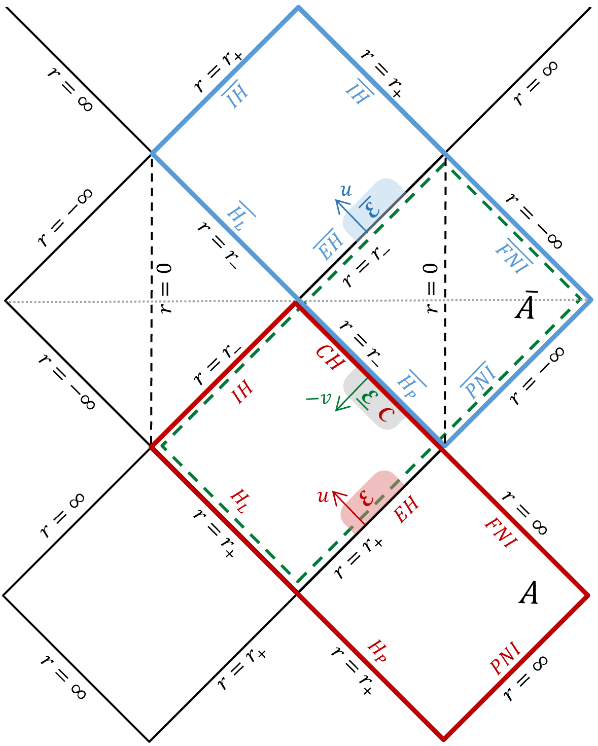
Figure 1: Penrose diagram of (part of) the analytically-extended Kerr geometry. The two types of external universes are marked by $A$ (“usual” universe) and $\overline{A}$ (“negative-mass” universe). EH (IH) marks the ordinary event (inner) horizon, whereas $\overline{EH}$ ($\overline{IH}$) is the event (inner) horizon of the analogous $\overline{A}$-universe BH. The standard Unruh-state domain is bounded by the red frame. The domain for the $\overline{U}$ state (associated with $\overline{A}$) is framed in blue, and its time-reversal image (the $\underline{U}$-state domain) is the region bounded by the green dashed frame. $\mathcal{E}$ (red shaded area) denotes the internal near-EH region, $\mathcal{\overline{E}}$ (blue shaded area) its near-$\overline{EH}$ counterpart, and $\mathcal{\underline{E}}$ (grey shaded area) the time-reversal image of $\mathcal{\overline{E}}$. $\mathcal{\underline{E}}$ coincides with $\mathcal{C}$, which denotes the CH vicinity.

The Unruh state is thus regular throughout the interior of the red frame, and in particular at the EH, which implies $\left\langle T_{uu}\right\rangle_{\text{ren}}^{U}=0$ there [32].

Each mode contributes individually to the fluxes. In Appendix B of Ref. (HTPFinKerr:2022, ), we constructed the “bare” mode-sum expression (namely, prior to regularization) for the Unruh fluxes, $\left\langle T_{uu}\right\rangle_{\text{bare}}^{U}$ and $\left\langle T_{vv}\right\rangle_{\text{bare}}^{U}$, evaluated at the CH and EH.

To express the results compactly, we hereby introduce the summation/integration operator

$$\hat{\sum}_{\pm}\left(\dots\right)\equiv\hbar\int_{0}^{\infty}\sum_{l=0}^{\infty}\sum_{m=-l}^{l}\frac{\left[S_{lm}^{\omega}\left(\theta\right)\right]^{2}}{8\pi^{2}\left(r_{\pm}^{2}+a^{2}\right)}\left(\dots\right)\text{d}\omega\,.$$

Hereafter, a superscript “-” (“+”) in $T_{uu}^{\pm}$ or $T_{vv}^{\pm}$ denotes the CH (EH) limit, particularly referring to evaluation in the shaded region marked $\mathcal{\mathcal{C}}$ ($\mathcal{E})$ in Fig. 1, taking the $r\to r_{-}$ ($r_{+}$) limit therein .

We concentrate now on $\left\langle T_{vv}^{-}\right\rangle_{\text{ren}}^{U}$, leaving $\left\langle T_{uu}^{-}\right\rangle_{\text{ren}}^{U}$ to be treated afterwards. We may write $\left\langle T_{vv}^{-}\right\rangle_{\text{bare}}^{U}=\hat{\sum}_{-}E_{vv\left(\omega lm\right)}^{U-}$, with $E_{vv\left(\omega lm\right)}^{U-}$ given by (see Eq. (B49) in (HTPFinKerr:2022, )):

$$E_{vv\left(\omega lm\right)}^{U-}=\frac{\omega_{-}^{2}}{\omega_{+}}\left[\coth\hat{\omega}_{+}\bigl{(}\left|A_{\omega lm}\right|^{2}+\left|\rho_{\omega lm}^{\text{up}}\right|^{2}\left|B_{\omega lm}\right|^{2}\bigr{)}+\right.$$ (7)

$$\left.2\text{cosech}\,\hat{\omega}_{+}\,\Re\left(\rho_{\omega lm}^{\text{up}}A_{\omega lm}B_{\omega lm}\right)+\bigl{(}1-\left|\rho_{\omega lm}^{\text{up}}\right|^{2}\bigr{)}\left|B_{\omega lm}\right|^{2}\right]$$

where $\hat{\omega}_{\pm}\equiv\pi\omega_{\pm}/\kappa_{\pm}$, $\kappa_{\pm}=\left(r_{+}-r_{-}\right)/4Mr_{\pm}$ and $\rho_{\omega lm}^{\text{up}}$ is the up mode reflection coefficient (see e.g. (HTPFinKerr:2022, )).

Later we shall also need $\left\langle T_{uu}^{+}\right\rangle_{\text{bare}}^{U}$, given by (see Eq. (B45) in (HTPFinKerr:2022, ))

$$\left\langle T_{uu}^{+}\right\rangle_{\text{bare}}^{U}=\hat{\sum}_{+}E_{uu\left(\omega lm\right)}^{U+}\,,\,\,\,E_{uu\left(\omega lm\right)}^{U+}=\omega_{+}\coth\hat{\omega}_{+}\,.$$ (8)

The negative-mass universe.

The entire construction given above for the Unruh state was based in the red frame, corresponding to the “usual” asymptotically flat universe $A$. We now shift to the other asymptotically flat universe, marked by $\overline{A}$ in Fig. 1, and attempt to use it as a basis for constructing an analogous Unruh-like state.

In this universe $\overline{A}$, the value of $r$ steadily decreases going outside, and it approaches $r\to-\infty$ at spacelike (and null) infinity, rather than $+\infty$. Wishing to treat $\overline{A}$ as we treat “conventional” asymptotically-flat universes (like $A$), we transform to a new radial coordinate $\overline{r}\equiv-r$. The new metric then takes exactly the same form as the original metric (1), with $r$ replaced by $\overline{r}$ and $M$ by the negative mass parameter $\overline{M}\equiv-M$. A far observer ($|r|\gg M)$ in this external universe will be gravitationally repelled by the central object. We shall therefore refer to $\overline{A}$ as the negative-mass universe. We denote the future- (past-) null infinity of $\overline{A}$ by $\overline{FNI}$ ($\overline{PNI}$), see Fig. 1.

This universe $\overline{A}$ has two important features distinguishing it from the standard universe $A$: (i) The “ring singularity”, located at $r=0$ (and $\theta=\pi/2$), and (ii) the presence of closed timelike curves (CTCs). We shall return to address these aspects later on. Nevertheless, the negative-mass universe shares various properties with $A$. Most remarkably, it admits its own black hole, whose event horizon is the null curve denoted by $\overline{EH}$ (see Fig. 1): All points to the bottom-right of this null hypersurface can signal to $\overline{FNI}$ (along causal curves), whereas all points to its top-left cannot. Furthermore, the inverse metric component $g^{\overline{r}\,\overline{r}}$ changes sign at two $\overline{r}$ values given by the standard formula $\overline{r_{\pm}}=\overline{M}\pm(\,\overline{M}^{2}-a^{2})^{1/2}$. (The coordinate $\overline{r}$ is therefore timelike at $\overline{r_{-}}<\overline{r}<\overline{r_{+}}$ and spacelike elsewhere.) Notice that $\overline{r_{\pm}}=-r_{\mp}$. Summarizing, the $\overline{A}$-universe event (inner) horizon, denoted $\overline{EH}$ ($\overline{IH}$) in Fig. 1, is located at $\overline{r}=\overline{r_{+}}$ ($\overline{r_{-}}$), which corresponds to $r=r_{-}$ ($r_{+}$).

The $\overline{U}$ and $\underline{U}$ states.

The entire construction of the Unruh state may be repeated analogously in the blue frame (see Fig. 1). That is, while the original Unruh state is fed by initial conditions along the null hypersurfaces PNI and $H_{P}\cup H_{L}$, the new state, hereafter denoted by $\overline{U}$, is fed by fully analogous initial conditions along the corresponding null hypersurfaces $\overline{PNI}$ (where $\overline{r}\to\infty$) and $\overline{H_{P}}\cup\overline{H_{L}}$ (where $\overline{r}=\overline{r_{+}}$ ): bearing positive Eddington frequencies along $\overline{PNI}$, and positive Kruskal frequencies (Unruh:1976, ) along $\overline{H_{P}}\cup\overline{H_{L}}$. It thus functions like the original Unruh state, but with respect to the “barred”, negative-mass, universe $\overline{A}$ (rather than $A$).

The presence of CTCs in the domain $r_{-}>r>-\infty$ (as well as a ring singularity at $r=0$) may challenge the construction of a quantum state in the blue frame. Indeed, there is no well defined Cauchy evolution for initial data specified at $\overline{PNI}$ and $\overline{H_{P}}\cup\overline{H_{L}}$. Note, however, that the field separability provides an alternative framework for defining the evolution: One can decompose the initial data into separable field modes, and then evolve each mode independently (by solving its radial equation). The evolution of each mode is well defined throughout the blue frame. To see this, it is sufficient to note that the potential $V_{\omega lm}\left(r\right)$ is regular at $r=0$ (indeed, on the entire $r$-axis, see (Sup, )). We may use this modewise scheme to uniquely evolve the field modes throughout the blue frame, and thereby construct our $\overline{U}$ state. (Note that even in the ordinary Unruh state the computation of the fluxes is usually done by summing/integrating over the individual modes’ contributions – which can be done also for the $\overline{U}$ state without obstacles.)

We now focus on the blue shaded region right above $\overline{EH}$ in Fig. 1, denoted $\mathcal{\overline{E}}$, which is the “barred” counterpart of $\mathcal{E}$. We wish to compute the $\overline{U}$-state $\left\langle T_{uu}\right\rangle_{\text{bare}}$ in this near-$\overline{EH}$ domain. The mode-sum computation (carried out in (HTPFinKerr:2022, )) that eventually led to Eq. (8), equally applies to the $\overline{U}$-state in the blue frame: One just needs to replace $M$ by $-M$; and, since $\left\langle T_{uu}\right\rangle_{\text{bare}}$ is now evaluated at $\overline{EH}$ (rather than EH), $r_{+}$ is replaced by $r_{-}$. This results in changing $\Omega_{+}\mapsto\Omega_{-}$ and $\kappa_{+}\mapsto\kappa_{-}$ , and, consequently, also $\omega_{+}\mapsto\omega_{-}$ and $\hat{\omega}_{+}\mapsto\hat{\omega}_{-}$. The $U\mapsto\overline{U},\mathcal{E}\mapsto\mathcal{\overline{E}}$ counterpart of Eq. (8) therefore reads

$$\langle T_{uu}^{(\mathcal{\overline{E}})}\rangle_{\text{bare}}^{\overline{U}}=\hat{\sum}_{-}E_{uu\left(\omega lm\right)}^{\overline{U}(\mathcal{\overline{E}})}\,,\,\,\,E_{uu\left(\omega lm\right)}^{\overline{U}(\mathcal{\overline{E}})}=\omega_{-}\coth\hat{\omega}_{-}\,.$$ (9)

The superscript $(\mathcal{\overline{E}})$ marks the specific location of evaluation. Moreover, note that the same regularity argument that led to $\left\langle T_{uu}^{+}\right\rangle_{\text{ren}}^{U}=0$, now implies $\langle T_{uu}^{(\mathcal{\overline{E}})}\rangle_{\text{ren}}^{\overline{U}}=0$ (since $\overline{EH}$ is enclosed by the blue frame).

Finally, we perform a time-reversal transformation of the “barred” universe and the $\overline{U}$ state based on it. This acts as mirroring through the horizontal dotted line in Fig. 1, and takes the blue frame to the dashed green frame therein, where we define the $\underline{U}$ state as the time reversal of the $\overline{U}$ state. In particular, $\mathcal{\overline{E}}$ is mapped to the grey shaded region $\mathcal{\underline{E}}$, just below CH. This is the main region of interest for our computation, since it coincides with the near-CH domain $\mathcal{C}$, as seen in Fig. 1. This time reversal takes the $u$ direction in $\mathcal{\overline{E}}$ to the $-v$ direction in $\mathcal{\underline{E}}$ (as indicated by the blue arrow in $\mathcal{\overline{E}}$ which is mapped to the green arrow in $\mathcal{\underline{E}}$). The $\overline{U}$-state $T_{uu}$ in $\mathcal{\overline{E}}$ (given in Eq. (9)) then matches the $\underline{U}$-state $T_{vv}$ in $\mathcal{\underline{E}}=\mathcal{C}$, namely:

$$\left\langle T_{vv}^{-}\right\rangle_{\text{bare}}^{\underline{U}}=\hat{\sum}_{-}E_{vv\left(\omega lm\right)}^{\underline{U}-}\,,\,\,\,E_{vv\left(\omega lm\right)}^{\underline{U}-}=\omega_{-}\coth\hat{\omega}_{-}\,;$$ (10)

and, similarly,

$$\left\langle T_{vv}^{-}\right\rangle_{\text{ren}}^{\underline{U}}=\langle T_{uu}^{(\mathcal{\overline{E}})}\rangle_{\text{ren}}^{\overline{U}}=0$$ (11)

(the rightmost equality was already established above).

Regularization.

We now apply the procedure of regularization by subtracting the $\underline{U}$-state from the Unruh state, recalling that the difference between the bare mode-sums of the two states is regular, and equals the difference between the renormalized quantities. That is,

$$\left\langle T_{vv}^{-}\right\rangle_{\text{ren}}^{U}-\left\langle T_{vv}^{-}\right\rangle_{\text{ren}}^{\underline{U}}=\hat{\sum}_{-}\left(E_{vv\left(\omega lm\right)}^{U-}-E_{vv\left(\omega lm\right)}^{\underline{U}-}\right)\,.$$

Recalling Eqs. (10,11), our final expression for $\left\langle T_{vv}^{-}\right\rangle_{\text{ren}}^{U}$ is thus

$$\left\langle T_{vv}^{-}\right\rangle_{\text{ren}}^{U}=\hat{\sum}_{-}\left(E_{vv\left(\omega lm\right)}^{U-}-\omega_{-}\coth\hat{\omega}_{-}\right)\,,$$ (12)

where $E_{vv\left(\omega lm\right)}^{U-}$ was specified in Eq. (7), and, recall $\hat{\omega}_{\pm}\equiv\pi\omega_{\pm}/\kappa_{\pm}$.

Finally, we consider $\left\langle T_{uu}^{-}\right\rangle_{\text{ren}}^{U}$. In Eq. (B51) in (HTPFinKerr:2022, ) we found the difference:

$$\left\langle T_{uu}^{-}\right\rangle_{\text{ren}}^{U}-\left\langle T_{vv}^{-}\right\rangle_{\text{ren}}^{U}=$$ (13)

$$\hat{\sum}_{-}\omega_{-}\left(\coth\hat{\omega}_{+}-1\right)\left(1-\left|\rho_{\omega lm}^{\text{up}}\right|^{2}\right)\,,$$

which, along with Eq. (12), yields $\left\langle T_{uu}^{-}\right\rangle_{\text{ren}}^{U}$.

We have thus obtained simple and useful expressions for $\left\langle T_{vv}^{-}\right\rangle_{\text{ren}}^{U}$ and $\left\langle T_{uu}^{-}\right\rangle_{\text{ren}}^{U}$.

Numerical results.

Next we numerically compute $\left\langle T_{vv}^{-}\right\rangle_{\text{ren}}^{U}$ and $\left\langle T_{uu}^{-}\right\rangle_{\text{ren}}^{U}$ based on Eqs. (12),(13).

We start at the pole, where only $m=0$ modes contribute (since $S_{l,m\neq 0}^{\omega}\left(\theta=0\right)$ vanishes), which drastically simplifies the numerical application. We numerically compute $A_{\omega lm},B_{\omega lm},\rho_{\omega lm}^{\text{up}}$ and construct the integrand in Eq. (12) (see (Sup, ) for details). We find that all divergences present in $\left\langle T_{vv}^{-}\right\rangle_{\text{bare}}^{U}$ entirely disappear in its renormalized counterpart. This provides a crucial test for our state-subtraction procedure. In fact, the integrand converges exponentially in both $l$ and $\omega$.

Fig. (2) portrays $\left\langle T_{vv}^{-}\right\rangle_{\text{ren}}^{U}$ and $\left\langle T_{uu}^{-}\right\rangle_{\text{ren}}^{U}$ at the pole versus $a/M$.

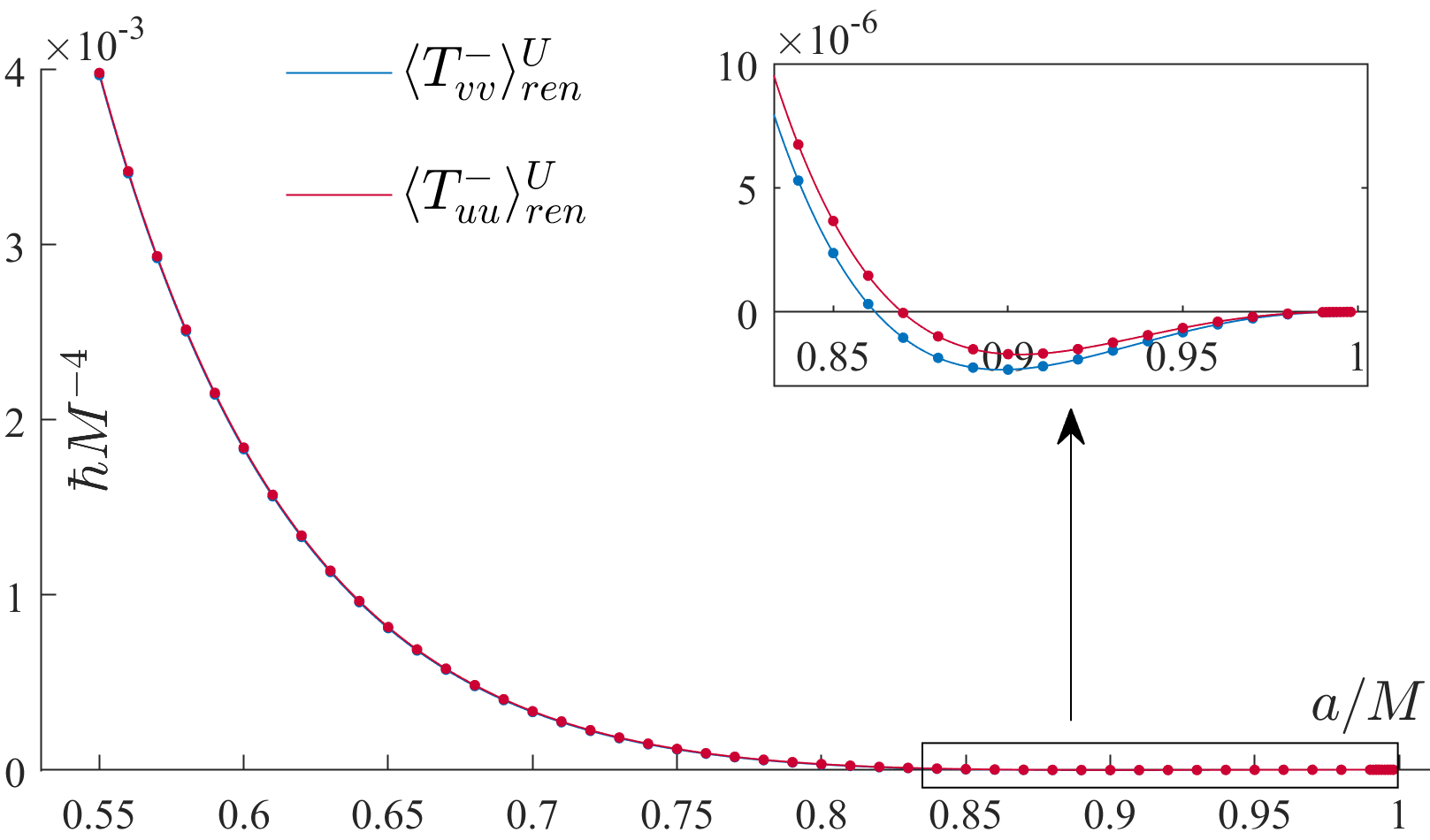
Figure 2: The polar CH-limit Unruh fluxes versus $a/M$, with the sign-flip domain zoomed-in at the top-right corner. The dots were numerically computed, while the connecting lines are interpolated. Note that wherever only the red is visible, it covers the blue.

It would be desirable to compare our results with those obtained by other regularization methods. For the specific cases $a/M=0.8$ and $0.9$, we computed (future, ) the polar fluxes via point splitting (Christensen:1976, ) for various $r_{-}<r<r_{+}$ values. We then evaluated the $r\to r_{-}$ limit of these fluxes (see (Sup, )). We find full agreement between the two methods (point splitting and state subtraction). E.g., for $a/M=0.8$, both methods yield $\left\langle T_{vv}^{-}\right\rangle_{\text{ren}}^{U}\approx 0.00003013\,\hbar M^{-4}$ and $\left\langle T_{uu}^{-}\right\rangle_{\text{ren}}^{U}\approx 0.00003232\,\hbar M^{-4}$ . This excellent agreement strongly corroborates our state-subtraction method.

It is interesting to compare the features seen here to the analogous RN case (FluxesRN:2020, ). The CH-limit polar fluxes in Kerr, like in RN (with $Q/M$ replacing $a/M$), are increasingly positive for smaller spin values. They decrease with increasing $a/M$ and change their sign at some critical value beyond which they are negative all the way to their decay at $a/M\to 1$ (more details in (Sup, )). The critical sign-flip values are smaller here compared to their RN counterparts (FluxesRN:2020, ), being $a/M\approx 0.862$ for $\left\langle T_{vv}^{-}\right\rangle_{\text{ren}}^{U}$ and $\approx 0.870$ for $\left\langle T_{uu}^{-}\right\rangle_{\text{ren}}^{U}$. Moreover, numerically investigating the mentioned near-extremal decay versus the small parameter $\epsilon\equiv\sqrt{1-\left(a/M\right)^{2}}$ we obtain that, in full analogy with the RN case (FluxesRNext:2021, ), $\left\langle T_{vv}^{-}\right\rangle_{\text{ren}}^{U}\propto\epsilon^{4}$ and $\left\langle T_{uu}^{-}\right\rangle_{\text{ren}}^{U}\propto\epsilon^{5}$ (see (Sup, )).

Next, we compute the fluxes at other $\theta$ values, for $a/M=0.8$. We again find exponential convergence of the integrand in both $l$ and $\omega$ – supporting the validity of our regularization method off-pole as well. Fig. 3 displays our results. Interestingly, the CH-limit fluxes change their sign twice as a function of $\theta$ until they peak at the equator (around which they are symmetric).

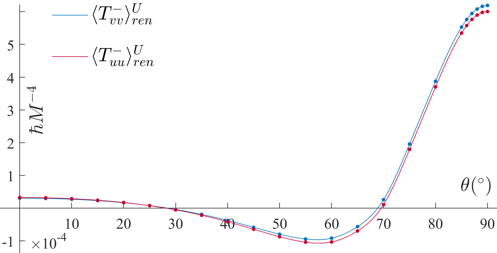
Figure 3: The CH-limit Unruh fluxes versus $\theta$, for $a/M=0.8$. The dots were numerically computed and the connecting lines are interpolated.

Conclusion.

We computed the semiclassical Unruh-state fluxes $\left\langle T_{uu}\right\rangle_{\text{ren}}$ and $\left\langle T_{vv}\right\rangle_{\text{ren}}$ at the CH of a spinning BH, using the state-subtraction method. We found generically nonvanishing $\left\langle T_{vv}\right\rangle_{\text{ren}}$ at the CH, implying the divergence of the RSET (and tidal forces) there. Furthermore, we found that these fluxes may be positive or negative, depending on $a/M$ and $\theta$. The sign of these fluxes may be crucial for the nature of backreaction (see Introduction).

The quantum state $\underline{U}$ used for this subtraction is nonconventional in several respects: First, it (partly) resides in the “negative mass” asymptotic universe $\overline{A}$ in the analytically extended Kerr geometry – a spacetime region whose existence in a real spinning BH is at least highly questionable. Second, it is a time-reversed quantum state (with asymptotic boundary data specified on the future rather than past null infinity of $\overline{A}$). Third, this universe $\overline{A}$ contains CTCs as well as a naked ring singularity. Nevertheless, we use the subtraction of this quantum state merely as a mathematical-computational tool and it seems to work extremely well: First, it fully regularizes the flux mode-sums. Furthermore, the subtracted mode-sum converges exponentially fast, in both $\omega$ and $l$. Moreover, in two specific cases, we compared the resultant flux values to those obtained by point splitting, and found excellent quantitative agreement.

It will be important to extend this research to additional $a/M$ values (especially off-pole, where it would also be imperative to compare to other methods) – and, even more importantly, to the more realistic (quantum) electromagnetic field.

Computing the semiclassical fluxes at the CH of a Kerr BH (and, more importantly, determining their sign) is a major feat, but definitely does not mark the end of this research: Rather, these results open a door to the study of backreaction (via the semiclassical Einstein equation) – and the resultant spacetime structure – inside a realistic, evaporating, spinning BH. We hope to further explore this issue in a future work.

- (1) B. Carter, Complete Analytic Extension of the Symmetry Axis of Kerr’s Solution of Einstein’s Equations, Phys. Rev. 141, 1242 (1966).
- (2) J. C. Graves and D. R. Brill, Oscillatory Character of Reissner-Nordström Metric for an Ideal Charged Wormhole, Phys. Rev. 120, 1507 (1960).
- (3) A. Ori, Structure of the singularity inside a realistic rotating black hole, Phys. Rev. Lett. 68, 2117 (1992).
- (4) M. Dafermos and J. Luk, The interior of dynamical vacuum black holes I: The -stability of the Kerr Cauchy horizon, arXiv:1710.01722.
- (5) F. J. Tipler, Singularities in conformally flat spacetimes, Phys. Lett. A 64, 8 (1977).
- (6) A. Ori, Strength of curvature singularities, Phys. Rev. D 61, 064016 (2000).
- (7) P. R. Brady, S. Droz, and S. M. Morsnik, Late-time singularity inside nonspherical black holes, Phys. Rev. D. 58, 084034 (1998).
- (8) A. Ori, Oscillatory null singularity inside realistic spinning black holes, Phys. Rev. Lett. 83, 5423 (1999).
- (9) W. A. Hiscock, Stress-energy tensor near a charged, rotating, evaporating black hole, Phys. Rev. D. 15, 3054 (1977).
- (10) N. D. Birrell and P. C. W. Davies, On falling through a black hole into another universe, Nature (London) 272, 35 (1978).
- (11) W. A. Hiscock, Quantum-mechanical instability of the Kerr-Newman black-hole interior, Phys. Rev. D. 21, 2057 (1980).
- (12) A. C. Ottewill and E. Winstanley, Renormalized stress tensor in Kerr space-time: General results, Phys. Rev. D. 62, 084018 (2000).
- (13) N. Zilberman, A. Levi and A. Ori, Quantum Fluxes at the Inner Horizon of a Spherical Charged Black Hole, Phys. Rev. Lett. 124, 171302 (2020).
- (14) S. M. Christensen, Vacuum expectation value of the stress tensor in an arbitrary curved background: The covariant point separation method, Phys. Rev. D. 14, 2490 (1976).
- (15) N. Zilberman, A. Ori, Quantum fluxes at the inner horizon of a near-extremal spherical charged black bole, Phys. Rev. D. 104, 024066.
- (16) S. Hollands, R. M. Wald and J. Zahn, Quantum instability of the Cauchy horizon in Reissner-Nordström-deSitter spacetime, Class. Quant. Grav. 37, 115009 (2020).
- (17) S. Hollands, C. Klein and J. Zahn, Quantum stress tensor at the Cauchy horizon of the Reissner-Nordström-de Sitter spacetime, Phys. Rev. D. 102(8), 085004 (2020).
- (18) P. Candelas, Vacuum polarization in Schwarzschild spacetime, Phys. Rev. D. 21, 2185 (1980).
- (19) S. M. Christensen and S. A. Fulling, Trace anomalies and the Hawking effect, Phys. Rev. D. 15(8), 2088 (1977).
- (20) P. Taylor, Regular Quantum States on the Cauchy Horizon of a Charged Black Hole, Class. Quant. Grav. 37, 045004 (2020).
- (21) B. Carter, Hamilton-Jacobi and Schrödinger separable solutions of Einstein’s equations, Comm. Math. Phys. 10(4), 280-310 (1968).
- (22) S. A. Teukolsky, Rotating Black Holes: Separable Wave Equations for Gravitational and Electromagnetic Perturbations, Phys. Rev. Lett. 29, 1114 (1972).
- (23) C. Flammer, Spheroidal wave functions, Stanford University Press, Stanford, California (1957).
- (24) W. G. Unruh, Notes on black-hole evaporation, Phys. Rev. D. 14, 870 (1976).
- (25) N. Zilberman, M. Casals, A. Ori, and A. C. Ottewill, Two-point function of a quantum scalar field in the interior region of a Kerr black hole, arXiv:2203.07780 (accepted for publication in Phys. Rev. D).
- (26) N. Zilberman, M. Casals, A. Ori, and A. C. Ottewill, in preperation.
- (27) M. Sasaki and H. Tagoshi, Analytic Black Hole Perturbation Approach to Gravitational Radiation, Liv. Rev. Rel. 6, 6 (2003).
- (28) Black Hole Perturbation Toolkit, (bhptoolkit.org).
- (29) A. Levi, Renormalized stress-energy tensor for stationary black holes, Phys. Rev. D. 95, 025007 (2017).
- (30) A. Levi, E. Eilon, A. Ori and M. van de Meent, Renormalized Stress-Energy Tensor of an Evaporating Spinning Black Hole, Phys. Rev. Lett. 118, 141102 (2017).
- (31) See Supplemental Material for the effective potential (section 1), basic details on the numerical implementation (section 2), the point-splitting flux values at the IH limit (section 3) and the near-extremal domain (section 4). The Supplemental Material includes Refs. (FluxesRN:2020, ; Christensen:1976, ; FluxesRNext:2021, ; HTPFinKerr:2022, ; future, ; Sasaki-Tagoshi, ; BHPT, ; LeviRSET:2017, ; LeviEilonOriMeent:2017, ).