Comparing the frequentist and Bayesian periodic signal detection: rates of statistical mistakes and sensitivity to priors

Abstract

We perform extensive Monte Carlo simulations to systematically compare the frequentist and Bayesian treatments of the Lomb–Scargle periodogram. The goal is to investigate whether the Bayesian period search is advantageous over the frequentist one in terms of the detection efficiency, how much if yes, and how sensitive it is regarding the choice of the priors, in particular in case of a misspecified prior (whenever the adopted prior does not match the actual distribution of physical objects). We find that the Bayesian and frequentist analyses always offer nearly identical detection efficiency in terms of their tradeoff between type-I and type-II mistakes. Bayesian detection may reveal a formal advantage if the frequency prior is nonuniform, but this results in only $\sim 1$ per cent extra detected signals. In case if the prior was misspecified (adopting nonuniform one over the actual uniform) this may turn into an opposite advantage of the frequentist analysis. Finally, we revealed that Bayes factor of this task appears rather overconservative if used without a calibration against type-I mistakes (false positives), thereby necessitating such a calibration in practice.

1 Introduction

Periodogram is a tool that enables the detection of periodic variations in time series data, a widespread astronomical task. Speaking more accurately, it is a collection of tools, because multiple periodograms were constructed so far. The earliest one is the classic periodogram, also known as the Schuster periodogram (Schuster, 1898). It originates from a direct estimation of the power spectrum.

However, another type of periodograms became more widespread in astronomy, known as the Lomb (1976) – Scargle (1982) periodogram (LSP hereafter). It is a representative of an alternative approach based on the least squares spectral analysis (LSSA), or the Vaníček method (Vaníček, 1969). Unlike the Schuster periodogram, the LSP was not defined through the power spectrum (even though it can be used as such an estimate if necessary). Rather, it was defined through the least squares fit of the data using a sinusoidal model.

One reason why the LSP appeared so popular in astronomical applications (perhaps contrary to the Schuster periodogram) is flexibility of the LSSA behind it. Periodograms of this type can be easily generalized to include more complicated models. In particular, Ferraz-Mello (1981) introduced the so-called date-compensated discrete Fourier transform (DCDFT) that involves an internally fittable constant offset (not present in the initial LSP). Now it is also known as the generalized LSP (or GLSP), thanks to the efficient computing algorithm by Zechmeister & Kürster (2009). Cumming et al. (1999) considered more extensions of this type taking into account linear or polynomial trends. Further ways to generalize the LSP involve the use of nonsinusoidal and/or nonlinear models of the periodic signal, multicomponent signals, as well as more complicated noise models, including even Gaussian processes, see (Baluev, 2014) for a review and (Baluev, 2009a, b, 2013a, 2013b, 2015a) as particular examples.

All these generalizations of the LSP refer to the frequentist analysis. A yet another branch of period search tools is based on the Bayesian treatment of a periodogram. There are two main ways how the Bayesian periodograms were introduced in the literature. The first one is due to Bretthorst (2001a, b), who defined the Bayesian LS periodogram (or BLSP) through the posterior frequency distribution. This approach was further developed by Mortier et al. (2014) who added a free offset to the model, just like in the DCDFT/GLSP, so their method is called as the Bayesian GLSP (BGLSP).

The second way to construct a Bayesian periodogram follows from Cumming (2004), and it is based on the Bayes factor (or a close entity like the posterior odds ratio) of the corresponding signal detection task, rather than on the posterior frequency distribution.

Two flavors of a Bayesian periodogram mentioned above are not necessarily equivalent, because the Bayes factor is deemed to solve the signal detection task (basically, determination of an absolute ordinate scale for a periodogram), while the posterior frequency distribution targets the aliasing ambiguity task (relative intercomparison of peaks in the same periodogram). In this study we focus on the signal detection, which is more basic with respect to the aliasing (before resolving possibly ambiguous frequency, we should demonstrate that some periodic signal is likely to exist). Therefore, we assume from the beginning that our Bayesian periodogram is based on the Bayes factor.

Bayesian periodograms, just like Bayesian analysis in general, are usually believed to offer some advantages over the classic frequentist ones. In particular, they offer an easy way to take into account prior information, if it is available in the form of a more or less accurately defined distribution. From the other side, they have an obvious practical disadvantage because of high computing demands. Computation of a frequentist periodogram may be slow sometimes, maybe not too much faster than Markov Chain Monte Carlo (MCMC) typically used to sample a posterior distribution. However, Bayes factor computation is more challenging than MCMC. Therefore, an important practical question is raised: do the Bayesian periodograms actually offer an advantage worthy of the sacrificed computing speed? For example, do they offer a better detection efficiency, and if yes then how valuable this advantage is? And is it stable with respect to input conditions like time series sampling, amount of data, adopted priors, etc? These questions are often avoided in practice, because different works usually tend to apply a particular selected method to a particular practical task. However, to gain a more or less completed picture it is necessary to test two rival approaches systematically, under varying conditions, but always using an equivalent treatment for them both. Here our aim is to perform such a comparison, based on numerical simulations.

One recent example of such a study, employing a good-practice comparison, was provided by the exoplanets detection challenge by Nelson et al. (2020). However, this work was focused, mostly, on the intercomparison of different Bayesian methods, mainly considering the stability of the computed Bayesian evidence. The detection efficiency for Bayesian and frequentist methods was not considered in an equivalent and comparative treatment. Additionally, this challenge targeted more complicated data models developed for a more specific task of exoplanets detection. Our goal here is to consider a wider-purpose formulation of the period search task.

The plan of the paper is as follows. In Sect. 2 we present an introductory discussion about the general relationship between Bayesian and frequentist analyses, how they may be formally compared, and how this applies to periodograms. In Sect. 3 we present the details of our Monte Carlo simulations, while the results of these simulations are presented in Sect. 4. Most of these results are presented in graphical form, but in the printed paper we provide only a portion of the plots for demonstrative purposes. The full set of graphs is attached as the online-only material (see App. D).

2 Bayesian vs. frequentist treatments of the periodogram

2.1 Relationship between Bayesian and frequentist model checking

Bayesian and frequentist analysis differ from each other at multiple layers, starting from the philosophical understanding of probability (Gelman, 2008). Of course, a complete review of the issue is out of the scope here, because our main goal is to investigate a particular task of periodic signal detection. Still there are practical aspects that we need to compare in a more general context to avoid certain misconceptions.

In Bayesian model selection we deal with the so-called evidence:

$$E_{\rm B}(\mn@boldsymbol{x}|\mathcal{M},\mathcal{W})=\int L(\mn@boldsymbol{x}|\mn@boldsymbol{\theta},\mathcal{M})\mathcal{W}(\mn@boldsymbol{\theta})d\mn@boldsymbol{\theta},$$ (1)

where $L$ is the likelihood, i.e. the p.d.f. of the data $\mn@boldsymbol{x}$ given the model $\mathcal{M}$ and its parameters $\mn@boldsymbol{\theta}$. The weight function $\mathcal{W}(\mn@boldsymbol{\theta})\geq 0$ is the prior p.d.f. for $\mn@boldsymbol{\theta}$.

The evidence $E_{B}$ is also known under other titles: prior predictive, average likelihood, marginal likelihood. In fact, it represents the p.d.f. of the data $\mn@boldsymbol{x}$, treated conditionally to the adopted model and to the adopted prior $\mathcal{W}$.

The ratio of two Bayesian evidences like (1), computed for two alternative models is called the Bayes factor

$$R_{\rm B}(\mn@boldsymbol{x})=\frac{E_{\rm B}(\mn@boldsymbol{x}|\mathcal{M}_{2},\mathcal{W}_{2})}{E_{\rm B}(\mn@boldsymbol{x}|\mathcal{M}_{1},\mathcal{W}_{1})}.$$ (2)

It usually serves as a key quantity for Bayesian model selection (e.g. Bayarri & Berger, 2013).

In the frequentist hypothesis testing we usually deal with ratios of likelihood maxima that refer to our rival models. In this case we should first define the quantity

$$E_{\rm F}(\mn@boldsymbol{x}|\mathcal{M},\Theta)=\max_{\mn@boldsymbol{\theta}\in\Theta}L(\mn@boldsymbol{x}|\mn@boldsymbol{\theta},\mathcal{M}),$$ (3)

where $\Theta$ is some a priori specified domain, in which $\mn@boldsymbol{\theta}$ is supposed to always reside. The maximum likelihood, $E_{\rm F}$, plays now the same key role as the evidence $E_{\rm B}$ served in Bayesian analysis. Therefore, we may alternatively call it the “frequentist evidence”. And analogously to Bayesian case, we can define the ratio of two rival evidences which now turns into the classic likelihood ratio:

$$R_{\rm F}(\mn@boldsymbol{x})=\frac{E_{\rm F}(\mn@boldsymbol{x}|\mathcal{M}_{2},\Theta_{2})}{E_{\rm F}(\mn@boldsymbol{x}|\mathcal{M}_{1},\Theta_{1})}.$$ (4)

We can see that $R_{\rm F}$ apparently disallows to include any detailed prior distribution (in form of a weight function). This is a point the frequentist approach is sometimes criticized for, because $R_{\rm B}$ just looks more versatile and offers more control through $\mathcal{W}_{1,2}$. But simultaneously it is neither true that frequentist approach ignores any prior information at all (there is a prior domain $\Theta$), nor that it assumes any specific prior in Bayesian sense (because $E_{\rm F}$ is not simply a restriction of $E_{\rm B}$ to any specific prior).

From a practical point of view, Bayesian and frequentist approaches are constructively similar, but differ in their target metric, either $E_{\rm B}$ or $E_{\rm F}$. The first one is based on averaging, while the second one relies on optimization. But let us now consider the following “generalized evidence”:

$$E_{p}(\mn@boldsymbol{x}|\mathcal{M},\mathcal{W})=\left(\int\left[L(\mn@boldsymbol{x}|\mn@boldsymbol{\theta},\mathcal{M})\right]^{p}\mathcal{W}(\mn@boldsymbol{\theta})d\mn@boldsymbol{\theta}\right)^{\frac{1}{p}}.$$ (5)

This is simply the $L_{p}$-norm of the likelihood. Now we can see that both $E_{\rm B}$ and $E_{\rm F}$ represent two limiting cases of $E_{p}$:

$$E_{\rm B}(\mn@boldsymbol{x}|\mathcal{M},\mathcal{W}) = E_{1}(\mn@boldsymbol{x}|\mathcal{M},\mathcal{W}),$$

$$E_{\rm F}(\mn@boldsymbol{x}|\mathcal{M},\Theta) = E_{\infty}(\mn@boldsymbol{x}|\mathcal{M},\mathcal{W}),\quad\Theta={\rm supp}(\mathcal{W}).$$ (6)

And based on the generalized $L_{p}$-evidence (5), the Bayes factor (2) is generalized to

$$R_{p}(\mn@boldsymbol{x})=\frac{E_{p}(\mn@boldsymbol{x}|\mathcal{M}_{2},\mathcal{W}_{2})}{E_{p}(\mn@boldsymbol{x}|\mathcal{M}_{1},\mathcal{W}_{1})},$$ (7)

so that $R_{\rm B}=R_{1}$ and $R_{\rm F}=R_{\infty}$.

From this position Bayesian and frequentist approaches look entirely as peers. None of the two metric is a worse (or weakened) version of another; rather they are opposite special cases of the same $E_{p}$. They differ from each other just like the $L_{1}$-norm differs from the $L_{\infty}$-norm. This argumentation also helps us to understand better why the $E_{\rm F}$ metric does not apparently allow to specialize any detailed prior. Before passing to the limit $p\to\infty$, the evidence does include $\mathcal{W}$ in its full form, but in the limiting behaviour it appears invariable with respect to it. Setting different $\mathcal{W}$ results in different $E_{\rm B}$, but always leads to the same $E_{\rm F}$, at least if $\Theta$ is unchanged.

If the “generalized evidence” $E_{p}$ looks too artificial, it could be constructed using an alternative more constructive argumentation. Bayesian evidence (1) depends on the prior $\mathcal{W}(\mn@boldsymbol{\theta})$ in the form of a penalty added to the log-likelihood, i.e. as $\log L+\log\mathcal{W}$. However, in an observations-related science nothing can be specified precisely, and so $\mathcal{W}$ may involve uncertainties. In this case we should modify the evidence to take the uncertainty of $\mathcal{W}$ into account. Basically, we should downweight the impact of $\mathcal{W}$, for example as $\log L+\frac{1}{p}\log\mathcal{W}$, where $p\geq 1$. And precisely this type of downweighting is offered by the definition (5). The quantity $p$ attains now the meaning of the prior’s uncertainty. The minimum convex metric has $p=1$, and it corresponds to the pure Bayesian analysis with a strictly specified prior. The frequentist analysis, on the other hand, corresponds to the maximum-uncertainty case with infinite $p$.

Of course, if prior information is sound enough, e.g. if we can formalize our physical knowledge through a well-determined function $\mathcal{W}$, then it looks reasonable to use Bayesian approach, because it can be tuned against this particular $\mathcal{W}$. But we often cannot formalize our knowledge through a well-determined function. In this case, a common Bayesian workaround is to use some non-informative (high-entropy) prior, e.g. wide-range flat one. However, such $\mathcal{W}$ is just a yet another strictly specified prior. It may appear wrong, that is it may mismatch the actual distribution of physical objects that we consider. Consequences of such a mismatch are unclear and need an investigation, at least.

For example, in the task of periodic signal detection it looks physically reasonable to assume a uniform prior for an angular variable like the phase of a sinusoid. Contrary to that, the frequency prior is less obvious, and in fact applications may assume different frequency priors. For example, it can be uniform in terms of the frequency $f$ itself, or in terms of the period $P=1/f$, or in terms of $\log f$. These are three quite different and rather restrictive distributions that may or may not match the distribution of actual objects that we observe. Similar uncertainty appears regarding the prior for the amplitude of a periodic signal.

Summarizing all the above, three primary questions can be formulated: (i) what happens if our adopted Bayesian prior $\mathcal{W}$ mismatches the actual distribution of physical objects, (ii) whether and when the Bayes factor $R_{\rm B}$ becomes advantageous or disadvantageous over the frequentist likelihood ratio $R_{\rm F}$, and (iii) how to measure this possible advantage numerically. However, in this study these questions are to be addressed in view of our practical task, the detection of a periodic signal. In this setting the $\mathcal{M}_{1}$ model refers to noise + possible nuisance background variation, while $\mathcal{M}_{2}$ additionally contains a periodic signal.

2.2 Statistical error rates: why do we need them?

Differences between Bayesian and frequentist treatments are not limited to the use of different statistic, $R_{\rm B}$ or $R_{\rm F}$. The further difference is how these $R$ values are used.

Let us consider the frequentist case first. In general, larger values of the likelihood ratio $R_{\rm F}$ indicate better support in favor of the model $\mathcal{M}_{2}$, over $\mathcal{M}_{1}$. However, the practical numeric threshold of $R_{\rm F}$ is derived from certain post-calibration. This calibration is usually done through the notion of $p$-value, aka false alarm probability (more frequent term in astronomy), aka false positives rate, aka type-I mistake probability. The false alarm probability (${\rm FAP}$) is the probability to obtain, being governed by the threshold rule $R_{\rm F}\geq R_{\rm F}^{*}$, an erroneous decision in favour of $\mathcal{M}_{2}$ while $\mathcal{M}_{1}$ is actually true. Whenever this ${\rm FAP}$ was expressed through a function $\alpha(R_{\rm F}^{*})$, and given some small level $\alpha^{*}$, we may define the threshold $R_{\rm F}^{*}$ from the implicit equation $\alpha(R_{\rm F}^{*})=\alpha^{*}$.

While the type-I mistakes rate provides the required calibration for $R_{\rm F}$, type-II mistakes define another important characteristic, namely the power of the test, or how well it can reveal hidden low-amplitude signals. Given the threshold $R_{\rm F}^{*}$, the type-II mistake is a false non-detection of an existing signal, meaning to accept $\mathcal{M}_{1}$ while $\mathcal{M}_{2}$ is true. The type-II mistakes rate is characterized by another function $\beta(R_{\rm F}^{*})$.

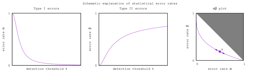
Figure 1: Illustration explaining the $\alpha$ and $\beta$ error rates and the tradeoff between them. The argument $\tau$ stands for the adopted test statistic, either $R_{\rm F}$ or $R_{\rm B}$ or whatever. Notice that $1-\beta$ has the meaning of “true alarm probability”, which should necessarily exceed $\alpha$, at least for a logically reasonable test. So in the $\alpha\beta$ diagram we grayed out the top-right triangle $\alpha+\beta>1$ to reflect this.

Therefore, we ultimately have two univariate functions that jointly characterize error rates of our test: $\alpha(R_{\rm F})$ and $\beta(R_{\rm F})$. The $\alpha$-function is monotonically decreasing, while $\beta$ is monotonically increasing, so the choice of the detection threshold $R_{\rm F}^{*}$ is always governed by the tradeoff between $\alpha$ and $\beta$. In fact, the $R_{\rm F}$ argument becomes now just a dummy variable, so its calibration (absolute scale) is not important in itself. What attains the greatest importance is the implicit relationship between $\alpha$ and $\beta$. 2D diagrams of this type allow us to comprehensively characterize the intrinsic test performance, as shown in Fig. 1. They will be our primary tool to investigate the performance of a signal detection test.

Now let us proceed to Bayesian signal detection. There is a universal empiric scale to interpret $R_{\rm B}$ (Jeffreys, 1998). For example, $R_{\rm B}=1$ means equally supported models, $R_{\rm B}=10$ means substantial evidence in favour of $M_{2}$, $R_{\rm B}=100$ means very strong evidence for $M_{2}$, and so on. Contrary to the frequentist case, we may finish our analysis by computing $R_{\rm B}$, apparently without any need of its calibration. The associated rates of statistical mistakes are then moved out of the focus entirely, and that is why they are often deemed to be a solely frequentist-related tool.

However, even in Bayesian literature it is recognized that without a calibration against the mistakes rates any statistical method (including Bayesian) may appear deficient (Draper, 2013). Any statistical method must be calibrated in the sense that we should have an assessment of how frequently it yields the right answer. And in fact, there is no universal guarantee that Jeffreys’ empiric scale for the Bayes factor remains equally good for any particular task.

Figure 2: Comparison of different tests using the $\alpha\beta$ diagram.

In the setting of our study we should characterize the behaviour of $R_{\rm B}$ using the $\alpha\beta$ diagram, entirely analogously to the frequentist likelihood ratio $R_{\rm F}$. Moreover, the $\alpha\beta$ diagram appears useful to intercompare the performance of such alternative statistical tests, see Fig. 2 for an illustration. To make this comparison a bit more objective, we introduce the following metric:

$$I_{\alpha\beta} = \int\limits_{0}^{1}\beta\,d\alpha=-\int\limits_{\tau_{\min}}^{\tau_{\max}}\beta(\tau)\alpha^{\prime}(\tau)d\tau=$$ (8)

$$= \int\limits_{\tau_{\min}}^{\tau_{\max}}\alpha(\tau)\beta^{\prime}(\tau)d\tau=\int\limits_{0}^{1}\alpha\,d\beta=I_{\beta\alpha},$$

where $\tau$ is our test statistic, either $R_{\rm B}$ or $R_{\rm F}$. Smaller $I_{\alpha\beta}$ implies that we have a smaller integrated rate of type-II mistakes, meaning a more efficient detection in average. So tests with smaller $I_{\alpha\beta}$ are likely more advantageous. Equal values of $I_{\alpha\beta}$ may mean that two methods are either equivalent (third plot of Fig. 2) or their relationship is inconclusive (second plot of Fig. 2).

In this section we cannot bypass a significant practical issue related to the calculation of the $\alpha\beta$ rates. The ${\rm FAP}$, for example, appears to additionally depend on the $\mathcal{M}_{1}$ model parameters:

$${\rm FAP}(\tau^{*}|\mn@boldsymbol{\theta}_{1})=\Pr\{\tau(\mn@boldsymbol{x})>\tau^{*}\,|\,\mn@boldsymbol{\theta}_{1},\mathcal{M}_{1}\}.$$ (9)

The nuisance vector $\mn@boldsymbol{\theta}_{1}$ is a priori unknown, but we need to reduce this ${\rm FAP}$ to an univariate function $\alpha(\tau^{*})$ somehow. A widespread practical workaround of this issue is to substitute the best-fitting estimate $\hat{\mn@boldsymbol{\theta}}_{1}$ in (9). This simplified method is called the “plug-in $p$-value” by (Bayarri & Berger, 2013):

$$\alpha_{\rm plug}(\tau^{*})={\rm FAP}(\tau^{*}|\hat{\mn@boldsymbol{\theta}}_{1}).$$ (10)

This method is obviously flawed because the estimate $\hat{\mn@boldsymbol{\theta}}_{1}$ always has some uncertainty, so the ${\rm FAP}$ resulting from (10) becomes inherently inaccurate. In fact it is a yet another point the frequentist approach is sometimes criticized for, however we can see that this issue is unrelated to the choice of the frequentist or Bayesian detection metric $R_{\rm F}/R_{\rm B}$ and can equally affect the both. Moreover, multiple more neat methods are known well that allow to get rid of the $\mn@boldsymbol{\theta}_{1}$ dependency.

The first approach is now called the supremum method (Bayarri & Berger, 2000), although it was known decades ago (e.g. Koroluk et al., 1985, § 20.5). It requires to maximize the ${\rm FAP}$ over $\mn@boldsymbol{\theta}_{1}$:

$$\alpha_{\rm sup}(\tau^{*})=\max_{\mn@boldsymbol{\theta}_{1}\in\Theta_{1}}{\rm FAP}(\tau^{*}|\mn@boldsymbol{\theta}_{1}).$$ (11)

This method is frequentist-leaned because it is more conservative and allows to keep the number of false positives below the requested $\alpha$ level regardless of the unknown $\mn@boldsymbol{\theta}_{1}$. Therefore, it is a natural solution if placing such a limit on the type-I mistakes is our ultimate goal. A yet another alternative is to average the ${\rm FAP}$ over $\mn@boldsymbol{\theta}_{1}$ using the relevant prior:

$$\alpha_{\rm avg}(\tau^{*})=\int{\rm FAP}(\tau^{*}|\mn@boldsymbol{\theta}_{1})\mathcal{W}_{1}(\mn@boldsymbol{\theta}_{1})d\mn@boldsymbol{\theta}_{1}.$$ (12)

This method is also called the prior predictive p-value (Box, 1980) and it is Bayesian-leaned in some sense. It allows to count the cumulative number of false positives in our survey, provided that $\mathcal{W}_{1}(\mn@boldsymbol{\theta}_{1})$ describes its actual (physical) distribution. This list of possible ways to handle nuisance parameters is incomplete, for example we omitted the posterior predictive p-values.

The error rate $\beta$ is a complementary probability to the following True Alarm Probability (${\rm TAP}$):

$${\rm TAP}(\tau^{*}|\mn@boldsymbol{\theta}_{2})=\Pr\{\tau(\mn@boldsymbol{x})>\tau^{*}\,|\,\mn@boldsymbol{\theta}_{2},\mathcal{M}_{2}\},$$ (13)

As we can see, the ${\rm TAP}$ is also affected by the issue of unknown parametric argument, now $\mn@boldsymbol{\theta}_{2}$. And by analogy with the ${\rm FAP}$, we can use three alternative methods to deal with this issue: (i) the plug-in method $\beta_{\rm plug}=1-{\rm TAP}(\tau^{*},\hat{\mn@boldsymbol{\theta}}_{2})$, it is the easiest one to calculate but flawed due to the uncertainty, (ii) the infinum or supremum methods $\beta_{{\rm inf}\atop{\rm sup}}=1-{\max\atop\min}{\rm TAP}(\tau^{*},\hat{\mn@boldsymbol{\theta}}_{2})$, and (iii) the average method $\beta_{\rm avg}=1-\int{\rm TAP}(\tau^{*},\hat{\mn@boldsymbol{\theta}}_{2})\mathcal{W}_{2}(\mn@boldsymbol{\theta}_{2})d\mn@boldsymbol{\theta}_{2}$.

Notice that although we said “frequentist-leaned” and “Bayesian-leaned” above, it does not mean that the choice of the calibration method is tied to the choice of the $R_{\rm F}$ or $R_{\rm B}$ statistic in place of $\tau$. Depending on our goals, all combinations are plausible, even mixed ones with different choices for $\alpha$ and $\beta$. It is only important that when comparing two alternative tests we should use identical calibration scheme for the both.

The biggest practical issue here is to compute (11) or (12), and their $\beta$ analogues. Fortunately, regarding $\alpha$ all this appeared unnecessary in the context of our study, because the LSP has an empty (parameterless) model $M_{1}$ (see below). In this case the function ${\rm FAP}(\tau)$ is independent of $\mn@boldsymbol{\theta}_{1}$ from the very beginning, implying that $\alpha_{\rm plug}=\alpha_{\rm sup}=\alpha_{\rm avg}$. So only the choice of the $\beta$ calibration is important for our study. We adopt the average method for $\beta$, because we are interested in counting cumulative number of nondetections in the survey.

Calibration of the frequentist likelihood ratio $R_{\rm F}$ against the ${\rm FAP}$ is an old and long-studied problem. A lot of analytic results are available here, in particular the LSP $\alpha(R_{\rm F})$ function was approximated in (Baluev, 2008). However, calibrating Bayes factor against $\alpha\beta$ rates appears relatively uncommon, so it is hard to find useful analytic results for that. We therefore intend to rely on Monte Carlo simulations below. However, in Appendix A the following simple inequality is derived:

$$R_{\rm B}^{*}\leq\frac{1-\beta_{\rm avg}}{\alpha_{\rm avg}}\leq\frac{1}{\alpha_{\rm avg}}\implies\alpha_{\rm avg}\leq\frac{1}{R_{\rm B}^{*}}.$$ (14)

Simulations revealed that this inequality is not of a big practical value perhaps, because it appears very overconservative. Nevertheless, it may provide an important additional validation of the results.

2.3 Application to the Lomb-Scargle periodogram

2.3.1 Task layout

Now let us formulate our signal detection task and its basic input conditions. First of all, our data vector $\mn@boldsymbol{x}$ contains $N$ measurements $x_{i}$ taken at the times $t_{i}$, either even or uneven in general. The value of each $x_{i}$ is expressed through the sum of the model $\mu_{1,2}(t_{i},\mn@boldsymbol{\theta}_{1,2})$, as defined by $\mathcal{M}_{1,2}$, and of the white Gaussian noise (WGN) with mean zero and known standard error $\sigma_{i}$.

In this work we limit out attention to the LSP-based signal detection and its Bayesian extension. The LSP assumes that model $\mathcal{M}_{1}$ is literally parameterless, $\mn@boldsymbol{\theta}_{1}=\emptyset$ and $\mu_{1}\equiv 0$. In this case $\mn@boldsymbol{x}$ represents just the raw WGN. Under the model $\mathcal{M}_{2}$, it additionally contains a sinusoidal variation $\mu_{2}=K\cos(2\pi ft+\varphi)$ with fittable frequency $f$, amplitude $K$, and phase $\varphi$, so $\mn@boldsymbol{\theta}_{2}=\{f,K,\varphi\}$.

Of course, the parameterless model $\mathcal{M}_{1}$ is a simplification. In practice input data have some offset at least, so they must be precentered before the LSP can be formally applied, usually by subtracting the mean. But in case of uneven timings simple subtraction of the mean may become inaccurate because of correlations that appear between sine/cosine functions and a constant (Cumming et al., 1999). The neat way to handle this issue is to use an expanded model $\mathcal{M}_{1}$ like in the DCDFT/GLSP (Ferraz-Mello, 1981; Zechmeister & Kürster, 2009). A general formulation with an arbitrary linear regression for $\mathcal{M}_{1}$ is given in (Baluev, 2008). Further issue appears if the noise uncertainties $\sigma_{i}$ are not known precisely, and it is commonly known as periodogram normalization issue (Schwarzenberg-Czerny, 1998). It can be treated through additional noise parameters in $\mathcal{M}_{1}$ (Baluev, 2009a), so this issue is a yet another example of an oversimplified $\mathcal{M}_{1}$.

Improved periodograms like DCDFT/GLSP are clearly more preferred over the LSP if we deal with practical data (e.g. non-centered or trend-imposed ones), but only because the LSP would then be in out-of-task conditions. General statistical properties of such periodograms do not appear to differ much from those of the LSP whenever the latter is used in an in-task way. For example, a low-order polynomial trend in $\mathcal{M}_{1}$ usually have only a negligible effect on the frequentist $\alpha$ curve of a periodogram (Baluev, 2008). In this work we do not aim to analyse any practical data, since we need to reveal only general tendencies regarding periodograms. This can be done based on simulated data that can always be made in-task for the LSP (centered, trend-free and so on). For that goal we may adopt the literal form of the LSP with its empty $\mathcal{M}_{1}$ in what follows below.

2.3.2 Frequentist LS periodogram

Given the comparison models $\mathcal{M}_{1,2}$ as specified above, the frequentist likelihood-ratio statistic $R_{\rm F}$ is basically reduced to the chi-square test, just like the LSP, so the following relationship holds:

$$R_{\rm F}=e^{z_{\max}},\quad z_{\max}=\max_{f\in[f_{\rm l},f_{\rm u}]}z(f),$$ (15)

where $z(f)$ is the LSP as function of frequency, and $[f_{\rm l},f_{\rm u}]$ is the frequency range being scanned.

As we noticed above, thanks to the parameterless $\mathcal{M}_{1}$ all three definitions of the ${\rm FAP}$ appear equal to each other, $\alpha_{\rm plug}=\alpha_{\rm sup}=\alpha_{\rm avg}$. Denoting all them as just $\alpha_{\rm F}$, its approximation for not too small $z_{\max}$ is given by Baluev (2008):

$$\alpha_{\rm F}\simeq We^{-z_{\max}}\sqrt{z_{\max}},\quad W=(f_{\rm u}-f_{\rm l})T_{\rm eff},$$ (16)

where $T_{\rm eff}$ being the effective time series length determined through the variance of $t_{i}$ (usually $T_{\rm eff}$ is close to the literal time span). In (16) we may substitute $z_{\rm max}=\log R_{\rm F}$, so that $\alpha_{\rm F}$ can be eventually expressed as function of $R_{\rm F}$.

2.3.3 Bayesian LS periodogram

In general, we need two evidences like (1) to compute the Bayes factor (2). The evidence for the parameterless $\mathcal{M}_{1}$ is trivial since it is equal to the likelihood. The evidence for $\mathcal{M}_{2}$ may be computed only numerically in general. However, in case of the sinusoidal signal an analytic approximation to the corresponding Bayesian odds ratio was obtained by Cumming (2004), based on the quadratic decomposition of the likelihood function (aka the Laplace method). This derivation was based on the uniform priors assumed for the signal period $P=1/f$, amplitude $K$, and phase $\varphi$. In term of the Bayes factor and using our notation their results can be rewritten as

$$R_{\rm B}\simeq M^{-1}e^{z_{\max}},\quad M\approx\frac{\Delta P}{\delta P}\frac{\Delta K}{\delta K\delta\varphi},$$ (17)

where all quantities of the type $\delta a$ stand for the statistical uncertainty of a parameter $a$, while $\Delta a$ designates the spanning range of its prior. Because these uncertainties were not explicitly expressed, the formula (17) is not yet final in our context.

We therefore transformed (17) further, by expressing the necessary $\delta$-uncertainties from the Fisher information matrix of the task. We also tried to generalize (17) to arbitrary priors $p_{K}$ (for the amplitude) and $p_{f}$ (for the frequency), but assuming they vary slowly in comparison with the likelihood (and so the priors can be approximated by constants inside the evidence integrals). The final result reads like:

$$R_{\rm B}\simeq\frac{e^{z_{\max}}}{z_{\max}\sqrt{I}}\,p_{K}\left(2\sqrt{\frac{z_{\max}}{I}}\right)\frac{p_{f}(f_{\max})}{T_{\rm eff}},\quad I=\sum_{i=1}^{N}\frac{1}{\sigma_{i}^{2}},$$ (18)

where $z_{\max}$ and $f_{\max}$ characterize the tallest periodogram peak and its position.

The essential assumptions for the approximation (18) are (i) large $z_{\max}$, because small $z$ invalidates the Laplace approximation, (ii) the second tall peak $(z_{\max}^{\prime},f_{\max}^{\prime})$, as well as all further periodogram peaks, may generate only much smaller values of (18). The second limitation appears because if $p_{f}(f)$ is nonuniform then the absolute maximum $z_{\max}$ may be penalized by small $p_{f}(f_{\max})$ in favor of some secondary peak. Whether or not it is important, depends on the particular $p_{f}$, but this limitation can be removed completely if $p_{f}$ is constant:

$$\left.R_{\rm B}\right|_{p_{f}=\mathop{\rm const}\nolimits}\simeq\frac{e^{z_{\max}}}{Wz_{\max}\sqrt{I}}\,p_{K}\left(2\sqrt{\frac{z_{\max}}{I}}\right).$$ (19)

We can see from (19) that $R_{\rm B}$ is now rendered as a deterministic function of $z_{\max}$, and since by (15) $R_{\rm F}$ is also a function of $z_{\max}$ there is a one-to-one mapping between $R_{\rm F}$ and $R_{\rm B}$. Although we have not yet characterize the type-II mistakes rate (the $\beta$ function), it is now clear that $\alpha\beta$ diagrams for the $R_{\rm F}$- and $R_{\rm B}$-based tests must be nearly identical. The quantities $R_{\rm F}$ and $R_{\rm B}$ are simply two different parametrizations of (nearly) the same $\alpha\beta$ curve (Fig. 2, third panel). This allows us to conclude, even without resorting to any simulations, that Bayesian and frequentist LSP-based signal detection are practically equivalent if the frequency prior is set to be uniform.

Remarkably, this conclusion is independent of the amplitude prior $p_{K}$, but matters can be different if $p_{f}$ is nonuniform. In this case it follows from (18) that $R_{\rm B}$ also depends on $f_{\max}$ which is random. This adds some random spread that turns a deterministic relationship between $R_{\rm F}$ and $R_{\rm B}$ into just a statistical correlation. Effect of this type may introduce, in theory, some systematic divergence in the corresponding $\alpha\beta$ curves, which can be characterized by simulations.

3 Simulations layout

3.1 Time series and priors

We consider two types of simulated data to be analysed. The first one corresponds to an even time series with timings $t_{k}=k$, $k=1,2,\ldots,N$. To track possible dependency on data amount, we consider three such time series for $N=10,30,100$. Their Nyquist frequency is always $f_{\rm Ny}=\frac{1}{2}$. The second case is an uneven time series with $t_{k}$ sampled randomly (following uniform distribution) in the range $[0,N]$. This was considered for just a single $N=100$. The Nyquist frequency is formally undefined for uneven data.

Notice that period search of uneven data usually appears in a context of the aliasing problem and distinguishing between different alternative periods (Dawson & Fabrycky, 2010; Baluev, 2012; Hara et al., 2017). However, this task stands relatively aside from our primary topic here (signal detection instead of resolving ambiguities). Our goal in the context of uneven data is to test another effect, namely the possibility to increase the frequency range much above the Nyquist limit. Moreover, possible aliasing is actually a nuisance factor here. This is why we constructed our uneven data so that to avoid any internal periodic patterns (regular gaps/clumps, etc).

We have three parameters of the putative sinusoidal signal: frequency $f$, amplitude $K$, and phase $\varphi$. For them, we should specify a joint 3D prior to be used (i) in computation of the evidence (1) and of the Bayes factor (2), a “subjective” prior, and (ii) in the assessment of type-II mistakes rate $\beta_{\rm avg}$. In the latter case, the prior serves to model the physical population of objects that generate sinusoidal signals, so it is an “objective” prior. On the best, these two priors should match each other. However, cases of mismatched priors are also possible, if our prior knowledge appeared either inaccurate or entirely subjective, so it does not agree with the physical population. We thereby consider all pairwise combinations of all possible 3D priors.

However, we still need to specify the pool of individual 1D priors characterizing each signal parameter. For the phase $\varphi$ we always assume uniform prior in the range $[0,2\pi]$, or $p_{\varphi}(\varphi)=\frac{1}{2\pi}$. For the amplitude $K$ we assume one of the following Pareto priors:

$$p_{K}(K)\propto\left\{\begin{array}[]{l}K^{0},\\ \frac{1}{K},\\ \frac{1}{K^{2}},\end{array}\right.\quad K\in\left[\frac{1}{K_{\rm m}},K_{\rm m}\right],\quad K_{\rm m}=10.$$

The first one is simply uniform in $K$, while the other two are uniform in $\log K$ and $\frac{1}{K}$, respectively.

Concerning the frequency, it appears more tricky. The first prior is uniform:

$$p_{f}(f)=\frac{1}{f_{\rm u}-f_{\rm l}},\quad f\in[f_{\rm l},f_{\rm u}],$$ (20)

where $f_{\rm l}$ is always zero, and $f_{\rm u}$ depends on the time series used in simulation. For even time series we use the full Nyquist range, so $f_{\rm u}=f_{\rm Ny}=\frac{1}{2}$. Larger frequency range is meaningless in this context, because any periodic signal beyond $f_{\rm Ny}$ is equivalent to some alias frequency from the main range, so it will be naturally interpreted as such. However, uneven data do not formally have a Nyquist frequency, and allow for much higher-frequency signals to be detected. In this case we assume a ten times wider frequency range with $f_{\rm u}=5$.

We also need a nonuniform frequency prior as an alternative, also different for the even and uneven data. The even case is again special because of the aliasing. Let physical signals follow some populational distribution $p_{f}^{\rm phys}(f)$, over an unconstrained $f$-range. But then signals with frequencies $f$ and $f^{\prime}=f+2kf_{\rm Ny}$, for any integer $k$, are indistinguishable on even data, so the distribution of observable signals becomes:

$$p_{f}^{\rm obs}(f)=2\sum_{k=-\infty}^{\infty}p_{f}^{\rm phys}(f+2kf_{\rm Ny}),\quad f\in[0,f_{\rm Ny}].$$ (21)

This is called the wrapped distribution, and the wrapping usually makes the distribution more uniform. This means that while we may assume any $p_{f}^{\rm phys}$, we cannot assume an arbitrary function for $p_{f}^{\rm obs}$.

A few wrapped distributions were investigated quite well, in particular they have an explicitly expressed p.d.f. and c.d.f. We opted to use the wrapped Cauchy distribution, or WC (Mardia & Jupp, 1999). As follows from the title, it originates from the Cauchy physical distribution:

$$C(f_{0}):\quad p_{f}^{\rm phys}(f)=\frac{f_{0}}{\pi}\frac{1}{f_{0}^{2}+f^{2}},\quad f\in\mathbb{R}.$$ (22)

A brief review of its properties is given in Appendix B. In simulations below we assume $f_{0}=0.1$, designating this wrapped distribution as ${\rm WC}(0.1)$. This is a rather nonuniform function, with $\max/\min$ ratio of the p.d.f. about $\sim 10$.

In case of uneven data the wrapping effect does not appear, so we adopt the usual Cauchy distribution for $p_{f}$, though cut its tails to fill in the required frequency range (with $f_{\rm u}=5$). We also set $f_{0}=1$ now to have roughly the same $\max/\min$ p.d.f. ratio as for ${\rm WC}(0.1)$.

Notice that Cauchy distribution implies a quadratic probability decrease in the tails, $p_{f}(f)\sim\frac{1}{f^{2}}$, which scales to a constant period distribution (for periods below $\sim\frac{1}{f_{0}}$). This constant-period prior was only modified to avoid a p.d.f. singularity at $f=0$.

3.2 Simulations scheme

Let us count our to-do work. We have $1$ phase prior, $3$ amplitude priors, and $2$ frequency priors. Together they can be combined into $6$ variants of the 3D prior for $(f,K,\varphi)$. We treat separately the “subjective” prior used in Bayesian computations and the “objective” prior describing the physical population, so we have $36$ pairwise combinations. Finally, we have $4$ time series to analyse. This counts, in total, to $144$ simulated data-analysis tasks. For each of them we intend to generate two Monte Carlo samples by simulating $\mn@boldsymbol{x}$ as (i) just a WGN vector (model $\mathcal{M}_{1}$), and (ii) WGN+signal (model $\mathcal{M}_{2}$). The first simulation sequence can be used to construct the $\alpha(R_{\rm B})$ curve (through the empiric distribution function of $R_{\rm B}$). It can be done for just $24$ (instead of $144$) tasks, because $\mathcal{M}_{1}$ assumes there is no physical objects, hence no “objective” prior. The second simulation is needed for $\beta_{\rm avg}(R_{\rm B})$, and it should be done for all $144$ tasks. All this finally counts to $168$ Monte Carlo samples. And each sample contains $10^{4}$ trials that involve a single computation of $R_{\rm B}$ and $R_{\rm F}$ (we always compute them jointly as a pair).

Now let us provide some details how we can simulate the $\alpha\beta$ diagram. Per each task, Monte Carlo simulations yield two random samples of our test statistic $\tau$. The first sample $\{\tau_{i}^{\rm I}\}_{i=1}^{N_{\rm I}}$ is for model $\mathcal{M}_{1}$, and the second one $\{\tau_{i}^{\rm II}\}_{i=1}^{N_{\rm II}}$ is for model $\mathcal{M}_{2}$. The $\alpha$ and $\beta$ rates can be formally estimated through empiric distributions of these samples:

$$\hat{\alpha}(\tau) = 1-\frac{1}{N_{\rm I}}\sum_{i=1}^{N_{\rm I}}H(\tau-\tau_{i}^{\rm I}),$$

$$\hat{\beta}(\tau)=\hat{\beta}_{\rm avg}(\tau) = \frac{1}{N_{\rm II}}\sum_{i=1}^{N_{\rm II}}H(\tau-\tau_{i}^{\rm II}).$$ (23)

where $H(x)$ is Heaviside step function. Then, from (8), we obtain

$$\hat{I}_{\alpha\beta} = -\int\limits_{0}^{1}\hat{\beta}(\tau)\hat{\alpha}^{\prime}(\tau)d\tau=$$ (24)

$$= \frac{1}{N_{\rm I}N_{\rm II}}\sum_{i=1}^{N_{\rm II}}\sum_{j=1}^{N_{\rm I}}\int\limits_{0}^{1}H(\tau-\tau_{i}^{\rm II})\delta(\tau-\tau_{j}^{\rm I})d\tau=$$

$$= \frac{1}{N_{\rm I}N_{\rm II}}\sum_{i=1}^{N_{\rm II}}\sum_{j=1}^{N_{\rm I}}H(\tau_{j}^{\rm I}-\tau_{i}^{\rm II}),$$

so to estimate $I_{\alpha\beta}$ we should count the occurrences of $\tau_{j}^{\rm I}>\tau_{i}^{\rm II}$, for all possible index pairs $(i,j)$.

Since (23) and (24) are only estimates, they have uncertainties owed to the Monte Carlo method. In particular, the variance of $\hat{I}_{\alpha\beta}$ is important in what follows below. It is derived in Appendix C, and reads

$$\mathbb{D}\hat{I}_{\alpha\beta}\simeq\frac{1}{N_{\rm II}}\left(\int\limits_{0}^{1}\alpha^{2}d\beta-I_{\alpha\beta}^{2}\right)+\frac{1}{N_{\rm I}}\left(\int\limits_{0}^{1}\beta^{2}d\alpha-I_{\alpha\beta}^{2}\right),$$ (25)

where additional integrals (those that involve squared $\alpha,\beta$) can be estimated by analogy with (24).

3.3 Computing Bayesian evidence

To compute $R_{\rm F}$ we only need to numerically maximize the LSP. This is a relatively fast operation, but the Bayes factor $R_{\rm B}$ appears more challenging, because its computation involves Monte Carlo simulations in itself.

Multiple approaches are available to compute the evidence integral (1), see e.g. Nelson et al. (2020) for some practical list. One popular in astronomy method is the nested sampling algorithm (Skilling, 2004) and its improved versions like MultiNest (Feroz et al., 2009) or DNest4 (Brewer & Foreman-Mackey, 2016). Yet another branch is based on the use of the posterior MCMC sampling output, which is faster to generate (Weinberg, 2012). Speaking roughly, these methods rely on the harmonic mean estimator of the likelihood, but modified so that to get rid of its inconsistency (infinite variance).

However, in the context of our study too complicated tools revealed certain disadvantages, because the evidence should be computed thousand of times for data with very different $R_{\rm B}$. This assumes no chance to manually check or tune individual computations. Without that some computations fail, resulting in an invalid or inaccurate evidence estimate, likely because of unsuitable tuning parameters or because of other algorithm issues. Although the fraction of such cases was not very large in our tests, they are not so easy to identify, and their effect on the final results is unclear.

We therefore opted to use the most simple (and hence reliable in our context) method based on Monte Carlo integration. We draw the sample $\{\mn@boldsymbol{\theta}_{i}\}_{i=1}^{N_{\rm MC}}$ from the prior $\mathcal{W}(\mn@boldsymbol{\theta})$, and then estimate $E_{\rm B}$ by averaging the resulting likelihood values:

$$\hat{E}_{\rm B}=\frac{1}{N_{\rm MC}}\sum_{i=1}^{N_{\rm MC}}L(\mn@boldsymbol{x}|\mn@boldsymbol{\theta}_{i}).$$ (26)

This method appeared satisfactorily fast in our tasks, and it allows for an easy accuracy control through the variance estimate:

$$\mathbb{D}\hat{E}_{\rm B}\simeq\frac{1}{N_{\rm MC}(N_{\rm MC}-1)}\sum_{i=1}^{N_{\rm MC}}\left[L(\mn@boldsymbol{x}|\mn@boldsymbol{\theta}_{i})-\hat{E}_{\rm B}\right]^{2}.$$ (27)

We adopted an accuracy-governed approach to compute $E_{\rm B}$. The starting number of trials $N_{\rm MC}$ was set to $10^{5}$, and if necessary we continued the simulation until getting the ratio $\sqrt{\mathbb{D}\hat{E}_{\rm B}}/\hat{E}_{\rm B}$ below $3\times 10^{-3}$.

4 Simulations results

We started our simulations from three even time series with $N=10,30,100$, as a more simple case. However, here we do not have enough space to present all diagrams generated by these simulations, so we will show only part of them, mostly for $N=100$. The full set of plots is available in the online-only supplement.

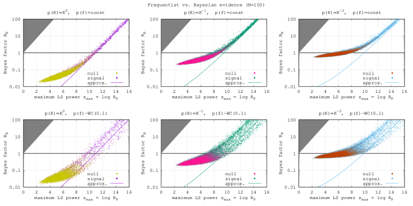
Figure 3: Relationship between the frequentist and Bayesian detection metrics $R_{\rm F}$ and $R_{\rm B}$, assuming $6$ different priors. Each point in a graph represents a single MC trial, with $10^{4}$ points for the model $\mathcal{M}_{1}$ (“null” label) and $10^{4}$ points for $\mathcal{M}_{2}$ (“signal”). We also show the approximation (19), and the general boundary $R_{\rm B}\leq R_{\rm F}$ that follows from (1,3). For the “signal” part, the population priors coincide with the ones assumed in $R_{\rm B}$. This plot is for $N=100$ even timings, and analogous plots for $N=10$ and $N=30$, as well as for $N=100$ random timings, are available in the online-only supplement.

First of all, let us verify the relationship (19) between the $R_{\rm F}$ and $R_{\rm B}$ metrics. These quantities are plotted against each other in Fig. 3, for all $6$ available priors (“objective” and “subjective” priors are identical here). Three cases with uniform-frequency priors (top row of plots) reveal good agreement with (19), at least for $z_{\max}\gtrsim 10$. Smaller $z_{\max}$ reveal a systematic deviation from (19), but some near-deterministic relationship clearly remains, because the random spread keeps small. This indicates that (19) needs a correction in the low-$z$ range, but nevertheless $R_{\rm F}$ and $R_{\rm B}$ remain tightly connected with each other over the entire range. They should then appear statistically equivalent in terms of their $\alpha\beta$ diagrams. This conclusion requires uniform $p_{f}$, and provided that holds for all $p_{K}$.

We can see significant changes to the picture when the frequency prior becomes nonuniform (bottom row of Fig. 3). Nearly-deterministic relationship between $R_{\rm F}$ and $R_{\rm B}$ turns into just a correlation, with a large spread covering about an order of magnitude. The formula (19) may still serve as an average prediction to the Bayes factor, but it can be several times larger or several times smaller than that. In this case we may possibly expect a statistical difference between these metrics that can be revealed using the $\alpha\beta$ diagram.

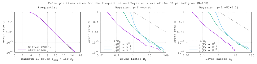
Figure 4: Simulated $\alpha$ curves for the frequentist and Bayesian detection metric, $R_{\rm F}$ and $R_{\rm B}$. While $R_{\rm F}$ does not depend on any prior and is shown as a single curve, the $R_{\rm B}$ curves are shown for $6$ priors. We also show an analytic ${\rm FAP}$ approximation from (Baluev, 2008) for $R_{\rm F}$, and the boundary (14) for $R_{\rm B}$. By definition, all curves shown here assume only the $\mathcal{M}_{1}$ model, so population priors do not get involved. This plot is for $N=100$ even timings, and analogous plots for $N=10$ and $N=30$, as well as for $N=100$ random timings, are available in the online-only supplement.

But before considering $\alpha\beta$ diagrams, let us investigate how well the Bayes factor is calibrated against false positives. Recall that there is a common empiric scale for $R_{\rm B}$ due to Jeffreys (1998) that should enable (in theory) its use without resorting to any mistakes rates. But simultaneously, such a scale can be constructed more objectively from the $\alpha(R_{\rm B})$ function, on a task-by-task basis. So let us see how well these two scales agree with each other in the LSP/BLSP framework.

Fig. 4 demonstrates several $\alpha$ curves for all $6$ priors (still assuming identical “subjective” and “objective” ones). Though the curves are rather different, one common tendency is an unexpectedly small $\alpha$ level for $R_{\rm B}=1$. This $R_{\rm B}$ level should indicate, based on the empiric scale, statistically equal models. But for $p_{K}=\mathop{\rm const}\nolimits$ the level $R_{\rm B}=1$ appears actually quite decisive in favour of $\mathcal{M}_{2}$, because it has $\alpha<0.01$. An inconclusive case should occur for $\alpha\sim 0.5$ that corresponds to $R_{\rm B}<0.1$ (for the same $p_{K}=\mathop{\rm const}\nolimits$). However, based on the empiric scale such $R_{\rm B}$ would indicate a strong support in favour of $\mathcal{M}_{1}$ over $\mathcal{M}_{2}$. Therefore, the empiric scale of $R_{\rm B}$ turns to be very overconservative compared to the ${\rm FAP}$ calibration.

Practical consequences of such a miscalibration are likely not that bad, if there is no mismatch between the “subjective” and “objective” prior. From further investigation of Fig. 4 we can see that overconservative behaviour of $R_{\rm B}$ is tied to $p_{K}$ and mainly appears if $p_{K}$ leans towards larger-amplitude signals. For example, for $p_{K}=\mathop{\rm const}\nolimits$ possible inaccuracy of the $R_{\rm B}$ threshold is unlikely to affect the number of detected signals very much because the population is mostly located at much larger amplitudes. Moreover, for large $R_{\rm B}$ the miscalibration effect gets reduced regardless of $p_{K}$, for example $R_{\rm B}\gtrsim 10$ imply more stable $\alpha$ values that are in a better agreement with the empiric scale.

Still the miscalibration effect is important if the “subjective” $p_{K}$ does not match the “objective” one. For example, we could wrongly assume $p_{K}=\mathop{\rm const}\nolimits$ (implying extremely conservative $R_{\rm B}$) while in actuality the objects are distributed as $p_{K}\propto K^{-1}$ or $p_{K}\propto K^{-2}$. In this case $R_{\rm B}$ that we actually use is systematically smaller than it would for the correct $p_{K}$. To make this worse, the $R_{\rm B}$ threshold is now located where the population is dense. Many detectable signals might then escape if we disregard the calibration against the ${\rm FAP}$. Notice that this miscalibration effect depends on $p_{K}$, but does not seem to depend (significantly) on $p_{f}$.

From now on, we assume that Bayes factor is always properly calibrated against the ${\rm FAP}$. Under that we mean that the function $\alpha(R_{\rm B})$ is used to treat whether the observed $R_{\rm B}$ is significant or not. So the results below do not include the miscalibration effect. This makes the analysis rather similar to the frequentist detection, however in the Bayesian case $\alpha(R_{\rm B})$ also depends on the adopted (subjective) prior. It is also possible to include the $\beta$ rate in such a calibration, if necessary, but this function depends on the subjective and objective priors both.

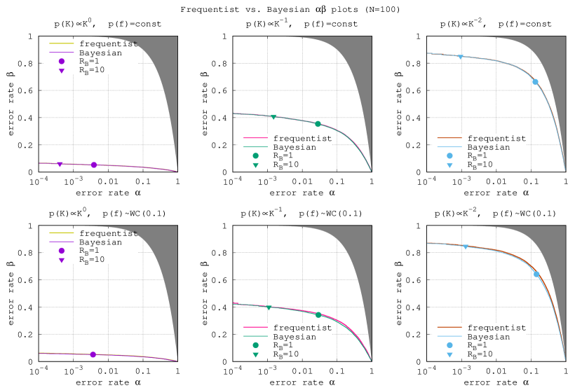
Figure 5: The $\alpha\beta$ diagrams intercomparing the frequentist and Bayesian detection metrics, for $6$ different priors, and for even timings with $N=100$. Each plot shows two simulated diagrams for $R_{\rm F}$ and $R_{\rm B}$ that always appear to nearly coincide. The positions of $R_{\rm B}=1$ and $R_{\rm B}=10$ are also shown for a reference (they depend on the prior). The population priors coincide with the ones used in $R_{\rm B}$. Analogous plots for all $36$ combinations of priors, including mismatch cases, and for all time series, are available in the online-only supplement.

Now let us proceed to our final goal, investigation of $\alpha\beta$ diagrams for the $R_{\rm F}$- and $R_{\rm B}$-based detection. In Fig. 5 they are shown for all $6$ cases when the “objective” and “subjective” priors match each other. In each diagram the frequentist and Bayesian curves nearly coincide, implying that these metrics are practically equivalent. Such a behaviour was expected for the case of uniform $p_{f}$, but for the nonuniform $p_{f}$ it surprisingly remains visually identical. Even though individual values of $R_{\rm B}$ have shown large spread because of nonconstant $p_{f}$, they generate nearly the same $\alpha\beta$ curve. Hence, there is no practical difference between Bayesian and frequentist period search, at least in model tasks we considered.

Entirely analogous picture appears for all $N$, and also in all cases with mismatched priors in all $36$ pairwise combinations (see online-only figures). It does not matter what the prior we select from our pool, Bayesian analysis always reveals practically the same $\alpha\beta$ diagram as the frequentist one. In terms of examples shown in Fig. 2, all our simulations were close to the third panel scheme.

Figure 6: Estimated efficiency differences $\delta I_{\alpha\beta}$ between Bayesian and frequentist signal detection, for all $36$ combinations of priors and $3$ even time series. Coordinates in each plot are integer indices enumerating the prior (same sequence as for plots in Fig. 3). Quarters that involve one or both nonuniform frequency priors are additionally highlighted by gray/darker-gray background. Blue points indicate advantage of Bayesian detection, while red ones indicate advantage of the frequentist one. The area of each point is proportional to $|\delta I_{\alpha\beta}|$, but untrustable points that have a greater-than-value uncertainty (significance below one-sigma) are shown empty. Points with uncertainty smaller than half of the value (significance above two-sigma) are additionally encircled.

To develop these findings further, we computed Monte Carlo estimates for all $I_{\alpha\beta}$, and the associated differences $\delta I_{\alpha\beta}$ between the $R_{\rm B}$- and $R_{\rm F}$-based detection. These differences are plotted in Fig. 6 for all $36$ combinations of priors. The values of $\delta I_{\alpha\beta}$ are demonstrated through sizes of points. Majority of values appeared consistent with zero (within the uncertainty). A sound (above two sigma) advantage of the Bayesian analysis over the frequentist one is revealed in just a few cases, whenever the adopted and actual prior involve nonuniform $p_{f}$. In half cases of mismatched priors (assuming nonuniform $p_{f}$ while the true one is uniform) we see an average advantage of the frequentist approach, though this looks a bit less reliable given the uncertainties. In case of an opposite mismatch (true $p_{f}$ is nonuniform but assuming it is uniform) our $\delta I_{\alpha\beta}$ looks mostly consistent with zero.

We hoped that the case of $N=10$ would reveal the biggest Bayesian/frequentist difference, because the role of the prior increases for smaller data, but in actuality this case revealed even smaller $\delta I_{\alpha\beta}$.

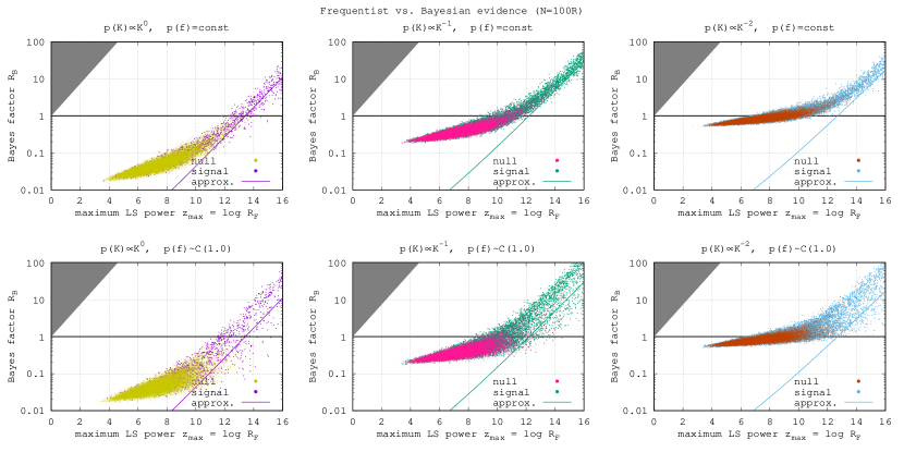
Figure 7: Same as Fig. 3, but for $N=100$ randomly spaced timings, and with frequency range increased by the factor of ten above $f_{\rm Ny}$.

Finally, we investigated the case of randomly spaced time series. We reiterate once more that the main reason for that was because random timings allow to consider much wider frequency range than the Nyquist one. In this test case we had $N=100$ and the maximum frequency ten times the previous limit $f_{\rm Ny}=\frac{1}{2}$. This corresponds to the factor $W$ in (16) about $\simeq 500$. Consequently, we have roughly $500$ peaks in a periodogram, so this is a rather large frequency range. In Fig. 7 we show the $R_{\rm F}$ vs. $R_{\rm B}$ diagram which appears generally similar to Fig. 3 and reveals similar relationships (nearly deterministic one for uniform $p_{f}$ and only correlational one for non-uniform $p_{f}$).

Figure 8: Same as plots of Fig. 6, but for $N=100$ randomly spaced timings, and with frequency range increased by the factor of ten above $f_{\rm Ny}$.

The simulated $\alpha\beta$ diagrams (see online supplement) again appear nearly identical for $R_{\rm F}$ and $R_{\rm B}$. The associated estimates of $\delta I_{\alpha\beta}$ are shown in Fig. 8, and they reveal only two cases above two-sigma. In general, these simulations appear quite similar to those for the even data.

In all the cases that we considered, absolute values of $\delta I_{\alpha\beta}$ remain below $0.02$, and usually below $0.01$. This is very formal and practically negligible difference, even if measurable. However, can this difference be boosted to a higher level, for example by tuning the nonuniform $p_{f}$ distribution?

First of all, it is necessary to derive, at least roughly, what characteristic of $p_{f}$ may define the $\alpha\beta$ curve. The frequentist test does not depend on $p_{f}$ at all, but Bayesian one does. This effect can be roughly assessed by intercomparing the Bayes factor approximations (18) and (19). We can obtain a relationship

$$\log R_{\rm B}\simeq\left.\log R_{\rm B}\right|_{p_{f}=\mathop{\rm const}\nolimits}+\log\left[f_{\rm u}\,p_{f}(f_{\max})\right],$$ (28)

where $f_{\max}$ being a random quantity, namely the frequency of the maximum periodogram peak. The distribution of $f_{\max}$ is not necessarily the same as $p_{f}$ and is also different for the null and alternative model. If $\mathcal{M}_{1}$ is true then there is no signal in the data and $f_{\max}$ is uniformly distributed in the range $[0,f_{\rm u}]$, since this is how noisy peaks are distributed in the LSP. If $\mathcal{M}_{2}$ is true, the maximum peak becomes correlated with the existing signal. In the ultimate case, when the signal amplitude is large, $f_{\max}$ becomes nearly certainly equal to the signal frequency. If the latter case was always true, the distribution of $f_{\max}$ should be the same as $p_{f}$, but in actuality it should be somewhere between the uniform one and the $p_{f}$. Still we can adopt $p_{f}$ as an ultimately nonuniform limit.

From (28) it follows that the first-order statistical effect imposed by the nonuniform $p_{f}$ is the bias of $\log R_{\rm B}$:

$$b=\mathbb{E}\left[\log R_{\rm B}-\left.\log R_{\rm B}\right|_{p_{f}=\mathop{\rm const}\nolimits}\right]\simeq\log f_{\rm u}+\mathbb{E}\log p_{f}(f_{\max}).$$ (29)

In case of model $\mathcal{M}_{1}$, this bias reads

$$b_{\rm I}\simeq\log f_{\rm u}+\frac{1}{f_{\rm u}}\int\limits_{0}^{f_{\rm u}}\log p_{f}(f_{\max})df_{\max},$$ (30)

and by setting $p_{f}$ to the Cauchy distribution (22) we obtain $b_{\rm I}\sim\mathop{\rm const}\nolimits-\log\frac{f_{\rm u}}{f_{0}}$ (this assumes $f_{\rm u}\gg f_{0}$). For the model $\mathcal{M}_{2}$, and assuming the $p_{f}$ distribution for $f_{\max}$, the bias can be expressed through the entropy $\mathcal{H}(p_{f})$:

$$b_{\rm II}\simeq\log f_{\rm u}+\int\limits_{0}^{f_{\rm u}}\log p_{f}(f_{\max})p_{f}(f_{\max})df_{\max}=\log f_{\rm u}-\mathcal{H}(p_{f}),$$ (31)

For the Cauchy distribution taken as $p_{f}$, we obtain $b_{\rm II}\sim\mathop{\rm const}\nolimits+\log\frac{f_{\rm u}}{f_{0}}$ (again for $f_{\rm u}\gg f_{0}$).

We can see that our primary quantity that determines statistical effect of $p_{f}$ is the ratio $\frac{f_{\rm u}}{f_{0}}$. This same quantity should likely define the first-order effect on the $\alpha\beta$ diagram. However, from (16) and (19) it follows that the dependency of $\alpha$ rate on $R_{\rm B}$ is roughly logarithmic, so the effect should be roughly proportional to $\log\frac{f_{\rm u}}{f_{0}}$. This logarithmic dependency explains why our simulations revealed so small difference between the frequentist and Bayesian $\alpha\beta$ diagrams: we had $\frac{f_{\rm u}}{f_{0}}=5$, and its logarithm is even a smaller number.

Now it appears not so easy to increase $\delta I_{\alpha\beta}$ by a remarkable amount. For example, to raise it above $\sim 0.1$ (still a modest level), we should increase $\log\frac{f_{\rm u}}{f_{0}}$ by an order of magnitude, and this scales to $\frac{f_{\rm u}}{f_{0}}\sim 10^{7}$. Such an extreme prior does not seem very realistic from the practical point of view. At least, we should have a sound physical basis justifying so nonuniform frequency distribution (to justify, for example, why we set tail p.d.f. levels to $\sim 10^{-14}$ instead of just zero). It seems that for a majority of practically reasonable frequency distributions $\delta I_{\alpha\beta}$ would likely remain about a few per cent, at most.

5 Discussion

Our main conclusion is that Bayesian and frequentist analyses reveal nearly equivalent efficiency in the task of sinusoidal signal detection. In case of the uniform frequency prior this follows explicitly from analytic approximations that express Bayes factor through the LSP. Cases involving nonuniform frequency prior reveal sometimes a formal advantage of Bayesian detection, but this may turn opposite whenever the adopted frequency prior does not match the actual distribution of periodic signals (and physical objects behind them). While the magnitude of Bayesian–frequentist difference $\delta I_{\alpha\beta}$ does depend on how much our frequency distribution is nonuniform, this dependence is shallow. It does not seem there is an easy way to achieve a large Bayesian advantage with a reasonable frequency prior.

Moreover, Bayes factor of this task may be rather poorly calibrated against the false alarm probability. For example, $R_{\rm B}=1$ may correspond to a situation of a clearly detectable signal (owing to low ${\rm FAP}$), rather than to a 50/50 case, as might be expected. In other words, Bayes factor may appear overconservative without the calibration. This effect depends of the signal’s amplitude prior, for example it is larger if this prior is biased towards relatively high-amplitude signals. However, the amplitude prior does not seem to affect detection efficiency much. The miscalibration effect becomes also more important in case of a mismatched prior.

Summarizing these results, Bayesian analysis does not appear very advantageous for the periodic signal detection, at least for the LSP models we were restricted to. In this task Bayes factor offers practically the same statistical efficiency as the frequentist periodogram, but requires more computing resources. Besides, additional issues appear because of miscalibration against the false positives rate.

In this work we considered only the basic formulation of the period search task within the Lomb model. More complicated cases may include (i) the use of a nontrivial null model, like linear or nonlinear trend, (ii) nonsinusoidal periodic signals, (iii) signals built from multiple components (like multiple sinusoids), (iv) dedicated noise models like Gaussian processes. Whenever the mathematical complexity (nonlinearity) of our models grows, the divergence between statistical metrics like $R_{\rm F}$ and $R_{\rm B}$ may grow as well. For example, in (Baluev, 2015b) it was demonstrated that hidden singularities of the likelihood function may significantly decrease the efficiency of the maximum-likelihood metric $E_{\rm F}$ and even to render it useless, because maxima are trapped by singularities. This is in fact an ultimate example of model nonlinearity. The issue can be solved by using a regularized model that eliminates singularities from the likelihood. However, Bayesian metric $E_{\rm B}$ may perform more or less well even without such a regularization, because it relies on integration, which is less sensitive to singularities. It is thereby interesting to perform a similar calibration of Bayesian analysis for such models, but this task is for a separate work.

Yet another issue that fell out of our scope is the issue of aliasing. While we considered uneven timings above, their only purpose was to increase the maximum frequency above the Nyquist one. But uneven data are usually considered in the context of aliases, that is regarding the task of distinguishing between nearly equivalent models that involve alternative periods. In our study possible aliases would be a nuisance factor, so we tried to suppress the aliasing by drawing uneven timings from the uniform distribution. However, aliasing comprises a separate challenge that can be solved either by the frequentist or Bayesian way, and systematic intercomparison of their efficiency is another topic for a future research.

Data availability

The data underlying this article are available in the article and in its online supplementary material.

Appendix A Deriving inequality for Bayesian prior predictive ${\rm FAP}$

Consider Bayesian ${\rm FAP}$ based on the prior predictive average:

$$\alpha_{\rm avg}(R_{\rm B}^{*}) = \int{\rm FAP}(R_{\rm B}^{*}|\mn@boldsymbol{\theta}_{1})\mathcal{W}_{1}(\mn@boldsymbol{\theta}_{1})d\mn@boldsymbol{\theta}_{1},$$

$${\rm FAP}(R_{\rm B}^{*}|\mn@boldsymbol{\theta}_{1}) = \int\limits_{E_{\rm B}(\mn@boldsymbol{x}|\mathcal{M}_{2},\mathcal{W}_{2})\geq\atop\phantom{\geq}R_{\rm B}^{*}E_{\rm B}(\mn@boldsymbol{x}|\mathcal{M}_{1},\mathcal{W}_{1})}L(\mn@boldsymbol{x}|\mn@boldsymbol{\theta}_{1},\mathcal{M}_{1})d\mn@boldsymbol{x}.$$ (32)

By substituting the second equation into the first one and interchanging integrals, we can simplify this to

$$\alpha_{\rm avg}(R_{\rm B}^{*})=\int\limits_{E_{\rm B}(\mn@boldsymbol{x}|\mathcal{M}_{2},\mathcal{W}_{2})\geq\atop\phantom{\geq}R_{\rm B}^{*}E_{\rm B}(\mn@boldsymbol{x}|\mathcal{M}_{1},\mathcal{W}_{1})}E_{\rm B}(\mn@boldsymbol{x}|\mathcal{M}_{1},\mathcal{W}_{1})\,d\mn@boldsymbol{x}.$$ (33)

The $\beta$ measure can be expressed in a similar way:

$$1-\beta_{\rm avg}(R_{\rm B}^{*})=\int\limits_{E_{\rm B}(\mn@boldsymbol{x}|\mathcal{M}_{2},\mathcal{W}_{2})\geq\atop\phantom{\geq}R_{\rm B}^{*}E_{\rm B}(\mn@boldsymbol{x}|\mathcal{M}_{1},\mathcal{W}_{1})}E_{\rm B}(\mn@boldsymbol{x}|\mathcal{M}_{2},\mathcal{W}_{2})\,d\mn@boldsymbol{x}.$$ (34)

We can see that the integration domains in (33) and (34) are determined identically. Moreover, the inequality that defines this domain applies to the integrands within this domain, hence to the integrals themselves. This results in the following inequality:

$$1-\beta_{\rm avg}(R_{\rm B}^{*})\geq R_{\rm B}^{*}\alpha_{\rm avg}(R_{\rm B}^{*}).$$ (35)

Then (14) follows immediately.

Appendix B The wrapped Cauchy distribution

The wrapped Cauchy (WC) distribution is obtained by applying the wrapping transform (21) to the p.d.f. (22). WC p.d.f. and c.d.f. are known and both can be expressed by simple analytic formulae (Mardia & Jupp, 1999, § 3.5.7). In our normalizations they look like

$$\mathrm{WC}(f_{0}):$$

$$p_{f}^{\rm obs}(f) = \frac{2\sinh(2\pi f_{0})}{\cosh(2\pi f_{0})-\cos(2\pi f)},$$

$$P_{f}^{\rm obs}(f) = \frac{1}{\pi}\arccos\frac{\cosh(2\pi f_{0})\cos(2\pi f)-1}{\cosh(2\pi f_{0})-\cos(2\pi f)},$$ (36)

$$f\in\left[0,f_{\rm Ny}=\frac{1}{2}\right].$$

A few sample plots of this functions are shown in Fig. 9.

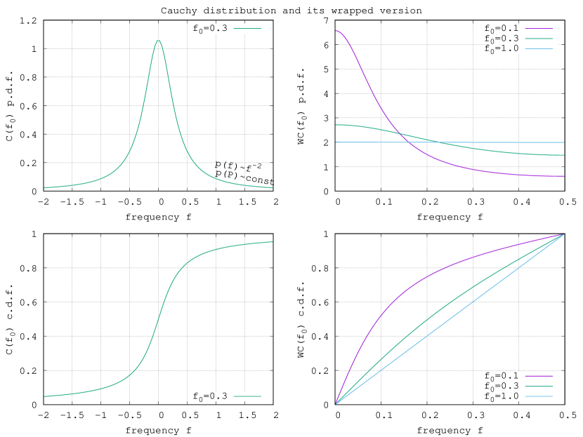
Figure 9: A few sample plots of the wrapped Cauchy distribution and of the corresponding Cauchy distribution it originates from. The Nyquist frequency is $f_{\rm Ny}=\frac{1}{2}$.

The function $P_{f}^{\rm obs}(f)$ is also easily invertible:

$$f=\frac{1}{2\pi}\arccos\frac{1+\cosh(2\pi f_{0})\cos(\pi P_{f}^{\rm obs})}{\cosh(2\pi f_{0})+\cos(\pi P_{f}^{\rm obs})}.$$ (37)

This enables a quick generation of random numbers from the WC distribution, by replacing $P_{f}^{\rm obs}$ in (37) with a standard uniform random variate.

Appendix C Computing the variance of $I_{\alpha\beta}$ estimate

First of all, from (24) we have

$$\mathbb{E}\hat{I}_{\alpha\beta}=\frac{1}{N_{\rm I}N_{\rm II}}\sum_{i=1}^{N_{\rm II}}\sum_{j=1}^{N_{\rm I}}\Pr(\tau_{j}^{\rm I}>\tau_{i}^{\rm II}),$$ (38)

because $\mathbb{E}H(*)$ has the meaning of probability. Now let us express the variance of (24) by taking its square, then applying the mathematical expectation operator, and subtracting the squared (38):

$$\mathbb{D}\hat{I}_{\alpha\beta} = \frac{1}{N_{\rm I}^{2}N_{\rm II}^{2}}\sum_{i=1}^{N_{\rm II}}\sum_{j=1}^{N_{\rm I}}\sum_{k=1}^{N_{\rm II}}\sum_{l=1}^{N_{\rm I}}\left\{\mathbb{E}\left[H(\tau_{j}^{\rm I}-\tau_{i}^{\rm II})H(\tau_{l}^{\rm I}-\tau_{k}^{\rm II})\right]-\right.$$ (39)

$$\left.-\Pr(\tau_{j}^{\rm I}>\tau_{i}^{\rm II})\Pr(\tau_{l}^{\rm I}>\tau_{k}^{\rm II})\right\}.$$

Now the behaviour of the common term $T=\mathbb{E}[H(*)H(*)]$ depends on whether the indices $(i,j,k,l)$ are all different or some of them coincide. There are four distinct cases:

1. $i=k$ and $j=l$ implies that $T=\mathbb{E}H^{2}(\tau_{j}^{\rm I}-\tau_{i}^{\rm II})=\Pr(\tau_{j}^{\rm I}>\tau_{i}^{\rm II})$;

2. $i=k$ but $j\neq l$ implies that $T=\mathbb{E}H[\min(\tau_{j}^{\rm I},\tau_{l}^{\rm I})-\tau_{i}^{\rm II}]=\Pr[\tau_{i}^{\rm II}<\min(\tau_{j}^{\rm I},\tau_{l}^{\rm I})]$;

3. $j=l$ but $i\neq k$ implies that $T=\mathbb{E}H[\tau_{j}^{\rm I}-\max(\tau_{i}^{\rm II},\tau_{k}^{\rm II})]=\Pr[\tau_{j}^{\rm I}>\max(\tau_{i}^{\rm II},\tau_{k}^{\rm II})]$;

4. $j\neq l$ and $i\neq k$ represents the most frequent case and implies that $T=\Pr(\tau_{j}^{\rm I}>\tau_{i}^{\rm II})\Pr(\tau_{l}^{\rm I}>\tau_{k}^{\rm II})$ that cancels with the identical product subtracted in (39).

Summing all this up, we have

$$\mathbb{D}\hat{I}_{\alpha\beta} = \frac{1}{N_{\rm I}^{2}N_{\rm II}^{2}}\sum_{i=1}^{N_{\rm II}}\sum_{j=1}^{N_{\rm I}}\left\{\Pr(\tau_{j}^{\rm I}>\tau_{i}^{\rm II})-\left[\Pr(\tau_{j}^{\rm I}>\tau_{i}^{\rm II})\right]^{2}\right\}+$$ (40)

$$+ \frac{1}{N_{\rm I}^{2}N_{\rm II}^{2}}\sum_{i=1}^{N_{\rm II}}\sum_{j=1}^{N_{\rm I}}\sum_{l=1\atop l\neq j}^{N_{\rm I}}\left\{\Pr[\tau_{i}^{\rm II}<\min(\tau_{j}^{\rm I},\tau_{l}^{\rm I})]-\right.$$

$$\left.-\Pr(\tau_{j}^{\rm I}>\tau_{i}^{\rm II})\Pr(\tau_{l}^{\rm I}>\tau_{i}^{\rm II})\right\}+$$

$$+ \frac{1}{N_{\rm I}^{2}N_{\rm II}^{2}}\sum_{i=1}^{N_{\rm II}}\sum_{j=1}^{N_{\rm I}}\sum_{k=1\atop k\neq i}^{N_{\rm II}}\left\{\Pr[\tau_{j}^{\rm I}>\max(\tau_{i}^{\rm II},\tau_{k}^{\rm II})]-\right.$$

$$\left.-\Pr(\tau_{j}^{\rm I}>\tau_{i}^{\rm II})\Pr(\tau_{j}^{\rm I}>\tau_{k}^{\rm II})\right\}.$$

Now, let us use two identities $\Pr(\tau^{\rm I}>t)=\mathbb{E}\alpha(t)$ and $\Pr(\tau^{\rm II}<t)=\mathbb{E}\beta(t)$ to transform (40) as follows:

$$\mathbb{D}\hat{I}_{\alpha\beta} = \frac{1}{N_{\rm I}^{2}N_{\rm II}^{2}}\sum_{i=1}^{N_{\rm II}}\sum_{j=1}^{N_{\rm I}}\left\{\mathbb{E}\beta(\tau_{j}^{\rm I})-\left[\mathbb{E}\beta(\tau_{j}^{\rm I})\right]^{2}\right\}+$$ (41)

$$+ \frac{1}{N_{\rm I}^{2}N_{\rm II}^{2}}\sum_{i=1}^{N_{\rm II}}\sum_{j=1}^{N_{\rm I}}\sum_{l=1\atop l\neq j}^{N_{\rm I}}\left\{\mathbb{E}\beta[\min(\tau_{j}^{\rm I},\tau_{l}^{\rm I})]-\right.$$

$$\left.-\mathbb{E}\beta(\tau_{j}^{\rm I})\mathbb{E}\beta(\tau_{l}^{\rm I})\right\}+$$

$$+ \frac{1}{N_{\rm I}^{2}N_{\rm II}^{2}}\sum_{i=1}^{N_{\rm II}}\sum_{j=1}^{N_{\rm I}}\sum_{k=1\atop k\neq i}^{N_{\rm II}}\left\{\mathbb{E}\alpha[\max(\tau_{i}^{\rm II},\tau_{k}^{\rm II})]-\right.$$

$$\left.-\mathbb{E}\alpha(\tau_{i}^{\rm II})\mathbb{E}\alpha(\tau_{k}^{\rm II})\right\}.$$

Here $\mathbb{E}\alpha(\tau^{\rm II})=\mathbb{E}\beta(\tau^{\rm I})=I_{\alpha\beta}$ by definition (8). Also, because $\alpha,\beta$ are monotonic we can replace $\alpha[\min(x,y)]=\max[\alpha(x),\alpha(y)]$ and $\beta[\min(x,y)]=\min[\beta(x),\beta(y)]$:

$$\mathbb{D}\hat{I}_{\alpha\beta} = \frac{1}{N_{\rm I}^{2}N_{\rm II}^{2}}\sum_{i=1}^{N_{\rm II}}\sum_{j=1}^{N_{\rm I}}\left(I_{\alpha\beta}-I_{\alpha\beta}^{2}\right)+$$ (42)

$$+ \frac{1}{N_{\rm I}^{2}N_{\rm II}^{2}}\sum_{i=1}^{N_{\rm II}}\sum_{j=1}^{N_{\rm I}}\sum_{l=1\atop l\neq j}^{N_{\rm I}}\left\{\mathbb{E}\min[\beta(\tau_{j}^{\rm I}),\beta(\tau_{l}^{\rm I})]-I_{\alpha\beta}^{2}\right\}+$$

$$+ \frac{1}{N_{\rm I}^{2}N_{\rm II}^{2}}\sum_{i=1}^{N_{\rm II}}\sum_{j=1}^{N_{\rm I}}\sum_{k=1\atop k\neq i}^{N_{\rm II}}\left\{\mathbb{E}\min[\alpha(\tau_{i}^{\rm II}),\alpha(\tau_{k}^{\rm II})]-I_{\alpha\beta}^{2}\right\}.$$

Now let us deal with, for example, the following term:

$$\mathbb{E}\min[\beta(\tau_{j}^{\rm I}),\beta(\tau_{l}^{\rm I})]=\int\limits_{0}^{1}\int\limits_{0}^{1}\min(\beta_{j},\beta_{l})d\alpha_{j}d\alpha_{l}=$$

$$=\int\limits_{0}^{1}d\alpha_{j}\left[\int\limits_{0}^{\alpha_{j}}\min(\beta_{j},\beta_{l})d\alpha_{l}+\int\limits_{\alpha_{j}}^{1}\min(\beta_{j},\beta_{l})d\alpha_{l}\right].$$ (43)

Since two inner integrals have such limits that either $\alpha_{l}<\alpha_{j}$ or $\alpha_{l}>\alpha_{j}$, this implies that $\beta_{l}>\beta_{j}$ or $\beta_{l}<\beta_{j}$ inside them, respectively. Therefore, the minima can be replaced with either $\beta_{j}$ or $\beta_{l}$, and

$$\mathbb{E}\min[\beta(\tau_{j}^{\rm I}),\beta(\tau_{l}^{\rm I})]=\int\limits_{0}^{1}d\alpha_{j}\left[\int\limits_{0}^{\alpha_{j}}\beta_{j}d\alpha_{l}+\int\limits_{\alpha_{j}}^{1}\beta_{l}d\alpha_{l}\right]=$$

$$=\int\limits_{0}^{1}\beta_{j}d\alpha_{j}\int\limits_{0}^{\alpha_{j}}d\alpha_{l}+\int\limits_{0}^{1}d\alpha_{j}\int\limits_{\alpha_{j}}^{1}\beta_{l}d\alpha_{l}=$$

$$=\int\limits_{0}^{1}\alpha_{j}\beta_{j}d\alpha_{j}+\int\limits_{0}^{1}d\alpha_{l}\int\limits_{0}^{\alpha_{l}}\beta_{l}d\alpha_{j}=2\int\limits_{0}^{1}\alpha\beta d\alpha=\int\limits_{0}^{1}\alpha^{2}d\beta.$$ (44)

The term with $\min[\alpha(\tau_{i}^{\rm II}),\alpha(\tau_{k}^{\rm II})]$ can be expressed by analogy and (42) finally turns into

$$\mathbb{D}\hat{I}_{\alpha\beta} = \frac{I_{\alpha\beta}-I_{\alpha\beta}^{2}}{N_{\rm I}N_{\rm II}}+$$ (45)

$$+ \frac{N_{\rm I}-1}{N_{\rm I}N_{\rm II}}\left(\int\limits_{0}^{1}\alpha^{2}d\beta-I_{\alpha\beta}^{2}\right)+$$

$$+ \frac{N_{\rm II}-1}{N_{\rm I}N_{\rm II}}\left(\int\limits_{0}^{1}\beta^{2}d\alpha-I_{\alpha\beta}^{2}\right).$$

By neglecting small terms we obtain (25).

Appendix D Online-only material

An archive with a complete set of figures in scaleable EPS format. The detailed description of each figure is given in the Readme file inside the archive.

References

- Baluev (2008) Baluev R. V., 2008, MNRAS, 385, 1279
- Baluev (2009a) Baluev R. V., 2009a, MNRAS, 393, 969
- Baluev (2009b) Baluev R. V., 2009b, MNRAS, 395, 1541
- Baluev (2012) Baluev R. V., 2012, MNRAS, 422, 2372
- Baluev (2013a) Baluev R. V., 2013a, MNRAS, 429, 2052
- Baluev (2013b) Baluev R. V., 2013b, MNRAS, 436, 807
- Baluev (2014) Baluev R. V., 2014, Astrophysics, 57, 434
- Baluev (2015a) Baluev R. V., 2015a, MNRAS, 446, 1478
- Baluev (2015b) Baluev R. V., 2015b, MNRAS, 446, 1493
- Bayarri & Berger (2000) Bayarri M. J., Berger J. O., 2000, Journal of the American Statistical Association, 95, 1127
- Bayarri & Berger (2013) Bayarri M. J., Berger J. O., 2013, in Damien et al. (2013), Chapt. 18, pp 361–394, Chapt. 18, pp 361–394
- Box (1980) Box G. E. P., 1980, J. Roy. Stat. Soc. A, 143, 383
- Bretthorst (2001a) Bretthorst G. L., 2001a, AIP Conf. Proc., 568, 241
- Bretthorst (2001b) Bretthorst G. L., 2001b, AIP Conf. Proc., 568, 246
- Brewer & Foreman-Mackey (2016) Brewer B. J., Foreman-Mackey D., 2016, arxiv.org:1606.03757
- Cumming (2004) Cumming A., 2004, MNRAS, 354, 1165
- Cumming et al. (1999) Cumming A., Marcy G. W., Butler R. P., 1999, ApJ, 526, 890
- Damien et al. (2013) Damien P., Dellaportas P., Polson N. G., Stephens D. A., eds, 2013, Bayesian Theory and Applications. Oxford University Press, Oxford
- Dawson & Fabrycky (2010) Dawson R. I., Fabrycky D. C., 2010, ApJ, 722, 937
- Draper (2013) Draper D., 2013, in Damien et al. (2013), Chapt. 20, pp 409–431, Chapt. 20, pp 409–431
- Feroz et al. (2009) Feroz F., Hobson M. P., Bridges M., 2009, MNRAS, 398, 1601
- Ferraz-Mello (1981) Ferraz-Mello S., 1981, AJ, 86, 619
- Gelman (2008) Gelman A., 2008, Bayesian Analysis, 3, 445
- Hara et al. (2017) Hara N. C., Boué G., Laskar J., Correia A. C. M., 2017, MNRAS, 464, 1220
- Jeffreys (1998) Jeffreys S. H., 1998, Theory of Probability (The International series of monographs on physics) 3rd Edition. Oxford University Press
- Koroluk et al. (1985) Koroluk V. S., Portenko N. I., Skorokhod A. V., Turbin A. F., 1985, A handbook on the probability theory and mathematical statistics (in Russian). Naukova dumka, Kyev
- Lomb (1976) Lomb N. R., 1976, Ap&SS, 39, 447
- Mardia & Jupp (1999) Mardia K. V., Jupp P. E., 1999, Directional Statistics. John Wiley & Sons Ltd
- Mortier et al. (2014) Mortier A., Faria J. P., Correia C. M., Santerne A., Santos N. C., 2014, A&A, 573, A101
- Nelson et al. (2020) Nelson B. E., et al., 2020, AJ, 159, 73
- Scargle (1982) Scargle J. D., 1982, ApJ, 263, 835
- Schuster (1898) Schuster A., 1898, Terrestial Magnetism and Atmospheric Electricity, 3, 13
- Schwarzenberg-Czerny (1998) Schwarzenberg-Czerny A., 1998, Baltic Astron., 7, 43
- Skilling (2004) Skilling J., 2004, AIP Conf. Proc., 735, 395
- Vaníček (1969) Vaníček P., 1969, Ap&SS, 4, 387
- Weinberg (2012) Weinberg M. D., 2012, Bayesian Analysis, 7, 737
- Zechmeister & Kürster (2009) Zechmeister M., Kürster M., 2009, A&A, 496, 577