Analysis of Fully Discrete Mixed Finite Element Scheme for Stochastic Navier-Stokes Equations with Multiplicative Noise

Abstract

This paper is concerned with stochastic incompressible Navier-Stokes equations with multiplicative noise in two dimensions with respect to periodic boundary conditions. Based on the Helmholtz decomposition of the multiplicative noise, semi-discrete and fully discrete time-stepping algorithms are proposed. The convergence rates for mixed finite element methods based time-space approximation with respect to convergence in probability for the velocity and the pressure are obtained. Furthermore, with establishing some stability and using the negative norm technique, the partial expectations of the $H^{1}$ and $L^{2}$ norms of the velocity error are proved to converge optimally.

1 Introduction

In this paper, we consider the following time-dependent stochastic incompressible Navier-Stokes equations:

(1a) $$du =\bigl{[}\nu\Delta u-(u\cdot\nabla)u-\nabla p\bigr{]}dt+G(u)dW \qquad\mbox{a.s. in}\,D_{T}:=(0,T)\times D,$$

(1b) $$\mbox{\rm div\,}u =0 \qquad\mbox{a.s. in}\,D_{T},$$

(1c) $$u(0) =u_{0} \qquad\mbox{a.s. in}\,D,$$

where $T>0$ denotes time, $\nu>0$ is the viscosity of the fluid, ${u}$ and $p$ denote respectively the velocity and the pressure of the problem (1) which are spatially periodic with period $L>0$, and $D=(0,L)^{2}\subset\mathbb{R}^{2}$ is a period of the periodic domain with boundary $\partial D$ and $u_{0}$ denotes a given initial datum. Here we assume that $\{W(t);t\geq 0\}$ is an $[L^{2}(D)]^{2}$-valued $Q$-Wiener process. The noise is not divergence-free (i.e., $\mbox{\rm div\,}G(u)\neq 0$).

The stochastic system (1) can take into account noise term in the sense of physical or numerical uncertainties and thermodynamical fluctuations. In [2], Bensoussan and Temam started to study the stochastic Navier-Stokes in mathematical investigation. The paper [16] by Flandoli and Gatarek developed a fully stochastic theory to prove the existence of a martingale solution. This paper [20] investigated the ergodic properties for the stochastic Navier-Stokes equations with degenerate noise. In the last twenty years, there is a large amount of literature about the analysis of problem (1). We refer to [1, 19, 3, 4, 10, 12, 14, 15] and the references therein for detailed discussions of the stochastic incompressible Navier-Stokes equations.

The paper [7] by Brzeźniak, et al. proposed two fully discrete finite element schemes for the stochastic Navier-Stokes equations with multiplicative noise. By using the compactness argument, the authors analyzed the convergence for the velocity field to weak martingale solutions in 3D and to strong solutions in 2D. In [10], Carelli and Prohl studied implicit and semi-implicit fully schemes for the stochastic Navier-Stokes problem. The result in [10] is convergence of rate (amost) $\frac{1}{4}$ in time and linear convergence in space for the velocity. However, the convergence of the pressure was not given. In work [3], the authors proposed an iterative splitting scheme for stochastic Navier-Stokes equations and established a strong convergence in probability in the 2D case. In [4], the authors studied another time-stepping semi-discrete scheme and derived strong $L^{2}$ convergence for the velocity. In [17], Hausenblas and Randrianasolo proposed a time semi-discrete scheme of stochastic 2D Navier-Stokes equations with penalty-projection method. As noted in [17], the result is convergence of rate (amost) $\frac{1}{4}$ in time for the velocity and the pressure. In paper [14], Feng and Qiu developed a fully discrete mixed finite element scheme of the time-dependent stochastic Stokes equations with multiplicative noise and established strong convergence with rates not only for the velocity but also for the pressure. The paper [15], by Feng, et al. proposed a new fully discrete mixed finite element scheme of the time-dependent stochastic Stokes equations with multiplicative noise and obtained optimal strong convergence with rates for both the velocity and the pressure. In a very recent paper [5], Breit and Dodgson considered a fully discrete time-space finite element scheme and proved strong convergence with rates for the velocity. The result in [5] is convergence of rate (amost) $\frac{1}{2}$ in time and linear convergence in space. The error estimate of the velocity field $u$ and its time-space numerical solution $u_{h}^{n}$ reads as: assume that $Lk\leq(-\epsilon\log h)^{-1}$ for some $L>0$, then for any $\alpha<\frac{1}{2}$

(2) $$\mathbb{E}\Bigl{[}\Omega_{k,h}^{\epsilon}\Bigl{(}\max_{1\leq n\leq N}\|u(t_{n})-u^{n}_{h}\|^{2}_{L^{2}_{x}} +k\sum_{n=1}^{N}\|\nabla(u(t_{n})-u^{n}_{h})\|^{2}_{L^{2}_{x}}\Bigr{)}\Bigr{]}$$

$$\leq C\bigl{(}k^{2\alpha-\epsilon}+h^{2}\bigr{)},$$

where $\Omega_{k,h}^{\epsilon}\subset\Omega$ with $\mathbb{P}(\Omega\backslash\Omega_{k,h}^{\epsilon})\rightarrow 0$ as $k,h\rightarrow 0$.

The primary goal of this paper is twofold. Our first goal is to develop an optimally convergent fully discrete finite element scheme with inf-sup stability. Our main idea, which is partly used in references [14, 15], is to use the Helmholtz decomposition for the driving multiplicative noise at each time step, and then solve velocity and pressure. We propose new semi-discrete and fully discrete time-stepping algorithms for problem (1) and prove the convergence of the velocity and the pressure for the fully discrete scheme for the stochastic Navier-Stokes equations. The second goal is to prove strong optimal $H^{1}$ convergence first, and then to obtain $L^{2}$ convergence of the fully discrete scheme with the negative norm technique. To the best of our knowledge, it is the first time that strong optimal $L_{t}^{\infty}-H_{x}^{1}/L_{x}^{2}$ convergence of the discrete solution $(u_{h}^{n},p_{h}^{n})$ to a fully discrete system of the stochastic Navier-Stokes equations has been established. The highlight of this paper (see section 4) is to derive the error estimates for the numerical solution as follows: for any $\alpha<\frac{1}{2}$

(3) $$\mathbb{E}\Bigl{[}\textbf{1}_{\Omega_{k,h}^{\epsilon}\cap\Omega_{h,h}^{\epsilon}\cap\Omega_{h}^{\epsilon}\cap\Omega_{\tau}^{\epsilon}}\Bigl{(}\|\nabla(u(t_{n})-u^{n}_{h})\|^{2}_{L^{2}_{x}}\Bigr{)}\Bigr{]} \leq C\bigl{(}k^{2\alpha-\epsilon}+h^{2-4\epsilon}\bigr{)},$$

(4) $$\mathbb{E}\Bigl{[}\textbf{1}_{\Omega_{k}^{\epsilon}\cap\Omega_{h}^{\epsilon}}\Bigl{(}\Bigl{\|}\int_{0}^{t_{m}}p(s)\,ds-k\sum^{m}_{n=1}p^{n}_{h}\Bigr{\|}^{2}_{L^{2}_{x}}\Bigr{)}\Bigr{]} \leq C\bigl{(}k^{2\alpha-\epsilon}+h^{2-2\epsilon}\bigr{)},$$

(5) $$\mathbb{E}\Bigl{[}\textbf{1}_{\Omega_{k,h}^{\epsilon}\cap\Omega_{h,h}^{\epsilon}\cap\Omega_{h}^{\epsilon}\cap\Omega_{k}^{\epsilon}\cap\Omega_{\kappa_{0}}\cap\Omega_{\kappa}}\Bigl{(}\|u(t_{n})-u^{n}_{h}\|^{2}_{L^{2}_{x}}\Bigr{)}\Bigr{]} \leq C(\kappa_{0},\kappa_{1})\bigl{(}k^{2\alpha-4\epsilon}+h^{4-8\epsilon}\bigr{)}.$$

The remainder of this paper is organized as follows. In Section 2, we introduce some function and space notation for problem (1) and obtain a few preliminary results. In Section 3, we propose the semi-discrete scheme for problem (1) and derive some optimal error estimates for both the velocity and pressure approximations. In Section 4, we prove some optimal error estimates for the fully discrete scheme for problem (1) with the negative norm technique. In Section 5, some numerical results are given to validate the theoretical error estimates.

2 Preliminaries

2.1 Notation and assumptions

Standard function and space notation will be adopted in this paper. Let $H^{m}(D)$ $(m\geq 0)$ denote the standard Sobolev space, and $\|\cdot\|_{H^{m}_{x}}$ denotes its norm. Let $H^{m}_{per}(D)$ be the subspace of $H^{m}(D)$ consisting of $\mathbb{R}^{2}$-valued periodic function. Let $(\cdot,\cdot):=(\cdot,\cdot)_{D}$ denote the standard $L^{2}$-inner product. We also let $(\Omega,\mathfrak{F},\mathfrak{F}_{t},\mathbb{P})$ be a stochastic basis with a complete right continuous filtration. For a given random variable $v$ defined on $(\Omega,\mathfrak{F},\mathfrak{F}_{t},\mathbb{P})$, let $\mathbb{E}[v]$ denote the expected value of $v$. Let $X$ denote a normed vector space $X$ with norm $\|\cdot\|_{X}$. Define the following Bochner space

$$L^{p}(\Omega,X):=\bigl{\{}v:\Omega\rightarrow X;\,\mathbb{E}[\|v\|_{X}^{p}]<\infty\bigr{\}}$$

and the norm

$$\|v\|_{L^{p}(\Omega,X)}:=\Bigl{(}\mathbb{E}\Bigl{[}\|v\|_{X}^{p}\Bigr{]}\Bigr{)}^{\frac{1}{p}},\qquad 1<p<\infty.$$

We also define some special space notation as follows:

$$\mathcal{V}:=[H^{1}_{per}(D)]^{2},\quad\mathcal{W}:=\{q\in L^{2}_{per}(D);\,(q,1)_{D}=0\},\quad\mathcal{V}_{0}:=\bigl{\{}v\in\mathcal{V};\,\mbox{\rm div\,}v=0\mbox{ in }D\bigr{\}}.$$

Let $\mathcal{K}:=L_{0}(L_{per}^{2}(D);[L_{per}^{2}(D)]^{2})$ denote the Banach space of linear operators from $L_{per}^{2}(D)$ to $[L_{per}^{2}(D)]^{2}$ with finite Hilbert-Schmidt norms denoted by $\|\cdot\|_{\mathcal{K}}$. As it is noted [22] that the stochastic integral $\int_{0}^{t}\varphi(s)dW(s)$ is an $\{\mathfrak{F}_{t}\}$-martingale and the following Itô’s isometry holds:

(6) $$\mathbb{E}\Bigl{[}\Bigl{\|}\int_{0}^{T}\varphi(s)\,dW(s)\Bigr{\|}_{L^{2}_{x}}^{2}\Bigr{]}=\mathbb{E}\Bigl{[}\int_{0}^{T}\|\varphi(s)\|^{2}_{\mathcal{K}}\,ds\Bigr{]}.$$

In this paper we assume that $G:[0,T]\times[L_{per}^{2}(D)]^{2}\rightarrow L^{2}(\Omega,\mathcal{K})$ satisfies the following conditions:

(7a) $$\|G(v)-G(w)\|_{L_{2}(\mathcal{K},L^{2}_{x})} \leq C\|v-w\|_{L^{2}_{x}},\ \forall v,w\in[L_{per}^{2}(D)]^{2},$$

(7b) $$\|G(v)\|_{L_{2}(\mathcal{K},H^{i}_{x})} \leq C\bigl{(}1+\|v\|_{H^{i}_{x}}\bigr{)},\ \forall v\in[H_{per}^{i}(D)]^{2},\,i=1,2,$$

(7c) $$\|D^{j}G(v)\|_{L_{2}(\mathcal{K},\mathcal{L}([L^{2}(D)]^{j};L^{2}(D))} \leq C,\ \forall v\in[L_{per}^{2}(D)]^{2},\,j=1,2.$$

We introduce the Helmholtz projection [18] $P_{H}:[L_{per}^{2}(D)]^{2}\rightarrow\mathcal{V}$ defined by $P_{H}v=\eta$ for every $v\in[L_{per}^{2}(D)]^{2}$, where $(\eta,\xi)\in\mathcal{V}\times[H_{per}^{1}(D]^{2})/\mathbb{R}$ is a unique decomposition such that

$$v=\eta+\nabla\xi,$$

and $\xi\in[H_{per}^{1}(D)]^{2}/\mathbb{R}$ satisfies the following problem:

(8) $$(\nabla\xi,\nabla q)=(v,\nabla q),\qquad\forall q\in\mathcal{V}.$$

2.2 Definition of weak solutions

In this subsection we first recall the weak solution definition for problem (1), and refer to [9, 8, 14, 15]. We then introduce some regularity of the velocity and the pressure.

Definition 1.

Assume that $(\Omega,\mathfrak{F},(\mathfrak{F}_{t})_{t\geq 0},\mathbb{P})$ is a given stochastic basis and $u_{0}$ is an $\mathfrak{F}_{0}$-measurable random variable. Then $(u,p)$ is called a weak pathwise solution to problem (1) if

(i) the velocity and the pressure $(u,p)$ is $\mathfrak{F}_{t}$-adapted and

$$u\in C([0,T];[L_{per}^{2}(D)]^{2})\cap L^{2}([0,T;\mathcal{V}]), \quad\mathbb{P}\mbox{-a.s.},$$

$$p\in W^{-1,\infty}(0,T;\mathcal{W}), \quad\mathbb{P}\mbox{-a.s.}.$$

(ii) the problem (1) satisfies

(9a) $$\bigl{(}u(t),v\bigr{)} +\int_{0}^{t}\bigl{[}a(u(s),v)+b(u(s),u(s),v)\bigr{]}\,ds-d\Bigl{(}v,\int_{0}^{t}p(s)\,ds\Bigr{)}$$

$$=(u_{0},v)+\Bigl{(}\int_{0}^{t}G(u(s))\,dW(s),v\Bigr{)}\quad\forall\,v\in\mathcal{V},$$

(9b) $$d(u,q) =0,\quad\forall\,q\in\mathcal{W},$$

holds $\mathbb{P}$-a.s. for all $t\in(0,T]$. Where the bilinear forms $a(\cdot,\cdot)$ and $d(\cdot,\cdot)$ are defined

$$a(v,w) :=\nu\bigl{(}\nabla v,\nabla w\bigr{)}, \ \forall\,v,w\in\mathcal{V},$$

$$d(v,q) :=\bigl{(}\nabla\cdot v,q\bigr{)}, \ \forall\,v\in\mathcal{V},\,q\in\mathcal{W},$$

and the nonlinear form $b(\cdot,\cdot,\cdot)$ is defined as follows:

$$b(w,u,v) :=\bigr{(}w\cdot\nabla u,v\bigr{)}+\frac{1}{2}\bigr{(}(\nabla\cdot w)u,v\bigr{)},\ \forall\,w,u,v\in\mathcal{V}.$$

Using the similar idea in [15], problem (9) can be considered as a mixed formulation for problem (1). Thus, we introduce a new pressure $r:=p-\xi(u)\,dW$, where we apply the Helmholtz decomposition $G(u)=\eta(u)+\nabla\xi(u)$, where $\xi(u)\in\mathcal{V}$, $\mathbb{P}$-a.s. such that

$$(\nabla\xi(u),\nabla\phi)=(G(u),\nabla\phi),\qquad\forall\,\phi\in\mathcal{V}.$$

By the elliptic regularity [18], we have

(10) $$\|\nabla\xi(u)\|_{L^{2}_{x}} \leq C\|G(u)\|_{L^{2}_{x}},$$

(11) $$\|\nabla\xi(u)\|_{H^{2}_{x}/\mathbb{R}} \leq C\|\nabla\cdot G(u)\|_{L^{2}_{x}}.$$

Definition 2.

Assume that $(\Omega,\mathfrak{F},(\mathfrak{F}_{t})_{t\geq 0},\mathbb{P})$ is a given stochastic basis and $u_{0}$ is an $\mathfrak{F}_{0}$-measurable random variable. Then $(u,p)$ is called a weak pathwise solution to problem (1) if

(i) the velocity and the pressure $(u,r)$ is $\mathfrak{F}_{t}$-adapted and

$$u\in C([0,T];L_{per}^{2}(D))\cap L^{2}([0,T;\mathcal{V}]), \quad\mathbb{P}\mbox{-a.s.},$$

$$r\in W^{-1,\infty}(0,T;\mathcal{W}), \quad\mathbb{P}\mbox{-a.s.}.$$

(ii) the problem (1) satisfies

(12a) $$\bigl{(}u(t),v\bigr{)} +\int_{0}^{t}\bigl{[}a(u(s),v)+b(u(s),u(s),v)\bigr{]}\,ds-d\Bigl{(}v,\int_{0}^{t}r(s)\,ds\Bigr{)}$$

$$=(u_{0},v)+\Bigl{(}\int_{0}^{t}\eta(u(s))\,dW(s),v\Bigr{)}\quad\forall v\in\mathcal{V},$$

(12b) $$d(u,q) =0,\quad\forall q\in\mathcal{W},$$

holds $\mathbb{P}$-a.s. for all $t\in(0,T]$, where $\eta(u(s)):=G(u(s))-\nabla\xi(u(s))$.

Remark 1.

By using similar techniques in [19, 15], we note that $\int^{t}_{0}pds,\int^{t}_{0}rds\in L^{2}(\Omega,$ $L^{2}(0,T,\mathcal{W}))$.

The next Lemma follows from [5].

Lemma 3.

(i), Let $u_{0}\in L^{l}(\Omega,[L^{2}_{div}(D)]^{2})$ for some $l\geq 2$ and let $G$ satisfy (7). Then there exists a constant $C>0$, such that

$$\mathbb{E}\Bigl{[}\sup_{0\leq t\leq T}\|u(t)\|^{2}_{L^{2}_{x}} +\int_{0}^{T}\|\nabla u(s)\|_{L^{2}_{x}}^{2}ds\Bigr{]}^{\frac{l}{2}}\leq C.$$

(ii), Let $u_{0}\in L^{l}(\Omega,\mathcal{V}_{0})$ for some $l\geq 2$ and let $G$ satisfy (7). Then there exists a constant $C>0$, such that

$$\mathbb{E}\Bigl{[}\sup_{0\leq t\leq T}\|\nabla u(t)\|^{2}_{L_{x}^{2}}+\int_{0}^{T}\|\nabla^{2}u(s)\|_{L^{2}_{x}}^{2}ds\Bigr{]}^{\frac{l}{2}}\leq C.$$

(iii), Let $u_{0}\in L^{l}(\Omega,[H^{2}(D)]^{2}\cap\mathcal{V}_{0})\cap L^{5l}(\Omega,\mathcal{V}_{0})$ for some $l\geq 2$ and let $G$ satisfy (7). Then there exists a constant $C>0$, such that

$$\mathbb{E}\Bigl{[}\sup_{0\leq t\leq T}\|\nabla^{2}u(t)\|^{2}_{L_{x}^{2}}+\int_{0}^{T}\|\nabla^{3}u(s)\|_{L^{2}_{x}}^{2}ds\Bigr{]}^{\frac{l}{2}}\leq C.$$

We finish this section by establishing some regularity of pressure of various spatial norms. For the reader’s convenience, we here give theirs proofs.

Lemma 4.

(i), Let $u_{0}\in L^{l}(\Omega,L^{2}(D))$ for some $l\geq 2$ and let $G$ satisfy (7). Then there exists a constant $C>0$, such that

(13) $$\mathbb{E}\Bigl{[}\Bigl{\|}\int_{0}^{t}p(s)ds\Bigl{\|}^{2}_{L^{2}_{x}}\Bigl{]}^{\frac{l}{2}} \leq C,$$

(14) $$\mathbb{E}\Bigl{[}\Bigl{\|}\int_{0}^{t}\nabla p(s)ds\Bigl{\|}^{2}_{L^{2}_{x}}\Bigl{]}^{\frac{l}{2}} \leq C.$$

where $(u,p)$ is the weak pathwise solution to (1), cf. Definition 1.

(ii), Let $u_{0}\in L^{l}(\Omega,L^{2}(D))$ for some $l\geq 2$ and let $G$ satisfy (7). Then there exists a constant $C>0$, such that

(15) $$\mathbb{E}\Bigl{[}\Bigl{\|}\int_{0}^{t}r(s)ds\Bigl{\|}^{2}_{L^{2}_{x}}\Bigl{]}^{\frac{l}{2}} \leq C,$$

(16) $$\mathbb{E}\Bigl{[}\Bigl{\|}\int_{0}^{t}\nabla r(s)ds\Bigl{\|}^{2}_{L^{2}_{x}}\Bigl{]}^{\frac{l}{2}} \leq C.$$

where $(u,r)$ is the weak pathwise solution to (1), cf. Definition 2.

Proof.

For (13), from (9a), we have

(17) $$d\Bigl{(}v,\int_{0}^{t}p(s)ds\Bigr{)} =\bigl{(}u(t),v\bigr{)}-\bigl{(}u_{0},v\bigr{)}+\int_{0}^{t}\Bigl{[}a(u(s),v)$$

$$\quad+\bigl{(}b(u(s),u(s),v)\Bigr{]}\,ds-\Bigl{(}\int_{0}^{t}G(u(s))\,dW(s),v\Bigr{)}.$$

Using the Young’s inequality, the Poincaré inequality and the Hölder inequality, one finds that

$$d\Bigl{(}v,\int_{0}^{t}p(s)ds\Bigr{)} \leq C\bigl{(}\|u_{0}\|_{L^{2}_{x}}+\|u(t)\|_{L^{2}_{x}}\bigr{)}\|\nabla v\|_{L^{2}_{x}}+C\int_{0}^{t}\|\nabla u(s)\|_{L^{2}_{x}}ds\|\nabla v\|_{L^{2}_{x}}$$

$$\quad+C\int_{0}^{t}\bigl{(}\|u(s)\|^{2}_{L^{2}_{x}}+\|\nabla u(s)\|^{2}_{L^{2}_{x}}\bigr{)}ds\|\nabla v\|_{L^{2}_{x}}$$

$$\quad+C\Bigl{\|}\int_{0}^{t}G(u(s))\,dW(s)\Bigr{\|}_{L^{2}_{x}}\|v\|_{L^{2}_{x}}.$$

By the well-known inf-sup condition [18], it follows that

$$\beta\Bigl{\|}\int_{0}^{t}p(s)ds\Bigr{\|}_{L^{2}_{x}} \leq C\bigl{(}\|u_{0}\|_{L^{2}_{x}}+\|u(t)\|_{L^{2}_{x}}\bigr{)}+C\int_{0}^{t}\|\nabla u(s)\|_{L^{2}_{x}}ds$$

$$\quad+C\int_{0}^{t}\bigl{(}\|u(s)\|^{2}_{L^{2}_{x}}+\|\nabla u(s)\|^{2}_{L^{2}_{x}}\bigr{)}ds$$

$$\quad+C\Bigl{\|}\int_{0}^{t}G(u(s))\,dW(s)\Bigr{\|}_{L^{2}_{x}}.$$

Taking the expectation, using Itô’s isometry, (7b) and Lemma 3, which lead to the desired result.

For (14), from (9a) and using the Hölder inequality, the Young’s inequality and the Poincaré inequality, we get

$$\Bigl{(}\int_{0}^{t}\nabla p(s)ds,v\Bigr{)} =\Bigl{[}\bigl{(}u(t),v\bigr{)}-\bigl{(}u_{0},v\bigr{)}+\int_{0}^{t}\Bigl{[}a(u(s),v)+$$

$$\quad+b(u(s),u(s),v)\Bigr{]}\,ds-\Bigl{(}\int_{0}^{t}G(u(s))\,dW(s),v\Bigr{)}$$

$$\leq C\bigl{(}\|u_{0}\|_{L^{2}_{x}}+\|u(t)\|_{L^{2}_{x}}\bigr{)}\|v\|_{L^{2}_{x}}+C\int_{0}^{t}\|\nabla^{2}u(s)\|_{L^{2}_{x}}ds\|v\|_{L^{2}_{x}}$$

$$\quad+C\int_{0}^{t}\Bigl{(}\|u(s)\|^{2}_{L^{2}_{x}}+\|\nabla u(s)\|^{2}_{L^{2}_{x}}+\|\nabla^{2}u(s)\|^{2}_{L^{2}_{x}}\Bigl{)}ds\|v\|_{L^{2}_{x}}$$

$$\quad+C\Bigl{\|}\int_{0}^{t}G(u(s))\,dW(s)\Bigr{\|}_{L^{2}_{x}}\|v\|_{L^{2}_{x}}.$$

With the definition of $L^{2}$ norm, we obtain

$$\Bigl{\|}\int_{0}^{t}\nabla p(s)ds\Bigr{\|}_{L^{2}_{x}} =\sup_{v\neq 0\in L^{2}_{x}}\dfrac{\Bigl{(}\int_{0}^{t}\nabla p(s)ds,v\Bigr{)}}{\|v\|_{L^{2}_{x}}}$$

$$\leq C\Bigl{(}\|u_{0}\|_{L^{2}_{x}}+\|u(t)\|_{L_{x}}^{2}\Bigr{)}+C\int_{0}^{t}\|\nabla^{2}u(s)\|_{L^{2}_{x}}ds$$

$$\quad+C\int_{0}^{t}\Bigl{(}\|u(s)\|^{2}_{L^{2}_{x}}+\|\nabla u(s)\|^{2}_{L^{2}_{x}}+\|\nabla^{2}u(s)\|^{2}_{L^{2}_{x}}\Bigl{)}ds$$

$$\quad+C\Bigl{\|}\int_{0}^{t}G(u(s))\,dW(s)\Bigr{\|}_{L^{2}_{x}}.$$

Taking the expectation, using Itô’s isometry and (7b) and Lemma 3, we get the desired result.

Similarly, using (7b) and the definition of $\eta(u)$, (10) and Lemma 3, the results (15)–(16) hold. The proof is complete. ∎

3 Semi-discrete time-stepping scheme

In this section we establish semi-discrete time-stepping scheme for the mixed formulation (12). Then we analyze the error estimates for the velocity and the pressure.

Let $N$ be a positive integer and $0=t_{0}<t_{1}<\ldots<t_{N}=T$ be an uniform partition of $[0,T]$, with $k=t_{i+1}-t_{i}$ for $i=0,\ldots,N-1$, Set $u^{0}:=u_{0}$. Our semi-discrete time-stepping scheme for (1) is defined as follows:

Algorithm 1:

Step I: Find $\xi(u^{n-1})\in L^{2}(\Omega,\mathcal{V})$ by solving

(18) $$\bigl{(}\nabla\xi(u^{n-1}),\nabla\phi\bigr{)}=\bigl{(}G(u^{n-1}),\nabla\phi\bigr{)},\ \forall\,\phi\in\mathcal{V},\,\,a.s.$$

Step II: Denote $\eta(u^{n-1}):=G(u^{n-1})-\nabla\xi(u^{n-1})$, and find $(u^{n},r^{n})\in\,L^{2}(\Omega,\mathcal{V})\times L^{2}(\Omega,\mathcal{W})$ by solving

(19a) $$\bigl{(}u^{n},v\bigr{)}+k\,a\bigl{(}u^{n},v\bigr{)}-k\,d\bigl{(}v,r^{n}\bigr{)}+k\,b\bigl{(}u^{n},u^{n},v\bigr{)}$$

$$\qquad\qquad=(u^{n-1},v)+\bigl{(}\eta(u^{n-1})\Delta W_{n},v\bigr{)}\quad\forall\,v\in\mathcal{V},\,\,a.s.,$$

(19b) $$d\bigl{(}u^{n},q\bigr{)}=0\qquad\forall\,q\in\mathcal{W},\,\,a.s.,$$

where $\Delta W_{n}:=W(t_{n})-W(t_{n-1})\thicksim N(0,kQ)$.

Step III: Denote $p^{n}:=r^{n}+k^{-1}\xi(u^{n-1})\Delta_{n}W$.

The following lemmas establish some stability results for the discrete processes $\{(u^{n},r^{n});0\leq n\leq N\}$.

Lemma 5.

Let $1\leq p<\infty$ be a natural number. Assume $u^{0}\in L^{2^{q}}(\Omega,\mathcal{V}_{0})$ with $\|u^{0}\|_{L^{2}_{x}}\leq C$. Then there exists a sequence $\{(u^{n},r^{n});1\leq n\leq{N}\}$, which for all $\omega\in\Omega$, solves Algorithm 1 and the following stability properties hold:

(20) $$\mathbb{E}\Bigl{[}\max_{1\leq n\leq N}\|u^{n}\|^{2^{p}}_{L^{2}_{x}}+\nu k\sum^{N}_{n=1}\|u^{n}\|^{2^{p}-1}_{L_{x}^{2}}\|\nabla u^{n}\|^{2}_{L_{x}^{2}}\Bigr{]} \leq C.$$

(21) $$\mathbb{E}\Bigl{[}\max_{1\leq n\leq N}\|\nabla u^{n}\|^{2^{p}}_{L^{2}_{x}}+\nu k\sum^{N}_{n=1}\|\nabla u^{n}\|^{2^{p}-1}_{L_{x}^{2}}\|\nabla^{2}u^{n}\|^{2}_{L_{x}^{2}}\Bigr{]} \leq C.$$

(22) $$\mathbb{E}\Bigl{[}\sum^{N}_{n=1}\|\nabla(u^{n}-u^{n-1})\|^{2}_{L_{x}^{2}}\|\nabla u^{n}\|^{2}_{L_{x}^{2}}\Bigr{]} \leq C,$$

(23) $$\mathbb{E}\Bigl{[}\Bigl{(}\sum^{N}_{n=1}\|\nabla(u^{n}-u^{n})\|^{2}_{L^{2}_{x}}\Bigr{)}^{4}+\Bigl{(}k\sum^{N}_{n=1}\|\nabla^{2}u^{n}\|^{2}_{L_{x}^{2}}\Bigr{)}^{4}\Bigr{]} \leq C,$$

(24) $$\mathbb{E}\Bigl{[}k\sum_{n=1}^{N}\|r^{n}\|_{L^{2}_{x}}^{2}\Bigr{]} \leq C,$$

(25) $$\mathbb{E}\Bigl{[}k\sum_{n=1}^{N}\|\nabla r^{n}\|_{L^{2}_{x}}^{2}\Bigr{]} \leq C.$$

Proof.

Since the proofs of (20)–(23) were derived in [10]. The proofs of (24)–(25) are similar to [14, 15]. For the reader’s convenience, we here give their proofs.

(26) $$k\sum_{n=1}^{N}d\bigl{(}v,r^{n}\bigr{)} =\bigl{(}u^{N},v\bigr{)}-\bigl{(}u^{0},v\bigr{)}+k\sum_{n=1}^{N}\Bigl{[}a(u^{n},v)+b(u^{n},u^{n},v)\Bigr{]}$$

$$\quad-\sum_{n=1}^{N}\bigl{(}\eta(u^{n-1})\Delta W_{n},v\bigr{)}.$$

Using the Poincáre’s inequality and the Young’s inequality on the right hand side, one finds that

$$k\sum_{n=1}^{N}d\bigl{(}v,r^{n}\bigr{)} \leq C\bigl{(}\|u^{0}\|_{L^{2}_{x}}+\|u^{n}\|_{L^{2}_{x}}\bigr{)}\|\nabla v\|_{L^{2}_{x}}+Ck\sum_{n=1}^{N}\|\nabla u^{n}\|_{L^{2}_{x}}\|\nabla v\|_{L^{2}_{x}}$$

$$\qquad+Ck\sum_{n=1}^{N}\bigl{(}\|u^{n}\|^{2}_{L^{2}_{x}}+\|\nabla u^{n}\|^{2}_{L^{2}_{x}}\bigr{)}\|\nabla v\|_{L^{2}_{x}}$$

$$\qquad\qquad+C\Bigl{\|}\sum_{n=1}^{N}\int_{t_{n-1}}^{t_{n}}\eta(u^{n-1})\,dW(s)\Bigr{\|}_{L^{2}_{x}}\|v\|_{L^{2}_{x}}.$$

By the inf-sup condition, we get

$$\beta k\,\sum_{n=1}^{N}\bigl{\|}r^{n}\bigr{\|}_{L^{2}_{x}}\leq C\bigl{(}\|u^{0}\|_{L^{2}_{x}}+\|u^{N}\|_{L^{2}_{x}}\bigr{)}+Ck\sum_{n=1}^{N}\|\nabla u^{n}\|_{L^{2}_{x}}$$

$$\qquad\qquad\qquad\qquad+Ck\sum_{n=1}^{N}\Bigl{(}\|u^{n}\|^{2}_{L^{2}_{x}}+\|\nabla u^{n}\|^{2}_{L^{2}_{x}}\Bigr{)}+C\Bigl{\|}\sum_{n=1}^{N}\int_{t_{n-1}}^{t_{n}}\eta(u^{n-1})\,dW(s)\Bigr{\|}_{L^{2}_{x}}.$$

With the definition of $\eta(u^{n-1})$ and (10), it follows that

(27) $$\mathbb{E}\bigl{[}\|\eta(u^{n-1})\|_{\mathcal{K}}\bigr{]} \leq\mathbb{E}\bigl{[}\|G(u^{n-1})\|_{L^{2}_{x}}+\|\nabla\xi(u^{n-1})\|_{L^{2}_{x}}\bigr{]}$$

$$\leq C\mathbb{E}\bigr{[}\|G(u^{n-1})\|_{L^{2}_{x}}\bigl{]}.$$

Hence, taking the expectation and using Itô’s isometry and (20)–(21), which lead to the desired result.

For (25), setting $v=\nabla r^{n}$ in (19a), by using the Poincáre’s inequality and the Young’s inequality, one finds that

$$k\sum_{n=1}^{N}\bigl{(}\nabla r^{n},\nabla r^{n}\bigr{)} =\bigl{(}u^{N},\nabla r^{n}\bigr{)}-\bigl{(}u^{0},\nabla r^{n}\bigr{)}+k\sum_{n=1}^{N}\Bigl{[}a(u^{n},r^{n})+b(u^{n},u^{n},\nabla r^{n})\Bigr{]}$$

$$\quad-\sum_{n=1}^{N}\bigl{(}\eta(u^{n-1})\Delta W_{n},\nabla r^{n}\bigr{)}$$

$$\leq C\bigl{(}\|u^{0}\|_{L^{2}_{x}}+\|u^{N}\|_{L^{2}_{x}}\bigr{)}\|\nabla r^{n}\|_{L^{2}_{x}}+C\sum_{n=1}^{N}k\|\nabla^{2}u^{n}\|_{L^{2}_{x}}\|\nabla r^{n}\|_{L^{2}_{x}}$$

$$\quad+C\sum_{n=1}^{N}k\bigl{(}\|\nabla u^{n}\|^{2}_{L^{2}_{x}}+\|\nabla^{2}u^{n}\|_{L^{2}_{x}}\bigl{)}\|\nabla r^{n}\|_{L^{2}_{x}}.$$

With a standard calculation, we have

$$k\sum_{n=1}^{N}\|\nabla r^{n}\|^{2}_{L^{2}_{x}} \leq C\bigl{(}\|u^{0}\|^{2}_{L^{2}_{x}}+\|u^{N}\|^{2}_{L^{2}_{x}}\bigr{)}+Ck\sum_{n=1}^{N}\|\nabla^{2}u^{n}\|^{2}_{L^{2}_{x}}$$

$$\quad+Ck\sum_{n=1}^{N}\bigl{(}\|\nabla u^{n}\|^{2}_{L^{2}_{x}}+\|\nabla^{2}u^{n}\|^{2}_{L^{2}_{x}}\bigl{)}.$$

Taking the expectation, using Itô’s isometry, (7b), (20) and (21), we get the desired result. The proof is complete. ∎

Lemma 6.

Assume $u^{0}\in L^{2^{q}}(\Omega,H^{2})$ for some $1\leq q<\infty$. Then there exists a sequence $\{u^{n};1\leq n\leq N\}$, which for all $\omega\in\Omega$, solves Algorithm 1 and satisfies the following bounds:

(28) $$\mathbb{E}\Bigl{[}\max_{1\leq n\leq N}\|Au^{n}\|^{2^{p}}_{L^{2}_{x}}+k\sum^{N}_{n=1}\|Au^{n}\|^{2^{p}-2}_{L_{x}^{2}}\|A^{\frac{3}{2}}u^{n}\|^{2}_{L_{x}^{2}}\Bigr{]} \leq C,$$

(29) $$\mathbb{E}\Bigl{[}\max_{1\leq n\leq N}\|u^{n}\|^{2^{p}}_{-1}+k\sum^{N}_{n=1}\|u^{n}\|^{2^{p}-2}_{-1}\|u^{n}\|^{2}_{L_{x}^{2}}\Bigr{]} \leq C,$$

(30) $$\mathbb{E}\Bigl{[}\Bigl{(}\sum^{N}_{n=1}\|A(u^{n}-u^{n})\|^{2}_{L^{2}_{x}}\Bigr{)}^{4}+\Bigl{(}k\sum^{N}_{n=1}\|A^{\frac{3}{2}}u^{n}\|^{2}_{L_{x}^{2}}\Bigr{)}^{4}\Bigr{]} \leq C,$$

where $A:\mathcal{V}\cap[H^{2}(D)]^{d}\to\mathcal{V}_{0}$ denotes the Stokes operator (cf. [23]).

Proof.

For the first assertion, taking $v=A^{2}u^{n}\in\mathcal{V}_{0}$ and $q=0$ in (19), we get

(31) $$\frac{1}{2}\bigl{(}\|Au^{n}\|^{2}_{L^{2}_{x}}-\|Au^{n-1}\|^{2}_{L^{2}_{x}}+\|A(u^{n}-u^{n-1})\|^{2}_{L^{2}_{x}}\bigr{)}+k\nu\|A^{\frac{3}{2}}u^{n}\|^{2}_{L^{2}_{x}}$$

$$\qquad\qquad=kb\bigl{(}u^{n},u^{n},A^{2}u^{n}\bigr{)}+\bigl{(}A\eta(u^{n-1})W_{n},A(u^{n}-u^{n-1})\bigr{)}$$

$$\quad\qquad\qquad+\bigl{(}A\eta(u^{n-1})\Delta W_{n},A(u^{n-1})\bigr{)}.$$

By Lemma 2.1.20 in [21] and the Young’s inequality, the first term on the right hand of (31) can be estimated by

$$kb\bigl{(}u^{n},u^{n},A^{2}u^{n}\bigr{)} \leq Ck\|\nabla^{3}u^{n}\|^{\frac{7}{4}}_{L^{2}_{x}}\|\nabla u^{n}\|^{\frac{3}{4}}_{L^{2}_{x}}\|u^{n}\|^{\frac{1}{2}}_{L^{2}_{x}}$$

$$\leq\frac{k\nu}{2}\|\nabla^{3}u^{n}\|^{2}_{L^{2}_{x}}+Ck\|\nabla u^{n}\|^{6}_{L^{2}_{x}}\|u^{n}\|^{4}_{L^{2}_{x}}$$

$$\leq\frac{k\nu}{2}\|\nabla^{3}u^{n}\|^{2}_{L^{2}_{x}}+Ck(\|\nabla u^{n}\|^{10}_{L^{2}_{x}}+\|u^{n}\|^{10}_{L^{2}_{x}}).$$

The last term on the right hand of (31) vanishes when taking its expectation. Applying the Young’s inequality and the tower property for conditional expectations to the second term on the right hand. Summing up then leads to

(32) $$\mathbb{E}\Bigl{[}\|Au^{n}\|^{2}_{L^{2}_{x}}\Bigr{]}+\mathbb{E}\Bigl{[}\sum^{N}_{n=1}\|A(u^{n}-u^{n-1})\|^{2}_{L^{2}_{x}}\Bigr{]}+\mathbb{E}\Bigl{[}{\nu}\sum^{N}_{n=1}k\|A^{\frac{3}{2}}u^{n}\|^{2}_{L^{2}_{x}}\Bigr{]}$$

$$\leq C\mathbb{E}\bigl{[}\|Au^{0}\|^{2}_{L^{2}_{x}}]+C\mathbb{E}\Bigl{[}\sum^{N}_{n=1}k\bigl{(}\|\nabla u^{n}\|^{10}_{L^{2}_{x}}+\|u^{n}\|^{10}_{L^{2}_{x}}\bigr{)}\Bigr{]}$$

$$\quad+\mathbb{E}\Bigl{[}\sum^{N}_{n=1}\mathbb{E}\bigl{[}\|P_{H}\eta(u^{n-1})\|^{2}_{\mathcal{L}(\mathcal{K},H^{2})}\|\Delta_{n}W\|^{2}_{\mathcal{K}}|\mathfrak{F}_{t_{n-1}}\bigr{]}\Bigr{]}$$

$$\leq C\mathbb{E}\bigl{[}\|Au^{0}\|^{2}_{L^{2}_{x}}]+C\mathbb{E}\Bigl{[}\sum^{N}_{n=1}k\bigl{(}\|\nabla u^{n}\|^{10}_{L^{2}_{x}}+\|u^{n}\|^{10}_{L^{2}_{x}}\bigr{)}\Bigr{]}+\mathbb{E}\Bigl{[}\sum^{N}_{n=1}k\|Au^{n-1}\|^{2}_{L^{2}_{x}}\Bigr{]}.$$

Using Lemma 5 and the discrete Gronwall’s lemma leads to

(33) $$\max_{1\leq n\leq N}\mathbb{E}\bigl{[}\|Au^{n}\|^{2}_{L^{2}_{x}}\bigr{]}+\mathbb{E}\Bigl{[}{\nu}\sum^{N}_{n=1}k\|A^{\frac{3}{2}}u^{n}\|^{2}_{L^{2}_{x}}\Bigr{]}\leq C.$$

To derive the first inequality in (28), using the Young’s inequality and Lemma 5, one finds that

(34) $$\mathbb{E}\bigl{[}\max_{1\leq n\leq N}\|Au^{n}\|^{2}_{L^{2}_{x}}\bigr{]} \leq\mathbb{E}\bigl{[}\|Au^{0}\|^{2}_{L^{2}_{x}}\bigl{]}+C\mathbb{E}\Bigl{[}\sum^{N}_{n=1}k\bigl{(}\|\nabla u^{n}\|^{10}_{L^{2}_{x}}+\|u^{n}\|^{10}_{L^{2}_{x}}\bigr{)}\Bigr{]}$$

$$\quad+C\mathbb{E}\Bigl{[}\sum^{N}_{n=1}\|AP_{H}\eta(u^{n-1})\Delta W_{n}\|^{2}_{L^{2}_{x}}\Bigr{]}$$

$$\quad+C\mathbb{E}\Bigl{[}\max_{1\leq n\leq N}\sum^{n}_{l=1}(AP_{H}\eta(u^{l-1})\Delta W_{n},Au^{l-1})\Bigr{]}.$$

The second term on the right hand side may be controlled by Lemma 5, the third term may be estimated by the tower property for conditional expectations, the fourth term is bounded with using the Burkholder-Davis-Gundy inequality. Thus, (28) holds for $p=2$. For $p\geq 3$, by the similar line in [7], we may derive the desired result. Here we skip it.

For the second assertion, taking $v=A^{-1}u^{n}\in\mathcal{V}_{0}$ and $q=0$ in (19), one finds that

(35) $$\frac{1}{2}\bigl{(}\|u^{n}\|^{2}_{-1}-\|u^{n-1}\|^{2}_{-1}+\|u^{n}-u^{n-1}\|^{2}_{-1}\bigr{)}+k\nu\|u^{n}\|^{2}_{L^{2}_{x}}$$

$$\qquad\qquad=kb\bigl{(}u^{n},u^{n},A^{-1}u^{n}\bigr{)}+\bigl{(}A^{-\frac{1}{2}}\eta(u^{n-1})W_{n},A^{-\frac{1}{2}}(u^{n}-u^{n-1})\bigr{)}$$

$$\quad\qquad\qquad+\bigl{(}A^{-\frac{1}{2}}\eta(u^{n-1})\Delta W_{n},A^{-\frac{1}{2}}(u^{n-1})\bigr{)}.$$

By the Young’s inequality and the Hölder inequality, the first term on the right hand of (35) can be bounded

$$kb\bigl{(}u^{n},u^{n},A^{-1}u^{n}\bigr{)}$$

$$\leq Ck\|u^{n}\|_{L^{2}_{x}}\|\nabla u^{n}\|_{L^{2}_{x}}\|u^{n}-u^{n-1}\|_{-1}+Ck\|u^{n}\|_{L^{2}_{x}}\|\nabla u^{n}\|_{L^{2}_{x}}\|u^{n-1}\|_{-1}$$

$$\leq\frac{1}{4}\|u^{n}-u^{n-1}\|^{2}_{-1}+Ck^{2}\|u^{n}\|^{2}_{L^{2}_{x}}\|\nabla u^{n}\|^{2}_{L^{2}_{x}}+Ck\|u^{n}\|_{L^{2}_{x}}\|\nabla u^{n}\|_{L^{2}_{x}}\|u^{n-1}\|_{-1}.$$

The last term on the right hand of (35) vanishes when taking its expectation. Using the Young’s inequality and the tower property for conditional expectations to the second term on the right hand. Summing up then leads to

(36) $$\mathbb{E}\Bigl{[}\|u^{n}\|^{2}_{-1}\Bigr{]}+\mathbb{E}\Bigl{[}\sum^{N}_{n=1}\|u^{n}-u^{n-1}\|^{2}_{-1}\Bigr{]}+\mathbb{E}\Bigl{[}{\nu}\sum^{N}_{n=1}k\|u^{n}\|^{2}_{L^{2}_{x}}\Bigr{]}$$

$$\leq C\mathbb{E}\Bigl{[}\sum^{N}_{n=1}k^{2}\|u^{n}\|^{2}_{L^{2}_{x}}\|\nabla u^{n}\|^{2}_{L^{2}_{x}}\Bigr{]}+C\mathbb{E}\Bigl{[}\sum^{N}_{n=1}k\|u^{n}\|_{L^{2}_{x}}\|\nabla u^{n}\|_{L^{2}_{x}}\|u^{n-1}\|_{-1}\Bigr{]}$$

$$\quad+\mathbb{E}\Bigl{[}\sum^{N}_{n=1}\mathbb{E}\bigl{[}\|P_{H}\eta(u^{n-1})\|^{2}_{\mathcal{L}(\mathcal{K},H^{-1})}\|\Delta_{n}W\|^{2}_{\mathcal{K}}|\mathfrak{F}_{t_{n-1}}\bigr{]}\Bigr{]}$$

$$\leq C\Bigl{(}\mathbb{E}\Bigl{[}\sum^{N}_{n=1}k\|u^{n}\|^{4}_{L^{2}_{x}}\Bigr{]}\Bigr{)}^{\frac{1}{2}}\Bigl{(}\mathbb{E}\Bigl{[}\sum^{N}_{n=1}k\|\nabla u^{n}\|^{4}_{L^{2}_{x}}\Bigr{]}\Bigr{)}^{\frac{1}{2}}$$

$$\quad+C\Bigl{(}\mathbb{E}\Bigl{[}\max_{1\leq n\leq N}\|u^{n}\|^{4}_{L^{2}_{x}}\Bigr{]}\Bigl{)}^{\frac{1}{2}}\Bigl{(}\mathbb{E}\Bigl{[}\max_{1\leq n\leq N}\|\nabla u^{n}\|^{4}_{L^{2}_{x}}\Bigr{]}\Bigl{)}^{\frac{1}{2}}+\mathbb{E}\Bigl{[}\sum^{N}_{n=1}k\|u^{n-1}\|^{2}_{-1}\Bigr{]}.$$

Using Lemma 5 and the discrete Gronwall’s lemma, one finds that

(37) $$\max_{1\leq n\leq N}\mathbb{E}\bigl{[}\|u^{n}\|^{2}_{-1}\bigr{]}+\mathbb{E}\Bigl{[}{\nu}\sum^{N}_{n=1}k\|u^{n}\|^{2}_{L^{2}_{x}}\Bigr{]}\leq C.$$

To obtain the first inequality in (29), using the Young’s inequality and Lemma 5, it follows that

(38) $$\mathbb{E}\bigl{[}\max_{1\leq n\leq N}\|u^{n}\|^{2}_{-1}\bigr{]} \leq\mathbb{E}\bigl{[}\|u^{0}\|^{2}_{-1}\bigl{]}+C\mathbb{E}\Bigl{[}\sum^{N}_{n=1}k\|\nabla u^{n}\|^{4}_{L^{2}_{x}}\Bigr{]}+C\mathbb{E}\Bigl{[}\max_{1\leq n\leq N}\|u^{n}\|^{4}_{L^{2}_{x}}\Bigr{]}$$

$$\quad+C\mathbb{E}\Bigl{[}\sum^{N}_{n=1}\|A^{-\frac{1}{2}}P_{H}\eta(u^{n-1})\Delta W_{n}\|^{2}_{L^{2}_{x}}\Bigr{]}$$

$$\quad+C\mathbb{E}\Bigl{[}\max_{1\leq n\leq N}\sum^{n}_{l=1}(A^{-\frac{1}{2}}P_{H}\eta(u^{l-1})\Delta W_{n},A^{-\frac{1}{2}}u^{l-1})\Bigr{]}.$$

The second term and the third term on the right hand side may be controlled by Lemma 5, the fourth term may be estimated by the tower property for conditional expectations, the fifth term is bounded with using the Burkholder-Davis-Gundy inequality. Thus, (28) holds for $p=2$. For $p\geq 3$, using the similar line in [7], we skip it.

For the third assertion, using the similar line in [7], summing over the index $n=1$ in (31) and taking the power four, it follows that

(39) $$\Bigl{(}\sum_{n=1}^{N}\|A(u^{n}-u^{n-1})\|^{2}_{L^{2}_{x}}\Bigr{)}^{4}+\Bigl{(}\sum_{n=1}^{N}k\nu\|A^{\frac{3}{2}}u^{n}\|^{2}_{L^{2}_{x}}\Bigr{)}^{4}$$

$$\leq C\Bigl{(}\sum^{N}_{n=1}k\bigl{(}\|\nabla u^{n}\|^{10}_{L^{2}_{x}}+\|u^{n}\|^{10}_{L^{2}_{x}}\bigr{)}\Bigr{)}^{4}+C\Bigl{(}\sum^{N}_{n=1}\|AP_{H}\eta(u^{n-1})\Delta W_{n}\|^{2}_{L^{2}_{x}}\Bigr{)}^{4}$$

$$\quad+C\Bigl{(}\sum^{N}_{n=1}(AP_{H}\eta(u^{n-1})\Delta W_{n},Au^{n-1})\Bigr{)}^{4}+C\|Au^{0}\|^{8}_{L^{2}_{x}}.$$

Taking the expectation, the second term and the third term on the right hand can be bounded as in [7], it follows that

(40) $$\mathbb{E}\Bigl{[}\Bigl{(}\sum_{n=1}^{N}\|A(u^{n}-u^{n-1})\|^{2}_{L^{2}_{x}}\Bigr{)}^{4}+\Bigl{(}\sum_{n=1}^{N}k\nu\|A^{\frac{3}{2}}u^{n}\|^{2}_{L^{2}_{x}}\Bigr{)}^{4}\Bigr{]}$$

$$\leq C\mathbb{E}\Bigl{[}\sum^{N}_{n=1}k\bigl{(}\|\nabla u^{n}\|^{40}_{L^{2}_{x}}+\|u^{n}\|^{40}_{L^{2}_{x}}\bigr{)}\Bigr{]}+C\mathbb{E}\Bigl{[}\sum^{N}_{n=1}k\|Au^{n-1}\|^{8}_{L^{2}_{x}}\Bigr{]}$$

$$\quad+C\mathbb{E}\bigl{[}\|Au^{0}\|^{8}_{L^{2}_{x}}\bigr{]}.$$

Thanks to Lemma 5, the desired result (30) holds. The proof is complete. ∎

Following [10], for $\epsilon>0$, we define the following sample sets

(41) $$\Omega_{k}^{\epsilon}=\Bigl{\{}\omega\in\Omega\bigl{|}\max_{1\leq n\leq N}\|\nabla u^{n}\|^{4}_{L^{2}_{x}}\leq-\epsilon\log\,k\Bigr{\}}$$

such that

(42) $$\mathbb{P}(\Omega_{k}^{\epsilon})\geq 1-\dfrac{\mathbb{E}\bigl{[}\omega\in\Omega\bigl{|}\max_{1\leq n\leq N}\|\nabla u^{n}\|^{4}_{L^{2}_{x}}\bigr{]}}{-\epsilon\log\,k}\geq 1+\frac{C}{\epsilon\log\,k},$$

and

(43) $$\Omega_{\tau}^{\epsilon}=\Bigl{\{}\omega\in\Omega\bigl{|}\max_{1\leq n\leq N}\bigl{(}\|Au^{n}\|^{2}_{L^{2}_{x}},\max_{{{t}_{n-1}\leq s\leq{t}_{n}}}\|u(s)\|^{2}_{H^{2}_{x}}\bigr{)}\leq-\epsilon\log\,k\Bigr{\}}$$

such that

(44) $$\mathbb{P}(\Omega_{\tau}^{\epsilon})\geq 1-\dfrac{\mathbb{E}\bigl{[}\omega\in\Omega\bigl{|}\max_{1\leq n\leq N}\bigl{(}\|Au^{n}\|^{2}_{L^{2}_{x}},\max_{{{t}_{n-1}\leq s\leq{t}_{n}}}\|u(s)\|^{2}_{H^{2}_{x}}\bigr{)}\bigr{]}}{-\epsilon\log\,k}\geq 1+\frac{C}{\epsilon\log\,k}.$$

By using the similar line in [10, 5], the following theorem states and derives the optimal order error estimate for $\{u^{n};1\leq n\leq N\}$ of various spatial norms.

Theorem 7.

Assume that (7) holds and that $u_{0}\in L^{8}(\Omega,\mathcal{V}_{0})$ is an $\mathfrak{F}_{0}$-measurable random variable. Let $(u,r)$ be the unique strong solution to (12) in the sense of Definition 2, Assume that

(45) $$\mathbb{E}\Bigl{[}\|u\|_{C^{\alpha}(0,T;L^{4}_{x})}\Bigr{]}\leq C,\qquad\mathbb{E}\Bigl{[}\|u\|_{C^{\alpha}(0,T;H^{1}_{x})}\Bigr{]}\leq C,\qquad\mathbb{E}\Bigl{[}\|u\|_{C^{\alpha}(0,T;H^{2}_{x})}\Bigr{]}\leq C$$

for some $\alpha\in(0,\frac{1}{2})$. Then, provided that $0<k<k_{0}$ with $k_{0}$ sufficiently small, the following error estimates hold:

(46) $$\mathbb{E}\Bigl{[}\textbf{1}_{\Omega_{k}^{\epsilon}}\Bigl{(}\max_{1\leq n\leq N}\|u({t}^{n})-{u}^{n}\|^{2}_{L^{2}}+\nu k\sum_{n=1}^{N}\|\nabla(u({t}^{n})-{u}^{n})\|^{2}_{L^{2}}\Bigr{)}\Bigr{]} \leq Ck^{2\alpha-\epsilon},$$

(47) $$\mathbb{E}\Bigl{[}\textbf{1}_{\Omega_{\tau}^{\epsilon}}\Bigl{(}\max_{1\leq n\leq N}\|\nabla(u({t}^{n})-{u}^{n})\|^{2}_{L^{2}}+\nu k\sum_{n=1}^{N}\|A(u({t}^{n})-{u}^{n})\|^{2}_{L^{2}}\Bigr{)}\Bigr{]} \leq Ck^{2\alpha-\epsilon},$$

where $C$ is a positive constant independent of $k$.

Proof.

Since the proof of (46) was derived in [5]. Here we prove (47). For every $n\geq 1$, denote $e_{u}^{n}:={u}(t_{n})-{u}^{n}$, subtracting (12a) from (19a) satisfies the following error equation:

(48) $$\bigl{(}e_{u}^{n}-e_{u}^{n-1},v\bigr{)}+\int^{{t}_{n}}_{{t}_{n-1}}\,a\bigl{(}u(s),v\bigr{)}-a\bigl{(}u^{n},v\bigr{)}\,ds$$

$$\qquad\qquad=\int^{{t}_{n}}_{{t}_{n-1}}\,b\bigl{(}u^{n},u^{n},v\bigr{)}-b\bigl{(}u(s),u(s),v\bigr{)}\,ds$$

$$\qquad\qquad\quad+\int^{{t}_{n}}_{{t}_{n-1}}\bigl{(}\eta(u(s))-\eta(u^{n-1})dW,v\bigr{)}\,\quad\forall\,v\in\mathcal{V}_{0}.$$

For (47), setting $v=Ae_{u}^{n}$ in (48), one finds that

(49) $$\frac{1}{2}\bigl{(}\|\nabla e_{u}^{n}\|^{2}_{L^{2}_{x}}-\|\nabla e_{u}^{n-1}\|^{2}_{L^{2}_{x}}+\|\nabla(e_{u}^{n}-e_{u}^{n-1})\|^{2}_{L^{2}_{x}}\bigr{)}+k\nu\|Ae_{u}^{n}\|^{2}_{L^{2}_{x}}$$

$$=\int^{{t}_{n}}_{{t}_{n-1}}\,a\bigl{(}u(s)-u({t}^{n}),Ae_{u}^{n}\bigr{)}ds+\int^{{t}_{n}}_{{t}_{n-1}}\,b\bigl{(}u^{n},u^{n},e_{u}^{n}\bigr{)}-b\bigl{(}u(s),u(s),Ae_{u}^{n}\bigr{)}ds$$

$$\qquad+\int^{{t}_{n}}_{{t}_{n-1}}\bigl{(}\nabla[\eta(u(s))-\eta(u^{n-1})]dW,\nabla e_{u}^{n}\bigr{)}$$

$$=D_{1}+D_{2}+D_{3}.$$

With the Poincaré inequality and the Young’s inequality, the term $D_{1}$ can be bounded by

(50) $$D_{1} =\int^{{t}_{n}}_{{t}_{n-1}}\,a\bigl{(}u(s)-u({t}^{n}),Ae_{u}^{n}\bigr{)}ds$$

$$\leq C\int^{{t}_{n}}_{{t}_{n-1}}\,\|A(u(s)-u({t}^{n})\|^{2}_{L^{2}_{x}}ds+\frac{k\nu}{16}\|Ae_{u}^{n}\|^{2}_{L^{2}_{x}}$$

By adding and subtracting suitable terms, we rewrite the nonlinear term $D_{2}$ as follows:

(51) $$D_{2} =\int^{{t}_{n}}_{{t}_{n-1}}\,b\bigl{(}u^{n},u^{n},Ae_{u}^{n}\bigr{)}-b\bigl{(}u(s),u(s),Ae_{u}^{n}\bigr{)}ds$$

$$=\int^{{t}_{n}}_{{t}_{n-1}}\,\Bigl{(}b\bigl{(}u^{n}-u(t_{n}),u^{n},Ae_{u}^{n}\bigr{)}+b\bigl{(}u(t_{n}-u(s),u^{n},Ae_{u}^{n}\bigr{)}$$

$$\quad+b\bigl{(}u(s),u(t_{n})-u(s),Ae_{u}^{n}\bigr{)}+b\bigl{(}u(s),u^{n}-u(t_{n}),Ae_{u}^{n}\bigr{)}\Bigr{)}ds$$

$$=D_{2,1}+D_{2,2}+D_{2,3}+D_{2,4}.$$

With the Young’s inequality and the Sobolev inequality, we get

(52) $$D_{2,1} =\int^{{t}_{n}}_{{t}_{n-1}}\,b\bigl{(}u^{n}-u(t_{n}),u^{n},Ae_{u}^{n}\bigr{)}ds$$

$$\leq\frac{k\nu}{16}\|Ae_{u}^{n}\|^{2}_{L^{2}_{x}}+Ck\|\nabla e^{n}\|^{2}_{L^{2}_{x}}\|Au^{n}\|^{2}_{L^{2}_{x}},$$

(53) $$D_{2,2} =\int^{{t}_{n}}_{{t}_{n-1}}\,b\bigl{(}u(t_{n})-u(s),u^{n},Ae_{u}^{n}\bigr{)}ds$$

$$\leq\frac{k\nu}{16}\|Ae_{u}^{n}\|^{2}_{L^{2}_{x}}+C\int^{{t}_{n}}_{{t}_{n-1}}\,\|\nabla(u(t_{n})-u(s))\|^{2}_{L^{2}_{x}}\|Au^{n}\|^{2}_{L^{2}_{x}}ds,$$

(54) $$D_{2,3} =\int^{{t}_{n}}_{{t}_{n-1}}\,b\bigl{(}u(s),u(t_{n})-u(s),Ae_{u}^{n}\bigr{)}ds$$

$$\leq\frac{k\nu}{16}\|Ae_{u}^{n}\|^{2}_{L^{2}_{x}}+C\int^{{t}_{n}}_{{t}_{n-1}}\,\|\nabla u(t_{n})-u(s)\|^{2}_{L^{2}_{x}}\|u(s)\|^{2}_{H^{2}_{x}}ds,$$

(55) $$D_{2,4} =\int^{{t}_{n}}_{{t}_{n-1}}\,b\bigl{(}u(s),u^{n}-u(t_{n}),Ae_{u}^{n}\bigr{)}ds$$

$$\leq\frac{k\nu}{16}\|Ae_{u}^{n}\|^{2}_{L^{2}_{x}}+Ck\|\nabla e^{n}\|^{2}_{L^{2}_{x}}\max_{{{t}_{n-1}\leq s\leq{t}_{n}}}\|u(s)\|^{2}_{H^{2}_{x}}.$$

Inserting estimates (50), (52)–(55) into (49), applying the summation operator $\sum^{N}_{n=1}$ and taking the expectation, using (45) and Lemma 5, it follows that

(56) $$\mathbb{E}\Bigl{[}\textbf{1}_{\Omega_{\tau}^{\epsilon}}\Bigl{(}\max_{1\leq n\leq N}\|\nabla e_{u}^{n}\|^{2}_{L^{2}_{x}}+\sum_{n=1}^{N}\|\nabla(e_{u}^{n}-e_{u}^{n-1})\|^{2}_{L^{2}_{x}}+\frac{1}{2}\sum_{n=1}^{N}k\nu\|Ae_{u}^{n}\|^{2}_{L^{2}_{x}}\Bigr{)}\Bigr{]}$$

$$\leq Ck^{2\alpha}+C\mathbb{E}\Bigl{[}\textbf{1}_{\Omega_{\tau}^{\epsilon}}\Bigl{(}\sum_{n=1}^{N}k\|\nabla e^{n}\|^{2}_{L^{2}_{x}}\bigl{(}\|Au^{n}\|^{2}_{L^{2}_{x}}+\max_{{{t}_{n-1}\leq s\leq{t}_{n}}}\|u(s)\|^{2}_{H^{2}_{x}}\bigr{)}\Bigr{)}\Bigr{]}$$

$$\qquad+\mathbb{E}\Bigl{[}\textbf{1}_{\Omega_{\tau}^{\epsilon}}\Bigl{(}\sum_{n=1}^{N}\int^{{t}_{n}}_{{t}_{n-1}}\bigl{(}\nabla[\eta(u(s))-\eta(u^{n-1})]dW,\nabla e_{u}^{n}\bigr{)}\Bigr{)}\Bigr{]}.$$

Using (6), (7), (10) and (45), the last term $D_{3}$ can be estimated by

(57) $$\mathbb{E}\Bigl{[}\textbf{1}_{\Omega_{\tau}^{\epsilon}}\Bigl{(}\sum_{n=1}^{N}\int^{{t}_{n}}_{{t}_{n-1}}\bigl{(}\nabla[\eta(u(s))-\eta(u^{n-1})]dW,\nabla e_{u}^{n}\bigr{)}\Bigr{]}$$

$$\leq Ck^{2\alpha}+\frac{1}{2}\mathbb{E}\Bigl{[}\textbf{1}_{\Omega_{\tau}^{\epsilon}}\Bigl{(}\max_{1\leq n\leq N}\|\nabla e_{u}^{n}\|^{2}_{L^{2}_{x}}\Bigr{)}\Bigr{]}+C\mathbb{E}\Bigl{[}\textbf{1}_{\Omega_{\tau}^{\epsilon}}\Bigl{(}\sum_{n=1}^{N}k\|\nabla e_{u}^{n-1}\|^{2}_{L^{2}_{x}}\Bigr{)}\Bigr{]}$$

$$\quad+\frac{1}{2}\mathbb{E}\Bigl{[}\textbf{1}_{\Omega_{\tau}^{\epsilon}}\Bigl{(}\sum_{n=1}^{N}\|\nabla(e_{u}^{n}-e_{u}^{n-1})\|^{2}_{L^{2}_{x}}\Bigr{)}\Bigr{]}.$$

Then combining (56) with (57) leads to

(58) $$\mathbb{E}\Bigl{[}\textbf{1}_{\Omega_{\tau}^{\epsilon}}\Bigl{(}\max_{1\leq n\leq N}\|\nabla e_{u}^{n}\|^{2}_{L^{2}_{x}}+\sum_{n=1}^{N}\|\nabla(e_{u}^{n}-e_{u}^{n-1})\|^{2}_{L^{2}_{x}}+\sum_{n=1}^{N}k\nu\|Ae_{u}^{n}\|^{2}_{L^{2}_{x}}\Bigr{)}\Bigr{]}$$

$$\leq Ck^{2\alpha}+\overline{C}_{1}\log\,k^{-\epsilon}\mathbb{E}\Bigl{[}\textbf{1}_{\Omega_{\tau}^{\epsilon}}\Bigl{(}\sum_{n=1}^{N}k\|\nabla e^{n}\|^{2}_{L^{2}_{x}}\Bigr{)}\Bigr{]}+\overline{C}_{2}\mathbb{E}\Bigl{[}\sum_{n=1}^{N}k\|\nabla e_{u}^{n-1}\|^{2}_{L^{2}_{x}}\Bigr{]}$$

$$\quad+Ck\underbrace{\mathbb{E}\Bigl{[}\textbf{1}_{\Omega_{\tau}^{\epsilon}}\Bigl{(}\sum_{n=1}^{N}\|\nabla e^{n}\|^{2}_{L^{2}_{x}}\|A(u^{n}-u^{n-1})\|^{2}_{L^{2}_{x}}\Bigr{)}\Bigr{]}}_{\Theta_{1}}$$

$$\quad+Ck\underbrace{\mathbb{E}\Bigl{[}\textbf{1}_{\Omega_{\tau}^{\epsilon}}\Bigl{(}\sum_{n=1}^{N}\|\nabla e^{n}\|^{2}_{L^{2}_{x}}\max_{{{t}_{n-1}\leq s\leq{t}_{n}}}\|u(s)\|^{2}_{H^{2}_{x}}\Bigr{)}\Bigr{]}}_{\Theta_{2}}.$$

The terms $\Theta_{1}$ and $\Theta_{2}$ may be controlled by Lemmas 3, 5 and 6. If $0<k\leq k_{0},\,k_{*}:=\frac{1}{2\overline{C}_{1}\log\,k_{0}^{-\epsilon}}<\frac{1}{\overline{C}_{1}\log\,k_{0}^{-\epsilon}}$, since $1\leq\frac{1}{1-\overline{C}_{1}\log(k^{-\epsilon})k}\leq 2$, it follows that

(59) $$\mathbb{E}\Bigl{[}\textbf{1}_{\Omega_{k}^{\epsilon}}\Bigl{(}\max_{1\leq n\leq N}\|\nabla e_{u}^{n}\|^{2}_{L^{2}_{x}}+\sum_{n=1}^{N}\|\nabla(e_{u}^{n}-e_{u}^{n-1})\|^{2}_{L^{2}_{x}}+\sum_{n=1}^{N}k\nu\|Ae_{u}^{n}\|^{2}_{L^{2}_{x}}\Bigr{)}\Bigr{]}$$

$$\leq Ck^{2\alpha}+\frac{\overline{C}_{1}\log\,k^{-\epsilon}}{1-\overline{C}_{1}k\log\,k^{-\epsilon}}\mathbb{E}\Bigl{[}\textbf{1}_{\Omega_{k}^{\epsilon}}\Bigl{(}\sum_{n=1}^{N}k\|\nabla e_{u}^{n-1}\|^{2}_{L^{2}_{x}}\Bigr{)}\Bigr{]}$$

$$\quad+\frac{\overline{C}_{2}}{1-\overline{C}_{1}k\log\,k^{-\epsilon}}\mathbb{E}\Bigl{[}\textbf{1}_{\Omega_{k}^{\epsilon}}\Bigl{(}\sum_{n=1}^{N}k\|e_{u}^{n-1}\|^{2}_{L^{2}_{x}}\Bigr{)}\Bigr{]}$$

$$\leq Ck^{2\alpha}+2\bigl{(}{\overline{C}_{1}\log\,k^{-\epsilon}}+{\overline{C}_{2}}\bigr{)}\mathbb{E}\Bigl{[}\textbf{1}_{\Omega_{k}^{\epsilon}}\Bigl{(}\sum_{n=1}^{N}k\|\nabla e_{u}^{n-1}\|^{2}_{L^{2}_{x}}\Bigr{)}\Bigr{]}.$$

By using the discrete Gronwall inequality, the result (47) holds. The proof is complete. ∎

Remark 2.

From Lemma 3, it is easy to see that the first and second inequalities of the condition (45) hold. Using the similar technique of [5], the third inequality of the condition (45) can be satisfied.

The last result of this section is stated in the following theorems which give an optimal error estimate for the pressure $\{r^{n};1\leq n\leq N\}$ and $\{p^{n};1\leq n\leq N\}$.

Theorem 8.

Let the assumptions of Theorem 7 be satisfied. Let $\{r^{n};1\leq n\leq{N}\}$ be the pressure approximation defined by Algorithm 1. Then the following error estimate holds for $m=1,2,\cdots,N$

(60) $$\mathbb{E}\Bigl{[}\textbf{1}_{\Omega_{k}^{\epsilon}}\Bigl{(}\Bigl{\|}\int_{0}^{t_{m}}r(s)\,ds-k\sum^{{m}}_{n=1}r^{n}\Bigr{\|}^{2}_{L^{2}_{x}}\Bigr{)}\Bigr{]} \leq Ck^{2\alpha-\epsilon},$$

where $C$ is a positive constant independent of $k$.

Proof.

Summing (19a) over $1\leq n\leq m(\leq N)$, we get

(61) $$\bigl{(}u^{m},v\bigr{)}+k\sum_{n=1}^{m}a\bigl{(}u^{n},v\bigr{)}-k\sum_{n=1}^{m}d\bigl{(}v,r^{n}\bigr{)}+k\sum_{n=1}^{m}b\bigl{(}u^{n},u^{n},v\bigr{)}$$

$$\qquad=(u^{0},v)+\sum_{n=1}^{{m}}\bigl{(}\eta(u^{n-1})\Delta W_{n},v\bigr{)}\quad\forall v\in\mathcal{V},\,\,a.s.$$

Subtracting (12a) (with $t=t_{n}$) from (61) and noting that $u^{0}=u(0)$, we obtain

(62) $$d\Bigl{(}v,k\sum^{{m}}_{n=1}r^{n}-\int_{0}^{t_{m}}r(s)\,ds\Bigr{)}=\nu\sum^{{m}}_{n=1}\int^{{t}_{n}}_{{t}_{n-1}}a\bigl{(}u(s)-u^{n},v)\,ds$$

$$\qquad+\sum^{{m}}_{n=1}\int^{{t}_{n}}_{{t}_{n-1}}b\bigl{(}u(s),u(s),v)-b\bigl{(}u^{n},u^{n},v\bigr{)}\,ds$$

$$\qquad+\sum^{{m}}_{n=1}\Bigl{(}\int^{{t}_{n}}_{{t}_{n-1}}\bigl{(}\eta(u^{n-1})-\eta(u(s))\bigr{)}\,dW(s),v\Bigr{)}+\bigl{(}u(t^{m})-u^{m},v\bigr{)}$$

$$\quad=\nu\sum^{{m}}_{n=1}\int^{{t}_{n}}_{{t}_{n-1}}\bigl{(}\nabla u(s)-\nabla u(t^{n})+\nabla u(t^{n})-\nabla u^{n},\nabla v\bigr{)}\,ds$$

$$\qquad+\sum^{{m}}_{n=1}\int^{{t}_{n}}_{{t}_{n-1}}b\bigl{(}u(s),u(s),v)-b\bigl{(}u^{n},u^{n},v\bigr{)}\,ds$$

$$\qquad+\sum^{{m}}_{n=1}\Bigl{(}\int^{{t}_{n}}_{{t}_{n-1}}\bigl{(}\eta(u^{n-1})-\eta(u(s))\bigr{)}\,dW(s),v\Bigr{)}+\bigl{(}u(t^{m})-u^{m},v\bigr{)}.$$

By using the Poincaré inequality, the Hölder inequality and the inf-sup condition, one finds that

(63) $$\beta\Bigl{\|}k\sum^{{m}}_{n=1}r^{n}-\int_{0}^{t_{m}}r(s)\,ds\Bigr{\|}_{L^{2}_{x}}$$

$$\leq C\sum^{{m}}_{n=1}\int^{{t}_{n}}_{{t}_{n}}\|\nabla u(s)-\nabla u(t^{n})\|_{L^{2}_{x}}\,ds+k\sum^{{m}}_{n=1}\|\nabla u(t^{n})-\nabla u^{n}\|_{L^{2}_{x}}$$

$$\qquad+C\sum^{{m}}_{n=1}\int^{{t}_{n}}_{{t}_{n-1}}\|u-u(t_{n})\|_{L^{4}_{x}}\|\nabla u\|_{L^{2}_{x}}+\|\nabla u(t_{n})\|_{L^{2}_{x}}\|\nabla(u-u(t_{n})\|_{L^{2}_{x}}\,ds$$

$$\qquad+C\sum^{{m}}_{n=1}k\Bigl{(}\|\nabla e^{n}_{u}\|_{L^{2}_{x}}\max_{1\leq l\leq m}\|\nabla u(t_{l})\|_{L^{2}_{x}}+\max_{1\leq l\leq m}\|\nabla u^{l}\|_{L^{2}_{x}}\|\nabla\,e^{n}_{u}\|_{L^{2}_{x}}\Bigr{)}$$

$$\qquad+C\Bigl{\|}\sum^{{m}}_{n=1}\int^{{t}_{n}}_{{t}_{n-1}}\bigl{(}\eta(u^{n-1})-\eta(u(s))\bigr{)}\,dW(s)\Bigr{\|}_{L^{2}_{x}}+C\|u(t^{m})-u^{m}\|_{L^{2}_{x}}.$$

Taking the expectation, using (45) and Theorem 7, it follows that

(64) $$\mathbb{E}\Bigl{[}\textbf{1}_{\Omega_{k}^{\epsilon}}\Bigl{(}\Bigl{\|}k\sum^{{m}}_{n=1}r^{n} -\int_{0}^{t_{m}}r(s)\,ds\Bigr{\|}_{L^{2}_{x}}\Bigr{)}\Bigr{]}\leq Ck^{\alpha}$$

$$+C\Bigl{(}\mathbb{E}\Bigl{[}\textbf{1}_{\Omega_{k}^{\epsilon}}\Bigl{(}\sum^{{m}}_{n=1}k\|\nabla e^{n}_{u}\|^{2}_{L^{2}_{x}}\Bigr{)}\Bigr{]}\Bigr{)}^{\frac{1}{2}}\Bigl{(}\mathbb{E}\max_{1\leq l\leq m}\|\nabla u(t_{l})\|^{2}_{L^{2}_{x}}\Bigr{)}^{\frac{1}{2}}$$

$$+C\Bigl{(}\mathbb{E}\max_{1\leq l\leq m}\|\nabla u^{l}\|^{2}_{L^{2}_{x}}\Bigr{)}^{\frac{1}{2}}\Bigl{(}\mathbb{E}\Bigl{[}\textbf{1}_{\Omega_{k}^{\epsilon}}\Bigl{(}\sum^{{m}}_{n=1}k\|\nabla\,e^{n}_{u}\|^{2}_{L^{2}_{x}}\Bigr{)}\Bigr{]}\Bigr{)}^{\frac{1}{2}}$$

$$+\mathbb{E}\Bigl{[}\textbf{1}_{\Omega_{k}^{\epsilon}}\Bigl{(}\Bigl{\|}\sum^{{m}}_{n=1}\int^{{t}_{n}}_{{t}_{n-1}}\bigl{(}\eta(u^{n-1})-\eta(u(s))\bigr{)}\,dW(s)\Bigr{\|}_{L^{2}_{x}}\Bigr{)}\Bigr{]}.$$

By using (6), (7), (10) and Theorem 7, the last term can be bounded by

(65) $$\mathbb{E}\Bigl{[}\textbf{1}_{\Omega_{k}^{\epsilon}}\Bigl{(}\Bigl{\|}\sum^{{m}}_{n=1}\int^{{t}_{n}}_{{t}_{n-1}}\bigl{(}\eta(u^{n-1})-\eta(u(s))\bigr{)}\,dW(s)\Bigr{\|}_{L^{2}_{x}}\Bigr{)}\Bigr{]}\leq Ck^{\alpha-\frac{\epsilon}{2}}.$$

Making use of the Lemmas 3, 5 and Theorem 7, the result (60) holds. The proof is complete. ∎

Theorem 9.

Let the assumptions of Theorem 7 be satisfied. Let $\{p^{n};1\leq n\leq{N}\}$ be the pressure approximation defined by Algorithm 1. Then the following error estimate holds for $m=1,2,\cdots,N$

(66) $$\mathbb{E}\Bigl{[}\textbf{1}_{\Omega_{k}^{\epsilon}}\Bigl{(}\Bigl{\|}\int_{0}^{t_{m}}p(s)\,ds-k\sum^{m}_{n=1}p^{n}\Bigr{\|}^{2}_{L^{2}_{x}}\Bigr{)}\Bigr{]} \leq Ck^{2\alpha-\epsilon},$$

where $C$ is a positive constant independent of $k$.

4 Fully discrete mixed finite element scheme

In this section we propose and analyze a fully discrete time-stepping scheme for the mixed formulation (12). The error estimates in strong norms for both the velocity and pressure approximations are obtained. Furthermore, we derive strong optimal $H^{1}$ convergence first, and then obtain $L^{2}$ convergence of the fully discrete scheme with the negative norm technique.

Suppose that $\mathcal{T}_{h}$ is a quasi-uniform family of triangulation of the periodic domain $D\subset\mathbb{R}^{2}$. We define three finite element spaces as follows:

$$\mathcal{V}_{h} =\bigl{\{}v_{h}\in H^{1}_{per}(D)^{2};\,v_{h}|_{K}\in P_{2}(K)^{2}\,\,\forall\,K\in\mathcal{T}_{h}\bigr{\}},$$

$$\mathcal{W}_{h} =\bigl{\{}q_{h}\in L^{2}_{per}(D);\,q_{h}|_{K}\in P_{1}(K)\,\,\forall\,K\in\mathcal{T}_{h}\bigr{\}},$$

$$\mathcal{S}_{h} =\bigl{\{}w_{h}\in H^{1}_{per}(D)^{2};\,w_{h}|_{K}\in P_{1}(K)^{2}\,\,\forall\,K\in\mathcal{T}_{h}\bigr{\}},$$

where $P_{l}(K)$ ($l=1,2$) denotes the set of polynomials of degree less than or equal to $l$ over the element $K\in\mathcal{T}_{h}$.

In addition, we consider the weakly discrete divergence-free subspace $\mathcal{V}_{0h}\subset\mathcal{V}_{h}$

(67) $$\mathcal{V}_{0h}=\Bigl{\{}v_{h}\in\mathcal{V}_{h};\,d(q_{h},v_{h})=0,\,\forall\,q_{h}\in\ \mathcal{W}_{h}\Bigr{\}}.$$

As it is noted [6] that the finite element space pair $(\mathcal{V}_{h},\mathcal{W}_{h})$ is stable in the sense that the following discrete inf-sup condition holds, i.e., there exists an $h$-independent positive constant $\gamma$ such that

(68) $$\sup_{v_{h}\in\mathcal{V}_{h}}\frac{d(v_{h},q_{h})}{\|\nabla v_{h}\|_{L^{2}_{x}}}\geq\gamma\|q_{h}\|_{L^{2}_{x}}\qquad\forall\,q_{h}\in\mathcal{W}_{h}.$$

We define the $L^{2}(D)$ projections $\rho_{h}:L_{per}^{2}(D)\rightarrow\mathcal{W}_{h}$, $\Pi_{h}:L_{per}^{2}(D)^{2}\rightarrow\mathcal{V}_{h}$ and the $L^{2}$ Ritz-projection $\sigma_{h}:H^{1}_{per}(D)^{2}\rightarrow S_{h}$ such that

$$(\varphi-\rho_{h}\varphi,\psi_{h}) =0,\qquad\forall\,\psi_{h}\in\mathcal{W}_{h},$$

$$(v-\Pi_{h}v,w_{h}) =0,\qquad\forall\,w_{h}\in\mathcal{V}_{h},$$

$$(\nabla(\phi-\sigma_{h}\phi),\nabla\chi_{h}) =0,\qquad\forall\,\chi_{h}\in S_{h}.$$

The following approximation properties are well-known [18, 6, 11, 13]

(69) $$\|\varphi-\rho_{h}\varphi\|_{L^{2}_{x}}+h\|\nabla(\varphi-\rho_{h}\varphi)\|_{L^{2}_{x}} \leq Ch^{s}\,\|\varphi\|_{H_{x}^{s}}\,\,\forall\,\varphi\in H_{per}^{s}(D),$$

(70) $$\|v-\Pi_{h}v\|_{L_{x}^{2}}+h\|\nabla(v-\Pi_{h}v)\|_{L_{x}^{2}} \leq Ch^{s}\,\|v\|_{H_{x}^{s}}\,\,\forall\,v\in H_{per}^{s}(D)^{2},$$

(71) $$\|\phi-\sigma_{h}\phi\|_{L^{2}_{x}}+h\|\nabla(\phi-\sigma_{h}\phi)\|_{L^{2}_{x}} \leq Ch^{s}\,\|\phi\|_{H_{x}^{s}}\,\,\forall\,\phi\in H_{per}^{s}(D)^{2}/{\mathbb{R}},$$

where $C$ is a positive constant independent of $h$.

Our fully discrete finite element algorithm for (12) is defined as follows.

Algorithm 2:

Set $u^{0}_{h}\in L^{2}(\Omega,\mathcal{V}_{h})$, for $n=1,\ldots,N$, we define the following steps:

Step I: Find $\xi(u^{n-1}_{h})\in L^{2}(\Omega,\mathcal{S}_{h})$ by solving

(72) $$\bigl{(}\nabla\xi(u_{h}^{n-1}),\nabla\phi\bigr{)}=\bigl{(}G(u_{h}^{n-1}),\nabla\phi\bigr{)},\ \forall\,\phi\,\in\mathcal{S}_{h}\,\,a.s.$$

Step II: Denote $\eta(u_{h}^{n-1}):=G(u_{h}^{n-1})-\nabla\xi(u_{h}^{n-1})$, and find $(u_{h}^{n},r_{h}^{n})\in L^{2}(\Omega,\mathcal{V}_{h})\times L^{2}(\Omega,\mathcal{W}_{h})$ by solving

(73a) $$\bigl{(}u^{n}_{h},v\bigr{)}+k\,a\bigl{(}u_{h}^{n},v\bigr{)}-k\,d\bigl{(}v,r_{h}^{n}\bigr{)}+k\,b\bigl{(}u_{h}^{n},u_{h}^{n},v\bigr{)}$$

$$\qquad\qquad=(u^{{n-1}}_{h},v)+\bigl{(}\eta(u_{h}^{n-1})\Delta W_{n},v\bigr{)}\quad\forall\,v\in\,\mathcal{V}_{h},\,\,a.s.,$$

(73b) $$d\bigl{(}u^{n}_{h},q\bigr{)}=0\qquad\forall\,q\,\in\,\mathcal{W}_{h},\,\,a.s.$$

Step III: Denote $p_{h}^{n}:=r_{h}^{n}+k^{-1}\xi(u_{h}^{n-1})\Delta_{n}W$.

We now give the following stabilities for $u_{h}^{n}$ and $r_{h}^{n}$, but omit their proofs because they are similar to semi-discrete scheme given in [10, 14].

Lemma 10.

Let $1\leq q<\infty$ be a natural number. Assume $u^{0}_{h}\in L^{2^{q}}(\Omega,\mathcal{V}_{0h})$ with $\|u^{0}_{h}\|_{L^{2}_{x}}\leq C$. Let $\{(u^{n}_{h},r_{h}^{n},p_{h}^{n});1\leq n\leq N\}$ be a solution to Algorithm 2, then there hold

(74a) $$\mathbb{E}\Bigl{[}\max_{1\leq n\leq N}\|u^{n}_{h}\|^{2^{p}}_{L^{2}_{x}}+\nu k\sum^{N}_{n=1}\|u^{n}_{h}\|^{2^{p}-1}_{L_{x}^{2}}\|\nabla u^{n}_{h}\|^{2}_{L_{x}^{2}}\Bigr{]} \leq C,$$

(74b) $$\mathbb{E}\Bigl{[}k\sum_{n=1}^{N}\|r_{h}^{n}\|_{L^{2}_{x}}^{2}\Bigr{]} \leq C.$$

Lemma 11.

Let $1\leq p<\infty$ be a natural number. Assume $u^{0}_{h}\in L^{2^{q}}(\Omega,\mathcal{V}_{0h})$ with $\|u^{0}_{h}\|_{L^{2}_{x}}\leq C$. Then there exists a sequence $\{u^{n}_{h}\}_{n\geq 1}$ of $\mathcal{V}$-valued random variables, which for all $\omega\in\Omega$, solves Algorithm 2 and has the following stability estimates:

(75a) $$\mathbb{E}\Bigl{[}\max_{1\leq n\leq N}\|\nabla u_{h}^{n}\|^{2^{p}}_{L^{2}_{x}}+\nu k\sum^{N}_{n=1}\|\nabla u_{h}^{n}\|^{2^{p}-1}_{L_{x}^{2}}\|\nabla^{2}u_{h}^{n}\|^{2}_{L_{x}^{2}}\Bigr{]} \leq C,$$

(75b) $$\mathbb{E}\Bigl{[}\sum^{N}_{n=1}\|\nabla(u^{n}_{h}-u_{h}^{n-1})\|^{2}_{L_{x}^{2}}\|\nabla u_{h}^{n}\|^{2}_{L_{x}^{2}}\Bigr{]} \leq C,$$

(75c) $$\mathbb{E}\Bigl{[}\Bigl{(}\sum^{N}_{n=1}\|\nabla(u_{h}^{n}-u_{h}^{n-1})\|^{2}_{L^{2}_{x}}\Bigr{)}^{4}+\Bigl{(}k\sum^{N}_{n=1}\|\nabla^{2}u_{h}^{n}\|^{2}_{L_{x}^{2}}\Bigr{)}^{4}\Bigr{]} \leq C.$$

For $\epsilon>0$, we introduce the sample set

(76) $$\Omega_{h}^{\epsilon}=\Bigl{\{}\omega\in\Omega\bigl{|}\max_{1\leq n\leq N}\|\nabla u^{n}\|^{4}_{L^{2}_{x}}+\|u_{h}^{n}\|^{2}_{L^{2}_{x}}\leq-\epsilon\log(h^{2}+k)\Bigr{\}}$$

such that

(77) $$\mathbb{P}(\Omega_{h}^{\epsilon})\geq 1-\dfrac{\mathbb{E}\bigl{[}\omega\in\Omega\bigl{|}\max_{1\leq n\leq N}\bigl{(}\|\nabla u^{n}\|^{4}_{L^{2}_{x}}+\|u_{h}^{n}\|^{2}_{L^{2}_{x}}\bigr{)}\bigr{]}}{-\epsilon\log(h^{2}+k)}\geq 1+\frac{C}{\epsilon\log(h^{2}+k)}.$$

We are now in a position to state and prove the first main theorem of this section.

Theorem 12.

Set $u^{0}=u_{0}$ and let $\{u^{n};1\leq n\leq N\}$ and $\{u^{n}_{h};1\leq n\leq N\}$ be the solutions of Algorithm 1 and Algorithm 2, respectively. Then, provided that $0<k<k_{0}$ and $0<h<h_{0}$ with $k_{0}$ and $h_{0}$ sufficiently small, the following error estimate holds:

(78) $$\mathbb{E}\bigl{[}\textbf{1}_{\Omega_{h}^{\epsilon}}\Bigl{(}\max_{1\leq n\leq N}\|{u}^{n}-{u}^{n}_{h}\|^{2}_{L^{2}}+k\sum_{n=1}^{N}\|\nabla({u}^{n}-{u}^{n}_{h})\|^{2}_{L^{2}}\Bigr{)}\Bigr{]}\leq C(h^{2-2\epsilon}+k^{1-\epsilon}).$$

Remark 3.

The proof of Theorem 12 is similar line to the proofs of [10, 5]. But we use different indicator function (76).

Proof.

for every $n\geq 1$, let $e_{u}^{n,h}:={u}^{n}-{u}^{n}_{h}$ and $e_{r}^{n,h}:={r}^{n}-{r}^{n}_{h}$, it is easy to check that $(e_{u}^{n,h},e_{r}^{n,h})$ satisfies the following error equations:

(79a) $$\bigl{(}e_{u}^{n,h}-e_{u}^{n-1,h},v_{h}\bigr{)} +k\,a\bigl{(}e_{u}^{n,h},v_{h}\bigr{)}+k\,d\bigl{(}v_{h},e_{r}^{n,h}\bigr{)}$$

$$+k\,b\bigl{(}{u}^{n},{u}^{n},v_{h}\bigr{)}-k\,b\bigl{(}{u}_{h}^{n},{u}_{h}^{n},v_{h}\bigr{)}$$

$$=\bigl{(}[{\eta}(u^{n-1})-{\eta}(u^{n-1}_{h})]\Delta W_{n},v_{h}\bigr{)},\quad\forall v_{h}\,\in\,\mathcal{V}_{h},$$

(79b) $$d\bigl{(}e_{u}^{n,h},q_{h}\bigr{)} =0,\quad\quad\forall q_{h}\,\in\,\mathcal{W}_{h}.$$

Setting $v_{h}=\Pi_{h}e_{u}^{n,h}$ and $q_{h}=\rho_{h}e_{r}^{n,h}$ in (79), we have

(80) $$\bigl{(}e_{u}^{n,h}-e_{u}^{n-1,h},\Pi_{h}e_{u}^{n,h}\bigr{)} +k\,a\bigl{(}e_{u}^{n,h},\Pi_{h}e_{u}^{n,h}\bigr{)}-k\,d\bigl{(}\Pi_{h}e_{u}^{n,h},e_{r}^{n,h}\bigr{)}$$

$$+k\,b\bigl{(}{u}^{n},{u}^{n},\Pi_{h}e_{u}^{n,h}\bigr{)}-k\,b\bigl{(}{u}_{h}^{n},{u}_{h}^{n},\Pi_{h}e_{u}^{n,h}\bigr{)}$$

$$=\bigl{(}[{\eta}(u^{n-1})-{\eta}(u^{n-1}_{h})]\Delta W_{n},\Pi_{h}e_{u}^{n,h}\bigr{)}$$

By using the identity $a\cdot(a-b)=\frac{1}{2}(|a|^{2}-|b|^{2}+|a|^{2}-|b|^{2})$, we gain

(81) $$\frac{1}{2}\bigl{(}\|\Pi_{h}e_{u}^{n,h}\|^{2}_{L^{2}_{x}}-\|\Pi_{h}e_{u}^{n-1,h}\|^{2}_{L^{2}_{x}}+\|\Pi_{h}e_{u}^{n,h}-\Pi_{h}e_{u}^{n-1,h}\|^{2}_{L^{2}_{x}}\bigr{)}$$

$$\quad+k\,\nu\|\nabla\Pi_{h}e_{u}^{n,h}\|^{2}_{L^{2}_{x}}=k\,a\bigl{(}u^{n}-u^{n}_{h},\Pi_{h}e_{u}^{n,h}\bigr{)}+k\,d\bigl{(}\Pi_{h}e_{u}^{n,h},e_{p}^{n,h}\bigr{)}$$

$$\quad+k\,b\bigl{(}{u}_{h}^{n},{u}_{h}^{n},\Pi_{h}e_{u}^{n,h}\bigr{)}-k\,b\bigl{(}{u}^{n},{u}^{n},\Pi_{h}e_{u}^{n,h}\bigr{)}$$

$$\quad+\bigl{(}[{\eta}(u^{n-1})-{\eta}(u^{n-1}_{h})]\Delta W_{n},\Pi_{h}e_{u}^{n,h}\bigr{)}$$

$$=\sum^{4}_{i=1}I_{i}.$$

For terms $I_{1}$ and $I_{2}$, thanks to the Young’s inequality, (69) and (70), we obtain

(82) $$I_{1} \leq\frac{\nu k}{8}\|\nabla\Pi_{h}e_{u}^{n,h}\|^{2}_{L^{2}_{x}}+C{kh^{2}}\|\nabla^{2}{u}^{n}\|^{2}_{L^{2}_{x}},$$

(83) $$I_{2} \leq\frac{\nu k}{8}\|\nabla\Pi_{h}e_{u}^{n,h}\|^{2}_{L^{2}_{x}}+Ckh^{2}\|\nabla r^{n}\|_{L^{2}_{x}}^{2}.$$

For nonlinear term $I_{3}$, we rewrite as follows:

$$I_{3} =-kb\bigl{(}{u}^{n}-\Pi_{h}{u}^{n},u^{n},\Pi_{h}e_{u}^{n,h}\bigr{)}-kb\bigl{(}\Pi_{h}e_{u}^{n,h},\Pi_{h}e_{u}^{n,h},{u}^{n}\bigr{)}$$

$$\quad-kb\bigl{(}\Pi_{h}e_{u}^{n,h},\Pi_{h}e_{u}^{n,h},{u}^{n}-\Pi_{h}{u}^{n}\bigr{)}+kb\bigl{(}\Pi_{h}u^{n},\Pi_{h}e_{u}^{n,h},{u}^{n}-\Pi_{h}{u}^{n}\bigr{)}$$

$$=\sum^{4}_{i=1}I_{3,i}.$$

Using the Poincaré inequality, the Young’s inequality, the embedding inequality and (70), one finds that

(84) $$I_{3,1} \leq Ck\|{u}^{n}-\Pi_{h}{u}^{n}\|^{\frac{1}{2}}_{L^{2}_{x}}\|\nabla({u}^{n}-\Pi_{h}{u}^{n})\|^{\frac{1}{2}}_{L^{2}_{x}}\|\nabla u^{n}\|_{L^{2}_{x}}\|\nabla\Pi_{h}e_{u}^{n,h}\|_{L^{2}_{x}}$$

$$\leq\frac{k\nu}{16}\|\nabla\Pi_{h}e_{u}^{n,h}\|^{2}_{L^{2}_{x}}+Ckh^{3}\|\nabla^{2}{u}^{n}\|^{2}_{L^{2}_{x}}\|\nabla{u}^{n}\|^{2}_{L^{2}_{x}},$$

(85) $$I_{3,2} \leq k\|\Pi_{h}e_{u}^{n,h}\|^{\frac{1}{2}}_{L^{2}_{x}}\|\nabla\Pi_{h}e_{u}^{n,h}\|^{\frac{1}{2}}_{L^{2}_{x}}\|\nabla\Pi_{h}e_{u}^{n,h}\|_{L^{2}_{x}}\|u^{n}\|_{L^{4}_{x}}$$

$$\leq\frac{k\nu}{16}\|\nabla\Pi_{h}e_{u}^{n,h}\|^{2}_{L^{2}_{x}}+Ck\|\Pi_{h}e_{u}^{n,h}\|^{2}_{L^{2}_{x}}\|\nabla{u}^{n}\|^{4}_{L^{2}_{x}},$$

(86) $$I_{3,3} \leq k\|\Pi_{h}e_{u}^{n,h}\|^{\frac{1}{2}}_{L^{2}_{x}}\|\nabla\Pi_{h}e_{u}^{n,h}\|^{\frac{1}{2}}_{L^{2}_{x}}\|\nabla\Pi_{h}e_{u}^{n,h}\|_{L^{2}_{x}}\|{u}^{n}-\Pi_{h}{u}^{n}\|_{L^{4}_{x}}$$

$$\leq\frac{k\nu}{16}\|\nabla\Pi_{h}e_{u}^{n,h}\|^{2}_{L^{2}_{x}}+Ckh^{2}\|e_{u}^{n,h}\|^{2}_{L^{2}_{x}}\|\nabla{u}^{n}\|^{4}_{L^{2}_{x}},$$

(87) $$I_{3,4} \leq k\|\nabla\Pi_{h}u^{n}\|_{L^{2}_{x}}\|\nabla\Pi_{h}e_{u}^{n,h}\|_{L^{2}_{x}}\|{u}^{n}-\Pi_{h}{u}^{n}\|_{L^{4}_{x}}$$

$$\leq\frac{k\nu}{16}\|\nabla\Pi_{h}e_{u}^{n,h}\|^{2}_{L^{2}_{x}}+Ckh^{3}\|\nabla u^{n}\|^{2}_{L^{2}_{x}}\|\nabla^{2}{u}^{n}\|^{2}_{L^{2}_{x}}.$$

Inserting estimates (82)–(87) into (81), we arrive at

(88) $$\frac{1}{2}\bigl{(}\|\Pi_{h}e_{u}^{n,h}\|^{2}_{L^{2}_{x}}-\|\Pi_{h}e_{u}^{n-1,h}\|^{2}_{L^{2}_{x}}+\|\Pi_{h}e_{u}^{n,h}-\Pi_{h}e_{u}^{n-1,h}\|^{2}_{L^{2}_{x}}\bigr{)}$$

$$\quad+\frac{k\nu}{2}\|\nabla\Pi_{h}e_{u}^{n,h}\|^{2}_{L^{2}_{x}}\leq C{kh^{2}}\|\nabla^{2}{u}^{n}\|^{2}_{L^{2}_{x}}+Ckh^{2}\|\nabla r^{n}\|_{L^{2}_{x}}^{2}$$

$$\qquad+Ckh^{3}\|\nabla^{2}{u}^{n}\|^{2}_{L^{2}_{x}}\|\nabla{u}^{n}\|^{2}_{L^{2}_{x}}+Ck\|\Pi_{h}e_{u}^{n,h}\|^{2}_{L^{2}_{x}}\|\nabla{u}^{n}\|^{4}_{L^{2}_{x}}$$

$$\qquad\quad+Ckh^{2}\|e_{u}^{n,h}\|^{2}_{L^{2}_{x}}\|\nabla{u}^{n}\|^{2}_{L^{2}_{x}}+Ckh^{3}\|\nabla u^{n}\|^{2}_{L^{2}_{x}}\|\nabla^{2}{u}^{n}\|^{2}_{L^{2}_{x}}$$

$$\qquad\qquad+\bigl{(}[{\eta}(u^{n-1})-{\eta}(u^{n-1}_{h})]\Delta W_{n},\Pi_{h}e_{u}^{n,h}\bigr{)}$$

Taking the expectation and applying the summation operator $\sum^{N}_{n=1}$, one finds that

(89) $$\mathbb{E}\Big{[}\textbf{1}_{\Omega_{h}^{\epsilon}}\Bigl{(}\frac{1}{2}\|\Pi_{h}e_{u}^{n,h}\|^{2}_{L^{2}_{x}}+\frac{1}{2}\sum^{N}_{n=1}\|\Pi_{h}e_{u}^{n,h}-\Pi_{h}e_{u}^{n-1,h}\|^{2}_{L^{2}_{x}}+\sum^{N}_{n=1}\frac{k\nu}{2}\|\nabla\Pi_{h}e_{u}^{n,h}\|^{2}_{L^{2}_{x}}\Bigr{)}\Bigr{]}$$

$$\leq\frac{1}{2}\mathbb{E}\big{[}\|\Pi_{h}e_{u}^{0,h}\|^{2}_{L^{2}_{x}}\bigr{]}+C{h^{2}}\mathbb{E}\Big{[}k\sum^{N}_{n=1}\|\nabla^{2}{u}^{n}\|^{2}_{L^{2}_{x}}\Bigr{]}+Ch^{2}\mathbb{E}\Big{[}k\sum^{N}_{n=1}\|\nabla r^{n}\|_{L^{2}_{x}}^{2}\Bigr{]}$$

$$\quad+Ch^{3}\underbrace{\mathbb{E}\Big{[}k\sum^{N}_{n=1}\|\nabla^{2}{u}^{n}\|^{2}_{L^{2}_{x}}\|\nabla{u}^{n}\|^{2}_{L^{2}_{x}}\Bigr{]}}_{\Lambda_{1}}+Ck\underbrace{\mathbb{E}\Big{[}\sum^{N}_{n=1}\|e_{u}^{n,h}\|^{2}_{L^{2}_{x}}\|\nabla({u}^{n}-{u}^{n-1})\|^{4}_{L^{2}_{x}}\Bigr{]}}_{\Lambda_{2}}$$

$$\quad+Ch^{2}\underbrace{\mathbb{E}\Big{[}k\sum^{N}_{n=1}\|e_{u}^{n,h}\|^{2}_{L^{2}_{x}}\|\nabla{u}^{n}\|^{4}_{L^{2}_{x}}\Bigr{]}}_{\Lambda_{3}}+Ch^{3}\underbrace{\mathbb{E}\Big{[}k\sum^{N}_{n=1}\|\nabla u^{n}\|^{2}_{L^{2}_{x}}\|\nabla^{2}{u}^{n}\|^{2}_{L^{2}_{x}}\Bigr{]}}_{\Lambda_{4}}$$

$$\quad+C\log(h^{2}+k)^{-\epsilon}\mathbb{E}\Big{[}\textbf{1}_{\Omega_{h}^{\epsilon}}\Bigl{(}\sum^{N}_{n=1}k\|\Pi_{h}e_{u}^{n,h}\|^{2}_{L^{2}_{x}}\Bigr{)}\Bigr{]}$$

$$\quad+\mathbb{E}\Big{[}\textbf{1}_{\Omega_{h}^{\epsilon}}\Bigl{(}\sum^{N}_{n=1}\bigl{(}[{\eta}(u^{n-1})-{\eta}(u^{n-1}_{h})]\Delta W_{n},\Pi_{h}e_{u}^{n,h}\bigr{)}\Bigr{)}\Bigr{]}.$$

Now we explain how to estimate in expectation for $\Lambda_{i}$ $(i=1,\ldots,4)$. Making use of the Lemmas 5 and 10, the terms $\Lambda_{i}$ $(i=1,3)$ are uniformly bounded

$${\Lambda_{1}} \leq\Bigl{(}\mathbb{E}\max_{1\leq m\leq N}\|\nabla{u}^{m}\|^{4}_{L^{2}_{x}}\Bigr{)}^{\frac{1}{2}}\Bigl{(}\mathbb{E}\sum^{N}_{n=1}k\|\nabla^{2}{u}^{n}\|^{4}_{L^{2}_{x}}\Bigr{)}^{\frac{1}{2}},$$

$${\Lambda_{3}} \leq\Bigl{(}\mathbb{E}\max_{1\leq m\leq N}\|u^{m}\|^{4}_{L^{2}_{x}}\Bigr{)}^{\frac{1}{2}}\Bigl{(}\mathbb{E}\sum^{N}_{n=1}k\|\nabla{u}^{n}\|^{8}_{L^{2}_{x}}\Bigr{)}^{\frac{1}{2}}$$

$$\quad+\Bigl{(}\mathbb{E}\max_{1\leq m\leq N}\|u^{m}_{h}\|^{4}_{L^{2}_{x}}\Bigr{)}^{\frac{1}{2}}\Bigl{(}\mathbb{E}\sum^{N}_{n=1}k\|\nabla{u}^{n}\|^{8}_{L^{2}_{x}}\Bigr{)}^{\frac{1}{2}}.$$

About the term $\Lambda_{2}$, using the Lemmas 5 and 10, we have

$$\mathbb{E}\Big{[}\sum^{N}_{n=1}\|e_{u}^{n,h}\|^{2}_{L^{2}_{x}}\|\nabla({u}^{n}-{u}^{n-1})\|^{4}_{L^{2}_{x}}\Bigr{]}$$

$$\leq\Big{(}\mathbb{E}\max_{1\leq m\leq N}\|u^{m}\|^{4}_{L^{2}_{x}}\Bigr{)}^{1/2}\Big{(}\mathbb{E}\Big{[}\sum^{N}_{n=1}\|\nabla({u}^{n}-{u}^{n-1})\|^{8}_{L^{2}_{x}}\Bigr{]}\Bigr{)}^{1/2}$$

$$\quad+\Big{(}\mathbb{E}\max_{1\leq m\leq N}\|u^{m}_{h}\|^{4}_{L^{2}_{x}}\Bigr{)}^{1/2}\Big{(}\mathbb{E}\Big{[}\sum^{N}_{n=1}\|\nabla({u}^{n}-{u}^{n-1})\|^{8}_{L^{2}_{x}}\Bigr{]}\Bigr{)}^{1/2},$$

and the term $\Lambda_{4}$ is uniformly bounded as follows:

$${\Lambda_{4}} \leq\Bigl{(}\mathbb{E}\max_{1\leq m\leq N}\|\nabla u^{m}\|^{4}_{L^{2}_{x}}\Bigr{)}^{\frac{1}{2}}\Bigl{(}\mathbb{E}\sum^{N}_{n=1}k\|\nabla^{2}{u}^{n}\|^{4}_{L^{2}_{x}}\Bigr{)}^{\frac{1}{2}}.$$

For term $I_{4}$, using Itô’s isometry and the Young’s inequality, we have

(90) $$\mathbb{E}\Bigl{[}\textbf{1}_{\Omega_{h}^{\epsilon}}\Bigl{(}v\sum_{n=1}^{N}\bigl{(}[{\eta}(u^{n-1})-{\eta}(u^{n-1}_{h})]\Delta W_{n},\Pi_{h}e_{u}^{n,h}\bigr{)}\Bigr{)}\Bigr{]}$$

$$=\mathbb{E}\Bigl{[}\textbf{1}_{\Omega_{h}^{\epsilon}}\Bigl{(}\sum_{n=1}^{N}\bigl{(}[{\eta}(u^{n-1})-{\eta}(u^{n-1}_{h})]\Delta W_{n},\Pi_{h}e_{u}^{n,h}-\Pi_{h}e_{u}^{n-1,h}\bigr{)}\Bigr{)}\Bigr{]}$$

$$\leq\mathbb{E}\Bigl{[}\textbf{1}_{\Omega_{h}^{\epsilon}}\Bigl{(}k\sum_{n=1}^{N}\bigl{\|}[{\eta}(u^{n-1})-{\eta}(u^{n-1}_{h})]\Delta W_{n}\|_{L^{2}_{x}}\|\Pi_{h}e_{u}^{n,h}-\Pi_{h}e_{u}^{n-1,h}\|_{L^{2}_{x}}\Bigr{)}\Bigr{]}$$

$$\leq\frac{1}{4}\mathbb{E}\Bigl{[}\textbf{1}_{\Omega_{h}^{\epsilon}}\Bigl{(}\|\Pi_{h}e_{u}^{n,h}-\Pi_{h}e_{u}^{n-1,h}\|^{2}_{L^{2}_{x}}\Bigr{)}\Bigr{]}+\mathbb{E}\Bigl{[}\textbf{1}_{\Omega_{h}^{\epsilon}}\Bigl{(}k\sum_{n=1}^{N}\bigl{\|}{\eta}(u^{n-1})-{\eta}(u^{n-1}_{h})\|^{2}_{L^{2}_{x}}\Bigr{)}\Bigr{]}.$$

With the definition of ${\eta}$, and using (6), (7), (10), (45) and (70), one finds that

(91) $$\quad\|{\eta}(u^{n-1})-{\eta}(u_{h}^{n-1})\|^{2}_{L^{2}_{x}}$$

$$\leq C\|e_{u}^{n-1}\|_{L^{2}_{x}}^{2}+Ch^{2}\|{\eta}(u^{n-1})\|_{H^{2}_{x}}^{2}$$

$$\leq Ch^{2}\|\nabla\cdot G({u}^{n-1})\|_{L^{2}}^{2}+C\|e_{u}^{n-1}\|_{L^{2}_{x}}^{2}$$

$$\leq Ch^{2}\|\nabla{u}^{n-1}\|_{L^{2}_{x}}^{2}+Ch^{4}\|\nabla^{2}{u}^{n-1}\|_{L^{2}_{x}}^{2}+C\|\Pi_{h}e_{u}^{n-1,h}\|_{L^{2}_{x}}^{2}.$$

Combining (90)–(91) into (89), we get

(92) $$\mathbb{E}\Big{[}\textbf{1}_{\Omega_{h}^{\epsilon}}\Bigl{(}\frac{1}{2}\|\Pi_{h}e_{u}^{n,h}\|^{2}_{L^{2}_{x}}+\frac{1}{4}\sum^{N}_{n=1}\|\Pi_{h}e_{u}^{n,h}-\Pi_{h}e_{u}^{n-1,h}\|^{2}_{L^{2}_{x}}+\sum^{N}_{n=1}\frac{k\nu}{2}\|\nabla e_{u}^{n,h}\|^{2}_{L^{2}_{x}}\Bigr{)}\Bigr{]}$$

$$\leq C(h^{2}+k)+C_{3}\log(h^{2}+k)^{-\epsilon}\mathbb{E}\big{[}\sum^{N}_{n=1}k\|\Pi_{h}e_{u}^{n,h}\|^{2}_{L^{2}_{x}}\bigr{]}$$

$$\quad+C_{4}\mathbb{E}\Bigl{[}\sum_{n=1}^{N}k\|\Pi_{h}e_{u}^{n-1,h}\|_{L^{2}_{x}}^{2}\Bigr{]}.$$

If $0<h<h_{0}$ and $0<k\leq k_{0},\,k^{*}:=\frac{1}{2C_{3}\log(h_{0}^{2}+k_{0})^{-\epsilon}}<\frac{1}{C_{3}\log(h_{0}^{2}+k_{0})^{-\epsilon}}$, since $1\leq\frac{1}{1-C_{3}k\log(h^{2}+k)^{-\epsilon}}\leq 2$, it follows that

(93) $$\mathbb{E}\Big{[}\textbf{1}_{\Omega_{h}^{\epsilon}}\Bigl{(}\frac{1}{2}\|\Pi_{h}e_{u}^{n,h}\|^{2}_{L^{2}_{x}}+\frac{1}{4}\sum^{N}_{n=1}\|\Pi_{h}e_{u}^{n,h}-\Pi_{h}e_{u}^{n-1,h}\|^{2}_{L^{2}_{x}}+\sum^{N}_{n=1}\frac{k\nu}{2}\|\nabla e_{u}^{n,h}\|^{2}_{L^{2}_{x}}\Bigr{)}\Bigr{]}$$

$$\leq C(h^{2}+k)+\frac{C_{3}\log{(h^{2}+k)^{-\epsilon}}}{1-C_{3}k\log{(h^{2}+k)^{-\epsilon}}}\mathbb{E}\Bigl{[}\textbf{1}_{\Omega_{h}^{\epsilon}}\Bigl{(}\sum_{n=1}^{N}k\|\Pi_{h}e_{u}^{n-1,h}\|^{2}_{L^{2}_{x}}\Bigr{)}\Bigr{]}$$

$$\quad+\frac{C_{4}}{1-C_{3}k\log(h^{2}+k)^{-\epsilon}}\mathbb{E}\Bigl{[}\textbf{1}_{\Omega_{h}^{\epsilon}}\Bigl{(}\sum_{n=1}^{N}k\|\Pi_{h}e_{u}^{n-1,h}\|^{2}_{L^{2}_{x}}\Bigr{)}\Bigr{]}$$

$$\leq C(h^{2}+k)+2\bigl{(}{C_{3}\log(h^{2}+k)^{-\epsilon}}+{C_{4}}\bigr{)}\mathbb{E}\Bigl{[}\textbf{1}_{\Omega_{h}^{\epsilon}}\Bigl{(}\sum_{n=1}^{N}k\|\Pi_{h}e_{u}^{n-1,h}\|^{2}_{L^{2}_{x}}\Bigr{)}\Bigr{]}.$$

Then (78) follows from an application of the discrete Gronwall inequality and the triangle inequality. The proof is complete. ∎

The second result of this section is the following error estimate for the pressure approximation $\{r_{h}^{n};1\leq n\leq N\}$ and $\{p_{h}^{n};1\leq n\leq N\}$.

Theorem 13.

Let the assumptions of Theorem 7 be satisfied. Let $\{r_{h}^{n};1\leq n\leq{N}\}$ be the pressure approximation defined by Algorithm 2. Then the following error estimate holds for $m=1,2,\cdots,N$

(94) $$\mathbb{E}\Bigl{[}\textbf{1}_{\Omega_{h}^{\epsilon}}\Bigl{(}\Bigl{\|}k\sum^{N}_{n=1}\bigl{(}r^{n}-r^{n}_{h}\bigr{)}\Bigr{\|}^{2}_{L^{2}_{x}}\Bigr{)}\Bigr{]}\leq C(h^{2-2\epsilon}+k^{1-\epsilon}),$$

where $C$ is a positive constant independent of $h$ and $k$.

Proof.

Summing (73a) over $1\leq n\leq m(\leq N)$ and subtracting the resulting equation from (61), we have

(95) $$\bigl{(}e_{u}^{m,h},v_{h}\bigr{)} +k\sum_{n=1}^{m}a\bigl{(}e_{u}^{n,h},v_{h}\bigr{)}-k\sum_{n=1}^{m}d\bigl{(}v_{h},e_{r}^{n,h}\bigr{)}$$

$$+k\sum_{n=1}^{m}[b\bigl{(}u^{n}_{h},u^{n}_{h},v_{h}\bigr{)}-b\bigl{(}u^{n},u^{n},v_{h}\bigr{)}]$$

$$=(e_{u}^{0},v_{h})+\sum_{n=1}^{m}\bigl{(}[{\eta}(u^{n-1})-{\eta}(u^{n-1}_{h})]\Delta W_{n},v_{h}\bigr{)},\quad\forall v_{h}\ \in\mathcal{V}_{h},\ a.s.$$

Using the Poincaré inequality, the Hölder inequality and the embedding inequality, it follows that

(96) $$d\Bigl{(}v_{h},k\sum^{m}_{n=1}e_{r}^{n,h}\Bigr{)}=\bigl{(}e_{u}^{0,h}-e_{u}^{n,h},v_{h}\bigr{)}-k\sum^{m}_{n=1}a\bigl{(}e_{u}^{n,h},v_{h}\bigr{)}$$

$$\qquad\qquad+k\sum_{n=1}^{m}[b\bigl{(}u^{n}_{h},u^{n}_{h},v_{h}\bigr{)}-b\bigl{(}u^{n},u^{n},v_{h}\bigr{)}]$$

$$\qquad\qquad+\sum^{m}_{n=1}\bigl{(}[{\eta}(u^{n-1})-{\eta}(u^{n-1}_{h})]\Delta W_{n},v_{h}\bigr{)}$$

$$\leq C\Bigl{(}\|e_{u}^{0,h}\|_{L^{2}_{x}}+\|e_{u}^{n,h}\|_{L^{2}_{x}}+\sum_{n=1}^{m}k\|\nabla e_{u}^{n,h}\|_{L^{2}_{x}}$$

$$\quad+\sum_{n=1}^{m}k\|\nabla e_{u}^{n,h}\|_{L^{2}_{x}}\|\nabla u^{n}\|_{L^{2}_{x}}+\sum_{n=1}^{m}k\|\nabla u^{n}_{h}\|_{L^{2}_{x}}\|\nabla e_{u}^{n,h}\|_{L^{2}_{x}}$$

$$\quad+\|\sum^{m}_{n=1}[{\eta}(u^{n-1})-{\eta}(u^{n-1}_{h})]\Delta W_{n}\|_{L^{2}_{x}}\Bigr{)}\|\nabla v\|_{L^{2}_{x}}.$$

Applying the discrete inf-sup condition (68), we obtain

(97) $$\gamma\Bigl{\|}k\sum^{m}_{n=1}e_{r}^{n,h}\Bigr{\|}_{L^{2}_{x}} \leq C\Bigl{(}\|e_{u}^{0,h}\|_{L^{2}_{x}}+\|e_{u}^{n,h}\|_{L^{2}_{x}}+\sum_{n=1}^{m}k\|\nabla e_{u}^{n,h}\|_{L^{2}_{x}}$$

$$\quad+\sum_{n=1}^{m}k\|\nabla e_{u}^{n,h}\|_{L^{2}_{x}}\|\nabla u^{n}\|_{L^{2}_{x}}+\sum_{n=1}^{m}k\|\nabla u^{n}_{h}\|_{L^{2}_{x}}\|\nabla e_{u}^{n,h}\|_{L^{2}_{x}}$$

$$\quad+\Bigl{\|}\sum^{m}_{n=1}[{\eta}(u^{n-1})-{\eta}(u^{n-1}_{h})]\Delta W_{n}\Bigr{\|}_{L^{2}_{x}}\Bigr{)}.$$

With (76) and taking the expectation, one finds that

(98) $$\quad\mathbb{E}\Bigl{[}\textbf{1}_{\Omega_{h}^{\epsilon}}\Bigl{(}\Bigl{\|}k\sum^{m}_{n=1}e_{r}^{n,h}\Bigr{\|}_{L^{2}_{x}}\Bigr{)}\Bigr{]}$$

$$\leq C\mathbb{E}\Bigl{[}\textbf{1}_{\Omega_{h}^{\epsilon}}\Bigl{(}\|e_{u}^{0,h}\|_{L^{2}_{x}}\Bigr{)}\Bigr{]}+C\mathbb{E}\Bigl{[}\textbf{1}_{\Omega_{h}^{\epsilon}}\Bigl{(}\|e_{u}^{n,h}\|_{L^{2}_{x}}\Bigr{)}\Bigr{]}+C\mathbb{E}\Bigl{[}\textbf{1}_{\Omega_{h}^{\epsilon}}\Bigl{(}\sum_{n=1}^{m}k\|\nabla e_{u}^{n,h}\|_{L^{2}_{x}}\Bigr{)}\Bigr{]}$$

$$\quad+C\mathbb{E}\Bigl{[}\textbf{1}_{\Omega_{h}^{\epsilon}}\Bigl{(}\sum_{n=1}^{m}k\|\nabla e_{u}^{n,h}\|_{L^{2}_{x}}\Bigr{)}\Bigl{(}\max_{1\leq n\leq m}\|\nabla u^{n}\|_{L^{2}_{x}}\Bigr{)}\Bigr{]}$$

$$\quad+C\mathbb{E}\Bigl{[}\textbf{1}_{\Omega_{h}^{\epsilon}}\Bigl{(}\sum_{n=1}^{m}k\|\nabla e_{u}^{n,h}\|_{L^{2}_{x}}\Bigr{)}\Bigl{(}\max_{1\leq n\leq m}\|\nabla u^{n}_{h}\|_{L^{2}_{x}}\Bigr{)}\Bigr{]}$$

$$\quad+C\mathbb{E}\Bigl{[}\textbf{1}_{\Omega_{h}^{\epsilon}}\Bigl{(}\Bigl{\|}\sum^{m}_{n=1}[{\eta}(u^{n-1})-{\eta}(u^{n-1}_{h})]\Delta W_{n}\Bigr{\|}_{L^{2}_{x}}\Bigr{)}\Bigr{]}.$$

By a standard calculation, it follows that

(99) $$\quad\mathbb{E}\Bigl{[}\textbf{1}_{\Omega_{h}^{\epsilon}}\Bigl{(}\Bigl{\|}k\sum^{m}_{n=1}e_{r}^{n,h}\Bigr{\|}_{L^{2}_{x}}\Bigr{)}\Bigr{]}$$

$$\leq C\mathbb{E}\Bigl{[}\textbf{1}_{\Omega_{h}^{\epsilon}}\Bigl{(}\|e_{u}^{0,h}\|_{L^{2}_{x}}\Bigr{)}\Bigr{]}+C\mathbb{E}\Bigl{[}\textbf{1}_{\Omega_{h}^{\epsilon}}\Bigl{(}\|e_{u}^{n,h}\|_{L^{2}_{x}}\Bigr{)}\Bigr{]}+C\mathbb{E}\Bigl{[}\textbf{1}_{\Omega_{h}^{\epsilon}}\Bigl{(}\sum_{n=1}^{m}k\|\nabla e_{u}^{n,h}\|_{L^{2}_{x}}\Bigr{)}\Bigr{]}$$

$$\quad+C\Bigl{(}\mathbb{E}\Bigl{[}\textbf{1}_{\Omega_{h}^{\epsilon}}\Bigl{(}\sum_{n=1}^{m}k\|\nabla e_{u}^{n,h}\|_{L^{2}_{x}}^{2}\Bigr{)}\Bigr{]}\Bigr{)}^{\frac{1}{2}}\Bigl{(}\mathbb{E}\Bigl{[}\max_{1\leq n\leq m}\|\nabla u^{n}\|_{L^{2}_{x}}^{2}\Bigr{]}\Bigr{)}^{\frac{1}{2}}$$

$$\quad+C\Bigl{(}\mathbb{E}\Bigl{[}\textbf{1}_{\Omega_{h}^{\epsilon}}\Bigl{(}\sum_{n=1}^{m}k\|\nabla e_{u}^{n,h}\|_{L^{2}_{x}}^{2}\Bigr{]}\Bigr{)}^{\frac{1}{2}}\Bigl{(}\mathbb{E}\Bigl{[}\max_{1\leq n\leq m}\|\nabla u_{h}^{n}\|_{L^{2}_{x}}^{2}\Bigr{)}\Bigr{]}\Bigr{)}^{\frac{1}{2}}$$

$$\quad+C\mathbb{E}\Bigl{[}\textbf{1}_{\Omega_{h}^{\epsilon}}\Bigl{(}\Bigl{\|}\sum^{m}_{n=1}[{\eta}(u^{n-1})-{\eta}(u^{n-1}_{h})]\Delta W_{n}\Bigr{\|}_{L^{2}_{x}}\Bigr{)}\Bigr{]}.$$

With using Lemma 5 and (75a), the last term in (99) can be bounded by (90)-(91) which gives the desired result (94). The proof is complete. ∎

Theorem 14.

Let the assumptions of Theorem 7 be satisfied. Let $\{p_{h}^{n};1\leq n\leq{N}\}$ be the pressure approximation defined by Algorithm 2. Then the following error estimate holds for $m=1,2,\cdots,N$

(100) $$\mathbb{E}\Bigl{[}\textbf{1}_{\Omega_{h}^{\epsilon}}\Bigl{(}\Bigl{\|}k\sum^{N}_{n=1}\bigl{(}p^{n}-p^{n}_{h}\bigr{)}\Bigr{\|}^{2}_{L^{2}_{x}}\Bigr{)}\Bigr{]}\leq C(h^{2-2\epsilon}+k^{1-\epsilon}),$$

where $C$ is a positive constant independent of $h$ and $k$.

For $\epsilon>0$, we introduce the following sample set

(101) $$\Omega_{h,h}^{\epsilon}=\Bigl{\{}\omega\in\Omega\bigl{|}\max_{1\leq n\leq N}\bigl{(}\|Au^{n}\|^{4}_{L^{2}_{x}}+\|\nabla u_{h}^{n}\|^{4}_{L^{2}_{x}}\bigr{)}\leq(h^{2}+k)^{-\epsilon}\Bigr{\}}$$

such that

(102) $$\mathbb{P}(\Omega_{h,h}^{\epsilon})\geq 1-\dfrac{\mathbb{E}\bigl{[}\omega\in\Omega\bigl{|}\max_{1\leq n\leq N}\bigl{(}\|Au^{n}\|^{4}_{L^{2}_{x}}+\|\nabla u_{h}^{n}\|^{4}_{L^{2}_{x}}\bigr{)}\bigr{]}}{(h^{2}+k)^{-\epsilon}}\geq 1-\frac{C}{(h^{2}+k)^{-\epsilon}}.$$

The next Theorem states and proves strong optimal $H^{1}$ convergence for the velocity approximation.

Theorem 15.

Set $u^{0}=u_{0}$ and let $\{u^{n};1\leq n\leq N\}$ and $\{u^{n}_{h};1\leq n\leq N\}$ be the solutions of Algorithm 1 and Algorithm 2, respectively. Then, provided that $0<k<k_{0}$ and $0<h<h_{0}$ with $k_{0}$ and $h_{0}$ sufficiently small, the following error estimate holds:

(103) $$\mathbb{E}\bigl{[}\textbf{1}_{\Omega_{h,h}^{\epsilon}\cap\Omega_{h}^{\epsilon}}\Bigl{(}\max_{1\leq n\leq N}\|\nabla({u}^{n}-{u}^{n}_{h})\|^{2}_{L^{2}}+k\sum_{n=1}^{N}\|A({u}^{n}-{u}^{n}_{h})\|^{2}_{L^{2}}\Bigr{)}\Bigr{]}\leq C(h^{2-4\epsilon}+k^{1-2\epsilon}),$$

where $C$ is a positive constant independent of $h$ and $k$.

Proof.

Taking $v_{h}=A_{h}\Pi_{h}e_{u}^{n,h}\in\mathcal{V}_{0h}$ and $q_{h}=0$ in (79), we have

(104) $$\frac{1}{2}\bigl{(}\|\nabla\Pi_{h}e_{u}^{n,h}\|^{2}_{L^{2}_{x}}-\|\nabla\Pi_{h}e_{u}^{n-1,h}\|^{2}_{L^{2}_{x}}+\|\nabla\Pi_{h}e_{u}^{n,h}-\nabla\Pi_{h}e_{u}^{n-1,h}\|^{2}_{L^{2}_{x}}\bigr{)}$$

$$+k\,\nu\|A_{h}\Pi_{h}e_{u}^{n,h}\|^{2}_{L^{2}_{x}}=k\,\nu\bigl{(}A_{h}(u^{n}-u^{n}_{h}),A_{h}\Pi_{h}e_{u}^{n,h}\bigr{)}+k\,b\bigl{(}{u}_{h}^{n},{u}_{h}^{n},A_{h}\Pi_{h}e_{u}^{n,h}\bigr{)}$$

$$-k\,b\bigl{(}{u}^{n},{u}^{n},A_{h}\Pi_{h}e_{u}^{n,h}\bigr{)}+\bigl{(}[{\eta}(u^{n-1})-{\eta}(u^{n-1}_{h})]\Delta W_{n},A_{h}\Pi_{h}e_{u}^{n,h}\bigr{)}$$

$$=II_{1}+II_{2}+II_{3}.$$

For term $II_{1}$, thanks to the Young’s inequality and (70), we obtain

(105) $$II_{1}\leq\frac{\nu k}{8}\|A_{h}\Pi_{h}e_{u}^{n,h}\|^{2}_{L^{2}_{x}}+C{kh^{2}}\|\nabla^{3}{u}^{n}\|^{2}_{L^{2}_{x}}.$$

For nonlinear term $II_{2}$, we can decomposed as follows:

$$II_{2} =-kb\bigl{(}{u}^{n}-{u}_{h}^{n},u^{n},A_{h}\Pi_{h}e_{u}^{n,h}\bigr{)}-kb\bigl{(}u^{n}_{h},{u}^{n}-{u}_{h}^{n},A_{h}\Pi_{h}e_{u}^{n,h}\bigr{)}$$

$$=II_{2,1}+II_{2,2}.$$

Using the Poincaré inequality, the Young’s inequality, the embedding inequality and (70), one finds that

(106) $$II_{2,1} \leq Ck\|{u}^{n}-{u}_{h}^{n}\|^{\frac{1}{2}}_{L^{2}_{x}}\|\nabla({u}^{n}-{u}_{h}^{n})\|^{\frac{1}{2}}_{L^{2}_{x}}\|Au^{n}\|_{L^{2}_{x}}\|A_{h}\Pi_{h}e_{u}^{n,h}\|_{L^{2}_{x}}$$

$$\leq\frac{k\nu}{8}\|A_{h}\Pi_{h}e_{u}^{n,h}\|^{2}_{L^{2}_{x}}+Ck\|{u}^{n}-{u}_{h}^{n}\|^{2}_{L^{2}_{x}}+Ck\|\nabla({u}^{n}-{u}_{h}^{n})\|^{2}_{L^{2}_{x}}\|Au^{n}\|^{4}_{L^{2}_{x}},$$

(107) $$II_{2,2} \leq k\|\nabla u^{n}_{h}\|_{L^{2}_{x}}\|\nabla({u}^{n}-{u}_{h}^{n})\|^{\frac{1}{2}}_{L^{2}_{x}}\|A_{h}({u}^{n}-{u}_{h}^{n})\|^{\frac{1}{2}}_{L^{2}_{x}}\|A_{h}\Pi_{h}e_{u}^{n,h}\|_{L^{2}_{x}}$$

$$\leq\frac{k\nu}{8}\|A_{h}\Pi_{h}e_{u}^{n,h}\|^{2}_{L^{2}_{x}}+Ck\|\nabla({u}^{n}-{u}_{h}^{n})\|^{2}_{L^{2}_{x}}\|\nabla u^{n}_{h}\|^{4}_{L^{2}_{x}}+Ckh^{2}\|\nabla^{3}{u}^{n}\|^{2}_{L^{2}_{x}}.$$

Inserting estimates (105)–(107) into (104), we have

(108) $$\frac{1}{2}\bigl{(}\|\nabla\Pi_{h}e_{u}^{n,h}\|^{2}_{L^{2}_{x}}-\|\nabla\Pi_{h}e_{u}^{n-1,h}\|^{2}_{L^{2}_{x}}+\|\nabla\Pi_{h}e_{u}^{n,h}-\nabla\Pi_{h}e_{u}^{n-1,h}\|^{2}_{L^{2}_{x}}\bigr{)}$$

$$\quad+k\,\nu\|A_{h}\Pi_{h}e_{u}^{n,h}\|^{2}_{L^{2}_{x}}\leq C{kh^{2}}\|\nabla^{3}{u}^{n}\|^{2}_{L^{2}_{x}}+Ck\|{u}^{n}-{u}_{h}^{n}\|^{2}_{L^{2}_{x}}$$

$$\qquad+Ck\|\nabla({u}^{n}-{u}_{h}^{n})\|^{2}_{L^{2}_{x}}\|Au^{n}\|^{4}_{L^{2}_{x}}+Ck\|\nabla({u}^{n}-{u}_{h}^{n})\|^{2}_{L^{2}_{x}}\|\nabla u^{n}_{h}\|^{4}_{L^{2}_{x}}$$

$$\qquad\quad+\bigl{(}[{\eta}(u^{n-1})-{\eta}(u^{n-1}_{h})]\Delta W_{n},A_{h}\Pi_{h}e_{u}^{n,h}\bigr{)}.$$

Taking the expectation and applying the summation operator $\sum^{N}_{n=1}$, one finds that

(109) $$\mathbb{E}\Big{[}\textbf{1}_{\Omega_{h,h}^{\epsilon}\cap\Omega_{h}^{\epsilon}}\Bigr{(}\frac{1}{2}\|\nabla\Pi_{h}e_{u}^{n,h}\|^{2}_{L^{2}_{x}}+\frac{1}{2}\sum^{N}_{n=1}\|\nabla\Pi_{h}e_{u}^{n,h}-\Pi_{h}e_{u}^{n-1,h}\|^{2}_{L^{2}_{x}}+\sum^{N}_{n=1}\frac{k\nu}{2}\|A_{h}\Pi_{h}e_{u}^{n,h}\|^{2}_{L^{2}_{x}}\Bigr{)}\Bigr{]}$$

$$\leq C(h^{2-2\epsilon}+k^{1-\epsilon})(h^{2}+k)^{-\epsilon}+\frac{1}{2}\mathbb{E}\big{[}\|\nabla\Pi_{h}e_{u}^{0,h}\|^{2}_{L^{2}_{x}}\bigr{]}+C{h^{2}}\mathbb{E}\Big{[}k\sum^{N}_{n=1}\|\nabla^{3}{u}^{n}\|^{2}_{L^{2}_{x}}\Bigr{]}$$

$$\qquad+Ck\underbrace{\mathbb{E}\Big{[}\sum^{N}_{n=1}\|\nabla({u}^{n}-{u}_{h}^{n})\|^{2}_{L^{2}_{x}}\|A(u^{n}-u^{n-1})\|^{4}_{L^{2}_{x}}\Bigr{]}}_{\Lambda_{5}}$$

$$\qquad\qquad+Ck\underbrace{\mathbb{E}\Big{[}\sum^{N}_{n=1}\|\nabla({u}^{n}-{u}_{h}^{n})\|^{2}_{L^{2}_{x}}\|\nabla(u^{n}_{h}-u^{n-1}_{h})\|^{4}_{L^{2}_{x}}\Bigr{]}}_{\Lambda_{6}}$$

$$\qquad\qquad\qquad+\mathbb{E}\Big{[}\textbf{1}_{\Omega_{h,h}^{\epsilon}\cap\Omega_{h}^{\epsilon}}\Bigr{(}\sum^{N}_{n=1}\bigl{(}[{\eta}(u^{n-1})-{\eta}(u^{n-1}_{h})]\Delta W_{n},A_{h}\Pi_{h}e_{u}^{n,h}\bigr{)}\Bigr{)}\Bigr{]}.$$

Now we explain how to estimate in expectation for $\Lambda_{5}$ and $\Lambda_{6}$. Using the Lemmas 5, 6 and Lemma 11, the terms $\Lambda_{5}$ and $\Lambda_{6}$ are uniformly bounded

$${\Lambda_{5}} \leq\Bigl{(}\mathbb{E}\max_{1\leq m\leq N}\|\nabla{u}^{m}\|^{4}_{L^{2}_{x}}\Bigr{)}^{\frac{1}{2}}\Bigl{(}\mathbb{E}\sum^{N}_{n=1}\|A(u^{n}-u^{n-1})\|^{8}_{L^{2}_{x}}\Bigr{)}^{\frac{1}{2}}$$

$$\quad+\Bigl{(}\mathbb{E}\max_{1\leq m\leq N}\|\nabla{u}_{h}^{m}\|^{4}_{L^{2}_{x}}\Bigr{)}^{\frac{1}{2}}\Bigl{(}\mathbb{E}\sum^{N}_{n=1}\|A(u^{n}-u^{n-1})\|^{8}_{L^{2}_{x}}\Bigr{)}^{\frac{1}{2}}.$$

and

$${\Lambda_{6}} \leq\Bigl{(}\mathbb{E}\max_{1\leq m\leq N}\|\nabla{u}^{m}\|^{4}_{L^{2}_{x}}\Bigr{)}^{\frac{1}{2}}\Bigl{(}\mathbb{E}\sum^{N}_{n=1}\|\nabla(u^{n}_{h}-u^{n-1}_{h})\|^{8}_{L^{2}_{x}}\Bigr{)}^{\frac{1}{2}}$$

$$\quad+\Bigl{(}\mathbb{E}\max_{1\leq m\leq N}\|\nabla{u}_{h}^{m}\|^{4}_{L^{2}_{x}}\Bigr{)}^{\frac{1}{2}}\Bigl{(}\mathbb{E}\sum^{N}_{n=1}\|\nabla(u^{n}_{h}-u^{n-1}_{h})\|^{8}_{L^{2}_{x}}\Bigr{)}^{\frac{1}{2}}.$$

For term $II_{3}$, using the Itô’s isometry and the Young’s inequality, we have

(110) $$\mathbb{E}\Bigl{[}\Omega_{h,h}^{\epsilon}\cap\Omega_{h}^{\epsilon}\Bigr{(}\sum_{n=1}^{N}\bigl{(}\nabla[{\eta}(u^{n-1})-{\eta}(u^{n-1}_{h})]\Delta W_{n},\nabla\Pi_{h}e_{u}^{n,h}\bigr{)}\Bigr{)}\Bigr{]}$$

$$=\mathbb{E}\Bigl{[}\Omega_{h,h}^{\epsilon}\cap\Omega_{h}^{\epsilon}\Bigr{(}\sum_{n=1}^{N}\bigl{(}\nabla[{\eta}(u^{n-1})-{\eta}(u^{n-1}_{h})]\Delta W_{n},\nabla\Pi_{h}e_{u}^{n,h}-\nabla\Pi_{h}e_{u}^{n-1,h}\bigr{)}\Bigr{)}\Bigr{]}$$

$$\leq\mathbb{E}\Bigl{[}\Omega_{h,h}^{\epsilon}\cap\Omega_{h}^{\epsilon}\Bigr{(}k\sum_{n=1}^{N}\bigl{\|}\nabla[{\eta}(u^{n-1})-{\eta}(u^{n-1}_{h})]\Delta W_{n}\|_{L^{2}_{x}}\|\nabla(\Pi_{h}e_{u}^{n,h}-\Pi_{h}e_{u}^{n-1,h})\|_{L^{2}_{x}}\Bigr{)}\Bigr{]}$$

$$\leq\frac{1}{4}\mathbb{E}\Bigl{[}\Omega_{h,h}^{\epsilon}\cap\Omega_{h}^{\epsilon}\Bigr{(}\|\nabla(\Pi_{h}e_{u}^{n,h}-\Pi_{h}e_{u}^{n-1,h})\|_{L^{2}_{x}}^{2}\Bigr{)}\Bigr{]}+\mathbb{E}\Bigl{[}\Omega_{h,h}^{\epsilon}\cap\Omega_{h}^{\epsilon}\Bigr{(}k\sum_{n=1}^{N}\bigl{\|}\nabla[{\eta}(u^{n-1})-{\eta}(u^{n-1}_{h})]\|^{2}_{L^{2}_{x}}\Bigr{)}\Bigr{]}.$$

By the definition of ${\eta}$ and using (6), (7), (10), (45) and (70), it follows that

(111) $$\quad\bigl{\|}\nabla[{\eta}(u^{n-1})-{\eta}(u^{n-1}_{h})]\|^{2}_{L^{2}_{x}}$$

$$\leq C\|\nabla e_{u}^{n-1}\|_{L^{2}_{x}}^{2}+Ch^{2}\|{\eta}(u^{n-1})\|_{H^{3}_{x}}^{2}$$

$$\leq Ch^{2}\|\nabla^{2}G({u}^{n-1})\|_{L^{2}}^{2}+C\|\nabla e_{u}^{n-1}\|_{L^{2}_{x}}^{2}$$

$$\leq Ch^{2}\|\nabla^{2}{u}^{n-1}\|_{L^{2}_{x}}^{2}+Ch^{4}\|\nabla^{3}{u}^{n-1}\|_{L^{2}_{x}}^{2}+C\|\nabla\Pi_{h}e_{u}^{n-1,h}\|_{L^{2}_{x}}^{2}.$$

Combining (110)–(111) into (109), we get

(112) $$\mathbb{E}\Big{[}\Omega_{h,h}^{\epsilon}\cap\Omega_{h}^{\epsilon}\Bigr{(}\frac{1}{2}\|\nabla\Pi_{h}e_{u}^{n,h}\|^{2}_{L^{2}_{x}}+\frac{1}{4}\sum^{N}_{n=1}\|\nabla(\Pi_{h}e_{u}^{n,h}-\Pi_{h}e_{u}^{n-1,h})\|^{2}_{L^{2}_{x}}$$

$$\quad+\sum^{N}_{n=1}\frac{k\nu}{2}\|A_{h}\Pi_{h}e_{u}^{n,h}\|^{2}_{L^{2}_{x}}\Bigr{)}\Bigr{]}\leq C(h^{2-4\epsilon}+k^{1-2\epsilon})+C\mathbb{E}\Bigl{[}\Omega_{h,h}^{\epsilon}\cap\Omega_{h}^{\epsilon}\Bigr{(}\sum_{n=1}^{N}k\|\nabla\Pi_{h}e_{u}^{n-1,h}\|_{L^{2}_{x}}^{2}\Bigr{)}\Bigr{]}.$$

Then the (103) follows from an application of the discrete Gronwall inequality and the triangle inequality. ∎

For $\epsilon>0$, we introduce the following sample set

(113) $$\Omega_{k,h}^{\epsilon}=\Bigl{\{}\omega\in\Omega\bigl{|}\max_{1\leq n\leq N}\bigl{(}\|\nabla^{2}u^{n}\|^{4}_{L^{2}_{x}}+\|\nabla u_{h}^{n}\|^{4}_{L^{2}_{x}}\bigr{)}\leq-\epsilon\log(h^{4}+k)\Bigr{\}}$$

such that

(114) $$\mathbb{P}(\Omega_{k,h}^{\epsilon})\geq 1-\dfrac{\mathbb{E}\bigl{[}\omega\in\Omega\bigl{|}\max_{1\leq n\leq N}\bigl{(}\|\nabla^{2}u^{n}\|^{4}_{L^{2}_{x}}+\|\nabla u_{h}^{n}\|^{4}_{L^{2}_{x}}\bigr{)}\bigr{]}}{-\epsilon\log(h^{4}+k)}\geq 1+\frac{C}{\epsilon\log(h^{4}+k)}.$$

For $\kappa_{0}>0$, the following sample set is defined as

(115) $$\Omega_{\kappa_{0}}=\Bigl{\{}\omega\in\Omega\bigl{|}\max_{1\leq n\leq N}\|u^{n}-u_{h}^{n}\|^{2}_{L^{2}_{x}}\leq\kappa_{0}(h^{2-2\epsilon}+k^{1-2\epsilon})\Bigr{\}}.$$

The following Theorems give and derive strong optimal $L^{2}$ convergence of the scheme for the velocity approximation by using the negative norm technique.

Theorem 16.

Set $u^{0}=u_{0}$ and let $\{u^{n};1\leq n\leq N\}$ and $\{u^{n}_{h};1\leq n\leq N\}$ be the solutions of Algorithm 1 and Algorithm 2, respectively.Then, provided that $0<k<k_{0}$ and $0<h<h_{0}$ with $k_{0}$ and $h_{0}$ sufficiently small, the following error estimate holds:

(116) $$\mathbb{E}\bigl{[}\textbf{1}_{\Omega_{k,h}^{\epsilon}\cap\Omega_{h,h}^{\epsilon}\cap\Omega_{h}^{\epsilon}\cap\Omega_{\kappa_{0}}}\Bigr{(}\max_{1\leq n\leq N}\|{u}^{n}-{u}^{n}_{h}\|^{2}_{-1}+k\sum_{n=1}^{N}\|{u}^{n}-{u}^{n}_{h}\|^{2}_{L^{2}_{x}}\Bigr{)}\Bigr{]}\leq C(\kappa_{0})(h^{4-7\epsilon}+k^{1-3\epsilon}),$$

where $C(\kappa_{0})$ is a positive constant independent of $h$ and $k$.

Proof.

Setting $v_{h}=A_{h}^{-1}\Pi_{h}e_{u}^{n,h}\in\mathcal{V}_{0h}$ and $q_{h}=0$ in (79), we gain

(117) $$\frac{1}{2}\bigl{(}\|A_{h}^{-\frac{1}{2}}\Pi_{h}e_{u}^{n,h}\|^{2}_{L^{2}_{x}}-\|A_{h}^{-\frac{1}{2}}\Pi_{h}e_{u}^{n-1,h}\|^{2}_{L^{2}_{x}}+\|A_{h}^{-\frac{1}{2}}\Pi_{h}e_{u}^{n,h}-A_{h}^{-\frac{1}{2}}\Pi_{h}e_{u}^{n-1,h}\|^{2}_{L^{2}_{x}}\bigr{)}$$

$$\quad+k\,\nu\|\Pi_{h}e_{u}^{n,h}\|^{2}_{L^{2}_{x}}=k\,a\bigl{(}u^{n}-u^{n}_{h},A_{h}^{-1}\Pi_{h}e_{u}^{n,h}\bigr{)}+k\,b\bigl{(}{u}_{h}^{n-1},{u}_{h}^{n},A_{h}^{-1}\Pi_{h}e_{u}^{n,h}\bigr{)}$$

$$\quad-k\,b\bigl{(}{u}^{n-1},{u}^{n},A_{h}^{-1}\Pi_{h}e_{u}^{n,h}\bigr{)}+\bigl{(}[{\eta}(u^{n-1})-{\eta}(u^{n-1}_{h})]\Delta W_{n},A_{h}^{-1}\Pi_{h}e_{u}^{n,h}\bigr{)}$$

$$=III_{1}+III_{2}+III_{3}.$$

For term $III_{1}$, thanks to the Young’s inequality, (69) and (70), we obtain

(118) $$III_{1}\leq\frac{\nu k}{8}\|\Pi_{h}e_{u}^{n,h}\|^{2}_{L^{2}_{x}}+C{kh^{4}}\|\nabla^{2}{u}^{n}\|^{2}_{L^{2}_{x}}.$$

For nonlinear term $III_{2}$, we can decomposed as follows:

$$III_{2} =-kb\bigl{(}{u}^{n}-{u}_{h}^{n},u^{n},A_{h}^{-1}\Pi_{h}e_{u}^{n,h}\bigr{)}-kb\bigl{(}u^{n}_{h},{u}^{n}-{u}_{h}^{n},A_{h}^{-1}\Pi_{h}e_{u}^{n,h}\bigr{)}$$

$$=III_{2,1}+III_{2,2}.$$

Using the Poincaré inequality, the Young’s inequality and the embedding inequality, one finds that

(119) $$III_{2,1} \leq\frac{k\nu}{8}\|\Pi_{h}e_{u}^{n,h}\|^{2}_{L^{2}_{x}}+Ck\|\nabla u^{n}\|^{2}_{L^{2}_{x}}\|{u}^{n}-\Pi_{h}{u}^{n}\|^{2}_{L^{2}_{x}}$$

$$\quad+Ck\|\nabla^{2}u^{n}_{h}\|^{2}_{L^{2}_{x}}\|\Pi_{h}e_{u}^{n,h}\|^{2}_{-1}+Ck\|\Pi_{h}e_{u}^{n,h}\|^{2}_{L^{2}_{x}}\|\nabla(u^{n}-u^{n}_{h})\|^{2}_{L^{2}_{x}},$$

(120) $$III_{2,2} \leq\frac{1}{4}\|\Pi_{h}e_{u}^{n,h}-\Pi_{h}e_{u}^{n-1,h}\|^{2}_{-1}+\frac{k\nu}{8}\|\Pi_{h}e_{u}^{n,h}\|^{2}_{L^{2}_{x}}$$

$$\quad+Ck\|u^{n}-\Pi_{h}u^{n}\|^{2}_{L^{2}_{x}}+Ck\|\nabla^{2}u^{n}_{h}\|^{2}_{L^{2}_{x}}\|\Pi_{h}e_{u}^{n-1,h}\|^{2}_{-1}$$

$$\quad+Ck^{2}\|\nabla u^{n}_{h}\|^{2}_{L^{2}_{x}}\|\nabla(u^{n}-u^{n}_{h})\|^{2}_{L^{2}_{x}}.$$

Inserting estimates (118)–(120) into (117), we have

(121) $$\frac{1}{2}\bigl{(}\|\Pi_{h}e_{u}^{n,h}\|^{2}_{-1}-\|\Pi_{h}e_{u}^{n-1,h}\|^{2}_{-1}+\|\Pi_{h}e_{u}^{n,h}-\Pi_{h}e_{u}^{n-1,h}\|^{2}_{-1}\bigr{)}$$

$$\quad+\frac{k\nu}{2}\|\Pi_{h}e_{u}^{n,h}\|^{2}_{L^{2}_{x}}\leq C{kh^{4}}\|\nabla^{2}{u}^{n}\|^{2}_{L^{2}_{x}}+Ck\|\nabla^{2}u^{n}_{h}\|^{2}_{L^{2}_{x}}\|\Pi_{h}e_{u}^{n,h}\|^{2}_{-1}$$

$$\qquad+Ck\|\Pi_{h}e_{u}^{n,h}\|^{2}_{L^{2}_{x}}\|\nabla(u^{n}-u^{n}_{h})\|^{2}_{L^{2}_{x}}+Ck^{2}\|\nabla u^{n}_{h}\|^{2}_{L^{2}_{x}}\|\nabla(u^{n}-u^{n}_{h})\|^{2}_{L^{2}_{x}}$$

$$\qquad\quad+\bigl{(}[{\eta}(u^{n-1})-{\eta}(u^{n-1}_{h})]\Delta W_{n},A^{-1}_{h}\Pi_{h}e_{u}^{n,h}\bigr{)}$$

Taking the expectation and applying the summation operator $\sum^{N}_{n=1}$, one finds that

(122) $$\mathbb{E}\Big{[}\textbf{1}_{\Omega_{k,h}^{\epsilon}\cap\Omega_{h,h}^{\epsilon}\cap\Omega_{h}^{\epsilon}\cap\Omega_{\kappa_{0}}}\Bigr{(}\frac{1}{2}\|\Pi_{h}e_{u}^{n,h}\|^{2}_{-1}+\frac{1}{2}\sum^{N}_{n=1}\|\Pi_{h}e_{u}^{n,h}-\Pi_{h}e_{u}^{n-1,h}\|^{2}_{-1}+\sum^{N}_{n=1}\frac{k\nu}{4}\|\Pi_{h}e_{u}^{n,h}\|^{2}_{L^{2}_{x}}\Bigr{)}\Bigr{]}$$

$$\leq\frac{1}{2}\mathbb{E}\big{[}\|\Pi_{h}e_{u}^{0,h}\|^{2}_{-1}\bigr{]}+C{h^{4}}\mathbb{E}\Big{[}k\sum^{N}_{n=1}\|\nabla{u}^{n}\|^{2}_{L^{2}_{x}}\Bigr{]}$$

$$\quad+C\log(h^{4}+k)^{-\epsilon}\mathbb{E}\Big{[}\textbf{1}_{\Omega_{k,h}^{\epsilon}\cap\Omega_{h,h}^{\epsilon}\cap\Omega_{h}^{\epsilon}\cap\Omega_{\kappa_{0}}}\Bigr{(}k\sum^{N}_{n=1}\|\Pi_{h}e_{u}^{n,h}\|^{2}_{-1}\Bigr{)}\Bigr{]}$$

$$\quad+Ck(h^{2-4\epsilon}+k^{1-2\epsilon})+Ck\underbrace{\mathbb{E}\Big{[}\sum^{N}_{n=1}\|\nabla^{2}(u^{n}_{h}-u^{n-1}_{h})\|^{2}_{L^{2}_{x}}\|u^{n}-u^{n}_{h}\|^{2}_{-1}\Bigr{]}}_{\Lambda_{7}}$$

$$\quad+C(\kappa_{0})(h^{2-4\epsilon}+k^{1-2\epsilon})(h^{2-2\epsilon}+k^{1-\epsilon})+Ck^{2}\underbrace{\mathbb{E}\Big{[}\sum^{N}_{n=1}\|\nabla(u^{n}_{h}-u_{h}^{n-1})\|^{2}_{L^{2}_{x}}\|\nabla(u^{n}-u^{n}_{h})\|^{2}_{L^{2}_{x}}\Bigr{]}}_{\Lambda_{8}}$$

$$\quad+\mathbb{E}\Big{[}\textbf{1}_{\Omega_{k,h}^{\epsilon}\cap\Omega_{h,h}^{\epsilon}\cap\Omega_{h}^{\epsilon}\cap\Omega_{\kappa_{0}}}\Bigr{(}\sum^{N}_{n=1}\bigl{(}A^{-\frac{1}{2}}_{h}[{\eta}(u^{n-1})-{\eta}(u^{n-1}_{h})]\Delta W_{n},A^{-\frac{1}{2}}_{h}\Pi_{h}e_{u}^{n,h}\bigr{)}\Bigr{)}\Bigr{]}.$$

Now we explain how to estimate in expectation for $\Lambda_{7}$ and $\Lambda_{8}$. Making use of the Lemma 6 and Lemma 10, the terms $\Lambda_{7}$ and $\Lambda_{8}$ are uniformly bounded

$${\Lambda_{7}} \leq\Bigl{(}\mathbb{E}\max_{1\leq m\leq N}\|{u}^{m}\|^{4}_{-1}\Bigr{)}^{\frac{1}{2}}\Bigl{(}\mathbb{E}\sum^{N}_{n=1}\|\nabla^{2}(u^{n}_{h}-u_{h}^{n-1})\|^{4}_{L^{2}_{x}}\Bigr{)}^{\frac{1}{2}}$$

$$\quad+\Bigl{(}\mathbb{E}\max_{1\leq m\leq N}\|{u}_{h}^{m}\|^{4}_{-1}\Bigr{)}^{\frac{1}{2}}\Bigl{(}\mathbb{E}\sum^{N}_{n=1}\|\nabla^{2}(u_{h}^{n}-u_{h}^{n-1})\|^{4}_{L^{2}_{x}}\Bigr{)}^{\frac{1}{2}},$$

$${\Lambda_{8}} \leq\Bigl{(}\mathbb{E}\max_{1\leq m\leq N}\|\nabla{u}^{m}\|^{4}_{L^{2}_{x}}\Bigr{)}^{\frac{1}{2}}\Bigl{(}\mathbb{E}\sum^{N}_{n=1}\|\nabla(u^{n}-u^{n-1})\|^{4}_{L^{2}_{x}}\Bigr{)}^{\frac{1}{2}}$$

$$\quad+\Bigl{(}\mathbb{E}\max_{1\leq m\leq N}\|\nabla{u}_{h}^{m}\|^{4}_{L^{2}_{x}}\Bigr{)}^{\frac{1}{2}}\Bigl{(}\mathbb{E}\sum^{N}_{n=1}\|\nabla(u^{n}-u^{n-1})\|^{4}_{L^{2}_{x}}\Bigr{)}^{\frac{1}{2}}.$$

For term $III_{3}$, using the Itô’s isometry and the Young’s inequality, we have

(123) $$\quad\mathbb{E}\Bigl{[}\textbf{1}_{\Omega_{k,h}^{\epsilon}\cap\Omega_{h,h}^{\epsilon}\cap\Omega_{h}^{\epsilon}\cap\Omega_{\kappa_{0}}}\Bigr{(}\sum_{n=1}^{N}\bigl{(}A^{-\frac{1}{2}}_{h}[{\eta}(u^{n-1})-{\eta}(u^{n-1}_{h})]\Delta W_{n},\Pi_{h}A^{-\frac{1}{2}}_{h}e_{u}^{n,h}\bigr{)}\Bigr{)}\Bigr{]}$$

$$=\mathbb{E}\Bigl{[}\textbf{1}_{\Omega_{k,h}^{\epsilon}\cap\Omega_{h,h}^{\epsilon}\cap\Omega_{h}^{\epsilon}\cap\Omega_{\kappa_{0}}}\Bigr{(}\sum_{n=1}^{N}\bigl{(}A^{-\frac{1}{2}}_{h}[{\eta}(u^{n-1})-{\eta}(u^{n-1}_{h})]\Delta W_{n},\Pi_{h}A^{-\frac{1}{2}}_{h}e_{u}^{n,h}-\Pi_{h}A^{-\frac{1}{2}}_{h}e_{u}^{n-1,h}\bigr{)}\Bigr{)}\Bigr{]}$$

$$\leq\mathbb{E}\Bigl{[}\textbf{1}_{\Omega_{k,h}^{\epsilon}\cap\Omega_{h,h}^{\epsilon}\cap\Omega_{h}^{\epsilon}\cap\Omega_{\kappa_{0}}}\Bigr{(}k\sum_{n=1}^{N}\bigl{\|}A^{-\frac{1}{2}}_{h}[{\eta}(u^{n-1})-{\eta}(u^{n-1}_{h})]\Delta W_{n}\|_{L^{2}_{x}}\|\Pi_{h}A^{-\frac{1}{2}}_{h}e_{u}^{n,h}-\Pi_{h}A^{-\frac{1}{2}}_{h}e_{u}^{n-1,h}\|_{L^{2}_{x}}\Bigr{)}\Bigr{]}$$

$$\leq\frac{1}{4}\mathbb{E}\Bigl{[}\textbf{1}_{\Omega_{k,h}^{\epsilon}\cap\Omega_{h,h}^{\epsilon}\cap\Omega_{h}^{\epsilon}\cap\Omega_{\kappa_{0}}}\Bigr{(}\|\Pi_{h}e_{u}^{n,h}-\Pi_{h}e_{u}^{n-1,h}\|^{2}_{-1}\Bigr{)}\Bigr{]}$$

$$\quad+\mathbb{E}\Bigl{[}\textbf{1}_{\Omega_{k,h}^{\epsilon}\cap\Omega_{h,h}^{\epsilon}\cap\Omega_{h}^{\epsilon}\cap\Omega_{\kappa_{0}}}\Bigr{(}k\sum_{n=1}^{N}\bigl{\|}{\eta}(u^{n-1})-{\eta}(u^{n-1}_{h})\|^{2}_{-1}\Bigr{)}\Bigr{]}.$$

By the definition of ${\eta}$ and using (6), (7), (10), (45) and (70), one finds that

(124) $$\quad\|{\eta}(u^{n-1})-{\eta}(u_{h}^{n-1})\|^{2}_{-1}$$

$$\leq C\|e_{u}^{n-1}\|_{-1}^{2}+Ch^{4}\|{\eta}(u^{n-1})\|_{H^{1}_{x}}^{2}$$

$$\leq Ch^{4}\|\nabla\cdot G({u}^{n-1})\|_{L^{2}}^{2}+C\|e_{u}^{n-1}\|_{-1}^{2}$$

$$\leq Ch^{4}\|\nabla{u}^{n-1}\|_{L^{2}_{x}}^{2}+Ch^{4}\|\nabla^{2}{u}^{n-1}\|_{L^{2}_{x}}^{2}+C\|\Pi_{h}e_{u}^{n-1,h}\|_{-1}^{2}.$$

Combining (123)–(124) into (122), we get

(125) $$\mathbb{E}\Big{[}\textbf{1}_{\Omega_{k,h}^{\epsilon}\cap\Omega_{h,h}^{\epsilon}\cap\Omega_{h}^{\epsilon}\cap\Omega_{\kappa_{0}}}\Bigr{(}\frac{1}{2}\|\Pi_{h}e_{u}^{n,h}\|^{2}_{-1}+\frac{1}{2}\sum^{N}_{n=1}\|\Pi_{h}e_{u}^{n,h}-\Pi_{h}e_{u}^{n-1,h}\|^{2}_{-1}+\sum^{N}_{n=1}\frac{k\nu}{4}\|\Pi_{h}e_{u}^{n,h}\|^{2}_{L^{2}_{x}}\Bigr{)}\Bigr{]}$$

$$\leq C(\kappa_{0})(h^{4-6\epsilon}+k^{1-2\epsilon})+C\log(h^{4}+k)^{-\epsilon}\mathbb{E}\Big{[}\textbf{1}_{\Omega_{k,h}^{\epsilon}\cap\Omega_{h,h}^{\epsilon}\cap\Omega_{h}^{\epsilon}\cap\Omega_{\kappa_{0}}}\Bigr{(}k\sum^{N}_{n=1}\|\Pi_{h}e_{u}^{n,h}\|^{2}_{-1}\Bigr{)}\Bigr{]}$$

$$\quad+\mathbb{E}\Big{[}\textbf{1}_{\Omega_{k,h}^{\epsilon}\cap\Omega_{h,h}^{\epsilon}\cap\Omega_{h}^{\epsilon}\cap\Omega_{\kappa_{0}}}\Bigr{(}k\sum^{N}_{n=1}\|\Pi_{h}e_{u}^{n-1,h}\|^{2}_{-1}\Bigr{)}\Bigr{]}.$$

Using the similar line in the proof of Theorem 12, with applying the discrete Gronwall inequality and the triangle inequality, the result (116) holds. The proof is complete. ∎

For $\kappa>0$, we introduce the following sample set

(126) $$\Omega_{\kappa}=\Bigl{\{}\omega\in\Omega\bigl{|}\max_{1\leq n\leq N}\|\nabla(u^{n}-u_{h}^{n})\|^{2}_{L^{2}_{x}}\leq\kappa(h^{2-4\epsilon}+k^{1-2\epsilon})\Bigr{\}}.$$

Theorem 17.

Set $u^{0}=u_{0}$ and let $\{u^{n};1\leq n\leq N\}$ and $\{u^{n}_{h};1\leq n\leq N\}$ be the solutions of Algorithm 1 and Algorithm 2, respectively. Then, provided that $0<k<k_{0}$ and $0<h<h_{0}$ with $k_{0}$ and $h_{0}$ sufficiently small, the following error estimate holds:

(127) $$\mathbb{E}\bigl{[}\textbf{1}_{\Omega_{k,h}^{\epsilon}\cap\Omega_{h,h}^{\epsilon}\cap\Omega_{h}^{\epsilon}\cap\Omega_{\kappa}\cap\Omega_{\kappa_{0}}}\bigr{(}\|{u}^{n}-{u}^{n}_{h}\|^{2}_{L^{2}}\bigr{)}\bigr{]}\leq C(\kappa_{0},\kappa)(h^{4-8\epsilon}+k^{1-4\epsilon}),$$

where $C(\kappa_{0},\kappa)$ is a positive constant independent of $h$ and $k$.

Proof.

Taking $v_{h}=\Pi_{h}e_{u}^{n,h}\in\mathcal{V}_{0h}$ and $q_{h}=0$, we have

(128) $$\frac{1}{2}\bigl{(}\|\Pi_{h}e_{u}^{n,h}\|^{2}_{L^{2}_{x}} -\|\Pi_{h}e_{u}^{n-1,h}\|^{2}_{L^{2}_{x}}+\|\Pi_{h}e_{u}^{n,h}-\Pi_{h}e_{u}^{n-1,h}\|^{2}_{L^{2}_{x}}\bigr{)}$$

$$\quad+k\,\nu\|\nabla\Pi_{h}e_{u}^{n,h}\|^{2}_{L^{2}_{x}}=k\,a\bigl{(}u^{n}-u^{n}_{h},\Pi_{h}e_{u}^{n,h}\bigr{)}$$

$$\quad+k\,b\bigl{(}{u}_{h}^{n-1},{u}_{h}^{n},\Pi_{h}e_{u}^{n,h}\bigr{)}-k\,b\bigl{(}{u}^{n-1},{u}^{n},\Pi_{h}e_{u}^{n,h}\bigr{)}$$

$$\quad+\bigl{(}[{\eta}(u^{n-1})-{\eta}(u^{n-1}_{h})]\Delta W_{n},\Pi_{h}e_{u}^{n,h}\bigr{)}$$

$$=IV_{1}+IV_{2}+IV_{3}.$$

For term $IV_{1}$, thanks to the Young’s inequality, (69) and (70), we obtain

(129) $$IV_{1} \leq\frac{\nu k}{4}\|\nabla\Pi_{h}e_{u}^{n,h}\|^{2}_{L^{2}_{x}}+C{kh^{4}}\|\nabla^{3}{u}^{n}\|^{2}_{L^{2}_{x}}.$$

For nonlinear term $IV_{2}$, using the Poincaré inequality, the Young’s inequality and the embedding inequality, one finds that

(130) $$IV_{2} =-kb\bigl{(}{u}^{n}-{u}^{n}_{h},u^{n},\Pi_{h}e_{u}^{n,h}\bigr{)}-kb\bigl{(}u^{n}_{h},{u}^{n}-{u}^{n}_{h},\Pi_{h}e_{u}^{n,h}\bigr{)}$$

$$\leq\frac{k\nu}{4}\|\nabla\Pi_{h}e_{u}^{n,h}\|^{2}_{L^{2}_{x}}+Ck\|\nabla^{2}u^{n}\|^{2}_{L^{2}_{x}}\|{u}^{n}-{u}^{n}_{h}\|^{2}_{L^{2}_{x}}$$

$$\quad+Ck\|\nabla({u}^{n}-{u}^{n}_{h})\|^{4}_{L^{2}_{x}}.$$

Inserting estimates (129)–(130) into (128), we have

(131) $$\frac{1}{2}\bigl{(}\|\Pi_{h}e_{u}^{n,h}\|^{2}_{L^{2}_{x}}-\|\Pi_{h}e_{u}^{n-1,h}\|^{2}_{L^{2}_{x}}+\|\Pi_{h}e_{u}^{n,h}-\Pi_{h}e_{u}^{n-1,h}\|^{2}_{L^{2}_{x}}\bigr{)}$$

$$\quad+\frac{k\nu}{2}\|\nabla\Pi_{h}e_{u}^{n,h}\|^{2}_{L^{2}_{x}}\leq C{kh^{4}}\|\nabla^{3}{u}^{n}\|^{2}_{L^{2}_{x}}+Ck\|\nabla^{2}u^{n}\|^{2}_{L^{2}_{x}}\|{u}^{n}-{u}^{n}_{h}\|^{2}_{L^{2}_{x}}$$

$$\qquad+Ck\|\nabla({u}^{n}-{u}^{n}_{h})\|^{4}_{L^{2}_{x}}+\bigl{(}[{\eta}(u^{n-1})-{\eta}(u^{n-1}_{h})]\Delta W_{n},\Pi_{h}e_{u}^{n,h}\bigr{)}$$

Taking the expectation and applying the summation operator $\sum^{N}_{n=1}$, it follows that

(132) $$\mathbb{E}\Big{[}\textbf{1}_{\Omega_{k,h}^{\epsilon}\cap\Omega_{h,h}^{\epsilon}\cap\Omega_{h}^{\epsilon}\cap\Omega_{\kappa}\cap\Omega_{\kappa_{0}}}\Bigr{(}\frac{1}{2}\|\Pi_{h}e_{u}^{n,h}\|^{2}_{L^{2}_{x}}+\frac{1}{2}\sum^{N}_{n=1}\|\Pi_{h}e_{u}^{n,h}-\Pi_{h}e_{u}^{n-1,h}\|^{2}_{L^{2}_{x}}+\sum^{N}_{n=1}\frac{k\nu}{2}\|\nabla\Pi_{h}e_{u}^{n,h}\|^{2}_{L^{2}_{x}}\Bigr{)}\Bigr{]}$$

$$\leq\frac{1}{2}\mathbb{E}\big{[}\|\Pi_{h}e_{u}^{0,h}\|^{2}_{L^{2}_{x}}\bigr{]}+C{h^{4}}\mathbb{E}\Big{[}k\sum^{N}_{n=1}\|\nabla^{3}{u}^{n}\|^{2}_{L^{2}_{x}}\Bigr{]}$$

$$\quad+C\mathbb{E}\Big{[}\textbf{1}_{\Omega_{k,h}^{\epsilon}\cap\Omega_{h,h}^{\epsilon}\cap\Omega_{h}^{\epsilon}\cap\Omega_{\kappa}\cap\Omega_{\kappa_{0}}}\Bigr{(}k\sum^{N}_{n=1}\|\nabla^{2}u^{n}\|^{2}_{L^{2}_{x}}\|{u}^{n}-{u}^{n}_{h}\|^{2}_{L^{2}_{x}}\Bigr{)}\Bigr{]}$$

$$\quad+C(\kappa_{0},\kappa)(h^{2-4\epsilon}+k^{1-2\epsilon})\mathbb{E}\Big{[}\textbf{1}_{\Omega_{k,h}^{\epsilon}\cap\Omega_{h,h}^{\epsilon}\cap\Omega_{h}^{\epsilon}\cap\Omega_{\kappa}\cap\Omega_{\kappa_{0}}}\Bigr{(}k\sum^{N}_{n=1}\|\nabla({u}^{n}-{u}^{n}_{h})\|^{2}_{L^{2}_{x}}\Bigr{)}\Bigr{]}$$

$$\quad+\mathbb{E}\Big{[}\textbf{1}_{\Omega_{k,h}^{\epsilon}\cap\Omega_{h,h}^{\epsilon}\cap\Omega_{h}^{\epsilon}\cap\Omega_{\kappa}\cap\Omega_{\kappa_{0}}}\Bigr{(}\sum^{N}_{n=1}\bigl{(}[{\eta}(u^{n-1})-{\eta}(u^{n-1}_{h})]\Delta W_{n},\Pi_{h}e_{u}^{n,h}\bigr{)}\Bigr{)}\Bigr{]}$$

$$\leq\frac{1}{2}\mathbb{E}\big{[}\|\Pi_{h}e_{u}^{0,h}\|^{2}_{L^{2}_{x}}\bigr{]}+C(\kappa_{0},\kappa)(h^{4-8\epsilon}+k^{1-4\epsilon})+Ck\underbrace{\mathbb{E}\Big{[}\sum^{N}_{n=1}\|\nabla^{2}(u^{n}-u^{n-1})\|^{2}_{L^{2}_{x}}\|{u}^{n}-{u}^{n}_{h}\|^{2}_{L^{2}_{x}}\Bigr{]}}_{\Lambda_{9}}$$

$$\quad+\mathbb{E}\Big{[}\textbf{1}_{\Omega_{k,h}^{\epsilon}\cap\Omega_{h,h}^{\epsilon}\cap\Omega_{h}^{\epsilon}\cap\Omega_{\kappa}\cap\Omega_{\kappa_{0}}}\Bigr{(}\sum^{N}_{n=1}\bigl{(}[{\eta}(u^{n-1})-{\eta}(u^{n-1}_{h})]\Delta W_{n},\Pi_{h}e_{u}^{n,h}\bigr{)}\Bigr{)}\Bigr{]}.$$

Using the Lemma 6 and Lemma 10, the term $\Lambda_{9}$ is uniformly bounded. Then we obtain

(133) $$\mathbb{E}\Big{[}\textbf{1}_{\Omega_{k,h}^{\epsilon}\cap\Omega_{h,h}^{\epsilon}\cap\Omega_{h}^{\epsilon}\cap\Omega_{\kappa}\cap\Omega_{\kappa_{0}}}\Bigr{(}\frac{1}{2}\|\Pi_{h}e_{u}^{n,h}\|^{2}_{L^{2}_{x}}+\frac{1}{4}\sum^{N}_{n=1}\|\Pi_{h}e_{u}^{n,h}-\Pi_{h}e_{u}^{n-1,h}\|^{2}_{L^{2}_{x}}+\sum^{N}_{n=1}\frac{k\nu}{2}\|\nabla e_{u}^{n,h}\|^{2}_{L^{2}_{x}}\Bigr{)}\Bigr{]}$$

$$\leq C(\kappa_{0},\kappa)(h^{4-8\epsilon}+k^{1-4\epsilon})+C\mathbb{E}\Bigl{[}\textbf{1}_{\Omega_{k,h}^{\epsilon}\cap\Omega_{h,h}^{\epsilon}\cap\Omega_{h}^{\epsilon}\cap\Omega_{\kappa}\cap\Omega_{\kappa_{0}}}\Bigr{(}\sum_{n=1}^{N}k\|\Pi_{h}e_{u}^{n-1,h}\|_{L^{2}_{x}}^{2}\Bigr{)}\Bigr{]}.$$

By applying the discrete Gronwall inequality and the triangle inequality, the result (127) holds. The proof is complete. ∎

Theorems 7, 8, 9, 13, 14, 15 and Theorem 17 and the triangle inequality infer the global error estimates, which are the main results of this paper.

Theorem 18.

Under the assumptions of Theorems 7, 8, 9, 13, 14, 15 and Theorem 17, there hold the following error estimates:

(134) $$\qquad\mathbb{E}\Bigl{[}\textbf{1}_{\Omega_{k,h}^{\epsilon}\cap\Omega_{h,h}^{\epsilon}\cap\Omega_{h}^{\epsilon}\cap\Omega_{\tau}^{\epsilon}}\Bigl{(}\|\nabla(u(t_{n})-u^{n}_{h})\|^{2}_{L^{2}_{x}}\Bigr{)}\Bigr{]} \leq C\bigl{(}k^{2\alpha-2\epsilon}+h^{2-4\epsilon}\bigr{)},$$

(135) $$\mathbb{E}\Bigl{[}\textbf{1}_{\Omega_{k}^{\epsilon}\cap\Omega_{h}^{\epsilon}}\Bigl{(}\Bigl{\|}\int_{0}^{t_{m}}r(s)\,ds-k\sum^{m}_{n=1}r^{n}_{h}\Bigr{\|}^{2}_{L^{2}_{x}} +\Bigl{\|}\int_{0}^{t_{m}}p(s)\,ds-k\sum^{m}_{n=1}p^{n}_{h}\Bigr{\|}^{2}_{L^{2}_{x}}\Bigr{)}\Bigr{]}$$

$$\leq C\bigl{(}k^{2\alpha-\epsilon}+h^{2-2\epsilon}\bigr{)},$$

(136) $$\mathbb{E}\Bigl{[}\textbf{1}_{\Omega_{k,h}^{\epsilon}\cap\Omega_{h,h}^{\epsilon}\cap\Omega_{h}^{\epsilon}\cap\Omega_{k}^{\epsilon}\cap\Omega_{\kappa_{0}}\cap\Omega_{\kappa}}\Bigl{(}\|u(t_{n})-u^{n}_{h}\|^{2}_{L^{2}_{x}}\Bigr{)}\Bigr{]} \leq C(\kappa_{0},\kappa)\bigl{(}k^{2\alpha-4\epsilon}+h^{4-8\epsilon}\bigr{)},$$

where $C,C(\kappa_{0},\kappa)$ are two positive constants independent of $h$ and $k$.

Remark 4.

The crucial point which makes the error analysis interesting and distinct from the deterministic case is the low regularity in time. As far as the spatial regularity is concerned, we can obtain similar optimal error estimates to the deterministic case. From the numerical results of Section 5, the estimates (134)–(136) are optimal order.

5 Numerical results

In this section, we give some $2$D numerical results to confirm the theoretical error estimates of our Algorithm 2. We set $D=(0,L)^{2}$ with $L=1$, a deterministic constant force term, the initial condition $u_{0}=(0,0)$ and $G(u(t))=\bigl{(}(u_{1}(t)^{2}+1)^{\frac{1}{2}},(u_{2}(t)^{2}+1)^{\frac{1}{2}}\bigr{)}$. The $W$ in (1) is chosen as a finite-dimensional ${\mathbb{R}}^{M}$-Wiener process such that

$$W(t_{n})-W(t_{n-1})=\sum_{j=1}^{M}\sum_{k=1}^{M}\lambda^{\frac{1}{2}}_{j,k}g_{j,k}\xi^{n}_{j,k},$$

where $\lambda_{j,k}=\frac{1}{j^{2}+k^{2}}$, $\xi^{n}_{j,k}\sim N(0,1)$ and $g_{j,k}(x,y)=5\sin(j\pi x)\sin(k\pi y)$.

We take the following parameters: $M=10$, $\nu=1$ and $T=1$. The Monte Carlo method with $N_{p}=1200$ realizations is utilized to compute the expectation. Since the exact solution of the problem (1) is unknown, we denote the time/spatial errors of the numerical solutions by

$$EAu^{N}_{k} :=\Bigl{(}\mathbb{E}\Bigl{[}\|u_{h,k}^{N}-u_{h,k/2}^{N}\|^{2}_{L^{2}}\Bigr{]}\Bigr{)}^{\frac{1}{2}}, EAu^{N}_{h}:=\Bigl{(}\mathbb{E}\Bigl{[}\|u_{h,k}^{N}-u_{h/2,k}^{N}\|^{2}_{L^{2}}\Bigr{]}\Bigr{)}^{\frac{1}{2}},$$

$$EBu^{N}_{k} :=\Bigl{(}\mathbb{E}\Bigl{[}\|\nabla(u_{h,k}^{N}-u_{h,k/2}^{N})\|^{2}_{L^{2}})\Bigr{]}\Bigr{)}^{\frac{1}{2}}, EBu^{N}_{h}:=\Bigl{(}\mathbb{E}\Bigl{[}\|\nabla(u_{h,k}^{N}-u_{h/2,k}^{N})\|^{2}_{L^{2}})\Bigr{]}\Bigr{)}^{\frac{1}{2}},$$

$$Ep^{N}_{k}: =\Bigl{(}\mathbb{E}\Bigl{[}\Bigl{\|}{k}\sum_{n=1}^{\frac{T}{k}}p_{h}^{n}-\frac{k}{2}\sum_{n=1}^{\frac{2T}{k}}p_{h}^{n}\Bigr{\|}^{2}_{L^{2}}\Bigr{]}\Bigr{)}^{\frac{1}{2}}, Ep^{N}_{h}:=\Bigl{(}\mathbb{E}\Bigl{[}\Bigl{\|}{k}\sum_{n=1}^{\frac{T}{k}}p_{h}^{n}-{k}\sum_{n=1}^{\frac{T}{k}}p_{h/2}^{n}\Bigr{\|}^{2}_{L^{2}}\Bigr{]}\Bigr{)}^{\frac{1}{2}}.$$

where $u_{h,k}^{N}$ is the one path simulation at $t^{N}=T$ computed by using space mesh size $h$ and time mesh size $k$.

Figure 1 shows the errors of the time discretizations of the velocity and the pressure using different time mesh sizes. It is evident that the numerical results validate the half order for the time discretization as theoretical error estimates. Figure 2 displays the errors of the spatial discretizations of the velocity and the pressure using different space mesh sizes. It is easy to see that the numerical results check the first/second order for the spatial discretization as proved in Theorem 18.

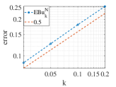
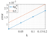
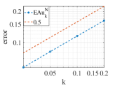
Fig. 1: Time errors of the numerical results at $T=1$ with $h=2^{-7}$.

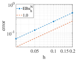
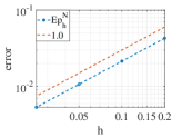
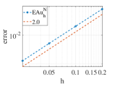
Fig. 2: Spatial errors of the numerical results at $T=1$ with $k=2^{-9}$.

Acknowledgments. The author would like to thank Professor Xiaobing Feng of The University of Tennessee for his many discussions and critical comments as well as valuable suggestions which help to improve the early version of the paper considerably.

References

- [1] A. Bensoussan, Stochastic Navier-Stokes equations, Acta Appl. Math., 38:267–304 (1995).
- [2] A. Bensoussan and R. Temam, Equations stochastiques du type Navier-Stokes, J. Funct. Anal. 13, 195–222 (1973).
- [3] H. Bessaih, Z. Brzeźniak, and A. Millet, Splitting up method for the 2D stochastic Navier-Stokes equations, Stoch. PDE: Anal. Comp., 2:433–470 (2014).
- [4] H. Bessaih and A. Millet, On strong convergence of time numerical schemes for the stochastic 2D Navier-Stokes equations, IMA J. Numer. Anal., 39:2135–2167 (2019).
- [5] D. Breit and A. Dodgson, Convergence rates for the numerical approximation of the 2D stochastic Navier-Stokes equations, Numer. Math., 147:553–578 (2021).
- [6] F. Brezzi and M. Fortin, Mixed and Hybrid Finite Element Methods, Springer, New York, 1991.
- [7] Z. Brzeźniak, E. Carelli, and A. Prohl, Finite element based discretizations of the incompressible Navier-Stokes equations with multiplicative random forcing, IMA J. Numer. Anal., 33:771–824 (2013).
- [8] M. Capiński, A note on uniqueness of stochastic Navier-Stokes equations, Univ. Iagell. Acta Math. 30: 219–228 (1993).
- [9] M. Capiński, N. J. Cutland, Stochastic Navier-Stokes equations, Acta Appl. Math. 25: 59–85 (1991).
- [10] E. Carelli and A. Prohl, Rates of convergence for discretizations of the stochastic incompressible Navier-Stokes equations, SIAM J. Numer. Anal., 50(5):2467–2496 (2012).
- [11] A. Ern and J.-L. Guermond, Theory and Practice of Finite Elements, Springer, 2004.
- [12] P. Dörsek, Semigroup splitting and cubature approximations for the stochastic Navier-Stokes equations, SIAM J. Numer. Anal., 50(2):729–746 (2012).
- [13] R. Falk, A Fortin operator for two-dimensional Taylor-Hood elements, ESAIM: Math. Model. Num. Anal., 42:411–424 (2008).
- [14] X. Feng and H. Qiu, Fully discrete mixed finite element methods for the time-dependent stochastic Stokes equations with multiplicative noise, J. Sci. Comput., 88:1-31 (2021).
- [15] X. Feng, A. Prohl and L. Vo. Optimally convergent mixed finite element methods for the stochastic Stokes equations, IMA J. Numer. Anal., 2021, doi.org/10.1093/imanum/drab006.
- [16] F. Flandoli and D. Gatarek, Martingale and stationary solutions for stochastic Navier-Stokes equations, Probab. Theory Related Fields, 102:367–391 (1995).
- [17] E. Hausenblas and T. Randrianasolo, Time-discretization of stochastic 2D Navier-Stokes equations with a penalty-projection method, Numer. Math., 143:339–378 (2019).
- [18] V. Girault and P.-A. Raviart, Finite Element Methods for Navier-Stokes Equations, Springer, New York, 1986.
- [19] J. A. Langa, J. Real, and J. Simon, Existence and regularity of the pressure for the stochastic Navier-Stokes equations, Appl. Math. Optim., 48:195–210 (2003).
- [20] M. Hairer, J. C. Mattingly, Ergodicity of the 2D Navier-Stokes equations with degenerate stochastic forcing, Ann. Math. 164, 993–1032 (2006).
- [21] S. Kuksin, A. Shirikyan, Mathematics of Two-Dimensional Turbulence, Volume 194 of Cambridge Tracts in Mathematics. Cambridge University Press, Cambridge, 2012.
- [22] G. Da Prato and J. Zabczyk, Stochastic Equations in Infinite Dimensions, Cambridge University Press, Cambridge, UK, 1992.
- [23] R. Temam, Navier-Stokes Equations. Theory and Numerical Analysis, 2nd ed., AMS Chelsea Publishing, Providence, RI, 2001.