Deep Residual Error and Bag-of-Tricks Learning for Gravitational Wave Surrogate Modeling

Abstract

Deep learning methods have been employed in gravitational-wave astronomy to accelerate the construction of surrogate waveforms for the inspiral of spin-aligned black hole binaries, among other applications. We face the challenge of modeling the residual error of an artificial neural network that models the coefficients of the surrogate waveform expansion (especially those of the phase of the waveform) which we demonstrate has sufficient structure to be learnable by a second network. Adding this second network, we were able to reduce the maximum mismatch for waveforms in a validation set by 13.4 times. We also explored several other ideas for improving the accuracy of the surrogate model, such as the exploitation of similarities between waveforms, the augmentation of the training set, the dissection of the input space, using dedicated networks per output coefficient and output augmentation. In several cases, small improvements can be observed, but the most significant improvement still comes from the addition of a second network that models the residual error. Since the residual error for more general surrogate waveform models (when e.g., eccentricity is included) may also have a specific structure, one can expect our method to be applicable to cases where the gain in accuracy could lead to significant gains in computational time.

[inst1]organization=Department of Informatics, Aristotle University of Thessaloniki, city=Thessaloniki, country=Greece [inst2]organization=Department of Physics, Aristotle University of Thessaloniki, city=Thessaloniki, country=Greece

[inst3]organization=GSI Helmholtz Center for Heavy Ion Research, city=64291 Darmstadt, country=Germany

1 Introduction

Observations of GW and the global network of detectors. Since the first detection of gravitational waves (GW) from a system of binary black holes (BBH) in 2015 [1], GW detections have become more and more frequent, approaching gradually the status of routine observations. From that date onwards, GW detections have become more and more frequent, approaching gradually the status of routine observations. The initial observing run (O1) of the two Advanced LIGO [2] laser interferometers based in Hanford and Livingston, resulted in 3 GW events. During the second run (O2) the total number of registered detections increased to 11 (first Gravitational-Wave Transient Catalog, GWTC-1, [3]), with the Advanced Virgo detector [4] joining in towards the end of that observational period. Virgo’s addition to the twin LIGO detectors was paramount, as it coincided with the first detection of a binary neutron star (BNS) coalescence, GW170817 [5], accompanied with extensive observations in the electromagnetic (EM) spectrum [6, 7]. The first part of the third observing run (O3a) updated the number of events to 50 (GWTC-2, [8]), while the latest catalog (GWTC-3, [9]) contains 90 GW events.

Continued improvements in the detectors’ sensitivity [10] are expected to further increase the number of GW observations. A fourth GW observatory, KAGRA [11, 12], joined the global network of GW detectors at the end of the O3 run. KAGRA will participate in the fourth observing run (O4) which is planned to begin in May 2023, while also improving its sensitivity during O4. Additional observatories are important so that the sky localization of GW sources is more accurate and their properties are determined with higher precision, thus providing crucial information for potential EM follow-up observations of GW events. To that end, the construction and operation of a fifth interferometer, LIGO-India [13] will also significantly improve both the network sensitivity and the sky localization. Furthermore, third generation ground-based detectors such as the Einstein Telescope [14, 15] and Cosmic Explorer [16, 17] are actively being developed and they are anticipated to vastly improve our knowledge of astrophysical processes in the Universe [18, 19, 20].

GW modeling. The breakthroughs in GW astronomy briefly described above, were made possible thanks to collaborative efforts on multiple fronts. The rigorous developments in gravitational waveform modeling of a variety of compact binary coalescences (CBC) was undoubtedly a crucial point. A prerequisite to interpret GW signals and unveil the properties of their source is to solve the two-body problem in General Relativity (GR). To that end, one needs to solve the Einstein equations and this can be done either via analytical methods (truncated at some order in a post-Newtonian (PN) expansion, see e.g. [21]) or via numerical solutions of the full Einstein equations (with some assumptions and up to a specified tolerance). The analytical approach is fast, but it is valid only for large separations of the binary and small (compared to the speed of light) orbital velocities, i.e. it breaks down after the late inspiral phase. The subsequent merger and ringdown phase of the coalescence, i.e. the strong field and relativistic velocities regime, can be captured accurately only with numerical relativity (NR). However, the computational cost of such NR simulations (typically performed on supercomputers) is tremendous, ranging from tens of thousands to millions of corehours [22, 23, 24, 25, 26].

Efforts to combine the two aforementioned approaches in order to produce accurate descriptions of the entire coalescence, including the full inspiral, merger and ringdown, have resulted in different families of waveform models. The main ones are the effective-one-body (EOB) and the phenomenological families. The former has two prominent members, the SEOBNR models [27, 28], and the TEOBResum models [29, 30], while the latter comprises of the IMRPhenom models [31, 32].

The EOB approach [33] generalizes to GR the Newtonian result dictating that the relative motion of a two-body system is equivalent to the motion of a particle of mass $\mu=m_{1}m_{2}/(m_{1}+m_{2})$ (where $m_{1}$ and $m_{2}$ are the masses of the binary components) in the two-body potential $V(r)$ . In the EOB context, the PN inspiral information is resummed and calibrated to NR data and the merger-ringdown part is obtained from a fit to NR data. The two EOB subfamilies, SEOBNR and TEOBResum , differ mainly regarding the choices in the resummation process and in the amount of PN and NR information employed.

In the phenomenological approach, the binary coalescence is typically split into 3 regions, where piecewise closed form expressions are used to represent the waveforms. Breaking up the total frequency region into: (i) a low frequency inspiral regime, where the waveform can be described by adding additional terms to a PN expansion, (ii) a high frequency regime, where the waveform is dominated by a quasi-normal ringdown that can be described by perturbation theory and (iii) an intermediate regime, which captures the complex physics of the merger and demands insights from NR, facilitates the finding of appropriate analytical functions. These expressions are fitted to NR waveform data for a set of constructed hybrid waveforms that in essence “glue” together EOB waveforms describing the inspiral and NR waveforms describing the last orbits, merger and ringdown of the binary.

The latest implementations of the EOB and phenomenological families of models include effects from the spin-induced precession of the binary orbit and contributions from both the dominant and subdominant multipole moments of the emitted gravitational radiation. The current state-of-the-art models are SEOBNRv5PHM [28] for the SEOBNR family, IMRPhenomXPHM [32] and IMRPhenomTPHM [34] for the IMRPhenom family and TEOBResumS-GIOTTO [30] for the TEOBResum family. Furthermore, tidal effects can be incorporated [35, 36, 37] in the SEOBNR [38] and IMRPhenom [39] models as appropriate, while in the TEOBResum family tidal and spin effects are merged together into a single EOB framework and therefore no extension is needed as in the other two families.

Progress towards the above cutting-edge waveform models has followed a course of stepping stones along which extra features (i.e. inclusion of spins, higher modes, precession) and different optimization and acceleration techniques were implemented gradually. Early efforts in the EOB front (e.g. [40, 41] resulted in the first versions of the SEOBNR models which evolved from describing non-spinning binaries to spinning, precessing systems. [42, 43, 44, 45]. Improved EOB waveform models soon followed [46, 47, 48, 49, 50] leading up to the 5th and most sophisticated implementation of SEOBNR models [28, 51, 52, 53]. Similarly, groundwork for the IMRPhenom family of waveform models [54, 55] developed to include higher modes [56, 57, 58, 59]. Further improvements in accuracy [60, 61, 62, 63] led to the latest generation of IMRPhenom models [32, 64] becoming a standard tool in GW parameter estimation. The TEOBResum family of models followed a similar course of incremental development [65, 66, 67, 68, 69]. In addition, the expansion of the above waveform family trees from quasi circular to eccentric binaries is diligently pursued [70, 71, 72, 73, 74].

On one hand, the inclusion of extra physical characteristics as outlined above, allows for more realistic and complex waveforms, which is a prerequisite to perform highly accurate parameter estimation of GW sources. Such state-of-the-art models have played a significant role in the analysis of GW from: (i) asymmetric mass binaries [75, 76, 77], (ii) systems whose binary components include one or two neutron stars [78, 79], (iii) GW190521 [80] the most massive BBH merger detected to date [81, 82] and (iv) independent re-analysis of the public LIGO-Virgo-KAGRA (LVK) data, e.g. [83].

On the other hand, the increased complexity decreases the waveforms’ computational efficiency (e.g. compared to the simpler PN approximants). This effect is more pronounced for EOB waveforms, as phenomenological waveforms are faster by construction. The computational cost of EOB models is burdened by the need to tackle the orbital dynamics through solving a complex system of ordinary differential equations. A solution to this problem has been supplied by surrogate modeling [88, 89]. By fitting interpolated decomposed waveform data pieces over the binary parameter space, surrogate models can significantly accelerate either NR (e.g. [90, 91, 92, 93, 94, 95]) or EOB waveforms (e.g. [88, 96, 97, 98, 99]), while maintaining high accuracy within their parameter space of validity.

Motivation and Contribution. In this study, we focus on the SEOBNRv4 model, which has a 3-dimensional parameter space $\boldsymbol{\lambda}$; the mass ratio $q$ between the two BHs and their spins $\chi_{1}$ and $\chi_{2}$, assuming that they are aligned with the orbital angular momentum. Surrogate models have been shown to be fast and reliable approximations of waveforms such as SEOBNRv4, within a specified tolerance error. A surrogate model for this family of waveforms is presented in [100].

As discussed in [100] there are challenges in modeling GW signals and there is a need to reduce computational costs to increase the efficiency of analyzing GW events. While there have been significant advancements in GW signal modeling, incorporating more complex features increases computational costs, limiting their use. To overcome this challenge, custom-made optimizations have been developed [84], but they require expert knowledge and may not provide general optimizations. Alternatively, data-driven methods such as surrogate modeling can be employed, which provide accurate approximations of computationally expensive waveform models [88, 101]. Several machine learning techniques are available for interpolating or fitting the projection coefficients of a reduced basis representation of time-domain waveforms, and the most appropriate method depends on the required accuracy and dimensionality. For low-dimensional parameter spaces, interpolation is a viable option. However, as dimensionality increases, interpolation becomes challenging due to the substantial number of data points usually required. ANNs are proposed to estimate these coefficients since this approach allows for efficient execution on either a CPU or GPU.

In reproducing the results of [100], we noticed that the residual errors after training the neural networks had structure with respect to the input parameters and hypothesized that a second neural network could learn to model these errors. Our contribution can be summarized as follows:

• We design and train a neural network to model the residual errors of the surrogate model network.

• Drawing inspiration from the physical aspect of the task at hand, we introduce various tricks to reduce the learning errors.

• We make use of the residual errors of the training of the ANN model and achieve a maximum mismatch between SEOBNRv4 waveforms and waveforms generated by our surrogate model that is more than one order of magnitude smaller compared to the baseline method.

To the best of our knowledge, this is the first work to model the residual errors of a neural network based gravitational wave surrogate model. The code for this work is available at https://github.com/sfragkoul/residual-gw-surrogate-modelling.

The rest of this paper is arranged as follows: in Section 2 related works are detailed and compared to this work, and in Section 3 surrogate modeling is briefly overviewed, the ground truth used during our experiments is described and the baseline network is presented. In Section 4 we discuss the improvements noticed by adding a supplementary residual error learning network, i.e. a network predicting the errors of the training network. In Section 5 we summarize different approaches investigated to manipulate the input and output space of the networks, aiming to obtain a better mismatch. Section 6 the presentation of how the variants of the ANN surrogate model, as described in the previous sections, perform takes place, and in Section 7 we summarize our findings. Finally, in the Appendix we show additional results for the distribution of the mismatch values for different values of the greedy tolerance.

2 Related Work

Interest in harnessing machine learning techniques for the analysis of GW data has been on the rise lately (see [102] for a review). For example, the interpolation (i.e. the third step described above) can be very costly at high dimensions, in which case probabilistic methods could be employed, see e.g. [103]. In [104] the complex waveforms are separated into the real and imaginary segments and two separate surrogate models are constructed, with artificial neural networks (ANNs) implemented within a 4-dimensional input space to fit the coefficients from the reduced basis, omitting the final step of the empirical interpolation.

In [105], various interpolation methods were investigated, concluding that machine-learning based methods may perform better as the complexity of the surrogate modeling problem increases. In another important development, using genetic programming and symbolic regression techniques, surrogate models based on numerical simulations (i.e. essentially in an ab-initio approach) were used to obtain closed-form expressions for the GW emission of BBH collision, modeling the entire coalescence at once, i.e. without the need to distinguish between the different regimes of inspiral, merger and ringdown [106].

In [100] a time-domain surrogate model of the spin-aligned BBH waveform model SEOBNRv4 [46] was built by utilizing ANNs instead of interpolating during the last step, and also by dividing the problem to the signal parts of the phase and amplitude, which resulted in the creation of two corresponding surrogate models. Furthermore, another recent application of Deep Learning (DL) was implemented [101], where ANNs were used (specifically autoencoders), for the examination of latent structures in the coefficients from the empirical interpolation.

In [107] the authors present the prospect for predicting gravitational waveforms from compact binaries based on automated machine learning (AutoML). The study focuses on the analysis of GW emitted when two spinless black holes collide in an initial quasi-circular orbit. Their findings suggest that AutoML has the potential to serve as a framework for regression in the field of surrogates for gravitational waveforms. Specifically, this research is conducted in the context of surrogates derived from NR simulations using the reduced basis and the empirical interpolation. Their results indicate that AutoML is capable of generating surrogates that closely resemble the actual NR simulations. In [108], the use of ANNs for surrogate modeling is investigated and it is shown that they can be used to build computationally efficient and accurate models for multipolar waveform models of precessing BBHs. The method is applied on the SEOBNRv4PHM waveform model and the generated surrogate model is faster than the original model by 2 orders of magnitude on a CPU. With batched operations and the acceleration of a GPU, this speedup is further increased.

The main advantage of using an ANN-surrogate model in our study is its ability to capture complex nonlinear relationships between the input parameters and the output waveform signals, which can be challenging to model using traditional analytic methods. This approach has been shown to be effective in previous studies for predicting gravitational waveforms [100], and we evaluated the performance of our proposed ANN-surrogate model against a baseline model, which was also based on an ANN architecture. We chose this approach for comparison as it allowed us to assess the effectiveness of our proposed method in improving the accuracy of the predictions relative to a baseline.

Unlike the aforementioned works [100, 101], though, in this study we take into account modeling errors generated by the DL models by learning the residual errors. Furthermore, we draw inspiration from the physical aspect of the task at hand as well as the learning objective, and introduce various tricks to reduce the learning errors. Notably, we make use of the residual errors of the training of the ANN model in order to achieve significantly better results.

3 Background

In the following subsections we provide the theoretical background of surrogate modeling for gravitational waves. Furthermore, we discuss the specifics of constructing an effective surrogate model for the SEOBNRv4 waveform family, following the steps described in [100].

3.1 Construction of a surrogate model

We use the notation $h(t;\boldsymbol{\lambda})=h_{+}(t;\boldsymbol{\lambda})-ih_{\times}(t;\boldsymbol{\lambda})$ to denote a complex gravitational wave strain, where $h_{+}$ and $h_{\times}$ are the two independent polarizations [109], $t$ denotes time and the elements of $\boldsymbol{\lambda}$ are the intrinsic parameters. In general, for inspiraling black holes in general relativity on non-eccentric orbits, these parameters are 7-dimensional, consisting of the mass ratio and two spins with arbitrary orientation. Under restrictions, these parameters can be simplified to only include the mass ratio and two spins aligned with the orbital plane. We study this case, based on the SEOBNRv4 model specifically [46].

Surrogate modeling aims to approximate the given signals using a reduced model, denoted as $h_{s}(t;\boldsymbol{\lambda})$, such that the approximation given by the surrogate model, $h_{s}(t;\boldsymbol{\lambda})$ accurately reconstructs the actual waveform $h(t;\boldsymbol{\lambda})$ within a preset threshold of error. When considering only the dominant, quadrupole ($l=m=2$) mode [109], the target becomes $h_{s}(t;\boldsymbol{\lambda})\approx h_{2,2}(t;\boldsymbol{\lambda})$ where $l,m$ are the spherical harmonics. In surrogate modeling, the first step is to prepare a large training set of waveforms, as previously mentioned. Implementing the SEOBNRv4 model [46], whose input space is three-dimensional, each waveform is parameterized by the mass ratio $q\equiv{m_{1}}/{m_{2}}\geq 1$ and the dimensionless spins $\chi_{1},\chi_{2}$ of the two black holes. Thus, a training set of $N$ waveforms $\{h_{i}(t;\boldsymbol{\lambda}_{i})\}_{i=1}^{N}$ is created, where ${\boldsymbol{\lambda}}_{i}=(q,\chi_{1},\chi_{2})_{i}$. The mass ratio is limited to a predetermined interval, e.g. as $1\leq q\leq 8$, inside which the surrogate model is accurate by design. For the two spins, their values can be in the range $-0.99\leq\chi_{1,2}\leq 0.99$.

A reduced basis is built from the training set, using either a greedy algorithm [88] or algebraic approaches, like Singular Value Decomposition (SVD) [91]. The greedy algorithm is an iterative process, which chooses $n<N$ waveforms (and, by extension, their corresponding ${\{\boldsymbol{\lambda}}_{j}\}_{j=1}^{n}$ values, the greedy points), which, after orthonormalization, constitute the reduced basis $\{e_{j}\}_{j=1}^{n}$. Each $\boldsymbol{\lambda}_{i}$ waveform in the training set is then represented as a linear combination

$$h(t;\boldsymbol{\lambda}_{i})\approx\sum_{j=1}^{n}c_{j}(\boldsymbol{\lambda}_{i})e_{j}(t),$$ (1)

within a preset error tolerance, where $\{c_{j}(\boldsymbol{\lambda}_{i})\}_{j=1}^{n}=\left\langle h(t;\boldsymbol{\lambda}_{i}),e_{j}(t)\right\rangle$ are the orthogonal projection coefficients. To ensure that our coefficients remain smooth with respect to the parameters, we adopted measures to mitigate the impact of noisy data. Specifically, we employed a higher sampling rate and a larger number of training samples, which enabled us to obtain a smooth and dense input parameter space. Furthermore, our data are generated by highly-accurate semi-analytic waveform models, so they do not suffer from experimental data noise – any numerical data noise is orders of magnitude smaller than the mismatch we are aiming for. Our approach is in line with the recommendations put forth by [88].

Next, a new EIM basis $B_{k}(t)$ is obtained, such that a waveform $h(t;\boldsymbol{\lambda}_{j})$ (where $\boldsymbol{\lambda}_{j}$ is one of the greedy points of the ROM basis) can be represented as the linear combination

$$h\left(t;\boldsymbol{\lambda}_{j}\right)=\sum_{k=1}^{n}\alpha_{k}(\boldsymbol{\lambda}_{j})B_{k}(t),$$ (2)

where the coefficients $\alpha_{k}(\boldsymbol{\lambda}_{j})$ coincide with the waveform at particular times, $\{T_{k}\}_{k=1}^{n}$, the empirical time nodes, i.e. $\alpha_{k}(\boldsymbol{\lambda}_{j})=h\left(T_{k};\boldsymbol{\lambda}_{j}\right)$.

For any other waveform $h\left(t;\boldsymbol{\lambda}_{i}\right)$ in the training set, the coefficients of the EIM representation are simply $\alpha_{k}(\boldsymbol{\lambda}_{i})=h\left(T_{k};\boldsymbol{\lambda}_{i}\right)$. Since this does not involve the basis $B_{k}(t)$, the coefficients are computed much faster (as known values of the waveform at particular times) than the projection coefficients in the ROM basis (which require the projection of the whole waveform).

A surrogate model is finally produced, by interpolating over the coefficient matrix $\alpha_{k}(\boldsymbol{\lambda}_{i})$ of the training set to find the coefficients $\hat{\alpha}_{k}(\boldsymbol{\lambda})$ for an arbitrary $\boldsymbol{\lambda}$, such that

$$h\left(t;\boldsymbol{\lambda}\right)\approx\sum_{k=1}^{m}\hat{\alpha}_{k}(\boldsymbol{\lambda})B_{k}(t).$$ (3)

Depending on the dimensionality of $\boldsymbol{\lambda}$, multi-dimensional interpolation is required, the computational cost of which increases dramatically with increasing number of parameters. This particular part of the process can be accelerated using neural networks, as shown in [100].

In practice, we used a similar setup as in [100], as our baseline model. Instead of working with the strain amplitudes $h_{+}$ and $h_{\times}$, we use the amplitude $A$ and phase $\phi$ of the complex waveform, defined through

$$h_{+}\left(t;\boldsymbol{\lambda}\right)-h_{\times}\left(t;\boldsymbol{\lambda}\right)=A\left(t;\boldsymbol{\lambda}\right)e^{-i\phi\left(t;\boldsymbol{\lambda}\right)},$$ (4)

as this results in a more compact EIM basis. The training set comprised $N=2\times 10^{5}$ waveforms, randomly sampled in the $1\leq q\leq 8,-0.99\leq\chi_{1,2}\leq 0.99$ parameter space. The waveforms in the training set were accurately aligned in amplitude and initial phase, the phase was unwrapped and the time series was truncated to correspond to a common starting time of $-20000M$, where we chose a total mass of $M=60M_{\odot}$. This ensured that all waveforms started with a minimum frequency no larger than 15 Hz. We kept $100M$ of post-peak ringdown data. The ROM and EIM bases were constructed using RomPy [88, 112].

A validation set of $3\times 10^{4}$ SEOBNRv4 waveforms (not included in the training set) was used to evaluate the accuracy of the reconstructed waveforms.

3.2 Measuring the reconstruction error

For two waveforms with parameters $\boldsymbol{\lambda}_{1}$ and $\boldsymbol{\lambda}_{2}$, one defines the inner product [113]

$$\langle h(\cdot;\boldsymbol{\lambda}_{1}),h(\cdot;\boldsymbol{\lambda}_{2})\rangle=4\Re\int_{f_{min}}^{f_{max}}\frac{\tilde{h}(f;\boldsymbol{\lambda}_{1})\tilde{h}^{*}(f;\boldsymbol{\lambda}_{2})}{S_{n}(f)}df,$$ (5)

where $\tilde{h}(f;\boldsymbol{\lambda})$ is the Fourier transform of $h(t;\boldsymbol{\lambda})$, $S_{n}(f)$ denotes the noise power spectral density (PSD) of the GW detector and the star notation denotes the complex conjugate. The inner product can be used to normalise the Fourier transform of a waveform as

$$\hat{h}(f;\boldsymbol{\lambda})=\frac{{\tilde{h}}(f;\boldsymbol{\lambda})}{\langle h(\cdot;\boldsymbol{\lambda}),h(\cdot;\boldsymbol{\lambda})\rangle},$$ (6)

Then, the overlap between two waveforms is defined as the inner product between normalised waveforms $\hat{h}(\cdot;\boldsymbol{\lambda}_{1})$, $\hat{h}(\cdot;\boldsymbol{\lambda}_{2})$, maximised over a relative time ($t_{0}$) and phase ($\phi_{0}$) shift between the two waveforms:

$${\cal O}(\hat{h}(\cdot;\boldsymbol{\lambda}_{1}),\hat{h}(\cdot;\boldsymbol{\lambda}_{2}))=\max_{t_{0},\phi_{0}}\langle h(\cdot;\boldsymbol{\lambda}_{1}),h(\cdot;\boldsymbol{\lambda}_{2})\rangle,$$ (7)

and, finally the mismatch is given by

$$\mathcal{M}(\hat{h}(\cdot;\boldsymbol{\lambda}_{1}),\hat{h}(\cdot;\boldsymbol{\lambda}_{2}))=1-{\cal O}(\hat{h}(\cdot;\boldsymbol{\lambda}_{1}),\hat{h}(\cdot;\boldsymbol{\lambda}_{2})).$$ (8)

To measure the performance of the surrogate model, the mismatch between actual waveforms, given by the SEOBNRv4 model, and surrogate predictions is used.

Table 1: Number of coefficients ($n$) of the reduced EIM bases for the amplitude and phase for different values of the greedy tolerance. The last three columns show the mismatch $\mathcal{M}$ (maximum, median and $95^{\rm th}$ percentile values) of the waveforms in the validation set when reconstructed via Eq. (2).

Greedy	$n$	$n$		mismatch $\mathcal{M}$
Tolerance	(amplitude)	(phase)	(max)	(median)	($95^{\rm th}$ percentile)
$10^{-6}$	$8$	$4$	$8.44\times 10^{-3}$	$5.47\times 10^{-4}$	$1.81\times 10^{-3}$
$10^{-8}$	$13$	$4$	$8.44\times 10^{-3}$	$5.45\times 10^{-4}$	$1.80\times 10^{-3}$
$10^{-10}$	$18$	$8$	$4.95\times 10^{-4}$	$1.30\times 10^{-5}$	$8.22\times 10^{-5}$
$10^{-12}$	$41$	$12$	$2.07\times 10^{-6}$	$7.45\times 10^{-8}$	$2.83\times 10^{-7}$
$10^{-14}$	$84$	$32$	$1.34\times 10^{-8}$	$5.64\times 10^{-10}$	$3.95\times 10^{-9}$
$10^{-16}$	$93$	$48$	$6.60\times 10^{-9}$	$4.59\times 10^{-10}$	$3.02\times 10^{-9}$

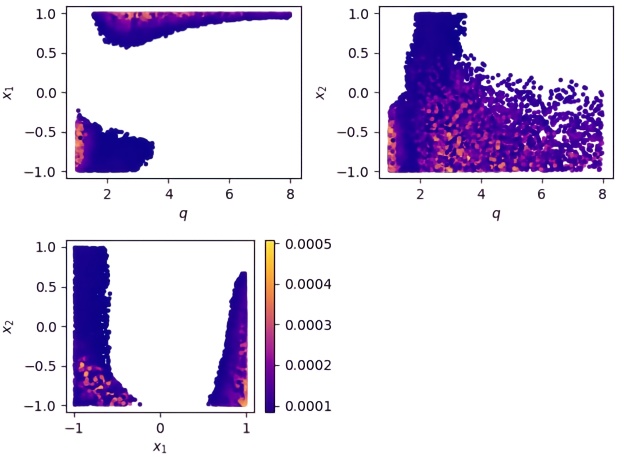
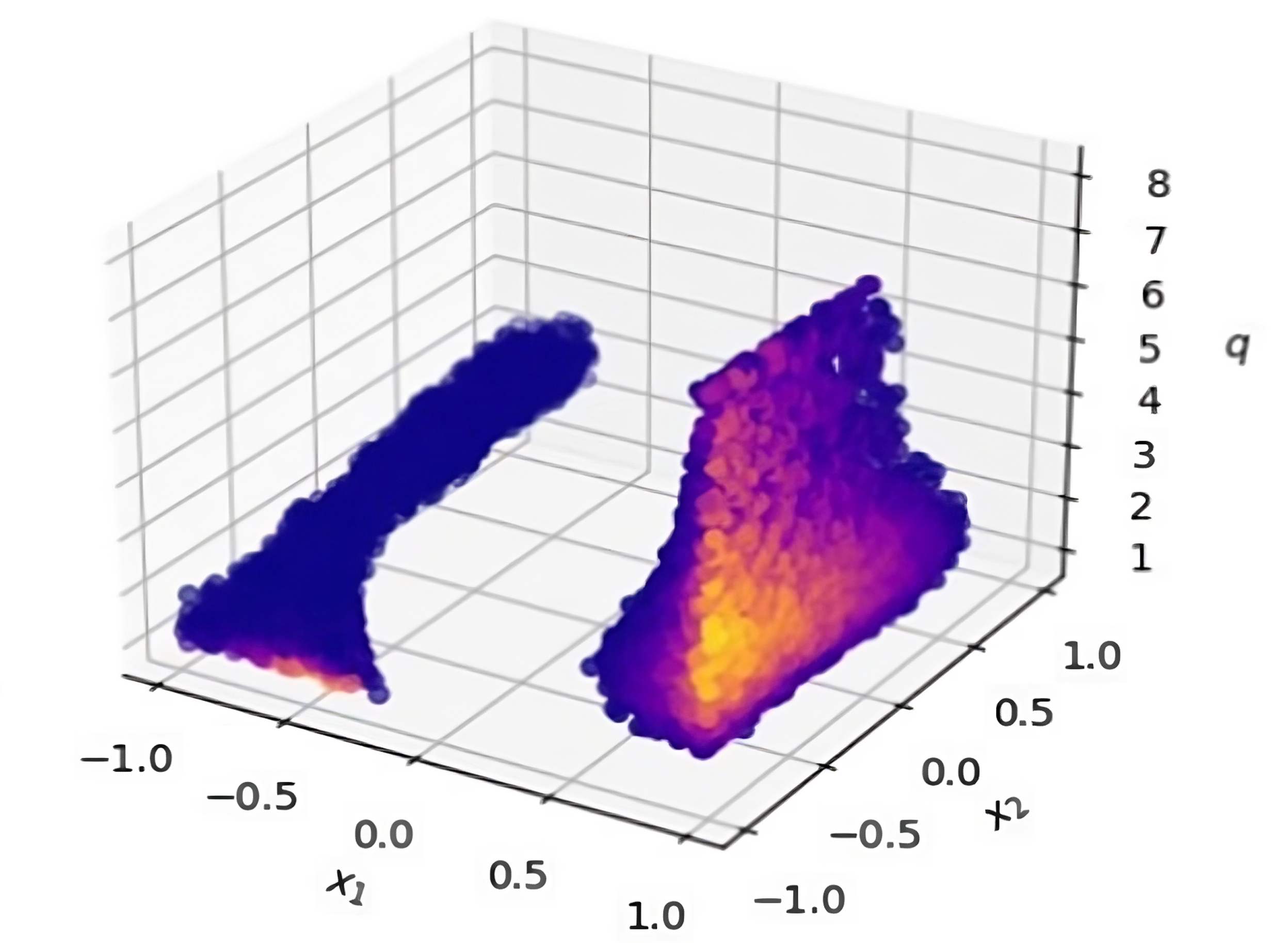
Figure 1: Two-dimensional and three-dimensional distribution of mismatch values larger than $\sim 8\times 10^{-5}$ ($95^{th}$ percentile) for the waveforms in the training set, when reconstructed using the EIM reduced basis via Eq. (2), with a greedy tolerance of $10^{-10}$.

3.3 Performance of the reduced basis reconstruction and ground truth

Table 1 shows the number of coefficients of the reduced EIM basis for the amplitude and for the phase for different values of the greedy tolerance. The last three columns show the maximum, median and $95^{\rm th}$ percentile mismatch of the waveforms in the validation set when reconstructed via Eq. (2). An initial greedy tolerance of $10^{-6}$ results in a basis with just 8 coefficients for the amplitude and 4 coefficients for the phase, with a median mismatch of the ANN surrogate model of $\simeq 5\times 10^{-4}$. Decreasing the greedy tolerance to $10^{-10}$ reduces the median mismatch to $\simeq 10^{-5}$, requiring 18 coefficients for the amplitude and 8 coefficients for the phase. With even lower greedy tolerances, one can reach a median mismatch of only $\simeq 5\times 10^{-10}$ at the expense of a larger number of coefficients. The results in Table 1 are comparable to the corresponding results in Table I of [100].

For the case of a greedy tolerance of $10^{-10}$, the two-dimensional and three-dimensional distributions of mismatch values larger than $\sim 8\times 10^{-5}$ ($95^{th}$ percentile) for the waveforms in the training set, when reconstructed using the EIM reduced basis via Eq. (2), are shown in Fig. 1. The corresponding distributions for the validation set and for various values of the greedy tolerance are shown in the Appendix. The distributions are different at very small values of the greedy tolerance, when compared to the distributions for higher values of the greedy tolerance.

Next, selecting a greedy tolerance of $10^{-10}$, the $k=18$ coefficients $\alpha_{k}(\boldsymbol{\lambda}_{i})=h\left(T_{k};\boldsymbol{\lambda}_{i}\right)$ for the amplitude and corresponding 8 coefficients for the phase (for each of the $N=2\times 10^{5}$ waveforms with parameters $\boldsymbol{\lambda}_{i}$ in the training set) were used as the ground truth for the baseline ANN surrogate model discussed in the next subsection. In the remainder of this paper, we will denote the ground truth EIM coefficients of the $N$ training set waveforms as $\boldsymbol{y}_{i}\equiv\{\alpha_{k}(\boldsymbol{\lambda}_{i})\}_{k=1}^{n}$.

3.4 ANN surrogate model: the baseline network

To complete the surrogate model, an ANN was trained to interpolate the coefficients $\alpha_{k}({\boldsymbol{\lambda}_{i}})$ of the training set to find the coefficients $\hat{\alpha}_{k}(\boldsymbol{\lambda})$ for an arbitrary $\boldsymbol{\lambda}$. We implemented the idea and baseline ANN model which followed the architecture from [100] and compared our proposed model with this baseline. There were 4 hidden layers with 320 neurons in each. The batch size was $10^{3}$ and the training lasted for $10^{3}$ epochs. For the amplitude network we used the Adam optimizer [115] with a learning rate of $10^{-3}$ and the activation function was ReLU [116]. For the phase network, we used the Adamax [115] optimizer with a learning rate of $10^{-2}$ and the activation function was softplus [117]. It is worth mentioning that in preliminary experiments various hyperparameters which affect the training process, including learning rate, optimizer type, batch size and learning rate schedule were tested. The best performing set of hyperparameters in terms of MSE on our validation set were finally chosen for the baseline model. As far as preprocessing is concerned, in both cases $\log(q)$ was used as an input instead of $q$, which was then scaled using the StandardScaler from Scikit-Learn [118]. At the output, the coefficients were used raw for the amplitude network and were scaled using Scikit-Learn’s MinMaxScaler for the phase network. All experiments were conducted on an NVIDIA RTX 2080 Ti GPU.

Table 2: Mean square error (MSE) of the predictions of the ANN surrogate model for the training set and for the validation set, for the baseline network.

	MSE for training set	MSE for validation set
	(average of 5 runs)	(average of 5 runs)
Amplitude	$1.79\times 10^{-7}\pm 3.52\times 10^{-10}$	$1.84\times 10^{-7}\pm 3.29\times 10^{-10}$
Phase	$1.05\times 10^{-8}\pm 2.18\times 10^{-10}$	$1.06\times 10^{-8}\pm 2.11\times 10^{-10}$

The ANN prediction of the EIM coefficients of the training set waveforms will be denoted as $\hat{\boldsymbol{y}}_{i}\equiv\{\hat{\alpha}_{k}(\boldsymbol{\lambda}_{i})\}_{k=1}^{n}$. During training, the standard mean square error

$$MSE=\frac{1}{N}\sum_{i=1}^{N}\|\hat{\boldsymbol{y}}_{i}-\boldsymbol{y}_{i}\|_{2}^{2}$$ (9)

was measured and minimized, where the $\|\cdot\|_{2}$ notation represents the Euclidean norm of a vector. Table 2 displays the MSE (average of 5 runs) of the predictions of the ANN surrogate model for the training set and the corresponding predictions for the validation set, for the baseline network. The MSEs are in the range $\sim 10^{-8}-10^{-7}.$ During our experiments it was observed that the amplitude required less epochs to converge (about 400) whereas the phase network always took more (about 800). Throughout our ablation study, we closely monitored the behavior of both the MSE and the mean absolute error (MAE). After careful consideration, we determined that these metrics exhibit similar trends. As a result, we chose to report the MSE in our experiments, as it is the objective function that we utilized to train our ANNs.

In Table 3 we display the calculated mismatch $\mathcal{M}$ of the predictions of the baseline network for the validation set (average of 5 runs) in order to outline how we evaluated the performance of our ANN surrogate model by comparing the mismatch of the generated waveforms with the original waveforms from the SEOBNRv4 model, which served as our benchmark for accuracy assessment. The maximum mismatch is $7.73\times 10^{-3}$, the $95^{\text{th}}$ percentile is $2.95\times 10^{-4}$ and the median mismatch is $8.39\times 10^{-5}$. These values are only several times (less than an order of magnitude) larger than the corresponding mismatch values for the ground truth in Table 1, demonstrating that the ANN surrogate model can predict waveforms for arbitrary $\boldsymbol{\lambda}$ (within the training ranges) with good accuracy.

The two-dimensional and three-dimensional distributions of mismatch values larger than $\sim 3\times 10^{-4}$ ($95^{th}$ percentile) are shown in Fig. 2. Similarly to the ground-truth distributions of Fig. 1, large mismatches are seen primarily for high spin values and at the corners and edges of the two-dimensional distributions.

Table 3: Mismatch $\mathcal{M}$ of the predictions of the baseline network for the validation set (average of 5 runs). The minimum, maximum, $95^{\text{th }}$ percentile and median mismatch are shown.

	Mismatch $\mathcal{M}$
	(average of 5 runs)
Min	$2.70\times 10^{-6}\pm 3.43\times 10^{-7}$
Max	$7.73\times 10^{-3}\pm 5.38\times 10^{-4}$
$95^{\text{th }}$	$2.95\times 10^{-4}\pm 6.61\times 10^{-6}$
Median	$8.39\times 10^{-5}\pm 1.91\times 10^{-6}$

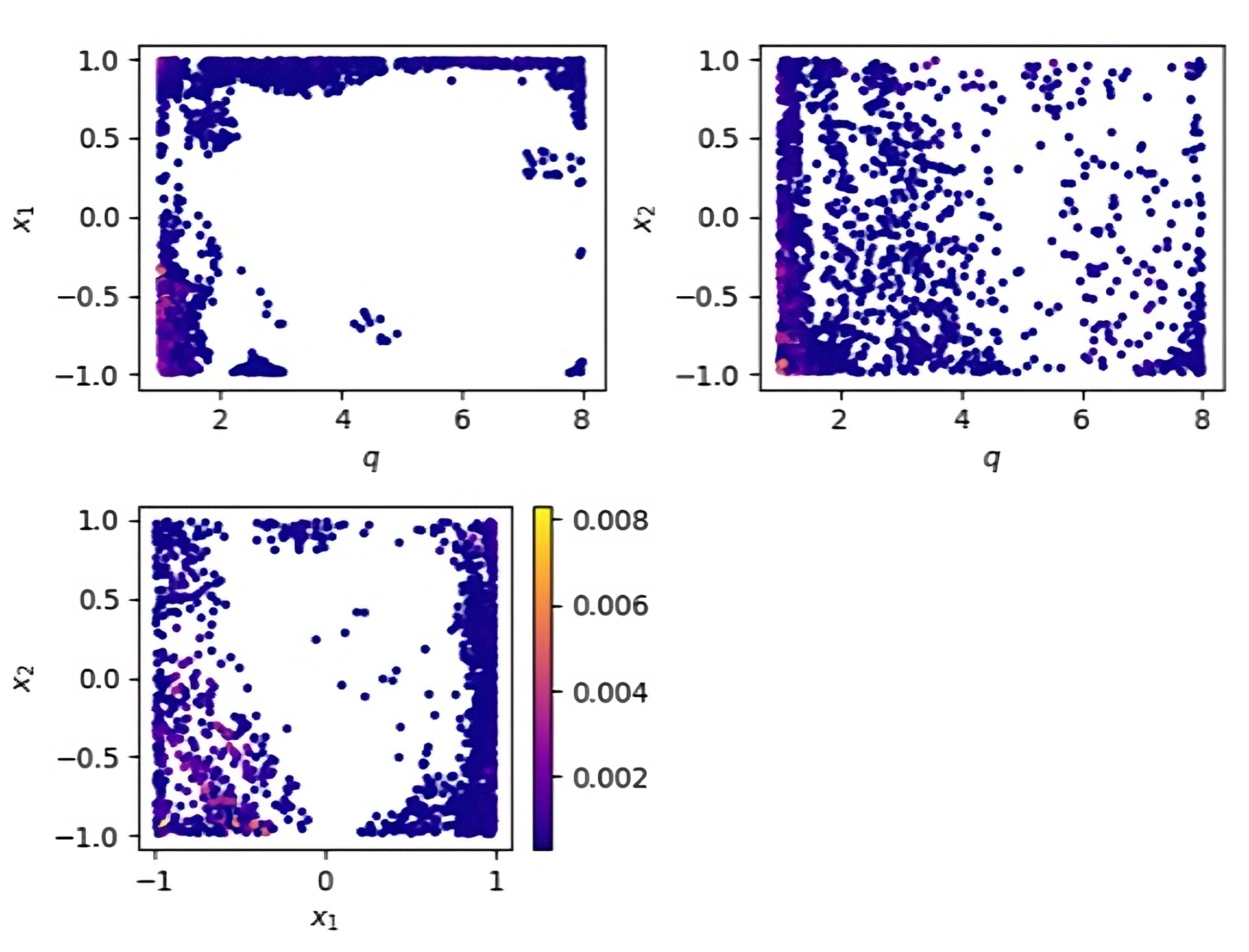
Figure 2: Two-dimensional and three-dimensional distribution of mismatch values larger than $\sim 3\times 10^{-4}$ ($95^{th}$ percentile) of the predictions of the baseline network for the waveforms in the validation set.

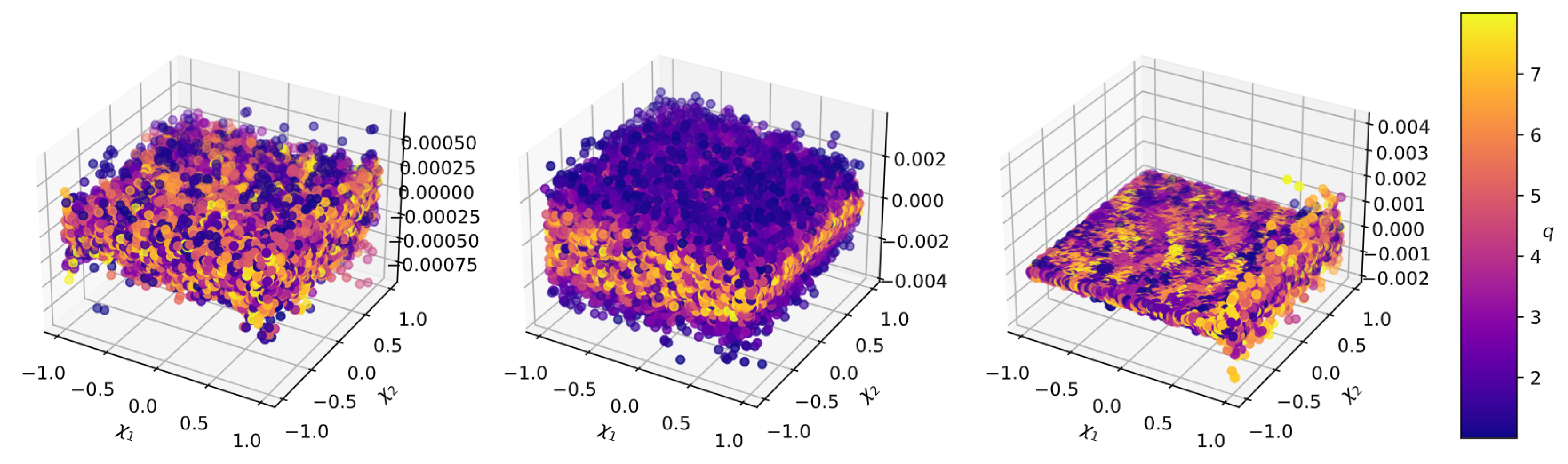
Figure 3: Dependence of the residual error for three selected EIM coefficients for the amplitude on the input parameters $\boldsymbol{\lambda}=\{\chi_{1},\chi_{2},q\}$ (the dependence on $q$ is shown using a colormap). The example in the middle panel shows a strong dependence on the mass ratio $q$, whereas the example on the right shows a large residual error at the largest value of $\chi_{1}$.

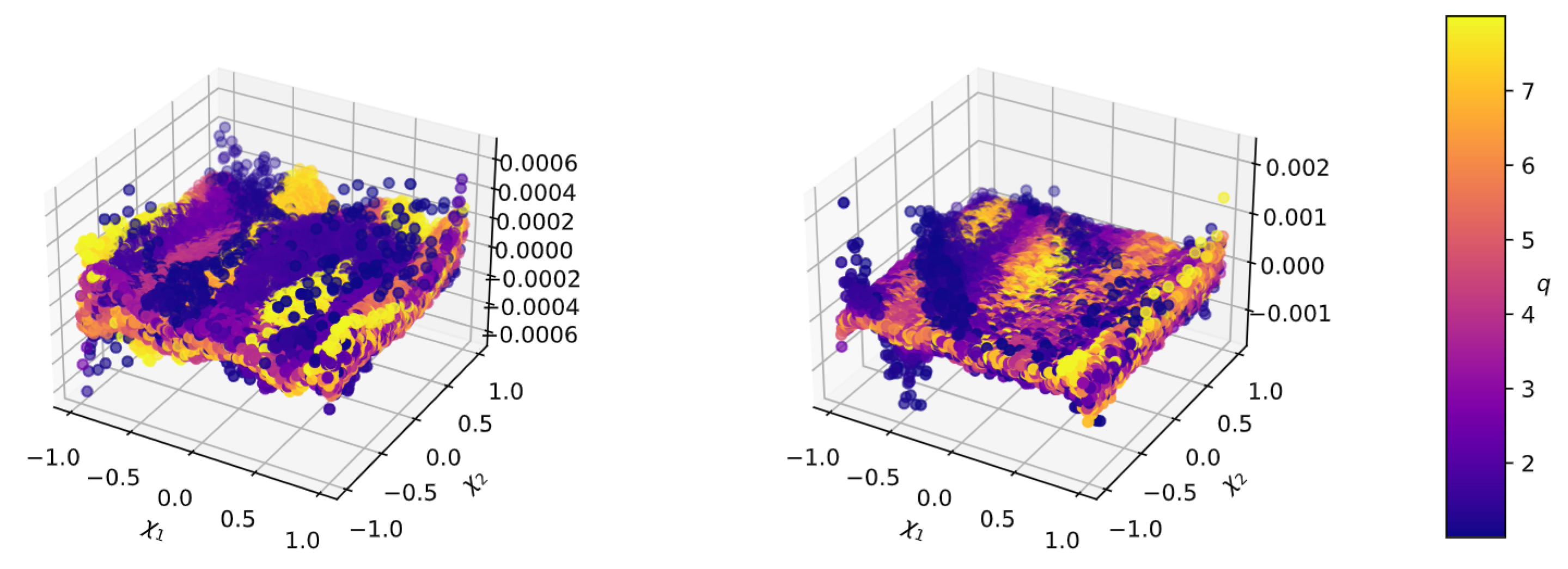
Figure 4: Dependence of the residual error for two selected EIM coefficients for the phase on the input parameters $\boldsymbol{\lambda}=\{\chi_{1},\chi_{2},q\}$ (the dependence on $q$ is shown using a colormap). Some clustering of the errors as a function of the mass ratio can be seen.

3.4.1 Baseline model architecture exploration

Another direction that was explored was that of the architecture of the baseline model. Two types of experiments were tried out, one of shallower models and one of deeper. Both the number of hidden layers and nodes per hidden layer were part of this experimentation. Specifically, for the shallow networks three scenarios were put to test, the input and output layers were kept the same but the hidden layers were altered to a) a single layer with 160 nodes, b) 2 layers with 320 nodes each, c) 4 layers with 160 nodes and for the deeper architecture version hidden layers were altered to a) 4 layers with 640 nodes and b) 8 layers with 320 nodes each. The final mismatches for these experiments are presented in Table 4 and their corresponding violin plots are shown in Figure 5. We choose violin plots with a logarithmic scale to visually compare the methods, as the errors are very small and cover several orders of magnitude. All of the evaluated architectures achieve more or less the same results, with one exception: the shallow network with one layer of 160 neurons performs significantly worse.

Table 4: Mismatch $\mathcal{M}$ of the predictions of the different architectures of the baseline network for the validation set (average of 5 runs). The maximum, $95^{\text{th }}$ percentile and median mismatch are shown.

	Mismatch $\mathcal{M}$ (average of 5 runs)
	Max	$95^{\rm th}$ percentile	Median
baseline	$7.73\times 10^{-3}\pm 5.38\times 10^{-4}$	$2.95\times 10^{-4}\pm 6.61\times 10^{-6}$	$8.39\times 10^{-5}\pm 1.91\times 10^{-6}$
1x160	$2.00\times 10^{-1}\pm 7.59\times 10^{-3}$	$2.65\times 10^{-2}\pm 9.54\times 10^{-4}$	$4.77\times 10^{-3}\pm 1.68\times 10^{-4}$
2x320	$8.84\times 10^{-3}\pm 1.31\times 10^{-3}$	$3.07\times 10^{-4}\pm 3.85\times 10^{-5}$	$7.43\times 10^{-5}\pm 6.88\times 10^{-6}$
4x160	$4.57\times 10^{-3}\pm 7.11\times 10^{-4}$	$8.51\times 10^{-4}\pm 4.75\times 10^{-4}$	$2.65\times 10^{-4}\pm 1.47\times 10^{-4}$
4x640	$8.44\times 10^{-3}\pm 2.94\times 10^{-3}$	$3.07\times 10^{-4}\pm 2.07\times 10^{-5}$	$8.67\times 10^{-5}\pm 2.39\times 10^{-6}$
8x320	$8.39\times 10^{-3}\pm 1.59\times 10^{-3}$	$2.89\times 10^{-4}\pm 1.71\times 10^{-5}$	$7.69\times 10^{-5}\pm 2.64\times 10^{-6}$

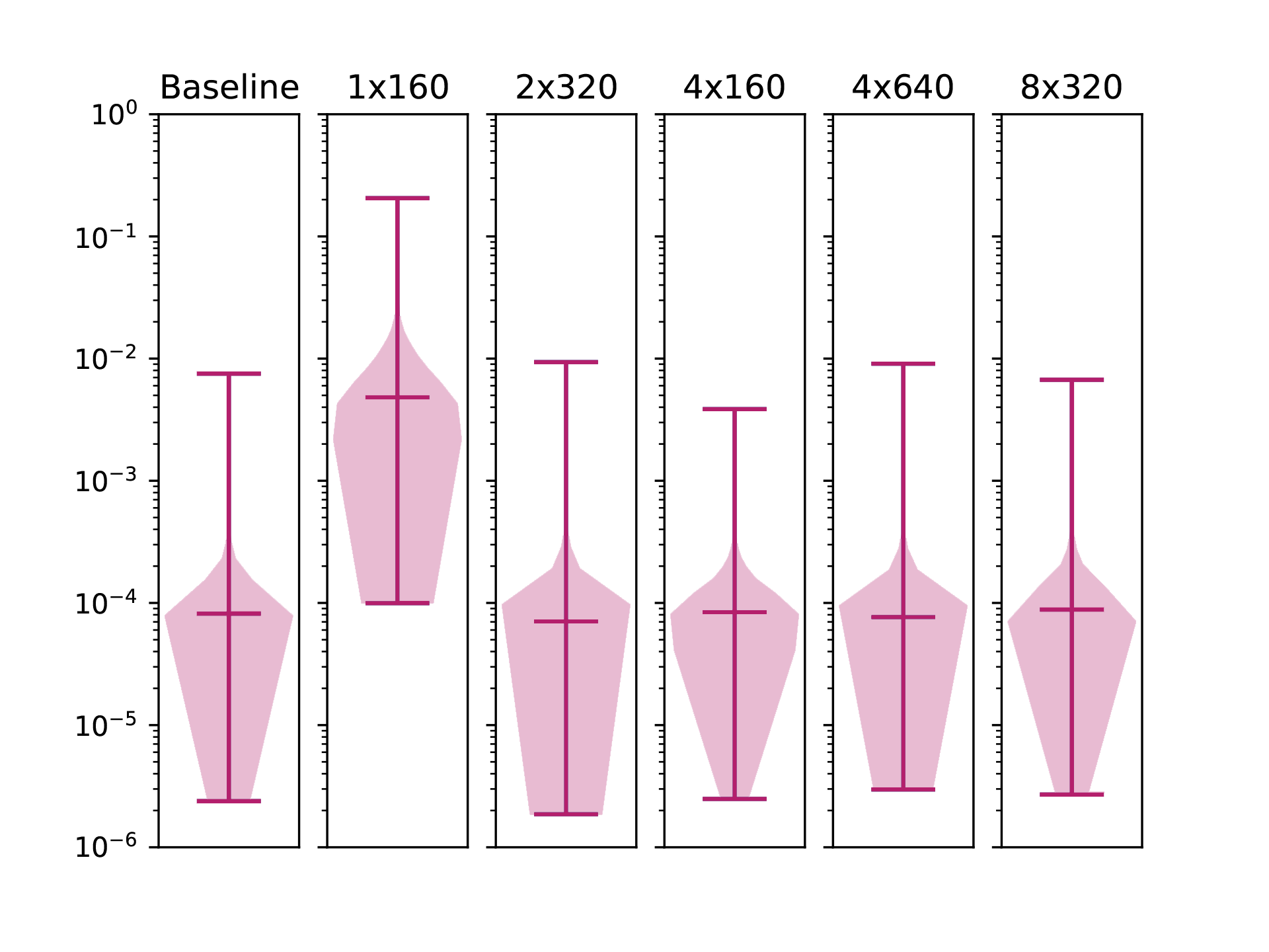
Figure 5: Violin plots comparing the mismatches (for the validation set) between the various baseline network architectures. The middle horizontal line marks the median and the extent of the lines show the minimum and maximum values. In each panel, the envelope is proportional to the density of points. Above the plots the first number corresponds to the number of hidden layers while the second is the number of nodes in each hidden layer.

4 Improvement through Residual Errors Network

Having established the baseline ANN surrogate model in Sec. 3.4, we proceeded in implementing and evaluating three different pathways for improving the mismatch. First, by using a residual error modeling approach, second, using auxiliary tasks to avoid overfitting, and finally by constructing a feature space that can be better exploited by DL models. The implemented pipeline is outlined in Figure 6. Both models take as input the parameters $\boldsymbol{\lambda}$. The baseline models are trained first, to predict amplitude and phase coefficients. Then, the residual errors are computed as shown in Eq. (10) and the residual model is trained to predict these. The final predictions are the sum of the outputs of the two models.

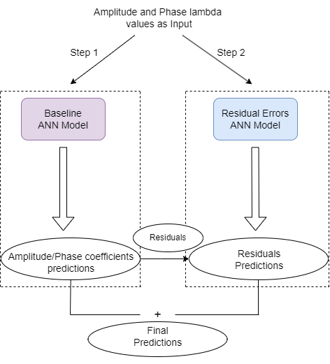
Figure 6: A block diagram of the implemented models.

The first improvement (which also turned out to be the most significant) was obtained by adding a second network (after the training) which can make predictions for the errors of the first network. We remind that for the baseline model, the first network had three-dimensional input $\{\boldsymbol{\lambda_{i}}\}_{i=1}^{N}$ and produced predictions $\hat{\boldsymbol{y}}(\boldsymbol{\lambda})$ (for an arbitrary $\boldsymbol{\lambda}$) with 18 dimensions for the amplitude and 8 for the phase network. For all $\{\boldsymbol{\lambda}_{i}\}_{i=1}^{N}$ in the training set, one can obtain the corresponding predictions {$\hat{\boldsymbol{y}}(\boldsymbol{\lambda}_{i})\}_{i=1}^{N}$ and calculate the residual

$$\boldsymbol{e}_{i}\equiv\boldsymbol{y}(\boldsymbol{\lambda}_{i})-\hat{\boldsymbol{y}}(\boldsymbol{\lambda}_{i}),$$ (10)

where, as already defined, $\boldsymbol{y}$ is the ground truth. Note that the input $\boldsymbol{\lambda}$ undergoes various transformations before being fed to the network, including logarithmic transform of q, and min-max normalization. The second network was designed to have the same input and architecture as the first network, but this time it was trained on the residuals $\boldsymbol{e}_{i}$ (which were first scaled using “MinMaxScaler” from scikit-learn [118]) to make predictions for the residual $\hat{\boldsymbol{e}}(\boldsymbol{\lambda})$ at an arbitrary $\boldsymbol{\lambda}$. For this second network the MSE was defined as

$$MSE=\frac{1}{N}\sum_{i=1}^{N}\|\hat{\boldsymbol{e}}_{i}-\boldsymbol{e}_{i}\|_{2}^{2}.$$ (11)

Adding the prediction $\hat{\boldsymbol{e}}$ for the residual to the prediction $\hat{\boldsymbol{y}}$ of the first network, one obtains an improved prediction

$$\tilde{\boldsymbol{y}}\equiv\hat{\boldsymbol{y}}+\hat{\boldsymbol{e}}.$$ (12)

Table 5: Mean square error (MSE) of the predictions of the ANN surrogate model for the amplitude and phase of the validation set, using the baseline network (middle column) and when a second network that models the residual error is added (right column). In the second case, the MSE of the phase is reduced by a factor of $~{}\sim 5$.

	MSE for baseline network	MSE with residual network
	(average of 5 runs)	(average of 5 runs)
amplitude	$1.84\times 10^{-7}\pm 1.90\times 10^{-10}$	$1.80\times 10^{-7}\pm 2.74\times 10^{-10}$
phase	$1.08\times 10^{-8}\pm 2.11\times 10^{-10}$	$1.93\times 10^{-9}\pm 1.58\times 10^{-12}$

Table 6: Mismatch $\mathcal{M}$ of the predictions of the baseline network (middle column) and when a second network that models the residual error is added (right column), for the validation set (average of 5 runs). The minimum, maximum, $95^{\text{th }}$ percentile and median mismatches are shown.

	Mismatch $\mathcal{M}$	Mismatch $\mathcal{M}$
	(average of 5 runs)	(average of 5 runs)
	baseline network	with residual network
Min	$2.70\times 10^{-6}\pm 3.43\times 10^{-7}$	$1.78\times 10^{-7}\pm 2.34\times 10^{-8}$
Max	$7.73\times 10^{-3}\pm 5.38\times 10^{-4}$	$5.75\times 10^{-4}\pm 1.14\times 10^{-5}$
$95^{\text{th }}$	$2.95\times 10^{-4}\pm 6.61\times 10^{-6}$	$1.33\times 10^{-4}\pm 1.01\times 10^{-7}$
Median	$8.39\times 10^{-5}\pm 1.91\times 10^{-6}$	$4.33\times 10^{-5}\pm 2.73\times 10^{-8}$

It is worth noting that the residual errors $\boldsymbol{e}_{i}$ for the EIM coefficients of the $N$ waveforms in the training set are not always distributed randomly, but can show a certain structure. Fig. 3 displays the dependence of the residual error for three selected EIM coefficients for the amplitude on the input parameters $\boldsymbol{\lambda}=\{\chi_{1},\chi_{2},q\}$ (the dependence on $q$ is shown using a colormap). The example in the middle panel shows a strong dependence on the mass ratio $q$, whereas the example on the right shows a large residual error at the largest value of $\chi_{1}$. The distribution of the residual errors for other coefficients in the EIM expansion is quite similar to one of these characteristic cases. Fig. 4 shows the corresponding dependence of the residual error for two selected EIM coefficients for the phase. Some clustering of the errors as a function of the mass ratio can be seen, which is a strong indication that a second network can learn the residual error.

Table 5 displays the mean square error (MSE) of the predictions of the ANN surrogate model for the amplitude and phase of the validation set, using the baseline network (middle column) and when a second network that models the residual error is added (right column). For the amplitude there is only minimal improvement, but for the phase, the addition of the second network that models the residual error reduces the MSE of the predictions for the validation set by a considerable factor of $~{}\sim 5$.

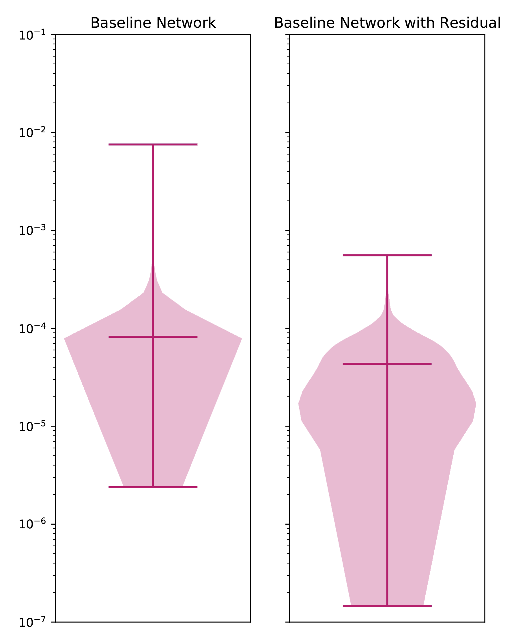
Figure 7: Violin plots comparing the mismatches (for the validation set) between the baseline network and the case when a second network that models the residual error is added. The middle horizontal line marks the median and the extent of the lines show the minimum and maximum values. In each panel, the envelope is proportional to the density of points. A significant reduction of the mismatch is achieved when the network for the residual error is added.

In Table 6, we display the mismatch $\mathcal{M}$ of the predictions of the baseline network (middle column) and when a second network that models the residual error is added (right column), for the validation set (average of 5 runs). In the second case, the minimum error is reduced by a factor of $\sim 15$, the maximum error by a factor of $\sim 13$, and the $95^{\text{th }}$ percentile and median by a factor of $\sim 2$. Fig. 7 compares the mismatches (for the validation set) between the baseline network and the case when a second network that models the residual error is added, as a violin plot. The middle horizontal line marks the median and the extent of the lines show the minimum and maximum values. In each panel, the envelope is proportional to the density of points.

The significant improvements in the mismatch shown in Table 6 and Fig. 7 demonstrate that adding a second network that learns the residual errors is indeed beneficial to the construction of surrogate models for gravitational waves from BBH inspiral. There is good reason to hope that this strategy will also prove to be beneficial for other types of GW template banks, such as binary neutron star inspiral waveforms.

4.1 Effect of residual network on different baseline architecture models

The idea of residual errors network was also tried during the experiments which concerned the architecture of the baseline model. In all cases the architecture of the residual errors network was not altered and kept with 4 hidden layers with 320 nodes in each one of them. The final mismatches for these experiments with the addition of the residual errors network are presented in Table 7 and their corresponding violin plots are shown in Figure 8. As shown the best choice for baseline model is that of 4 hidden layers with 320 nodes in each of them, followed by a residual errors network with the same architecture.

Table 7: Mismatch $\mathcal{M}$ of the predictions of the different architectures of the baseline network for the validation set (average of 5 runs) with the effect of the residual errors network. The maximum, $95^{\text{th }}$ percentile and median mismatch are shown.

	Mismatch $\mathcal{M}$ (average of 5 runs)
	Max	$95^{\rm th}$ percentile	Median
baseline	$5.75\times 10^{-4}\pm 1.14\times 10^{-5}$	$1.33\times 10^{-4}\pm 1.01\times 10^{-7}$	$4.33\times 10^{-5}\pm 2.73\times 10^{-8}$
1x160	$6.65\times 10^{-4}\pm 4.72\times 10^{-5}$	$1.38\times 10^{-4}\pm 1.71\times 10^{-6}$	$4.46\times 10^{-5}\pm 4.48\times 10^{-7}$
2x320	$5.88\times 10^{-4}\pm 1.94\times 10^{-5}$	$1.33\times 10^{-4}\pm 3.25\times 10^{-7}$	$4.35\times 10^{-5}\pm 1.51\times 10^{-7}$
4x160	$5.96\times 10^{-4}\pm 2.07\times 10^{-5}$	$1.79\times 10^{-4}\pm 9.21\times 10^{-5}$	$7.05\times 10^{-5}\pm 5.39\times 10^{-5}$
4x640	$6.12\times 10^{-4}\pm 2.85\times 10^{-5}$	$1.34\times 10^{-4}\pm 27.87\times 10^{-7}$	$4.37\times 10^{-5}\pm 1.81\times 10^{-7}$
8x320	$5.80\times 10^{-4}\pm 3.27\times 10^{-5}$	$1.33\times 10^{-4}\pm 2.82\times 10^{-7}$	$4.33\times 10^{-5}\pm 1.07\times 10^{-7}$

4.2 Time measurements

In this section we measure the time required to generate 1000 coefficients in a single forward pass, for the baseline model ($t_{b}$) and the entire system including the residual network ($t_{r}$). The results are shown in Table 8, where all measurements were made 200 times and the mean is reported. The measurements are made for the amplitude networks, and similar times should be observed for the phase ones. The CPU used is an Intel(R) Core(TM) i7-9700K CPU @ 3.60GHz, and the GPU used is a NVIDIA RTX 2080 Ti GPU. The number of threads used is 8. The fastest network by far is the shallowest (one hidden layer of 160 neurons), whereas the slowest is the widest (4 hidden layers of 640 neurons), followed by the deepest (8 hidden layers of 320 neurons). The residual network always has the same architecture of 4 hidden layers with 320 neurons each, for fair comparison between experiments. Note that, even though the fastest network remains the fastest after the addition of the residual network, the difference in run times between each model and the baseline $4\times 320$ decreases. Finally note that optimizations, like torchscript or explicitly threaded network calls, might further decrease the overhead of the residual network.

Table 8: Time measurements for various baseline architectures before and after the addition of the residual network. Measurements are made in deployment mode, i.e., no gradients are computed, for a batch size of 1000.

device	model	$t_{b}$ (ms)	$t_{r}$ (ms)
CPU	$4\times 320$	1.66	3.75
	$2\times 320$	0.78	3.88
	$4\times 160$	0.62	3.66
	$1\times 160$	0.24	2.04
	$8\times 320$	3.44	6.40
	$4\times 640$	6.59	7.70
GPU	$4\times 320$	0.27	0.54
	$2\times 320$	0.17	0.45
	$4\times 160$	0.23	0.50
	$1\times 160$	0.11	0.37
	$8\times 320$	0.44	0.69
	$4\times 640$	0.61	0.72

Based on its performance and time, before and after the addition of the residual network, we choose the $4\times 320$ baseline network to further explore our proposed input and output manipulations, described in the following sections.

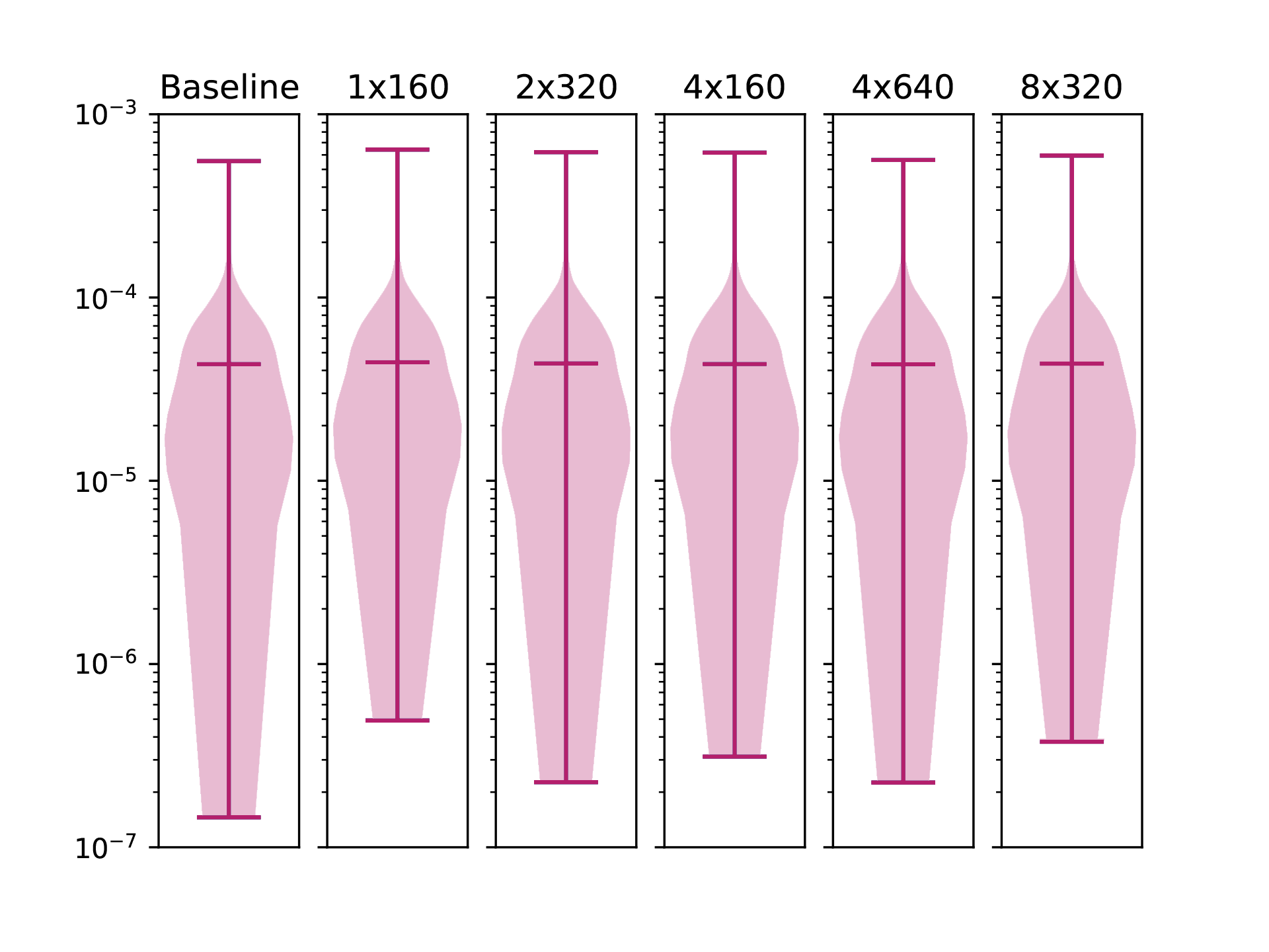
Figure 8: Violin plots comparing the mismatches (for the validation set) between the various baseline network architectures with the effect of the residual errors network. The middle horizontal line marks the median and the extent of the lines show the minimum and maximum values. In each panel, the envelope is proportional to the density of points. Above the plots the first number corresponds to the number of hidden layers while the second is the number of nodes in each hidden layer.

5 Exploration of Feature Space and Output Manipulation

5.1 Feature Space Manipulation

While working with the baseline network, we aimed for manipulations of the input space of the networks that would lead to a better mismatch. In some cases the input feature space dimension was increased and in some others the total size of the training dataset was increased by inserting an altered branch of samples.

a. Exploitation of similarities between waveforms. One such idea was to enlarge the input parameter space to four-dimensional, by adding a new parameter that describes physical relations between different waveforms. At 1.5 post-Newtonian (PN) order the time evolution of the frequency $f=\Omega/\pi$ (where $\Omega$ is the orbital frequency) of the quadrupolar part of the waveform is described by [113, 119]:

$$\frac{df}{dt}=\frac{96}{5}\pi^{8/3}\mathcal{M}_{c}+c^{5/3}f^{11/3}\left[1-\left(\frac{743}{336}+\frac{11\mu}{4M}\right)x+(4\pi-\beta)x^{3/2}+O(x^{2})\right],$$ (13)

where $M=m_{1}+m_{2}$ is the total mass of the binary system, $\mu=m_{1}m_{2}/M$ is the reduced mass, $\mathcal{M}_{c}=\mu^{3/5}M^{2/5}$ is the chirp mass and $x=(\pi Mf)^{2/3}$. At this order, the effect of the two spins $\chi_{1},\chi_{2}$ on the waveform, enters through a single parameter $\beta$, which is essentially a mass-ratio-weighted sum of the two spins:

$$\beta\equiv\left(\frac{113}{12}+\frac{25}{4q}\right)\frac{q^{2}}{(1+q)^{2}}\chi_{1}+\left(\frac{113}{12}+\frac{25q}{4}\right)\frac{1}{(1+q)^{2}}\chi_{2}.$$ (14)

Two different waveforms, characterized by different $\boldsymbol{\lambda}=\{q,\chi_{1},\chi_{2}\}$ values can thus have the same $\beta$ value, leading to identical waveforms at 1.5PN order (and rather similar waveforms, overall). So, the idea was to insert this new parameter, which has physical meaning, in order to help the network learn the interpolation coefficients.

b. Augmentation of the training set. Next, we tried to improve the problem of the presence of the worst mismatches at boundary values of the mass ratio and spins. As a remedy for the large mismatch when $q=1$ was approached, we first tried to augment the dataset with additional input samples $1/q,\chi_{2},\chi_{1}$. corresponding the same coefficients with $q,\chi_{1},\chi_{2}$, which, however, did not yield significant improvement. Next, we tried $\log(q)$ and $-\log(q)$ in place of $1/q$, which gave better results.

c. Dissection of the input space. Another tactic that was followed was that of dissecting the input feature space into a number of $K$ groups and evaluating the performance of the networks in each group. To that end, the input was divided to $K=2$ groups according to the value of the mass ratio $q$ and two separate networks were trained for both cases of amplitude and phase, each followed by its corresponding residual errors network. The hope was that the individual networks would produce smaller mismatches, by focusing on a smaller range of $q$, specifically $q\in[1,4.2]$ for the first group and $q\in[3.8,8]$ for the second group. Note that the $q$ ranges have a small overlap.

Table 9: Mean square error (MSE) of the predictions of different variants of the ANN surrogate model for the amplitude of the validation set, without (middle column) and with the addition of a network that models the residual error (right column). The smallest mismatch is shown in boldface. See the main text for the explanation of the different variants.

	MSE (average of 5 runs)	MSE (average of 5 runs)
	without residual network	with residual network
baseline	$1.84\times 10^{-7}\pm 1.90\times 10^{-10}$	$1.80\times 10^{-7}\pm 2.74\times 10^{-10}$
$\beta$ parameter	$1.82\times 10^{-7}\pm 2.44\times 10^{-10}$	$1.78\times 10^{-7}\pm 3.84\times 10^{-10}$
-$\log(q)$	$1.77\times 10^{-7}\pm 4.02\times 10^{-10}$	$1.77\times 10^{-7}\pm 3.17\times 10^{-10}$
K-networks	$1.86\times 10^{-7}\pm 1.25\times 10^{-10}$	${\bf 1.74\times 10^{-7}}\pm 8.03\times 10^{-11}$
Net per coef	${\bf 1.75\times 10^{-7}}\pm 2.26\times 10^{-10}$	$1.75\times 10^{-7}\pm 2.38\times 10^{-10}$
$f(1-\boldsymbol{y})$ output	$1.90\times 10^{-7}\pm 1.79\times 10^{-10}$	$1.82\times 10^{-7}\pm 5.47\times 10^{-10}$

5.2 Output Manipulation

a. Dedicated network per output coefficient. In an effort to achieve smaller mismatches by manipulating the output, we used a dedicated training network for each coefficient. For the baseline case examined in this work, we therefore used 18 networks for the amplitude and 8 networks for the phase. When the residuals were also modeled, an equal number of dedicated networks (one per residual) was also added.

b. Output augmentation. Finally, another idea to push the network to learn the desired output, was to insert a new branch with a function $f(\boldsymbol{y})$. For that reason, the quantity $(1-\boldsymbol{y})$ was added as an extra output for the training network. The final prediction $\hat{\boldsymbol{y}}$ was obtained by combining the predictions for $\boldsymbol{y}$ and $(1-\boldsymbol{y})$.

In all of the above cases, we also experimented with adding a network (or dedicated networks) for modeling the residual error. The results of our experiments are presented in the following Section.

Table 10: As in Table 9, but for the phase.

	MSE (average of 5 runs)	MSE (average of 5 runs)
	without residual network	with residual network
baseline	$1.08\times 10^{-8}\pm 2.11\times 10^{-10}$	$1.93\times 10^{-9}\pm 1.58\times 10^{-12}$
$\beta$ parameter	$9.97\times 10^{-9}\pm 8.59\times 10^{-11}$	$1.94\times 10^{-9}\pm 1.50\times 10^{-12}$
$-\log(q)$	$1.04\times 10^{-8}\pm 1.09\times 10^{-10}$	$2.35\times 10^{-9}\pm 5.89\times 10^{-11}$
$K$-networks	${\bf 4.47\times 10^{-9}}\pm 2.37\times 10^{-10}$	$2.94\times 10^{-9}\pm 8.51\times 10^{-11}$
Net per coef	$1.58\times 10^{-8}\pm 4.73\times 10^{-10}$	$1.96\times 10^{-9}\pm 1.72\times 10^{-11}$
$f(1-\boldsymbol{y})$ output	$1.37\times 10^{-8}\pm 3.40\times 10^{-10}$	${\bf 1.92\times 10^{-9}}\pm 1.22\times 10^{-12}$

Table 11: Mismatch $\mathcal{M}$ of the predictions of different variants of the ANN surrogate model (average of 5 runs). For each variant, the maximum, $95^{\text{th }}$ percentile and median mismatches are shown, with the addition of a network that models the residual errors as well as without it. The smallest mismatch is shown in boldface.

	Residual	Mismatch $\mathcal{M}$ (average of 5 runs)
	network	Max	$95^{\rm th}$ percentile	Median
baseline	No	$7.73\times 10^{-3}\pm 5.38\times 10^{-4}$	$2.95\times 10^{-4}\pm 6.61\times 10^{-6}$	$8.39\times 10^{-5}\pm 1.91\times 10^{-6}$
	Yes	$5.75\times 10^{-4}\pm 1.14\times 10^{-5}$	$1.33\times 10^{-4}\pm 1.01\times 10^{-7}$	${\bf 4.33\times 10^{-5}}\pm 2.73\times 10^{-8}$
$\beta$ parameter	No	$6.25\times 10^{-3}\pm 5.17\times 10^{-4}$	$2.68\times 10^{-4}\pm 6.72\times 10^{-6}$	$7.80\times 10^{-5}\pm 1.26\times 10^{-6}$
	Yes	$5.65\times 10^{-3}\pm 8.76\times 10^{-6}$	${\bf 1.32\times 10^{-4}}\pm 2.91\times 10^{-7}$	$4.33\times 10^{-5}\pm 7.02\times 10^{-8}$
$-\log(q)$	No	$5.57\times 10^{-3}\pm 3.28\times 10^{-4}$	$2.41\times 10^{-4}\pm 2.45\times 10^{-6}$	$7.10\times 10^{-5}\pm 3.00\times 10^{-6}$
	Yes	${\bf 5.62\times 10^{-4}}\pm 6.17\times 10^{-5}$	$1.42\times 10^{-4}\pm 3.24\times 10^{-6}$	$4.58\times 10^{-5}\pm 4.40\times 10^{-7}$
$K$-nets	No	$2.12\times 10^{-3}\pm 1.24\times 10^{-4}$	$1.67\times 10^{-4}\pm 2.18\times 10^{-6}$	$5.25\times 10^{-5}\pm 8.34\times 10^{-7}$
	Yes	$1.12\times 10^{-3}\pm 1.15\times 10^{-4}$	$1.49\times 10^{-4}\pm 6.37\times 10^{-7}$	$4.68\times 10^{-5}\pm 3.37\times 10^{-7}$
Net per coef	No	$5.50\times 10^{-2}\pm 2.33\times 10^{-2}$	$1.43\times 10^{-3}\pm 4.63\times 10^{-4}$	$1.89\times 10^{-4}\pm 2.55\times 10^{-5}$
	Yes	$7.32\times 10^{-4}\pm 1.60\times 10^{-4}$	$1.38\times 10^{-4}\pm 5.43\times 10^{-6}$	$4.43\times 10^{-5}\pm 6.83\times 10^{-7}$
$1-\boldsymbol{y}$	No	$6.67\times 10^{-3}\pm 1.16\times 10^{-3}$	$2.95\times 10^{-4}\pm 7.45\times 10^{-6}$	$8.51\times 10^{-5}\pm 1.66\times 10^{-6}$
	Yes	$5.80\times 10^{-4}\pm 1.37\times 10^{-5}$	${\bf 1.32\times 10^{-4}}\pm 1.55\times 10^{-7}$	${\bf 4.33\times 10^{-5}}\pm 5.40\times 10^{-8}$

6 Performance of different variants of the ANN surrogate model

Table 9 shows the MSE of the predictions of the different variants of the ANN surrogate model discussed in Sec. 5 for the amplitude of the validation set. Without a residual network, the variants with the $\beta$ parameter, the $1/q$ and $-\log(q)$ input augmentations and the individual networks per coefficient show a slight improvement in the mismatch. The variants with the dissection into $K=2$ networks and the output augmentation show a slight worsening, instead. Adding a network that models the residual error slightly improves or does not affect the MSE, except for the case of the $1/q$ input augmentation, where the MSE becomes slightly worse. Out of all variants shown in Table 9, the dissection into $K=2$ networks with residual error modeling shows the smallest MSE, which is $\sim 5\%$ ($\sim 3\%$) smaller than the MSE of the baseline network without (with) residual modeling. It is important to note that our method is compatible and thus can be used on top of any ANN architecture. Moreover, our experimental study has demonstrated notable enhancements when compared to the baseline model proposed by [100] which served as the starting point of our experimentation.

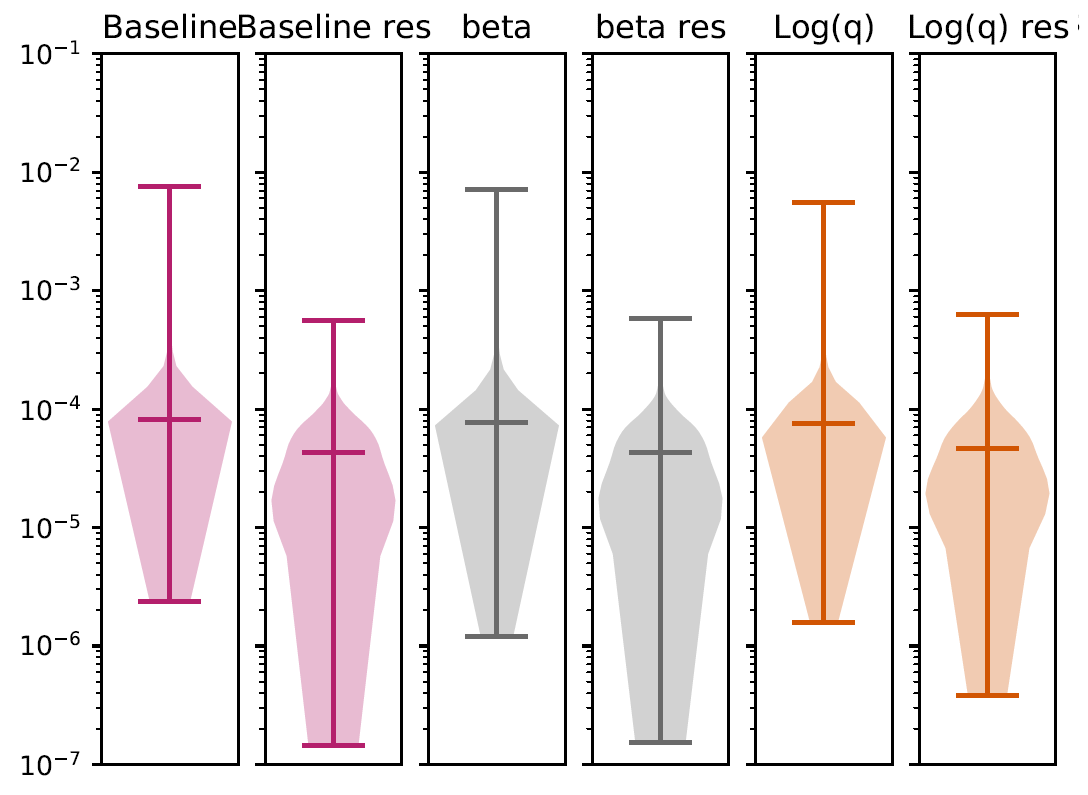
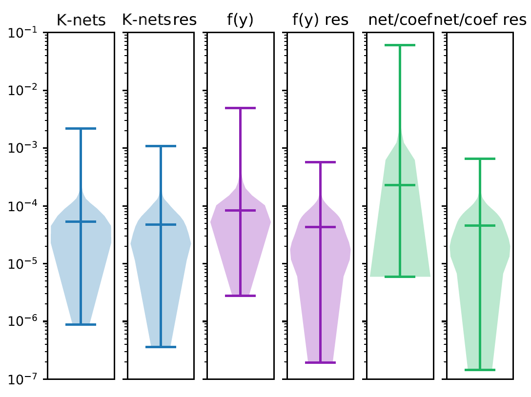
Figure 9: Violin plots comparing the mismatches for different variants of the ANN surrogate model without (left panel for each variant) and with the addition of a network that models the residual error (right panel for each variant).The middle horizontal line marks the median and the extent of the lines show the minimum and maximum values. In each panel, the envelope is proportional to the density of points. A significant reduction of the mismatch is achieved in several variants. See text for details.

Table 10 shows the corresponding MSE for the phase. Without a residual network, the variants with the $q$ input, the $\beta$ parameter, the $-\log(q)$ input augmentation and the dissection into $K=2$ networks show improvements between $\sim 4\%$ and $\sim 60\%$, whereas the remaining variants show a worsening of the MSE. When a network that models the residual error is added, the MSE is reduced significantly for all variants. The highest reduction, by a factor of $\sim 7$, can be observed for the output augmentation. This is the best case out of all variants shown in Table 10, with the baseline network with added residual error modeling coming a close second.

In Table 11 we show the mismatch $\mathcal{M}$ of the predictions of the different variants of the ANN surrogate model discussed in Sec. 5 (the average of 5 runs is shown). For each variant, the maximum, $95^{\text{th }}$ percentile and median mismatches are shown, both with and without the addition of a network that models the residual errors. The corresponding violin plots are shown in Fig. 9 (except for the case of $q$ input). For each variant (shown in different colors) the left (right) panel displays the case without (with) a network for the residual error. The middle horizontal line marks the median and the extent of the lines show the minimum and maximum values. The envelope is proportional to the density of points.

From the mismatch results displayed in Table 11 and in Fig. 9, it is evident that the most significant improvements to the ANN surrogate model come from the inclusion of the network that models the residual error. Both the minimum and maximum error are reduced by more than an order of magnitude, compared to the baseline network without residual error modeling. Specifically, the maximum error is reduced by a factor of $\sim 17$ for the variant with $q$ input and residual error modeling, compared to the baseline network. The minimum error is reduced by a factor of $\sim 15$ for the baseline with residual error modeling and by a similar factor for the dedicated networks per coefficient, compared to the baseline network without residual error modeling. The $95^{\text{th }}$ percentile mismatch is reduced by a factor of $\sim 2$ with respect to the baseline network without residual error modeling. The smallest $95^{\text{th }}$ percentile mismatches were achieved in the cases of the $\beta$ parameter and of the output augmentation, with the baseline model and the variant with $q$ input coming close second (all cases with residual error modeling added). The best performance of the median mismatch was observed for the baseline network with residual error modeling and for the variants with $q$ input and output augmentation (also with residual error modeling). Compared to the baseline network without residual error modeling, these variants had a median error reduced by a factor of $\sim 2$.

7 Discussion & Conclusions

Deep learning methods have been employed in gravitational-wave astronomy to accelerate the construction of surrogate waveforms for the inspiral of spin-aligned black hole binaries, among other applications. As we demonstrated here, the residual error of an ANN that models the coefficients of the surrogate waveform expansion has sufficient structure to be learnable by a second network. This is especially true for the residual error of the surrogate model coefficients for the phase of the waveform. We added a second ANN (of the same architecture as the main network) and showed that the maximum mismatch for waveforms in a validation set was reduced by more than an order of magnitude.

Furthermore, we explored several other ideas for improving the accuracy of the surrogate model, such as the exploitation of similarities between waveforms, the augmentation of the training set, the dissection of the input space, using dedicated networks per output coefficient and output augmentation. In several cases, small improvements were observed, but the most significant improvement still came from the addition of a second network that models the residual error. Since the residual error for more general surrogate waveform models (when e.g. eccentricity of tidal effects are included) may also have a specific structure, one can expect our method to be applicable in such more general cases. The gain in accuracy may then lead to significant gains in computational time. We plan to investigate such cases in the future.

Specifically, in a series of extensive experiments, we showed that the proposed bag-of-tricks methods can improve the maximum mismatched between real and reconstructed waveforms by 1.2-1.4 times, using the $-\text{log}(q)$ or $\beta$ parameter method, and up to 3.6 times, using the K-nets method, compared to the mismatch achieved by using the baseline model at zero additional computational overhead during deployment. Furthermore, the proposed residual error modeling method can achieve up to 13.4 times improved mismatch at about two times the computational overhead compared to the baseline method. This result is especially noteworthy when taking into consideration the fact that using networks with larger capacity as the baseline coefficient predictors only increases the computational cost without providing proportionate - or any - improvement in terms of mismatch. This means that in order to reach mismatch values of over an order of magnitude lower than the baseline network, regardless of its capacity, a second model that learns the first’s residual errors is essential.

While our results demonstrate the effectiveness of the proposed method in accurately predicting waveforms, we also acknowledge certain limitations that could be addressed in future research. Specifically, our study required a substantial amount of training data and the number of parameters was relatively low-dimensional compared to the 7-dimensional space of the general case of merging black holes. To further enhance the proposed approach, we recommend future studies to explore residual error networks and utilize the proposed ‘bag-of-tricks’ method to improve network performance in cases where dense training sets are not available.

One can also hope to perhaps model the residual errors even further, e.g. by adding a third network to model the “residual of the residual”, if a clustering persists at the next level. This suggestion is in line with residual connection based architectures [120], where each such connection can be viewed as residual error learning from its input to its desired output, i.e., the error of the previous neural structure.

8 Acknowledgments

We are grateful to Theocharis Apostolatos for suggesting to use the relation for $\beta$ and Leila Haegel, Maria Haney, George Pappas, Vasilis Skliris and Vijay Varma for useful discussions and comments. The authors gratefully acknowledge the Italian Instituto Nazionale di Fisica Nucleare (INFN), the French Centre National de la Recherche Scientifique (CNRS) and the Netherlands Organization for Scientific Research, for the construction and operation of the Virgo detector and the creation and support of the EGO consortium and the COST network CA17137 “G2Net” for support. Panagiotis Iosif acknowledges support by the European Research Council (ERC) under the European Union’s Horizon 2020 research and innovation programme under grant agreement No. 759253.

9 Appendix

The different panels in Fig. 10 display the two-dimensional distributions of mismatch values larger than the $95^{th}$ percentile (for different values of the greedy tolerance) for the waveforms in the validation set, when reconstructed using the EIM reduced basis via Eq. (2). The distributions are different at very small values of the greedy tolerance, when compared to the distributions for higher values of the greedy tolerance.

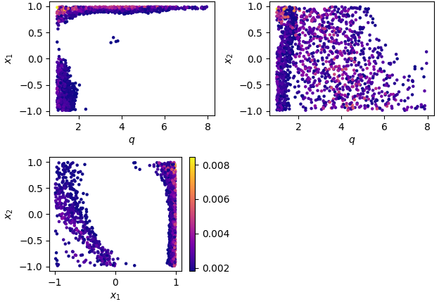
(a) tolerance $10^{-06}$

(b) tolerance $10^{-10}$

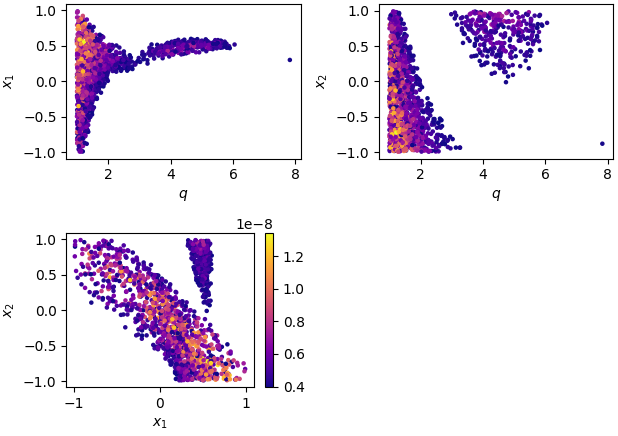
(c) tolerance $10^{-14}$

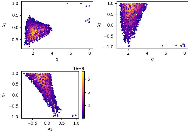
(d) tolerance $10^{-16}$

Figure 10: Two-dimensional and three-dimensional distribution of mismatch values larger than $\sim 8\times 10^{-5}$ ($95^{th}$ percentile) for the waveforms in the validartion set, when reconstructed using the EIM reduced basis via Eq. (2). The different panels correspond to different values of the greedy tolerance.

References

- [1] B. Abbott, et al., Observation of Gravitational Waves from a Binary Black Hole Merger, Phys. Rev. Lett. 116 (6) (2016) 061102. arXiv:1602.03837, doi:10.1103/PhysRevLett.116.061102.
- [2] J. Aasi, et al., Advanced LIGO, Class. Quant. Grav. 32 (2015) 074001. arXiv:1411.4547, doi:10.1088/0264-9381/32/7/074001.
- [3] B. Abbott, et al., GWTC-1: A Gravitational-Wave Transient Catalog of Compact Binary Mergers Observed by LIGO and Virgo during the First and Second Observing Runs, Phys. Rev. X 9 (3) (2019) 031040. arXiv:1811.12907, doi:10.1103/PhysRevX.9.031040.
- [4] F. Acernese, et al., Advanced Virgo: a second-generation interferometric gravitational wave detector, Classical and Quantum Gravity 32 (2) (2014) 024001. doi:10.1088/0264-9381/32/2/024001.
- [5] B. P. Abbott, et al., GW170817: Observation of Gravitational Waves from a Binary Neutron Star Inspiral, Phys. Rev. Lett. 119 (16) (2017) 161101. arXiv:1710.05832, doi:10.1103/PhysRevLett.119.161101.
-
[6]
B. P. Abbott, et al.,
Multi-messenger
observations of a binary neutron star merger, The Astrophysical Journal
848 (2) (2017) L12.
doi:10.3847/2041-8213/aa91c9.
URL http://dx.doi.org/10.3847/2041-8213/aa91c9 -
[7]
B. P. Abbott, et al.,
Gravitational waves and
gamma-rays from a binary neutron star merger: GW170817 and GRB 170817a,
ApJL 848 (2) (2017) L13.
doi:10.3847/2041-8213/aa920c.
URL https://doi.org/10.3847/2041-8213/aa920c - [8] R. Abbott, et al., GWTC-2: Compact Binary Coalescences Observed by LIGO and Virgo During the First Half of the Third Observing Run, Phys. Rev. X 11 (2021) 021053. doi:10.1103/PhysRevX.11.021053.
- [9] R. Abbott, et al., GWTC-3: Compact Binary Coalescences Observed by LIGO and Virgo During the Second Part of the Third Observing Run, arXiv e-prints (2021) arXiv:2111.03606arXiv:2111.03606.
- [10] B. P. Abbott, et al., Prospects for observing and localizing gravitational-wave transients with Advanced LIGO, Advanced Virgo and KAGRA, Living Reviews in Relativity 23 (1) (2020) 3. doi:10.1007/s41114-020-00026-9.
- [11] T. Akutsu, et al., KAGRA: 2.5 Generation Interferometric Gravitational Wave Detector, Nature Astronomy 3 (1) (2019) 35–40. doi:10.1038/s41550-018-0658-y.
-
[12]
T. Akutsu, et al., Overview of
KAGRA: Detector design and construction history, Progress of Theoretical
and Experimental Physics 2021 (5), 05A101 (08 2020).
doi:10.1093/ptep/ptaa125.
URL https://doi.org/10.1093/ptep/ptaa125 - [13] M. Saleem, et al., The science case for LIGO-India, Classical and Quantum Gravity 39 (2) (2022) 025004. arXiv:2105.01716, doi:10.1088/1361-6382/ac3b99.
- [14] M. Punturo, et al., The Einstein Telescope: a third-generation gravitational wave observatory, Class. Quantum Gravity 27 (19) (2010) 194002. doi:10.1088/0264-9381/27/19/194002.
- [15] M. Maggiore, et al., Science case for the Einstein telescope, Journal of Cosmology and Astroparticle Physics 2020 (3) (2020) 050. arXiv:1912.02622, doi:10.1088/1475-7516/2020/03/050.
- [16] D. Reitze, et al., Cosmic Explorer: The U.S. contribution to gravitational-wave astronomy beyond LIGO, in: Bull. Am. Astron. Soc., Vol. 51, 2019, p. 35. arXiv:1907.04833.
- [17] M. Evans, et al., A Horizon Study for Cosmic Explorer: Science, Observatories, and Community, arXiv e-prints (2021) arXiv:2109.09882arXiv:2109.09882.
- [18] B. P. Abbott, et al., Exploring the sensitivity of next generation gravitational wave detectors, Class. Quantum Gravity 34 (4) (2017) 044001. arXiv:1607.08697, doi:10.1088/1361-6382/aa51f4.
- [19] D. Reitze, M. Punturo, P. Couvares, S. Katsanevas, T. Kajita, V. Kalogera, H. Lueck, D. McClelland, S. Rowan, G. Sanders, B. S. Sathyaprakash, D. Shoemaker, J. van den Brand, Expanding the Reach of Gravitational Wave Astronomy to the Edge of the Universe: The Gravitational-Wave International Committee Study Reports on Next Generation Ground-based Gravitational-Wave Observatories, arXiv e-prints (2021) arXiv:2111.06986arXiv:2111.06986.
- [20] V. Kalogera, B. S. Sathyaprakash, M. Bailes, M.-A. Bizouard, et al., The Next Generation Global Gravitational Wave Observatory: The Science Book, arXiv e-prints (2021) arXiv:2111.06990arXiv:2111.06990.
-
[21]
L. Blanchet, Gravitational
radiation from post-newtonian sources and inspiralling compact binaries,
Living Reviews in Relativity 17 (1) (Feb 2014).
doi:10.12942/lrr-2014-2.
URL http://dx.doi.org/10.12942/lrr-2014-2 -
[22]
M. Campanelli, C. O. Lousto, P. Marronetti, Y. Zlochower,
Accurate
evolutions of orbiting black-hole binaries without excision, Phys. Rev.
Lett. 96 (2006) 111101.
doi:10.1103/PhysRevLett.96.111101.
URL https://link.aps.org/doi/10.1103/PhysRevLett.96.111101 -
[23]
F. Pretorius,
Evolution of
binary black-hole spacetimes, Phys. Rev. Lett. 95 (2005) 121101.
doi:10.1103/PhysRevLett.95.121101.
URL https://link.aps.org/doi/10.1103/PhysRevLett.95.121101 -
[24]
J. G. Baker, J. Centrella, D.-I. Choi, M. Koppitz, J. van Meter,
Gravitational-wave
extraction from an inspiraling configuration of merging black holes, Phys.
Rev. Lett. 96 (2006) 111102.
doi:10.1103/PhysRevLett.96.111102.
URL https://link.aps.org/doi/10.1103/PhysRevLett.96.111102 - [25] M. Boyle, D. Hemberger, D. A. B. Iozzo, G. Lovelace, S. Ossokine, H. P. Pfeiffer, M. A. Scheel, L. C. Stein, C. J. Woodford, A. B. Zimmerman, N. Afshari, K. Barkett, J. Blackman, K. Chatziioannou, T. Chu, N. Demos, N. Deppe, S. E. Field, N. L. Fischer, E. Foley, H. Fong, A. Garcia, M. Giesler, F. Hebert, I. Hinder, R. Katebi, H. Khan, L. E. Kidder, P. Kumar, K. Kuper, H. Lim, M. Okounkova, T. Ramirez, S. Rodriguez, H. R. Rüter, P. Schmidt, B. Szilagyi, S. A. Teukolsky, V. Varma, M. Walker, The SXS collaboration catalog of binary black hole simulations, Classical and Quantum Gravity 36 (19) (2019) 195006. arXiv:1904.04831, doi:10.1088/1361-6382/ab34e2.
- [26] T. Dietrich, D. Radice, S. Bernuzzi, F. Zappa, A. Perego, B. Brügmann, S. Vivekanandji Chaurasia, R. Dudi, W. Tichy, M. Ujevic, CoRe database of binary neutron star merger waveforms, Classical and Quantum Gravity 35 (24) (2018) 24LT01. arXiv:1806.01625, doi:10.1088/1361-6382/aaebc0.
- [27] A. Buonanno, Y. Pan, J. G. Baker, J. Centrella, B. J. Kelly, S. T. McWilliams, J. R. van Meter, Approaching faithful templates for nonspinning binary black holes using the effective-one-body approach, Phys. Rev. D 76 (10) (2007) 104049. arXiv:0706.3732, doi:10.1103/PhysRevD.76.104049.
- [28] A. Ramos-Buades, A. Buonanno, H. Estellés, M. Khalil, D. P. Mihaylov, S. Ossokine, L. Pompili, M. Shiferaw, SEOBNRv5PHM: Next generation of accurate and efficient multipolar precessing-spin effective-one-body waveforms for binary black holes, arXiv e-prints (2023) arXiv:2303.18046arXiv:2303.18046, doi:10.48550/arXiv.2303.18046.
- [29] T. Damour, A. Nagar, New effective-one-body description of coalescing nonprecessing spinning black-hole binaries, Phys. Rev. D 90 (4) (2014) 044018. arXiv:1406.6913, doi:10.1103/PhysRevD.90.044018.
-
[30]
R. Gamba, S. Akçay, S. Bernuzzi,
J. Williams,
Effective-one-body
waveforms for precessing coalescing compact binaries with post-newtonian
twist, Phys. Rev. D 106 (2022) 024020.
doi:10.1103/PhysRevD.106.024020.
URL https://link.aps.org/doi/10.1103/PhysRevD.106.024020 - [31] P. Ajith, S. Babak, Y. Chen, M. Hewitson, B. Krishnan, A. M. Sintes, J. T. Whelan, B. Brügmann, P. Diener, N. Dorband, J. Gonzalez, M. Hannam, S. Husa, D. Pollney, L. Rezzolla, L. Santamaría, U. Sperhake, J. Thornburg, Template bank for gravitational waveforms from coalescing binary black holes: Nonspinning binaries, Phys. Rev. D 77 (10) (2008) 104017. arXiv:0710.2335, doi:10.1103/PhysRevD.77.104017.
- [32] G. Pratten, C. García-Quirós, M. Colleoni, A. Ramos-Buades, H. Estellés, M. Mateu-Lucena, R. Jaume, M. Haney, D. Keitel, J. E. Thompson, S. Husa, Computationally efficient models for the dominant and subdominant harmonic modes of precessing binary black holes, Phys. Rev. D 103 (2021) 104056. doi:10.1103/PhysRevD.103.104056.
- [33] A. Buonanno, T. Damour, Effective one-body approach to general relativistic two-body dynamics, Phys. Rev. D 59 (8) (1999) 084006. arXiv:gr-qc/9811091, doi:10.1103/PhysRevD.59.084006.
- [34] H. Estellés, M. Colleoni, C. García-Quirós, S. Husa, D. Keitel, M. Mateu-Lucena, M. d. L. Planas, A. Ramos-Buades, New twists in compact binary waveform modeling: A fast time-domain model for precession, Phys. Rev. D 105 (8) (2022) 084040. arXiv:2105.05872, doi:10.1103/PhysRevD.105.084040.
- [35] T. Dietrich, S. Bernuzzi, W. Tichy, Closed-form tidal approximants for binary neutron star gravitational waveforms constructed from high-resolution numerical relativity simulations, Phys. Rev. D 96 (12) (2017) 121501. arXiv:1706.02969, doi:10.1103/PhysRevD.96.121501.
- [36] T. Dietrich, S. Khan, R. Dudi, S. J. Kapadia, P. Kumar, A. Nagar, F. Ohme, F. Pannarale, A. Samajdar, S. Bernuzzi, G. Carullo, W. Del Pozzo, M. Haney, C. Markakis, M. Pürrer, G. Riemenschneider, Y. E. Setyawati, K. W. Tsang, C. Van Den Broeck, Matter imprints in waveform models for neutron star binaries: Tidal and self-spin effects, Phys. Rev. D 99 (2) (2019) 024029. arXiv:1804.02235, doi:10.1103/PhysRevD.99.024029.
- [37] T. Dietrich, A. Samajdar, S. Khan, N. K. Johnson-McDaniel, R. Dudi, W. Tichy, Improving the NRTidal model for binary neutron star systems, Phys. Rev. D 100 (4) (2019) 044003. arXiv:1905.06011, doi:10.1103/PhysRevD.100.044003.
- [38] A. Matas, T. Dietrich, A. Buonanno, T. Hinderer, M. Pürrer, F. Foucart, M. Boyle, M. D. Duez, L. E. Kidder, H. P. Pfeiffer, M. A. Scheel, Aligned-spin neutron-star-black-hole waveform model based on the effective-one-body approach and numerical-relativity simulations, Phys. Rev. D 102 (4) (2020) 043023. arXiv:2004.10001, doi:10.1103/PhysRevD.102.043023.
- [39] J. E. Thompson, E. Fauchon-Jones, S. Khan, E. Nitoglia, F. Pannarale, T. Dietrich, M. Hannam, Modeling the gravitational wave signature of neutron star black hole coalescences, Phys. Rev. D 101 (12) (2020) 124059. arXiv:2002.08383, doi:10.1103/PhysRevD.101.124059.
-
[40]
T. Damour,
Coalescence of two
spinning black holes: An effective one-body approach, Phys. Rev. D 64 (2001)
124013.
doi:10.1103/PhysRevD.64.124013.
URL https://link.aps.org/doi/10.1103/PhysRevD.64.124013 -
[41]
T. Damour, P. Jaranowski, G. Schäfer,
Effective one body
approach to the dynamics of two spinning black holes with next-to-leading
order spin-orbit coupling, Phys. Rev. D 78 (2008) 024009.
doi:10.1103/PhysRevD.78.024009.
URL https://link.aps.org/doi/10.1103/PhysRevD.78.024009 - [42] Y. Pan, A. Buonanno, M. Boyle, L. T. Buchman, L. E. Kidder, H. P. Pfeiffer, M. A. Scheel, Inspiral-merger-ringdown multipolar waveforms of nonspinning black-hole binaries using the effective-one-body formalism, Phys. Rev. D 84 (12) (2011) 124052.
- [43] A. Taracchini, Y. Pan, A. Buonanno, E. Barausse, M. Boyle, T. Chu, G. Lovelace, H. P. Pfeiffer, M. A. Scheel, Prototype effective-one-body model for nonprecessing spinning inspiral-merger-ringdown waveforms, Phys. Rev. D 86 (2) (2012) 024011. arXiv:1202.0790, doi:10.1103/PhysRevD.86.024011.
- [44] Y. Pan, A. Buonanno, A. Taracchini, L. E. Kidder, A. H. Mroué, H. P. Pfeiffer, M. A. Scheel, B. Szilágyi, Inspiral-merger-ringdown waveforms of spinning, precessing black-hole binaries in the effective-one-body formalism, Phys. Rev. D 89 (8) (2014) 084006. arXiv:1307.6232, doi:10.1103/PhysRevD.89.084006.
- [45] A. Taracchini, A. Buonanno, Y. Pan, T. Hinderer, M. Boyle, D. A. Hemberger, L. E. Kidder, G. Lovelace, A. H. Mroué, H. P. Pfeiffer, M. A. Scheel, B. Szilágyi, N. W. Taylor, A. Zenginoglu, Effective-one-body model for black-hole binaries with generic mass ratios and spins, Phys. Rev. D 89 (6) (2014) 061502. arXiv:1311.2544, doi:10.1103/PhysRevD.89.061502.
- [46] A. Bohé, L. Shao, A. Taracchini, A. Buonanno, S. Babak, I. W. Harry, I. Hinder, S. Ossokine, M. Pürrer, V. Raymond, T. Chu, H. Fong, P. Kumar, H. P. Pfeiffer, M. Boyle, D. A. Hemberger, L. E. Kidder, G. Lovelace, M. A. Scheel, B. Szilágyi, Improved effective-one-body model of spinning, nonprecessing binary black holes for the era of gravitational-wave astrophysics with advanced detectors, Phys. Rev. D 95 (4) (2017) 044028. arXiv:1611.03703, doi:10.1103/PhysRevD.95.044028.
-
[47]
S. Babak, A. Taracchini, A. Buonanno,
Validating the
effective-one-body model of spinning, precessing binary black holes against
numerical relativity, Phys. Rev. D 95 (2017) 024010.
doi:10.1103/PhysRevD.95.024010.
URL https://link.aps.org/doi/10.1103/PhysRevD.95.024010 - [48] R. Cotesta, A. Buonanno, A. Bohé, A. Taracchini, I. Hinder, S. Ossokine, Enriching the symphony of gravitational waves from binary black holes by tuning higher harmonics, Phys. Rev. D 98 (8) (2018) 084028. arXiv:1803.10701, doi:10.1103/PhysRevD.98.084028.
- [49] S. Ossokine, A. Buonanno, S. Marsat, R. Cotesta, S. Babak, T. Dietrich, R. Haas, I. Hinder, H. P. Pfeiffer, M. Pürrer, C. J. Woodford, M. Boyle, L. E. Kidder, M. A. Scheel, B. Szilágyi, Multipolar effective-one-body waveforms for precessing binary black holes: Construction and validation, Phys. Rev. D 102 (4) (2020) 044055. arXiv:2004.09442, doi:10.1103/PhysRevD.102.044055.
- [50] R. Cotesta, S. Marsat, M. Pürrer, Frequency-domain reduced-order model of aligned-spin effective-one-body waveforms with higher-order modes, Phys. Rev. D 101 (12) (2020) 124040. arXiv:2003.12079, doi:10.1103/PhysRevD.101.124040.
- [51] L. Pompili, A. Buonanno, H. Estellés, M. Khalil, M. van de Meent, D. P. Mihaylov, S. Ossokine, M. Pürrer, A. Ramos-Buades, A. K. Mehta, R. Cotesta, S. Marsat, M. Boyle, L. E. Kidder, H. P. Pfeiffer, M. A. Scheel, H. R. Rüter, N. Vu, R. Dudi, S. Ma, K. Mitman, D. Melchor, S. Thomas, J. Sanchez, Laying the foundation of the effective-one-body waveform models SEOBNRv5: improved accuracy and efficiency for spinning non-precessing binary black holes, arXiv e-prints (2023) arXiv:2303.18039arXiv:2303.18039, doi:10.48550/arXiv.2303.18039.
- [52] M. van de Meent, A. Buonanno, D. P. Mihaylov, S. Ossokine, L. Pompili, N. Warburton, A. Pound, B. Wardell, L. Durkan, J. Miller, Enhancing the SEOBNRv5 effective-one-body waveform model with second-order gravitational self-force fluxes, arXiv e-prints (2023) arXiv:2303.18026arXiv:2303.18026, doi:10.48550/arXiv.2303.18026.
- [53] M. Khalil, A. Buonanno, H. Estellés, D. P. Mihaylov, S. Ossokine, L. Pompili, A. Ramos-Buades, Theoretical groundwork supporting the precessing-spin two-body dynamics of the effective-one-body waveform models SEOBNRv5, arXiv e-prints (2023) arXiv:2303.18143arXiv:2303.18143, doi:10.48550/arXiv.2303.18143.
-
[54]
P. Schmidt, M. Hannam, S. Husa,
Towards models of
gravitational waveforms from generic binaries: A simple approximate mapping
between precessing and nonprecessing inspiral signals, Phys. Rev. D 86
(2012) 104063.
doi:10.1103/PhysRevD.86.104063.
URL https://link.aps.org/doi/10.1103/PhysRevD.86.104063 -
[55]
M. Hannam, P. Schmidt, A. Bohé, L. Haegel, S. Husa, F. Ohme, G. Pratten,
M. Pürrer,
Simple model
of complete precessing black-hole-binary gravitational waveforms, Phys. Rev.
Lett. 113 (2014) 151101.
doi:10.1103/PhysRevLett.113.151101.
URL https://link.aps.org/doi/10.1103/PhysRevLett.113.151101 - [56] A. K. Mehta, C. K. Mishra, V. Varma, P. Ajith, Accurate inspiral-merger-ringdown gravitational waveforms for nonspinning black-hole binaries including the effect of subdominant modes, Phys. Rev. D 96 (12) (2017) 124010. arXiv:1708.03501, doi:10.1103/PhysRevD.96.124010.
- [57] L. London, S. Khan, E. Fauchon-Jones, C. García, M. Hannam, S. Husa, X. Jiménez-Forteza, C. Kalaghatgi, F. Ohme, F. Pannarale, First higher-multipole model of gravitational waves from spinning and coalescing black-hole binaries, Phys. Rev. Lett. 120 (16) (2018) 161102. arXiv:1708.00404, doi:10.1103/PhysRevLett.120.161102.
- [58] A. K. Mehta, P. Tiwari, N. K. Johnson-McDaniel, C. K. Mishra, V. Varma, P. Ajith, Including mode mixing in a higher-multipole model for gravitational waveforms from nonspinning black-hole binaries, Phys. Rev. D 100 (2) (2019) 024032. arXiv:1902.02731, doi:10.1103/PhysRevD.100.024032.
- [59] S. Khan, F. Ohme, K. Chatziioannou, M. Hannam, Including higher order multipoles in gravitational-wave models for precessing binary black holes, Phys. Rev. D 101 (2) (2020) 024056. arXiv:1911.06050, doi:10.1103/PhysRevD.101.024056.
- [60] G. Pratten, S. Husa, C. García-Quirós, M. Colleoni, A. Ramos-Buades, H. Estellés, R. Jaume, Setting the cornerstone for a family of models for gravitational waves from compact binaries: The dominant harmonic for nonprecessing quasicircular black holes, Phys. Rev. D 102 (6) (2020) 064001. arXiv:2001.11412, doi:10.1103/PhysRevD.102.064001.
- [61] C. García-Quirós, M. Colleoni, S. Husa, H. Estellés, G. Pratten, A. Ramos-Buades, M. Mateu-Lucena, R. Jaume, Multimode frequency-domain model for the gravitational wave signal from nonprecessing black-hole binaries, Phys. Rev. D 102 (6) (2020) 064002. arXiv:2001.10914, doi:10.1103/PhysRevD.102.064002.
- [62] H. Estellés, A. Ramos-Buades, S. Husa, C. García-Quirós, M. Colleoni, L. Haegel, R. Jaume, Phenomenological time domain model for dominant quadrupole gravitational wave signal of coalescing binary black holes, Phys. Rev. D 103 (12) (2021) 124060. arXiv:2004.08302, doi:10.1103/PhysRevD.103.124060.
- [63] C. García-Quirós, S. Husa, M. Mateu-Lucena, A. Borchers, Accelerating the evaluation of inspiral-merger-ringdown waveforms with adapted grids, Classical and Quantum Gravity 38 (1) (2021) 015006. arXiv:2001.10897, doi:10.1088/1361-6382/abc36e.
-
[64]
H. Estellés, S. Husa, M. Colleoni, D. Keitel, M. Mateu-Lucena,
C. García-Quirós, A. Ramos-Buades, A. Borchers,
Time-domain
phenomenological model of gravitational-wave subdominant harmonics for
quasicircular nonprecessing binary black hole coalescences, Phys. Rev. D 105
(2022) 084039.
doi:10.1103/PhysRevD.105.084039.
URL https://link.aps.org/doi/10.1103/PhysRevD.105.084039 - [65] S. Bernuzzi, A. Nagar, T. Dietrich, T. Damour, Modeling the Dynamics of Tidally Interacting Binary Neutron Stars up to the Merger, Phys. Rev. Lett. 114 (16) (2015) 161103. arXiv:1412.4553, doi:10.1103/PhysRevLett.114.161103.
- [66] A. Nagar, S. Bernuzzi, W. Del Pozzo, G. Riemenschneider, S. Akcay, G. Carullo, P. Fleig, S. Babak, K. W. Tsang, M. Colleoni, F. Messina, G. Pratten, D. Radice, P. Rettegno, M. Agathos, E. Fauchon-Jones, M. Hannam, S. Husa, T. Dietrich, P. Cerdá-Duran, J. A. Font, F. Pannarale, P. Schmidt, T. Damour, Time-domain effective-one-body gravitational waveforms for coalescing compact binaries with nonprecessing spins, tides, and self-spin effects, Phys. Rev. D 98 (10) (2018) 104052. arXiv:1806.01772, doi:10.1103/PhysRevD.98.104052.
- [67] A. Nagar, G. Pratten, G. Riemenschneider, R. Gamba, Multipolar effective one body model for nonspinning black hole binaries, Phys. Rev. D 101 (2) (2020) 024041. arXiv:1904.09550, doi:10.1103/PhysRevD.101.024041.
- [68] A. Nagar, G. Riemenschneider, G. Pratten, P. Rettegno, F. Messina, Multipolar effective one body waveform model for spin-aligned black hole binaries, Phys. Rev. D 102 (2) (2020) 024077. arXiv:2001.09082, doi:10.1103/PhysRevD.102.024077.
- [69] S. Akcay, R. Gamba, S. Bernuzzi, Hybrid post-Newtonian effective-one-body scheme for spin-precessing compact-binary waveforms up to merger, Phys. Rev. D 103 (2) (2021) 024014. arXiv:2005.05338, doi:10.1103/PhysRevD.103.024014.
- [70] Y. Setyawati, F. Ohme, Adding eccentricity to quasicircular binary-black-hole waveform models, Phys. Rev. D 103 (12) (2021) 124011. arXiv:2101.11033, doi:10.1103/PhysRevD.103.124011.
- [71] D. Chiaramello, A. Nagar, Faithful analytical effective-one-body waveform model for spin-aligned, moderately eccentric, coalescing black hole binaries, Phys. Rev. D 101 (10) (2020) 101501. arXiv:2001.11736, doi:10.1103/PhysRevD.101.101501.
- [72] A. Nagar, A. Bonino, P. Rettegno, Effective one-body multipolar waveform model for spin-aligned, quasicircular, eccentric, hyperbolic black hole binaries, Phys. Rev. D 103 (10) (2021) 104021. arXiv:2101.08624, doi:10.1103/PhysRevD.103.104021.
- [73] M. Khalil, A. Buonanno, J. Steinhoff, J. Vines, Radiation-reaction force and multipolar waveforms for eccentric, spin-aligned binaries in the effective-one-body formalism, Phys. Rev. D 104 (2) (2021) 024046. arXiv:2104.11705, doi:10.1103/PhysRevD.104.024046.
- [74] A. Ramos-Buades, A. Buonanno, M. Khalil, S. Ossokine, Effective-one-body multipolar waveforms for eccentric binary black holes with non-precessing spins, arXiv e-prints (2021) arXiv:2112.06952arXiv:2112.06952.
- [75] R. Abbott, et al., GW190412: Observation of a Binary-Black-Hole Coalescence with Asymmetric Masses, Phys. Rev. D 102 (4) (2020) 043015. arXiv:2004.08342, doi:10.1103/PhysRevD.102.043015.
- [76] R. Abbott, et al., GW190814: Gravitational Waves from the Coalescence of a 23 Solar Mass Black Hole with a 2.6 Solar Mass Compact Object, Astrophys. J. 896 (2) (2020) L44. arXiv:2006.12611, doi:10.3847/2041-8213/ab960f.
- [77] M. Colleoni, M. Mateu-Lucena, H. Estellés, C. García-Quirós, D. Keitel, G. Pratten, A. Ramos-Buades, S. Husa, Towards the routine use of subdominant harmonics in gravitational-wave inference: Reanalysis of GW190412 with generation X waveform models, Phys. Rev. D 103 (2) (2021) 024029. arXiv:2010.05830, doi:10.1103/PhysRevD.103.024029.
- [78] B. P. Abbott, et al., GW190425: Observation of a Compact Binary Coalescence with Total Mass 3.4 M⊙, ApJL 892 (1) (2020) L3. arXiv:2001.01761, doi:10.3847/2041-8213/ab75f5.
- [79] R. Abbott, et al., Observation of Gravitational Waves from Two Neutron Star-Black Hole Coalescences, ApJL 915 (1) (2021) L5. arXiv:2106.15163, doi:10.3847/2041-8213/ac082e.
- [80] R. Abbott, et al., GW190521: A Binary Black Hole Merger with a Total Mass of 150 M⊙, Phys. Rev. Lett. 125 (10) (2020) 101102. arXiv:2009.01075, doi:10.1103/PhysRevLett.125.101102.
- [81] H. Estellés, S. Husa, M. Colleoni, M. Mateu-Lucena, M. d. L. Planas, C. García-Quirós, D. Keitel, A. Ramos-Buades, A. K. Mehta, A. Buonanno, S. Ossokine, A Detailed Analysis of GW190521 with Phenomenological Waveform Models, ApJ 924 (2) (2022) 79. arXiv:2105.06360, doi:10.3847/1538-4357/ac33a0.
- [82] A. H. Nitz, C. D. Capano, GW190521 May Be an Intermediate-mass Ratio Inspiral, ApJL 907 (1) (2021) L9. arXiv:2010.12558, doi:10.3847/2041-8213/abccc5.
- [83] A. H. Nitz, S. Kumar, Y.-F. Wang, S. Kastha, S. Wu, M. Schäfer, R. Dhurkunde, C. D. Capano, 4-OGC: Catalog of gravitational waves from compact-binary mergers, arXiv e-prints (2021) arXiv:2112.06878arXiv:2112.06878.
- [84] A. Nagar, P. Rettegno, Efficient effective one body time-domain gravitational waveforms, Phys. Rev. D 99 (2) (2019) 021501. arXiv:1805.03891, doi:10.1103/PhysRevD.99.021501.
- [85] R. Gamba, S. Bernuzzi, A. Nagar, Fast, faithful, frequency-domain effective-one-body waveforms for compact binary coalescences, Phys. Rev. D 104 (8) (2021) 084058. arXiv:2012.00027, doi:10.1103/PhysRevD.104.084058.
- [86] G. Riemenschneider, P. Rettegno, M. Breschi, A. Albertini, R. Gamba, S. Bernuzzi, A. Nagar, Assessment of consistent next-to-quasicircular corrections and postadiabatic approximation in effective-one-body multipolar waveforms for binary black hole coalescences, Phys. Rev. D 104 (10) (2021) 104045. doi:10.1103/PhysRevD.104.104045.
- [87] D. P. Mihaylov, S. Ossokine, A. Buonanno, A. Ghosh, Fast post-adiabatic waveforms in the time domain: Applications to compact binary coalescences in LIGO and Virgo, Phys. Rev. D 104 (12) (2021) 124087. arXiv:2105.06983, doi:10.1103/PhysRevD.104.124087.
- [88] S. E. Field, C. R. Galley, J. S. Hesthaven, J. Kaye, M. Tiglio, Fast prediction and evaluation of gravitational waveforms using surrogate models, Physical Review X 4 (3) (2014) 031006.
- [89] M. Tiglio, A. Villanueva, Reduced Order and Surrogate Models for Gravitational Waves, arXiv e-prints (2021) arXiv:2101.11608arXiv:2101.11608.
- [90] J. Blackman, S. E. Field, C. R. Galley, B. Szilágyi, M. A. Scheel, M. Tiglio, D. A. Hemberger, Fast and Accurate Prediction of Numerical Relativity Waveforms from Binary Black Hole Coalescences Using Surrogate Models, Phys. Rev. Lett. 115 (12) (2015) 121102. arXiv:1502.07758, doi:10.1103/PhysRevLett.115.121102.
- [91] J. Blackman, S. E. Field, M. A. Scheel, C. R. Galley, D. A. Hemberger, P. Schmidt, R. Smith, A surrogate model of gravitational waveforms from numerical relativity simulations of precessing binary black hole mergers, Phys. Rev. D 95 (10) (2017) 104023.
- [92] J. Blackman, S. E. Field, M. A. Scheel, C. R. Galley, C. D. Ott, M. Boyle, L. E. Kidder, H. P. Pfeiffer, B. Szilágyi, Numerical relativity waveform surrogate model for generically precessing binary black hole mergers, Phys. Rev. D 96 (2) (2017) 024058. arXiv:1705.07089, doi:10.1103/PhysRevD.96.024058.
- [93] V. Varma, S. E. Field, M. A. Scheel, J. Blackman, L. E. Kidder, H. P. Pfeiffer, Surrogate model of hybridized numerical relativity binary black hole waveforms, Phys. Rev. D 99 (6) (2019) 064045. arXiv:1812.07865, doi:10.1103/PhysRevD.99.064045.
- [94] V. Varma, S. E. Field, M. A. Scheel, J. Blackman, D. Gerosa, L. C. Stein, L. E. Kidder, H. P. Pfeiffer, Surrogate models for precessing binary black hole simulations with unequal masses, Physical Review Research 1 (3) (2019) 033015. arXiv:1905.09300, doi:10.1103/PhysRevResearch.1.033015.
- [95] T. Islam, V. Varma, J. Lodman, S. E. Field, G. Khanna, M. A. Scheel, H. P. Pfeiffer, D. Gerosa, L. E. Kidder, Eccentric binary black hole surrogate models for the gravitational waveform and remnant properties: Comparable mass, nonspinning case, Phys. Rev. D 103 (6) (2021) 064022. arXiv:2101.11798, doi:10.1103/PhysRevD.103.064022.
- [96] M. Pürrer, Frequency domain reduced order model of aligned-spin effective-one-body waveforms with generic mass ratios and spins, Phys. Rev. D 93 (6) (2016) 064041. arXiv:1512.02248, doi:10.1103/PhysRevD.93.064041.
- [97] B. D. Lackey, S. Bernuzzi, C. R. Galley, J. Meidam, C. Van Den Broeck, Effective-one-body waveforms for binary neutron stars using surrogate models, Phys. Rev. D 95 (10) (2017) 104036. arXiv:1610.04742, doi:10.1103/PhysRevD.95.104036.
- [98] B. D. Lackey, M. Pürrer, A. Taracchini, S. Marsat, Surrogate model for an aligned-spin effective-one-body waveform model of binary neutron star inspirals using Gaussian process regression, Phys. Rev. D 100 (2) (2019) 024002. arXiv:1812.08643, doi:10.1103/PhysRevD.100.024002.
- [99] Q. Yun, W.-B. Han, X. Zhong, C. A. Benavides-Gallego, Surrogate model for gravitational waveforms of spin-aligned binary black holes with eccentricities, Phys. Rev. D 103 (12) (2021) 124053. arXiv:2104.03789, doi:10.1103/PhysRevD.103.124053.
- [100] S. Khan, R. Green, Gravitational-wave surrogate models powered by artificial neural networks, Phys. Rev. D 103 (6) (2021) 064015.
- [101] P. Nousi, S.-C. Fragkouli, N. Passalis, P. Iosif, T. Apostolatos, G. Pappas, N. Stergioulas, A. Tefas, Autoencoder-driven spiral representation learning for gravitational wave surrogate modelling (2021). arXiv:2107.04312.
- [102] E. Cuoco, J. Powell, M. Cavaglià, K. Ackley, M. Bejger, C. Chatterjee, M. Coughlin, S. Coughlin, P. Easter, R. Essick, H. Gabbard, T. Gebhard, S. Ghosh, L. Haegel, A. Iess, D. Keitel, Z. Márka, S. Márka, F. Morawski, T. Nguyen, R. Ormiston, M. Pürrer, M. Razzano, K. Staats, G. Vajente, D. Williams, Enhancing gravitational-wave science with machine learning, Machine Learning: Science and Technology 2 (1) (2020) 011002. doi:10.1088/2632-2153/abb93a.
- [103] D. Barsotti, F. Cerino, M. Tiglio, A. Villanueva, Gravitational wave surrogates through automated machine learning, arXiv e-prints (2021) arXiv:2110.08901arXiv:2110.08901.
- [104] A. J. Chua, C. R. Galley, M. Vallisneri, Reduced-order modeling with artificial neurons for gravitational-wave inference, Phys. Rev. Lett. 122 (21) (2019) 211101.
- [105] Y. Setyawati, M. Pürrer, F. Ohme, Regression methods in waveform modeling: a comparative study, Classical and Quantum Gravity 37 (7) (2020) 075012.
- [106] M. Tiglio, A. Villanueva, On ab initio-based, free and closed-form expressions for gravitational waves, Scientific Reports 11 (2021) 5832. doi:10.1038/s41598-021-85102-y.
-
[107]
D. Barsotti, F. Cerino, M. Tiglio, A. Villanueva,
Gravitational wave
surrogates through automated machine learning, Classical and Quantum Gravity
39 (8) (2022) 085011.
doi:10.1088/1361-6382/ac5ba1.
URL https://dx.doi.org/10.1088/1361-6382/ac5ba1 -
[108]
L. M. Thomas, G. Pratten, P. Schmidt,
Accelerating
multimodal gravitational waveforms from precessing compact binaries with
artificial neural networks, Phys. Rev. D 106 (2022) 104029.
doi:10.1103/PhysRevD.106.104029.
URL https://link.aps.org/doi/10.1103/PhysRevD.106.104029 - [109] M. Maggiore, Gravitational Waves Volume 1: Theory and Experiments, Oxford University Press, 2008. doi:10.1093/acprof:oso/9780198570745.001.0001.
-
[110]
A. Nitz, I. Harry, D. Brown, C. M. Biwer, J. Willis, T. D. Canton, C. Capano,
T. Dent, L. Pekowsky, A. R. Williamson, G. S. C. Davies, S. De, M. Cabero,
B. Machenschalk, P. Kumar, D. Macleod, S. Reyes, dfinstad, F. Pannarale,
T. Massinger, S. Kumar, M. Tápai, L. Singer, S. Khan, S. Fairhurst,
A. Nielsen, S. Singh, shasvath, B. U. V. Gadre, I. Dorrington,
gwastro/pycbc: Pycbc release
1.18.1 (May 2021).
doi:10.5281/zenodo.4849433.
URL https://doi.org/10.5281/zenodo.4849433 - [111] LIGO Scientific Collaboration, LIGO Algorithm Library - LALSuite, free software (GPL) (2018). doi:10.7935/GT1W-FZ16.
- [112] C. R. Galley, RomPy package, https://bitbucket.org/chadgalley/rompy/ (2020).
-
[113]
C. Cutler, E. E. Flanagan,
Gravitational waves from
merging compact binaries: How accurately can one extract the binary’s
parameters from the inspiral waveform?, Phys. Rev. D 49 (6) (1994)
2658–2697.
doi:10.1103/physrevd.49.2658.
URL http://dx.doi.org/10.1103/PhysRevD.49.2658 -
[114]
Ligo document t1800044-v5,
updated advanced ligo sensitivity design curve.
URL https://dcc.ligo.org/LIGO-T1800044/public - [115] D. P. Kingma, J. Ba, Adam: A method for stochastic optimization (2017). arXiv:1412.6980.
-
[116]
V. Nair, G. E. Hinton,
Rectified linear units
improve restricted boltzmann machines, in: ICML, 2010, pp. 807–814.
URL https://icml.cc/Conferences/2010/papers/432.pdf - [117] H. Zheng, Z. Yang, W. Liu, J. Liang, Y. Li, Improving deep neural networks using softplus units, 2015 International Joint Conference on Neural Networks (IJCNN) (2015) 1–4.
- [118] scikit learn, 6.3. preprocessing data, https://scikit-learn.org/stable/modules/preprocessing.html.
- [119] L. E. Kidder, C. M. Will, A. G. Wiseman, Spin effects in the inspiral of coalescing compact binaries, Phys. Rev. D 47 (10) (1993) R4183–R4187. arXiv:gr-qc/9211025, doi:10.1103/PhysRevD.47.R4183.
- [120] K. He, X. Zhang, S. Ren, J. Sun, Deep residual learning for image recognition, in: Proceedings of the IEEE conference on computer vision and pattern recognition, 2016, pp. 770–778.