FormNet: Structural Encoding beyond Sequential Modeling in
Form Document Information Extraction

Abstract

Sequence modeling has demonstrated state-of-the-art performance on natural language and document understanding tasks. However, it is challenging to correctly serialize tokens in form-like documents in practice due to their variety of layout patterns. We propose FormNet, a structure-aware sequence model to mitigate the suboptimal serialization of forms. First, we design Rich Attention that leverages the spatial relationship between tokens in a form for more precise attention score calculation. Second, we construct Super-Tokens for each word by embedding representations from their neighboring tokens through graph convolutions. FormNet therefore explicitly recovers local syntactic information that may have been lost during serialization. In experiments, FormNet outperforms existing methods with a more compact model size and less pre-training data, establishing new state-of-the-art performance on CORD, FUNSD and Payment benchmarks.

1 Introduction

Form-like document understanding is a surging research topic because of its practical applications in automating the process of extracting and organizing valuable text data sources such as marketing documents, advertisements and receipts.

Typical documents are represented using natural languages; understanding articles or web content Antonacopoulos et al. (2009); Luong et al. (2012); Soto and Yoo (2019) has been studied extensively. However, form-like documents often have more complex layouts that contain structured objects, such as tables and columns. Therefore, form documents have unique challenges compared to natural language documents stemming from their structural characteristics, and have been largely under-explored.

In this work, we study critical information extraction from form documents, which is the fundamental subtask of form document understanding. Following the success of sequence modeling in natural language understanding (NLU), a natural approach to tackle this problem is to first serialize the form documents and then apply state-of-the-art sequence models to them. For example, Palm et al. (2017) use Seq2seq Sutskever et al. (2014) with RNN, and  Hwang et al. (2019) use transformers Vaswani et al. (2017). However, interwoven columns, tables, and text blocks make serialization difficult, substantially limiting the performance of a strict serialization approach.

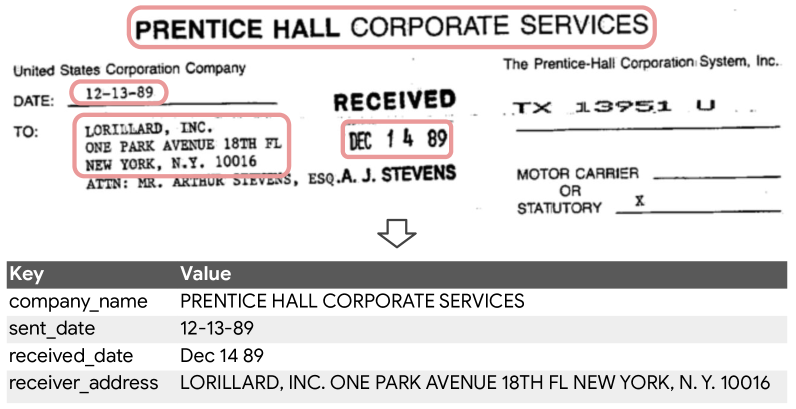
Figure 1: An illustration of the form document information extraction task.

To model the structural information present in documents, Katti et al. (2018); Zhao et al. (2019); Denk and Reisswig (2019) treat the documents as 2D image inputs and directly apply convolutional networks on them to preserve the spatial context during learning and inference. However, the performance is limited by the resolution of the 2D input grids. Another approach is a two-step pipeline  Hirano et al. (2007) that leverages computer vision algorithms to first infer the layout structures of forms and then perform sequence information extraction. The methods are mostly demonstrated on plain text articles or documents Yang et al. (2017); Soto and Yoo (2019) but not on highly entangled form documents Davis et al. (2019); Zhang et al. (2019).

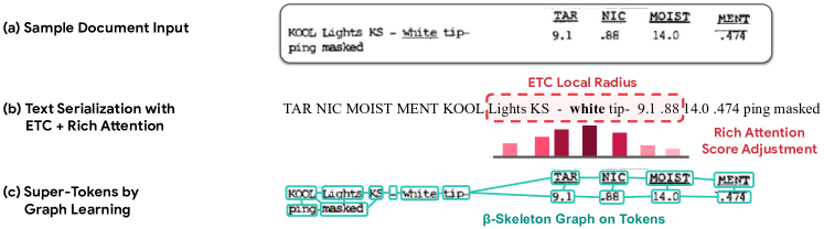
Figure 2: A walk-through example of the proposed Rich Attention and Super-Tokens of FormNet. (a) Input document. (b) The ETC transformer Ainslie et al. (2020) – the core of our system – is able to model long inputs by limiting attention to a local radius of serialized tokens. The proposed Rich Attention uses the spatial relationship between tokens to penalize unlikely attention edges. In this example, for the word ‘white’, Rich Attention increases the relative weight for spatially nearby tokens such as ‘KS’, ‘-’ and ‘tip’, while decreasing it for others, resulting in spatially aware attention scores. (c) Even though they belong to the same entity, KOOL and masked may not be visible to each other from within the local radius of ETC after the left-to-right, top-to-bottom serialization step, which breaks the text group on the left into multiple text segments. Our proposed Super-Tokens are generated by executing graph convolutional networks directly on 2D tokens before serialization. The edges of the graph leverage the inductive bias of the $\beta$-skeleton graph, allowing information propagation w.r.t. the structural layout of documents before text serialization introduces noise. Note that the $\beta$-skeleton graph connects KOOL and masked in this example.

In this work, we propose FormNet, a structure-aware sequence model to mitigate the suboptimal serialization of forms by bridging the gap between plain sequence models and grid-like convolutional models. Specifically, we first design Rich Attention, which leverages the spatial relationships between tokens in a form to calculate a more structurally meaningful attention score, and apply it in a recent transformer architecture for long documents Ainslie et al. (2020). Second, we construct Super-Tokens for each word in a form by embedding representations from their neighboring tokens through graph convolutions. The graph construction process leverages strong inductive biases about how tokens are related to one another spatially in forms. Essentially, given a form document, FormNet builds contextualized Super-Tokens before serialization errors can be propagated. A transformer model then takes these Super-Tokens as input to perform sequential entity tagging and extraction.

In our experiments, FormNet outperforms existing methods while using (1) smaller model sizes and (2) less pre-training data while (3) avoiding the need for vision features. In particular, FormNet achieves new best F1 scores on CORD and FUNSD (97.28% and 84.69%, respectively) while using a 64% sized model and 7.1x less pre-training data than the most recent DocFormer Appalaraju et al. (2021).

2 Related Work

Document information extraction was first studied in handcrafted rule-based models Lebourgeois et al. (1992); O’Gorman (1993); Ha et al. (1995); Simon et al. (1997). Later Marinai et al. (2005); Shilman et al. (2005); Wei et al. (2013); Chiticariu et al. (2013); Schuster et al. (2013) use learning-based approaches with engineered features. These methods encode low-level raw pixels  Marinai et al. (2005) or assume form templates are known a priori Chiticariu et al. (2013); Schuster et al. (2013), which limits their generalization to documents with specific layout structures.

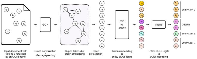
Figure 3: System overview of the proposed FormNet for form document key information extraction. Given a document, we first use the BERT-multilingual vocabulary to tokenize the extracted OCR words. We then feed the tokens and their corresponding 2D coordinates into a Graph Convolutional Network (GCN) for graph construction and message passing. Next, we use ETC Ainslie et al. (2020) transformers with the proposed Rich Attention (RichAtt) mechanism to process the GCN-encoded structure-aware Super-Tokens for schema learning. Finally, the Viterbi algorithm is used to decode and obtain the final entity extraction outputs.

In addition to models with limited or no learning capabilities, neural models have also been studied. Palm et al. (2017); Aggarwal et al. (2020) use an RNN for document information extraction, while Katti et al. (2018); Zhao et al. (2019); Denk and Reisswig (2019) investigate convolutional models. There are also self-attention networks (transformers) for document information extraction, motivated by their success in conventional NLU tasks. Majumder et al. (2020) extend BERT to representation learning for form documents. Garncarek et al. (2020) modified the attention mechanism in RoBERTa Liu et al. (2019b). Xu et al. (2020, 2021); Powalski et al. (2021); Appalaraju et al. (2021) are multimodal models that combine BERT-like architectures Devlin et al. (2019) and advanced computer vision models to extract visual content in images. Similarly, SPADE Hwang et al. (2021) is a graph decoder built upon the transformer models for better structure prediction compared to simple BIO tagging. The proposed FormNet is orthogonal to multimodal transformers and SPADE. Compared with multimodal models, FormNet focuses on modeling relations between words through graph convolutional learning as well as Rich Attention without using any visual modality; compared with SPADE, FormNet uses a graph encoder to encode inductive biases in form input. A straightforward extension would be to combine FormNet with either layout transformers or SPADE for capturing visual cues or better decoding, which we leave for future work.

Graph learning with sequence models has also been studied. On top of the encoded information through graph learning, Qian et al. (2019); Liu et al. (2019a); Yu et al. (2020) use RNN and CRF while we study Rich Attention in FormNet for decoding. Peng et al. (2017); Song et al. (2018) do not study document information extraction.

3 FormNet for Information Extraction

Problem Formulation.

Given serialized words of a form document, we formulate the problem as sequential tagging for tokenized words by predicting the corresponding key entity classes for each token. Specifically, we use the “BIOES” scheme – $\>\{$Begin, Inside, Outside, End, Single$\}$ Ratinov and Roth (2009) to mark the spans of entities in token sequences and then apply the Viterbi algorithm.

Proposed Approach.

By treating the problem as a sequential tagging task after serialization, we can adopt any sequence model. To handle potentially long documents (e.g. multi-page documents), we select the long-sequence transformer extension ETC Ainslie et al. (2020) as our backbone.

In practice, it is common to see an entity sequence cross multiple spans of a form document, demonstrating the difficulty of recovering from serialization errors. As illustrated in Figure 2(b), 9.1 is next to tip-, while ping masked belong to the same entity as tip- are distant from it under the imperfect serialization. Our remedy is to encode the original 2D structural patterns of forms in addition to positions within the serialized sentences. We propose two novel components to enhance ETC: Rich Attention and Super-Tokens (Figure 2). Rich Attention captures not only the semantic relationship but also the spatial distance between every pair of tokens in ETC’s attention component. Super-tokens are constructed by graph convolutional networks before being fed into ETC. They model local relationships between pairs of tokens that might not be visible to each other or correctly inferred in an ETC model after suboptimal serialization.

Figure 3 shows the overall system pipeline. We discuss the details of ETC in Sec. 3.1, Rich Attention in Sec. 3.2, and Super-Token in Sec. 3.3.

3.1 Extended Transformer Construction

Transformers Vaswani et al. (2017) have demonstrated state-of-the-art performance on sequence modeling compared with RNNs. Extended Transformer Construction (ETC; Ainslie et al., 2020) further scales transformers to long sequences by replacing standard (quadratic complexity) attention with a sparse global-local attention mechanism. The small number of “dummy” global tokens attend to all input tokens, but the input tokens attend only locally to other input tokens within a specified local radius. An example can be found in Figure 2(b). As a result, space and time complexity are linear in the long input length for a fixed local radius and global input length. Furthermore, ETC allows a specialized implementation for efficient computation under this design. We refer interested readers to Ainslie et al. (2020) for more details. In this work, we adopt ETC with a single global token as the backbone, as its linear complexity of attention with efficient implementation is critical to long document modeling in practice (e.g. thousands of tokens per document).

A key component in transformers for sequence modeling is the positional encoding Vaswani et al. (2017), which models the positional information of each token in the sequence. Similarly, the original implementation of ETC uses Shaw et al. (2018) for (relative) positional encoding. However, token offsets measured based on the error-prone serialization may limit the power of positional encoding. We address this inadequacy by proposing Rich Attention as an alternative, discussed in Section 3.2.

3.2 Rich Attention

Approach.

Our new architecture – inspired by work in dependency parsing (Dozat, 2019), and which we call Rich Attention – avoids the deficiencies of absolute and relative embeddings Shaw et al. (2018) by avoiding embeddings entirely. Instead, we compute the order of and log distance between pairs of tokens with respect to the x and y axis on the layout grid, and adjust the pre-softmax attention scores of each pair as a direct function of these values. At a high level, for each attention head at each layer $\ell$, the model examines each pair of token representations $\mathbf{h}^{\ell}_{i},\mathbf{h}^{\ell}_{j}$, whose actual order (using curly Iverson brackets) and log-distance are

$$o_{ij}=\{i<j\}\mbox{ and }d_{ij}=\ln(1+|i-j|).$$

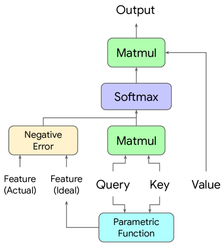
Figure 4: The network uses the Query and Key vectors to consider what value some low-level feature (e.g. distance) should take if the tokens are related, and penalizes the attention score based on the error.

The model then determines the “ideal” orders and distances the tokens should have if there is a meaningful relationship between them.

$$p_{ij} =\texttt{Sigmoid}(\text{affine}^{(p)}([\mathbf{h}^{\ell}_{i};\mathbf{h}^{\ell}_{j}]))$$ (1)

$$\mu_{ij} =\text{affine}^{(\mu)}([\mathbf{h}^{\ell}_{i};\mathbf{h}^{\ell}_{j}])$$ (2)

It compare the prediction and groudtruth using sigmoid cross-entropy and $L_{2}$ losses:

$$s^{(o)}_{ij} =o_{ij}\ln(p_{ij})+(1-o_{ij})\ln(1-p_{ij})$$ (3)

$$s^{(d)}_{ij} =-\frac{\theta^{2}(d_{ij}-\mu_{ij})^{2}}{2}$$ (4)

Finally, these are added to the usual attention score

$$s_{ij}=\mathbf{q}_{i}^{\top}\mathbf{k}_{j}+s_{ij}^{(o)}+s_{ij}^{(d)},$$

Figure 5: A high-level visualization of how rich attention might act on a sentence within a head that composes words with their syntactic modifiers. There are three adjectives that the word crow might attend to. However, one of them (lazy) is on the wrong side, so its attention edge is penalized. Another (sly) is many tokens away, so its attention edge is also penalized. Only one (cunning) receives no significant penalties.

where $\mathbf{q}_{i}=\text{affine}^{(q)}(\mathbf{h}_{i})$ and $\mathbf{k}_{j}=\text{affine}^{(k)}(\mathbf{h}_{j})$. The rich attention pipeline is shown in Figure 4. By penalizing attention edges for violating these soft order/distance constraints, we essentially build into the model the ability to learn logical implication rules such as “if $x_{i}$ is a noun, and $x_{j}$ is an adjective, and $x_{i}$ is related (i.e. attends) to $x_{j}$, then $x_{j}$ is to the left of $x_{i}$”. Note the unidirectionality of this rule – there could be many unrelated adjectives to the left of $x_{i}$, so the converse (which this approach cannot learn) does not hold in any general sense. This is shown graphically in Figure 5.

Justification. The approach taken here is not arbitrary. It can be derived algebraically from the probability mass/density functions of the distributions we assume for each feature, and the assumption that a query’s attention vector represents a probability distribution. Traditional dot product attention and relative position biases (Raffel et al., 2020) can likewise be derived from this method, providing incidental justification for the approach. Consider the following, letting $L(X)=\ln(P(X))$ for brevity:

$$P(a_{ij}\mid\mathbf{h}_{i},\mathbf{h}_{j}) =\frac{P(\mathbf{h}_{i},\mathbf{h}_{j}\mid a_{ij})P(a_{ij})}{\sum\limits_{j^{\prime}}\left[P(\mathbf{h}_{i},\mathbf{h}_{j^{\prime}}\mid a_{ij^{\prime}})P(a_{ij^{\prime}})\right]}$$

$$=\frac{\exp\left(L(\mathbf{h}_{i},\mathbf{h}_{j}\mid a_{ij})+L(a_{ij})\right)}{\sum\limits_{j^{\prime}}\exp\left(L(\mathbf{h}_{i},\mathbf{h}_{j^{\prime}}\mid a_{ij^{\prime}})+L(a_{ij^{\prime}})\right)}$$

$$=\text{soft}\max_{j^{\prime}}\left(L(\mathbf{h}_{i},\mathbf{h}_{j^{\prime}}\mid a_{ij^{\prime}})+L(a_{ij^{\prime}})\right)_{j}$$ (5)

Here $\mathbf{a}_{i}$ represents a latent categorical “attention” variable. Eq. (5) shows that the softmax function itself can actually be derived from posterior probabilities, by simply applying Bayes’ rule and then observing that $x=\exp(\ln(x))$ That is, one need not define the posterior as being the softmax of some expression, it simply is the softmax of some expression, specifically one that falls out of the assumptions one makes (explicitly or implicitly).

When we plug the Gaussian probability density function into $L(\mathbf{h}_{i},\mathbf{h}_{j}\mid a_{ij})$, the expression simplifies to dot-product attention (with one additional fancy bias term); we show this in Appendix C. If we assume $L(a_{ij})$ is uniform, then it divides out of the softmax and we can ignore it. If we assume it follows a Bernoulli distribution – such that $L(a_{ij}=1;p_{ij})=\ln(p_{ij})$ – it becomes equivalent to a learned bias matrix $B$.

Now, if we assume there is another feature $f_{ij}$ that conditions the presence of attention, such as the order or distance of $i$ and $j$, then we can use the same method to derive a parametric expression describing its impact on the attention probability.

$$P(a_{ij}\mid f_{ij},\mathbf{h}_{i},\mathbf{h}_{j})=\text{soft}\max_{j^{\prime}}($$

$$\qquad L(f_{ij^{\prime}}\mid\mathbf{h}_{i},\mathbf{h}_{j^{\prime}},a_{ij^{\prime}})+L(\mathbf{h}_{i},\mathbf{h}_{j^{\prime}}\mid a_{ij^{\prime}})+L(a_{ij^{\prime}}))_{j}$$

The new term can be expanded by explicating assumptions about the distributions that govern $P(f_{ij}\mid\mathbf{h}_{i},\mathbf{h}_{j},a_{ij})$ and simplifying the expression that results from substituting their probability functions. If $f_{ij}$ is binary, then this process yields Eq. (3), and if $\ln(f_{ij})$ is normally distributed, we reach Eq. (4), as derived in Appendix C. Given multiple conditionally independent features – such as the order and distance – their individual scores can be calculated in this way and summed. Furthermore, relative position biases (Raffel et al., 2020) can thus be understood in this framework as binary features (e.g. $f_{ij}=\{i-j=-2\}$) that are conditionally independent of $\mathbf{h}_{i}$, $\mathbf{h}_{j}$ given $a_{ij}$, meaning that $L(f_{ij}\mid\mathbf{h}_{i},\mathbf{h}_{j},a_{ij})=L(f_{ij}\mid a_{ij})$.

We call this new attention paradigm Rich Attention because it allows the attention mechanism to be enriched with an arbitrary set of low-level features. We use it to add order/distance features with respect to the x and y axes of a grid – but it can also be used in a standard text transformer to encode order/distance/segment information, or it could be used in an image transformer (Parmar et al., 2018) to encode relative pixel angle/distance information, without resorting to lossy quantization and finite embedding tables.

3.3 Super-Token by Graph Learning

The key to sparsifying attention mechanisms in ETC Ainslie et al. (2020) for long sequence modeling is to have every token only attend to tokens that are within a pre-specified local radius in the serialized sequence. The main drawback to ETC in form understanding is that imperfect serialization sometimes results in entities being serialized too far apart from each other to attend in the local-local attention component (i.e. outside the local radius). A naive solution is to increase the local radius in ETC. However, it sacrifices the efficiency for modeling long sequences. Also, the self-attention may not be able to fully identify relevant tokens when there are many distractors (Figure 9; Serrano and Smith, 2019).

To alleviate the issue, we construct a graph to connect nearby tokens in a form document. We design the edges of the graph based on strong inductive biases so that they have higher probabilities of belonging to the same entity type (Figure 2(c) and 6). Then, for each token, we obtain its Super-Token embedding by applying graph convolutions along these edges to aggregate semantically meaningful information from its neighboring tokens. We use these super-tokens as input to the Rich Attention ETC for sequential tagging. This means that even though an entity may have been broken up into multiple segments due to poor serialization, the super-tokens learned by the graph convolutional network will have recovered much of the context of the entity phrase. We next introduce graph construction and the learning algorithm.

Node Definition.

Given a document with $N$ tokens denoted by $T=\{t_{1},t_{2},\ldots t_{N}\}$, we let $t_{k}$ refer to the $k$-th token in a text sequence returned by the OCR engine. The OCR engine generates the bounding box sizes and locations for all tokens, as well as the text within each box. We define node input representation for all tokens $T$ as vertices $V=\{\mathbf{v}_{1},\mathbf{v}_{2},\ldots\mathbf{v}_{N}\}$, where $\mathbf{v}_{k}$ concatenates attributes available for $t_{k}$. In our design, we use three common input modalities: (a) one-hot word embeddings, (b) spatial embeddings from the normalized Cartesian coordinate values of the four corners and height and width of a token bounding box Qian et al. (2019); Davis et al. (2019); Liu et al. (2019a). The benefit of representing tokens in this way is that one can add more attributes to a vertex by simple concatenation without changing the macro graph architecture.

Edge Definition.

While the vertices $V$ represent tokens in a document, the edges characterize the relationship between all pairs of vertices. Precisely, we define directed edge embeddings for a set of edges $E$, where each edge $\mathbf{e}_{kl}$ connects two vertices $\mathbf{v}_{k}$ and $\mathbf{v}_{l}$, concatenating quantitative edge attributes. In our design, the edge embedding is composed of the relative distance between the centers, top left corners, and bottom right corners of the token bounding boxes. The embedding also contains the shortest distances between the bounding boxes along the horizontal and vertical axis. Finally, we include the height and width aspect ratio of $\mathbf{v}_{k}$, $\mathbf{v}_{l}$, and the bounding box that covers both of them.

Graph construction.

After contructing edge embeddings, we need discrete graphs to define connectivities. One approach would be to create k-Nearest-Neighbors graphs Zhang et al. (2020) – but these may contain isolated components, which is not ideal for information propagation. Instead, we construct graphs using the $\beta$-skeleton algorithm Kirkpatrick and Radke (1985) with $\beta=1$, which is found useful for document understanding in Wang et al. (2022); Lee et al. (2021). It essentially creates a “ball-of-sight” graph with a linearly-bounded number of edges while also guaranteeing global connectivity as shown in Figure 6. More examples of constructed $\beta$-skeleton graphs can be found in Figure 11 in the Appendix.

Message passing.

Graph message-passing is the key to propagating representations along the edges defined by the inductive bias, $\beta$-skeleton, that are free from the left-to-right top-to-bottom form document serialization. In our design, we perform graph convolutions (GCN; Gilmer et al., 2017) on concatenated features from pairs of neighboring nodes and edges connecting them. Hence the graph embedding is directly learned from back-propagation in irregular patterns of tokens in documents.

Figure 6: An illustration of the word-level $\beta$-skeleton graph of a FUNSD document, which is a sparse but connected graph.

Dataset	Method	P	R	F1	Image	#Params	Pre-training Size
CORD	SPADE Hwang et al. (2021)	-	-	91.5		110M	BERT-multilingual
	UniLMv2 Bao et al. (2020)	91.23	92.89	92.05		355M	160GB
	LayoutLMv1 Xu et al. (2021)	94.32	95.54	94.93		343M	11M
	DocFormer Appalaraju et al. (2021)	96.46	96.14	96.30		502M	5M
	LayoutLMv2 Xu et al. (2021)	95.65	96.37	96.01	✓	426M	11M
	TILT Powalski et al. (2021)	-	-	96.33	✓	780M	1.1M
	DocFormer Appalaraju et al. (2021)	97.25	96.74	96.99	✓	536M	5M
	FormNet (ours)	98.02	96.55	97.28		345M	0.7M (9GB)
FUNSD	SPADE Hwang et al. (2021)	-	-	70.5		110M	BERT-multilingual
	UniLMv2 Bao et al. (2020)	67.80	73.91	70.72		355M	160GB
	LayoutLMv1 Xu et al. (2020)	75.36	80.61	77.89		343M	11M
	DocFormer Appalaraju et al. (2021)	81.33	85.44	83.33		502M	5M
	LayoutLMv1 Xu et al. (2020)	76.77	81.95	79.27	✓	160M	11M
	LayoutLMv2 Xu et al. (2021)	83.24	85.19	84.20	✓	426M	11M
	DocFormer Appalaraju et al. (2021)	82.29	86.94	84.55	✓	536M	5M
	FormNet (ours)	85.21	84.18	84.69		217M	0.7M (9GB)
Payment	NeuralScoring Majumder et al. (2020)	-	-	87.80		-	0
	FormNet (ours)	92.70	91.69	92.19		217M	0

Table 1: Entity-level precision, recall, and F1 score comparisons on three standard benchmarks. The proposed FormNet establishes new state-of-the-art results on all three datasets. On FUNSD and CORD, FormNet significantly outperforms the most recent DocFormer Appalaraju et al. (2021) while using a 64% sized model and 7.1x less pre-training data. For detailed FormNet family performance please see Table 4.

4 Evaluation

We evaluate how the two proposed structural encoding components, Rich Attention and Super-Tokens, impact the overall performance of form-like document key information extraction. We perform extensive experiments on three standard benchmarks and compare the proposed method with recent competing approaches.

4.1 Datasets

CORD.

We evaluate on CORD Park et al. (2019), which stands for the Consolidated Receipt Dataset for post-OCR parsing. The annotations are provided in 30 fine-grained semantic entities such as store name, menu price, table number, discount, etc. We use the standard evaluation set that has 800 training, 100 validation, and 100 test samples.

FUNSD.

FUNSD Jaume et al. (2019) is a public dataset for form understanding in noisy scanned documents. It is a subset of the Truth Tobacco Industry Document (TTID). The dataset consists of 199 annotated forms with 9,707 entities and 31,485 word-level annotations for 4 entity types: header, question, answer, and other. We use the official 75-25 split for the training and test sets.

Payment.

We use the large-scale payment data Majumder et al. (2020) that consists of around 10K documents and 7 semantic entity labels from human annotators. The corpus comes from different vendors with different layout templates. We follow the same evaluation protocol and dataset splits used in Majumder et al. (2020).

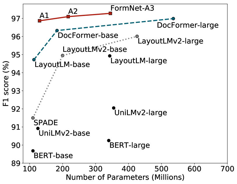
Figure 7: Model Size vs. Entity Extraction F1 Score on CORD benchmark. The proposed FormNets significantly outperform other recent approaches – FormNet-A2 achieves higher F1 score (97.10%) while using a 2.5x smaller model and 7.1x less pre-training data than DocFormer (96.99%; Appalaraju et al., 2021). FormNet-A3 obtains the highest 97.28% F1 score.

4.2 Experimental Setup

Given a document, we first use the BERT-multilingual vocabulary to tokenize the extracted OCR words. Super-tokens are then generated by direct graph embedding on these 2D tokens. Next, we use ETC transformer layers to continue to process the super-tokens based on the serialization provided by the corresponding datasets. Please see Appendix A for implementation details.

We use 12-layer GCN and 12-layer ETC in FormNets and scale up the FormNet family with different numbers of hidden units and attention heads to obtain FormNet-A1 (512 hidden units and 8 attention heads), A2 (768 hidden units and 12 attention heads), and A3 (1024 hidden units and 16 attention heads). Ablations on the FormNets can be found in Figure 7 and 8, and Table 4 in Appendix.

MLM Pre-training.

Following Appalaraju et al. (2021), we collect around 700k unlabeled form documents for unsupervised pre-training. We adopt the Masked Language Model (MLM) objective Taylor (1953); Devlin et al. (2019) to pre-train the networks. This forces the networks to reconstruct randomly masked tokens in a document to learn the underlying semantics of language from the pre-training corpus. We train the models from scratch using Adam optimizer with batch size of 512. The learning rate is set to 0.0002 with a warm-up proportion of 0.01.

Fine-tuning.

We fine-tune all models in the experiments using Adam optimizer with batch size of 8. The learning rate is set to 0.0001 without warm-up. We use cross-entropy loss for the multi-class BIOES tagging tasks. The fine-tuning is conducted on Tesla V100 GPUs for approximately 10 hours on the largest corpus. Note that we only apply the MLM pre-training for the experiments on CORD and FUNSD as in Xu et al. (2020, 2021). For the experiments on Payment, we follow Majumder et al. (2020) to directly train all networks from scratch without pre-training.

4.3 Results

Benchmark Comparison.

Table 1 lists the results that are based on the same evaluation protocal. The proposed FormNet achieves the new best F1 scores on CORD, FUNSD, and Payment benchmarks. Figure 7 shows model size vs. F1 score for all recent approaches. On CORD and FUNSD, FormNet-A2 (Table 4 in Appendix) outperforms the most recent DocFormer Appalaraju et al. (2021) while using a 2.5x smaller model and 7.1x less unlabeled pre-training documents. On the larger CORD, FormNet-A3 continues to improve the performance to the new best 97.28% F1. In addition, we observe no difficulty training the FormNet from scratch on the Payment dataset. These demonstrate the parameter efficiency and the training sample efficiency of the proposed FormNet.

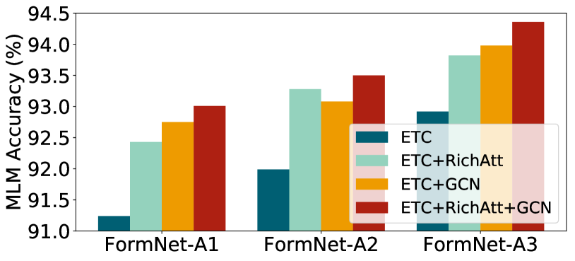
Figure 8: Performance of the MLM pre-training. Both the proposed Rich Attention (RichAtt) and Super-Token by Graph Convolutional Network (GCN) components improve upon ETC Ainslie et al. (2020) baseline by a large margin, showing the effectiveness of their structural encoding capability on large-scale form documents.

	RichAtt	GCN	P	R	F1
CORD			91.40	91.75	91.57
	✓		97.28	95.19	96.03
		✓	96.50	95.13	95.81
	✓	✓	97.50	96.25	96.87
FUNSD			69.24	62.86	65.90
	✓		82.16	82.28	82.22
		✓	78.83	79.93	79.37
	✓	✓	84.17	84.88	84.53

Table 2: Ablation of the proposed Rich Attention (RichAtt) and Super-Token by Graph Convolutional Network (GCN) in entity-level precision, recall, and F1 score on CORD and FUNSD benchmarks using FormNet-A1. Both RichAtt and GCN significantly improve upon ETC Ainslie et al. (2020) baseline by a large margin.

Effect of Structural Encoding in Pre-training.

We study the importance of the proposed Rich Attention and Super-Token by GCN on the large-scale MLM pre-training task across three FormNets as summarized in Figure 8. Both Rich Attention and GCN components improve upon the ETC Ainslie et al. (2020) baseline on reconstructing the masked tokens by a large margin, showing the effectiveness of their structural encoding capability on form documents. The best performance is obtained by incorporating both.

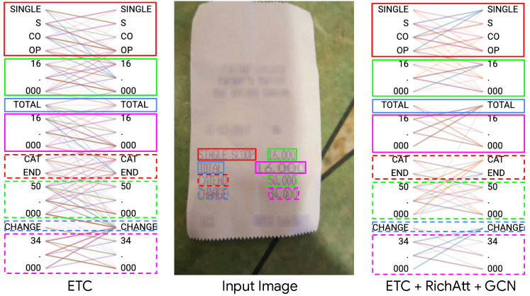
Figure 9: The attention scores for ETC and ETC+RichAtt+GCN models. Unlike the ETC model, the ETC+RichAtt+GCN model makes tokens attend to other tokens within the same visual blocks, along with tokens aligned horizontally, thus strongly leveraging structural cues.

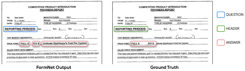
Figure 10: The ambiguous cases where the FormNet predictions do not match the human-annotated ground truth. In this visualization we only showcase mismatched entities.

Effect of Structural Encoding in Fine-tuning.

We ablate the effect of the proposed Rich Attention and Super-Tokens by GCN on the fine-tuning tasks and measure their entity-level precision, recall, and F1 scores. In Table 2, we see that both Rich Attention and GCN improve upon the ETC Ainslie et al. (2020) baseline on all benchmarks. In particular, Rich Attention brings 4.46 points and GCN brings 4.24 points F1 score improvement over the ETC baseline on CORD. We also see a total of 5.3 points increase over the baseline when using both components, showing their orthogonal effectiveness of encoding structural patterns. More ablation can be found in Section B and Table 5 in Appendix.

4.4 Visualization

Using BertViz (Vig, 2019), we visualize the local-to-local attention scores for specific examples of the CORD dataset for the ETC baseline and the ETC+RichAtt+GCN (FormNet) models. Qualitatively in Figure 9, we notice that the tokens attend primarily to other tokens within the same visual block for ETC+RichAtt+GCN. Moreover for that model, specific attention heads are attending to tokens aligned horizontally, which is a strong signal of meaning for form documents. No clear attention pattern emerges for the ETC model, suggesting the Rich Attention and Super-Token by GCN enable the model to learn the structural cues and leverage layout information effectively. More visualization examples are given in the Appendix E. We also show sample model outputs in Figure 10.

5 Conclusion

We present a novel model architecture for key entity extraction for forms, FormNet. We show that the proposed Rich Attention and Super-Token components help the ETC transformer to excel at form understanding in spite of noisy serialization, as evidenced quantitatively by its state-of-the-art performance on three benchmarks and qualitatively by its more sensible attention patterns. In the future, we would like to explore multi-modality input such as images.

Appendix A Implementation Details

The proposed FormNet consists of a GCN encoder to generate structure-aware super-tokens followed by a ETC transformer decoder equipped with Rich Attention for key information extraction. Each GCN layer is a 2-layer multi-layer Perceptron (MLP) with the same number of hidden units as the ETC transformer. The maximum number of neighbors is set to 8 so the graph convolution computation grows linearly w.r.t. the number of vertices. An 1-head attention aggregation function is used after each message passing. We also adopt skip-connection and layer-normalization after each GCN calculation. The ETC transformer takes super-tokens as input. The maximum sequence length is set to 1024. We follow Ainslie et al. (2020) for other hyper-parameter settings.

Appendix B Impact of Super-Tokens by Graph Convolutional Networks

In this experiment, we investigate whether simply increasing the network capacity of the ETC transformer with Rich Attention (RichAtt) can surpass the performance of the FormNet (ETC+RichAtt+GCN). Here ETC-heavy uses 768 hidden units instead of 512 in ETC-standard for both local and global tokens.

Table 3 shows that this is not the case. Simply increasing the network capacity of the ETC transformer from 104M parameters to 187M parameters only improves the performance by 0.7% on FUNSD. On the contrary, the proposed Super-Tokens by GCN continues to improve the standard ETC + RichAtt and outperforms ETC-heavy + RichAtt by a large margin. This evidence suggests that GCN captures the structural information from form documents effectively, which is challenging for ETC due to the limited local radius and multiple text segment issue from imperfect text serialization. These encourage the design of FormNet to balance between efficiency of modeling long documents (ETC) and effectiveness of modeling structural information (GCN).

Model	F1	#Params
ETC-standard + RichAtt	82.22	104M
ETC-heavy + RichAtt	82.92	187M
ETC-standard + RichAtt + GCN	84.53	131M

Table 3: The impact of Super-Tokens by Graph Convolutional Networks (GCNs) compared to heavier ETC transformers. The proposed FormNet (ETC-standard + RichAtt + GCN) significantly outperforms the ETC-heavy + RichAtt counterparts while using much less number of parameters, showing the effectiveness of the structural modeling capability of GCN.

Appendix C Rich Attention Derivations

Here we lay out more explicitly the assumptions and steps needed to derive Rich Attention. First, we assume that there is a latent categorical attention feature $a_{ij}\in\{0,1\}$ that indicates the presence or absence of some unique relevant relationship between tokens $i$ and $j$. In the context of transformers, when $a_{ij}=1$ (abbreviated simply $a_{ij}$), the “value” hidden state $\mathbf{v}_{j}$ gets combined with token $i$’s context representation and propagated up the network.

$$\mathbf{c}_{i} =\sum\limits_{j}\left[a_{ij}\mathbf{v}_{j}\right]$$

However, since categorical variables are discrete (therefore undifferentiable), we use the (differentiable) probability of $a_{ij}$ to compute the expected value state instead.

$$E[\mathbf{c}_{i}] =\sum\limits_{j}\left[P(a_{ij}\mid\mathbf{h}_{i},\mathbf{h}_{j},\ldots)\mathbf{v}_{j}\right]$$

The expressions for $P(a_{ij}\mid\mathbf{h}_{i},\mathbf{h}_{j})$ and $P(a_{ij}\mid f_{ij},\mathbf{h}_{i},\mathbf{h}_{j})$ derived in Section 3.2 are repeated below, again letting $L(X)=\ln(P(X))$ for readability.

$$P(a_{ij}\mid\mathbf{h}_{i},\mathbf{h}_{j})=\text{soft}\max_{j}($$

$$\qquad L(\mathbf{h}_{i},\mathbf{h}_{j}\mid a_{ij})+L(a_{ij}))_{i}$$

$$P(a_{ij}\mid f_{ij},\mathbf{h}_{i},\mathbf{h}_{j})=\text{soft}\max_{j}($$

$$\qquad L(f_{ij}\mid\mathbf{h}_{i},\mathbf{h}_{j},a_{ij})+L(\mathbf{h}_{i},\mathbf{h}_{j}\mid a_{ij})+L(a_{ij}))$$

Note that here and in future derivations, we only care about the case when $a_{ij}=1$, meaning the value of $a_{ij}$ is constant and can be effectively ignored. Theorem 1 shows how to derive dot-product attention, Theorem 2 solves for a binary-valued feature, and Theorem 3 solves for a real-valued feature on an exponential scale; we leave the derivation for other feature types and probability distributions as a fun exercise for the reader.

Appendix D Examples of $\beta$-skeleton Graphs

Figure 11 shows a constructed $\beta$-skeleton graph on the public FUNSD dataset. By using the “ball-of-sight” strategy, $\beta$-skeleton graph offers high connectivity between word vertices for necessary message passing while being much sparser than fully-connected graphs for efficient forward and backward computations.

Appendix E Additional Attention Visualization

Figure 12 shows additional attention visualization. The ETC+RichAtt+GCN model has very interpretable attention scores due to its ability to leverage spatial cues. As a result, the model strongly attends to tokens in the same visual blocks, or that have horizontal alignment. Specific heads also have specific roles: the pink head attends to the token on the right (reading order) within a block and captures intra-block semantics. The blue head attends to the previous horizontally-aligned block (in Figure 12, the tokens "To", "fal", "1560" and "00" all attend to the token "Sub") and captures inter-block semantics.

Dataset	#Samples	FormNet	P	R	F1
FUNSD	199	A1	84.17	84.88	84.53
		A2	85.21	84.18	84.69
CORD	1,000	A1	97.50	96.25	96.87
		A2	97.51	96.70	97.10
		A3	98.02	96.55	97.28

Table 4: Scaling the FormNet family on CORD and FUNSD benchmarks. FormNet-A2 outperforms the most recent DocFormer Appalaraju et al. (2021) on both datasets while being a 2.5x smaller model. On the larger CORD dataset, FormNet-A3 continues to boost the performance to the new best 97.28% F1.

	RichAtt	GCN	P	R	F1
Payment			83.91	83.27	83.58
	✓		92.10	91.48	91.79
		✓	87.79	84.47	86.10
	✓	✓	92.70	91.69	92.19

Table 5: Ablation of the proposed Rich Attention (RichAtt) and Super-Token by Graph Convolutional Network (GCN) in entity-level precision, recall, and F1 score on the Payment benchmark using FormNet-A2. Both RichAtt and GCN significantly improve upon ETC Ainslie et al. (2020) baseline by a large margin.

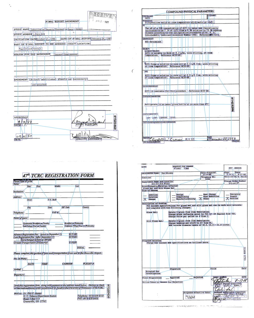
Figure 11: Illustrations of word-level $\beta$-skeleton graph of FUNSD documents. $\beta$-skeleton graphs provide structurally meaningful connectivity between vertices for effective message passing during representation learning and inference.

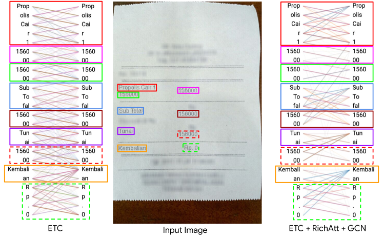
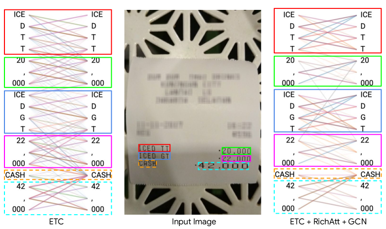
Figure 12: Examples of attention scores on CORD documents for ETC and ETC+RichAtt+GCN models. Unlike the ETC model, the ETC+RichAtt+GCN model makes tokens attend to other tokens within the same visual blocks, along with tokens aligned horizontally, thus strongly leveraging structural cues.

Theorem 1.

If $\mathbf{h}_{i},\mathbf{h}_{j}\mid a_{ij}$ are normally distributed, then $L(\mathbf{h}_{i},\mathbf{h}_{j}\mid a_{ij};\mu,\Sigma)\approx\mathbf{q}_{i}^{\top}\mathbf{k}_{j}+c_{i}$, where $\mathbf{q}_{i}=\text{affine}^{(q)}(\mathbf{h}_{i})$ and $\mathbf{k}_{j}=\text{affine}^{(k)}(\mathbf{h}_{j})$.

Proof.

We partition the parameters of the normal distribution into blocks. Because the covariance matrix is positive definite, the “key-key” block must be positive definite as well, meaning it can be decomposed into a single matrix multiplied times its transpose. We expand the probability into the Gaussian probability density function and apply the natural logarithm – canceling out the $\exp$ function – and put the normalization constant in a separate $c$ term.

$$\mu =\left[\begin{matrix}\mathbf{b}^{(q)}\\ \mathbf{b}^{(k)}\end{matrix}\right]$$

$$\Sigma^{-1} =\left[\begin{matrix}V&W^{\top(q)}W^{(k)}\\ W^{\top(k)}W^{(q)}&W^{\top(k)}W^{(k)}\end{matrix}\right]$$

$$P(\mathbf{h}_{i},\mathbf{h}_{j}\mid a_{ij};\mu,\Sigma) =\frac{1}{\sqrt{\tau^{2d}|\Sigma|}}\exp\left(-\frac{1}{2}([\mathbf{h}_{i};\mathbf{h}_{j}]-\mu)^{\top}\Sigma^{-1}([\mathbf{h}_{i};\mathbf{h}_{j}]-\mu)\right)$$

$$L(\mathbf{h}_{i},\mathbf{h}_{j}\mid a_{ij};\mu,\Sigma) =c-\frac{1}{2}([\mathbf{h}_{i};\mathbf{h}_{j}]-\mu)^{\top}\Sigma^{-1}([\mathbf{h}_{i};\mathbf{h}_{j}]-\mu)$$

From here, we distribute the bilinear transformation and simplify. The result is dot product attention with an ignoreable constant $c_{i}$ (because it later divides out of the softmax function) and an extra bias term composed from the “key” representation alone. We do not explore the effect of this newly-derived bias term in this work.

$$L(\mathbf{h}_{i},\mathbf{h}_{j}\mid a_{ij}) =c-\frac{1}{2}\left(\mathbf{h}_{i}-\mathbf{b}^{(q)}\right)^{\top}V\left(\mathbf{h}_{i}-\mathbf{b}^{(q)}\right)$$

$$\qquad+\left(\mathbf{h}_{i}-\mathbf{b}^{(q)}\right)^{\top}W^{\top(q)}W^{(k)}\left(\mathbf{h}_{j}-\mathbf{b}^{(k)}\right)$$

$$\qquad-\frac{1}{2}\left(\mathbf{h}_{j}-\mathbf{b}^{(k)}\right)^{\top}W^{\top(k)}W^{(k)}\left(\mathbf{h}_{j}-\mathbf{b}^{(k)}\right)$$

$$=c_{i}+\left(\mathbf{h}_{i}-\mathbf{b}^{(q)}\right)^{\top}W^{\top(q)}W^{(k)}\left(\mathbf{h}_{j}-\mathbf{b}^{(k)}\right)$$

$$\qquad-\frac{1}{2}\left(\mathbf{h}_{j}-\mathbf{b}^{(k)}\right)^{\top}W^{\top(k)}W^{(k)}\left(\mathbf{h}_{j}-\mathbf{b}^{(k)}\right)$$

$$=c_{i}+\left(W^{(q)}\mathbf{h}_{i}+W^{(q)}\mathbf{b}^{(q)}\right)^{\top}\left(W^{(k)}\mathbf{h}_{j}+W^{(k)}\mathbf{b}^{(k)}\right)$$

$$\qquad-\frac{1}{2}\left(W^{(k)}\mathbf{h}_{j}+W^{(k)}\mathbf{b}^{(k)}\right)^{\top}\left(W^{(k)}\mathbf{h}_{j}+W^{(k)}\mathbf{b}^{(k)}\right)$$

$$\mathbf{q}_{i} =\text{affine}^{(q)}(\mathbf{h}_{i})$$

$$\mathbf{k}_{j} =\text{affine}^{(k)}(\mathbf{h}_{j})$$

$$L(\mathbf{h}_{i},\mathbf{h}_{j}\mid a_{ij}) =c_{i}+\mathbf{q}_{i}^{\top}\mathbf{k}_{j}-\frac{1}{2}\mathbf{k}_{j}^{\top}\mathbf{k}_{j}$$

$$\approx c_{i}+\mathbf{q}_{i}^{\top}\mathbf{k}_{j}$$

∎

Lemma 1.

If $\mathbf{x}\mid f$ is normally distributed, and $f$ is categorical, then $L(\mathbf{x}\mid f=y;\mu_{y},\Sigma_{y})=\text{biaffine}_{y}(\mathbf{x})$.

Proof.

This can be shown by simply expanding out the probability density function for the normal distribution – with parameters specific to the value $f$ takes – and simplifying. The matrix $V_{y}$ in the result must be negative definite, but this is of little consequence for what follows.

$$P(\mathbf{x}\mid f=y;\mu_{y},\Sigma_{y}) =\frac{1}{\sqrt{\tau^{d}|\Sigma_{y}|}}\exp\left(-\frac{1}{2}(\mathbf{x}-\mu_{y})^{\top}\Sigma_{y}^{-1}(\mathbf{x}-\mu_{y})\right)$$

$$L(\mathbf{x}\mid f) =\mathbf{x}^{\top}\left(-\frac{1}{2}\Sigma_{y}^{-1}\right)\mathbf{x}+\left(\mu_{y}^{\top}\Sigma_{y}^{-1}\right)\mathbf{x}+\left(-\frac{1}{2}\mu_{y}^{\top}\Sigma_{y}^{-1}\mu_{y}-\frac{1}{2}\ln\big{(}\tau^{d}|\Sigma_{y}|\big{)}\right)$$

$$=\mathbf{x}^{\top}V_{y}\mathbf{x}+\mathbf{w}_{y}^{\top}\mathbf{x}+b_{y}$$

$$=\text{biaffine}_{y}(\mathbf{x})$$

∎

Lemma 2.

If $f\mid\mathbf{x}$ is Bernoulli-distributed and $\mathbf{x}\mid f$ is normally distributed, then $P(f\mid\mathbf{x};p,\mu_{0},\mu_{1},\Sigma_{0},\Sigma_{1})=\text{sigmoid}(\text{biaffine}(\mathbf{x}))$, and if $\Sigma_{0}=\Sigma_{1}$, then $=\text{sigmoid}(\text{affine}(\mathbf{x}))$.

Proof.

We begin by applying Bayes’ rule and exponentiating by the log in order to express the probability in terms of the sigmoid function. Then we apply Lemma 1 to expand out the log-likelihood terms, and we use the Bernoulli probability mass function to expand out the log-prior term. This results in the sum of multiple biaffine and constant terms, which is equivalent to a single biaffine function.

$$P(f\mid\mathbf{x};\mu_{0},\mu_{1},\Sigma_{0},\Sigma_{1}) =\frac{P(\mathbf{x}\mid f;\mu_{1},\Sigma_{1})P(f;p)}{P(\mathbf{x}\mid f;\mu_{1},\Sigma_{1})P(f;p)+P(\mathbf{x}\mid\neg f;\mu_{0},\Sigma_{0})P(\neg f;1-p))}$$

$$=\frac{\exp\left(L(\mathbf{x}\mid f)+L(f)\right)}{\exp\left(L(\mathbf{x}\mid f)+L(f)\right)+\exp\left(L(\mathbf{x}\mid\neg f)+L(\neg f)\right)}$$

$$=\text{sigmoid}(L(\mathbf{x}\mid\neg f)+L(\neg f)-(L(\mathbf{x}\mid f)+L(f)))$$

$$=\text{sigmoid}\left(\text{biaffine}_{0}(\mathbf{x})+\ln(1-p)-(\text{biaffine}_{1}+\ln(p))\right)$$

$$=\text{sigmoid}\left(\text{biaffine}(\mathbf{x})\right)$$

Recall from Lemma 1 that the bilinear term $V_{y}$ of the biaffine function is just $-\frac{1}{2}\Sigma_{y}^{-1}$, independent of $\mu_{y}$. Therefore if $\Sigma_{0}=\Sigma_{1}$, then $V_{0}-V_{1}=0$, and the two bilinear terms cancel out when simplifying $\text{biaffine}_{0}-\text{biaffine}_{1}$. Thus in this context, the biaffine function reduces to an affine function.

$$P(f\mid\mathbf{x};p,\mu_{0},\mu_{1},\Sigma_{0},\Sigma_{1}) =\text{sigmoid}\left(\text{affine}(\mathbf{x})\right) \text{ if }\Sigma_{0}=\Sigma_{1}$$

∎

Theorem 2.

If $f_{ij}\mid\mathbf{h}_{i},\mathbf{h}_{j},a_{ij}$ is Bernoulli-distributed, and $\mathbf{h}_{i},\mathbf{h}_{j}\mid f_{ij},a_{ij}$ is normally distributed, and $\Sigma_{0}=\Sigma_{1}$ (as in Lemma 2), then $L(f_{ij}=y\mid\mathbf{h}_{i},\mathbf{h}_{j},a_{ij};\theta)=y\ln(\text{sigmoid}(\text{affine}([\mathbf{h}_{i};\mathbf{h}_{j}])))+(1-y)\ln(1-\text{sigmoid}(\text{affine}([\mathbf{h}_{i};\mathbf{h}_{j}])))$.

Proof.

Because $f_{ij}$ is binary, we begin by expressing the probability mass function in terms of both $f_{ij}$ and $\neg f_{ij}$. Then we apply Theorem 2 to replace the abstract probability term with a fully-specified parametric function. Finally, the natural log can be applied and simplified straightforwardly.

$$P(f_{ij}=y\mid\mathbf{h}_{i},\mathbf{h}_{j},a_{ij};\theta) =P(f_{ij}\mid\mathbf{h}_{i},\mathbf{h}_{j},a_{ij})^{y}(1-P(f_{ij}\mid\mathbf{h}_{i},\mathbf{h}_{j},a_{ij}))^{1-y}$$

$$=\text{sigmoid}(\text{affine}([\mathbf{h}_{i};\mathbf{h}_{j}]))^{y}(1-\text{sigmoid}(\text{affine}([\mathbf{h}_{i};\mathbf{h}_{j}])))^{1-y}$$

$$L(f_{ij}=y\mid\mathbf{h}_{i},\mathbf{h}_{j},a_{ij};\theta) =y\ln(\text{sigmoid}(\text{affine}([\mathbf{h}_{i};\mathbf{h}_{j}])))$$

$$\qquad+(1-y)\ln(1-\text{sigmoid}(\text{affine}([\mathbf{h}_{i};\mathbf{h}_{j}])))$$

∎

Lemma 3.

The log-normal probability density function can be written as $\frac{1}{\sqrt{\tau\sigma^{2}\exp(\sigma^{2})}}\exp\left(-\frac{(\ln(x)-\mu^{\prime})^{2}}{2\sigma^{2}}-\mu^{\prime}\right)$, where $\mu^{\prime}=\mu-\sigma^{2}$.

Proof.

This can be shown through basic algebra.

$$\frac{1}{x\sqrt{\tau\sigma^{2}}}\exp\left(-\frac{(\ln(x)-\mu)^{2}}{2\sigma^{2}}\right) =\frac{1}{\sqrt{\tau\sigma^{2}}}\exp\left(-\frac{(\ln(x)-\mu)^{2}}{2\sigma^{2}}-\ln(x)\right)$$

$$=\frac{1}{\sqrt{\tau\sigma^{2}}}\exp\left(-\frac{(\ln(x)-\mu)^{2}}{2\sigma^{2}}-\frac{2\sigma^{2}\ln(x)}{2\sigma^{2}}\right)$$

$$=\frac{1}{\sqrt{\tau\sigma^{2}}}\exp\left(-\frac{\ln(x)^{2}-2(\mu-\sigma^{2})\ln(x)+\mu^{2}}{2\sigma^{2}}\right)$$

$$=\frac{1}{\sqrt{\tau\sigma^{2}}}\exp\left(-\frac{(\ln(x)-(\mu-\sigma^{2}))^{2}+\sigma^{2}(2\mu-\sigma^{2})}{2\sigma^{2}}\right)$$

$$=\frac{1}{\sqrt{\tau\sigma^{2}}}\exp\left(-\frac{(\ln(x)-(\mu-\sigma^{2}))^{2}}{2\sigma^{2}}-\mu+\frac{\sigma^{2}}{2}\right)$$

$$=\frac{1}{\sqrt{\tau\sigma^{2}}}\exp\left(-\frac{(\ln(x)-\mu^{\prime})^{2}}{2\sigma^{2}}-\mu^{\prime}-\frac{\sigma^{2}}{2}\right)$$

$$=\frac{1}{\sqrt{\tau\sigma^{2}\exp(\sigma^{2})}}\exp\left(-\frac{(\ln(x)-\mu^{\prime})^{2}}{2\sigma^{2}}-\mu^{\prime}\right)$$

∎

Theorem 3.

If $\ln(f_{ij}),\mathbf{h}_{i},\mathbf{h}_{j}\mid a_{ij}$ is normally distributed, then $L(f_{ij}=z\mid\mathbf{h}_{i},\mathbf{h}_{j},a_{ij};\Sigma,\mu)=-\theta^{2}(\ln(z)-\text{affine}([\mathbf{h}_{i};\mathbf{h}_{j}]))^{2}/2-\text{affine}([\mathbf{h}_{i};\mathbf{h}_{j}])$.

Proof.

For convenience and brevity, we stack $\mathbf{h}_{i},\mathbf{h}_{j}$ into one vector $\mathbf{h}_{ij}$. As usual, we apply the probability density function of the assumed probability distribution. Note that here we begin with the joint normal distribution; this allows us to avoid complexities arising from mixing normally- and lognormally-distributed variables.

$$\mathbf{h}_{ij} =[\mathbf{h}_{i};\mathbf{h}_{j}]$$

$$P(\ln(f_{ij})=z,\mathbf{h}_{ij}\mid a_{ij};\mu,\Sigma) =\frac{1}{\sqrt{\tau^{2d+1}|\Sigma|}}\exp\left(([z;\mathbf{h}_{ij}]-\mu)^{\top}\Sigma^{-1}([z;\mathbf{h}_{ij}]-\mu)\right)$$

Similar to Theorem 1, we partition the parameters of the normal distribution into one section for the log-normal feature $\ln(f)$ and one section for the normal features $\mathbf{h}_{ij}$. Then we apply the definition of a conditional normal distribution as described by Eaton (1983) to get the distribution of the new feature conditioned on $\mathbf{h}_{ij}$.

$$\mu =\left[\begin{matrix}b^{(f)}\\ \mathbf{b}^{(h)}\end{matrix}\right]$$

$$\Sigma =\left[\begin{matrix}w^{(ff)}&\mathbf{w}^{\top(hf)}\\ \mathbf{w}^{(hf)}&W^{(hh)}\end{matrix}\right]$$

$$\mu^{\prime} =b^{(f)}+\mathbf{w}^{\top(hf)}W^{-1(hh)}(\mathbf{h}_{ij}-\mathbf{b}^{(h)})$$

$$\sigma^{2\prime} =w^{(ff)}-\mathbf{w}^{\top(hf)}W^{-1(hh)}\mathbf{w}^{(hf)}$$

$$P(\ln(f_{ij})=z\mid\mathbf{h}_{ij},a_{ij};\mu^{\prime},\sigma^{2\prime}) =\frac{1}{\sqrt{\tau\sigma^{2\prime}}}\exp\left(-\frac{(z-\mu^{\prime})^{2}}{2\sigma^{2\prime}}\right)$$

We convert the normal distribution over $\ln(f_{ij})$ into a log-normal distribution over $f_{ij}$ in the convenient form derived in Lemma 3, and simplify its log-probability. Noting that $\mu^{\prime\prime}$ is ultimately an affine function of $\mathbf{h}_{ij}$, whereas $\sigma^{2\prime}$ is composed exclusively from free parameters, we replace the former with an affine function and the latter with a constant $1/\theta^{2}$ (for better numerical stability under gradient-based optimization).

$$P(f_{ij}=z\mid\mathbf{h}_{ij},a_{ij};\mu^{\prime\prime},\sigma^{2\prime}) =\frac{1}{\sqrt{\tau\sigma^{2\prime}\exp(\sigma^{2\prime})}}\exp\left(-\frac{(\ln(z)-\mu^{\prime\prime})^{2}}{2\sigma^{2\prime}}-\mu^{\prime\prime}\right)$$

$$L(f_{ij}=z\mid\mathbf{h}_{ij},a_{ij};\mu^{\prime\prime},\sigma^{2\prime}) =c-\frac{(\ln(z)-\mu^{\prime\prime})^{2}}{2\sigma^{2\prime}}-\mu^{\prime\prime}$$

$$=c-\frac{\theta^{2}(\ln(z)-\text{affine}(\mathbf{h}_{ij}))^{2}}{2}-\text{affine}(\mathbf{h}_{ij})$$

Note that when implementing attention in a neural network, the second instance of the affine term can be absorbed into the affine components of dot-product attention and ignored. ∎

References

- Aggarwal et al. (2020) Milan Aggarwal, Hiresh Gupta, Mausoom Sarkar, and Balaji Krishnamurthy. 2020. Form2seq: A framework for higher-order form structure extraction. In EMNLP.
- Ainslie et al. (2020) Joshua Ainslie, Santiago Ontañón, Chris Alberti, Vaclav Cvicek, Zachary Fisher, Philip Pham, Anirudh Ravula, Sumit Sanghai, Qifan Wang, and Li Yang. 2020. Etc: Encoding long and structured data in transformers. In EMNLP.
- Antonacopoulos et al. (2009) Apostolos Antonacopoulos, David Bridson, Christos Papadopoulos, and Stefan Pletschacher. 2009. A realistic dataset for performance evaluation of document layout analysis. In ICDAR.
- Appalaraju et al. (2021) Srikar Appalaraju, Bhavan Jasani, Bhargava Urala Kota, Yusheng Xie, and R Manmatha. 2021. Docformer: End-to-end transformer for document understanding. In ICCV.
- Bao et al. (2020) Hangbo Bao, Li Dong, Furu Wei, Wenhui Wang, Nan Yang, Xiaodong Liu, Yu Wang, Jianfeng Gao, Songhao Piao, Ming Zhou, et al. 2020. Unilmv2: Pseudo-masked language models for unified language model pre-training. In ICML.
- Chiticariu et al. (2013) Laura Chiticariu, Yunyao Li, and Frederick Reiss. 2013. Rule-based information extraction is dead! long live rule-based information extraction systems! In EMNLP.
- Davis et al. (2019) Brian Davis, Bryan Morse, Scott Cohen, Brian Price, and Chris Tensmeyer. 2019. Deep visual template-free form parsing. In ICDAR.
- Denk and Reisswig (2019) Timo I Denk and Christian Reisswig. 2019. Bertgrid: Contextualized embedding for 2d document representation and understanding. arXiv preprint arXiv:1909.04948.
- Devlin et al. (2019) Jacob Devlin, Ming-Wei Chang, Kenton Lee, and Kristina Toutanova. 2019. BERT: Pre-training of deep bidirectional transformers for language understanding. In NAACL-HLT.
- Dozat (2019) Timothy Dozat. 2019. Arc-factored Biaffine Dependency Parsing. Stanford University.
- Eaton (1983) Morris L Eaton. 1983. Multivariate statistics: a vector space approach. John Wiley & Sons, Inc., 605 Third Ave., New York, NY 10158, USA.
- Garncarek et al. (2020) Łukasz Garncarek, Rafał Powalski, Tomasz Stanisławek, Bartosz Topolski, Piotr Halama, Michał Turski, and Filip Graliński. 2020. Lambert: Layout-aware (language) modeling for information extraction. arXiv preprint arXiv:2002.08087.
- Gilmer et al. (2017) Justin Gilmer, Samuel S Schoenholz, Patrick F Riley, Oriol Vinyals, and George E Dahl. 2017. Neural message passing for quantum chemistry. In ICML.
- Graliński et al. (2020) Filip Graliński, Tomasz Stanisławek, Anna Wróblewska, Dawid Lipiński, Agnieszka Kaliska, Paulina Rosalska, Bartosz Topolski, and Przemysław Biecek. 2020. Kleister: A novel task for information extraction involving long documents with complex layout. arXiv preprint arXiv:2003.02356.
- Ha et al. (1995) Jaekyu Ha, Robert M Haralick, and Ihsin T Phillips. 1995. Recursive xy cut using bounding boxes of connected components. In ICDAR.
- Hirano et al. (2007) Takashi Hirano, Yuichi Okano, Yasuhiro Okada, and Fumio Yoda. 2007. Text and layout information extraction from document files of various formats based on the analysis of page description language. In ICDAR.
- Huang et al. (2019) Zheng Huang, Kai Chen, Jianhua He, Xiang Bai, Dimosthenis Karatzas, Shijian Lu, and CV Jawahar. 2019. Icdar2019 competition on scanned receipt ocr and information extraction. In ICDAR.
- Hwang et al. (2019) Wonseok Hwang, Seonghyeon Kim, Minjoon Seo, Jinyeong Yim, Seunghyun Park, Sungrae Park, Junyeop Lee, Bado Lee, and Hwalsuk Lee. 2019. Post-ocr parsing: building simple and robust parser via bio tagging. In Workshop on Document Intelligence at NeurIPS 2019.
- Hwang et al. (2021) Wonseok Hwang, Jinyeong Yim, Seunghyun Park, Sohee Yang, and Minjoon Seo. 2021. Spatial dependency parsing for semi-structured document information extraction. In ACL-IJCNLP (Findings).
- Jaume et al. (2019) Guillaume Jaume, Hazim Kemal Ekenel, and Jean-Philippe Thiran. 2019. Funsd: A dataset for form understanding in noisy scanned documents. In ICDAR-OST.
- Katti et al. (2018) Anoop Raveendra Katti, Christian Reisswig, Cordula Guder, Sebastian Brarda, Steffen Bickel, Johannes Höhne, and Jean Baptiste Faddoul. 2018. Chargrid: Towards understanding 2d documents. In EMNLP.
- Kirkpatrick and Radke (1985) David G Kirkpatrick and John D Radke. 1985. A framework for computational morphology. In Machine Intelligence and Pattern Recognition. Elsevier.
- Lebourgeois et al. (1992) Frank Lebourgeois, Zbigniew Bublinski, and Hubert Emptoz. 1992. A fast and efficient method for extracting text paragraphs and graphics from unconstrained documents. In ICPR.
- Lee et al. (2021) Chen-Yu Lee, Chun-Liang Li, Chu Wang, Renshen Wang, Yasuhisa Fujii, Siyang Qin, Ashok Popat, and Tomas Pfister. 2021. Rope: Reading order equivariant positional encoding for graph-based document information extraction. In ACL-IJCNLP.
- Liu et al. (2019a) Xiaojing Liu, Feiyu Gao, Qiong Zhang, and Huasha Zhao. 2019a. Graph convolution for multimodal information extraction from visually rich documents. In NAACL-HLT.
- Liu et al. (2019b) Yinhan Liu, Myle Ott, Naman Goyal, Jingfei Du, Mandar Joshi, Danqi Chen, Omer Levy, Mike Lewis, Luke Zettlemoyer, and Veselin Stoyanov. 2019b. Roberta: A robustly optimized bert pretraining approach. arXiv preprint arXiv:1907.11692.
- Luong et al. (2012) Minh-Thang Luong, Thuy Dung Nguyen, and Min-Yen Kan. 2012. Logical structure recovery in scholarly articles with rich document features. In Multimedia Storage and Retrieval Innovations for Digital Library Systems. IGI Global.
- Majumder et al. (2020) Bodhisattwa Prasad Majumder, Navneet Potti, Sandeep Tata, James Bradley Wendt, Qi Zhao, and Marc Najork. 2020. Representation learning for information extraction from form-like documents. In ACL.
- Marinai et al. (2005) Simone Marinai, Marco Gori, and Giovanni Soda. 2005. Artificial neural networks for document analysis and recognition. IEEE Transactions on pattern analysis and machine intelligence.
- O’Gorman (1993) Lawrence O’Gorman. 1993. The document spectrum for page layout analysis. IEEE Transactions on pattern analysis and machine intelligence.
- Palm et al. (2017) Rasmus Berg Palm, Ole Winther, and Florian Laws. 2017. Cloudscan-a configuration-free invoice analysis system using recurrent neural networks. In ICDAR.
- Park et al. (2019) Seunghyun Park, Seung Shin, Bado Lee, Junyeop Lee, Jaeheung Surh, Minjoon Seo, and Hwalsuk Lee. 2019. Cord: A consolidated receipt dataset for post-ocr parsing. In Workshop on Document Intelligence at NeurIPS 2019.
- Parmar et al. (2018) Niki Parmar, Ashish Vaswani, Jakob Uszkoreit, Lukasz Kaiser, Noam Shazeer, Alexander Ku, and Dustin Tran. 2018. Image transformer. In ICML.
- Peng et al. (2017) Nanyun Peng, Hoifung Poon, Chris Quirk, Kristina Toutanova, and Wen-tau Yih. 2017. Cross-sentence n-ary relation extraction with graph lstms. Transactions of the Association for Computational Linguistics (TACL).
- Powalski et al. (2021) Rafał Powalski, Łukasz Borchmann, Dawid Jurkiewicz, Tomasz Dwojak, Michał Pietruszka, and Gabriela Pałka. 2021. Going full-tilt boogie on document understanding with text-image-layout transformer. In ICDAR.
- Qian et al. (2019) Yujie Qian, Enrico Santus, Zhijing Jin, Jiang Guo, and Regina Barzilay. 2019. GraphIE: A graph-based framework for information extraction. In NAACL-HLT.
- Raffel et al. (2020) Colin Raffel, Noam Shazeer, Adam Roberts, Katherine Lee, Sharan Narang, Michael Matena, Yanqi Zhou, Wei Li, and Peter J Liu. 2020. Exploring the limits of transfer learning with a unified text-to-text transformer. Journal of Machine Learning Research (JMLR).
- Ratinov and Roth (2009) Lev Ratinov and Dan Roth. 2009. Design challenges and misconceptions in named entity recognition. In Conference on Computational Natural Language Learning (CoNLL).
- Schuster et al. (2013) Daniel Schuster, Klemens Muthmann, Daniel Esser, Alexander Schill, Michael Berger, Christoph Weidling, Kamil Aliyev, and Andreas Hofmeier. 2013. Intellix–end-user trained information extraction for document archiving. In ICDAR.
- Serrano and Smith (2019) Sofia Serrano and Noah A Smith. 2019. Is attention interpretable? arXiv preprint arXiv:1906.03731.
- Shaw et al. (2018) Peter Shaw, Jakob Uszkoreit, and Ashish Vaswani. 2018. Self-attention with relative position representations. In NAACL-HLT.
- Shilman et al. (2005) Michael Shilman, Percy Liang, and Paul Viola. 2005. Learning nongenerative grammatical models for document analysis. In ICCV.
- Simon et al. (1997) Anikó Simon, J-C Pret, and A Peter Johnson. 1997. A fast algorithm for bottom-up document layout analysis. IEEE Transactions on Pattern Analysis and Machine Intelligence.
- Song et al. (2018) Linfeng Song, Yue Zhang, Zhiguo Wang, and Daniel Gildea. 2018. N-ary relation extraction using graph state lstm. arXiv preprint arXiv:1808.09101.
- Soto and Yoo (2019) Carlos Soto and Shinjae Yoo. 2019. Visual detection with context for document layout analysis. In EMNLP-IJCNLP.
- Sutskever et al. (2014) Ilya Sutskever, Oriol Vinyals, and Quoc V Le. 2014. Sequence to sequence learning with neural networks. In NIPS.
- Taylor (1953) Wilson L Taylor. 1953. “cloze procedure”: A new tool for measuring readability. Journalism quarterly.
- Vaswani et al. (2017) Ashish Vaswani, Noam Shazeer, Niki Parmar, Jakob Uszkoreit, Llion Jones, Aidan N Gomez, Ł ukasz Kaiser, and Illia Polosukhin. 2017. Attention is all you need. In NIPS.
- Vig (2019) Jesse Vig. 2019. A multiscale visualization of attention in the transformer model. In ACL: System Demonstrations.
- Wang et al. (2022) Renshen Wang, Yasuhisa Fujii, and Ashok C. Popat. 2022. Post-ocr paragraph recognition by graph convolutional networks. In WACV.
- Wei et al. (2013) Hao Wei, Micheal Baechler, Fouad Slimane, and Rolf Ingold. 2013. Evaluation of svm, mlp and gmm classifiers for layout analysis of historical documents. In ICDAR.
- Xu et al. (2021) Yang Xu, Yiheng Xu, Tengchao Lv, Lei Cui, Furu Wei, Guoxin Wang, Yijuan Lu, Dinei Florencio, Cha Zhang, Wanxiang Che, et al. 2021. Layoutlmv2: Multi-modal pre-training for visually-rich document understanding. In ACL-IJCNLP.
- Xu et al. (2020) Yiheng Xu, Minghao Li, Lei Cui, Shaohan Huang, Furu Wei, and Ming Zhou. 2020. Layoutlm: Pre-training of text and layout for document image understanding. In KDD.
- Yang et al. (2017) Xiao Yang, Ersin Yumer, Paul Asente, Mike Kraley, Daniel Kifer, and C Lee Giles. 2017. Learning to extract semantic structure from documents using multimodal fully convolutional neural networks. In CVPR.
- Yu et al. (2020) Wenwen Yu, Ning Lu, Xianbiao Qi, Ping Gong, and Rong Xiao. 2020. Pick: processing key information extraction from documents using improved graph learning-convolutional networks. In ICPR.
- Zaheer et al. (2020) Manzil Zaheer, Guru Guruganesh, Avinava Dubey, Joshua Ainslie, Chris Alberti, Santiago Ontanon, Philip Pham, Anirudh Ravula, Qifan Wang, Li Yang, et al. 2020. Big bird: Transformers for longer sequences. In NeurIPS.
- Zhang et al. (2019) Kaixuan Zhang, Zejiang Shen, Jie Zhou, and Melissa Dell. 2019. Information extraction from text regions with complex tabular structure. In NeurIPS.
- Zhang et al. (2020) Shi-Xue Zhang, Xiaobin Zhu, Jie-Bo Hou, Chang Liu, Chun Yang, Hongfa Wang, and Xu-Cheng Yin. 2020. Deep relational reasoning graph network for arbitrary shape text detection. In CVPR.
- Zhao et al. (2019) Xiaohui Zhao, Endi Niu, Zhuo Wu, and Xiaoguang Wang. 2019. Cutie: Learning to understand documents with convolutional universal text information extractor. In ICDAR.