Simulated bifurcation assisted by thermal fluctuation

Abstract

Various kinds of Ising machines based on unconventional computing have recently been developed for practically important combinatorial optimization. Among them, the machines implementing a heuristic algorithm called simulated bifurcation have achieved high performance, where Hamiltonian dynamics are simulated by massively parallel processing. To further improve the performance of simulated bifurcation, here we introduce thermal fluctuation to its dynamics relying on the Nosé-Hoover method, which has been used to simulate Hamiltonian dynamics at finite temperatures. We find that a heating process in the Nosé-Hoover method can assist simulated bifurcation to escape from local minima of the Ising problem, and hence lead to improved performance. We thus propose heated simulated bifurcation and demonstrate its performance improvement by numerically solving instances of the Ising problem with up to 2000 spin variables and all-to-all connectivity. Proposed heated simulated bifurcation is expected to be accelerated by parallel processing.

Introduction

Unconventional computing with special-purpose hardware devices for solving combinatorial optimization problems has attracted growing interest due to practical importance. Many combinatorial optimization problems can be mapped onto finding ground states of Ising spin models Barahona1982 ; Lucas2014 , which is referred to as the Ising problem. Special-purpose hardware devices for the Ising problem are called Ising machines. Ising machines utilizing natural phenomena have been developed, such as quantum annealers Kadowaki1998 ; Farhi2000 ; Farhi2001 ; Das2008 ; Albash2018 ; Hauke2020 with superconducting circuits Johnson2011 , coherent Ising machines with pulse lasers Wang2013 ; Marandi2014 ; Inagaki2016 ; Yamamoto2017 ; Honjo2021 , oscillator-based Ising machines Wang2017 ; Wang2019a ; Chou2019 ; Mallick2020 ; Vaidya2022 , and other Ising machines with various systems, such as stochastic nanomagnets Sutton2017 , gain-dissipative systems Kalinin2018 , spatial light modulators Pierangeli2019 , memristor Hopfield neural networks Cai2020 , and spin torque nano-oscillators Houshang2020 ; Albertsson2021 .

Ising machines have also been implemented with special-purpose digital processors Yamaoka2016 ; Tsukamoto2017 ; Aramon2019 ; Okuyama2019 ; Yamamoto2021 ; Patel2020 ; Leleu2021a using simulated annealing (SA) Kirkpatrick1983 and other algorithms. Among such algorithms, simulated bifurcation (SB) is a recently proposed heuristic algorithm Goto2019 . SB originates from numerical simulations of Hamiltonian dynamics with bifurcation that is a classical counterpart of quantum adiabatic bifurcation in nonlinear oscillators Goto2016 ; Goto2019a , which itself has been studied actively Nigg2017 ; Puri2017 ; Zhao2018 ; Goto2018a ; Kewming2020 ; Onodera2020 ; Goto2020b ; Kanao2021 ; Goto2021b . Simulation-based approaches such as SB allow one to deal with dense spin-spin interactions with high precision, which might be challenging for physical implementations. Also, the classical dynamics can be simulated efficiently, unlike quantum dynamics. SB can be accelerated by parallel processing with, e.g., field-programmable gate arrays (FPGAs) Goto2019 ; Tatsumura2019 ; Zou2020 ; Tatsumura2021 , because of its capability of simultaneous updating of variables. Recently proposed variants of SB have achieved faster and more accurate optimization Goto2021 than original SB.

To further improve the performance of SB, here we introduce thermal fluctuation to SB. SA can yield high-accuracy solutions by modeling thermal fluctuation Kirkpatrick1983 , while quantum annealing utilizes quantum fluctuation Kadowaki1998 . These fluctuations can assist escape from local minima of the Ising problem and lead to higher solution accuracy.

Our method is based on the Nosé-Hoover method Nose1984 ; Hoover1985 , which enables simulations of Hamiltonian dynamics at finite temperatures Leimkuhler2004 . Unlike SA, the Nosé-Hoover method does not use random numbers, namely, is deterministic, and thus the simplicity of SB is preserved. We find that a simplified dynamics with only a heating process can improve the performance of SB, where an ancillary dynamical variable in the Nosé-Hoover method is replaced by a constant. We numerically demonstrate this improvement by solving instances of the Ising problem with up to 2000 spin variables and all-to-all connectivity, which corresponds to the Sherrington-Kirkpatrick (SK) model introduced in studies of spin glasses Sherrington1975 ; Parisi1979 ; Parisi1993 . The SK model has been widely used to measure the performance of Ising machines Inagaki2016 ; Aramon2019 ; Honjo2021 ; Goto2019 ; Okuyama2019 ; Goto2021 ; Yamamoto2021 ; Leleu2021a ; Oshiyama2022 . Proposed heated SB is also suitable for massively parallel implementations with, e.g., FPGAs.

Results and discussion

SB with thermal fluctuation. First, we briefly explain the Ising problem and SB. The Ising problem is to find $N$ Ising spins ${s_{i}=\pm 1}$ minimizing a dimensionless Ising energy,

$$E_{\rm Ising} = -\frac{1}{2}\sum^{N}_{i=1}\sum^{N}_{j=1}J_{ij}s_{i}s_{j},$$ (1)

where $J_{ij}$ represents the interactions between $s_{i}$ and $s_{j}$ (${J_{ij}=J_{ji}}$ and ${J_{ii}=0}$). The SB has two latest variants, ballistic SB (bSB) and discrete SB (dSB) Goto2021 . Both bSB and dSB are based on the following Hamiltonian equations of motion,

$$\dot{x}_{i} = a_{0}y_{i},$$ (2)

$$\dot{y}_{i} = -\left[a_{0}-a(t)\right]x_{i}+c_{0}f_{i},$$ (3)

where $x_{i}$ and $y_{i}$ are respectively the positions and momenta corresponding to $s_{i}$, the dots denote time derivatives, $a(t)$ is a control parameter, and $a_{0}$ and $c_{0}$ are constants. The force due to the interactions, $f_{i}$, are given by

$$f_{i} = \sum_{j=1}^{N}J_{ij}x_{j},\hskip 35.00005pt\text{for bSB,}$$ (4)

$$f_{i} = \sum_{j=1}^{N}J_{ij}\mathrm{sgn}\left(x_{j}\right),\hskip 10.00002pt\text{for dSB},$$ (5)

where ${\mathrm{sgn}(x_{j})}$ is the sign of $x_{j}$. Time evolutions of $x_{i}$ are calculated by solving Eqs. (2) and (3) with the symplectic Euler method Leimkuhler2004 , where the positions $x_{i}$ are confined within ${\left|x_{i}\right|\leq 1}$ by perfectly inelastic walls at ${x_{i}=\pm 1}$, that is, if ${\left|x_{i}\right|>1}$ after each time step, $x_{i}$ and $y_{i}$ are set to ${x_{i}=\mathrm{sgn}\left(x_{i}\right)}$ and ${y_{i}=0}$. With increasing $a(t)$ from zero to $a_{0}$, bifurcations to ${x_{i}=\pm 1}$ occur, and the signs ${s_{i}=\mathrm{sgn}\left(x_{i}\right)}$ yield a solution to the Ising problem. A solution at the final time is at least a local minimum of the Ising problem Goto2021 . Ballistic behavior in bSB leads to fast convergence to a local or approximate solution, while the discretized $f_{i}$ in dSB enable higher solution accuracy with a longer time.

Here we apply the Nosé-Hoover method Nose1984 ; Hoover1985 ; Leimkuhler2004 with a finite temperature $T$ to Eqs. (2) and (3), obtaining

$$\dot{x}_{i} = a_{0}y_{i},$$ (6)

$$\dot{y}_{i} = -\left[a_{0}-a(t)\right]x_{i}+c_{0}f_{i}-\xi y_{i},$$ (7)

$$\dot{\xi} = \frac{1}{M}\left(\sum_{i=1}^{N}y_{i}^{2}-NT\right),$$ (8)

where $\xi$ is an ancillary variable playing a role of thermal fluctuation, and $M$ is a parameter (mass). The variable $\xi$ controls an instantaneous temperature defined by

$$T_{\rm inst} = \frac{1}{N}\sum_{i=1}^{N}y_{i}^{2},$$ (9)

to be a given $T$ as follows. When $T_{\rm inst}$ is smaller than $T$, $\dot{\xi}$ is negative according to Eq. (8), which makes $\xi$ negative. Then ${|y_{i}|}$ increase owing to the last term in Eq. (7), and thus $T_{\rm inst}$ increases and approaches $T$, which can be regarded as heating. To the contrary, when ${T_{\rm inst}>T}$, cooling occurs.

We found that SB gives better solutions when $\xi$ is kept negative by negative initial $\xi$ and large $M$ (leading to ${\dot{\xi}\simeq 0}$). This observation suggests that the heating can improve SB but the cooling is unnecessary. This may be because increased ${\left|y_{i}\right|}$ by the heating can lead to escape from local minima of the Ising problem. Furthermore, small ${|\dot{\xi}|}$ due to large $M$ above implies that constant $\xi$ can play a similar role, and then we found that $\xi$ replaced by a negative constant $-\gamma$ ${(\gamma>0)}$ can rather yield higher performance. The constant $\gamma$ is regarded as a rate of the heating.

Thus, in this paper, we propose SB with a heating term, which we call heated bSB (HbSB) and dSB (HdSB), as follows,

$$\dot{x}_{i} = a_{0}y_{i},$$ (10)

$$\dot{y}_{i} = -\left[a_{0}-a(t)\right]x_{i}+c_{0}f_{i}+\gamma y_{i}.$$ (11)

We numerically solve Eqs. (10) and (11) by discretizing the time by ${t_{k+1}=t_{k}+\Delta t}$ with a time interval $\Delta t$, and by calculating $x_{i}\left(t_{k+1}\right)$ and $y_{i}\left(t_{k+1}\right)$ from $x_{i}\left(t_{k}\right)$ and $y_{i}\left(t_{k}\right)$ in each time step. Here note that the symplectic Euler method is not applicable for Eqs. (10) and (11), because these equations are no longer Hamiltonian equations owing to the term $\gamma y_{i}$ Leimkuhler2004 . We empirically found that solution accuracy can be improved by the same update as previous bSB and dSB Goto2021 followed by an update corresponding to the term $\gamma y_{i}$. This ordering results in nonzero momenta by the heating and can prevent from getting stuck at the walls. See Methods for a detailed algorithm.

In the following, we compare heated SB with previous SB by solving instances of the Ising problem with all-to-all connectivity, where $J_{ij}$ are randomly chosen from $\pm 1$ with equal probabilities (corresponding to the SK model). The control parameter $a(t)$ is linearly increased from 0 to $a_{0}$. The constant parameters are set as ${a_{0}=1}$ and

$$c_{0} = \frac{c_{1}}{\sqrt{N}},$$ (12)

where $c_{1}$ is a parameter tuned around 0.5, which is based on random matrix theory Goto2019 ; Goto2021 . $x_{i}$ and $y_{i}$ are initialized by uniform random numbers in the interval ${(-1,1)}$.

Performance for a 2000-spin Ising problem. We first solve a benchmark instance called K₂₀₀₀, which is a 2000-spin instance of the Ising problem with all-to-all connectivity Goto2019 ; Goto2021 ; Inagaki2016 ; Yamamoto2021 . K₂₀₀₀ is often expressed as a MAX-CUT problem. The MAX-CUT problem is given by weights $w_{ij}$ with ${w_{ij}=w_{ji}}$, and the following cut value $C$ is maximized,

$$C = \frac{1}{2}\sum_{i=1}^{N}\sum_{j=1}^{N}w_{ij}\frac{1-s_{i}s_{j}}{2}$$ (13)

$$= -\frac{1}{2}E_{\rm Ising}-\frac{1}{4}\sum_{i=1}^{N}\sum_{j=1}^{N}J_{ij},$$ (14)

where in Eq. (14), $C$ has been related to $E_{\rm Ising}$ [Eq. (1)] by ${w_{ij}=-J_{ij}}$. Thus the MAX-CUT problem can be reduced to the Ising problem.

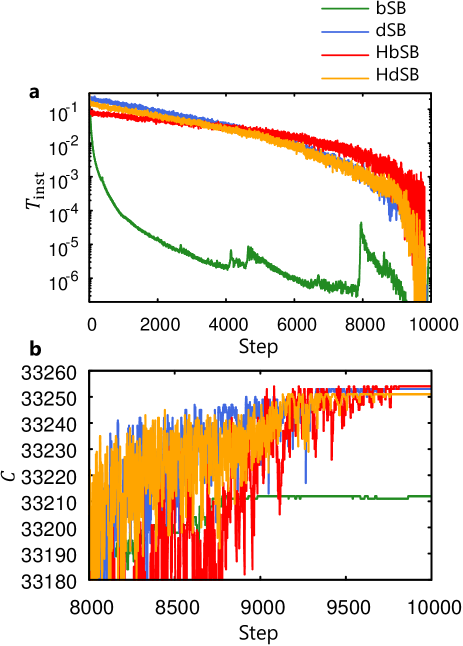
Figure 1: Time evolutions in simulated bifurcation (SB) for a 2000-spin Ising problem (K₂₀₀₀). a Instantaneous temperatures. b Instantaneous cut values. Here, bSB, dSB, HbSB, and HdSB denote ballistic SB, discrete SB, heated bSB, and heated dSB, respectively. Time is represented by time steps. Parameters are ${\Delta t=0.7}$ and ${c_{1}=0.6}$ for bSB, ${\Delta t=1.1}$ and ${c_{1}=0.6}$ for dSB, ${\Delta t=1.1}$, ${c_{1}=0.9}$ and ${\gamma=0.5}$ for HbSB, and ${\Delta t=1.1}$, ${c_{1}=0.7}$ and ${\gamma=0.06}$ for HdSB.

To confirm the effect of the heating, we calculate the instantaneous temperature $T_{\rm inst}$ in Eq. (9) and the cut value $C$ in Eq. (14) at every time step. Figure 1a shows typical examples of time evolutions of $T_{\rm inst}$. Here parameters are the ones optimized in advance, which are explained later. For bSB, $T_{\rm inst}$ rapidly decreases owing to collisions with the perfectly inelastic walls, while $T_{\rm inst}$ for HbSB is kept much higher owing to the heating, as expected. For dSB, $T_{\rm inst}$ is also higher than bSB, because the discretized forces $f_{i}$ in Eq. (5) increase energy, violating conservation of energy Goto2021 . In comparison between HbSB and dSB, $T_{\rm inst}$ for HbSB is higher than dSB around the end of the evolution. HdSB shows similar $T_{\rm inst}$ to dSB, because the optimal rate of the heating $\gamma$ for HdSB is small.

Figure 1b shows last parts of typical time evolutions of $C$. For bSB, $C$ is almost constant for the last 1000 time steps, while $C$ for HbSB continues to fluctuate until nearly the end of the evolution owing to the heating. The fluctuation for HbSB looks similar to the fluctuations for dSB and HdSB.

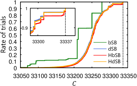
Figure 2: Cumulative distributions of cut values for K₂₀₀₀. The dashed vertical line indicates the best known cut value 33337. Inset shows a magnification around the best known cut value. Here the number of time steps is ${N_{\rm s}=10000}$, and parameters $\Delta t$, $c_{1}$, and $\gamma$ are the same as in Fig. 1. SB means simulated bifurcation, and b, d, and H denote ballistic, discrete, and heated, respectively.

Next, we solve K₂₀₀₀ in 10⁴ trials with random initial $x_{i}$ and $y_{i}$. In one trial, $C$ is evaluated every 100 time steps, and the best value is output. Figure 2 shows examples of cumulative distributions of $C$, where the number of trials giving cut values lower than $C$ are normalized by the total number of trials, 10⁴. For bSB, the majority of trials results in one of a few values of $C$ between 33200 and 33300. On the other hand, dSB, HbSB, and HdSB yield broader distributions, owing to fluctuations (higher instantaneous temperatures) in their dynamics. It is notable that the heating makes the distribution of bSB similar to dSB (and HdSB). Inset in Fig. 2 shows a magnification around the best known cut value, ${C_{\rm best}=33337}$ Goto2021 . The distributions for HbSB and HdSB are shifted to larger $C$ than dSB, indicating improvement by the heating.

We then evaluate average and maximum $C$ in the $10^{4}$ trials and probability $P$ for obtaining $C_{\rm best}$. Here, $P$ is estimated by dividing the number of trials obtaining $C_{\rm best}$ by the total number of trials. Also, using $P$ and the number of time steps, $N_{\rm s}$, we calculate the number of time steps required to find $C_{\rm best}$ with a probability of 99%, which we call step-to-solution $S$, given by

$$S = N_{\rm s}\frac{\log 0.01}{\log(1-P)}.$$ (15)

Step-to-solution is a useful measure of performance of an algorithm Leleu2021a . (Time-to-solution is often used to measure performance of Ising machines Aramon2019 ; Goto2021 ; Leleu2021a ; Patel2020 , but it depends on not only algorithms but also implementations to hardware devices. Time-to-solution equals step-to-solution multiplied by a computation time for one time step.) Here the parameters $\Delta t$, $c_{1}$, and $\gamma$ are set such that $S$ are minimized. For bSB, instead, average $C$ is maximized, because we found $P=0$ for bSB and could not estimate $S$.

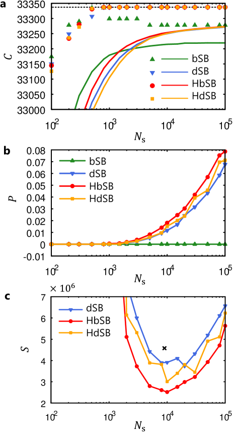
Figure 3: Comparison of performance for K₂₀₀₀. a Average (lines) and maximum (symbols) cut values $C$ as functions of the number of time steps, $N_{\rm s}$. The horizontal dashed line indicates the best known cut value ${C_{\rm best}=33337}$. The maximum $C$ for dSB, HbSB, and HdSB coincide with $C_{\rm best}$ for ${N_{\rm s}\geq 800}$. b Probabilities for obtaining $C_{\rm best}$. c Step-to-solution. The black cross is step-to-solution obtained from previously reported data for dSB Goto2021 . Parameters $\Delta t$, $c_{1}$, and $\gamma$ here are the same as in Fig. 1. SB means simulated bifurcation, and b, d, and H denote ballistic, discrete, and heated, respectively.

Figure 3a shows average and maximum $C$ as functions of $N_{\rm s}$. For large $N_{\rm s}$, average $C$ for dSB, HbSB, and HdSB are larger than that for bSB. $C_{\rm best}$ is reached by three SBs other than bSB. Figure 3b shows that, for large $N_{\rm s}$, $P$ are the highest for HbSB, followed by HdSB, dSB, and bSB in this ordering.

Figure 3c shows $S$ as functions of $N_{\rm s}$. Each SB has a minimum of $S$ at certain $N_{\rm s}$, and in the following we compare $S$ minimized with respect to $N_{\rm s}$. The black cross represents a value obtained from previously reported data for dSB Goto2021 . The present value of $S$ for dSB is smaller than the previous value, because in this study the parameters $\Delta t$ and $c_{1}$ are optimized for K₂₀₀₀ while not in the previous study. In Fig. 3c, at optimal $N_{\rm s}$, $S$ for HbSB is the smallest. Compared with dSB, $S$ are reduced by 32.7% for HbSB and 19.7% for HdSB. These results demonstrate that the heating improves the performance. Although dSB performs better than bSB, bSB is much more improved by the heating than dSB, and resulting HbSB shows higher performance than HdSB.

Performance for 100 instances of a 700-spin Ising problem. Finally we examine the performance for instances other than K₂₀₀₀ by solving 100 instances of the Ising problem with 700 spin variables and all-to-all connectivity Goto2021 ; Leleu2021a . For these instances, reference solutions for estimating step-to-solution were obtained by SA with sufficiently long annealing times and many iterations, which are expected to be close to optimal solutions Goto2021 . Here each instance is solved in $10^{4}$ trials, and $C$ (or $E_{\rm Ising}$) is evaluated at the last time step. We set the parameters to the values optimized in K₂₀₀₀.

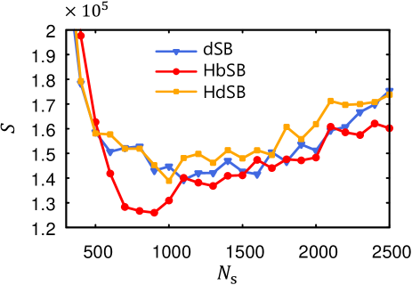
Figure 4: Comparison of performance for 100 instances of a 700-spin Ising problem. The medians of step-to-solution for the 100 instances are shown as functions of the number of time steps, $N_{\rm s}$. Parameters $\Delta t$, $c_{1}$, and $\gamma$ are the same as in Fig. 1. SB means simulated bifurcation, and b, d, and H denote ballistic, discrete, and heated, respectively.

Figure 4 shows the medians of $S$ for the 100 instances Goto2021 ; Leleu2021a as functions of $N_{\rm s}$. HbSB results in the smallest $S$ among four SBs ($S$ by bSB is much larger than those by the others). In comparison with dSB, HbSB reduces $S$ by 9.55%. This result demonstrate that HbSB can improve the performance for not only K₂₀₀₀ but also the other instances.

Conclusion

We have demonstrated that SB can be improved by introducing fluctuation with a heating term, which has been obtained by replacing an ancillary dynamical variable in the Nosé-Hoover method by a constant rate of heating. This heating can be effective for both bSB and dSB, but the improvements are much larger for bSB. We have solved all-to-all connected 2000-spin and 700-spin instances of the Ising problem (the SK model) and have found that HbSB gives better step-to-solution than bSB, dSB, and HdSB. Since proposed heated SB shares the simple dynamics with previous SB, we expect that heated SB will be accelerated by massively parallel processing implemented by, e.g., FPGAs. This study also implies that further improvements of SB will be possible by simple physics-inspired modifications like the heating term introduced here.

METHODS

Heated simulated bifurcation. First, the symplectic Euler method Leimkuhler2004 is formally applied to the terms other than $\gamma y_{i}$ in Eqs. (10) and (11),

$$\tilde{y}_{i} = y_{i}\!\left(t_{k}\right)\!+\!\left\{\!-\!\left[a_{0}\!-\!a\!\left(t_{k}\right)\right]\!x_{i}\!\left(t_{k}\right)\!+\!c_{0}f_{i}\right\}\!\Delta t,$$ (16)

$$\tilde{x}_{i} = x_{i}\!\left(t_{k}\right)\!+\!a_{0}\tilde{y}_{i}\Delta t,$$ (17)

where $f_{i}$ are calculated from ${x_{i}\!\left(t_{k}\right)}$ with Eqs. (4) and (5), and the variables with the tildes denote temporary variables used within a time step. Then, the perfectly inelastic walls work as

$$x_{i}\!\left(t_{k+1}\right) = g\!\left(\tilde{x}_{i}\right),$$ (18)

$$\tilde{\tilde{y}}_{i} = h\!\left(\tilde{x}_{i},\tilde{y}_{i}\right),$$ (19)

where the functions $g(x)$ and $h(x,y)$ are given by

$$g(x) = \left\{\begin{array}[]{cc}x,&|x|\leq 1,\\ 1,&x>1,\\ -1,&x<-1,\end{array}\right.$$ (23)

$$h(x,y) = \left\{\begin{array}[]{cc}y,&|x|\leq 1,\\ 0,&|x|>1.\end{array}\right.$$ (26)

Finally, we include the heating term, referring to the usual Euler method, as

$$y_{i}\!\left(t_{k+1}\right) = \tilde{\tilde{y}}_{i}\!+\!\gamma y_{i}\!\left(t_{k}\right)\!\Delta t.$$ (27)

Equations (16)–(19) and (27) are numerically solved, where the variables are represented as single precision floating-point real numbers.

- (1) Barahona, F. On the computational complexity of Ising spin glass models. J. Phys. A: Math. Gen. 15, 3241–3253 (1982).
- (2) Lucas, A. Ising formulations of many NP problems. Front. Phys. 2, 5 (2014).
- (3) Kadowaki, T. & Nishimori, H. Quantum annealing in the transverse Ising model. Phys. Rev. E 58, 5355–5363 (1998).
- (4) Farhi, E., Goldstone, J., Gutmann, S. & Sipser, M. Quantum computation by adiabatic evolution. Preprint at arXiv:quant-ph/0001106 (2000).
- (5) Farhi, E. et al. A quantum adiabatic evolution algorithm applied to random instances of an NP-complete problem. Science 292, 472–475 (2001).
- (6) Das, A. & Chakrabarti, B. K. Colloquium: Quantum annealing and analog quantum computation. Rev. Mod. Phys. 80, 1061–1081 (2008).
- (7) Albash, T. & Lidar, D. A. Adiabatic quantum computation. Rev. Mod. Phys. 90, 015002 (2018).
- (8) Hauke, P., Katzgraber, H. G., Lechner, W., Nishimori, H. & Oliver, W. D. Perspectives of quantum annealing: methods and implementations. Rep. Prog. Phys. 83, 054401 (2020).
- (9) Johnson, M. W. et al. Quantum annealing with manufactured spins. Nature 473, 194–198 (2011).
- (10) Wang, Z., Marandi, A., Wen, K., Byer, R. L. & Yamamoto, Y. Coherent Ising machine based on degenerate optical parametric oscillators. Phys. Rev. A 88, 063853 (2013).
- (11) Marandi, A., Wang, Z., Takata, K., Byer, R. L. & Yamamoto, Y. Network of time-multiplexed optical parametric oscillators as a coherent Ising machine. Nat. Photonics 8, 937–942 (2014).
- (12) Inagaki, T. et al. A coherent Ising machine for 2000-node optimization problems. Science 354, 603–606 (2016).
- (13) Yamamoto, Y. et al. Coherent Ising machines–optical neural networks operating at the quantum limit. npj Quantum Inf. 3, 49 (2017).
- (14) Honjo, T. et al. 100,000-spin coherent Ising machine. Sci. Adv. 7, eabh0952 (2021).
- (15) Wang, T. & Roychowdhury, J. Oscillator-based Ising machine. Preprint at arXiv:1709.08102 (2017).
- (16) Wang, T. & Roychowdhury, J. in OIM: Oscillator-based Ising machines for solving combinatorial optimisation problems. Unconventional Computation and Natural Computation. UCNC 2019. Lecture Notes in Computer Science, vol 11493, 232–256 (Springer, Cham, 2019).
- (17) Chou, J., Bramhavar, S., Ghosh, S. & Herzog, W. Analog coupled oscillator based weighted Ising machine. Sci. Rep. 9, 14786 (2019).
- (18) Mallick, A. et al. Using synchronized oscillators to compute the maximum independent set. Nat. Commun. 1, 4689 (2020).
- (19) Vaidya, J., Kanthi, R. S. S. & Shukla, N. Creating electronic oscillator-based Ising machines without external injection locking. Sci. Rep. 12, 981 (2022).
- (20) Sutton, B., Camsari, K. Y., Behin-Aein, B. & Datta, S. Intrinsic optimization using stochastic nanomagnets. Sci. Rep. 7, 44370 (2017).
- (21) Kalinin, K. P. & Berloff, N. G. Global optimization of spin Hamiltonians with gain-dissipative systems. Sci. Rep. 8, 17791 (2018).
- (22) Pierangeli, D., Marcucci, G. & Conti, C. Large-scale photonic Ising machine by spatial light modulation. Phys. Rev. Lett. 122, 213902 (2019).
- (23) Cai, F. et al. Power-efficient combinatorial optimization using intrinsic noise in memristor Hopfield neural networks. Nat. Electron. 3, 409–418 (2020).
- (24) Houshang, A. et al. A spin Hall Ising machine. Preprint at arXiv:2006.02236 (2020).
- (25) Albertsson, D. I. et al. Ultrafast Ising machines using spin torque nano-oscillators. Appl. Phys. Lett. 118, 112404 (2021).
- (26) Yamaoka, M. et al. A 20k-spin Ising chip to solve combinatorial optimization problems with CMOS annealing. IEEE J. Solid-State Circuits 51, 303–309 (2016).
- (27) Tsukamoto, S., Takatsu, M., Matsubara, S. & Tamura, H. An accelerator architecture for combinatorial optimization problems. FUJITSU Sci. Tech. J. 53, 8–13 (2017).
- (28) Aramon, M. et al. Physics-inspired optimization for quadratic unconstrained problems using a digital annealer. Front. Phys. 7, 48 (2019).
- (29) Okuyama, T., Sonobe, T., Kawarabayashi, K. & Yamaoka, M. Binary optimization by momentum annealing. Phys. Rev. E 100, 012111 (2019).
- (30) Yamamoto, K. et al. STATICA: A 512-spin 0.25M-weight annealing processor with an all-spin-updates-at-once architecture for combinatorial optimization with complete spin-spin interactions. IEEE J. Solid-State Circuits 56, 165–178 (2021).
- (31) Patel, S., Chen, L., Canoza, P. & Salahuddin, S. Ising model optimization problems on a FPGA accelerated restricted Boltzmann machine. Preprint at arXiv:2008.04436 (2020).
- (32) Leleu, T. et al. Scaling advantage of chaotic amplitude control for high-performance combinatorial optimization. Commun. Phys. 4, 266 (2021).
- (33) Kirkpatrick, S., Gelatt, C. D. & Vecchi, M. P. Optimization by simulated annealing. Science 220, 671–680 (1983).
- (34) Goto, H., Tatsumura, K. & Dixon, A. R. Combinatorial optimization by simulating adiabatic bifurcations in nonlinear Hamiltonian systems. Sci. Adv. 5, eaav2372 (2019).
- (35) Tatsumura, K., Dixon, A. R. & Goto, H. in FPGA-based simulated bifurcation machine. 2019 29th International Conference on Field Programmable Logic and Applications (FPL), 59–66 (IEEE, New York, 2019).
- (36) Zou, Y. & Lin, M. in Massively simulating adiabatic bifurcations with FPGA to solve combinatorial optimization. Proceedings of the 2020 ACM/SIGDA International Symposium on Field-Programmable Gate Arrays (FPGA ’20), 65–75 (ACM, New York, 2020).
- (37) Tatsumura, K., Yamasaki, M. & Goto, H. Scaling out Ising machines using a multi-chip architecture for simulated bifurcation. Nat. Electron. 4, 208–217 (2021).
- (38) Goto, H. et al. High-performance combinatorial optimization based on classical mechanics. Sci. Adv. 7, eabe7953 (2021).
- (39) Goto, H. Bifurcation-based adiabatic quantum computation with a nonlinear oscillator network. Sci. Rep. 6, 21686 (2016).
- (40) Goto, H. Quantum computation based on quantum adiabatic bifurcations of Kerr-nonlinear parametric oscillators. J. Phys. Soc. Jpn. 88, 061015 (2019).
- (41) Nigg, S. E., Lörch, N. & Tiwari, R. P. Robust quantum optimizer with full connectivity. Sci. Adv. 3, e1602273 (2017).
- (42) Puri, S., Andersen, C. K., Grimsmo, A. L. & Blais, A. Quantum annealing with all-to-all connected nonlinear oscillators. Nat. Commun. 8, 15785 (2017).
- (43) Zhao, P. et al. Two-photon driven Kerr resonator for quantum annealing with three-dimensional circuit QED. Phys. Rev. Appl. 10, 024019 (2018).
- (44) Goto, H., Lin, Z. & Nakamura, Y. Boltzmann sampling from the Ising model using quantum heating of coupled nonlinear oscillators. Sci. Rep. 8, 7154 (2018).
- (45) Kewming, M. J., Shrapnel, S. & Milburn, G. J. Quantum correlations in the Kerr Ising model. New J. Phys. 22, 053042 (2020).
- (46) Onodera, T., Ng, E. & McMahon, P. L. A quantum annealer with fully programmable all-to-all coupling via Floquet engineering. npj Quantum Inf. 6, 48 (2020).
- (47) Goto, H. & Kanao, T. Quantum annealing using vacuum states as effective excited states of driven systems. Commun. Phys. 3, 235 (2020).
- (48) Kanao, T. & Goto, H. High-accuracy Ising machine using Kerr-nonlinear parametric oscillators with local four-body interactions. npj Quantum Inf. 7, 18 (2021).
- (49) Goto, H. & Kanao, T. Chaos in coupled Kerr-nonlinear parametric oscillators. Phys. Rev. Research 3, 043196 (2021).
- (50) Nosé, S. A molecular dynamics method for simulations in the canonical ensemble. Molec. Phys. 52, 255–268 (1984).
- (51) Hoover, W. G. Canonical dynamics: Equilibrium phase-space distributions. Phys. Rev. A 31, 1695–1697 (1985).
- (52) Leimkuhler, B. & Reich, S. Simulating Hamiltonian dynamics, (Cambridge University Press, Cambridge, 2004).
- (53) Sherrington, D. & Kirkpatrick, S. Solvable model of a spin-glass. Phys. Rev. Lett. 35, 1792–1796 (1975).
- (54) Parisi, G. Infinite number of order parameters for spin-glasses. Phys. Rev. Lett. 43, 1754–1756 (1979).
- (55) Parisi, G., Ritort, F. & Slanina, F. Critical finite-size corrections for the Sherrington-Kirkpatrick spin glass. J. Phys. A Math. Gen. 26, 247–259 (1993).
- (56) Oshiyama, H. & Ohzeki, M. Benchmark of quantum-inspired heuristic solvers for quadratic unconstrained binary optimization. Sci. Rep. 12, 2146 (2022).