A Squeeze-and-Excitation and Transformer based Cross-task Model for Environmental Sound Recognition

Abstract

Environmental sound recognition (ESR) is an emerging research topic in audio pattern recognition. Many tasks are presented to resort to computational models for ESR in real-life applications. However, current models are usually designed for individual tasks, and are not robust and applicable to other tasks. Cross-task models, which promote unified knowledge modeling across various tasks, have not been thoroughly investigated. In this paper, we propose a cross-task model for three different tasks of ESR: acoustic scene classification, urban sound tagging, and anomalous sound detection. An architecture named SE-Trans is presented that uses attention mechanism-based Squeeze-and-Excitation and Transformer encoder modules to learn channel-wise relationship and temporal dependencies of the acoustic features. FMix is employed as the data augmentation method that improves the performance of ESR. Evaluations for the three tasks are conducted on the recent databases of DCASE challenges. The experimental results show that the proposed cross-task model achieves state-of-the-art performance on all tasks. Further analysis demonstrates that the proposed cross-task model can effectively utilize acoustic knowledge across different ESR tasks.

I Introduction

Humans can automatically recognize sounds, but it is challenging for machines. Audio pattern recognition (APR) is a growing research area where signal processing and machine learning methods are used to understand the surrounding sound. APR is of great importance in automatic speech recognition, automatic music transcription, and environmental sound recognition (ESR). More recently, ESR has attracted much attention due to various applications are emerging in our daily life. For example, heart sound has been used as a biometric to identify a person in a real-time authentication system [1]. In surveillance systems, the detection of gunshots or glass breaking can be used to report danger in time [2]. More meaningful applications are using speech and non-speech audio to detect COVID-19 [3], recognising crying and speech sounds of babies to protect and understand babies [4, 5], and monitoring depression with acoustic and visual features [6].

The Detection and Classification of Acoustic Scenes and Events (DCASE) challenges, which focus on machine listening research for acoustic environments, have dramatically promoted the development of ESR in the past few years [7]. The series of challenges on DCASE have provided a set of tasks, such as acoustic scene classification (ASC) [8], urban sound tagging (UST) [9, 10], and anomalous sound detection (ASD) [11], encouraging the participants to develop strong computational models [12]. The computational models for ESR usually consists of two stages: feature extraction, in which audio is transformed into a feature representation, and sound recognition, in which a mapping between the feature representations and labels of sound classes is learned by a classifier [13]. Log Mel spectrograms, which represent the audio signal using perceptually motivated frequency scales[14], have been the predominant feature representations in this field [15, 16]. Recently, deep learning methods have achieved great success in many pattern recognition fields, including image classification , speech processing, natural language processing (NLP), and ESR [17, 18, 19, 20, 21]. Deep neural networks (DNNs) based classifiers, such as convolutional neural networks (CNNs), convolutional recurrent neural networks (CRNNs), and Transformer, have become dominant approaches in ESR and outperform the conventional machine learning methods [22, 23]. Moreover, data augmentation has been a necessary part of an ESR models to mitigate overfitting during the training stage, and further improves the performance [24].

In DCASE challenges, ESR models are usually developed for concrete and individual tasks, but the unification of the models designed for these tasks has not been adequately studied. Unified models across different domains will facilitate knowledge modeling from these fields, and such unification has been explored in NLP (e.g. Bert [25]), computer vision (CV) (e.g. ViT backbone [26]), and APR (e.g. PANN [27]). Considering the above reason, it is of great importance to explore a generic model that has robust performance and wide applicability for different ESR tasks, where the common acoustic knowledge can be modeled in the model. The models across several tasks in ESR are called cross-task models [28]. They have investigated the performance of CNNs-based models for several tasks of DCASE challenges in 2018 and 2019, and found that a 9-layer CNN with average pooling is a good model for most of the tasks.

Recently, attention mechanism has attracted tremendous interest in numerous pattern recognition fields as a component of DNNs. Implementing attention can get more powerful representations by allowing the networks to dynamically pay attention to the effective information of the signal. For speech emotion recognition, CNN with self-attention mechanism has been used to obtain abundant emotional information on frame-level [29]. In ESR, different attention mechanisms have been applied for environmental sound classification [30], sound event detection[31], and ASC [32]. Yet, to the best of our knowledge, attention mechanism has not been studied or exploited in cross-task models.

In this paper, we propose a cross-task model based on an attention mechanism for modeling on three subtasks of ESR, i.e., ASC, UST, and ASD. First, we propose to use Squeeze-and-Excitation (SE) modules after convolution layers in the main architecture [33]. The model is allowed to learn the importance of channel-wise features, and the acoustic information between channels is effectively enhanced. Next, we adopt the Transformer encoder in our architecture, where the multi-head self-attention (MHSA) mechanism is applied to efficiently model and process the temporal dependencies. In our proposed model, the main architecture is based on SE and Transformer encoder modules, which is called SE-Trans. Besides, we proposed to use FMix as the data augmentation method, which can effectively augment the training data by randomly mixing irregular areas of two samples. The main contributions of this paper can be summarized as follows:

• We propose a cross-task model that can generally model various audio patterns across several tasks of ESR.

• We incorporate two modules with attention mechanisms, i.e., SE and Transformer encoder, into the main architecture to enhance channel-wise acoustic information and catch temporal dependencies.

• We firstly introduce FMix into ESR as the data augmentation method and find FMix can effectively augment the training data and significantly improve the performance of ESR tasks.

• We conduct experiments on the latest dataset of DACSE challenges. And results show that our cross-task model achieves state-of-the-art performance for ASC, UST, and ASD.

The rest of the paper is organized as follows: Section II reviews the related works of this paper. Section III describes the detailed parts of the proposed cross-task model. Section IV presents the experiments, the results and discussions are given in Section V. Finally, we conclude this paper in Section VI.

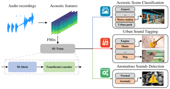
Figure 1: The processing stages of the proposed cross-task model.

II Task description and related works

DCASE challenges have been successfully held seven times since 2013. Several tasks closed to different aspects of real-life applications are brought by the organizers, providing public datasets, metrics, and evaluation frameworks [12]. Among the tasks, ASC, UST, and ASD, which are consecutively organized for at least 2 years, have attracted much interest.

ASC means to identify an acoustic scene among the predefined classes in the environment, using signal processing and machine learning methods. The acoustic scenes are usually recorded in real-life environments such as squares, streets, and restaurants. Many applications can potentially use ASC systems, e.g., wearable devices [34], robotics [35], and smart home devices [36]. Early works primarily focused on using conventional machine learning methods, such as Gaussian mixture models and support vector machines. Gradually, CNNs-based approaches have become the mainstream for designing systems and achieved the top performance in recent years [37, 38].

The goal of UST is to predict whether an urban sound exists in a recording. Various urban sounds occur around us all the time when living in the big cities. Some urban sounds can be harmful if we are exposed to them for a long time, such as traffic noise. Sounds of New York City (SONYC) is a research project investigating data-driven approaches to mitigate urban noise pollution [39]. SONYC has collected over 100 million recordings between 2016 and 2019, and the researchers held the UST tasks in DCASE 2019 and DCASE 2020 to resort to computational methods for automatically monitoring noise pollution. Both of the champions in DCASE 2019 and DCASE 2020 UST tasks used CNNs as the primary architecture of the classifiers [40, 41].

ASD aims to detect anomalous acoustic signals in particular environments. ASD for machine condition monitoring (MCM) is an emerging task to identify whether the sound produced from a target machine is normal or anomalous. Some of the successful methods in ASD can reduce the loss caused by machine damage and speed up the use of essential technologies in industry. In factories, anomalous sounds rarely occur and are often unavailable. The main challenge is to detect unknown anomalous sounds under the condition that only normal sound samples are provided. To address this problem, some researchers organized the tasks named ”unsupervised detection of anomalous sounds for MCM” in DCASE 2020 and DCASE 2021 [42, 11]. In [43], the authors proposed a self-supervised density estimation method using normalizing flows and machine IDs to detect anomalies. A MobileFaceNet was trained in a self-supervised learning manner to detect anomalous sound and achieved great performance in DCASE 2021 [44].

Recently, using deep learning in the above tasks of ESR has become the trend and achieved state-of-the-art performance. Yet, these methods mostly focus on specific tasks, we have observed little relevant literature on studying unification in this field. The study of cross-task tries to find a general model (system) that can perform well for various tasks in ESR, and deep learning based cross-task models have been investigated. Kong et al. proposed DNNs based baseline with the same structure for the DCASE 2016 challenge [45]. The DNNs take Mel-filter bank features as input and outperform the official baselines in many but not all tasks. In DCASE 2018 challenge, they created a cross-task baseline system for all five tasks based on CNNs [46]. CNNs with 4 layers and 8 layers are investigated through performance for various tasks with the same configuration of neural networks. They found that deeper CNN with 8 layers performs better than CNN with 4 layers on almost all tasks. Further, Kong et al. proposed generic cross-task baseline systems, where CNNs with 5, 9, and 13 layers are studied [28]. The results of the CNN models on five tasks of DCASE 2019 showed that the 9-layer CNN with average pooling could achieve good performance in general.

CNNs are designed specifically for images and have become the dominant models in CV [47]. Because of its great ability to extract features from spectrograms, CNNs have also been the most popular architecture in ESR. Most recently, CNNs have incorporated many attention mechanisms, such as SE and self-attention, to focus on key parts, catch long-range dependencies of the input, and reduce computational complexity. The combination of CNNs and attention has outperformed many of the previous methods and become a new research direction. SENet [33] was proposed to explicitly learn the relationships between the channels and pay more attention to the more important feature maps. Implementing SE can effectively improve the performance of classification with little increase of the parameters. In addition, Transformer has extensively achieved state-of-the-art performance in many research domains. The MHSA modules in Transformer can model the input of long sequences and process in parallel. A combination of CNNs and Transformers has been proposed to model both local and global dependencies of an audio sequence for speech recognition [48].

Most state-of-the-art approaches in ESR use data augmentation in the training stage to overcome the overfitting problem caused by the lack of environmental sound. These data augmentation methods can be categorized into two classes, depending on the representation format of sound. In the first class, the methods operate on the sound waveform, including changing the speed, volume, and pitch etc [24]. The drawback of these methods is that they need complex operations and a lot of time to generate enough samples. Another class is usually carried out on the spectrogram without taking too much time to get enough data. These methods are derived from the methods for augmenting images, using two main strategies. One strategy does data augmentation by removing or masking some information on the images or spectrograms (e.g. cutout[49] or SpecAugment [50]). The above strategy is undesirable for some classification tasks because it may lose part of the information during training. Another strategy called mixed sample data augmentation (MSDA) augments the training data by combining samples according to a specific policy, such as mixup[51] and FMix [52]. The MSDA methods can generate more unseen data, force the model to learn more robust features, and finally improve the performance of classification.

III Proposed Method

III-A Model overview

The processing stages of the proposed cross-task model are shown in Fig. 1. First, the model takes audio recordings as input and transforms them into acoustic features. Then, FMix is applied to the acoustic features to generate mixed acoustic features. Next, the SE-Trans, which consists of SE-blocks and a Transformer encoder, is trained to recognize the acoustic features under different situations. For ASC, each audio recording will be recognized as a specific acoustic scene. For UST, each audio recording will be tagged with different urban sound classes. And for ASD, each audio recording will be annotated as normal or anomaly.

III-B SE-block

The first part of the proposed model is SE-blocks. We denote $\mathbf{X}\in\mathbb{R}^{T\times F}$ as an acoustic feature transformed from an audio recording $x$, where $T$ is the number of time frames and $F$ is the number of frequency bins. Then $\mathbf{X}$ is further reshaped into $\mathbf{X}\in\mathbb{R}^{T\times F\times 1}$, which is consecutively processed by convolutional layers (Conv), batch normalization (BN), SE layers, and rectified linear unit (ReLU) for two times in each SE-block.

We assume that the output of BN is $\mathbf{X^{\prime}}=[\mathbf{x^{\prime}}_{1},\mathbf{x^{\prime}}_{2},\cdots,\mathbf{x^{\prime}}_{c}]\in\mathbb{R}^{T^{\prime}\times F^{\prime}\times C}$, where $C$ is the number of channels of the convolutional layer, $T^{\prime}$ is the number of time frames, and $F^{\prime}$ is the number of frequency bins. In an SE layer, $\mathbf{X^{\prime}}$ is first squeezed through time-frequency dimensions $T^{\prime}\times F^{\prime}$ in each channel:

$$z_{c}=f_{sq}\left(\mathbf{x^{\prime}}_{c}\right)=\frac{1}{T^{\prime}\times F^{\prime}}\sum_{i=1}^{T^{\prime}}\sum_{j=1}^{F^{\prime}}\mathbf{x^{\prime}}_{c}(i,j),$$ (1)

where $f_{sq}$ is the global average pooling function, and $z_{c}$ is the channel-wise value of squeezed vector $\mathbf{z}\in\mathbb{R}^{C}$. A channel-wise relationship is then excited from $\mathbf{z}$ by a gating mechanism:

$$\mathbf{w}=f_{ex}(\mathbf{z},\mathbf{W})=\sigma\left(\mathbf{W_{2}}\operatorname{ReLU}\left(\mathbf{W_{1}}\mathbf{z}\right)\right),$$ (2)

where $\mathbf{W_{1}}\in\mathbb{R}^{\frac{C}{r}\times C}$ and $\mathbf{W_{2}}\in\mathbb{R}^{C\times\frac{C}{r}}$ are weights of two fully connected (FC) layers, $r$ is a hyperparameter, $\mathbf{w}$ is the channel-wise weighted vector, $\sigma$ is the sigmoid activation. The channel-wise feature maps of $\mathbf{X^{\prime}}$ are activated by $\mathbf{w}$:

$$\mathbf{x^{\prime\prime}}_{c}=f_{ac}\left(\mathbf{x^{\prime}}_{c},w_{c}\right)=w_{c}\cdot\mathbf{x^{\prime}}_{c},$$ (3)

where $\mathbf{x^{\prime\prime}}_{c}$ and $w_{c}$ are the $c$th channel of $\mathbf{X^{\prime\prime}}\in\mathbb{R}^{T^{\prime}\times F^{\prime}\times C}$ and $\mathbf{w}$, respectively. $f_{ac}$ is a channel-wise multiplication function. Finally, an average pooling layer (Avg Pool) is applied to reduce the size of feature maps. A flowchart of the SE layer is shown in Fig. 2.

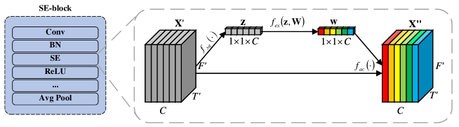
Figure 2: A flowchart of the SE layer in the SE-block. Convolutional layers (Conv), batch normalization (BN), rectified linear units (ReLU), average pooling layer (Avg Pool).

A global average pooling layer is used after the SE-blocks to get a proper input shape of the Transformer encoder. We assumed the input of the Transformer encoder as $\mathbf{O}\in\mathbb{R}^{T^{\prime\prime}\times C}$, where $T^{\prime\prime}$ is the number of time frames.

III-C Transformer encoder

The second part of the SE-Trans is the Transformer encoder. The Transformer is a sequence to sequence model which usually contains an encoder and a decoder. Considering that our proposed cross-task model is used for classification tasks, we only use the encoder.

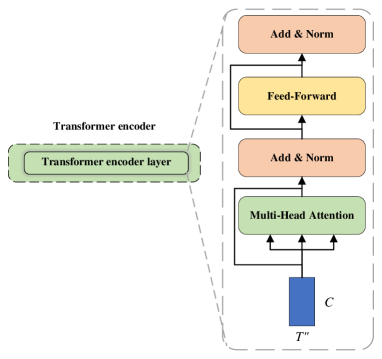
Figure 3: A flowchart of the Transformer encoder layer.

In each encoder, there are several encoder layers. The $T^{\prime\prime}$ and $C$ dimension of $\mathbf{O}$ is the sequence length and feature number of the encoder layer, respectively. Fig. 3 shows a flowchart of the encoder layer in the Transformer encoder. The first part of a Transformer encoder layer is MHSA, which is composed of multiple scaled dot product attention modules. The input is mapped $h$ times with different, learnable linear projections to get parallel queries $\mathbf{Q}_{i}$, keys $\mathbf{K}_{i}$ and values $\mathbf{V}_{i}$ respectively, and this is formulated as:

$$\mathbf{Q}_{i} =\mathbf{O}\mathbf{W}^{Q}_{i}$$ (4)

$$\mathbf{K}_{i} =\mathbf{O}\mathbf{W}^{K}_{i}$$

$$\mathbf{V}_{i} =\mathbf{O}\mathbf{W}^{V}_{i},$$

where $i\in[1,h]$, $\mathbf{W}^{Q}_{i},\mathbf{W}^{K}_{i}\in\mathbb{R}^{C\times d_{k}},\mathbf{W}^{V}_{i}\in\mathbb{R}^{C\times d_{v}}$0

are $i$th linear transformation matrix for mapped queries, keys, and values

$\mathbf{Q}_{i},\mathbf{K}_{i}\in\mathbb{R}^{T^{\prime\prime}\times d_{k}},\mathbf{V}_{i}\in\mathbb{R}^{T^{\prime\prime}\times d_{v}}$.

The dot product of the queries $\mathbf{Q}_{i}$ with all keys $\mathbf{K}_{i}$ is then computed, followed by division of a scaling factor $\sqrt{d_{k}}$. The softmax operation converts the correlation values $\mathbf{V}_{i}$ to probabilities which indicates how much the importance of $\mathbf{V}_{i}$ in a time step should be attended. The output of the scaled dot product attention is computed as a weighted sum of values $\mathbf{V}_{i}$:

$$head_{i}=\operatorname{Attention}\left(\mathbf{Q}_{i},\mathbf{K}_{i},\mathbf{V}_{i}\right)=\operatorname{softmax}\left(\frac{\mathbf{Q}_{i}\mathbf{K}^{\mathrm{T}}_{i}}{\sqrt{d_{k}}}\right)\mathbf{V}_{i}.$$ (5)

The attentions of all heads are concatenated and linearly projected again to obtain the multi-head output:

$$\mathbf{O}_{MH}=\operatorname{Concat}\left(head_{1},\cdots,head_{h}\right)\mathbf{W}^{O},$$ (6)

where $\mathbf{W}^{O}\in\mathbb{R}^{C\times C}$ is a linear transformation matrix. After that, residual connections and layer normalization (LN) [53] are employed:

$$\mathbf{O}_{M}=\operatorname{LN}(\mathbf{O}+\mathbf{O}_{MH}).$$ (7)

The output is fed into the feed-forward network (FFN) followed by a residual connection and LN to get the final output of the Transformer encoder and that is formulated as:

$$\mathbf{O}^{\prime}=\operatorname{LN}\left(\operatorname{FFN}\left(\mathbf{O}_{M}\right)+\mathbf{O}_{M}\right),$$ (8)

where $\mathbf{O}^{\prime}\in\mathbb{R}^{T^{\prime\prime}\times C}$ is the output of the Transformer encoder.

III-D Loss functions

In this section, we describe the loss functions used for ASC, UST, and ASD in the model.

III-D1 Loss of acoustic scene classification

Since the ground truth and prediction of a recording contains only one of the acoustic scene classes, ASC is a multi-class classification task. We denote the output of SE-Trans as $f(\mathbf{X})=[f(\mathbf{X})_{1},\cdots,f(\mathbf{X})_{N}]$, where $N$ is the number of classes. The loss function of ASC is categorical cross-entropy loss, defined as:

$$L_{ASC}(\hat{y},y)=-\sum_{n=1}^{N}y_{n}\log\hat{y}_{n}$$ (9)

where $\hat{y}_{n}=\operatorname{softmax}\left(f(\mathbf{X})_{n}\right)=\frac{e^{f(\mathbf{X})_{n}}}{\sum_{n=1}^{N}e^{f(\mathbf{X})_{n}}}$ is the estimated label and $y_{n}$ is the true label of the $n$th class .

III-D2 Loss of urban sound tagging

While for UST, the ground truth and prediction of a sound recording may contain multiple classes. Therefore, it is a multi-label classification task. The loss function of UST is categorical binary cross-entropy loss, where $f(\mathbf{X})_{n}$ has to pass the $\operatorname{sigmoid}$ activation function to obtain $\hat{y}_{n}$, and the loss is defined as:

$$L_{UST}(\hat{y},y)=-\sum_{n=1}^{N}\left[y_{n}\log\hat{y}_{n}+\left(1-y_{n}\right)\log\left(1-\hat{y}_{n}\right)\right].$$ (10)

III-D3 Loss of anomalous sound detection

For ASD in MCM, we adopt a self-supervised learning strategy to train the model to differentiate different machine IDs of one machine type. Therefore, ASD can be seen as a supervised multi-class classification task. The loss function is categorical cross-entropy loss and the same as defined in Eq. 9, where the $\hat{y}_{n}$ and $y_{n}$ in ASD refer to the estimated and true machine ID, respectively.

III-E Data augmentation

In the proposed cross-task model, we employ FMix as the data augmentation method to improve generalization and prevent overfitting of the neural networks.

We applied FMix to the acoustic features in the training stage, the operations are described as follows. First, we sample a random complex matrix $\mathbf{Z}\in\mathbb{C}^{T\times F}$, having the same size as $\mathbf{X}$, with both the real and imaginary parts of $\mathbf{Z}$ are independent and Gaussian. We then keep the low-frequency components and decay the high-frequency components by applying a low-pass filter on $\mathbf{Z}$. Next, we perform an inverse Fourier transform on the complex tensor $\mathbf{Z}$ and take the real part to obtain a grey-scale image. We assign the top $n$ elements of the grey-scale image a value of 1 and the rest a value of 0, therefore, we can obtain a binary mask by the following method:

$$mask(\lambda,\mathbf{g})[i,j]=\left\{\begin{aligned} 1&,\quad\text{if}\quad\mathbf{g}[i,j]\in\text{top}(\lambda TF,\mathbf{g})\\ 0&,\quad\text{otherwise},\end{aligned}\right.$$ (11)

where $\mathbf{g}$ refers to the grey-scale image, $mask(\lambda,\mathbf{g})$ refers to the binary mask, and $\lambda\in[0,1]$ is a hyperparameter. The $\text{top}(n,x)$ function returns a set containing the top $n$ elements of the input $x$, while $\text{top}(\lambda TF,\mathbf{g})$ means that top $\lambda TF$ elements in $\mathbf{g}$ will be selected. Finally, the mixed feature $\tilde{\mathbf{X}}$ can be obtained from two input features $\mathbf{X}_{i}$ and $\mathbf{X}_{j}$ using the following formulation:

$$\centering\tilde{\mathbf{X}}=mask(\lambda,\mathbf{g})\odot\mathbf{X}_{i}+(1-mask(\lambda,\mathbf{g}))\odot\mathbf{X}_{j},\@add@centering$$ (12)

where $\odot$ denotes the Hadamard product.

IV Experimental procedures

We evaluated the proposed cross-task model for all the tasks on the latest dataset of DCASE challenges.

We first describe details of the cross-task model, and then we introduce the dataset, experimental setups, baseline models, and evaluation metrics for ASC, UST, and ASD in this section.

IV-A Cross-task model

In feature extraction, we used log Mel spectrograms as the common acoustic features. However, we extract the acoustic features with different configurations for individual tasks in order to make a fair comparison. The details of feature extraction are described in the following subsections.

SE-Trans is used as the main architecture, which contains two SE-blocks and one Transformer encoder. Each SE block consists of 2 convolutional layers with the same channels and kernel sizes of $3\times 3$. The number of channels of the first and second SE-block is 64 and 128, respectively. An average pooling layer is applied after each SE-block with kernel sizes of $2\times 2$. Similarly, AdaptiveAvgPool2d layer is applied after that to get a proper input size of $16\ (T^{\prime\prime})\times 128\ (C)$ for the Transformer encoder. We also repeated the experiment with different numbers of heads (4 and 8), layers (1 and 2), and FFN size (16, 32, and 64). Max aggregation function along time frames along with an FC layer are applied to the output of SE-Trans. Adam optimizer with a learning rate of 0.001 is used to optimize the loss function.

Besides FMix, two more data augmentation methods were also analyzed. The first method is SpecAugment, which randomly masks the frequency bins and time frames of the spectrograms. The second method is mixup, whose operations on training samples are expressed as:

$$\centering\tilde{x}=\lambda x_{i}+(1-\lambda)x_{j}\@add@centering$$ (13)

$$\tilde{y}=\lambda y_{i}+(1-\lambda)y_{j},$$ (14)

where $x_{i}$ and $x_{j}$ are the input features, $y_{i}$ and $y_{j}$ are the corresponding target labels, and $\lambda\in[0,1]$ is a random number drawn from the beta distribution.

IV-B Acoustic scene classification

IV-B1 Dataset

The dataset used for ASC is the development set of DCASE 2021 Task1 Subtask A [54]. The organizers used different devices to simultaneously capture audio in 10 acoustic scenes, which are airport, shopping mall, metro station, street pedestrian, public square, street traffic, tram, bus, metro, and park. The development set contains data from 9 devices: A, B, C (3 real devices), and S1-S6 (6 simulated devices). The total number of recordings in the development set is 16,930. The dataset is divided into a training set, which contains 13,962 recordings, and a testing set, which contains 2,968 recordings. Complete details of the development set are shown in Table I.

TABLE I: Statistics of the development set of ASC.

Devices		Development set
Name	Type	Training set	Testing set
A&B&C	real	10,215&749&748	330&329&329
S1-S6	simulated	2,250	1,980
Total		13,962	2,968

IV-B2 Experimental setups

We used log Mel spectrograms as the input features. First, all recordings were resampled to 44,100 Hz. The short-time Fourier transform (STFT) with a Hanning window of 40 ms and a hop size of 20 ms was used to extract the spectrogram. We applied 40 Mel-filter bands on the spectrograms followed by a logarithmic operation to calculate log Mel spectrograms. Each log Mel spectrogram has a shape of $500\times 40$, where 500 is the number of time frames and 40 is the number of frequency bins.

IV-B3 Baseline models

We used three models as baseline in the experiments. The first are official baseline models, which are provided by the task organizers. The official baseline model for ASC is a 3-layer CNN model, which consists of 16, 16, and 32 feature maps for each convolutional layer, respectively [55].

The second type is CNNs-based models, which are proposed by Kong et al. in the study of cross-task models [28]. The CNN5 consists of 4 convolutional layers with a kernel size of $5\times 5$ and feature maps of 128, 128, 256, and 512. The CNN9 consists of 4 convolutional blocks, where feature maps of 64, 128, 256, and 512 and a kernel size of $3\times 3$ are applied. The CNN13 consists of 6 convolutional blocks, where feature maps of 64, 128, 256, 512, 1024, and 2048 and a kernel size of $3\times 3$ are applied. For all architectures, BN, ReLU and average pooling layers with a size of $2\times 2$ are applied.

The third is a CRNN-based model, which aims for audio tagging task and achieves great performance [31]. This model uses the same architecture as CNN9, where the frequency axis of the output from the last convolutional layer is averaged. Then a bidirectional gated recurrent unit (biGRU) and time distributed fully connected layer is applied to predict the presence of sound classes. Mixup is exploited during the training stage and the model is named CNN-biGRU-Avg. Finally, our proposed cross-task model is compared with 5 baseline models: official baseline models, CNN5, CNN9, CNN13, and CNN-biGRU-Avg.

IV-B4 Evaluation metrics

In order to evaluate the performance of the models, we first compute the accuracy (ACC), precision (P) and recall (R) of class $n$ as follows:

$$\text{ACC}_{n}=\frac{\text{TP}}{\text{TP}+\text{FP}}$$ (15)

$$\text{P}_{n}=\frac{\text{TP}}{\text{TP}+\text{FP}}$$ (16)

$$\text{R}_{n}=\frac{\text{TP}}{\text{TP}+\text{FN}},$$ (17)

where TP, FP, and FN are the number of true positive, false positive, and false negative samples, respectively. Then, the macro-average accuracy (macro-ACC) is defined as:

$$\text{macro-ACC}=\frac{1}{N}\sum_{n=1}^{N}\text{ACC}_{n}.$$ (18)

IV-C Urban sound tagging

IV-C1 Dataset

The dataset used for UST is the development set of DCASE 2020 Task5, named sounds of New York City urban sound tagging (SONYC-UST-V2) [9]. SONYC-UST-V2 consists of 8 coarse-level and 23 fine-level urban sound categories, where the provided audio has been acquired using the SONYC acoustic sensor network for urban noise pollution monitoring. 50 sensors have been laid out in different areas of New York City, and these sensors have collected a large number of audio data.

The development set is grouped into disjoint sets, containing a training set (13,538 recordings) and a testing set (4,308 recordings). All recordings are of 10 seconds and the annotation for each recording contains reference labels, which are annotated by at least one annotator, and spatiotemporal context. The fine-level reference labels and spatiotemporal context are not used in our experiments, only 8 coarse-level classes are used for UST, including engine, machinery impact (M/C), non-machinery impact (non-M/C), powered saw (saw), alert signal (alert), music, human voice (human), and dog. In addition, the official baseline used the verified annotations of the validate split, which leads to a validate split of 538 recordings.

IV-C2 Experimental setups

We resampled all recordings to 20,480 Hz and applied STFT on them with a Hanning window of 1,024 samples and a hop size of 512 samples. The log Mel spectrograms with 64 Mel-filter bands are used as input features, each having a shape of $401\times 64$. The other setups are the same as described in Sec. IV-B2.

IV-C3 Baseline models

Three types of models were used as baseline models for UST as well. The official baseline model of DCASE 2020 Task5 uses a multi-layer perceptron model, which consists of one hidden layer of size 128 and an autopool layer [56]. OpenL3 embeddings are taken as the input using a window size and hop size of 1 second. The model was trained using stochastic gradient descent to minimize binary cross-entropy loss under L2 regularization. The remaining two types of models contain CNN5, CNN9, CNN13, and CNN-biGRU-Avg, which have the same configurations as described in Sec. IV-B3.

IV-C4 Evaluation metrics

We use the macro area under the precision-recall curve (macro-AUPRC) as the classification metric. The macro-precision (macro-P) and macro-recall (macro-R) are defined as:

$$\text{macro-P}=\frac{1}{N}\sum_{n=1}^{N}\text{P}_{n}$$ (19)

$$\text{macro-R}=\frac{1}{N}\sum_{n=1}^{N}\text{R}_{n},$$ (20)

we changed the threshold from 0 to 1 to compute different macro-P and macro-R, and calculate the area under the P-R curve to get macro-AUPRC. Moreover, micro-AUPRC and micro-F1 score are used as additional metrics.

IV-D Anomalous sound detection

IV-D1 Dataset

The dataset used for ASD is the development set of DCASE 2021 Task2 [57, 58], consisting of normal and anomalous sounds of 7 types of machines. Each recording is single-channel 10-second audio, which is recorded in a real environment. Two important pieces of information about the machines are provided, i.e., machine type and machine ID. Machine ID is the identifier of the same type of machine, which is provided in the dataset by different section information, such as section 00, 01, and 02. Machine type means the kind of machine, which can be one of the following: toyCar, toyTrain, fan, gearbox, pump, slide rail (slider), and valve.

This dataset consists of three sections for each machine type, and each section comprises training and test data. In the source domain of each section, there are around 1,000 clips of normal sound recordings for training, and around 100 clips each of normal and anomalous sound recordings for test. While in the target domain, only 3 clips of normal sound recordings are provided for training, and around 100 clips each of normal and anomalous sounds are provided for test. Fig. 4 shows an overview of the development set of ASD.

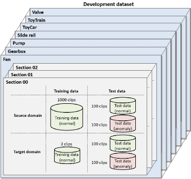
Figure 4: An overview of the development set of ASD [59].

IV-D2 Experimental setups

Log Mel spectrograms are used as input features for ASD models. The recordings are loaded with the default sample rate of 16,000Hz. We applied STFT with a Hanning window size of 1,024 and a hop length of 512 samples. Mel-filters with bands of 128 are used to generate log Mel spectrograms. In addition, the input features are obtained by concatenating consecutive 64 frames of the log Mel spectrograms. The final shape of the input to the network is $64\times 128$. The other setups are the same as described in Sec. IV-B2.

IV-D3 Baseline models

There are also three types of baseline models for ASD. The official baseline of DCASE 2021 Task2 is a MobileNetV2-based model [11]. This model is trained in a self-supervised manner using the IDs of the machines. Besides the official baseline model, the remaining two types of models (CNN5, CNN9, CNN13, and CNN-biGRU-Avg) are the same as described in Sec. IV-B3

IV-D4 Evaluation metrics

This task is evaluated with the area under the curve (AUC) of the receiver operating characteristic (ROC). We first define the anomaly score $A(\mathbf{X})$ as:

$$A(\mathbf{X}) =\operatorname{log}(\frac{1-f(\mathbf{X})}{f(\mathbf{X})})$$ (21)

$$=\frac{1}{B}\sum_{b=1}^{B}\operatorname{log}(\frac{1-f(\mathbf{X}_{b})}{f(\mathbf{X}_{b})})$$

$$=\frac{1}{B}\sum_{b=1}^{B}\operatorname{log}(\frac{1-\hat{y}_{b}}{\hat{y}_{b}}),$$

where $B$ is the number of the input features extracted from log Mel spectrograms by shifting a context window by $8$ frames, and $\hat{y}_{b}$ is the softmax output of the network. The AUC can be defined as:

$$\text{AUC}=\frac{1}{N_{-}N_{+}}\sum_{i=1}^{N_{-}}\sum_{j=1}^{N_{+}}\mathcal{H}(A(\mathbf{X}_{j}^{+})-A(\mathbf{X}_{i}^{-})),$$ (22)

where $\mathbf{X}_{j}^{+}$ and $\mathbf{X}_{i}^{-}$ are normal and anomalous test input features, $N_{+}$ and $N_{-}$ are the number of normal and anomalous test samples, respectively. And $\mathcal{H}(x)$ returns 1 when $x>0$ and 0 otherwise. Moreover, the partial-AUC (pAUC) is used as an additional metric, which is calculated from a portion of ROC over the pre-specified range of interest. In this task, the pAUC is calculated as the AUC over a low false-positive-rate (FPR) range [0,p], where we will use $p=0.1$.

V Results and discussions

In this section, we demonstrate the results of the experiments and give further discussions about the models from two aspects: cross-task, where the generality is analyzed, and subtask, where the individuality is analyzed. In addition, we visualize the attention masks of the proposed SE-Trans to study the effectiveness of the attention mechanism.

V-A Cross-task

For the cross-task aspect, we compare the general performance of the proposed cross-task model with other baseline models, and further investigate the importance of SE, Transformer modules, and data augmentation methods in our model.

V-A1 Comparison of different models

TABLE II: Cross-task performance comparison with different models.

Models	ASC	UST			ASD
	macro-ACC	macro-AUPRC	micro-AUPRC	micro-F1	AUC	pAUC
Official baseline [55] [56] [11]	0.477	0.632	0.835	0.739	0.622	0.574
CNN5 [28]	0.525	0.683	0.860	0.766	0.686	0.613
CNN9 [28]	0.550	0.678	0.862	0.767	0.703	0.616
CNN13 [28]	0.475	0.675	0.851	0.736	0.708	0.612
CNN-biGRU-Avg [31]	0.572	0.684	0.845	0.763	0.711	0.617
Proposed	0.633	0.727	0.872	0.785	0.751	0.632

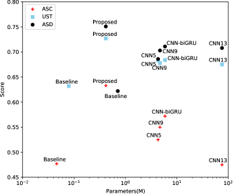
Figure 5: Parameters versus scores of different models. Official baseline (Baseline), CNN-biGRU-Avg (CNN-biGRU).

In this section, we compare the proposed cross-task model with state-of-the-art methods on different tasks, i.e., ASC, UST, and ASD. Table II shows that the proposed cross-task model surpasses the performance of official baselines, CNN5, CNN9, CNN13, and CNN-biGRU-Avg on all evaluation metrics. For ASC, the proposed model achieves a macro-ACC of 0.633; for UST, our model achieves a macro-AUPRC of 0.727, a micro-AUPRC of 0.872, and a micro-F1 of 0.785; for ASD, the proposed model achieves AUC and pAUC of 0.751 and 0.632, respectively.

In real applications, the number of parameters and performance has to be considered and there must be a trade-off between them. Therefore, we further analyzed the model complexity of the aforementioned models. Fig. 5 shows the parameters versus scores of different models for ASC, UST, and ASD, while the score used for comparison on each task is macro-ACC, macro-AUPRC, and AUC. As shown in the figure, CNN-biGRU-Avg performs better than the official baseline models, CNN5, CNN9, and CNN13 for all tasks, containing about 5.8 million parameters. The proposed cross-task model has achieved significant improvement and outperforms the models under comparison for all tasks. However, our model contains around 0.4 million parameters, which are only 7% of the model complexity of CNN-biGRU-Avg.

V-A2 Analysis of SE and Transformer modules

To further study the effectiveness of the Transformer encoder and SE modules, ablation experiments have been performed. Table III compares three different architectures with different numbers of CNN channels and blocks, and macro-ACC, macro-AUPRC, and AUC are implemented as evaluation measurements for ASC, UST, and ASD. CNN9 contains 4 CNN blocks with different numbers of channels, while CNN4-Trans contains 2 CNN blocks followed by a Transformer encoder. Then each CNN block in CNN4-Trans is replaced by an SE-block to get SE-Trans. For ASC, the CNN4-Trans achieves a macro-ACC of 0.589, outperforming the CNN9 by 7%. The SE-Trans further improves the macro-ACC of CNN4-Trans from 0.589 to 0.609. For UST, the performance of CNN4-Trans remains the same as macro-AUPRC of 0.678 with CNN9. SE-Trans achieves a macro-AUPRC of 0.699, outperforming the other networks. For ASD, the CNN4-Trans obtains an improvement of 0.008 in AUC and the SE-Trans obtains a further improvement of 0.009 in AUC. To summarize, both of the SE and Transformer modules improve the performance. The main reasons are that the channel-wise attention in SE layers and the MHSA in Transformer encoder can improve the performance of classifying similar acoustic scenes, tagging various urban sounds and detecting anomalous machines. Nevertheless, the contribution of these two modules varies for different tasks. The CNN4-Trans benefits much from the Transformer encoder for ASC, the SE-Trans achieves greater performance compared to CNN4-Trans for UST, both the Transformer encoder and SE layers can greatly improve the ASD performance.

TABLE III: Results of ablation experiments of SE and Transformer modules.

Network	Channels	ASC	UST	ASD
		macro-ACC	macro-AUPRC	AUC
CNN9	64/128/256/512	0.550	0.678	0.703
CNN4-Trans	64/128	0.589	0.678	0.712
SE-Trans	64/128	0.609	0.699	0.721

V-A3 Setups of Transformer encoder

We explored the importance of different numbers of layers, heads, and nodes of FFN in the Transformer encoder. Table IV shows the performance of SE-Trans for all the tasks using different numbers of head, layers, and nodes of FFN. For ASC, the best performance is achieved by the configuration of 1 layer, 8 heads, and 16 (or 32) nodes of FFN. For UST, the best number of layers, heads, and nodes of FFN is 1, 8, and 32, respectively. For ASD, the same configuration of 1 layer, 8 heads, and 32 nodes of FFN achieves the best AUC in comparison. Considering the performance of different configurations across these tasks, more layers do not achieve any benefit, and the number of heads and nodes of FFN should be chosen carefully. The combination of 1 layer, 8 heads, and 32 nodes of FFN can be considered as a proper choice for the proposed cross-task model.

TABLE IV: Performance of SE-Trans using different numbers of head, layers and nodes of FFN.

Layers	Heads	FFN	ASC	UST	ASD
			macro-ACC	macro-AUPRC	AUC
1	8	32	0.609	0.699	0.721
2	8	32	0.592	0.683	0.713
1	4	32	0.602	0.697	0.720
1	8	16	0.609	0.682	0.718
1	8	64	0.607	0.687	0.710

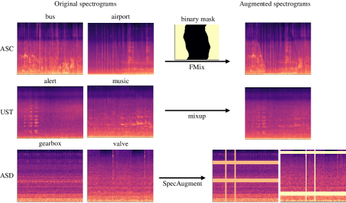
Figure 6: Examples of spectrograms augmented by SpecAugment, mixup and FMix for ASC, UST and ASD.

V-A4 Results of data augmentation methods

In this section, we investigate the performance of using different data augmentation methods: SpecAugment, mixup, and FMix. Comparative experiments are conducted on the proposed SE-Trans, and the experimental results are shown in Table V. For ASC, FMix improves the macro-ACC from 0.609 to 0.633, outperforming SpecAugment and mixup. For UST, FMix and mixup achieves an improvement of 0.022 and 0.028 on macro-AUPRC respectively, but applying SpecAugment does not improve the performance of UST. For ASD, FMix has significantly improved the AUC from 0.721 to 0.751, outperforming the comparative methods by a large margin. However, SpecAugment brings a slight reduction on the AUC score. We assume that SpecAugment is not suitable for different ESR tasks, because some key parts of the time-frequency features are randomly masked.

To further analyze, the examples of spectrograms augmented by SpecAugment, mixup and FMix for the tasks are shown in Fig. 6. In the left panel in Fig. 6, the spectrograms are examples of ASC, UST, and ASD, and the augmented spectrograms are listed in the right panel. FMix mixes two spectrograms by applying an irregular binary mask, which can generate a more complex spectrogram than mixup. Therefore, the model can learn robust acoustic features from the irregular areas on the complex spectrograms. SpecAugment partially masks time-frequency information by randomly setting columns and rows of the spectrograms to zero. This is effective for speech recognition, because the voice features can not be fully covered. However, some key acoustic information can be covered for ESR tasks. Considering the characteristics of environmental sound, SpecAugment should be carefully applied to ESR tasks.

TABLE V: Results of ablation experiments of data augmentation methods.

Data aug.	ASC	UST	ASD
	macro-ACC	macro-AUPRC	AUC
-	0.609	0.699	0.721
SpecAugment	0.607	0.701	0.717
mixup	0.613	0.721	0.727
FMix	0.633	0.727	0.751

V-B Subtask

For the subtask aspect, we further illustrate the performance of the proposed model on individual tasks.

V-B1 Analysis of acoustic scene classification

To further study the aforementioned contribution of Transformer and SE modules for ASC in Sec. V-A2, the confusion matrices achieved by CNN9, CNN4-Trans, and SE-Trans are shown in Fig. 7. CNN4-Trans and SE-Trans perform better than CNN9 for most of the classes, and the contribution of Transformer and SE modules can be illustrated by analyzing similar acoustic scenes. For example, the similar transportation scenes: bus, metro, and tram, are better classified; the performance of recognizing two open and outdoor scenes: park and public square, has been improved as well. The above observations verify that the attention mechanism in the Transformer encoder and SE layers can improve the performance of classifying similar scenes. Furthermore, some classes are not truly predicted, such as airport and street pedestrian. Since these scenes contain strong background noise and interference of human speech.

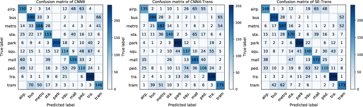
Figure 7: Confusion matrices of CNN9, CNN4-Trans and SE-Trans for ASC. Airport (airp.), shopping mall (mall), metro station (sta.), street pedestrian (ped.), public square (squ.), street traffic (tra.).

V-B2 Analysis of urban sound tagging

We investigate the class-wise performance of UST using different MSDA methods in this section. First of all, Fig. 8 shows the number of recordings of 8 coarse-level urban sound categories. The SONYC-UST-V2 dataset is imbalanced and the amounts of non-M/C, saw, music, and dog are less than other categories. These urban sound classes benefit from applying mixup or FMix, especially for music and dog. We assume that MSDA methods indeed generate more effective samples, which can help the model learn robust acoustic features and improve the classification performance especially for classes with fewer samples.

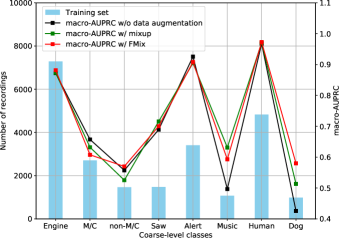
Figure 8: The number of recordings of 8 coarse-level urban sound categories and class-wise macro-AUPRC with different data augmentation methods. With (w/), without (w/o).

V-B3 Analysis of anomalous sound detection

In Sec. V-A4, we have shown some examples of spectrograms and analyzed the cross-task performance of different data augmentation methods. In this section, we compare the performance of ASD using FMix and SpecAugment, and the ROC curves of different machine types are illustrated in Fig. 9. As shown in Fig. 9, FMix performs the best for most of the machine types, where the anomalous sounds of toyCar, toyTrain, and fan can be correctly detected. These sounds have continuous acoustic characteristics, indicating that FMix can improve the performance of these machines. The performance achieved by SpecAugment is relatively poor on many machine types. This can verify the assumption in Sec. V-A4 that some key acoustic features on the spectrograms are randomly covered while applying SpecAugment.

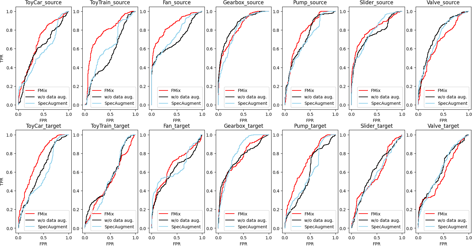
Figure 9: ROC curves of different machine types with different data augmentation methods. Without data augmentation (w/o data aug.), source domain (source), target domain (target).

V-C Visualization

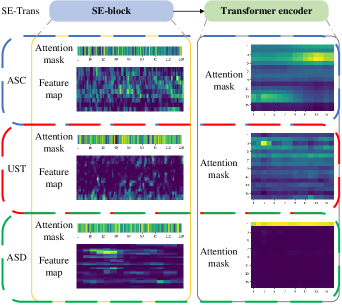
Figure 10: Visualization of attention masks on ASC, UST and ASD.

To study the effectiveness of the attention mechanism in the proposed SE-Trans, we further visualize the attention masks of the SE and Transformer encoder modules on ASC, UST, and ASD. The attention mask of SE is the channel-wise weighted vector $\mathbf{w}$ in Eq. 2 and Fig. 2, while the attention mask of the Transformer encoder is the mean attention of all the heads ($head_{i}$) in MHSA. Moreover, we show the most important feature map from all of the feature maps in the second SE-block, i.e., the maximum value of the channel-wise weighted vector $\mathbf{w}$. The attention masks and feature maps are shown in Fig. 10.

In Fig. 10, the attention masks of SE modules on different tasks are not the same. Specifically, the attention mask and feature map of ASC show that the feature map with global patterns is more important. For UST, the feature map shows more local but less global patterns. While for ASD, attention is paid more to local patterns. It is indicated that the global environmental background is meaningful for ASC task, the combination of different sounds is critical for UST, and the individual acoustic pattern is important for ASD.

For the attention mask of Transformer encoder, we can see that the relationship between temporal frames is different in the three tasks. The attention mask of ASC tends to model the temporal dependencies on most of the frames. While the attention mask of UST pays more attention to the dependencies on some of the frames. As for the attention mask of ASD, the attention is focused on a certain frame.

The visualization of attention masks illustrates distinct patterns for ASC, UST, and ASD tasks. It can be interpreted that the introduced attention mechanisms of SE and Transformer are effective to improve the performance of cross-task models for ESR.

VI Conclusion

This paper proposes a cross-task model to generally model acoustic knowledge across three different tasks of ESR. In the model, an architecture based on two types of attention mechanisms is presented, namely SE-Trans. This architecture exploits SE and Transformer encoder modules to learn the channel-wise importance and long sequence dependencies of the acoustic features. We also adopt FMix to augment training data and extract robust sound representations efficiently. Experiments show that our proposed cross-task model achieves state-of-the-art performance for ASC, UST, and ASD with lower computational resource demand. Further analysis and visualization experiments explore the generality and individuality of acoustic modeling for ESR, and illustrate the effectiveness and robustness of the proposed model.

Jisheng Bai received the B.S. degree in Detection Guidance and Control Technology from North University of China in 2017. He received the M.S. degree in Electronics and Communications Engineering from Northwestern Polytechnical University in 2020, where he is pursuing the Ph.D. degree. His research interests are focused on deep learning and environmental signal processing.

Jianfeng Chen received the Ph.D. degree in 1999, from Northwestern Polytechnical University. From 1999 to 2001, he was a Research Fellow in School of EEE, Nanyang Technological University, Singapore. During 2001-2003, he was with Center for Signal Processing, NSTB, Singapore, as a Research Scientist. From 2003 to 2007, he was a Research Scientist in Institute for Infocomm Research, Singapore. Since 2007, he works in College of Marine as a professor in Northwestern Polytechnical University, Xi’an, China. His main research interests include autonomous underwater vehicle design and application, array processing, acoustic signal processing, target detection and localization.

Mou Wang (Student Member, IEEE) received the B.S. degree in electronics and information engineering from Northwestern Polytechnical University, China, in 2016, where he is pursuing the Ph.D. degree in information and communication engineering. His research interests include machine learning and speech signal processing. He was awarded Outstanding Reviewer of IEEE Transactions on Multimedia.

Muhammad Saad Ayub received his B.E and M.Sc. degrees in 2010 and 2015 from National Univ. of Science and Technology Pakistan. He is currently working towards his PhD degree in School of Marine Science and Technology, Northwestern Polytechnical University, Xian. His research interests include acoustic signal analysis, multiple target localization, distributed acoustic networks, deep neural networks and formal analysis.

Qingli Yan received her Master’s degree and Ph.D. degree in signal processing from Northwestern Polytechnical University in 2015 and 2019. Since 2019, she has been a lecturer in the School of Computer Science & Technology, Xi’an University of Posts & Telecommunications. Her research interests include wireless sensor network, target localization and tracking.

References

- [1] K. Phua, J. Chen, T. H. Dat, and L. Shue, “Heart sound as a biometric,” Pattern Recognition, vol. 41, no. 3, pp. 906–919, 2008.
- [2] C.-F. Chan and E. W. M. Yu, “An abnormal sound detection and classification system for surveillance applications,” in 2010 18th European Signal Processing Conference, 2010, pp. 1851–1855.
- [3] G. Deshpande, A. Batliner, and B. W. Schuller, “Ai-based human audio processing for covid-19: A comprehensive overview,” Pattern Recognition, vol. 122, p. 108289, 2022.
- [4] R. Torres, D. Battaglino, and L. Lepauloux, “Baby cry sound detection: A comparison of hand crafted features and deep learning approach,” in International Conference on Engineering Applications of Neural Networks. Springer, 2017, pp. 168–179.
- [5] M. Asada, “Modeling early vocal development through infant–caregiver interaction: A review,” IEEE Transactions on Cognitive and Developmental Systems, vol. 8, no. 2, pp. 128–138, 2016.
- [6] A. Jan, H. Meng, Y. F. B. A. Gaus, and F. Zhang, “Artificial intelligent system for automatic depression level analysis through visual and vocal expressions,” IEEE Transactions on Cognitive and Developmental Systems, vol. 10, no. 3, pp. 668–680, 2017.
- [7] D. Stowell, D. Giannoulis, E. Benetos, M. Lagrange, and M. D. Plumbley, “Detection and classification of acoustic scenes and events,” IEEE Transactions on Multimedia, vol. 17, no. 10, pp. 1733–1746, 2015.
- [8] D. Barchiesi, D. Giannoulis, D. Stowell, and M. D. Plumbley, “Acoustic scene classification: Classifying environments from the sounds they produce,” IEEE Signal Processing Magazine, vol. 32, no. 3, pp. 16–34, 2015.
- [9] M. Cartwright, J. Cramer, A. E. M. Mendez, Y. Wang, H.-H. Wu, V. Lostanlen, M. Fuentes, G. Dove, C. Mydlarz, J. Salamon et al., “Sonyc-ust-v2: An urban sound tagging dataset with spatiotemporal context,” arXiv preprint arXiv:2009.05188, 2020.
- [10] J. Bai, J. Chen, and M. Wang, “Multimodal urban sound tagging with spatiotemporal context,” IEEE Transactions on Cognitive and Developmental Systems, 2022.
- [11] Y. Kawaguchi, K. Imoto, and Y. Koizumi, “Description and discussion on dcase 2021 challenge task2: unsupervised anomalous sound detection for machine condition monitoring under domain shifted conditions,” DCASE2021 Challenge, Tech. Rep., July 2021.
- [12] A. Mesaros, T. Heittola, E. Benetos, P. Foster, M. Lagrange, T. Virtanen, and M. D. Plumbley, “Detection and classification of acoustic scenes and events: Outcome of the dcase 2016 challenge,” IEEE/ACM Transactions on Audio, Speech, and Language Processing, vol. 26, no. 2, pp. 379–393, 2018.
- [13] T. Virtanen, M. D. Plumbley, and D. Ellis, Computational analysis of sound scenes and events. Springer, 2018.
- [14] A. Mesaros, T. Heittola, T. Virtanen, and M. D. Plumbley, “Sound event detection: A tutorial,” IEEE Signal Processing Magazine, vol. 38, no. 5, pp. 67–83, 2021.
- [15] M. Baelde, C. Biernacki, and R. Greff, “Real-time monophonic and polyphonic audio classification from power spectra,” Pattern Recognition, vol. 92, pp. 82–92, 2019.
- [16] M. A. Alamir, “A novel acoustic scene classification model using the late fusion of convolutional neural networks and different ensemble classifiers,” Applied Acoustics, vol. 175, p. 107829, 2021.
- [17] C. Szegedy, V. Vanhoucke, S. Ioffe, J. Shlens, and Z. Wojna, “Rethinking the inception architecture for computer vision,” in Proceedings of the IEEE conference on computer vision and pattern recognition, 2016, pp. 2818–2826.
- [18] Y. Luo and N. Mesgarani, “Conv-tasnet: Surpassing ideal time–frequency magnitude masking for speech separation,” IEEE/ACM transactions on audio, speech, and language processing, vol. 27, no. 8, pp. 1256–1266, 2019.
- [19] I. Sutskever, O. Vinyals, and Q. V. Le, “Sequence to sequence learning with neural networks,” in Advances in neural information processing systems, 2014, pp. 3104–3112.
- [20] M. Wang, M. Zhao, J. Chen, and S. Rahardja, “Nonlinear unmixing of hyperspectral data via deep autoencoder networks,” IEEE Geoscience and Remote Sensing Letters, vol. 16, no. 9, pp. 1467–1471, 2019.
- [21] J. Chen, M. Wang, X.-L. Zhang, Z. Huang, and S. Rahardja, “End-to-end multi-modal speech recognition with air and bone conducted speech,” in ICASSP 2022 - 2022 IEEE International Conference on Acoustics, Speech and Signal Processing (ICASSP), 2022, pp. 6052–6056.
- [22] L. Vuegen, B. Broeck, P. Karsmakers, J. F. Gemmeke, B. Vanrumste, and H. Hamme, “An mfcc-gmm approach for event detection and classification,” in IEEE Workshop on Applications of Signal Processing to Audio and Acoustics (WASPAA), 2013, pp. 1–3.
- [23] B. Uzkent, B. D. Barkana, and H. Cevikalp, “Non-speech environmental sound classification using svms with a new set of features,” International Journal of Innovative Computing, Information and Control, vol. 8, no. 5, pp. 3511–3524, 2012.
- [24] Z. Mushtaq, S.-F. Su, and Q.-V. Tran, “Spectral images based environmental sound classification using cnn with meaningful data augmentation,” Applied Acoustics, vol. 172, p. 107581, 2021.
- [25] J. Devlin, M.-W. Chang, K. Lee, and K. N. Toutanova, “Bert: Pre-training of deep bidirectional transformers for language understanding,” 2018.
- [26] A. Dosovitskiy, L. Beyer, A. Kolesnikov, D. Weissenborn, X. Zhai, T. Unterthiner, M. Dehghani, M. Minderer, G. Heigold, S. Gelly, J. Uszkoreit, and N. Houlsby, “An image is worth 16x16 words: Transformers for image recognition at scale,” in International Conference on Learning Representations, 2021.
- [27] Q. Kong, Y. Cao, T. Iqbal, Y. Wang, W. Wang, and M. D. Plumbley, “Panns: Large-scale pretrained audio neural networks for audio pattern recognition,” IEEE/ACM Transactions on Audio, Speech, and Language Processing, vol. 28, pp. 2880–2894, 2020.
- [28] Q. Kong, Y. Cao, T. Iqbal, W. Wang, and M. D. Plumbley, “Cross-task learning for audio tagging, sound event detection and spatial localization: DCASE 2019 baseline systems,” DCASE2019 Challenge, Tech. Rep., June 2019.
- [29] P. Jiang, X. Xu, H. Tao, L. Zhao, and C. Zou, “Convolutional-recurrent neural networks with multiple attention mechanisms for speech emotion recognition,” IEEE Transactions on Cognitive and Developmental Systems, 2021.
- [30] Z. Zhang, S. Xu, S. Zhang, T. Qiao, and S. Cao, “Attention based convolutional recurrent neural network for environmental sound classification,” Neurocomputing, vol. 453, pp. 896–903, 2021.
- [31] Q. Kong, Y. Xu, W. Wang, and M. D. Plumbley, “Sound event detection of weakly labelled data with cnn-transformer and automatic threshold optimization,” IEEE/ACM Transactions on Audio, Speech, and Language Processing, vol. 28, pp. 2450–2460, 2020.
- [32] Z. Ren, Q. Kong, K. Qian, M. D. Plumbley, B. Schuller et al., “Attention-based convolutional neural networks for acoustic scene classification,” in DCASE 2018 Workshop Proceedings, 2018.
- [33] J. Hu, L. Shen, and G. Sun, “Squeeze-and-excitation networks,” in Proceedings of the IEEE conference on computer vision and pattern recognition, 2018, pp. 7132–7141.
- [34] A. Harma, J. Jakka, M. Tikander, M. Karjalainen, T. Lokki, and H. Nironen, “Techniques and applications of wearable augmented reality audio,” in Audio Engineering Society Convention 114. Audio Engineering Society, 2003.
- [35] E. Martinson and A. Schultz, “Robotic discovery of the auditory scene,” in Proceedings 2007 IEEE International Conference on Robotics and Automation. IEEE, 2007, pp. 435–440.
- [36] A. Mesaros, T. Heittola, and T. Virtanen, “Acoustic scene classification: an overview of dcase 2017 challenge entries,” in 2018 16th International Workshop on Acoustic Signal Enhancement (IWAENC). IEEE, 2018, pp. 411–415.
- [37] H. Chen, Z. Liu, Z. Liu, P. Zhang, and Y. Yan, “Integrating the data augmentation scheme with various classifiers for acoustic scene modeling,” DCASE2019 Challenge, Tech. Rep., June 2019.
- [38] S. Suh, S. Park, Y. Jeong, and T. Lee, “Designing acoustic scene classification models with CNN variants,” DCASE2020 Challenge, Tech. Rep., June 2020.
- [39] J. P. Bello, C. Silva, O. Nov, R. L. Dubois, A. Arora, J. Salamon, C. Mydlarz, and H. Doraiswamy, “Sonyc: A system for monitoring, analyzing, and mitigating urban noise pollution,” Communications of the ACM, vol. 62, no. 2, pp. 68–77, Feb 2019.
- [40] S. Adapa, “Urban sound tagging using convolutional neural networks,” DCASE2019 Challenge, Tech. Rep., September 2019.
- [41] T. Iqbal, Y. Cao, M. D. Plumbley, and W. Wang, “Incorporating auxiliary data for urban sound tagging,” DCASE2020 Challenge, Tech. Rep., October 2020.
- [42] Y. Koizumi, Y. Kawaguchi, K. Imoto, T. Nakamura, Y. Nikaido, R. Tanabe, H. Purohit, K. Suefusa, T. Endo, M. Yasuda, and N. Harada, “Description and discussion on DCASE2020 challenge task2: Unsupervised anomalous sound detection for machine condition monitoring,” in Proceedings of the Detection and Classification of Acoustic Scenes and Events 2020 Workshop (DCASE2020), November 2020, pp. 81–85.
- [43] K. Dohi, T. Endo, H. Purohit, R. Tanabe, and Y. Kawaguchi, “Flow-based self-supervised density estimation for anomalous sound detection,” in ICASSP 2021-2021 IEEE International Conference on Acoustics, Speech and Signal Processing (ICASSP). IEEE, 2021, pp. 336–340.
- [44] K. Morita, T. Yano, and K. Tran, “Anomalous sound detection using cnn-based features by self supervised learning,” DCASE2021 Challenge, Tech. Rep., July 2021.
- [45] Q. Kong, I. Sobieraj, W. Wang, and M. Plumbley, “Deep neural network baseline for DCASE challenge 2016,” DCASE2016 Challenge, Tech. Rep., September 2016.
- [46] Q. Kong, I. Turab, X. Yong, W. Wang, and M. D. Plumbley, “DCASE 2018 challenge surrey cross-task convolutional neural network baseline,” DCASE2018 Challenge, Tech. Rep., September 2018.
- [47] S. Chaudhari, V. Mithal, G. Polatkan, and R. Ramanath, “An attentive survey of attention models,” ACM Transactions on Intelligent Systems and Technology (TIST), vol. 12, no. 5, pp. 1–32, 2021.
- [48] A. Gulati, J. Qin, C.-C. Chiu, N. Parmar, Y. Zhang, J. Yu, W. Han, S. Wang, Z. Zhang, Y. Wu, and R. Pang, “Conformer: Convolution-augmented Transformer for Speech Recognition,” in Proc. Interspeech 2020, 2020, pp. 5036–5040. [Online]. Available: http://dx.doi.org/10.21437/Interspeech.2020-3015
- [49] T. DeVries and G. W. Taylor, “Improved regularization of convolutional neural networks with cutout,” arXiv preprint arXiv:1708.04552, 2017.
- [50] D. S. Park, W. Chan, Y. Zhang, C.-C. Chiu, B. Zoph, E. D. Cubuk, and Q. V. Le, “SpecAugment: A Simple Data Augmentation Method for Automatic Speech Recognition,” in Proc. Interspeech 2019, 2019, pp. 2613–2617.
- [51] H. Zhang, M. Cisse, Y. N. Dauphin, and D. Lopez-Paz, “mixup: Beyond empirical risk minimization,” in International Conference on Learning Representations, 2018.
- [52] E. Harris, A. Marcu, M. Painter, M. Niranjan, A. Prugel-Bennett, and J. Hare, “{FM}ix: Enhancing mixed sample data augmentation,” 2021. [Online]. Available: https://openreview.net/forum?id=oev4KdikGjy
- [53] J. L. Ba, J. R. Kiros, and G. E. Hinton, “Layer normalization,” arXiv preprint arXiv:1607.06450, 2016.
- [54] T. Heittola, A. Mesaros, and T. Virtanen, “Acoustic scene classification in dcase 2020 challenge: generalization across devices and low complexity solutions,” in Proceedings of the Detection and Classification of Acoustic Scenes and Events 2020 Workshop (DCASE2020), 2020, pp. 56–60.
- [55] I. Martín-Morató, T. Heittola, A. Mesaros, and T. Virtanen, “Low-complexity acoustic scene classification for multi-device audio: analysis of dcase 2021 challenge systems,” 2021.
- [56] M. Cartwright, A. E. M. Mendez, J. Cramer, V. Lostanlen, G. Dove, H.-H. Wu, J. Salamon, O. Nov, and J. Bello, “SONYC urban sound tagging (SONYC-UST): A multilabel dataset from an urban acoustic sensor network,” in Proceedings of the Workshop on Detection and Classification of Acoustic Scenes and Events (DCASE), October 2019, pp. 35–39.
- [57] R. Tanabe, H. Purohit, K. Dohi, T. Endo, Y. Nikaido, T. Nakamura, and Y. Kawaguchi, “MIMII DUE: Sound dataset for malfunctioning industrial machine investigation and inspection with domain shifts due to changes in operational and environmental conditions,” In arXiv e-prints: 2006.05822, 1–4, 2021.
- [58] N. Harada, D. Niizumi, D. Takeuchi, Y. Ohishi, M. Yasuda, and S. Saito, “ToyADMOS2: Another dataset of miniature-machine operating sounds for anomalous sound detection under domain shift conditions,” arXiv preprint arXiv:2106.02369, 2021.
- [59] “Dcase 2021 task 2,” https://dcase.community/challenge2021/task-unsupervised-detection-of-anomalous-sounds.