Abstract

Datacenters execute large computational jobs, which are composed of smaller tasks. A job completes when all its tasks finish, so stragglers—rare, yet extremely slow tasks—are a major impediment to datacenter performance. Accurately predicting stragglers would enable proactive intervention, allowing datacenter operators to mitigate stragglers before they delay a job. While much prior work applies machine learning to predict computer system performance, these approaches rely on complete labels—i.e., sufficient examples of all possible behaviors, including straggling and non-straggling—or strong assumptions about the underlying latency distributions—e.g., whether Gaussian or not. Within a running job, however, none of this information is available until stragglers have revealed themselves when they have already delayed the job. To predict stragglers accurately and early without labeled positive examples or assumptions on latency distributions, this paper presents Nurd, a novel Negative-Unlabeled learning approach with Reweighting and Distribution-compensation that only trains on negative and unlabeled streaming data. The key idea is to train a predictor using finished tasks of non-stragglers to predict latency for unlabeled running tasks, and then reweight each unlabeled task’s prediction based on a weighting function of its feature space. We evaluate Nurd on two production traces from Google and Alibaba, and find that compared to the best baseline approach, Nurd produces 2–11 percentage point increases in the F1 score in terms of prediction accuracy, and 2.0–8.8 percentage point improvements in job completion time.

1 Introduction

Stragglers impede job completion in datacenter-scale computing. Here, a computational job is split into many tasks, each of which is executed in parallel on different machines before their results are aggregated when the last task completes. Stragglers are rare, extremely slow tasks within a job that can degrade overall performance—by as much as 30–50% Ananthanarayanan et al. (2013); Reiss et al. (2011); Zheng & Lee (2018). A straggler is commonly defined as a task with at least 90th percentile (p90) latency; i.e., at least 90% of tasks finish earlier than the straggler Hao et al. (2017; 2020). We refer to stragglers as the positive class since they are the minority and abnormal, and non-stragglers are the negative class since they are the majority and expected Chandola et al. (2009).

Mitigating stragglers is a fundamental problem in datacenters Zhou et al. (2021); Belay et al. (2014); Adya et al. (2016); Handley et al. (2017); Haque et al. (2015); Nelson et al. (2015); Ayers et al. (2019). Recent work uses predictive models to monitor executing tasks and predict stragglers before they reveal themselves with long run times Ananthanarayanan et al. (2010); Ren et al. (2015); Yadwadkar et al. (2014); Zhou et al. (2020). Once a straggler is correctly predicted, proactive interventions—such as relaunching the same task on a different machine—will be triggered to mitigate the straggling behavior Ananthanarayanan et al. (2013); Aktas et al. (2017); Aktas & Soljanin (2019). Machine learning techniques have been applied to model the complicated, nonlinear relationships between features (e.g., CPU utilization) and computation behavior (e.g., latency)—a recent survey has details Penney & Chen (2019). However, most existing work either heavily relies on complete labels—i.e., observing labeled samples from all classes at training—or strong assumptions about the underlying latency distribution—e.g., whether Gaussian or not. When predicting stragglers on live data—i.e., running jobs in the datacenter—stragglers are not revealed early because they finish last. Therefore, there are insufficient labels in the training set due to a lack of positive examples of stragglers, and it is hard to pre-specify the latency distribution for each job, which render most learning methods ineffective for straggler prediction within a running job. Moreover, since the characteristics of each job are usually unique in datacenters Reiss et al. (2012); Guo et al. (2019), it is difficult to train a model on one job and apply it to another directly. Therefore, this paper proposes a technique that constructs a unique predictive model for each job on the fly—that is, as the job is running and before stragglers reveal themselves with long completion time.

We present Nurd, a novel negative-unlabeled learning approach for online straggler prediction that requires no labeled positive examples or assumptions on the latency distributions. Nurd uses finished tasks (i.e., negative examples, non-stragglers) to train a model to predict latency as a function of observed task features for running tasks. Nurd’s key insight is that this predictor will be biased towards non-stragglers, so it then reweights these latency predictions using a function of task features—i.e., each running task’s probability of being included in the set of finished tasks given its observed features. Intuitively, this weighting function indicates how dissimilar a particular running task’s features are from those that are finished; i.e., it preserves latency predictions for tasks that are similar to finished tasks (i.e., non-stragglers), and increases predicted latency for those that are different. With this reweighting scheme, Nurd predicts stragglers early and accurately by reducing the prediction bias due to a lack of stragglers at training.

To summarize, our main contributions are as follows:

• We propose a novel negative-unlabeled learning approach based on reweighting predictions and demonstrate its efficacy for online straggler prediction when no labeled stragglers exist in the training set.

• We evaluate Nurd on Google production traces Reiss et al. (2011), where we observe an 11 percentage point increase in the F1 score and 3.8–8.8 percentage point improvement in job completion time relative to the best baseline approach. Similarly, on Alibaba production traces Alibaba , we see a 2 point increase in the F1 score and an 2.0–3.5 point improvement in job completion time.

• We release the code in https://github.com/y-ding/nurd-mlsys22-code.

Stragglers significantly hamper system performance in modern datacenters. By identifying stragglers accurately and early for running jobs, Nurd provides a novel online learning approach that does not require labeled positive examples of stragglers or assumptions on latency distributions. This work offers a new direction in which systems community can apply machine learning techniques that can generalize without heavy reliance on carefully curating training sets.

2 Background

Datacenter terminology. Datacenter-scale computations, or jobs, are composed of sub-computations called tasks. Because datacenter performance is critical, jobs are continually monitored and tasks’ behavior in a variety of metrics are recorded at regular time checkpoints Reiss et al. (2011; 2012). These recorded measurements are a set of features that characterize each task. The choice of metrics to monitor (and thus features to capture) depends on the specific system on which the job is deployed. Ideally, datacenters would record metrics related to resource usage, microarchitectural behavior, and job scheduling Zheng & Lee (2018). In such scenario, a straggler prediction algorithm could be applied at each checkpoint using the features from each task to predict its future latency. If a particular task is expected to straggle—i.e., exceed an operator-specified latency threshold—then the job scheduler or human operator could be alerted to trigger intervention to mitigate stragglers.

Straggler mitigation. Straggler mitigation is an important part of datacenter scheduling Dean & Barroso (2013); Schwarzkopf & Bailis (2018); Aktas & Soljanin (2019); Dean & Ghemawat (2004); Zaharia et al. (2008); Ananthanarayanan et al. (2011). Performance-aware schedulers predict which tasks are likely to straggle and then allocate additional resources to them Ananthanarayanan et al. (2010); Yadwadkar et al. (2014); Ren et al. (2015). Wrangler is a typical system like this, using linear support vector machines to classify stragglers by oversampling stragglers to deal with imbalanced labels in the training set Yadwadkar et al. (2014). Another example is LinnOS, which uses neural networks to predict anomalous I/O latency by training on tens of thousands of I/O operations from a single hardware device with known latency Hao et al. (2020). A clear limitation of these approaches is that they require positive examples of stragglers. To the best of our knowledge, prior performance-aware schedulers assume that they have access to at least some examples of stragglers to train a model. This is a strong assumption that does not hold if users develop new jobs that are different from existing jobs (which is the common case for datacenter jobs Reiss et al. (2012); Guo et al. (2019)) or if datacenters install new hardware that induces new causes of straggling behavior. Thus, there is a need for performance-aware scheduling approaches that produce accurate predictions without positive examples of stragglers.

Problem formulation. Given the above discussion, we formalize the online straggler prediction problem as follows. Imagine we have $T$ time checkpoints. At the $t$-th checkpoint where $t\in[T]$, $n$ tasks are observed for a job, and the $i$-th task is associated with a feature vector $x_{ti}\in\mathbb{R}^{d}$, where $d$ is the number of features (measurements) that characterize the task. Task $i$ has true latency $y_{i}\in\mathbb{R}_{+}$. Let $\tau^{\rm stra}$ denote the target latency threshold that denotes straggling (e.g., the p90 latency), and $S:=\{i\in[n]:y_{i}\geq\tau^{\rm stra}\}$ denote the set of tasks that are true stragglers. Our goal is to identify the straggler set $S$. The challenge is that we do not observe $y_{i}$ for all tasks at the $t$-th checkpoint. Rather, we only observe $y_{i}$ when $y_{i}\leq\tau_{t}^{\rm run}\leq\tau^{\rm stra}$, where $\tau_{t}^{\rm run}$ is the latency at $t$-th time checkpoint. Let $F_{t}:=\{i\in[n]:y_{i}\leq\tau_{t}^{\rm run}\}$ denote the tasks that finish before $t$-th time checkpoint, and $R_{t}$ be the list of tasks that are still running at the $t$-th time checkpoint. At each $t$-th checkpoint, given $x_{ti}$ for $i\in[n]$ and $y_{i}$ for $i\in F_{t}$, we estimate a set of stragglers $\hat{S}$ from the unfinished tasks at $\tau_{t}^{\rm run}$. Our goal is to correctly identify stragglers, so that intervention can occur as early as possible.

3 Related Work

We notice the following limitations from the existing approaches applied to online straggler prediction:

• Difficulty of accounting for the drift between training and test distribution (supervised learning in section 3.1).

• Only using information from the feature space and ignoring the observed latency (outlier detection in section 3.2).

• Incorrect independence assumptions on labels given features (PU learning in section 3.3).

• Heavy reliance on pre-specified latency distribution (censored and survival regression in section 3.4).

3.1 Supervised Learning

Supervised learning uses labeled samples to learn a predictor $h_{t}$ so that $\hat{y}_{ti}=h_{t}(x_{ti})$ for $i$-th task at $t$-th checkpoint; this predictor could estimate the latency of the unlabeled samples. Critically, however, the distribution of the unlabeled samples is different from that of the labeled samples; that is, the nature of the straggler prediction problem necessitates a distribution drift between training and prediction, and we must be robust to that drift. Without accounting for this drift, latency predictions for stragglers will be heavily biased Quiñonero-Candela et al. (2009); Zhang et al. (2013).

3.2 Outlier Detection (Unsupervised Learning)

Outlier—or anomaly—detection is a family of unsupervised learning techniques that identifies rare events which differ from the general distribution of a population Chandola et al. (2007); Alam et al. (2019); Sipple (2020). These techniques separate nominal and anomalous distributions based on the observations in the feature space only. Although stragglers can be thought of as outliers, our online straggler prediction problem is critically different from outlier detection problems studied in the literature because stragglers—by definition—are outliers in latency, which are not necessarily outliers in the feature space. As such, while we have access to each task’s features at $t$-th time checkpoint, their latency values are revealed only up to time $t$. To address the issue of only using information from feature space, Nurd proposes to reweight the predicted latency with a weighting function to reduce the prediction bias in latency due to a lack of stragglers at training. Empirically, we evaluate fourteen existing outlier detection methods in section 7 to demonstrate that outlier detection methods have limited discriminative power in identifying stragglers within running jobs.

3.3 PU Learning (Semi-supervised Learning)

Positive-unlabeled (PU) learning is a family of semi-supervised learning techniques that use both labeled and unlabeled samples to train a classifier Bekker & Davis (2020). PU learning approaches learn from the two sets of examples, where the first set (positive) only contains examples from the first class, while the other set (unlabeled) contains examples from both classes. Existing PU learning Lee & Liu (2003); Elkan & Noto (2008); Mordelet & Vert (2014); Kiryo et al. (2017) assumes that observations of the labels are independent of the features given the classes (positive or negative); that is, the labeled examples are a random sample from the positive examples. However, this assumption is violated in online straggler prediction because only some non-stragglers with lower latency values have a chance to be sampled, while other non-stragglers with higher latency values are not included in the labeled set.

3.4 Censored and Survival Regression

Censored regression is a family of techniques to handle the situation where the value to be predicted (latency in this case) is censored; i.e., some values are missing but known to exceed certain thresholds Powell (1986). Survival regression is a related field that predicts when a system will survive beyond a certain time point. The latency variable in the online straggler prediction problem can be viewed as being censored at each checkpoint $t$ because the latency values above $t$ are not revealed. There are both linear (Tobit Tobin (1958)) and non-linear (Grabit Sigrist & Hirnschall (2019)) methods for censored regression. The Cox proportional hazard (CoxPH) model is a popular approach for survival analysis Cox (1972). All three methods can be used to estimate latency with incomplete labels: latency can be viewed as being censored at each checkpoint $t$ because the latency values above $t$ are not revealed; alternatively, we could cast the problem as estimating whether a task will survive beyond the designated straggling latency. While the technical details of all three models differ greatly, they share a common assumption: that the underlying task latency behavior is known a priori. Tobit and Grabit assume the latency follows a Gaussian distribution, and they predict censored values according to this assumption. CoxPH makes a more relaxed assumption: rather than assuming a particular distribution, it assumes that all task’s transformed survival curves (survival probability over time) have the same shape Hosmer et al. (2008), an assumption that does not hold in the online straggler prediction problem as heterogeneous behavior (either in the tasks themselves or the machines executing those tasks) is a common cause of straggling. In addition, the CoxPH model assumes that the relationship between a task’s features and straggling behavior does not change over time, but this is not true in practice and Nurd explicitly accounts for this behavior (section 4.3).

3.5 Summary

To address all the issues from the existing approaches applied to online straggler prediction, we propose Nurd, a negative-unlabeled learning approach that requires no labeled positive examples of stragglers or assumptions on the latency distributions. Nurd incorporates a data-driven way to learn the weighting function from feature space that can easily adapt to different types of distributions. Specifically, Nurd uses the fact that unlabeled samples satisfy $y_{i}\geq\tau_{t}^{\rm run}$, rather than relying on any assumptions about the latency distribution. The next section describes how Nurd learns a weighting function based on task features to mitigate the bias of supervised learning on the labeled samples.

4 The proposed approach: Nurd

Nurd is a novel negative-unlabeled learning approach for online straggler prediction without positive examples at training or assumptions on latency distributions. Specifically, Nurd trains a new predictor for each job, customizing to that job’s unique properties. The key idea is to first train a latency predictor using only finished tasks (i.e., non-stragglers), and then reweight those latency predictions based on a function of dissimilarity between finished and running tasks from the feature space. Algorithm 1 summarizes Nurd. In particular, there are three key components:

1. Training with finished tasks (section 4.1).

2. Reweighting based on feature space (section 4.2).

3. Updating models online (section 4.3).

Next, we describe each in detail.

4.1 Training with Finished Tasks

Nurd starts by training a latency predictor using the labeled finished tasks (i.e., non-stragglers, or negative examples). While any regression model can be applied, Nurd uses gradient boosting trees due to its high predictive power in many settings Chen & Guestrin (2016). At the $t$-th time checkpoint for the $i$-th task, Nurd trains the regression model $h_{t}$ so that the predicted latency is $\hat{y}_{ti}=h_{t}(x_{ti})$. However, since it only trains on negative examples, the predictions will be heavily biased towards finished tasks (i.e., non-stragglers). To reduce such bias, Nurd reweights the predictions, leading to the next step.

4.2 Reweighting Based on Feature Space.

To reduce the bias from training on finished tasks only, Nurd reweights $\hat{y}_{ti}$. At the $t$-th time checkpoint for the $i$-th task, Nurd uses a weighting function $w_{ti}\in(0,1]$ such that

$$\hat{y}_{ti}^{\rm adj}=\frac{\hat{y}_{ti}}{w_{ti}},$$ (1)

where $\hat{y}_{ti}^{\rm adj}$ is the adjusted latency prediction for the $i$-th task. Intuitively, when a running task’s features are similar to finished tasks (i.e., non-stragglers), we want $w_{ti}$ to be relatively large (close to 1) such that $\hat{y}_{ti}^{\rm adj}$ does not change much from $\hat{y}_{ti}$. When a running task’s features are different from finished tasks, we want $w_{ti}$ to be relatively small (close to 0) such that $\hat{y}_{ti}^{\rm adj}$ will be enlarged and more likely to exceed the latency threshold and be classified as a straggler.

To find a weighting function that matches our intuition, Nurd uses propensity score (PS), which is defined as the conditional probability of assignment to a particular group given a set of observed features Rosenbaum & Rubin (1983). In our case, we denote $z_{ti}$ as PS; i.e., the conditional probability that a task belongs to the class of finished tasks given its features at time checkpoint $t$:

$$z_{ti}=\mathbb{P}(y_{i}\leq\tau_{t}^{\rm run}|x_{ti}).$$ (2)

In practice, $z_{ti}$ is usually estimated using logistic regression Cepeda et al. (2003) because we have two known classes at the $t$-th checkpoint: finished tasks and running tasks. When $z_{ti}$ has relatively higher probability value (close to 1), it indicates that the $i$-th task has higher chances that it will finish soon (i.e., a non-straggler), and thus using it to reweight $\hat{y}_{ti}$ will not cause a large change in the latency prediction. In contrast, when $z_{ti}$ has a relatively low probability value (close to 0), it indicates that the $i$-th task has a higher chance that it will keep running (i.e., straggle), and thus using it to reweight $\hat{y}_{ti}$ will dilate the latency prediction and make it more likely to exceed the latency threshold.

Algorithm 1 Online straggler prediction with Nurd.

Input: $T$: number of time checkpoints; $F_{0}$: list of tasks finished at initial checkpoint $t=0$; $R_{0}$: list of tasks running at initial checkpoint $t=0$; $\tau^{\rm stra}>0$: latency threshold; $\alpha>0$: calibration parameter; $\epsilon>0$: minimum positive weight.
Output: $\hat{S}$

1:  Initialize $X_{\mathrm{fin}}$ and $X_{\mathrm{run}}$ with features from tasks in $F_{0}$ and $R_{0}$, i.e., $X_{\mathrm{fin}}=\{x_{0i};i\in F_{0}\},X_{\mathrm{run}}=\{x_{0i};i\in R_{0}\}$.

2:  Initialize $Y_{\mathrm{fin}}$ in $F_{0}$, i.e., $Y_{\mathrm{fin}}=\{y_{i};i\in F_{0}\}$.

3:  Straggler set $\hat{S}\leftarrow\emptyset$.

4:  Compute centroids of $X_{\mathrm{fin}}$ and the rest running tasks $X_{\mathrm{run}}$, denoted as $c_{\mathrm{fin}}$ and $c_{\mathrm{run}}$.

5:  $\rho=\|c_{\mathrm{fin}}\|^{2}/\|c_{\mathrm{run}}-c_{\mathrm{fin}}\|^{2}$. $\lx@algorithmic@hfill\triangleright$ Compute latency indicator

6:  $\delta=\frac{1}{1+\rho}-\alpha$. $\lx@algorithmic@hfill\triangleright$ Compute calibration term

7:  for each time checkpoint $t=1,\ldots,T$ do

8:     $\Delta_{t}\leftarrow\{i\in R_{t-1};y_{i}\leq\tau_{t}^{\rm run}\}$. $\lx@algorithmic@hfill\triangleright$ Update tasks finished between $t-1$ and $t$-th checkpoint

9:     $F_{t}\leftarrow F_{t-1}\bigcup\Delta_{t}$, $R_{t}\leftarrow R_{t-1}\setminus\Delta_{t}$. $\lx@algorithmic@hfill\triangleright$ Update sets of finished and running tasks

10:     $X_{\mathrm{fin}}\leftarrow X_{\mathrm{fin}}\bigcup\{x_{ti};i\in\Delta_{t}\}$, $Y_{\mathrm{fin}}\leftarrow Y_{\mathrm{fin}}\bigcup\{y_{i};i\in\Delta_{t}\}$, and $X_{\mathrm{run}}\leftarrow\{x_{ti};i\in R_{t}\}$.

11:     Update latency prediction model $h_{t}$ and PS estimation model $g_{t}$ using updated $X_{\mathrm{fin}},Y_{\mathrm{fin}}$, and $X_{\mathrm{run}}$.

12:     for each task $i\in R_{t}$  do

13:        Get initial latency prediction $\hat{y}_{ti}=h_{t}(x_{ti})$.

14:        Get PS estimation $z_{ti}=g_{t}(x_{ti})$.

15:        $w_{ti}=\max(\epsilon,\min(z_{ti}+\delta,1))$ $\lx@algorithmic@hfill\triangleright$ Construct final weighting function

16:        Get adjusted latency prediction $\hat{y}_{ti}^{\rm adj}=\frac{\hat{y}_{ti}}{w_{ti}}$.

17:        if $\hat{y}_{ti}^{\rm adj}\geq\tau^{\rm stra}$ then

18:           $\hat{S}\leftarrow\hat{S}\bigcup\{i\}$, $R_{t}\leftarrow R_{t}\setminus\{i\}$ $\lx@algorithmic@hfill\triangleright$ Terminate the task $i$ if a straggler is predicted

19:  return $\hat{S}$

Algorithm 2 Scheduling with more machines than tasks.

Input: $T$: number of time checkpoints; $[n]$: set of running tasks

1:  for each time checkpoint $t\in[T]$ do

2:     for each running task $i\in[n]$ do

3:        if task $i$ is predicted to be a straggler then

4:           Terminate $i$ and relaunch it on a new machine.

5:           Update set of running tasks $[n]\leftarrow[n]\setminus\{i\}$.

6:        else

7:           Go to next task.

Algorithm 3 Scheduling with fewer machines than tasks.

Input: $T$: number of time checkpoints; $[n]$: set of running tasks; $[m]$: set of available machines.

1:  for each time checkpoint $t\in[T]$ do

2:     if new machine $k$ available then

3:        Update set of available machines $[m]\leftarrow[m]\bigcup\{k\}$.

4:     for each running task $i\in[n]$ do

5:        if task $i$ is predicted to be a straggler then

6:           if machines are available $[m]\neq\emptyset$  then

7:              Terminate $i$ and relaunch it on a new machine $j$.

8:              Update set of running tasks $[n]\leftarrow[n]\setminus\{i\}$.

9:              Update set of available machines $[m]\leftarrow[m]\setminus\{j\}$.

10:           else

11:              Go to next task.

Calibration. Different jobs have different latency distributions, and thus have different target latency thresholds to determine stragglers. To account for such difference, Nurd adds a calibration term $\delta$ to the propensity scores to construct the final weighting function and balance the tradeoffs between true and false positives. Specifically, this calibration term is a function of the latency threshold; i.e., whether the latency threshold (e.g. p90) is greater than the half of the maximum latency.

(a)

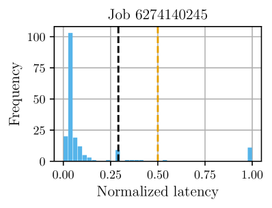
(b)

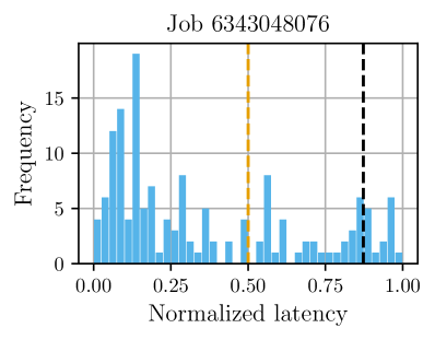
Figure 1: Latency distributions for two Google jobs. The vertical dashed yellow line is half of the maximum normalized latency 0.5, and the dashed black line is the latency threshold (e.g. p90).

• If the latency threshold is less than the half of the maximum latency (left side of Figure 1), the latency threshold is relatively small compared to the maximum latency. To reduce the false positives in predictions, we hope to increase the weighting value such that $\hat{y}_{ti}$ will not be enlarged too much. Therefore, $\delta$ should be relatively large but not exceed 1; i.e., $w_{ti}=\min(z_{ti}+\delta,1)$.

• If the latency threshold is greater than the half of the maximum latency (right side of Figure 1), the latency threshold is relatively large. To reduce the false negatives in predictions, we hope to decrease the weighting value such that $\hat{y}_{ti}$ will be enlarged enough. Therefore, $\delta$ should be relatively small but not make $w_{ti}$ negative; i.e., $w_{ti}=\max(\epsilon,\min(z_{ti}+\delta,1))$, where $\epsilon$ is a small positive scalar.

With this insight, we address the remaining questions as follows: (1) how to determine whether the latency threshold is relatively large or small when the job is still running (since the actual task latencies are unknown), and (2) how to set $\delta$.

Determining whether latency threshold is relatively large or small. As noted in section 3 prior work for outlier detection and censored regression assumes a distribution (almost always Gaussian) for the values (in this case latency) they are trying to predict. Such an assumption makes determining the relative size of the latency threshold trivial. A key distinction of Nurd is that it makes no such assumption (and Figure 1 shows that no single assumption would suffice). Specifically, Nurd estimates the relative magnitude of the latency threshold from tasks’ observed features, rather than from assumptions about the latency distribution. Inspired by the insight that running tasks’ features are different from those of finished tasks, Nurd compares the feature centroids of finished tasks (non-stragglers) $c_{\mathrm{fin}}$ and those of running tasks $c_{\mathrm{run}}$ before starting prediction. Empirically, Nurd computes $\rho=\|c_{\mathrm{fin}}\|^{2}/\|c_{\mathrm{run}}-c_{\mathrm{fin}}\|^{2}$.

The intuition is that $\rho$ indicates how far potential stragglers are from non-stragglers. If potential stragglers are far from non-stragglers (left side of Figure 1), $c_{\mathrm{run}}$ is likely to be far from $c_{\mathrm{fin}}$ and $\rho\leq 1$. In this case, the unweighted latency prediction $\hat{y}_{ti}$ is easily pushed over the threshold, which makes PS overcorrect the latency predictions. Therefore, increasing the weight by making $\delta$ relatively large has little effect on true positives, but decreases false positives. In contrast, if potential stragglers are close to non-stragglers (right side of Figure 1), $c_{\mathrm{run}}$ is likely to be close to $c_{\mathrm{fin}}$ and $\rho>1$. In this case, true stragglers may not be easily pushed over the threshold by $\hat{y}_{ti}$ because the features of all tasks are not so different, which makes PS alone not enough for reweighting. Therefore, reducing the weight by making $\delta$ relatively small increases the true positives significantly, despite a possible small increase in false positives.

Setting $\delta$. Assuming $\delta\in(-\alpha,\alpha)$, where $\alpha>0$. As discussed above, $\delta$ is a function of $\rho$. When the latency threshold is relatively small ($\rho\leq 1$), $\delta$ is relatively large. When the latency threshold is relatively large ($\rho>1$), $\delta$ is relatively small. Therefore, Nurd uses a function $f:\mathbb{R}_{+}\times\mathbb{R}\to(-\alpha,\alpha)$ such that $\delta=f(\rho,\alpha)$:

$$\delta=\frac{1}{1+\rho}-\alpha.$$ (3)

With $z_{ti}$, $\delta$, and $\hat{y}_{ti}$, Nurd obtains

$$\hat{y}_{ti}^{\rm adj}=\frac{\hat{y}_{ti}}{\max(\epsilon,\min(z_{ti}+\delta,1))}$$ (4)

Nurd identifies stragglers if $\hat{y}_{ti}^{\rm adj}\geq\tau^{\rm stra}$; i.e., the predicted latency exceeds the latency threshold. Since the exact value of $\tau^{\rm stra}$ is unknown a priori, it can either be selected manually by users or automatically by techniques such as those in LinnOS Hao et al. (2020) that estimate the inflection point in the latency CDF. Determining the latency threshold is beyond the scope of this work. Tests with a wide variety of thresholds show that Nurd produces results that are robust to the different latency thresholds.

4.3 Updating Models Online

As the job is running, Nurd accumulates examples of finished tasks at each checkpoint and Nurd uses these new examples to update both the latency predictor $h_{t}$ and propensity score model in Equation 2 once the true task latencies are known. Thus, Nurd improves prediction results as it collects more finished tasks.

5 Scheduling

After Nurd predicts a straggler, it can trigger the schedulers to mitigate straggling behavior, e.g., relaunching the predicted stragglers on other machines. To demonstrate how Nurd can be used to reduce job completion time, we design schedulers to reassign tasks once a task is predicted to straggle. Our schedulers are based on the common strategy of relaunching predicted straggling tasks on new machines since it has been proved to be effective at mitigating stragglers Ananthanarayanan et al. (2013); Lee et al. (2015); Ren et al. (2015). We consider two different situations: more machines than tasks and fewer machines than tasks.

• More machines than tasks. When more machines are available than tasks, a task that is predicted to be a straggler can be terminated and reassigned to a new machine immediately. Algorithm 2 summarizes the scheduling procedure when more machines are available than tasks.

• Fewer machines than tasks. When fewer machines are available than tasks, it is possible that not all predicted stragglers can be reassigned to new machines immediately. The scheduler needs to regularly check if there are new machines that just finished running tasks at each checkpoint. Should that be the case, these machines will also be considered for future assignment. Then, Nurd will evaluate each running task and predicts if it will straggle. If that is the case and there are machines available, this task will be terminated and relaunched on a new machine immediately. Otherwise, the scheduler will move on to the next active task and wait for new machines at the next time checkpoint. Algorithm 3 summarizes the scheduling procedure when fewer machines are available than tasks.

6 Experimental setup

Evaluation methodology.

We evaluate Nurd’s ability to predict stragglers as jobs are running. We construct a simulator by parsing publicly available data traces and converting them into a time-series format; i.e., a series of the statistics available for each timestamp. The simulator replicates real execution by sending Nurd the features that would be available at each time checkpoint. We use two public production traces from Google Reiss et al. (2011) and Alibaba Alibaba to demonstrate generality:

• Google traces. The Google traces include 29 days of data from 12.5K machines Reiss et al. (2011); goo . The trace consists of a number of jobs, each of which has tasks from 100 to 9999. We filter to only include production jobs with 100 or more tasks, which reduces the 650K jobs and 25M tasks to 8425 jobs and 1.1M tasks. There are 15 features per task including resource usage, microarchitectural, and scheduling behavior, shown in Table 1.

• Alibaba traces. The Alibaba traces include two subsets of traces Alibaba ; ali : (1) 2017 traces consisting of 1.3K machines over 12 hours; (2) 2018 traces consisting of 4K machines over 8 days. The trace consists of a number of tasks, each of which has numerous instances. We filter the tasks to those with at least 100 instances, reducing to 1M tasks. There are 4 features per instance including CPU and memory usages, shown in Table 2.

Table 1: Task features used in the Google Traces.

Feature	Description
MCU	Mean CPU usage
MAXCPU	Maximum CPU usage
SCPU	Sampled CPU usage
CMU	Canonical memory usage
AMU	Assigned memory usage
MAXMU	Maximum memory usage
UPC	Unmapped page cache memory usage
TPC	Total page cache memory usage
MIO	Mean disk I/O time
MAXIO	Maximum disk I/O time
MDK	Mean local disk space used
CPI	Cycles per instruction
MAI	Memory accesses per instruction
EV	Number of times task is evicted
FL	Number of times task fails

Table 2: Instance features used in the Alibaba Traces.

Feature	Description
cpu$\_$avg	Avg. CPU numbers of instance running
cpu$\_$max	Max. CPU numbers of instance running
mem$\_$avg	Avg. normalized memory of instance running
mem$\_$max	Max. normalized memory of instance running

For all evaluations, Nurd works on live data and makes predictions about which tasks will straggle without seeing any stragglers at training. The evaluations are run on a dual socket server with two 32-core Intel Xeon Gold 6242 processors, 192 GB RAM, and 2.80GHz clock speed. Several parameters are set as follows:

Initial training data. For each job, we first wait for 4% of the entire tasks to complete as the initial training set, which are all non-stragglers. As the job is running, the training size increases as more tasks finish and are added to the training set. We only wait for a small amount of tasks to finish because we aim to mimic the real online experiments and start predicting as early as possible.

Latency threshold. We tested latency thresholds from p70 to p95 and the p90 results are representative of the average behavior over all those data points. We present results that use p90 as the latency threshold, i.e., any task’s latency higher than 90th percentile latency is considered a straggler.

Comparisons.

We compare to the following approaches:

• Supervised learning: we compare to gradient boosting trees (GBTR), a widely-used regression model that achieves high predictive power in various prediction tasks Chen & Guestrin (2016).

• Outlier detection: we compare to fourteen existing outlier detection methods with implementations available including ABOD Kriegel et al. (2008), CBLOF He et al. (2003), HBOS Goldstein & Dengel (2012), IFOREST Liu et al. (2008), KNN Ramaswamy et al. (2000), LOF Breunig et al. (2000), MCD Hardin & Rocke (2004), OCSVM Schölkopf et al. (2001), PCA Shyu et al. (2003), SOS Janssens et al. (2012), LSCP Zhao et al. (2019a), COF Tang et al. (2002), SOD Kriegel et al. (2009), and XGBOD Zhao & Hryniewicki (2018), for which we use implementations from a state-of-the-art outlier detection library PyOD Zhao et al. (2019b) .

• PU learning: we compare to two PU learning methods with implementations available including PU-EN Elkan & Noto (2008) and PU-BG Mordelet & Vert (2014), for which we use implementations from pulearn package .

• Censored and survival regression: we compare to three censored and survival regression methods with implementations available including Tobit Tobin (1958), Grabit Sigrist & Hirnschall (2019), and Cox proportional hazard model Tian et al. (2005), for which we use implementation from the author  and lifelines library .

• Wrangler: we compare to Wrangler Yadwadkar et al. (2014), a systems solution for straggler prediction by oversampling stragglers to address the issue of training set imbalance. It uses linear support vector machines for interpretability. Since Wrangler assumes positive examples of stragglers at training, we randomly sample 2/3 non-stragglers and stragglers from each job as training to mimic the same situation in the original paper.

• Nurd-NC: we compare to Nurd-NC, a variant of Nurd that does not including reweighting based on latency space, i.e., $w_{ti}=z_{ti}$ in Algorithm 1. This comparison aims to demonstrate the significance of accounting for the differences in latency thresholds for different jobs.

Hyperparameter tuning.

Since different jobs have different optimal hyperparameter settings, it is challenging to tune hyperparameters for each job individually for each method. To do a fair comparison, we select 6 jobs from each dataset to be used for hyperparameter tuning. For the Google traces, We choose the same 6 representative jobs analyzed by humans in prior work Zheng & Lee (2018) as they are known to have mixed causes for straggling behavior. For the Alibaba traces, we choose the first 6 tasks in the dataset. Then for each learning method evaluated, we manually tune these jobs to find the optimal hyperparameters and apply them to all jobs. For Nurd in particular, we set $\alpha=0.5$ and $\epsilon=0.05$ in Algorithm 1.

7 Experimental evaluation

Table 3: Averaged results over all jobs for Google (15-dimensional features) and Alibaba (4-dimensional features) trace datasets. Higher is better for TPR and F1. Lower is better for FPR and FNR. The best F1 is in bold.

		Google				Alibaba
		TPR	FPR	FNR	F1	TPR	FPR	FNR	F1
Supervised	GBTR	0.46	0.01	0.54	0.57	0.16	0.01	0.84	0.27
Outlier detection	ABOD	0.95	0.56	0.05	0.29	0.02	0.01	0.98	0.04
	CBLOF	0.99	0.69	0.01	0.24	0.69	0.50	0.31	0.33
	HBOS	0.99	0.68	0.01	0.24	0.56	0.39	0.44	0.32
	IFOREST	0.94	0.52	0.06	0.31	0.58	0.45	0.42	0.29
	KNN	0.97	0.49	0.03	0.32	0.57	0.42	0.43	0.29
	LOF	0.90	0.45	0.10	0.33	0.39	0.24	0.61	0.25
	MCD	0.99	0.52	0.01	0.31	0.75	0.45	0.25	0.42
	OCSVM	0.91	0.47	0.09	0.32	0.56	0.41	0.44	0.29
	PCA	0.61	0.27	0.39	0.26	0.03	0.02	0.97	0.05
	SOS	0.22	0.24	0.78	0.12	0.08	0.08	0.92	0.11
	LSCP	0.96	0.51	0.04	0.29	0.65	0.44	0.35	0.35
	COF	0.27	0.21	0.73	0.14	0.10	0.07	0.90	0.14
	SOD	0.25	0.08	0.75	0.19	0.18	0.28	0.82	0.18
	XGBOD	0.58	0.18	0.42	0.28	0.48	0.14	0.52	0.38
Positive-unlabeled	PU-EN	0.99	0.67	0.01	0.27	0.72	0.12	0.28	0.54
	PU-BG	0.99	0.99	0.01	0.16	0.86	0.16	0.14	0.57
Censored and survival regression	Tobit	0.97	0.52	0.03	0.46	0.35	0.02	0.65	0.32
	Grabit	0.91	0.17	0.09	0.70	0.72	0.19	0.28	0.49
	CoxPH	0.87	0.28	0.13	0.61	0.45	0.10	0.55	0.45
Systems	Wrangler	0.95	0.42	0.05	0.46	0.83	0.46	0.17	0.38
Ours	Nurd-NC	0.96	0.60	0.04	0.42	0.98	0.57	0.02	0.37
	Nurd	0.95	0.11	0.05	0.81	0.87	0.13	0.13	0.59

Figure 2: F1 scores at different normalized time checkpoints for online straggler identification on Google traces (higher is better).

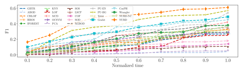
Figure 3: F1 scores at different normalized time checkpoints for online straggler identification on Alibaba traces (higher is better).

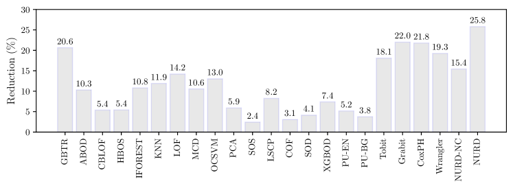
Figure 4: Average reduction in job completion time with unlimited machines on Google traces (higher is better).

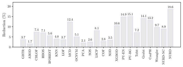
Figure 5: Average reduction in job completion time with unlimited machines on Alibaba traces (higher is better).

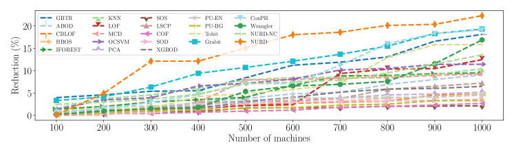
Figure 6: Reduction in job completion time with different numbers of machines on Google traces (higher is better).

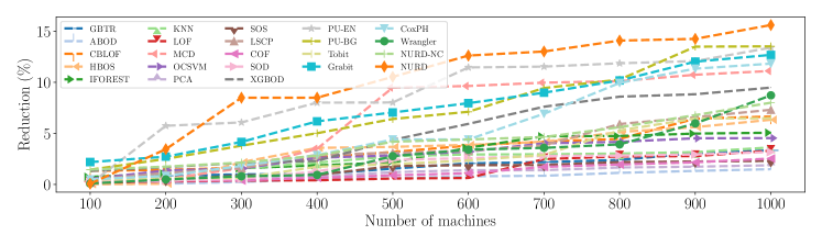
Figure 7: Reduction in job completion time with different numbers of machines on Alibaba traces (higher is better).

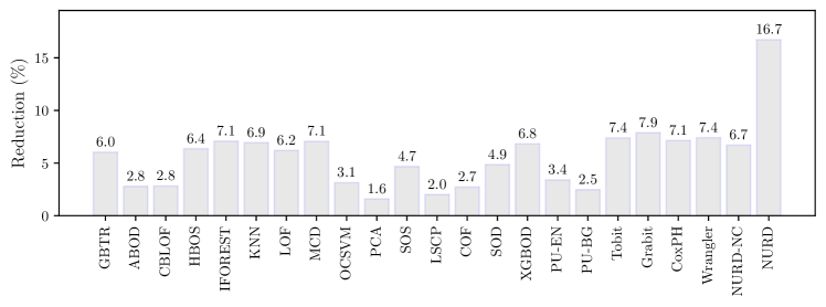
Figure 8: Reduction in job completion time averaged over all number of machines on Google traces (higher is better).

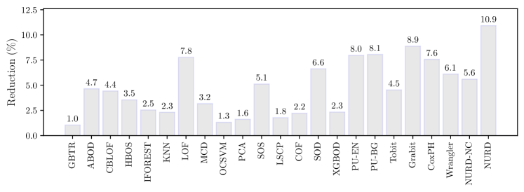
Figure 9: Reduction in job completion time averaged over all number of machines on Alibaba traces (higher is better).

The key takeaways of our evaluation are as follows. Compared to the best baseline approach:

• Nurd achieves 11 and 2 percentage point increases in the F1 score for Google and Alibaba production traces, respectively (Table 3).

• Nurd identifies stragglers earlier (Figure 2 and 3).

• Nurd has 3.8 and 3.5 percentage point improvements in job completion time when more machines are available than tasks (Figure 4 and 5).

• Nurd has 8.8 and 2.0 percentage point improvements in job completion time when fewer machines are available than tasks (Figure 6, 7, 8, and 9).

7.1 How accurate are Nurd’s predictions?

Table 3 shows the average prediction results over all jobs. If a task is predicted to be a non-straggler at the $t$-th time point, it will be evaluated again at $(t+1)$-th time point if it is not finished. If a task is predicted to be a straggler, it will not be evaluated again. We use F1 score as the evaluation metric, and also show true positive rate (TPR), false positive rate (FPR), and false negative rate (FNR) to illustrate the tradeoffs between these metrics.

We can see that the supervised learning method GBTR achieves low TPR and FPR because it is greatly impacted by a lack of stragglers at training: i.e., it predicts most tasks to be non-stragglers. The outlier detection methods have either both high TPR and FPR or both low TPR and FPR, which lead to low F1. It is not surprising since as unsupervised learning methods, the outlier detection methods do not utilize the knowledge of the observed latency. Therefore, it is difficult to assign an explicit separation boundary between stragglers and non-stragglers. As semi-supervised learning methods, PU-EN and PU-BG achieve impressive TPR, but fail to keep FPR consistently low. We notice that they tend to predict all tasks to be stragglers in early time checkpoints. Remember that there is a training and test distribution drift between training and test set for online straggler prediction. As classifiers rather than regressors, PU learners aggressively classify tasks that are different from training tasks (non-stragglers) to be stragglers.

Censored and survival regression methods including Tobit, Grabit, and CoxPH are better than outlier detection and PU methods since they incorporate both features and latency at training. They are worse than Nurd mainly due to the fact that they heavily rely on pre-specified distribution (e.g., Gaussian), while the latency distributions for different jobs are hard to specify in advance (e.g., some are long-tailed). Wrangler achieves both high TPR and FPR, mainly because its offline oversampling makes the prediction biased towards stragglers. Also, its linear classifier is limited in characterizing the nonlinear relationships between features and latency. Regarding our methods, both Nurd-NC and Nurd have high TPRs, but Nurd-NC fails to keep FPR low while Nurd does, which demonstrates the effectiveness of the calibration that accounts for the latency threshold in the weighting function. Overall, Nurd has the best F1 scores: at least 11 and 2 percentage point increases relatively to the other methods for Google and Alibaba traces, respectively.

Furthermore, we note that the best prior approaches are different on Google and Alibaba, while Nurd achieves the best results on both datasets indicating its approach is more generalizable: Grabit’s F1 score is second best (after Nurd on Google, but 10 points worse than Nurd on Alibaba, while PU-BG’s F1 is second best for Alibaba, but 65 points worse on Google. These results demonstrate that Nurd’s reweighting strategy has a dramatic positive effect on online straggler prediction because it makes no assumptions about the underlying data distributions or the existence of labels.

7.2 Does Nurd identify stragglers early?

To illustrate the streaming results when the jobs are running, we compute F1 scores at different time checkpoints. Since different jobs have different total running time, we sample results from 10 time checkpoints for each job and regard them as normalized time. Figure 2 and 3 show the results averaged over all jobs from Google and Alibaba traces, respectively, where the x-axis represents the normalized time between 0 and 1, and y-axis represents the F1 scores. We can see that, for Google traces, Nurd outperforms all other methods at all time points except the very beginning. For Alibaba traces, Nurd outperforms all other methods throughout the run time. These results show that Nurd identifies more stragglers earlier than other methods.

7.3 Does Nurd improve completion time?

We evaluate how Nurd contributes to reducing job completion time by augmenting existing schedulers with improved straggler predictions. The key idea of the schedulers described in section 5 is to relaunch the task on a new machine once the task is predicted to straggle. In our experiments, the new completion time for a rescheduled task is randomly sampled from the existing execution times. We show results in the following two different situations.

More machines than tasks. When more machines are available than tasks for each job, a task that is predicted to straggle is terminated and relaunched on a new machine immediately (Algorithm 2). Figure 4 and 5 show the results for Google and Alibaba traces respectively, with the x-axis represents the method and the y-axis represents the reduction in job completion time (higher is better). We can see that Nurd has the highest reductions, 25.8% and 18.6% for Google and Alibaba traces respectively, which are 3.8 and 3.5 percentage point improvements compared to the best baseline approach. Nurd achieves these improvements due to its early and accurate predictions for stragglers.

Fewer machines than tasks. When fewer machines are available than tasks for each job, the scheduler needs to check if a new machine is available for relaunch if a task is predicted to straggle (Algorithm 3). We study how reduction in completion time will change as a function of the number of machines. Figure 6 and 7 show the results, where the x-axis shows the number of machines from 100 to 900, and the y-axis shows the reduction in job completion time (higher is better). As the number of machines increases, the reductions also increase, and Nurd has the highest reductions compared to all other methods at all numbers except the small size (i.e., 100 and 200). We also compute the reduction averaged over all number of machines in Figure 8 and 9, where x-axis represents different methods, and y-axis represents the average reduction. We can see that Nurd Nurd has the highest reductions, 16.7% and 10.9% for Google and Alibaba traces respectively, which are 8.8 and 2.0 percentage point improvements compared to the best baseline approach. These results demonstrate that Nurd can be easily incorporated with different types of schedulers and effectively reduce the job completion time.

8 Conclusion

This paper introduces Nurd, a novel negative-unlabeled learning approach for online straggler prediction that requires no labeled positive examples or assumptions on latency distributions. The key idea is to train a predictor using finished tasks of non-stragglers to predict latency for unlabeled running tasks, and then reweight each unlabeled task’s prediction based on a weighting function of its feature space. Extensive evaluation results on two real-world production traces demonstrates the effectiveness of Nurd for online straggler prediction. Looking ahead, there is a possibility to apply transfer learning Pan & Yang (2009) to incorporate knowledge from other jobs to improve predictions. We will incorporate transfer learning and deploy our methods in real-world datacenters for future datacenter-scale research.

References

- (1) Alibaba trace. https://github.com/alibaba/clusterdata.
- (2) Google trace. https://github.com/google/cluster-data.
- Adya et al. (2016) Adya, A., Myers, D., Howell, J., Elson, J., Meek, C., Khemani, V., Fulger, S., Gu, P., Bhuvanagiri, L., Hunter, J., Peon, R., Kai, L., Shraer, A., Merchant, A., and Lev-Ari, K. Slicer: Auto-sharding for datacenter applications. In Keeton, K. and Roscoe, T. (eds.), 12th USENIX Symposium on Operating Systems Design and Implementation, OSDI 2016, Savannah, GA, USA, November 2-4, 2016, pp. 739–753. USENIX Association, 2016.
- Aktas & Soljanin (2019) Aktas, M. F. and Soljanin, E. Straggler mitigation at scale. IEEE/ACM Transactions on Networking, 27(6):2266–2279, 2019.
- Aktas et al. (2017) Aktas, M. F., Peng, P., and Soljanin, E. Effective straggler mitigation: Which clones should attack and when? ACM SIGMETRICS Performance Evaluation Review, 45(2):12–14, 2017.
- Alam et al. (2019) Alam, M., Gottschlich, J., Tatbul, N., Turek, J. S., Mattson, T., and Muzahid, A. A zero-positive learning approach for diagnosing software performance regressions. Advances in Neural Information Processing Systems, 32:11627–11639, 2019.
- (7) Alibaba. Alibaba production cluster trace data. https://github.com/alibaba/clusterdata.
- Ananthanarayanan et al. (2010) Ananthanarayanan, G., Kandula, S., Greenberg, A., Stoica, I., Lu, Y., Saha, B., and Harris, E. Reining in the outliers in map-reduce clusters using mantri. In Proceedings of the 9th USENIX Conference on Operating Systems Design and Implementation, OSDI’10, pp. 265–278, USA, 2010.
- Ananthanarayanan et al. (2011) Ananthanarayanan, G., Agarwal, S., Kandula, S., Greenberg, A., Stoica, I., Harlan, D., and Harris, E. Scarlett: Coping with skewed content popularity in mapreduce clusters. In Proceedings of the Sixth Conference on Computer Systems, EuroSys’11, pp. 287–300, New York, NY, USA, 2011. ISBN 9781450306348. doi: 10.1145/1966445.1966472.
- Ananthanarayanan et al. (2013) Ananthanarayanan, G., Ghodsi, A., Shenker, S., and Stoica, I. Effective straggler mitigation: Attack of the clones. In Proceedings of the 10th USENIX Conference on Networked Systems Design and Implementation, NSDI’13, pp. 185–198, USA, 2013.
- Ayers et al. (2019) Ayers, G., Nagendra, N. P., August, D. I., Cho, H. K., Kanev, S., Kozyrakis, C., Krishnamurthy, T., Litz, H., Moseley, T., and Ranganathan, P. Asmdb: understanding and mitigating front-end stalls in warehouse-scale computers. In Proceedings of the 46th International Symposium on Computer Architecture, pp. 462–473, 2019.
- Bekker & Davis (2020) Bekker, J. and Davis, J. Learning from positive and unlabeled data: A survey. Machine Learning, 109(4):719–760, 2020.
- Belay et al. (2014) Belay, A., Prekas, G., Klimovic, A., Grossman, S., Kozyrakis, C., and Bugnion, E. Ix: A protected dataplane operating system for high throughput and low latency. In 11th USENIX Symposium on Operating Systems Design and Implementation (OSDI 14), pp. 49–65, 2014.
- Breunig et al. (2000) Breunig, M. M., Kriegel, H.-P., Ng, R. T., and Sander, J. Lof: identifying density-based local outliers. In Proceedings of the 2000 ACM SIGMOD international conference on Management of data, pp. 93–104, 2000.
- Cepeda et al. (2003) Cepeda, M. S., Boston, R., Farrar, J. T., and Strom, B. L. Comparison of logistic regression versus propensity score when the number of events is low and there are multiple confounders. American journal of epidemiology, 158(3):280–287, 2003.
- Chandola et al. (2007) Chandola, V., Banerjee, A., and Kumar, V. Outlier detection: A survey. ACM Computing Surveys, 14:15, 2007.
- Chandola et al. (2009) Chandola, V., Banerjee, A., and Kumar, V. Anomaly detection: A survey. ACM computing surveys (CSUR), 41(3):1–58, 2009.
- Chen & Guestrin (2016) Chen, T. and Guestrin, C. Xgboost: A scalable tree boosting system. In Proceedings of the 22nd acm sigkdd international conference on knowledge discovery and data mining, pp. 785–794, 2016.
- Cox (1972) Cox, D. R. Regression models and Life-Tables. J. R. Stat. Soc. Series B Stat. Methodol., 34(2):187–220, 1972.
- Dean & Barroso (2013) Dean, J. and Barroso, L. A. The tail at scale. Commun. ACM, 56(2):74–80, February 2013. ISSN 0001–0782.
- Dean & Ghemawat (2004) Dean, J. and Ghemawat, S. Mapreduce: Simplified data processing on large clusters. In Proceedings of the 6th Conference on Symposium on Operating Systems Design and Implementation - Volume 6, OSDI’04, pp. 10, USA, 2004.
- Elkan & Noto (2008) Elkan, C. and Noto, K. Learning classifiers from only positive and unlabeled data. In Proceedings of the 14th ACM SIGKDD international conference on Knowledge discovery and data mining, pp. 213–220, 2008.
- Goldstein & Dengel (2012) Goldstein, M. and Dengel, A. Histogram-based outlier score (hbos): A fast unsupervised anomaly detection algorithm. KI-2012: Poster and Demo Track, pp. 59–63, 2012.
- Guo et al. (2019) Guo, J., Chang, Z., Wang, S., Ding, H., Feng, Y., Mao, L., and Bao, Y. Who limits the resource efficiency of my datacenter: An analysis of alibaba datacenter traces. In Proceedings of the International Symposium on Quality of Service, IWQoS ’19, New York, NY, USA, 2019. Association for Computing Machinery.
- Handley et al. (2017) Handley, M., Raiciu, C., Agache, A., Voinescu, A., Moore, A. W., Antichi, G., and Wójcik, M. Re-architecting datacenter networks and stacks for low latency and high performance. In Proceedings of the Conference of the ACM Special Interest Group on Data Communication, SIGCOMM 2017, Los Angeles, CA, USA, August 21-25, 2017, pp. 29–42. ACM, 2017.
- Hao et al. (2017) Hao, M., Li, H., Tong, M. H., Pakha, C., Suminto, R. O., Stuardo, C. A., Chien, A. A., and Gunawi, H. S. Mittos: Supporting millisecond tail tolerance with fast rejecting slo-aware os interface. In Proceedings of the 26th Symposium on Operating Systems Principles, SOSP’17’, pp. 168–183, New York, NY, USA, 2017. ISBN 9781450350853.
- Hao et al. (2020) Hao, M., Toksoz, L., Li, N., Halim, E. E., Hoffmann, H., and Gunawi, H. S. Linnos: Predictability on unpredictable flash storage with a light neural network. In 14th USENIX Symposium on Operating Systems Design and Implementation (OSDI 20), pp. 173–190, 2020.
- Haque et al. (2015) Haque, M. E., Eom, Y. H., He, Y., Elnikety, S., Bianchini, R., and McKinley, K. S. Few-to-many: Incremental parallelism for reducing tail latency in interactive services. In Özturk, Ö., Ebcioglu, K., and Dwarkadas, S. (eds.), Proceedings of the Twentieth International Conference on Architectural Support for Programming Languages and Operating Systems, ASPLOS’15, Istanbul, Turkey, March 14-18, 2015, pp. 161–175. ACM, 2015.
- Hardin & Rocke (2004) Hardin, J. and Rocke, D. M. Outlier detection in the multiple cluster setting using the minimum covariance determinant estimator. Computational Statistics & Data Analysis, 44(4):625–638, 2004.
- He et al. (2003) He, Z., Xu, X., and Deng, S. Discovering cluster-based local outliers. Pattern Recognition Letters, 24(9-10):1641–1650, 2003.
- Hosmer et al. (2008) Hosmer, Jr, D. W., Lemeshow, S., and May, S. Applied Survival Analysis: Regression Modeling of Time-to-Event Data. John Wiley & Sons, March 2008.
- Janssens et al. (2012) Janssens, J., Huszár, F., Postma, E., and van den Herik, H. Stochastic outlier selection. Tilburg centre for Creative Computing, techreport 2012-001, 2012.
- Kiryo et al. (2017) Kiryo, R., Niu, G., du Plessis, M. C., and Sugiyama, M. Positive-unlabeled learning with non-negative risk estimator. In Advances in Neural Information Processing Systems, volume 30, 2017.
- Kriegel et al. (2008) Kriegel, H.-P., Schubert, M., and Zimek, A. Angle-based outlier detection in high-dimensional data. In Proceedings of the 14th ACM SIGKDD international conference on Knowledge discovery and data mining, pp. 444–452, 2008.
- Kriegel et al. (2009) Kriegel, H.-P., Kröger, P., Schubert, E., and Zimek, A. Outlier detection in axis-parallel subspaces of high dimensional data. In Pacific-asia conference on knowledge discovery and data mining, pp. 831–838. Springer, 2009.
- Lee et al. (2015) Lee, K., Chu, D., Cuervo, E., Kopf, J., Degtyarev, Y., Grizan, S., Wolman, A., and Flinn, J. Outatime: Using speculation to enable low-latency continuous interaction for mobile cloud gaming. In Borriello, G., Pau, G., Gruteser, M., and Hong, J. I. (eds.), Proceedings of the 13th Annual International Conference on Mobile Systems, Applications, and Services, MobiSys 2015, Florence, Italy, May 19-22, 2015, pp. 151–165. ACM, 2015.
- Lee & Liu (2003) Lee, W. S. and Liu, B. Learning with positive and unlabeled examples using weighted logistic regression. In ICML, volume 3, pp. 448–455, 2003.
- Liu et al. (2008) Liu, F. T., Ting, K. M., and Zhou, Z.-H. Isolation forest. In 2008 eighth ieee international conference on data mining, pp. 413–422. IEEE, 2008.
- Mordelet & Vert (2014) Mordelet, F. and Vert, J.-P. A bagging svm to learn from positive and unlabeled examples. Pattern Recognition Letters, 37:201–209, 2014.
- Nelson et al. (2015) Nelson, J., Holt, B., Myers, B., Briggs, P., Ceze, L., Kahan, S., and Oskin, M. Latency-tolerant software distributed shared memory. In 2015 USENIX Annual Technical Conference (USENIX ATC 15), pp. 291–305, 2015.
- Pan & Yang (2009) Pan, S. J. and Yang, Q. A survey on transfer learning. IEEE Transactions on knowledge and data engineering, 22(10):1345–1359, 2009.
- Penney & Chen (2019) Penney, D. D. and Chen, L. A survey of machine learning applied to computer architecture design. arXiv preprint arXiv:1909.12373, 2019.
- Powell (1986) Powell, J. L. Censored regression quantiles. Journal of econometrics, 32(1):143–155, 1986.
- Quiñonero-Candela et al. (2009) Quiñonero-Candela, J., Sugiyama, M., Lawrence, N. D., and Schwaighofer, A. Dataset shift in machine learning. Mit Press, 2009.
- Ramaswamy et al. (2000) Ramaswamy, S., Rastogi, R., and Shim, K. Efficient algorithms for mining outliers from large data sets. In Proceedings of the 2000 ACM SIGMOD international conference on Management of data, pp. 427–438, 2000.
- Reiss et al. (2011) Reiss, C., Wilkes, J., and Hellerstein, J. L. Google cluster-usage traces: format+ schema. Google Inc., White Paper, pp. 1–14, 2011.
- Reiss et al. (2012) Reiss, C., Tumanov, A., Ganger, G. R., Katz, R. H., and Kozuch, M. A. Heterogeneity and dynamicity of clouds at scale: Google trace analysis. In Proceedings of the third ACM symposium on cloud computing, pp. 1–13, 2012.
- Ren et al. (2015) Ren, X., Ananthanarayanan, G., Wierman, A., and Yu, M. Hopper: Decentralized speculation-aware cluster scheduling at scale. In Proceedings of the 2015 ACM Conference on Special Interest Group on Data Communication, SIGCOMM’15, pp. 379–392, New York, NY, USA, 2015. ISBN 9781450335423.
- Rosenbaum & Rubin (1983) Rosenbaum, P. R. and Rubin, D. B. The central role of the propensity score in observational studies for causal effects. Biometrika, 70(1):41–55, 1983.
- Schölkopf et al. (2001) Schölkopf, B., Platt, J. C., Shawe-Taylor, J., Smola, A. J., and Williamson, R. C. Estimating the support of a high-dimensional distribution. Neural computation, 13(7):1443–1471, 2001.
- Schwarzkopf & Bailis (2018) Schwarzkopf, M. and Bailis, P. Research for practice: cluster scheduling for datacenters. Commun. ACM, 61(5):50–53, 2018.
- Shyu et al. (2003) Shyu, M.-L., Chen, S.-C., Sarinnapakorn, K., and Chang, L. A novel anomaly detection scheme based on principal component classifier. Technical report, MIAMI UNIV CORAL GABLES FL DEPT OF ELECTRICAL AND COMPUTER ENGINEERING, 2003.
- Sigrist & Hirnschall (2019) Sigrist, F. and Hirnschall, C. Grabit: Gradient tree-boosted tobit models for default prediction. Journal of Banking & Finance, 102:177–192, 2019.
- Sipple (2020) Sipple, J. Interpretable, multidimensional, multimodal anomaly detection with negative sampling for detection of device failure. In International Conference on Machine Learning, pp. 9016–9025. PMLR, 2020.
- Tang et al. (2002) Tang, J., Chen, Z., Fu, A. W.-C., and Cheung, D. W. Enhancing effectiveness of outlier detections for low density patterns. In Pacific-Asia Conference on Knowledge Discovery and Data Mining, pp. 535–548. Springer, 2002.
- Tian et al. (2005) Tian, L., Zucker, D., and Wei, L. On the cox model with time-varying regression coefficients. Journal of the American statistical Association, 100(469):172–183, 2005.
- Tobin (1958) Tobin, J. Estimation of relationships for limited dependent variables. Econometrica: journal of the Econometric Society, pp. 24–36, 1958.
- Yadwadkar et al. (2014) Yadwadkar, N. J., Ananthanarayanan, G., and Katz, R. Wrangler: Predictable and faster jobs using fewer resources. In Proceedings of the ACM Symposium on Cloud Computing, SOCC’14, pp. 1–14, New York, NY, USA, 2014. ISBN 9781450332521.
- Zaharia et al. (2008) Zaharia, M., Konwinski, A., Joseph, A. D., Katz, R., and Stoica, I. Improving mapreduce performance in heterogeneous environments. In Proceedings of the 8th USENIX Conference on Operating Systems Design and Implementation, OSDI’08, pp. 29–42, USA, 2008.
- Zhang et al. (2013) Zhang, K., Schölkopf, B., Muandet, K., and Wang, Z. Domain adaptation under target and conditional shift. In International Conference on Machine Learning, pp. 819–827. PMLR, 2013.
- Zhao & Hryniewicki (2018) Zhao, Y. and Hryniewicki, M. K. Xgbod: improving supervised outlier detection with unsupervised representation learning. In 2018 International Joint Conference on Neural Networks (IJCNN), pp. 1–8. IEEE, 2018.
- Zhao et al. (2019a) Zhao, Y., Nasrullah, Z., Hryniewicki, M. K., and Li, Z. Lscp: Locally selective combination in parallel outlier ensembles. In Proceedings of the 2019 SIAM International Conference on Data Mining, pp. 585–593. SIAM, 2019a.
- Zhao et al. (2019b) Zhao, Y., Nasrullah, Z., and Li, Z. Pyod: A python toolbox for scalable outlier detection. Journal of Machine Learning Research, 20(96):1–7, 2019b.
- Zheng & Lee (2018) Zheng, P. and Lee, B. C. Hound: Causal learning for datacenter-scale straggler diagnosis. In the 2018 ACM International Conference on Measurement and Modeling of Computer Systems, SIGMETRICS’18, pp. 59–61, New York, NY, USA, 2018. ISBN 9781450358460.
- Zhou et al. (2020) Zhou, Q., Guo, S., Lu, H., Li, L., Guo, M., Sun, Y., and Wang, K. Falcon: Addressing stragglers in heterogeneous parameter server via multiple parallelism. IEEE Transactions on Computers, 70(1):139–155, 2020.
- Zhou et al. (2021) Zhou, Q., Guo, S., Lu, H., Li, L., Guo, M., Sun, Y., and Wang, K. A comprehensive inspection of the straggler problem. Computer, 54(10):4–5, 2021.