Next-to-leading order corrections to decays of the heavier CP-even Higgs boson
in the two Higgs doublet model

Abstract

We investigate the impact of electroweak (EW), scalar and QCD corrections to the full set of decay branching ratios of an additional CP-even Higgs boson ($H$) in the two Higgs doublet model with a softly broken $Z_{2}$ symmetry. We employ the improved gauge independent on-shell scheme in the renormalized vertices. We particularly focus on the scenario near the alignment limit in which couplings of the discovered 125 GeV Higgs boson ($h$) coincide with those of the standard model while the $Hhh$ coupling vanishes at tree level. The renormalized decay rate for $H\to hh$ can significantly be changed from the prediction at tree level due to non-decoupling loop effects of additional Higgs bosons, even in the near alignment case. We find that the radiative corrections to the branching ratio of $H\to hh$ can be a few ten percent level in the case with the masses of additional Higgs bosons being degenerate under the constraints of perturbative unitarity, vacuum stability and the EW precision data. Further sizable corrections can be obtained for the case with a mass difference among the additional Higgs bosons.

I Introduction

Current data at LHC show that properties of the discovered Higgs boson ($h$) ATLAS:2012yve ; CMS:2012qbp are consistent with those of the standard model (SM) Higgs boson within experimental uncertainties ATLAS:2019nkf ; CMS:2020gsy . In addition, there is so far no report which clearly indicates signatures of new particles from collider experiments. On the other hand, new physics beyond the SM must exist, because there are phenomena which cannot be explained in the SM such as neutrino oscillations, dark matter and baryon asymmetry of the Universe. In such new physics models, the Higgs sector is often extended from the minimal one assumed in the SM, and its structure depends on new physics scenarios. Therefore, clarifying the structure of the Higgs sector is important to determine the direction of new physics.

One of the useful ways to determine the structure of extended Higgs sectors is to measure deviations in various observables of $h$ from SM predictions. We can extract information on the structure such as the number of additional Higgs fields and their representations from the pattern of the deviations Kanemura:2014bqa . Furthermore, the mass scale of extra Higgs bosons can be deduced from the size of the deviations Kanemura:2004mg ; Kanemura:2014dja ; Kanemura:2015mxa ; Kanemura:2017wtm ; Kanemura:2018yai ; Kanemura:2019kjg ; Krause:2016oke ; Krause:2016xku ; Krause:2019qwe ; Arhrib:2003vip . Because the precise measurements of cross sections, decay branching ratios (BRs) and the width of the Higgs boson will be performed at future collider experiments such as the high luminosity LHC (HL-LHC) Cepeda:2019klc , International Linear Collider (ILC) Baer:2013cma ; Fujii:2017vwa ; Asai:2017pwp ; LCCPhysicsWorkingGroup:2019fvj , Circular Electron Positron Collider (CEPC) CEPC-SPPCStudyGroup:2015csa and Future Circular Collider (FCC-ee) TLEPDesignStudyWorkingGroup:2013myl , precise predictions of these observables including radiative corrections are necessary to compare these measurements. There are several public tools to calculate radiative corrections in models with an extended Higgs sector; i.e., H-COUP Kanemura:2017gbi ; Kanemura:2019slf , 2HDECAY Krause:2018wmo and Prophecy4f Denner:2019fcr .

Another way is direct searches for additional Higgs bosons. The current situation mentioned above ATLAS:2020zms ; ATLAS:2019tpq ; ATLAS:2018rvc ; ATLAS:2018rnh ; ATLAS:2017uhp ; ATLAS:2020tlo ; ATLAS:2020qiz ; ATLAS:2020gxx ; ATLAS:2021upq ; CMS:2018hir ; CMS:2019pzc ; CMS:2017ucf ; CMS:2017aza ; CMS:2019bnu ; CMS:2019kca ; CMS:2020imj ; CMS:2019bfg would indicate that additional Higgs bosons are too heavy to be directly detected, or otherwise their masses stay at the electroweak (EW) scale but their decay products are hidden by huge backgrounds. The latter possibility suggests that the Higgs sector is nearly aligned without decoupling Gunion:2002zf ; Craig:2013hca ; Carena:2013ooa ; Haber:2015pua ; Bernon:2015qea , in which couplings of the discovered Higgs boson are aligned to those of the SM. In this case, decays of additional Higgs bosons into a lighter Higgs boson, “Higgs to Higgs decays”, are suppressed due to the small mixing with $h$, which can be regarded as a golden channel for the direct searches, see e.g., $H\to hh$ and $A\to Zh$ in Refs. Dumont:2014wha ; Craig:2015jba ; Bernon:2015qea ; Bernon:2015wef ; Chowdhury:2017aav ; Su:2019dsf ; Kling:2020hmi ; Kanemura:2014dea ; Aiko:2020ksl . It has been shown in Ref. Aiko:2020ksl that by considering the synergy between direct searches for additional Higgs bosons at the HL-LHC and precise measurements of the $h$ couplings at the ILC, wide regions of the parameter space on extended Higgs sectors can be explored.

Such a synergy analysis discussed in Ref. Aiko:2020ksl has been performed at leading order (LO) in EW interactions. However, tree level analyses might not be sufficient because of the following reasons. First, they have analyzed the excluded and testable parameter regions inputting the tree level $hVV$ coupling ($V=W,Z$) as constraints from indirect searches. If we take into account loop corrections, the $hVV$ coupling is modified. Second, decay rates of the Higgs to Higgs decay processes can be significantly changed at one-loop level from the prediction at tree level, because some of one-loop diagrams do not vanish at the alignment limit and can be sizable due to the non-decoupling effects of additional Higgs bosons. Therefore, in order to see the synergy in a more realistic way, radiative corrections to both the discovered Higgs boson couplings and the decay BRs of additional Higgs bosons should be taken into account. Radiative corrections to decays of additional Higgs bosons have been studied in Refs. Barger:1991ed ; Osland:1998hv ; Philippov:2006th ; Williams:2007dc ; Williams:2011bu ; Krause:2016xku for a heavy CP-even Higgs boson, in Refs. Krause:2019qwe ; Chankowski:1992es for a CP-odd Higgs boson and in Refs. Akeroyd:1998uw ; Akeroyd:2000xa ; Santos:1996hs ; Krause:2016oke ; Aiko:2021can for singly charged Higgs bosons.

In this paper, we investigate the impact of next-leading-order (NLO) corrections in EW and scalar interactions to the decay BRs of an additional CP-even Higgs boson ($H$) in the two Higgs doublet model (THDM) with a soft broken $Z_{2}$ symmetry Glashow:1976nt ; Paschos:1976ay as a simple but important example. We compute decay rates of $H\to hh$, $H\to f\bar{f}$, $H\to VV$, $H\to\gamma\gamma$, $H\to Z\gamma$ and $H\to gg$ at one-loop level based on the improved on-shell renormalization scheme without gauge dependences, while QCD corrections are also included in decay rates of $H\to q\bar{q}$, $H\to\gamma\gamma$, $H\to Z\gamma$ and $H\to gg$. We study the relation between model parameters; e.g., such as masses of additional Higgs bosons and mixing parameters, and the effects of radiative corrections for the $H\to hh$ decay. Moreover, we clarify how the one-loop corrections can significantly change the tree level predictions in the scenario with nearly alignment, and the correlation between the deviation of the $h\to WW^{*}$ decay from the SM prediction and the one-loop corrected decay rate of $H\to hh$ under theoretical and experimental constraints. We also study the correlation between the BR of the $H\to hh$ decay and the deviation of the one-loop corrected $hhh$ vertex of the THDM  Kanemura:2004mg ; Kanemura:2015mxa ; Kanemura:2017wtm from that of the SM, which is important for testing the EW baryogenesis scenario Kanemura:2002vm ; Kanemura:2004ch ; Grojean:2004xa ; Braathen:2019zoh ; Braathen:2020vwo . Finally, we give results of decay BRs of other decay processes in several scenarios.

This paper is organized as follows. In Sec. II, we define the THDMs and we mention the current situation of experimental constraints. In Sec. III, we define our renormalization scheme, and give renormalized vertices $Hhh$, $Hf\bar{f}$ ($f=t,~{}b,~{}\tau,~{}c$) and $HVV$ ($V=W,~{}Z$). In Sec. IV, we give formulae of one-loop corrected decay rates of $H\to hh$, $H\to f\bar{f}$ and $H\to VV$. Numerical evaluations of these decay rates are shown in Sec. V. Discussions and conclusions are respectively given in Sec. VI and VII. In Appendix, we present explicit analytic formulae of 1PI diagrams for the $Hhh$ vertex.

II Model

The Higgs sector is composed of two isospin doublet fields $\Phi_{1}$ and $\Phi_{2}$ with hypercharge $Y=1/2$. In order to avoid flavor changing neutral currents mediated by Higgs bosons at tree level, we impose a discrete $Z_{2}$ symmetry to the model, where $\Phi_{1}$ and $\Phi_{2}$ are transformed to $+\Phi_{1}$ and $-\Phi_{2}$ Glashow:1976nt ; Paschos:1976ay , respectively.

The Higgs potential is given under the $Z_{2}$ symmetry by

$$V =m_{1}^{2}|\Phi_{1}|^{2}+m_{2}^{2}|\Phi_{2}|^{2}-m_{3}^{2}(\Phi_{1}^{\dagger}\Phi_{2}+\textrm{h.c.})$$

$$+\frac{\lambda_{1}}{2}|\Phi_{1}|^{4}+\frac{\lambda_{2}}{2}|\Phi_{2}|^{4}+\lambda_{3}|\Phi_{1}|^{2}|\Phi_{2}|^{2}+\lambda_{4}|\Phi_{1}^{\dagger}\Phi_{2}|^{2}+\frac{\lambda_{5}}{2}\left[(\Phi_{1}^{\dagger}\Phi_{2})^{2}+\textrm{h.c.}\right],$$ (1)

where the $m_{3}^{2}$ term softly breaks the $Z_{2}$ symmetry. In general, $m_{3}^{2}$ and $\lambda_{5}$ are complex, but we assume these parameters to be real. The Higgs fields are parameterized as

$$\Phi_{i}=\begin{pmatrix}w_{i}^{+}\\ \frac{1}{\sqrt{2}}(h_{i}+v_{i}+iz_{i})\end{pmatrix},\,\,\,\left(i=1,2\right),$$ (2)

where $v_{1}$ and $v_{2}$ are the vacuum expectation values (VEVs) with $v=\sqrt{v_{1}^{2}+v_{2}^{2}}\simeq 246$ GeV, and their ratio is parameterized as $\tan\beta=v_{2}/v_{1}$. The mass eigenstates of the Higgs bosons are defined as follows,

$$\begin{pmatrix}w_{1}^{\pm}\\ w_{2}^{\pm}\end{pmatrix}=R(\beta)\begin{pmatrix}G^{\pm}\\ H^{\pm}\end{pmatrix},\,\,\,\begin{pmatrix}z_{1}\\ z_{2}\end{pmatrix}=R(\beta)\begin{pmatrix}G^{0}\\ A\end{pmatrix},\,\,\,\begin{pmatrix}h_{1}\\ h_{2}\end{pmatrix}=R(\alpha)\begin{pmatrix}H\\ h\end{pmatrix},$$ (3)

where

$$R(\theta)=\begin{pmatrix}c_{\theta}&-s_{\theta}\\ s_{\theta}&c_{\theta}\end{pmatrix},$$ (4)

with $s_{\theta}\equiv\sin\theta$ and $c_{\theta}\equiv\cos\theta$. In Eq. (3), $H^{\pm}$, $A$, $H$ and $h$ are the physical mass eigenstates, while $G^{\pm}$ and $G^{0}$ are the Nambu-Goldstone bosons. After imposing the tadpole conditions, the masses of the charged and CP-odd Higgs bosons are expressed as

$$m_{H^{\pm}}^{2}=M^{2}-\frac{v^{2}}{2}(\lambda_{4}+\lambda_{5}),\,\,\,m_{A}^{2}=M^{2}-v^{2}\lambda_{5},$$ (5)

where $M^{2}$ is defined as $M^{2}=m_{3}^{2}/(s_{\beta}c_{\beta})$. The masses of the CP-even Higgs bosons and the mixing angle $\beta-\alpha$ are given by

$$m_{H}^{2}=M_{11}^{2}c_{\beta-\alpha}^{2}+M_{22}^{2}s_{\beta-\alpha}^{2}-M_{12}^{2}s_{2(\beta-\alpha)},$$ (6)

$$m_{h}^{2}=M_{11}^{2}s_{\beta-\alpha}^{2}+M_{22}^{2}c_{\beta-\alpha}^{2}+M_{12}^{2}s_{2(\beta-\alpha)},$$ (7)

$$\tan 2(\beta-\alpha)=-\frac{2M_{12}^{2}}{M_{11}^{2}-M_{22}^{2}},$$ (8)

where

$$M_{11}^{2} =v^{2}\left[\lambda_{1}c_{\beta}^{4}+\lambda_{2}s_{\beta}^{4}+2(\lambda_{3}+\lambda_{4}+\lambda_{5})s_{\beta}^{2}c_{\beta}^{2}\right],$$ (9)

$$M_{22}^{2} =M^{2}+\frac{v^{2}}{4}s_{2\beta}^{2}\left[\lambda_{1}+\lambda_{2}-2(\lambda_{3}+\lambda_{4}+\lambda_{5})\right],$$ (10)

$$M_{12}^{2} =\frac{v^{2}}{2}s_{2\beta}\left[-\lambda_{1}c_{\beta}^{2}+\lambda_{2}s_{\beta}^{2}+(\lambda_{3}+\lambda_{4}+\lambda_{5})c_{2\beta}\right],$$ (11)

with $M_{ij}^{2}$ being elements of the mass matrix in the basis of $R(\beta)(h_{1},h_{2})^{T}$. In the following, we identify $h$ as the discovered Higgs boson with a mass of 125 GeV. The 8 parameters in Eq. (1) can be expressed by the following 8 parameters,

$$m_{h}^{2},~{}m_{H}^{2},~{}m_{A}^{2},~{}m_{H^{\pm}}^{2},~{}M^{2},~{}s_{\beta-\alpha},~{}\tan\beta,~{}v,$$ (12)

where we define $\tan\beta>0$ and $0\leq s_{\beta-\alpha}\leq 1$, while $c_{\beta-\alpha}$ can be either positive and negative. These parameters can be constrained by considering bounds from perturbative unitarity Kanemura:2015ska ; Kanemura:1993hm ; Akeroyd:2000wc ; Ginzburg:2005dt and vacuum stability Deshpande:1977rw ; Klimenko:1984qx ; Sher:1988mj ; Nie:1998yn . Throughout the paper, we take $M^{2}\geq 0$ by which the true vacuum condition is satisfied Barroso:2013awa .

For the later discussion, we here give expressions of the triple scalar couplings as

$$\lambda_{hhh} =-\frac{m_{h}^{2}}{2v}s_{\beta-\alpha}+\frac{M^{2}-m_{h}^{2}}{v}c_{\beta-\alpha}^{2}\left[s_{\beta-\alpha}+\frac{c_{\beta-\alpha}}{2}(\cot\beta-\tan\beta)\right],$$ (13)

$$\lambda_{Hhh} =-\frac{c_{\beta-\alpha}}{2vs_{2\beta}}\left[(2m_{h}^{2}+m_{H}^{2}-3M^{2})s_{2\alpha}+M^{2}s_{2\beta}\right],$$ (14)

$$\lambda_{HHh} =\frac{s_{\beta-\alpha}}{2v}[(2M^{2}-2m_{H}^{2}-m_{h}^{2})s_{\beta-\alpha}^{2}+2(3M^{2}-2m_{H}^{2}-m_{h}^{2})\cot 2\beta s_{\beta-\alpha}c_{\beta-\alpha}$$

$$-(4M^{2}-2m_{H}^{2}-m_{h}^{2})c_{\beta-\alpha}^{2}],$$ (15)

where they are defined as $\mathcal{L}=\lambda_{\phi\phi^{\prime}\phi^{\prime\prime}}\phi\phi^{\prime}\phi^{\prime\prime}+\cdots$.

The kinetic term of the Higgs fields is

$$\mathcal{L}_{\mathrm{kin}}=|D_{\mu}\Phi_{1}|^{2}+|D_{\mu}\Phi_{2}|^{2},$$ (16)

where $D_{\mu}$ is the covariant derivative given by $D_{\mu}=\partial_{\mu}-i\frac{g}{2}\tau^{a}W_{\mu}^{a}-i\frac{g^{\prime}}{2}B_{\mu}$. The gauge-gauge-scalar interaction terms in the mass eigenstates are extracted as

$$\mathcal{L}_{\mathrm{kin}} \supset{g}m_{W}g^{\mu\nu}\left(\kappa_{W}^{h}W^{+}_{\mu}W^{-}_{\nu}h+\kappa_{W}^{H}W^{+}_{\mu}W^{-}_{\nu}H\right)+\frac{g_{Z}m_{Z}}{2}g^{\mu\nu}\left(\kappa_{Z}^{h}Z_{\mu}Z_{\nu}h+\kappa_{Z}^{H}Z_{\mu}Z_{\nu}H\right),$$ (17)

where $g_{Z}$ is defined as $g_{Z}\equiv g/\cos\theta_{W}$, and $\kappa_{V}^{\phi}$ ($\phi=h,H$) is the scaling factor obtained as

$$\kappa_{V}^{h}=s_{\beta-\alpha},\,\,\,\kappa_{V}^{H}=c_{\beta-\alpha}.$$ (18)

	$\Phi_{1}$	$\Phi_{2}$	$Q_{L}$	$L_{L}$	$u_{R}$	$d_{R}$	$e_{R}$	$\zeta_{u}$	$\zeta_{d}$	$\zeta_{e}$
Type-I	$+$	$-$	$+$	$+$	$-$	$-$	$-$	$\cot\beta$	$\cot\beta$	$\cot\beta$
Type-II	$+$	$-$	$+$	$+$	$-$	$+$	$+$	$\cot\beta$	$-\tan\beta$	$-\tan\beta$
Type-X	$+$	$-$	$+$	$+$	$-$	$-$	$+$	$\cot\beta$	$\cot\beta$	$-\tan\beta$
Type-Y	$+$	$-$	$+$	$+$	$-$	$+$	$-$	$\cot\beta$	$-\tan\beta$	$\cot\beta$

Table 1: Charge assignment of the $Z_{2}$ symmetry and mixing factors $\zeta_{f}$ ($f=u,d,e$) in each type of the Yukawa interaction.

The most general Yukawa interaction is given under the $Z_{2}$ symmetry as

$$\mathcal{L}_{Y}=-Y_{u}\bar{Q}_{L}(i\tau_{2}\Phi_{i}^{*})u_{R}-Y_{d}\bar{Q}_{L}\Phi_{j}d_{R}-Y_{e}\bar{L}_{L}\Phi_{k}e_{R}+\rm{h.c.},$$ (19)

where $\Phi_{i}$, $\Phi_{j}$ and $\Phi_{k}$ are either $\Phi_{1}$ or $\Phi_{2}$. These labels of the Higgs doublet fields are determined by fixing the $Z_{2}$ charge of each field as summarized in Tab. 1 Barger:1989fj ; Aoki:2009ha . The Yukawa interaction terms are given in terms of the mass eigenstates of the Higgs bosons as

$$\mathcal{L}_{Y} \supset-\sum_{f=u,d,e}\frac{m_{f}}{v}\left(\kappa_{f}^{h}\bar{f}fh+\kappa_{f}^{H}\bar{f}fH+\kappa_{f}^{A}\bar{f}\gamma_{5}fA\right)$$

$$-\frac{\sqrt{2}}{v}\left[\bar{u}V_{ud}(m_{d}\zeta_{d}P_{R}-m_{u}\zeta_{u}P_{L})dH^{+}+m_{e}\zeta_{e}\bar{\nu}P_{R}eH^{+}+\rm{h.c.}\right],$$ (20)

where $I_{f}=1/2$ $(-1/2)$ for $f=u$ $(d,e)$, and $V_{ud}$ is the Cabibbo-Kobayashi-Maskawa matrix element. Scaling factors in Eq. (20) are expressed as,

$$\kappa_{f}^{h}=s_{\beta-\alpha}+\zeta_{f}c_{\beta-\alpha},\quad\kappa_{f}^{H}=c_{\beta-\alpha}-\zeta_{f}s_{\beta-\alpha},\quad\kappa_{f}^{A}=-2iI_{f}\zeta_{f},$$ (21)

where $\zeta_{f}$ are given in Tab. 1.

In the limit of $s_{\beta-\alpha}\to 1$, all couplings of $h$ become the same as those of the SM at tree level. We call this limit as the alignment limit. As mentioned in Sec. I, we are interested in the nearly alignment case, so that we introduce a parameter $x$ defined by

$$x\equiv-(\beta-\alpha)+\frac{\pi}{2},$$ (22)

where the limit $x\to 0$ corresponds to the alignment limit. In the nearly alignment case; i.e., $x\simeq 0$, the scaling factors and the triple scalar couplings can be expressed as

$$\kappa_{V}^{h} =1-\frac{x^{2}}{2}+\mathcal{O}(x^{3}),\quad\kappa_{V}^{H}=x+\mathcal{O}(x^{3}),$$ (23)

$$\kappa_{f}^{h} =1+\zeta_{f}x+\frac{x^{2}}{2}+\mathcal{O}(x^{3}),\quad\kappa_{f}^{H}=-\zeta_{f}+x+\frac{x^{2}}{2}\zeta_{f}+\mathcal{O}(x^{3}),$$ (24)

$$\lambda_{ijk} =\lambda_{ijk,0}+\lambda_{ijk,1}x+\lambda_{ijk,2}x^{2}+\mathcal{O}(x^{3}),$$ (25)

with

$$\lambda_{hhh,0}=-\frac{m_{h}^{2}}{2v},\quad\lambda_{hhh,1}=0,\quad\lambda_{hhh,2}=\frac{4M^{2}-3m_{h}^{2}}{4v},$$ (26)

$$\lambda_{Hhh,0}=0,\quad\lambda_{Hhh,1}=\frac{2m_{h}^{2}+m_{H}^{2}-4M^{2}}{2v},\quad\lambda_{Hhh,2}=\frac{(2m_{h}^{2}+m_{H}^{2}-3M^{2})\cot 2\beta}{v},$$ (27)

$$\lambda_{HHh,0}=-\frac{m_{h}^{2}+2m_{H}^{2}-2M^{2}}{2v},\quad\lambda_{HHh,1}=-\frac{(m_{h}^{2}+2m_{H}^{2}-3M^{2})\cot 2\beta}{v},$$

$$\lambda_{HHh,2}=\frac{5m_{h}^{2}+10m_{H}^{2}-14M^{2}}{4v}.$$ (28)

We mention constraints from current experimental data on the THDM.

• Electroweak precision data
  New physics effects on the EW oblique parameters are expressed by the $S$, $T$ and $U$ parameters Peskin:1990zt ; Peskin:1991sw . It has been known that the $T$ parameter represents the violation of the custodial $SU(2)_{V}$ symmetry Haber:1992py ; Pomarol:1993mu ; Herquet:2008eaa ; Kanemura:2011sj . One of the ways to restore the $SU(2)_{V}$ symmetry in the potential is to take $m_{H^{\pm}}=m_{A}$, by which quadratic-power like dependences of Higgs boson masses on the $T$ parameter disappear. 

  By using the global fit of EW parameters Baak:2012kk , new physics effects on the $S$ and $T$ parameters under $U=0$ are constrained by

  $$S=0.05\pm 0.09,\quad T=0.08\pm 0.07,$$ (29)

  with the correlation factor of $+0.91$ Baak:2012kk .

• Signal strength of the Higgs boson $h$
  Measurements of the signal strengths of $h$ constrain mixing parameters $\alpha$ and $\beta$ as seen in Eqs. (18) and (21). According to Refs. CMS:2020gsy ; ATLAS:2021vrm , the parameter regions with $-0.25\lesssim c_{\beta-\alpha}\lesssim 0.01$ for $\tan\beta\simeq 2$ are allowed in the Type-I THDM. In the Type-II, X and Y THDMs, the constraint is given by; e.g., $|c_{\beta-\alpha}|\lesssim 0.1$ for $\tan\beta\simeq 2$, and stronger bounds are taken for larger $\tan\beta$.

• Direct searches for the additional Higgs bosons at LHC
  So far, there has been no report for the discovery of the additional Higgs bosons at LHC, so that lower limits on their masses have been taken. In the THDMs, constraints from the direct searches have been studied by using LHC Run-II data in; e.g., Refs. Aiko:2020ksl ; Kling:2020hmi ; Cheung:2022ndq . In the nearly alignment region, the search for the $pp\to A\to Zh$ process typically excludes the largest region of the parameter space in the four types of THDMs. For instance, $m_{A}\lesssim 2m_{t}$ (900 GeV) are excluded in the case with $s_{\beta-\alpha}=0.99$ and $\tan\beta\simeq 5$ (2)Aiko:2020ksl . For larger values of $1-s_{\beta-\alpha}$, the constraint by this mode becomes stronger. In Type-II and Type-Y, the search for the $pp\to b\bar{b}A\to b\bar{b}Zh$ process also provides severe constraints on the parameter space particularly for the case with larger $\tan\beta$ values. For instance, in the case with $s_{\beta-\alpha}=0.99$ and $\tan\beta=10$, $m_{A}\lesssim 500$ GeV have been excluded Aiko:2020ksl . In addition to the $A\to Zh$ mode, the $H\to hh$ mode can also exclude wide regions of the parameter space. This, however, strongly depends on the value of $M^{2}$, and can be changed by the radiative corrections which will be discussed later.

• Flavor experiments
  The mass of the charged Higgs bosons is restricted by the $B\to X_{s}\gamma$ decay. In Type-II and Type-Y, $m_{H^{\pm}}\lesssim 800$ GeV is excluded for $\tan\beta>2$ Misiak:2017bgg ; Misiak:2020vlo . On the other hand, in Type-I and Type-X, $m_{H^{\pm}}\lesssim 400$ GeV is excluded for $\tan\beta=1$ Misiak:2017bgg ; Misiak:2020vlo . Moreover, in the Type-II case, data of the $B_{s}\to\mu\mu$ decay exclude regions with large $\tan\beta$ Cheng:2015yfu ; Haller:2018nnx ; Enomoto:2015wbn ; e.g., $\tan\beta\gtrsim 25$ for $m_{H^{\pm}}=1$ TeV.

III Renormalized vertices

In this section, we discuss the renormalized vertices for $H$ based on the improved on-shell scheme Kanemura:2017wtm , where gauge dependences in counter terms of mixing angles are removed by adding pinch terms. This treatment is not applied to wave function renormalizations but counter terms from shifts of parameters in the Lagrangian.

In the following discussion, we decompose each renormalized form factor $\hat{\Gamma}_{HXX}$ ($X=h,W,Z,t,b,\tau,c$) as

$$\hat{\Gamma}_{HXX} =\Gamma_{HXX}^{\textrm{Tree}}+\Gamma_{HXX}^{\textrm{1-loop}},$$ (30)

where

$$\Gamma_{HXX}^{\textrm{1-loop}}=\delta\Gamma_{HXX}+\Gamma_{HXX}^{\textrm{1PI}}+\Gamma_{HXX}^{\textrm{Tad}},$$ (31)

with $\Gamma_{HXX}^{\textrm{Tree}}$, $\delta\Gamma_{HXX}$, $\Gamma_{HXX}^{\textrm{1PI}}$ and $\Gamma_{HXX}^{\textrm{Tad}}$ being contributions from tree level diagrams, counter terms, 1PI diagrams and tadpole diagrams inserted to tree level vertices, respectively.

III.1 Renormalization conditions

We discuss renormalization conditions in order to determine the counter terms for the renormalized $HXX$ vertices. The renormalized two-point functions for neutral scalar bosons are expressed as

$$\hat{\Pi}_{ii}[p^{2}]=(p^{2}-m_{i}^{2})(1+\delta Z_{i})-\delta m_{i}^{2}+\tilde{\Pi}_{ii}^{\mathrm{1PI}}[p^{2}],\quad(i=h,H,A)$$ (32)

$$\hat{\Pi}_{hH}[p^{2}]=p^{2}(\delta C_{hH}+\delta C_{Hh})+m_{h}^{2}(\delta\alpha_{f}-\delta C_{hH})-m_{H}^{2}(\delta\alpha_{f}+\delta C_{Hh})+\tilde{\Pi}_{hH}^{\mathrm{1PI}}[p^{2}],$$ (33)

$$\hat{\Pi}_{AG^{0}}[p^{2}]=p^{2}(\delta C_{AG^{0}}+\delta C_{G^{0}A})+m_{A}^{2}(\delta\beta_{f}-\delta C_{AG^{0}})+\tilde{\Pi}_{AG^{0}}^{\mathrm{1PI}}[p^{2}],$$ (34)

where $\delta Z_{i}$, $\delta C_{ij}$, $\delta\alpha_{f}$ and $\delta\beta_{f}$ come from the field shifts defined as

$$\begin{pmatrix}H\\ h\\ \end{pmatrix}\to\begin{pmatrix}1+\frac{1}{2}\delta Z_{H}&\delta C_{Hh}+\delta\alpha_{f}\\ \delta C_{hH}-\delta\alpha_{f}&1+\frac{1}{2}\delta Z_{h}\\ \end{pmatrix}\begin{pmatrix}H\\ h\\ \end{pmatrix},$$ (35)

$$\begin{pmatrix}G^{0}\\ A\\ \end{pmatrix}\to\begin{pmatrix}1+\frac{1}{2}\delta Z_{G^{0}}&\delta C_{G^{0}A}+\delta\beta_{f}\\ \delta C_{AG^{0}}-\delta\beta_{f}&1+\frac{1}{2}\delta Z_{A}\\ \end{pmatrix}\begin{pmatrix}G^{0}\\ A\\ \end{pmatrix}.$$ (36)

We here distinguish $\delta\alpha_{f}$ ($\delta\beta_{f}$) from $\delta\alpha$ ($\delta\beta$) which appears from the parameter shift; i.e., $\alpha\to\alpha+\delta\alpha$ ($\beta\to\beta+\delta\beta$). In Eqs. (32)-(34), $\tilde{\Pi}_{ij}^{\textrm{1PI}}$ is defined as

$$\tilde{\Pi}_{ij}^{\textrm{1PI}}[p^{2}]=\Pi_{ij}^{\textrm{1PI}}[p^{2}]+\Pi_{ij}^{\textrm{Tad}}.$$ (37)

By imposing the following on-shell conditions for the above renormalized two-point functions;

$$\hat{\Pi}_{ii}[m_{i}^{2}]=0,\quad\frac{d}{dp^{2}}\hat{\Pi}_{ii}[p^{2}]\big{|}_{p^{2}=m_{i}^{2}}=1,\,\,\,(i=h,H,A),\quad$$ (38)

the counter terms $\delta m_{i}^{2}$ and $\delta Z_{i}$ are determined as

$$\delta m_{i}^{2}=\tilde{\Pi}_{ii}^{\textrm{1PI}}[m_{i}^{2}],\quad\delta Z_{i}=-\frac{d}{dp^{2}}\Pi_{ii}^{\textrm{1PI}}[p^{2}]\big{|}_{p^{2}=m_{i}^{2}}.$$ (39)

By imposing the on-shell conditions for the mixing two-point functions as

$$\hat{\Pi}_{hH}[m_{h}^{2}]=\hat{\Pi}_{hH}[m_{H}^{2}]=0,\quad\hat{\Pi}_{AG^{0}}[m_{A}^{2}]=\hat{\Pi}_{AG^{0}}[0]=0,$$ (40)

we obtain

$$\delta C_{h}=\frac{1}{2(m_{H}^{2}-m_{h}^{2})}\left(\Pi_{Hh}^{\textrm{1PI}}[m_{h}^{2}]-\Pi_{Hh}^{\textrm{1PI}}[m_{H}^{2}]\right),$$ (41)

$$\delta C_{A}=-\frac{1}{2m_{A}^{2}}\left(\Pi_{Hh}^{\textrm{1PI}}[m_{A}^{2}]-\Pi_{Hh}^{\textrm{1PI}}[0]\right),$$ (42)

$$\delta\alpha_{f}=\frac{1}{2(m_{H}^{2}-m_{h}^{2})}\left(\tilde{\Pi}_{Hh}^{\textrm{1PI}}[m_{h}^{2}]+\tilde{\Pi}_{Hh}^{\textrm{1PI}}[m_{H}^{2}]\right),$$ (43)

$$\delta\beta_{f}=-\frac{1}{2m_{A}^{2}}\left(\tilde{\Pi}_{AG}^{\textrm{1PI}}[m_{A}^{2}]+\tilde{\Pi}_{AG}^{\textrm{1PI}}[0]\right),$$ (44)

where we take $\delta C_{hH}=\delta C_{Hh}\equiv\delta C_{h}$ and $\delta C_{AG^{0}}=\delta C_{G^{0}A}\equiv\delta C_{A}$.

As mentioned above, the counter terms $\delta\alpha$ and $\delta\beta$ should include the pinch term;

$$\delta\alpha=\frac{1}{2(m_{H}^{2}-m_{h}^{2})}\left(\tilde{\Pi}_{Hh}^{\textrm{1PI}}[m_{h}^{2}]+\Pi_{Hh}^{\textrm{PT}}[m_{h}^{2}]+\tilde{\Pi}_{Hh}^{\textrm{1PI}}[m_{H}^{2}]+\Pi_{Hh}^{\textrm{PT}}(m_{H}^{2})\right),$$ (45)

$$\delta\beta=-\frac{1}{2m_{A}^{2}}\left(\tilde{\Pi}_{AG}^{\textrm{1PI}}[m_{A}^{2}]+\Pi_{AG}^{\textrm{PT}}[m_{A}^{2}]+\tilde{\Pi}_{AG}^{\textrm{1PI}}[0]+\Pi_{AG}^{\textrm{PT}}[0]\right),$$ (46)

where explicit formulae of $\Pi_{Hh}^{\textrm{PT}}(p^{2})$ and $\Pi_{AG}^{\textrm{PT}}(p^{2})$ are given in Ref. Kanemura:2017wtm .

The counter term $\delta M^{2}$ cannot be determined by using the on-shell conditions discussed above. Thus, we apply the $\overline{\textrm{MS}}$ scheme to the renormalization of the $hhh$ vertex, and then $\delta M^{2}$ is determined as

$$\delta M^{2}=\frac{M^{2}}{16\pi^{2}v^{2}}\left[2\sum_{f}N_{c}^{f}m_{f}^{2}\kappa_{f}^{2}+4M^{2}-2m_{H^{\pm}}^{2}-m_{A}^{2}+\frac{s_{2\alpha}}{s_{2\beta}}(m_{H}^{2}-m_{h}^{2})-3(2m_{W}^{2}+m_{Z}^{2})\right]\Delta_{\textrm{Div}}$$

$$+\frac{2c_{2\beta}}{s_{2\beta}}\frac{M^{2}}{v}\left(\frac{c_{\beta-\alpha}}{m_{h}^{2}}\textrm{Div(}T_{h}^{\textrm{1PI}})-\frac{s_{\beta-\alpha}}{m_{H}^{2}}\textrm{Div}(T_{H}^{\textrm{1PI}})\right),$$ (47)

where $\Delta_{\textrm{Div}}=1/\epsilon-\gamma_{E}+\log 4\pi$ with $\gamma_{E}$ being the Euler’s constant. In the second line, Div$(T_{h(H)}^{\textrm{1PI}})$ indicates the divergent part of tadpole type diagrams whose explicit formulae are given in Ref. Kanemura:2015mxa . In this prescription, renormalized quantities including $\delta M^{2}$ such as the decay rate of $H\to hh$ have a dependence on the renormalization scale $\mu$.

Finally, the counter terms of the EW parameters $\delta v$, $\delta m_{V}^{2}$, $\delta Z_{V}$, $\delta m_{f}$ and $\delta Z_{V}^{f}$ are given in Ref. Kanemura:2015mxa .

III.2 Renormalized $Hhh$ vertex

The contributions from the tree level diagram and from counter terms are given by

$$\Gamma_{Hhh}^{\textrm{Tree}}=2\lambda_{Hhh},$$ (48)

$$\delta\Gamma_{Hhh}=2\delta\lambda_{Hhh}+\lambda_{Hhh}(\delta Z_{H}+2\delta Z_{h})+6\lambda_{hhh}(\delta C_{h}-\delta\alpha_{f})+4\lambda_{HHh}(\delta C_{h}+\delta\alpha_{f}),$$ (49)

where $\lambda_{hhh}$, $\lambda_{Hhh}$ and $\lambda_{HHh}$ are given in Eqs. (13)-(15), and $\delta\lambda_{Hhh}$ is given by

$$\delta\lambda_{Hhh} =-\lambda_{Hhh}\frac{\delta v}{v}-\frac{s_{2\alpha}c_{\beta-\alpha}}{2vs_{2\beta}}(2\delta m_{h}^{2}+\delta m_{H}^{2})+G_{\alpha}\delta\alpha+G_{\beta}\delta\beta+\frac{3c_{\beta-\alpha}}{2v}\left(\frac{s_{2\alpha}}{s_{2\beta}}-\frac{1}{3}\right)\delta M^{2},$$ (50)

with $G_{\alpha}$ and $G_{\beta}$ being

$$G_{\alpha} =\tan(\beta-\alpha)\lambda_{Hhh}-\frac{c_{2\alpha}c_{\beta-\alpha}}{vs_{2\beta}}(2m_{h}^{2}+m_{H}^{2}-3M^{2}),$$ (51)

$$G_{\beta} =-\frac{c_{\alpha-3\beta}+3c_{\alpha+\beta}}{2s_{2\beta}c_{\beta-\alpha}}\lambda_{Hhh}-\frac{c_{\beta-\alpha}}{v}\cot 2\beta M^{2}.$$ (52)

Explicit formulae of contributions of 1PI diagrams $\Gamma_{Hhh}^{\textrm{1PI}}$ are given in Appendix. As mentioned in the previous subsection, the $Hhh$ coupling depends on the renormalization scale $\mu$.

III.3 Renormalized $Hf\bar{f}$ vertex

The renormalized $Hf\bar{f}$ ($f=t,~{}b,~{}c,~{}\tau$) vertex is expressed in terms of the following form factors,

$$\hat{\Gamma}_{Hff}[p_{1}^{2},p_{2}^{2},q^{2}] =\hat{\Gamma}_{Hff}^{S}+\gamma_{5}\hat{\Gamma}_{Hff}^{P}+\sum_{i=1,2}\left({\ooalign{\hfil/\hfil\crcr$p$}}_{i}\hat{\Gamma}_{Hff}^{V_{i}}+{\ooalign{\hfil/\hfil\crcr$p$}}_{i}\gamma_{5}\hat{\Gamma}_{Hff}^{A_{i}}\right)+{\ooalign{\hfil/\hfil\crcr$p$}}_{1}{\ooalign{\hfil/\hfil\crcr$p$}}_{2}\hat{\Gamma}_{Hff}^{T}+{\ooalign{\hfil/\hfil\crcr$p$}}_{1}{\ooalign{\hfil/\hfil\crcr$p$}}_{2}\gamma_{5}\hat{\Gamma}_{Hff}^{PT},$$ (65)

where $p_{1}^{\mu}$ and $p_{2}^{\mu}$ are the incoming momenta of external particles $f$ and $\bar{f}$, respectively, and $q^{\mu}(=p_{1}^{\mu}+p_{2}^{\mu})$ is the outgoing momentum of $H$. For the case with on-shell fermions; i.e., $p_{1}^{2}=p_{2}^{2}=m_{f}^{2}$, the following relations hold:

$$\hat{\Gamma}_{Hff}^{P}=\hat{\Gamma}_{Hff}^{PT}=0,\hskip 14.22636pt\hat{\Gamma}_{Hff}^{V_{1}}=-\hat{\Gamma}_{Hff}^{V_{2}},\hskip 14.22636pt\hat{\Gamma}_{Hff}^{A_{1}}=-\hat{\Gamma}_{Hff}^{A_{2}}.$$ (66)

The contributions from the tree level diagram and from counter terms are given by

$$\Gamma_{Hff}^{\textrm{Tree},S}=-\frac{m_{f}}{v}\kappa^{H}_{f},\quad\Gamma_{Hff}^{\textrm{Tree},i}=0,$$ (67)

$$\delta\Gamma_{Hff}^{S}=-\frac{m_{f}}{v}\kappa^{H}_{f}\left[\frac{\delta m_{f}}{m_{f}}-\frac{\delta v}{v}+\frac{1}{2}\delta Z_{H}+\delta Z_{V}^{f}+\frac{\delta\kappa^{H}_{f}}{\kappa^{H}_{f}}+\frac{\kappa^{h}_{f}}{\kappa^{H}_{f}}(\delta C_{h}-\delta\alpha_{f})\right],\quad\delta\Gamma_{Hff}^{i}=0,$$ (68)

where the index $i$ runs over $i=\{P,\,V_{1},\,V_{2},\,A_{1},\,A_{2},\,T,\,PT\}$, and

$$\delta\kappa^{H}_{f}=\kappa_{f}^{h}\delta\alpha-\kappa_{f}^{H}\zeta_{f}\delta\beta.$$ (69)

The mixing factor $\zeta_{f}$ and $\kappa_{f}^{\phi}$ ($\phi=h$, $H$) are given in Sec. II.

III.4 Renormalized $HVV$ vertex

The renormalized $HV^{\mu}V^{\nu}$ ($V=W,Z$) vertex is composed of three types of form factors expressed as

$$\hat{\Gamma}_{HVV}^{\mu\nu}[p_{1}^{2},p_{2}^{2},q^{2}]=g^{\mu\nu}\hat{\Gamma}_{HVV}^{1}+\frac{p_{1}^{\mu}p_{2}^{\nu}}{m_{V}^{2}}\hat{\Gamma}_{HVV}^{2}+i\epsilon^{\mu\nu\rho\sigma}\frac{p_{1,\rho}p_{2,\sigma}}{m_{V}^{2}}\hat{\Gamma}_{HVV}^{3},$$ (70)

where $p_{1}^{\mu}$ and $p_{2}^{\nu}$ are incoming momenta of the weak bosons, and $q^{\mu}$ is the outgoing momentum of $H$.

The contributions from the tree level diagram and from counter terms are given by

$$\Gamma_{HVV}^{\textrm{Tree},1}=\frac{2m_{V}^{2}}{v}c_{\beta-\alpha},\quad\Gamma_{HVV}^{\textrm{Tree},2}=\Gamma_{HVV}^{\textrm{Tree},3}=0,\hskip 14.22636pt$$ (71)

$$\delta\Gamma_{HVV}^{1}=\frac{2m_{V}^{2}}{v}c_{\beta-\alpha}\left[\frac{\delta m_{V}^{2}}{m_{V}^{2}}-\frac{\delta v}{v}+\delta Z_{V}+\frac{1}{2}\delta Z_{H}+\tan(\beta-\alpha)\left(\delta\alpha-\delta\beta+\delta C_{h}-\delta\alpha_{f}\right)\right],$$ (72)

$$\delta\Gamma_{HVV}^{2}=\delta\Gamma_{HVV}^{3}=0.$$ (73)

IV Radiative corrections to decay rates

In this section, we give formulae of the decay rates of $H$ with NLO corrections in EW and scalar interactions. In particular, we focus on the processes $H\to hh$, $H\to f\bar{f}$ and $H\to VV$ and the case where $H$ is lighter than $A$ and $H^{\pm}$, so that the decays of $H\to AZ$, $H\to H^{\pm}W$, $H\to H^{+}H^{-}$ and $H\to AA$ are kinematically forbidden. For $H\to q\bar{q}$ and loop induced processes, we implement QCD corrections to their decay rates. The squared amplitude is given at NLO in EW and scalar interactions by

$$\left[\left|\mathcal{M}[H\to XX]\right|^{2}\right]_{\textrm{NLO}}=\left|\mathcal{M}_{\textrm{Tree}}\right|^{2}+\left(\mathcal{M}_{\textrm{1-loop}}^{\dagger}\mathcal{M}_{\textrm{Tree}}+\textrm{h.c.}\right).$$ (74)

Since we drop the one-loop squared term $|\mathcal{M}_{\textrm{1-loop}}|^{2}$ which corresponds to next-to-NLO (NNLO) corrections, the decay rates can be negative values depending on the parameter choice. Although we can avoid such a strange behavior by adding $|\mathcal{M}_{\textrm{1-loop}}|^{2}$, we also need to include terms with two-loop diagrams multiplied by $\mathcal{M}_{\textrm{Tree}}$ for the consistent perturbative calculation at NNLO. We note that in the alignment limit, adding $|\mathcal{M}_{\textrm{1-loop}}|^{2}$ to Eq. (74) would be justified because the tree level contribution vanishes. In the following calculation, we simply use Eq. (74), where we exclude parameter regions giving rise to negative values of decay rates.

IV.1 Decay rate of $H\to hh$

We consider the $H\to hh$ decay mode which is kinematically allowed for $m_{H}\geq 2m_{h}$. The partial decay width at NLO is expressed as

$$\Gamma[H\to hh]=\Gamma_{\textrm{LO}}[H\to hh]\left(1+\frac{1}{\lambda_{Hhh}}\textrm{Re}[\Gamma_{Hhh}^{\textrm{1-loop}}]-\Delta r\right),$$ (75)

where $\lambda_{Hhh}$ and $\Gamma_{Hhh}^{\textrm{1-loop}}$ are given in Eq. (14) and (31), respectively. The LO contribution $\Gamma_{\textrm{LO}}[H\to hh]$ is given by

$$\Gamma_{\textrm{LO}}[H\to hh]=\frac{\lambda_{Hhh}^{2}}{8\pi m_{H}}\sqrt{1-4\frac{m_{h}^{2}}{m_{H}^{2}}}.$$ (76)

In Eq. (75), $\Delta r$ represents EW radiative corrections to the VEV $v$, which should be added to the decay rate, because we choose $\alpha_{\textrm{em}}$, $m_{Z}$ and $G_{F}$ as the EW input parameters in the renormalization calculation. The analytic expression for $\Delta r$ is given by Sirlin:1980nh

$$\Delta r=\frac{\textrm{Re}\hat{\Pi}_{WW}(0)}{m_{W}^{2}}+\frac{\alpha_{\textrm{em}}}{4\pi s_{W}^{2}}\left(6+\frac{7-4s_{W}^{2}}{2s_{W}^{2}}\log c_{W}^{2}\right).$$ (77)

The same procedure is also applied to the other decay rates given below.

In the nearly alignment region; i.e. $x\simeq 0$, the decay rate given in Eq. (75) can be expanded in terms of $x$ as

$$\Gamma[H\to hh] =\tilde{\Gamma}_{\textrm{LO}}[H\to hh]\left[\frac{xv}{\lambda_{Hhh,1}}\Delta_{0}^{\textrm{EW}}+x^{2}\left(1+\frac{v}{\lambda_{Hhh,1}}\Delta_{1}^{\textrm{EW}}+\frac{v\lambda_{Hhh,2}}{(\lambda_{Hhh,1})^{2}}\Delta_{0}^{\textrm{EW}}-\Delta r\right)\right]+\mathcal{O}(x^{3}),$$ (78)

with

$$\tilde{\Gamma}_{\textrm{LO}}[H\to hh]\equiv\frac{1}{x^{2}}\Gamma_{\textrm{LO}}[H\to hh],$$ (79)

$$\frac{1}{v}\textrm{Re}[\Gamma_{Hhh}^{\textrm{1-loop}}]=\Delta_{0}^{\textrm{EW}}+x\Delta_{1}^{\textrm{EW}}+\mathcal{O}(x^{2}).\hskip 14.22636pt$$ (80)

In Eq. (78), $\lambda_{Hhh,1}$ and $\lambda_{Hhh,2}$ are given in Eq. (27). The bosonic loop and fermionic loop contributions to $\Delta_{0}^{\textrm{EW}}$ are respectively expressed as

$$\Delta_{0,B}^{\textrm{EW}}=\frac{2\cot 2\beta m_{H}^{2}}{16\pi^{2}v^{2}}\left(1-\frac{M^{2}}{m_{H}^{2}}\right)\Bigg{\{}$$

$$\sum_{\Phi=H,A,H^{\pm}}C_{\Phi}\lambda_{\Phi\Phi h,0}\left[\frac{1}{v}\left(B_{0}[m_{H}^{2};\Phi,\Phi]+2B_{0}[m_{h}^{2};\Phi,\Phi]\right)-4\frac{\lambda_{\Phi\Phi h,0}}{D_{\Phi}}C_{0}[\Phi,\Phi,\Phi]\right]$$

$$+\sum_{\Phi=H,A,H^{\pm}}\frac{C_{\Phi}\lambda_{\Phi\Phi h,0}}{m_{H}^{2}-m_{h}^{2}}\Bigg{[}\left(\frac{3m_{h}^{2}}{v}+\lambda_{Hhh,1}\right)B_{0}[m_{H}^{2};\Phi,\Phi]+(\lambda_{Hhh,1}+4\lambda_{HHh,0})B_{0}[m_{h}^{2};\Phi,\Phi]\Bigg{]}$$

$$+\frac{\lambda_{Hhh,1}}{vm_{A}^{2}}\Big{[}2(A[A]-A[H])-(m_{A}^{2}-m_{H}^{2})\left(B_{0}[m_{A}^{2};H,A]+B_{0}[0;H,A]\right)\Big{]}\Bigg{\}},$$ (81)

$$\Delta_{0,F}^{\textrm{EW}}=\sum_{f}\frac{2N_{c}^{f}m_{f}^{2}\zeta_{f}}{16\pi^{2}v^{2}}\Bigg{\{}\frac{4m_{f}^{2}}{v^{2}}\left[B_{0}[m_{H}^{2},f,f]+2B_{0}[m_{h}^{2};f,f]-\frac{1}{2}(2m_{h}^{2}+m_{H}^{2}-4m_{f}^{2})C_{0}[f,f,f]\right]$$

$$+\frac{1}{(m_{h}^{2}-m_{H}^{2})}\left[(m_{H}^{2}-4m_{f}^{2})\left(\frac{3m_{h}^{2}}{v}+\lambda_{Hhh,1}\right)B_{0}[m_{H}^{2};f,f]+\frac{m_{h}^{2}-4m_{f}^{2}}{v}(\lambda_{Hhh,1}+4\lambda_{HHh,0})B_{0}[m_{h}^{2};f,f]\right]$$

$$+\frac{\lambda_{Hhh,1}}{v}B_{0}[m_{A}^{2};f,f]\Bigg{\}},$$ (82)

with $N_{c}^{f}$ being the color factor and

$$C_{H}=3,\quad C_{A}=C_{H^{\pm}}=1,\quad D_{H}=D_{A}=1,\quad D_{H^{\pm}}=2,\quad\lambda_{\Phi\Phi h,0}=-D_{\Phi}\frac{m_{h}^{2}+2m_{\Phi}^{2}-2M^{2}}{2v}.$$ (83)

The functions $A[X]$, $B_{0}[q^{2};X,Y]$ and $C_{0}[X,Y,Z](\equiv C_{0}[p_{1}^{2},p_{2}^{2},q^{2};X,Y,Z])$ represent Passarino-Veltman functions Passarino:1978jh . In Eq. (81), terms in the second line are from $\Gamma_{Hhh}^{\textrm{1PI}}$, those in the third line are from $\delta C_{h}$ and $\delta\alpha$, and those in the fourth line are from $\delta\beta$. In particular, for $\Delta_{0,B}^{\textrm{EW}}$ diagrams shown in Fig. 1 give the dominant contribution. For $\Delta_{0,F}^{\textrm{EW}}$, light fermion loops can be neglected because there is the overall factor $m_{f}^{2}$, so that the top quark loop gives the dominant effect, which is proportional to $\zeta_{t}=\cot\beta$ in four types of Yukawa interaction. Therefore, the major quantum effects in the nearly alignment scenario do not depend on the types of Yukawa interaction.

Let us here consider the $x^{2}$ term in Eq. (78), in which the first term in the parentheses is the contribution from the tree level diagram, while the others are those from the one-loop diagrams which are suppressed by the loop factor $(1/16\pi^{2})$. If we regard the effect of the loop suppression factor as the small expansion parameter $x$, the decay rate can be approximately rewritten as

$$\Gamma[H\to hh] \simeq\tilde{\Gamma}_{\textrm{LO}}[H\to hh]\left(\frac{xv}{\lambda_{Hhh,1}}\Delta_{0}^{\textrm{EW}}+x^{2}\right).$$ (84)

Figure 1: One-loop diagrams which give major quantum effects in the alignment limit. The symbol $\Phi$ represents additional Higgs bosons; i.e. $\Phi=H,A,H^{\pm}$.

The renormalization scale $\mu$ appears in the one-loop corrected decay rate of $H\to hh$ as

$$\Gamma[H\to hh]=\Gamma_{\textrm{LO}}[H\to hh]\left(\Delta_{\mu}+(\mu\textrm{-independent part})\right).$$ (85)

where

$$\Delta_{\mu} =-\frac{3c_{\beta-\alpha}}{v\lambda_{Hhh}}\left(\frac{s_{2\alpha}}{s_{2\beta}}-\frac{1}{3}\right)\Bigg{\{}\frac{M^{2}}{16\pi^{2}v^{2}}\Bigg{[}2\sum_{f}N_{c}^{f}m_{f}^{2}(\kappa_{f}^{h})^{2}+4M^{2}-2m_{H^{\pm}}^{2}-m_{A}^{2}+\frac{s_{2\alpha}}{s_{2\beta}}(m_{H}^{2}-m_{h}^{2})$$

$$-3(2m_{W}^{2}+m_{Z}^{2})\Bigg{]}+2\cot 2\beta\frac{M^{2}}{v}\left(\frac{c_{\beta-\alpha}}{m_{h}^{2}}T_{h}^{\mu\textrm{-part}}-\frac{s_{\beta-\alpha}}{m_{H}^{2}}T_{H}^{\mu\textrm{-part}}\right)\Bigg{\}}\log\mu^{2}.$$ (86)

The tadpole terms $T_{\phi}^{\mu\textrm{-part}}$ ($\phi=h$, $H$) give the dominant contribution to the $\mu$ dependence, which are proportional to $\cot 2\beta$, so that the magnitude of $\Delta_{\mu}$ grows as $\tan\beta$ becomes large. We also mention that $\Delta_{\mu}$ is roughly proportional to $m_{\Phi}^{4}$, which comes from the contributions from the tadpole diagram of $h$. In the following, we fix as $\mu=m_{H}$ in the numerical calculations.

IV.2 Decay rate of $H\to f\bar{f}$

The decay rate of the process $H\to f\bar{f}$ with NLO corrections in EW and scalar interactions and QCD-NNLO corrections can be written as

$$\Gamma[H\to f\bar{f}]=\Gamma_{\textrm{LO}}[H\to f\bar{f}]\left(1+\Delta_{Hff}^{\textrm{EW}}+\Delta_{Hff}^{\textrm{QED}}-\Delta r+\Delta_{Hff}^{\textrm{QCD}}\right),$$ (87)

where $\Gamma_{\textrm{LO}}[H\to f\bar{f}]$ is the decay rate at tree level expressed as

$$\Gamma_{\textrm{LO}}[H\to f\bar{f}]=\frac{N_{c}^{f}}{8\pi}m_{H}\left(\Gamma_{Hff}^{\textrm{Tree},S}\right)^{2}\left(1-\frac{4m_{f}^{2}}{m_{H}^{2}}\right)^{3/2}.$$ (88)

In Eq. (87), $\Delta_{Hff}^{\textrm{EW}}$ represents NLO correction in EW and scalar interactions, which is expressed as

$$\Delta_{Hff}^{\textrm{EW}} =\frac{2}{\Gamma_{Hff}^{\textrm{Tree},S}}\left[\textrm{Re}\left[\Gamma_{Hff}^{\textrm{1-loop},S}\right]+2m_{f}\textrm{Re}\left[\Gamma_{Hff}^{\textrm{1-loop},V_{1}}\right]+m_{H}^{2}\left(1-\frac{m_{f}^{2}}{m_{H}^{2}}\right)\textrm{Re}\left[\Gamma_{Hff}^{\textrm{1-loop},T}\right]\right].$$ (89)

Contributions from virtual photon loop diagrams and real photon emissions are represented by $\Delta_{Hff}^{\textrm{QED}}$, where the term proportional to $m_{f}^{2}/m_{H}^{2}$ is neglected. For the leptonic decays; i.e., $f=\ell$, the QED correction calculated in the on-shell scheme is given by Kniehl:1991ze ; Dabelstein:1991ky ; Bardin:1990zj

$$\Delta_{H\ell\ell}^{\textrm{QED}}=\frac{\alpha_{\textrm{em}}}{\pi}Q_{\ell}^{2}\left(\frac{9}{4}+\frac{3}{2}\log\frac{m_{\ell}^{2}}{m_{H}^{2}}\right).$$ (90)

For the hadronic decays; i.e., $f=q$, the QED correction is given in the $\overline{\textrm{MS}}$ scheme as Mihaila:2015lwa

$$\Delta_{Hqq}^{\textrm{QED}}=\frac{\alpha_{\textrm{em}}}{\pi}Q_{q}^{2}\left(\frac{17}{4}+\frac{3}{2}\log\frac{\mu^{2}}{m_{H}^{2}}\right),$$ (91)

where we fix the renormalization scale $\mu$ as $\mu=m_{H}$ in numerical calculations in this paper.

For decays into a quark pair, we implement NNLO-QCD corrections in the $\overline{\textrm{MS}}$ scheme according to the formulae summarized in Ref. Aiko:2020ksl .

IV.3 Decay rate of $H\to VV$

We give the formulae of decay rates into a pair of on-shell gauge bosons; i.e., $H\to VV$, with NLO corrections in EW and scalar interactions. We express the decay rates as

$$\Gamma[H\to ZZ] =\Gamma_{\textrm{LO}}[H\to ZZ]\left(1+\Delta_{HZZ}^{\textrm{EW}}-\Delta r\right),$$ (92)

$$\Gamma[H\to WW(\gamma)] =\Gamma_{\textrm{LO}}[H\to WW]\left(1+\Delta_{HWW}^{\textrm{EW}}-\Delta r+\Delta_{\textrm{brem}}\right),$$ (93)

where $\Gamma_{\textrm{LO}}[H\to VV]$ is calculated as

$$\Gamma_{\textrm{LO}}[H\to VV] =\left(\Gamma_{HVV}^{\textrm{Tree, 1}}\right)^{2}\frac{m_{H}^{3}}{64\pi c_{V}m_{V}^{4}}\left(1-4\frac{m_{V}^{2}}{m_{H}^{2}}+12\frac{m_{V}^{4}}{m_{H}^{4}}\right)\sqrt{1-4\frac{m_{V}^{2}}{m_{H}^{2}}},$$ (94)

with $c_{V}=1$ ($2$) for $W$ ($Z$). In Eq. (93), $\Delta_{HVV}^{\textrm{EW}}$ indicates EW loop contributions expressed as

$$\Delta_{HVV}^{\textrm{EW}} =\frac{2}{\Gamma_{HVV}^{\textrm{Tree},1}}\textrm{Re}\left[\tilde{\Gamma}_{HVV}^{\textrm{{1-loop}, 1}}\right]$$

$$+\frac{1}{\Gamma_{HVV}^{\textrm{Tree},1}}\textrm{Re}\left[\Gamma_{HVV}^{\textrm{1-loop},2}\right]\frac{m_{H}^{2}}{m_{V}^{2}}\left(1-6\frac{m_{V}^{2}}{m_{H}^{2}}+8\frac{m_{V}^{4}}{m_{H}^{4}}\right)\left(1-4\frac{m_{V}^{2}}{m_{H}^{2}}+12\frac{m_{V}^{4}}{m_{H}^{4}}\right)^{-1},$$ (95)

with

$$\tilde{\Gamma}_{HVV}^{\textrm{1-loop},1} =\Gamma_{HVV}^{\textrm{1-loop},1}-\Gamma_{HVV}^{\textrm{Tree},1}\frac{d}{dp^{2}}\hat{\Pi}_{VV}[p^{2}]\big{|}_{p^{2}=m_{V}^{2}}.$$ (96)

In the above expression, the second term is the contribution from wave function renormalizations of external vector bosons, which are non-zero in our on-shell renormalization scheme. The tree level contribution of the $HVV$ vertex $\Gamma_{HVV}^{\textrm{Tree},1}$ is given in Eq. (71), and the explicit formula of $\hat{\Pi}_{VV}$ is given in Eq. (56) of Ref. Kanemura:2015mxa . The term $\Delta_{\textrm{brem}}$ in Eq. (93) indicates the contribution from the real photon bremsstrahlung which is needed in order to remove infrared (IR) divergence from virtual photon loop diagrams. The explicit formula of the contribution is given by Kniehl:1993ay

$$\Delta_{\textrm{brem}}= \frac{\alpha_{\textrm{em}}}{\pi}\Bigg{\{}\left(\frac{2-1/r}{\sqrt{1-1/r}}\log\rho_{+}-1\right)\log\frac{m_{W}^{2}}{m_{\gamma}^{2}}-2\log(\rho_{+}+\rho_{-})-4\log(\rho_{+}-\rho_{-})+\frac{14}{3}$$

$$+\frac{2\log\rho_{+}}{\sqrt{1-1/r}}+\frac{2-1/r}{\sqrt{1-1/r}}\Bigg{[}\textrm{Li}_{2}(\rho_{-}^{2})+\textrm{Li}_{2}(\rho_{-}^{4})-2\zeta(2)-\frac{2\log\rho_{+}}{4r^{2}-4r+3}$$

$$+\log\rho_{+}\left(5\log\rho_{+}-2\log(\rho_{+}+\rho_{-})-2\log(\rho_{+}-\rho_{-})\right)\Bigg{]}\Bigg{\}},$$ (97)

with $r=m_{H}^{2}/(4m_{W}^{2})$ and $\rho_{\pm}=\sqrt{r}\pm\sqrt{r-1}$. In Eq. (97), $m_{\gamma}$ represents the mass of the photon as a regulator. We numerically check that the $m_{\gamma}$ dependence is canceled by the virtual photon loop contributions in Eq. (95).

V Numerical results

In this section, we discuss numerical results of the decay BRs of $H$. For $H\to hh$, $H\to f\bar{f}$ and $H\to VV$, we implement the EW and scalar corrections discussed in the previous section, while the decay rates for the loop induced processes are calculated at LO in EW. We take into account the QCD-NNLO corrections to the decay rate of $H\to q\bar{q}$ and loop induced processes. We impose constraints from perturbative unitarity, vacuum stability and data of the $S$ and $T$ oblique parameters in the following numerical calculations. The renormalization scale for the renormalized triple scalar vertices is set to be $\mu=m_{H}$. In particular, we investigate the radiative corrections to the $H\to hh$ decay in detail. As discussed in Sec. IV, the size of radiative corrections to the $H\to hh$ decay is dominantly determined by the top quark loop and non-decoupling effects of the additional Higgs bosons, so that it does not depend on the types of Yukawa interaction. Thus, we numerically evaluate the decay BRs with radiative corrections focusing on the Type-I THDM.

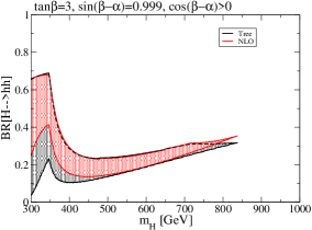
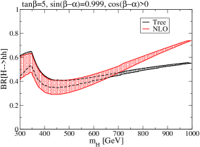
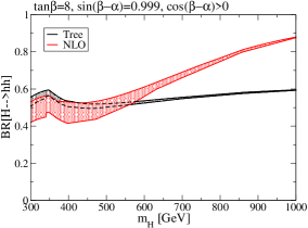
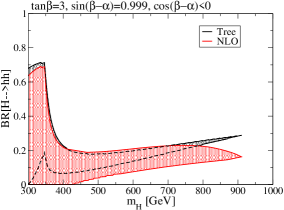
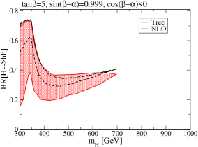
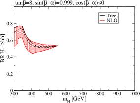
Figure 2: BR of the $H\to hh$ decay with $\sin(\beta-\alpha)=0.999$ at NLO (red regions) and LO (black regions) in each value of $m_{H}(=m_{A}=m_{H^{\pm}})$ in the Type-I THDM. From left to right panels, the value of $\tan\beta$ are fixed to be 3, 5, and 8. Upper panels and bottom panels show predictions with $\cos(\beta-\alpha)>0$ and $\cos(\beta-\alpha)<0$, respectively. We scan the value of $M^{2}$ in the range of $M^{2}\geq 0$ under the constraints of perturbative unitarity, vacuum stability and the $S$ and $T$ parameters.

V.1 Branching ratio of $H\to hh$

We first investigate the BR of the $H\to hh$ process. In order to see the structure of the loop corrections, we further simplify the approximate formula given in Eq. (81) in Sec. IV by taking degenerate masses of the additional Higgs bosons. In addition, for $m_{H}^{2}\gg m_{h}^{2}$, the bosonic loop contributions can be expanded as

$$\Delta_{0,B}^{\textrm{EW}} =\frac{\cot 2\beta}{16\pi^{2}}\frac{m_{H}^{4}}{v^{4}}\left(1-\frac{M^{2}}{m_{H}^{2}}\right)^{2}\Bigg{\{}24(1-C)\left(1-\frac{M^{2}}{m_{H}^{2}}\right)+6C$$

$$+\epsilon\left[8(2-3C)\left(1-\frac{M^{2}}{m_{H}^{2}}\right)+23-42C+3C\frac{m_{H}^{2}}{m_{H}^{2}-M^{2}}\right]+\mathcal{O}(\epsilon^{2})\Bigg{\}},$$ (98)

with $\epsilon\equiv m_{h}^{2}/m_{H}^{2}$ and $C\equiv 2-\pi/\sqrt{3}\simeq 0.186$. From this approximate formula, it is seen that $\Delta_{0,B}^{\textrm{EW}}$ is enhanced by $m_{H}^{4}$ for the case with $M\ll m_{H}$ due to the non-decoupling effect. On the other hand, for $M\simeq m_{H}$ such an enhancement is highly suppressed by the factor of $(1-M^{2}/m_{H}^{2})^{2}$ and thus $\Delta_{0,B}^{\textrm{EW}}$ is roughly proportional to $(m_{H}^{2}-M^{2})^{2}/v^{4}$. It can also be seen that Eq. (98) has the factor $\cot 2\beta$, so that the magnitude of the NLO corrections grows as $\tan\beta$ increases. We note that the NLO contributions come from the cross term of the amplitude from the tree level and one-loop contributions, so that the sign of the NLO contributions changes depending on the sign of $c_{\beta-\alpha}$. Namely, if $c_{\beta-\alpha}$ is positive (negative), the NLO contributions increase (decrease) the decay rate. Features of the loop corrections as those described here can be concretely confirmed by the following Figs. 2 and 3.

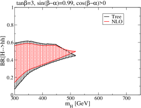
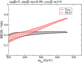
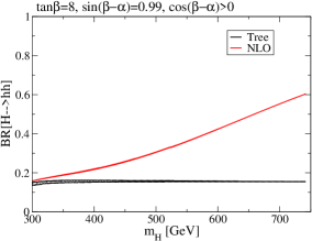
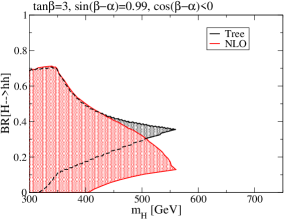
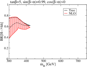
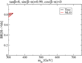
Figure 3: Same as Fig. 2, but for $\sin(\beta-\alpha)=0.99$.

Fig. 2 shows the $m_{H}$ dependence of the BR of $H\to hh$ including the NLO corrections (red regions) and that at tree level (black regions) for the degenerate mass case; i.e., $m_{H}=m_{A}=m_{H^{\pm}}$. We fix $s_{\beta-\alpha}=0.999$, where the upper panels (the lower panels) represent results with $c_{\beta-\alpha}>0$ ($c_{\beta-\alpha}<0$). Results for $\tan\beta=3$, 5 and 8 are shown from the left panels to the right panels. We scan the parameter $M^{2}$ within $M^{2}\geq 0$ in each value of $m_{H}$. In the case with $c_{\beta-\alpha}>0$, it can be confirmed that the NLO corrections typically increase the BR, which tends to be clearer at large $\tan\beta$ and/or large mass regions. For $c_{\beta-\alpha}<0$, the NLO corrections typically decrease the BR. We note that the parameter regions where the non-decoupling quantum effects are important are excluded by the perturbative unitarity bound. The value of the BR drops sharply at around $m_{H}=350$ GeV because the $H\to t\bar{t}$ process opens.

Fig. 3 shows the decay BR of $H\to hh$ in the case with $s_{\beta-\alpha}=0.99$, while the other configurations are the same as those in Fig. 2. As compared with the case for $s_{\beta-\alpha}=0.999$, the BR typically becomes smaller values and the upper limit on $m_{H}$ is stronger due to the theoretical constraints.

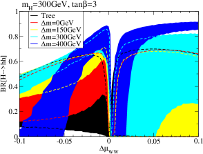
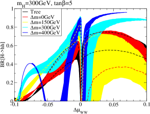
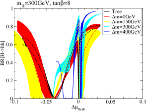
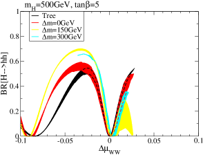
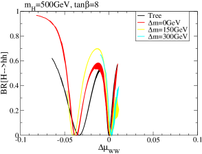
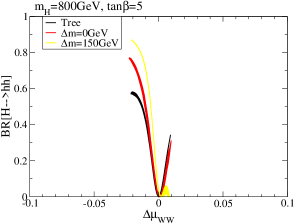
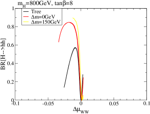
Figure 4: Correlation between the BR of $H\to hh$ and the deviation in the ratio of the branching ratio of $h\to WW^{*}$ from the SM prediction in the Type-I THDM. Black regions are predictions at tree level, while red, yellow, cyan and blue regions express predictions with the NLO corrections in the case with $\Delta m~{}(\equiv m_{A}-m_{H})=$ 0, 150 GeV, 300 GeV and 400 GeV, respectively. Top, middle and bottom panels show results where $m_{H}$ is fixed to be 300 GeV, 500 GeV and 800 GeV, respectively. From the panel of the left, the value of $\tan\beta$ is fixed to be 3, 5, and 8. We scan the value of $M^{2}$ and $\cos(\beta-\alpha)$ under the constraints of perturbative unitarity, vacuum stability and the $S$ and $T$ parameters.

Next, we investigate the correlation between the BR of $H\to hh$ and the BR of $h\to WW^{*}\to Wf\bar{f}^{\prime}$ which is expected to be measured with 2% accuracy at the ILC with the collision energy being 250 GeV Fujii:2017vwa . In order to parametrize the deviation in the BR of $h\to WW^{*}$ from the SM prediction, we introduce $\Delta\mu_{WW}$ defined as

$$\Delta\mu_{WW}\equiv\frac{\textrm{BR}[h\to WW^{*}]_{\textrm{THDM}}}{\textrm{BR}[h\to WW^{*}]_{\textrm{SM}}}-1,$$ (99)

where $\textrm{BR}[h\to WW^{*}]_{\textrm{THDM}}$ ($\textrm{BR}[h\to WW^{*}]_{\textrm{SM}}$) represents the BR in the THDM (SM). We numerically evaluate the value of $\Delta\mu_{WW}$ by using H-COUP Kanemura:2019slf .

In Fig. 4, we show the correlation between the BR of the $H\to hh$ process and $\Delta\mu_{WW}$ for each fixed value of $\tan\beta$ and $m_{H}$. The values of $s_{\beta-\alpha}$ and $M^{2}$ are scanned under the constraints of perturbative unitarity, vacuum stability and data of the $S$ and $T$ oblique parameters. The regions shaded in black show the results at LO, while those shaded in red, yellow, cyan and blue show the results at NLO with the mass difference $\Delta m=m_{A}-m_{H}$ to be 0, 150, 300 and 400 GeV, respectively. In some of the panels, several colored regions do not appear because of no allowed region by the constraints. Results with $\Delta\mu_{WW}<0$ ($\Delta\mu_{WW}>0$) correspond to those with $c_{\beta-\alpha}>0$ ($c_{\beta-\alpha}<0$), because the partial decay width of $h\to b\bar{b}$ is enhanced (suppressed). In the case with heavier $H$, predictions are well determined to be narrower regions, because the allowed range of $M^{2}$ by the theoretical constraints is shrunk. It is seen that for $\Delta m=0$ and $\Delta\mu_{WW}<0$ ($\Delta\mu_{WW}>0$) , the value of the BR is pushed up (down) by the NLO corrections, in which this behavior can be understood from Eq. (98) and is consistent with the results shown in Figs. 2 and 3. It can also be seen that if the value of $\tan\beta$ increases, the NLO corrections increase, because bosonic-loop effects are proportional to $\cot 2\beta$ in Eq. (98). For $\Delta\mu_{WW}<0$; i.e., $c_{\beta-\alpha}>0$, the BR becomes 0 at particular values of $\Delta\mu_{WW}$; e.g., at around $\Delta\mu_{WW}=-0.4$ for $m_{H}=300$ GeV and $\tan\beta=8$. Such behavior can be explained by the expression of the tree level $Hhh$ coupling $\lambda_{Hhh}$ as given in Eqs. (25) and (27).

In the case with non-zero mass difference among additional Higgs bosons; i.e., $\Delta m\neq 0$, the behavior of loop corrections can drastically be different from that in case with $\Delta m=0$. As $\Delta m$ increases, the difference from the tree level prediction becomes more significant than that in the degenerate mass case. For results of $m_{H}=300$ GeV, predictions including the NLO corrections can be about 30 % larger than tree level predictions if $\Delta m$ is larger than 300 GeV. If $\Delta m$ is non-zero, the effect of NLO corrections can increase the BR in the both cases with $c_{\beta-\alpha}>0$ and $c_{\beta-\alpha}<0$. However, due to theoretical constraints, allowed regions become smaller as $m_{H}$ increases.

If $\Delta\mu_{WW}$ is larger than 2%, it can be observed as a deviation from the SM prediction by the precision measurements at the ILC with the center of mass energy $\sqrt{s}$ to be 250 GeV Fujii:2017vwa . However, even if the deviation of the $h\to WW^{*}$ decay is too small to be observed by the ILC, it might be possible to explore $H$ via the $H\to hh$ process at the HL-LHC. If $H$ is lighter than $2m_{t}$ and $\Delta m$ is non-zero, the $H\to hh$ decay mode can be dominant in large parameter regions.

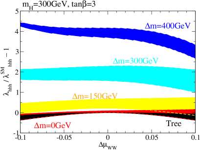
Figure 5: Correlation between BR($H\to hh$) and $\Delta\mu_{WW}$ (left panel) and that between BR($H\to hh$) and $\lambda_{hhh}/\lambda_{hhh}^{\textrm{SM}}-1$ (right panel) for $m_{H}=300$ GeV and $\tan\beta=3$. The color definitions of the regions are the same as specified in Fig. 4. We scan the value of $M^{2}$ and $\cos(\beta-\alpha)$ under the constraints of perturbative unitarity, vacuum stability and the $S$ and $T$ parameters. For the $hhh$ vertex, the renormalization scale is also taken as $\mu=m_{H}$ in the same as that for $\Gamma[H\to hh]$.

It is known that similar non-decoupling effects also appear in the loop corrected $hhh$ coupling Kanemura:2004mg ; Kanemura:2015mxa ; Kanemura:2017wtm . The physics of the $hhh$ coupling is strongly related with the EW baryogenesis, because the strong first order phase transition can lead to a large deviation in the $hhh$ coupling from the SM prediction at zero temperature Kanemura:2002vm ; Kanemura:2004ch ; Grojean:2004xa ; Braathen:2019zoh ; Braathen:2020vwo . The $hhh$ coupling can be extracted from the measurements of the double-Higgs production at hadron, lepton and photon colliders as discussed in Ref. Asakawa:2010xj . The measurement accuracy of the $hhh$ coupling is expected to be about 27% at the ILC with $\sqrt{s}=500$ GeV Fujii:2017vwa . In Fig. 5, we show the correlation between $\Delta\mu_{WW}$ and the deviation in the renormalized $hhh$ vertex in the Type-I THDM from that in the SM, in the case with $m_{H}=300$ GeV and $\tan\beta=3$. We calculate the renormalized $hhh$ vertex using H-COUP Kanemura:2017gbi ; Kanemura:2019slf , excepting parameter regions causing BR($H\to hh$)$<0$. The color definitions of the regions are the same as specified in Fig. 4. In order to examine the correlation with the BR of $H\to hh$, we also place the panel which is shown in Fig. 4. It can be seen that the deviation of the $hhh$ coupling is almost determined by the magnitude of $\Delta m$. The larger $\Delta m$ causes the larger deviation in the $hhh$ coupling, since it is caused by a larger non-decoupling effect. Namely, the structure of the non-decoupling effects is the same as those of the $H\to hh$ decay. Such parameter regions are common with regions where the $hhh$ coupling shifts from the SM predictions significantly so that the $H\to hh$ search at the HL-LHC might also be used to test the EW baryogenesis scenario multi-directionally.

V.2 Branching ratios of $H$

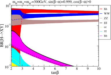
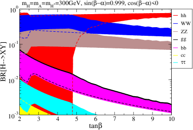
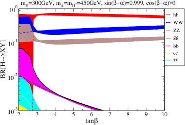
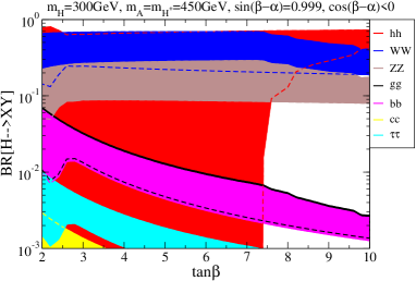
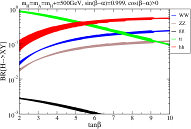
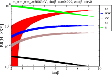
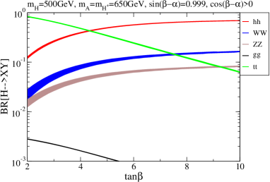
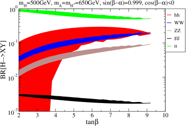
Figure 6: Branching ratios for $H$ as a function of $\tan\beta$ in the case of $\sin(\beta-\alpha)=0.999$ with $\cos(\beta-\alpha)>0$ (left panels) and $\cos(\beta-\alpha)<0$ (right panels). The upper four and lower four panels show the case with $m_{H}=300$ GeV and 500 GeV, respectively. The first and third (second and fourth) panels from the top show the case with $\Delta m$ ($=m_{A}-m_{H^{\pm}}$) $=0$ (150 GeV). The value of $M^{2}$ is scanned under the constraints of perturbative unitarity, vacuum stability and the $S$ and $T$ parameters.

Finally, we investigate the other decay modes of $H$ in the Type-I THDM. In Fig. 6, we show the decay BRs for $H$ as a function of $\tan\beta$ for $s_{\beta-\alpha}=0.999$ and $c_{\beta-\alpha}>0$ ($c_{\beta-\alpha}<0$) in the left (right) panels. We take $(m_{H},\Delta m)=(300,0)$ GeV, $(300,150)$ GeV, $(500,0)$ GeV and $(500,150)$ GeV from the top to the bottom panels. The value of $M^{2}$ is scanned with $M^{2}\geq 0$ in all the panels. As we can see in the panels for $m_{H}=300$ GeV, $H\to VV$ are the dominant decay modes. The BR of $H\to hh$ can also be dominant depending on the values of $M^{2}$ and $\tan\beta$. In the low $\tan\beta$ regions, the wider range of $M^{2}$ is allowed by the theoretical constraints, so that possible values of BR($H\to hh$) spread. For $\Delta m=150$ GeV and $c_{\beta-\alpha}>0$ ($c_{\beta-\alpha}<0$), the loop effects enhance (suppress) the decay rate of the $H\to hh$ process as compared with the case for $\Delta m=0$, so that BR($H\to hh$) tends to be more important than BR($H\to VV$). In the case with $m_{H}=500$ GeV, the $H\to t\bar{t}$ mode opens, whose decay rate is proportional to $\cot^{2}\beta$. Thus, the $H\to hh$ process becomes the main decay mode in the large $\tan\beta$ region. For $\Delta m=150$ GeV and $c_{\beta-\alpha}>0$, BR($H\to hh$) is typically enhanced with several tens of percent than that for $\Delta m=0$. On the other hand for $c_{\beta-\alpha}<0$, BR($H\to hh$) does not increase even if $\tan\beta$ becomes large and/or $\Delta m$ is taken to be non-zero. Therefore, $H\to t\bar{t}$ is typically the main decay mode. We note that the search for heavy Higgs bosons decaying into $t\bar{t}$ at hadron colliders is challenging due to the large the SM background, but various simulation studies for detecting such Higgs bosons have been done at LHC in Refs. Craig:2015jba ; Bernreuther:2015fts ; Kanemura:2015nza ; Djouadi:2016ack ; Hespel:2016qaf ; Carena:2016npr ; Bernreuther:2017yhg ; BuarqueFranzosi:2017jrj ; Adhikary:2018ise ; Djouadi:2019cbm ; Bahl:2020kwe .

VI Discussions

We discuss the direct search for the additional Higgs bosons at future collider experiments. At the HL-LHC, $H$ or $A$ is mainly produced by the gluon fusion process and the associated production with $b\bar{b}$.  The parameter region expected to be explored via these single productions has been studied in Ref. Aiko:2020ksl , where the analysis has been done at LO in the EW interaction. It goes without saying that the search for the additional Higgs bosons can also be done at the ILC energy upgrade, where the collision energy $\sqrt{s}$ can be extended to be up to 1 TeV Baer:2013cma . They can mainly be produced in pairs as $e^{+}e^{-}\to HA$ and $e^{+}e^{-}\to H^{+}H^{-}$ up to 500 GeV for the degenerate mass case. As we have shown in this paper, the BRs of $H$ can significantly be changed by the NLO corrections in EW and scalar interactions. Thus, it is quite important to include such effects in the exploration of the additional Higgs bosons at the HL-LHC and the ILC. We will upgrade the numerical program H-COUP Kanemura:2017gbi ; Kanemura:2019slf such that the decay BRs for the additional Higgs bosons are calculated including EW, scalar and QCD corrections based on this paper ($H$), Ref. Aiko:2022XX ($A$) and Ref. Aiko:2021can ($H^{\pm}$). We will then be able to discuss the synergy between the direct search and the precise measurement of $h$, which will be left for future works.

Finally, we would like to comment that a portion of the parameter space shown in our numerical results is excluded by the current experimental data from the additional Higgs boson searches at LHC and the measurement of the signal strength of $h$ given in Sec. II. For example, the region $\Delta\mu_{WW}\lesssim 0$ are excluded by taking into account the constraints on $\alpha$ and $\beta$ in the THDMs from the signal strength data ATLAS:2021vrm . It is, however, seen that there is a large discrepancy between the region excluded by the observed data and that by the expectation of the MonteCarlo analysis. Thus, the observed exclusion can be drastically changed by accumulating more data. Therefore, we have investigated wider regions of the parameter space than the allowed ones by the current experimental data in the numerical calculations.

VII Conclusions

We have computed the decay rates of the additional CP-even Higgs boson $H$; i.e., $H\to hh$, $H\to f\bar{f}$ and $H\to VV$ with the EW and scalar NLO corrections in the THDMs with a softly broken $Z_{2}$ symmetry, where QCD corrections are also included for $H\to q\bar{q}$. For loop induced processes, we have calculated the decay rates at LO in EW and scalar interactions, but including QCD corrections. We have particularly focused on the scenario with the nearly alignment in the Type-I THDM for numerical evaluations. We have clarified that various parameter dependences such as $\tan\beta$, $m_{H}$, $\Delta m(=m_{A}-m_{H})$ and the sign of $c_{\beta-\alpha}$ on the BR of $H\to hh$ under the constraints from perturbative unitarity, vacuum stability and electroweak precision data. It has been found that the effect of the radiative corrections on the BR of $H\to hh$ can drastically change its LO prediction due to the non-decoupling effect of the additional Higgs boson loops. We have also investigated the correlation between the deviation in the BR of $h\to WW^{*}$ from the SM prediction ($\Delta\mu_{WW}$) and the BR of $H\to hh$ at NLO in EW and scalar interactions. For example, in the case with $m_{H}=500$ GeV and $\tan\beta=3$ and $\Delta\mu_{WW}=0.05$, BR($H\to hh$) can be 0.3-0.4, 0.1-0.4, 0-0.25 and 0.3-0.35 at LO, at NLO with $\Delta m=0$, 150 GeV and 300 GeV, respectively. Even if $|\Delta\mu_{WW}|$ is less than 0.02 which might not be able to be detected at the ILC, we have seen that the $H\to hh$ can be the dominant decay mode; e.g., BR($H\to hh$) can be about 70 % for $m_{H}=500$ GeV, $\Delta m=300$ GeV and $\tan\beta=5$. Therefore, it has been shown that including the radiative corrections to the decay of $H$ is quite important for the direct searches for the additional Higgs bosons at future collider experiments such as the HL-LHC and the ILC.

Appendix A One-loop diagrams for the renormalized $Hhh$ vertex

We present analytic formulae of one-loop diagrams related with the renormalized $Hhh$ vertex. All feynman diagrams are computed in the ’t Hooft-Feynman gauge, and are expressed by Passarino Veltman functions Passarino:1978jh .

Two-point functions include not only 1PI contributions $\Pi_{h_{i}h_{j}}^{\textrm{1PI}}$ but also pinch terms $\Pi_{h_{i}h_{j}}^{\textrm{PT}}$ and tadpole contributions $\Pi_{h_{i}h_{j}}^{\textrm{Tad}}$. For two-point functions of scalar fields, explicit formulae of $\Pi_{h_{i}h_{j}}^{\textrm{1PI}}$ and those of $\Pi_{h_{i}h_{j}}^{\textrm{PT}}$ are given in Ref. Kanemura:2015mxa and in Ref. Kanemura:2017wtm , respectively. The contributions $\Pi_{h_{i}h_{j}}^{\textrm{Tad}}$ are calculated as

$$\Pi_{hh}^{\textrm{Tad}}=\frac{6\lambda_{hhh}}{m_{h}^{2}}T_{h}^{\textrm{1PI}}+\frac{2\lambda_{Hhh}}{m_{H}^{2}}T_{H}^{\textrm{1PI}},$$ (100)

$$\Pi_{HH}^{\textrm{Tad}}=\frac{2\lambda_{HHh}}{m_{h}^{2}}T_{h}^{\textrm{1PI}}+\frac{6\lambda_{HHH}}{m_{H}^{2}}T_{H}^{\textrm{1PI}},$$ (101)

$$\Pi_{Hh}^{\textrm{Tad}}=\frac{2\lambda_{Hhh}}{m_{h}^{2}}T_{h}^{\textrm{1PI}}+\frac{2\lambda_{HHh}}{m_{H}^{2}}T_{H}^{\textrm{1PI}},$$ (102)

$$\Pi_{AG}^{\textrm{Tad}}=\frac{\lambda_{hGA}}{m_{h}^{2}}T_{h}^{\textrm{1PI}}+\frac{\lambda_{HGA}}{m_{H}^{2}}T_{H}^{\textrm{1PI}},$$ (103)

where explicit formulae of $T_{h_{i}}^{\textrm{1PI}}$ are given in Ref. Kanemura:2015mxa .

Contributions of one-loop diagrams for the three-point vertex $Hhh$ are also composed by 1PI diagram contributions and tadpole contributions as

$$\Gamma_{Hhh}[p_{1}^{2},p_{2}^{2},q^{2}]=\Gamma_{Hhh}^{\textrm{1PI}}[p_{1}^{2},p_{2}^{2},q^{2}]+\Gamma_{Hhh}^{\textrm{Tad}},$$ (104)

where $p_{1}^{\mu}$ and $p_{2}^{\mu}$ are the incoming momenta of two 125 GeV Higgs bosons $h$, and $q^{\mu}(=p_{1}^{\mu}+p_{2}^{\mu})$ is the outgoing momentum of $H$. Tadpole contributions to the $Hhh$ vertex are given as

$$\Gamma_{Hhh}^{\textrm{Tad}}=6\frac{\lambda_{Hhhh}}{m_{h}^{2}}T_{h}^{\textrm{1PI}}+4\frac{\lambda_{HHhh}}{m_{H}^{2}}T_{H}^{\textrm{1PI}}.$$ (105)

Fermionic loop contributions and bosonic loop contributions for the 1PI diagrams are respectively calculated as

$$\Gamma_{Hhh}^{\textrm{1PI}}[p_{1}^{2},p_{2}^{2},q^{2}]_{F}=-\sum_{f}\frac{8m_{f}^{4}N_{c}^{f}}{16\pi^{2}v^{3}}(\kappa_{f}^{f})^{2}\kappa_{f}^{H}\big{[}B_{0}[p_{1}^{2};f,f]+B_{0}[p_{2}^{2};f,f]+B_{0}[q^{2};f,f]$$

$$+(4m_{f}^{2}-q^{2}+p_{1}\cdot p_{2})C_{0}[f,f,f]\big{]},$$ (106)

and

$$(16\pi^{2})\Gamma_{Hhh}^{\textrm{1PI}}[p_{1}^{2},p_{2}^{2},q^{2}]_{B}$$

$$=\frac{g_{Z}^{3}m_{Z}}{4}\Big{(}s_{\beta-\alpha}^{2}c_{\beta-\alpha}C^{\phi\phi\phi}_{VVS}[Z,Z,A]-c_{\beta-\alpha}^{3}C^{\phi\phi\phi}_{VSV}[Z,A,Z]+s_{\beta-\alpha}^{2}c_{\beta-\alpha}C_{SVV}^{\phi\phi\phi}[A,Z,Z]$$

$$-s_{\beta-\alpha}^{2}c_{\beta-\alpha}C_{VVS}^{\phi\phi\phi}[Z,Z,G^{0}]-s_{\beta-\alpha}^{2}c_{\beta-\alpha}C_{VSV}^{\phi\phi\phi}[Z,G^{0},Z]-s_{\beta-\alpha}^{2}c_{\beta-\alpha}C_{SVV}^{\phi\phi\phi}[G^{0},Z,Z]\Big{)}$$

$$+\frac{g^{3}m_{W}}{2}\Big{(}s_{\beta-\alpha}^{2}c_{\beta-\alpha}C_{VVS}^{\phi\phi\phi}[W,W,H^{\pm}]-c_{\beta-\alpha}^{3}C_{VSV}^{\phi\phi\phi}[W,H^{\pm},W]+s_{\beta-\alpha}^{2}c_{\beta-\alpha}C_{SVV}^{\phi\phi\phi}[H^{\pm},W,W]$$

$$-s_{\beta-\alpha}^{2}c_{\beta-\alpha}C_{VVS}^{\phi\phi\phi}[W,W,G^{\pm}]-s_{\beta-\alpha}^{2}c_{\beta-\alpha}C_{VSV}^{\phi\phi\phi}[W,G^{\pm},W]-s_{\beta-\alpha}^{2}c_{\beta-\alpha}C_{SVV}^{\phi\phi\phi}[G^{\pm},W,W]\Big{)}$$

$$+\frac{g^{2}}{2}\Big{(}s_{\beta-\alpha}c_{\beta-\alpha}\lambda_{hG^{+}G^{-}}C_{VSS}^{\phi\phi\phi}[W,G^{\pm},G^{\pm}]+s_{\beta-\alpha}^{2}\lambda_{HG^{+}G^{-}}C_{SVS}^{\phi\phi\phi}[G^{\pm},W,G^{\pm}]$$

$$+s_{\beta-\alpha}c_{\beta-\alpha}\lambda_{hG^{+}G^{-}}C_{SSV}^{\phi\phi\phi}[G^{\pm},G^{\pm},W]-s_{\beta-\alpha}c_{\beta-\alpha}\lambda_{hH^{+}H^{-}}C_{VSS}^{\phi\phi\phi}[W,H^{\pm},H^{\pm}]$$

$$+c_{\beta-\alpha}^{2}\lambda_{HH^{+}H^{-}}C_{SVS}^{\phi\phi\phi}[H^{\pm},W,H^{\pm}]-s_{\beta-\alpha}c_{\beta-\alpha}\lambda_{hH^{+}H^{-}}C_{SSV}^{\phi\phi\phi}[H^{\pm},H^{\pm},W]$$

$$+c_{\beta-\alpha}^{2}\lambda_{hG^{+}H^{-}}C_{VSS}^{\phi\phi\phi}[W,H^{\pm},G^{\pm}]+s_{\beta-\alpha}c_{\beta-\alpha}\lambda_{HG^{+}H^{-}}C_{SVS}^{\phi\phi\phi}[H^{\pm},W,G^{\pm}]$$

$$-s_{\beta-\alpha}^{2}\lambda_{hG^{+}H^{-}}C_{SSV}^{\phi\phi\phi}[H^{\pm},G^{\pm},W]-s_{\beta-\alpha}^{2}\lambda_{hG^{+}H^{-}}C_{VSS}^{\phi\phi\phi}[W,G^{\pm},H^{\pm}]$$

$$+s_{\beta-\alpha}c_{\beta-\alpha}\lambda_{HG^{+}H^{-}}C_{SVS}^{\phi\phi\phi}[G^{\pm},W,H^{\pm}]+c_{\beta-\alpha}^{2}\lambda_{hG^{+}H^{-}}C_{SSV}^{\phi\phi\phi}[G^{\pm},H^{\pm},W]\Big{)}$$

$$+\frac{g_{Z}^{2}}{2}\Big{(}-s_{\beta-\alpha}c_{\beta-\alpha}\lambda_{hAA}C_{VSS}^{\phi\phi\phi}[Z,A,A]+c_{\beta-\alpha}^{2}\lambda_{HAA}C_{SVS}^{\phi\phi\phi}[A,Z,A]-s_{\beta-\alpha}c_{\beta-\alpha}\lambda_{hAA}C_{SSV}^{\phi\phi\phi}[A,A,Z]$$

$$+s_{\beta-\alpha}c_{\beta-\alpha}\lambda_{hG^{0}G^{0}}C_{VSS}^{\phi\phi\phi}[Z,G^{0},G^{0}]+s_{\beta-\alpha}^{2}\lambda_{HG^{0}G^{0}}C_{SVS}^{\phi\phi\phi}[G^{0},Z,G^{0}]+s_{\beta-\alpha}c_{\beta-\alpha}\lambda_{hG^{0}G^{0}}C_{SSV}^{\phi\phi\phi}[G^{0},G^{0},Z]\Big{)}$$

$$+\frac{g_{Z}^{2}}{4}\Big{(}c_{\beta-\alpha}^{2}\lambda_{hG^{0}A}C_{VSS}^{\phi\phi\phi}[Z,A,G^{0}]+s_{\beta-\alpha}c_{\beta-\alpha}\lambda_{HG^{0}A}C_{SVS}^{\phi\phi\phi}[A,Z,G^{0}]-s_{\beta-\alpha}^{2}\lambda_{hG^{0}A}C_{SSV}^{\phi\phi\phi}[A,G^{0},Z]$$

$$-s_{\beta-\alpha}^{2}\lambda_{hG^{0}A}C_{VSS}^{\phi\phi\phi}[Z,G^{0},A]+s_{\beta-\alpha}c_{\beta-\alpha}\lambda_{HG^{0}A}C_{SVS}^{\phi\phi\phi}[G^{0},Z,A]+c_{\beta-\alpha}^{2}\lambda_{hG^{0}A}C_{SSV}^{\phi\phi\phi}[G^{0},A,Z]\Big{)}$$

$$+\frac{g^{3}m_{W}^{3}}{2}s_{\beta-\alpha}^{2}c_{\beta-\alpha}\left(16C_{0}[W,W,W]-C_{0}[c^{\pm},c^{\pm},c^{\pm}]\right)+\frac{g_{Z}^{3}m_{Z}^{3}}{4}s_{\beta-\alpha}^{2}c_{\beta-\alpha}\left(16C_{0}[Z,Z,Z]-C_{0}[c_{Z},c_{Z},c_{Z}]\right)$$

$$-72\lambda_{hhh}^{2}\lambda_{Hhh}C_{0}[h,h,h]-24\lambda_{hhh}\lambda_{Hhh}\lambda_{HHh}(C_{0}[H,h,h]+C_{0}[h,h,H])-8\lambda_{Hhh}^{3}C_{0}[h,H,h]$$

$$-8\lambda_{HHh}^{2}\lambda_{Hhh}(C_{0}[H,H,h]+C_{0}[h,H,H])-24\lambda_{HHH}\lambda_{Hhh}^{2}C_{0}[H,h,H]-24\lambda_{HHH}\lambda_{HHh}^{2}C_{0}[H,H,H]$$

$$-8\lambda_{HAA}\lambda_{hAA}^{2}C_{0}[A,A,A]-2\lambda_{HG^{0}A}\lambda_{hG^{0}A}\lambda_{hG^{0}G^{0}}(C_{0}[A,G^{0},G^{0}]+C_{0}[G^{0},G^{0},A])$$

$$-8\lambda_{HG^{0}G^{0}}\lambda_{hG^{0}G^{0}}^{2}C_{0}[G^{0},G^{0},G^{0}]-2\lambda_{HG^{0}G^{0}}\lambda_{hG^{0}A}^{2}C_{0}[G^{0},A,G^{0}]$$

$$-2\lambda_{HG^{0}A}\lambda_{hAA}\lambda_{hG^{0}A}(C_{0}[A,A,G^{0}]+C_{0}[G^{0},A,A])-2\lambda_{HAA}\lambda_{hG^{0}A}^{2}C_{0}[A,G^{0},A]$$

$$-2\lambda_{HG^{+}G^{-}}\lambda_{hG^{+}G^{-}}^{2}C_{0}[G^{\pm},G^{\pm},G^{\pm}]-2\lambda_{HH^{+}H^{-}}\lambda_{hH^{+}H^{-}}^{2}C_{0}[H^{\pm},H^{\pm},H^{\pm}]$$

$$-2\lambda_{HG^{+}G^{-}}\lambda_{hG^{+}H^{-}}^{2}C_{0}[G^{\pm},H^{\pm},G^{\pm}]-2\lambda_{HG^{+}H^{-}}\lambda_{hG^{+}H^{-}}\lambda_{hG^{+}G^{-}}(C_{0}[H^{\pm},G^{\pm},G^{\pm}]+C_{0}[G^{\pm},G^{\pm},H^{\pm}])$$

$$-2\lambda_{HH^{+}H^{-}}\lambda_{hG^{+}H^{-}}^{2}C_{0}[H^{\pm},G^{\pm},H^{\pm}]-2\lambda_{HG^{+}H^{-}}\lambda_{hH^{+}H^{-}}\lambda_{hG^{+}H^{-}}(C_{0}[H^{\pm},H^{\pm},G^{\pm}]+C_{0}[G^{\pm},H^{\pm},H^{\pm}])$$

$$+24\lambda_{Hhh}\lambda_{hhhh}B_{0}[q^{2};h,h]+18\lambda_{hhh}\lambda_{Hhhh}(B_{0}[p_{1}^{2};h,h]+B_{0}[p_{2}^{2};h,h])$$

$$+12\lambda_{HHh}\lambda_{Hhhh}B_{0}[q^{2};H,h]+8\lambda_{Hhh}\lambda_{HHhh}(B_{0}[p_{1}^{2};H,h]+B_{0}[p_{2}^{2};H,h])$$

$$+12\lambda_{HHH}\lambda_{HHhh}B_{0}[q^{2};H,H]+6\lambda_{HHh}\lambda_{HHHh}(B_{0}[p_{1}^{2};H,H]+B_{0}[p_{2}^{2};H,H])$$

$$+4\lambda_{HAA}\lambda_{hhAA}B_{0}[q^{2};A,A]+2\lambda_{hAA}\lambda_{HhAA}(B_{0}[p_{1}^{2};A,A]+B_{0}[p_{2}^{2};A,A])$$

$$+4\lambda_{HG^{0}G^{0}}\lambda_{hhG^{0}G^{0}}B_{0}[q^{2};G^{0},G^{0}]+2\lambda_{hG^{0}G^{0}}\lambda_{HhG^{0}G^{0}}(B_{0}[p_{1}^{2};G^{0},G^{0}]+B_{0}[p_{2}^{2};G^{0},G^{0}])$$

$$+2\lambda_{HG^{0}A}\lambda_{hhG^{0}A}B_{0}[q^{2};G^{0},A]+\lambda_{hG^{0}A}\lambda_{HhG^{0}A}(B_{0}[p_{1}^{2};G^{0},A]+B_{0}[p_{2}^{2};G^{0},A])$$

$$+2\lambda_{HH^{+}H^{-}}\lambda_{hhH^{+}H^{-}}B_{0}[q^{2};H^{\pm},H^{\pm}]+\lambda_{hH^{+}H^{-}}\lambda_{HhH^{+}H^{-}}(B_{0}[p_{1}^{2};H^{\pm},H^{\pm}]+B_{0}[p_{2}^{2};H^{\pm},H^{\pm}])$$

$$+2\lambda_{HG^{+}G^{-}}\lambda_{hhG^{+}G^{-}}B_{0}[q^{2};G^{\pm},G^{\pm}]+\lambda_{hG^{+}G^{-}}\lambda_{HhG^{+}G^{-}}(B_{0}[p_{1}^{2};G^{\pm},G^{\pm}]+B_{0}[p_{2}^{2};G^{\pm},G^{\pm}])$$

$$+4\lambda_{HG^{+}H^{-}}\lambda_{hhG^{+}H^{-}}B_{0}[q^{2};H^{\pm},G^{\pm}]+2\lambda_{hG^{+}H^{-}}\lambda_{HhG^{+}H^{-}}(B_{0}[p_{1}^{2};H^{\pm},G^{\pm}]+B_{0}[p_{2}^{2};H^{\pm},G^{\pm}])$$

$$+g^{3}m_{W}c_{\beta-\alpha}(2B_{0}[q^{2};W,W]-1)+\frac{g_{Z}^{3}m_{Z}}{2}c_{\beta-\alpha}(2B_{0}[q^{2};Z,Z]-1),$$ (107)

where definitions of combinations of $C$-functions are given as

$$C_{SVV}^{\phi\phi\phi}[S,V_{1},V_{2}] =[p_{1}^{2}C_{21}+p_{2}^{2}C_{22}+2p_{1}\cdot p_{2}C_{23}+4C_{24}-\frac{1}{2}$$

$$-(q+p_{1})\cdot(p_{1}C_{11}+p_{2}C_{12})+q\cdot p_{1}C_{0}](S,V_{1},V_{2}),$$ (108)

$$C_{VSV}^{\phi\phi\phi}[V_{2},S,V_{1}] =[p_{1}^{2}C_{21}+p_{2}^{2}C_{22}+2p_{1}\cdot p_{2}C_{23}+4C_{24}-\frac{1}{2}$$

$$+(3p_{1}-p_{2})\cdot(p_{1}C_{11}+p_{2}C_{12})+2p_{1}\cdot(p_{1}-p_{2})C_{0}](V_{2},S,V_{1}),$$ (109)

$$C_{VVS}^{\phi\phi\phi}[V_{1},V_{2},S] =[p_{1}^{2}C_{21}+p_{2}^{2}C_{22}+2p_{1}\cdot p_{2}C_{23}+4C_{24}-\frac{1}{2}$$

$$+(3p_{1}+4p_{2})\cdot(p_{1}C_{11}+p_{2}C_{12})+2q\cdot(q+p_{2})C_{0}](V_{1},V_{2},S),$$ (110)

$$C_{VSS}^{\phi\phi\phi}[V,S_{1},S_{2}] =[p_{1}^{2}C_{21}+p_{2}^{2}C_{22}+2p_{1}\cdot p_{2}C_{23}+4C_{24}-\frac{1}{2}$$

$$+(4p_{1}+2p_{2})\cdot(p_{1}C_{11}+p_{2}C_{12})+4q\cdot p_{1}C_{0}](V,S_{1},S_{2}),$$ (111)

$$C_{SVS}^{\phi\phi\phi}[S_{2},V,S_{1}] =[p_{1}^{2}C_{21}+p_{2}^{2}C_{22}+2p_{1}\cdot p_{2}C_{23}+4C_{24}-\frac{1}{2}$$

$$+2p_{2}\cdot(p_{1}C_{11}+p_{2}C_{12})-p_{1}\cdot(p_{1}+2p_{2})C_{0}](S_{2},V,S_{1}),$$ (112)

$$C_{SSV}^{\phi\phi\phi}[S_{1},S_{2},V] =[p_{1}^{2}C_{21}+p_{2}^{2}C_{22}+2p_{1}\cdot p_{2}C_{23}+4C_{24}-\frac{1}{2}$$

$$-2p_{2}\cdot(p_{1}C_{11}+p_{2}C_{12})-q\cdot(p_{1}-p_{2})C_{0}](S_{1},S_{2},V),$$ (113)

with

$$C_{i}[X,Y,Z]\equiv C_{i}[p_{1}^{2},p_{2}^{2},q^{2};m_{X},m_{Y},m_{Z}].$$ (114)

References

- (1) ATLAS collaboration, Observation of a new particle in the search for the Standard Model Higgs boson with the ATLAS detector at the LHC, Phys. Lett. B 716 (2012) 1 [1207.7214].
- (2) CMS collaboration, Observation of a New Boson at a Mass of 125 GeV with the CMS Experiment at the LHC, Phys. Lett. B 716 (2012) 30 [1207.7235].
- (3) ATLAS collaboration, Combined measurements of Higgs boson production and decay using up to fb-1 of proton-proton collision data at 13 TeV collected with the ATLAS experiment, Phys. Rev. D 101 (2020) 012002 [1909.02845].
- (4) CMS collaboration, Combined Higgs boson production and decay measurements with up to 137 fb-1 of proton-proton collision data at = 13 TeV, .
- (5) S. Kanemura, K. Tsumura, K. Yagyu and H. Yokoya, Fingerprinting nonminimal Higgs sectors, Phys. Rev. D 90 (2014) 075001 [1406.3294].
- (6) S. Kanemura, Y. Okada, E. Senaha and C.P. Yuan, Higgs coupling constants as a probe of new physics, Phys. Rev. D 70 (2004) 115002 [hep-ph/0408364].
- (7) S. Kanemura, M. Kikuchi and K. Yagyu, Radiative corrections to the Yukawa coupling constants in two Higgs doublet models, Phys. Lett. B 731 (2014) 27 [1401.0515].
- (8) S. Kanemura, M. Kikuchi and K. Yagyu, Fingerprinting the extended Higgs sector using one-loop corrected Higgs boson couplings and future precision measurements, Nucl. Phys. B 896 (2015) 80 [1502.07716].
- (9) S. Kanemura, M. Kikuchi, K. Sakurai and K. Yagyu, Gauge invariant one-loop corrections to higgs boson couplings in non-minimal higgs models, Phys. Rev. D 96 (2017) 035014 [1705.05399].
- (10) S. Kanemura, M. Kikuchi, K. Mawatari, K. Sakurai and K. Yagyu, Loop effects on the Higgs decay widths in extended Higgs models, Phys. Lett. B 783 (2018) 140 [1803.01456].
- (11) S. Kanemura, M. Kikuchi, K. Mawatari, K. Sakurai and K. Yagyu, Full next-to-leading-order calculations of Higgs boson decay rates in models with non-minimal scalar sectors, Nucl. Phys. B 949 (2019) 114791 [1906.10070].
- (12) M. Krause, R. Lorenz, M. Muhlleitner, R. Santos and H. Ziesche, Gauge-independent Renormalization of the 2-Higgs-Doublet Model, JHEP 09 (2016) 143 [1605.04853].
- (13) M. Krause, M. Muhlleitner, R. Santos and H. Ziesche, Higgs-to-Higgs boson decays in a 2HDM at next-to-leading order, Phys. Rev. D 95 (2017) 075019 [1609.04185].
- (14) M. Krause and M. Mühlleitner, Impact of Electroweak Corrections on Neutral Higgs Boson Decays in Extended Higgs Sectors, JHEP 04 (2020) 083 [1912.03948].
- (15) A. Arhrib, M. Capdequi Peyranere, W. Hollik and S. Penaranda, Higgs decays in the two Higgs doublet model: Large quantum effects in the decoupling regime, Phys. Lett. B 579 (2004) 361 [hep-ph/0307391].
- (16) M. Cepeda et al., Report from Working Group 2: Higgs Physics at the HL-LHC and HE-LHC, CERN Yellow Rep. Monogr. 7 (2019) 221 [1902.00134].
- (17) H. Baer et al., The International Linear Collider Technical Design Report - Volume 2: Physics, 1306.6352.
- (18) K. Fujii et al., Physics Case for the 250 GeV Stage of the International Linear Collider, 1710.07621.
- (19) S. Asai, J. Tanaka, Y. Ushiroda, M. Nakao, J. Tian, S. Kanemura et al., Report by the Committee on the Scientific Case of the ILC Operating at 250 GeV as a Higgs Factory, 1710.08639.
- (20) LCC Physics Working Group collaboration, Tests of the Standard Model at the International Linear Collider, 1908.11299.
- (21) M. Ahmad et al., CEPC-SPPC Preliminary Conceptual Design Report. 1. Physics and Detector, .
- (22) TLEP Design Study Working Group collaboration, First Look at the Physics Case of TLEP, JHEP 01 (2014) 164 [1308.6176].
- (23) S. Kanemura, M. Kikuchi, K. Sakurai and K. Yagyu, H-COUP: a program for one-loop corrected Higgs boson couplings in non-minimal Higgs sectors, Comput. Phys. Commun. 233 (2018) 134 [1710.04603].
- (24) S. Kanemura, M. Kikuchi, K. Mawatari, K. Sakurai and K. Yagyu, H-COUP Version 2: a program for one-loop corrected Higgs boson decays in non-minimal Higgs sectors, Comput. Phys. Commun. 257 (2020) 107512 [1910.12769].
- (25) M. Krause, M. Mühlleitner and M. Spira, 2HDECAY —A program for the calculation of electroweak one-loop corrections to Higgs decays in the Two-Higgs-Doublet Model including state-of-the-art QCD corrections, Comput. Phys. Commun. 246 (2020) 106852 [1810.00768].
- (26) A. Denner, S. Dittmaier and A. Mück, PROPHECY4F 3.0: A Monte Carlo program for Higgs-boson decays into four-fermion final states in and beyond the Standard Model, Comput. Phys. Commun. 254 (2020) 107336 [1912.02010].
- (27) ATLAS collaboration, Search for heavy Higgs bosons decaying into two tau leptons with the ATLAS detector using collisions at TeV, Phys. Rev. Lett. 125 (2020) 051801 [2002.12223].
- (28) ATLAS collaboration, Search for heavy neutral Higgs bosons produced in association with -quarks and decaying into -quarks at TeV with the ATLAS detector, Phys. Rev. D 102 (2020) 032004 [1907.02749].
- (29) ATLAS collaboration, Search for heavy particles decaying into top-quark pairs using lepton-plus-jets events in proton–proton collisions at TeV with the ATLAS detector, Eur. Phys. J. C 78 (2018) 565 [1804.10823].
- (30) ATLAS collaboration, Search for pair production of Higgs bosons in the final state using proton-proton collisions at TeV with the ATLAS detector, JHEP 01 (2019) 030 [1804.06174].
- (31) ATLAS collaboration, Search for heavy resonances decaying into in the final state in collisions at TeV with the ATLAS detector, Eur. Phys. J. C 78 (2018) 24 [1710.01123].
- (32) ATLAS collaboration, Search for heavy resonances decaying into a pair of Z bosons in the and final states using 139 of proton–proton collisions at TeV with the ATLAS detector, Eur. Phys. J. C 81 (2021) 332 [2009.14791].
- (33) ATLAS collaboration, Search for resonances decaying into a weak vector boson and a Higgs boson in the fully hadronic final state produced in protonproton collisions at TeV with the ATLAS detector, Phys. Rev. D 102 (2020) 112008 [2007.05293].
- (34) ATLAS collaboration, Search for a heavy Higgs boson decaying into a Z boson and another heavy Higgs boson in the and final states in collisions at TeV with the ATLAS detector, Eur. Phys. J. C 81 (2021) 396 [2011.05639].
- (35) ATLAS collaboration, Search for charged Higgs bosons decaying into a top quark and a bottom quark at = 13 TeV with the ATLAS detector, JHEP 06 (2021) 145 [2102.10076].
- (36) CMS collaboration, Search for beyond the standard model Higgs bosons decaying into a pair in pp collisions at 13 TeV, JHEP 08 (2018) 113 [1805.12191].
- (37) CMS collaboration, Search for heavy Higgs bosons decaying to a top quark pair in proton-proton collisions at 13 TeV, JHEP 04 (2020) 171 [1908.01115].
- (38) CMS collaboration, Search for resonances in highly boosted lepton+jets and fully hadronic final states in proton-proton collisions at TeV, JHEP 07 (2017) 001 [1704.03366].
- (39) CMS collaboration, Search for a massive resonance decaying to a pair of Higgs bosons in the four b quark final state in proton-proton collisions at 13 TeV, Phys. Lett. B 781 (2018) 244 [1710.04960].
- (40) CMS collaboration, Search for a heavy Higgs boson decaying to a pair of W bosons in proton-proton collisions at 13 TeV, JHEP 03 (2020) 034 [1912.01594].
- (41) CMS collaboration, Search for a heavy pseudoscalar Higgs boson decaying into a 125 GeV Higgs boson and a Z boson in final states with two tau and two light leptons at 13 TeV, JHEP 03 (2020) 065 [1910.11634].
- (42) CMS collaboration, Search for charged Higgs bosons decaying into a top and a bottom quark in the all-jet final state of pp collisions at = 13 TeV, JHEP 07 (2020) 126 [2001.07763].
- (43) CMS collaboration, Search for charged Higgs bosons in the H± decay channel in proton-proton collisions at 13 TeV, JHEP 07 (2019) 142 [1903.04560].
- (44) J.F. Gunion and H.E. Haber, The CP conserving two Higgs doublet model: The Approach to the decoupling limit, Phys. Rev. D 67 (2003) 075019 [hep-ph/0207010].
- (45) N. Craig, J. Galloway and S. Thomas, Searching for Signs of the Second Higgs Doublet, 1305.2424.
- (46) M. Carena, I. Low, N.R. Shah and C.E.M. Wagner, Impersonating the Standard Model Higgs Boson: Alignment without Decoupling, JHEP 04 (2014) 015 [1310.2248].
- (47) H.E. Haber and O. Stål, New LHC benchmarks for the -conserving two-Higgs-doublet model, Eur. Phys. J. C 75 (2015) 491 [1507.04281].
- (48) J. Bernon, J.F. Gunion, H.E. Haber, Y. Jiang and S. Kraml, Scrutinizing the alignment limit in two-Higgs-doublet models: mh=125 GeV, Phys. Rev. D 92 (2015) 075004 [1507.00933].
- (49) B. Dumont, J.F. Gunion, Y. Jiang and S. Kraml, Constraints on and future prospects for Two-Higgs-Doublet Models in light of the LHC Higgs signal, Phys. Rev. D 90 (2014) 035021 [1405.3584].
- (50) N. Craig, F. D’Eramo, P. Draper, S. Thomas and H. Zhang, The Hunt for the Rest of the Higgs Bosons, JHEP 06 (2015) 137 [1504.04630].
- (51) J. Bernon, J.F. Gunion, H.E. Haber, Y. Jiang and S. Kraml, Scrutinizing the alignment limit in two-Higgs-doublet models. II. mH=125 GeV, Phys. Rev. D 93 (2016) 035027 [1511.03682].
- (52) D. Chowdhury and O. Eberhardt, Update of Global Two-Higgs-Doublet Model Fits, JHEP 05 (2018) 161 [1711.02095].
- (53) W. Su, M. White, A.G. Williams and Y. Wu, Exploring the low region of two Higgs doublet models at the LHC, 1909.09035.
- (54) F. Kling, S. Su and W. Su, 2HDM Neutral Scalars under the LHC, JHEP 06 (2020) 163 [2004.04172].
- (55) S. Kanemura, H. Yokoya and Y.-J. Zheng, Complementarity in direct searches for additional Higgs bosons at the LHC and the International Linear Collider, Nucl. Phys. B 886 (2014) 524 [1404.5835].
- (56) M. Aiko, S. Kanemura, M. Kikuchi, K. Mawatari, K. Sakurai and K. Yagyu, Probing extended Higgs sectors by the synergy between direct searches at the LHC and precision tests at future lepton colliders, Nucl. Phys. B 966 (2021) 115375 [2010.15057].
- (57) V.D. Barger, M.S. Berger, A.L. Stange and R.J.N. Phillips, Supersymmetric Higgs boson hadroproduction and decays including radiative corrections, Phys. Rev. D 45 (1992) 4128.
- (58) P. Osland and P.N. Pandita, Measuring the trilinear couplings of MSSM neutral Higgs bosons at high-energy e+ e- colliders, Phys. Rev. D 59 (1999) 055013 [hep-ph/9806351].
- (59) Y.P. Philippov, Yukawa Radiative Corrections to the Triple Self-Couplings of Neutral CP CP CP -Even Higgs Bosons and to the H hh Decay Rate within the Minimal Supersymmetric Standard Model, Phys. Atom. Nucl. 70 (2007) 1288 [hep-ph/0611260].
- (60) K.E. Williams and G. Weiglein, Precise predictions for decays in the complex MSSM, Phys. Lett. B 660 (2008) 217 [0710.5320].
- (61) K.E. Williams, H. Rzehak and G. Weiglein, Higher order corrections to Higgs boson decays in the MSSM with complex parameters, Eur. Phys. J. C 71 (2011) 1669 [1103.1335].
- (62) P.H. Chankowski, S. Pokorski and J. Rosiek, Supersymmetric Higgs boson decays with radiative corrections, Nucl. Phys. B 423 (1994) 497.
- (63) A.G. Akeroyd, A. Arhrib and E.-M. Naimi, Yukawa coupling corrections to the decay A0, Eur. Phys. J. C 12 (2000) 451 [hep-ph/9811431].
- (64) A.G. Akeroyd, A. Arhrib and E. Naimi, Radiative corrections to the decay A0, Eur. Phys. J. C 20 (2001) 51 [hep-ph/0002288].
- (65) R. Santos, A. Barroso and L. Brucher, Top quark loop corrections to the decay H+ — h0 W+ in the two Higgs doublet model, Phys. Lett. B 391 (1997) 429 [hep-ph/9608376].
- (66) M. Aiko, S. Kanemura and K. Sakurai, Radiative corrections to decays of charged Higgs bosons in two Higgs doublet models, 2108.11868.
- (67) S.L. Glashow and S. Weinberg, Natural Conservation Laws for Neutral Currents, Phys. Rev. D 15 (1977) 1958.
- (68) E.A. Paschos, Diagonal Neutral Currents, Phys. Rev. D 15 (1977) 1966.
- (69) S. Kanemura, S. Kiyoura, Y. Okada, E. Senaha and C.P. Yuan, New physics effect on the Higgs selfcoupling, Phys. Lett. B 558 (2003) 157 [hep-ph/0211308].
- (70) S. Kanemura, Y. Okada and E. Senaha, Electroweak baryogenesis and quantum corrections to the triple Higgs boson coupling, Phys. Lett. B 606 (2005) 361 [hep-ph/0411354].
- (71) C. Grojean, G. Servant and J.D. Wells, First-order electroweak phase transition in the standard model with a low cutoff, Phys. Rev. D 71 (2005) 036001 [hep-ph/0407019].
- (72) J. Braathen and S. Kanemura, Leading two-loop corrections to the Higgs boson self-couplings in models with extended scalar sectors, Eur. Phys. J. C 80 (2020) 227 [1911.11507].
- (73) J. Braathen, S. Kanemura and M. Shimoda, Two-loop analysis of classically scale-invariant models with extended Higgs sectors, JHEP 03 (2021) 297 [2011.07580].
- (74) S. Kanemura and K. Yagyu, Unitarity bound in the most general two Higgs doublet model, Phys. Lett. B 751 (2015) 289 [1509.06060].
- (75) S. Kanemura, T. Kubota and E. Takasugi, Lee-Quigg-Thacker bounds for Higgs boson masses in a two doublet model, Phys. Lett. B 313 (1993) 155 [hep-ph/9303263].
- (76) A.G. Akeroyd, A. Arhrib and E.-M. Naimi, Note on tree level unitarity in the general two Higgs doublet model, Phys. Lett. B 490 (2000) 119 [hep-ph/0006035].
- (77) I.F. Ginzburg and I.P. Ivanov, Tree-level unitarity constraints in the most general 2HDM, Phys. Rev. D 72 (2005) 115010 [hep-ph/0508020].
- (78) N.G. Deshpande and E. Ma, Pattern of Symmetry Breaking with Two Higgs Doublets, Phys. Rev. D 18 (1978) 2574.
- (79) K.G. Klimenko, On Necessary and Sufficient Conditions for Some Higgs Potentials to Be Bounded From Below, Theor. Math. Phys. 62 (1985) 58.
- (80) M. Sher, Electroweak Higgs Potentials and Vacuum Stability, Phys. Rept. 179 (1989) 273.
- (81) S. Nie and M. Sher, Vacuum stability bounds in the two Higgs doublet model, Phys. Lett. B 449 (1999) 89 [hep-ph/9811234].
- (82) A. Barroso, P.M. Ferreira, I.P. Ivanov and R. Santos, Metastability bounds on the two Higgs doublet model, JHEP 06 (2013) 045 [1303.5098].
- (83) V.D. Barger, J.L. Hewett and R.J.N. Phillips, New Constraints on the Charged Higgs Sector in Two Higgs Doublet Models, Phys. Rev. D 41 (1990) 3421.
- (84) M. Aoki, S. Kanemura, K. Tsumura and K. Yagyu, Models of Yukawa interaction in the two Higgs doublet model, and their collider phenomenology, Phys. Rev. D 80 (2009) 015017 [0902.4665].
- (85) M.E. Peskin and T. Takeuchi, A New constraint on a strongly interacting Higgs sector, Phys. Rev. Lett. 65 (1990) 964.
- (86) M.E. Peskin and T. Takeuchi, Estimation of oblique electroweak corrections, Phys. Rev. D 46 (1992) 381.
- (87) H.E. Haber and A. Pomarol, Constraints from global symmetries on radiative corrections to the Higgs sector, Phys. Lett. B 302 (1993) 435 [hep-ph/9207267].
- (88) A. Pomarol and R. Vega, Constraints on CP violation in the Higgs sector from the rho parameter, Nucl. Phys. B 413 (1994) 3 [hep-ph/9305272].
- (89) M. Herquet, A two-Higgs-doublet model : from twisted theory to LHC phenomenology”, Ph.D. thesis, Louvain U., 2008.
- (90) S. Kanemura, Y. Okada, H. Taniguchi and K. Tsumura, Indirect bounds on heavy scalar masses of the two-Higgs-doublet model in light of recent Higgs boson searches, Phys. Lett. B 704 (2011) 303 [1108.3297].
- (91) J.M. Gerard and M. Herquet, A Twisted custodial symmetry in the two-Higgs-doublet model, Phys. Rev. Lett. 98 (2007) 251802 [hep-ph/0703051].
- (92) M. Aiko and S. Kanemura, New scenario for aligned Higgs couplings originated from the twisted custodial symmetry at high energies, JHEP 02 (2021) 046 [2009.04330].
- (93) M. Baak, M. Goebel, J. Haller, A. Hoecker, D. Kennedy, R. Kogler et al., The Electroweak Fit of the Standard Model after the Discovery of a New Boson at the LHC, Eur. Phys. J. C 72 (2012) 2205 [1209.2716].
- (94) ATLAS collaboration, Combined measurements of Higgs boson production and decay using up to fb-1 of proton-proton collision data at TeV collected with the ATLAS experiment, .
- (95) K. Cheung, A. Jueid, J. Kim, S. Lee, C.-T. Lu and J. Song, Comprehensive study of the light charged Higgs boson in the type-I two-Higgs-doublet model, 2201.06890.
- (96) M. Misiak and M. Steinhauser, Weak radiative decays of the B meson and bounds on in the Two-Higgs-Doublet Model, Eur. Phys. J. C 77 (2017) 201 [1702.04571].
- (97) M. Misiak, A. Rehman and M. Steinhauser, Towards at the NNLO in QCD without interpolation in mc, JHEP 06 (2020) 175 [2002.01548].
- (98) X.-D. Cheng, Y.-D. Yang and X.-B. Yuan, Revisiting in the two-Higgs doublet models with symmetry, Eur. Phys. J. C 76 (2016) 151 [1511.01829].
- (99) J. Haller, A. Hoecker, R. Kogler, K. Mönig, T. Peiffer and J. Stelzer, Update of the global electroweak fit and constraints on two-Higgs-doublet models, Eur. Phys. J. C 78 (2018) 675 [1803.01853].
- (100) T. Enomoto and R. Watanabe, Flavor constraints on the Two Higgs Doublet Models of Z2 symmetric and aligned types, JHEP 05 (2016) 002 [1511.05066].
- (101) A. Sirlin, Radiative Corrections in the SU(2)-L x U(1) Theory: A Simple Renormalization Framework, Phys. Rev. D 22 (1980) 971.
- (102) G. Passarino and M.J.G. Veltman, One Loop Corrections for e+ e- Annihilation Into mu+ mu- in the Weinberg Model, Nucl. Phys. B 160 (1979) 151.
- (103) B.A. Kniehl, Radiative corrections for f anti-f () in the standard model, Nucl. Phys. B 376 (1992) 3.
- (104) A. Dabelstein and W. Hollik, Electroweak corrections to the fermionic decay width of the standard Higgs boson, Z. Phys. C 53 (1992) 507.
- (105) D.Y. Bardin, B.M. Vilensky and P.K. Khristova, Calculation of the Higgs boson decay width into fermion pairs, Sov. J. Nucl. Phys. 53 (1991) 152.
- (106) L. Mihaila, B. Schmidt and M. Steinhauser, to order , Phys. Lett. B 751 (2015) 442 [1509.02294].
- (107) B.A. Kniehl, Higgs phenomenology at one loop in the standard model, Phys. Rept. 240 (1994) 211.
- (108) E. Asakawa, D. Harada, S. Kanemura, Y. Okada and K. Tsumura, Higgs boson pair production in new physics models at hadron, lepton, and photon colliders, Phys. Rev. D 82 (2010) 115002 [1009.4670].
- (109) W. Bernreuther, P. Galler, C. Mellein, Z.G. Si and P. Uwer, Production of heavy Higgs bosons and decay into top quarks at the LHC, Phys. Rev. D 93 (2016) 034032 [1511.05584].
- (110) S. Kanemura, H. Yokoya and Y.-J. Zheng, Searches for additional Higgs bosons in multi-top-quarks events at the LHC and the International Linear Collider, Nucl. Phys. B 898 (2015) 286 [1505.01089].
- (111) A. Djouadi, J. Ellis and J. Quevillon, Interference effects in the decays of spin-zero resonances into and , JHEP 07 (2016) 105 [1605.00542].
- (112) B. Hespel, F. Maltoni and E. Vryonidou, Signal background interference effects in heavy scalar production and decay to a top-anti-top pair, JHEP 10 (2016) 016 [1606.04149].
- (113) M. Carena and Z. Liu, Challenges and opportunities for heavy scalar searches in the channel at the LHC, JHEP 11 (2016) 159 [1608.07282].
- (114) W. Bernreuther, P. Galler, Z.-G. Si and P. Uwer, Production of heavy Higgs bosons and decay into top quarks at the LHC. II: Top-quark polarization and spin correlation effects, Phys. Rev. D 95 (2017) 095012 [1702.06063].
- (115) D. Buarque Franzosi, E. Vryonidou and C. Zhang, Scalar production and decay to top quarks including interference effects at NLO in QCD in an EFT approach, JHEP 10 (2017) 096 [1707.06760].
- (116) A. Adhikary, S. Banerjee, R. Kumar Barman and B. Bhattacherjee, Resonant heavy Higgs searches at the HL-LHC, JHEP 09 (2019) 068 [1812.05640].
- (117) A. Djouadi, J. Ellis, A. Popov and J. Quevillon, Interference effects in production at the LHC as a window on new physics, JHEP 03 (2019) 119 [1901.03417].
- (118) H. Bahl, P. Bechtle, S. Heinemeyer, S. Liebler, T. Stefaniak and G. Weiglein, HL-LHC and ILC sensitivities in the hunt for heavy Higgs bosons, Eur. Phys. J. C 80 (2020) 916 [2005.14536].
- (119) S. Kanemura, M. Takeuchi and K. Yagyu, Probing double-aligned two Higgs doublet models at LHC, 2112.13679.
- (120) M. Aiko, S. Kanemura and K. Sakurai, in preparation., .