Adaptive Kernel Kalman Filter

Abstract

Sequential Bayesian filters in non-linear dynamic systems require the recursive estimation of the predictive and posterior probability density functions (pdfs). This paper introduces a Bayesian filter called the adaptive kernel Kalman filter (AKKF). The AKKF approximates the arbitrary predictive and posterior probability density functions of hidden states using the kernel mean embeddings in reproducing kernel Hilbert spaces. In parallel with the KMEs, some particles in the data space are used to capture the properties of the dynamic system model. Specifically, particles are generated and updated in the data space. Moreover, the corresponding kernel weight means vector and covariance matrix associated with the particles’ kernel feature mappings are predicted and updated in the RKHSs based on the kernel Kalman rule (KKR). Simulation results are presented to confirm the improved performance of our approach with significantly reduced numbers of particles by comparing with the unscented Kalman filter (UKF), particle filter (PF), and Gaussian particle filter (GPF). For example, compared with the GPF, the AKKF provides around $50\%$ logarithmic mean square error (LMSE) tracking performance improvement in the bearing-only tracking (BOT) system when using $50$ particles.

I Introduction

Many problems in the fields of science, including statistical signal processing, target tracking, and satellite navigation, require parameter estimation in non-linear dynamic systems. In order to make inferences about a discrete-time dynamic system, a dynamic state-space model (DSSM) is required, including a process model describing the evolution of the hidden states with time, as shown in (1), and a measurement model relating the observations to the states, as shown in (2);

$$\mathbf{x}_{n} =\mathit{f}\left(\mathbf{x}_{n-1},\mathbf{u}_{n}\right),$$ (1)

$$\mathbf{y}_{n} =\mathit{h}\left(\mathbf{x}_{n},\mathbf{v}_{n}\right).$$ (2)

Here, $\mathbf{x}_{n}$ represents the hidden state at the $n$-th time slot, $n=1,\dots,N$, $\mathbf{y}_{n}$ is the corresponding observation. The process and measurement noise are represented as $\mathbf{u}_{n}$ and $\mathbf{v}_{n}$, respectively. The process function is $f:\mathbb{R}^{n_{x}}\times\mathbb{R}^{n_{u}}\rightarrow\mathbb{R}^{n_{x}}$, where $n_{x}$ and $n_{u}$ are the dimensions of the state and process noise vectors, respectively. The measurement function is ${h}:\mathbb{R}^{n_{x}}\times\mathbb{R}^{n_{v}}\rightarrow\mathbb{R}^{n_{y}}$, where $n_{y}$ and $n_{v}$ are the dimensions of the observation and measurement noise vectors, respectively. In this paper, we introduce a sequential Bayesian filter called the adaptive kernel Kalman filter (AKKF) that provides a new view of the approach to state estimation in non-linear dynamic systems.

I-A State of the Art — Non-linear Filters

From a Bayesian perspective on dynamic state estimation, estimation problems are solved by constructing the posterior probability density function (pdf) of hidden states based on all available information, including DSSMs and received measurements. For problems where a real-time estimate is required after a measurement is received, sequential Bayesian filters are commonly used by recursively computing the posterior pdfs of the hidden states [1, 2, 3]. Historically, the main focus of sequential Bayesian filters has been on model-based systems with explicit formulations of DSSMs [1, 4]. More recently, data-driven Bayesian filters have been proposed where DSSMs are unknown or partially known, but training data examples are provided [5, 6, 7]. In both scenarios, the filters are broken down into essentially two stages, i.e., prediction and update. The predictive pdf of the states is calculated in the prediction stage, which is then modified to become the posterior pdf based on the latest received observation in the update stage [8].

For the model-based filters, the predictive pdf of $\mathbf{x}_{n}$ is obtained in the prediction stage using the process model via the Chapman–Kolmogorov equation [9] as

$$p\left(\mathbf{x}_{n}|\mathbf{y}_{1:n-1}\right)=\int p\left(\mathbf{x}_{n}|\mathbf{x}_{n-1}\right)p(\mathbf{x}_{n-1}|\mathbf{y}_{1:n-1})d\mathbf{x}_{n-1},$$ (3)

where $p\left(\mathbf{x}_{n}|\mathbf{x}_{n-1}\right)$ is the state-transition pdf defined by the process model (1), $p(\mathbf{x}_{n-1}|\mathbf{y}_{1:n-1})$ is the posterior pdf at time $n-1$. Then, the updated posterior pdf is proportional to the product of the measurement likelihood and the predictive pdf as [8]

$$p(\mathbf{x}_{n}|\mathbf{y}_{1:n})=\frac{p(\mathbf{y}_{n}|\mathbf{x}_{n})p(\mathbf{x}_{n}|\mathbf{y}_{1:n-1})}{p(\mathbf{y}_{n}|\mathbf{y}_{1:n-1})},$$ (4)

where $p(\mathbf{y}_{n}|\mathbf{x}_{n})$ is the likelihood function defined by the measurement model (2) and the denominator is a normalization term given by:

$${p(\mathbf{y}_{n}|\mathbf{y}_{1:n-1})=\int p(\mathbf{y}_{n}|\mathbf{x}_{n})p(\mathbf{x}_{n}|\mathbf{y}_{1:n-1})d{\mathbf{x}}_{n}}.$$ (5)

The Kalman filter (KF) [1] provides the optimal Bayesian solution for linear DSSMs when the predictive and posterior pdfs are Gaussian. For state estimation in non-linear systems, the extended Kalman filter (EKF) [10] is a popular method to approximate a recursive maximum likelihood (ML) estimate of the hidden state. The EKF uses the first derivatives to approximate the process and measurement functions by linear equations. However, this can cause poor approximation performance when the model is highly non-linear or when the posterior distributions are multi-modal. The UKF was proposed in [11] as an alternative to the EKF. The UKF uses a weighted set of deterministic particles (so-called sigma points) in the state space to approximate the state distribution rather than the DSSM. The sigma points are propagated through the non-linear system to capture the predictive/posterior mean and covariance that is accurate to the third-order of the Taylor expansion [2, 3]. The underlying philosophy is that the approximation of a Gaussian distribution with a finite number of parameters is more accessible than the approximation of an arbitrary non-linear function/transformation [12]. Compared with the EKF, the UKF can significantly improve the accuracy of the approximations. However, divergence can still occur in some non-linear problems as the state pdfs are essentially approximated as Gaussian [13][14].

A more general solution to the non-linear Bayesian filter can be found in the sequential Monte Carlo (MC) filter, or the PF [8, 15]. Similarly to the UKF, the PF represents the hidden state distributions through a weighted set of points or particles. However, unlike the UKF, the particles of the PF are chosen and updated stochastically. Specifically, the popular bootstrap PF uses random particles with associated weights, i.e., $\{\mathbf{x}_{n}^{\{i\}},w_{n}^{\{i\}}\}_{i=1}^{M}$, to characterize the posterior pdf as

$$p\left(\mathbf{x}_{n}|\mathbf{y}_{1:n}\right)\approx\sum_{i=1}^{M}w_{n}^{\{i\}}\delta\left(\mathbf{x}_{n}-\mathbf{x}_{n}^{\{i\}}\right){,}$$ (6)

where $\delta(\cdot)$ is the Dirac delta function, $M$ represents the number of particles used at a given time. The key steps of the bootstrap PF include: 1) Draw particles from the importance density; 2) Update the particles’ weights based on the latest received observation; 3) Particle resampling [8]. Resampling is a necessary step to reduce degeneracy. However, it induces an increase in complexity and is hard to parallelize [16, 17]. In [16, 18, 8, 19, 20], various authors proposed specific variants of the bootstrap PF to avoid resampling by approximating the hidden state distribution at each time index with a Gaussian. These variants include the GPF [16], the quasi-Monte Carlo filter [18], the square-root quadrature Kalman filter [8], the multiple quadrature Kalman filter [19], and the Gauss–Hermite filter [20].

Different from the model-based approaches above, several recent works [21, 22] developed nonparametric data-driven Bayesian filters based on the kernel Bayes’ rule (KBR). These papers represented the pdfs as a weighted sum of feature vectors in RKHSs owing to the virtue of KMEs. In [21], the KBR was used to derive a kernel Bayesian filter where the evolution of hidden states and the measurement model are unknown and need to be inferred from prior training data. Subsequent works [5] and [6] have proposed KBR-based filters for when the measurement model is only provided through examples of state-observation pairs while the process model is known. These papers combine the parametric MC sampling and the nonparametric measurement model learning. Specifically, particles are propagated using the process model. Then, the posterior pdf is approximated by the KBR [21]. A variant of the KBR called the KKR was formulated in [23] to overcome some of the instabilities that can be observed in using the KBR. These KME-based methods can effectively deal with problems that involve unknown measurement models or strong non-linear structures [6]. However, the feature space for the kernel embeddings remains restricted to the training data set. Therefore, the performance of these data-driven filters relies heavily on the sufficient similarity between the training data and the test data, a problem common to all such methods [22].

I-B Novelties and Contributions

Inspired by the KBR [21] and KKR [23], we introduce a full model-based Bayesian filter called the adaptive kernel Kalman filter (AKKF). The work presented in this paper has been built on the preliminary work in [24, 25] but presents detailed theoretical explanations, a wider set of applications, and computational complexity analysis. The main contributions of this paper can be summarized as follows:

1. We explore the potential of using KMEs within model-based filters. The proposed AKKF provides a means of utilizing nonparametric data-driven filters within a model-driven framework without the need for any training data or an offline training process. Specifically, the AKKF adaptively draws new particles based on DSSMs to capture the diversity of the non-linearities. The kernel embeddings of updated state particles can be seen as providing an adaptive change of basis for the high-dimensional RKHSs. Then, the predictive and posterior pdfs are embedded into the RKHSs and updated linearly.

2. We show that, like the GPF, the proposed filter can avoid the resampling step found in most PFs. However, unlike the GPF, it is not constrained to approximate the hidden state pdfs as Gaussian.

3. The proposed AKKF is tested on three different non-linear systems and compared with the UKF, an oracle PF, and the GPF to demonstrate its efficacy. The tracking performance and computational complexity comparisons show that the AKKF achieves higher accuracy while requiring fewer particles. For example, compared with the GPF, the logarithmic mean square error (LMSE) tracking performance is improved around by $50\%$ in the BOT system with the target moving following the linear constant velocity (CV) model, given $50$ particles.

Compared with the available filters, there are several significant differences and novelties of the proposed AKKF:

1. The state vector’s mean and covariance (in data space) are extracted from the KME of the posterior pdf for drawing proposal particles, as shown in the proposal step of Fig. 1. Unlike most of the kernel-based methods where the focus is on characteristic kernels [21, 23], we also consider simple quadratic and quartic kernels that provide direct access to the mean and covariance of the hidden state.

2. The proposal particles can then be precisely propagated through the non-linearity and used to calculate empirical transition operators in the RKHS on the fly, as shown in the prediction step of Fig. 1. Then, those particles’ feature mappings with associated kernel weights are used in the kernel feature space to approximate the KME of the posterior pdf, see the update step in Fig. 1. Unlike the bootstrap PF and its extensions, the particle weights can take arbitrary values and are not constrained to be non-negative or to sum to one.

3. By embedding pdfs into an RKHS, the use of the kernel function allows the statistical inference in non-linear systems to be solved using linear algebra operations. Here the weighted kernel mean vector and weighted kernel covariance matrix are predicted and updated using the KKR, i.e., the KKR is used to realize an unbiased update of the KME [23].

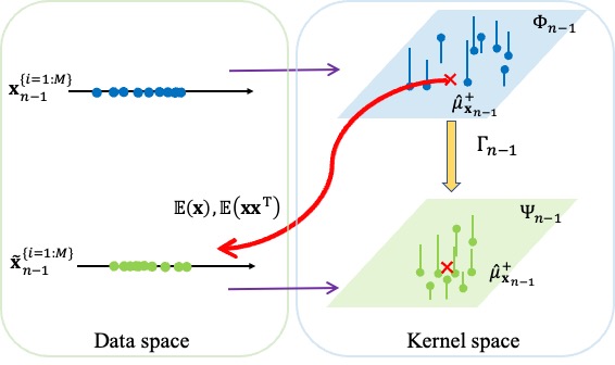
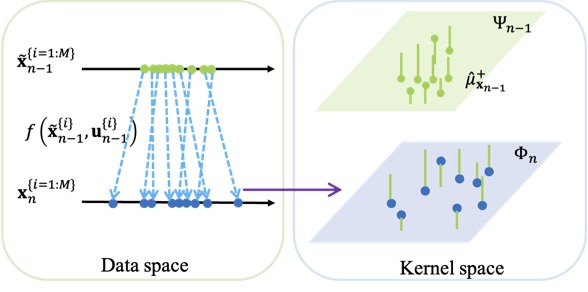
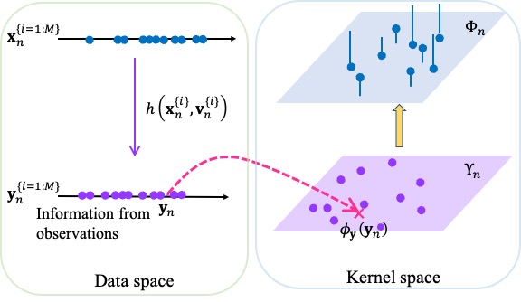
Figure 1: One iteration of the AKKF. Here, $M$ represents the number of particles. (a) Proposal step: embedding the posterior distribution at time $n-1$. Draw the proposal particles $\uline{\mathbf{x}}_{n-1}^{\{i=1:M\}}$ in the data space according to the importance distribution accessed from $\hat{\mu}_{\mathbf{x}_{n-1}}^{+}$. Then, the proposal kernel weight mean vector and covariance matrix are updated in the kernel space. (b) Prediction step: the particles are propagated through process function in the data space. Then the KME of the predictive distribution is approximated as $p(\mathbf{x}_{n}|\mathbf{x}_{1:n-1},\mathbf{y}_{1:n-1})\rightarrow\hat{\mu}_{\mathbf{x}_{n}}^{-}$. (c) Update step: the information from the new observation is used to update the kernel weight mean vector and covariance matrix. The KME of the posterior pdf $p(\mathbf{x}_{n}|\mathbf{x}_{1:n-1},\mathbf{y}_{1:n})\rightarrow\hat{\mu}_{\mathbf{x}_{n}}^{+}$ is calculated based on the observation information.

The rest of the paper is set out as follows. Section II reviews the KME [21] and the KKR [23]. Section III is devoted to the theoretical derivation of the proposed AKKF. In Section IV, we use three typical examples to present the performance results of the AKKF for non-linear problems and finally draw conclusions in Section V.

List of Abbreviations:

AKKF	Adaptive kernel Kalman filter
BOT	Bearings-only tracking
CV	Constant-velocity
DSSM	Dynamic state-space model
EKF	Extended Kalman filter
GPF	Gaussian particle filter
KBR	Kernel Bayesian rule
KF	Kalman filter
KME	Kernel mean embedding
KKR	Kernel Kalman rule
LMSE	Logarithmic mean square error
ML	Maximum-likelihood
MSE	Mean square error
PF	Particle filter
RKHS	Reproducing kernel Hilbert space
UKF	Unscented Kalman filter
UNGM	Univariate nonstationary growth model

II Preliminaries

This section briefly reviews the framework of the KME, empirical KME, and data-driven KKR. See [21] and [23] for details.

II-A Kernel Mean Embedding

A random variable is denoted as $X$ in the data space $\mathcal{X}$ with a pdf $p(\mathbf{x})$. An instance of $X$ is denoted as $\mathbf{x}$. A reproducing kernel Hilbert space (RKHS) denoted as ${\cal H}_{\mathbf{x}}$ on the data space $\mathcal{X}$ with a kernel function ${k}_{\mathbf{x}}(\mathbf{x},\mathbf{x}^{\prime})$ is defined as a Hilbert space of functions $f(\cdot)$ with the inner product $\langle\cdot,\cdot\rangle_{{\cal H}_{\mathbf{x}}}$ that satisfies the following important properties:

• The feature mapping of $\mathbf{x}$: $\phi_{\mathbf{x}}(\mathbf{x})={k}_{\mathbf{x}}(\mathbf{x},\cdot)\in{\cal H}_{\mathbf{x}}$ for all $\mathbf{x}\in\mathcal{X}$.

• Reproducing property: $f(\mathbf{x})=\langle f,{k}_{\mathbf{x}}(\mathbf{x},·)\rangle_{{\cal H}_{\mathbf{x}}}$ for all $f\in{\cal H}_{\mathbf{x}}$ and $\mathbf{x}\in\mathcal{X}$.

The above definitions are also applied to the predecessor of current state ${X}$, i.e., $\uline{X}$, and the observation variable, i.e., $Y$, that sit in two RKHSs. See Table I for a summary. The kernel function is the inner product of two feature mappings, i.e., $\langle\phi_{\mathbf{x}}(\mathbf{x}),\phi_{\mathbf{x}}(\mathbf{x}^{\prime})\rangle_{{\cal H}_{\mathbf{x}}}={k}_{\mathbf{x}}(\mathbf{x},\mathbf{x}^{\prime})$. Table II gives some typical kernel functions assuming a scalar $\mathbf{x}$. This paper investigates both infinite-dimension and finite-dimension feature spaces in a common framework.

Table I: The meaning of notations.

Description	Current state	predecessor state	Observation
Random variable	$X$	$\underline{X}$	$Y$
Domain	$\mathcal{X}$	$\mathcal{X}$	$\mathcal{Y}$
Specific variable	$\mathbf{x}$	$\uline{\mathbf{x}}$	$\mathbf{y}$
Kernel	${k}_{\mathbf{x}}(\mathbf{x},\mathbf{x}^{\prime})$	${k}_{\mathbf{x}}(\uline{\mathbf{x}},\uline{\mathbf{x}}^{\prime})$	${k}_{\mathbf{y}}(\mathbf{y},\mathbf{y}^{\prime})$
Kernel matrix	$K_{\mathbf{x}\mathbf{x}}$	$K_{\uline{\mathbf{x}}\uline{\mathbf{x}}}$	$G_{\mathbf{y}\mathbf{y}}$
Feature mapping	$\phi_{\mathbf{x}}(\mathbf{x})$	$\phi_{\mathbf{x}}(\uline{\mathbf{x}})$	$\phi_{\mathbf{y}}(\mathbf{y})$
Feature matrix	$\Phi$	$\Psi$	$\Upsilon$
RKHS	${\cal H}_{\mathbf{x}}$	${\cal H}_{\mathbf{x}}$	${\cal H}_{\mathbf{y}}$

The KME approach represents a pdf $p(\mathbf{x})$ by an element in the RKHS as

$$\mu_{X}:=\mathbb{E}_{X}\left[\phi_{\mathbf{x}}(X)\right]=\int_{\mathcal{X}}\phi_{\mathbf{x}}(\mathbf{x})p(\mathbf{x})d\mathbf{x}.$$ (7)

The joint pdf of two or more variables, e.g., $p(\mathbf{x},\mathbf{y})$, can be embedded into a tensor product feature space ${\cal H}_{\mathbf{x}}\otimes{\cal H}_{\mathbf{y}}$ as a (uncentered) covariance operator, i.e.,

$$\mathcal{C}_{XY}: =\mathbb{E}_{XY}\left[\phi_{\mathbf{x}}(X)\otimes\phi_{\mathbf{y}}(Y)\right]$$ (8)

$$=\int_{\mathcal{X}\times\mathcal{Y}}\phi_{\mathbf{x}}(\mathbf{x})\otimes\phi_{\mathbf{y}}(\mathbf{y})p(\mathbf{x},\mathbf{y})d\mathbf{x}d\mathbf{y}.$$

The tensor product features satisfy $\langle\phi_{\mathbf{x}}(\mathbf{x})\otimes\phi_{\mathbf{y}}(\mathbf{y}),\phi_{\mathbf{x}}(\mathbf{x}^{\prime})\otimes\phi_{\mathbf{y}}(\mathbf{y}^{\prime})\rangle_{{\cal H}_{\mathbf{x}}\otimes{\cal H}_{\mathbf{y}}}={k}_{\mathbf{x}}(\mathbf{x},\mathbf{x}^{\prime}){k}_{\mathbf{y}}(\mathbf{y},\mathbf{y}^{\prime})$.

Similar to (7), the KME of a conditional pdf $p(X|\mathbf{y})$ can be defined as

$$\mu_{X|\mathbf{y}}:=\mathbb{E}_{X|\mathbf{y}}\left[\phi_{\mathbf{x}}(X)\right]=\int_{\mathcal{X}}\phi_{\mathbf{x}}(\mathbf{x})p(\mathbf{x}|\mathbf{y})d\mathbf{x}.$$ (9)

The difference between the KME $\mu_{X|\mathbf{y}}$ and $\mu_{X}$ is that $\mu_{X}$ is a single element in the RKHS, while $\mu_{X|\mathbf{y}}$ is a family of points, each indexed by fixing $Y$ to a particular value $\mathbf{y}$. A conditional operator $\mathcal{C}_{X|Y}$ is defined under certain conditions [22] as the linear operator, which takes the feature mapping of a fixed value $\mathbf{y}$ as the input and outputs the corresponding conditional KME;

$$\mu_{X|\mathbf{y}}=\mathcal{C}_{X|Y}\phi_{\mathbf{y}}(\mathbf{y})=\mathcal{C}_{XY}\mathcal{C}^{-1}_{YY}\phi_{\mathbf{y}}(\mathbf{y}).$$ (10)

In practice, it is difficult to make valid statistical inferences about the regression parameters with an ill-conditioned covariance operator. Therefore, the inversion of $\mathcal{C}_{YY}$ is generally replaced by the regularized inverse, i.e., $\left(\mathcal{C}_{YY}+{\kappa}I\right)^{-1}$, where $\kappa$ is a regularization parameter to ensure that the inverse is well-defined, and $I$ is the identity operator matrix. When the conditions defined in [22] are not precisely met, (10) can still be interpreted as a linear (in the feature space) minimum mean squared error estimate for $\mu_{X|y}$.

Table II: Typical kernel functions.

Kernel function	$k({\mathbf{x}},{\mathbf{x}^{\prime}})$	Dimension of feature mapping
Linear	$\langle{\mathbf{x}},{\mathbf{x}^{\prime}}\rangle$	Finite
Quadratic	$\left(\langle{\mathbf{x}},{\mathbf{x}^{\prime}}\rangle+c\right)^{2}$	Finite
Quartic	$\left(\langle{\mathbf{x}},{\mathbf{x}^{\prime}}\rangle+c\right)^{4}$	Finite
Gaussian	$\exp\left(-\frac{1}{\sigma^{2}}\|({\mathbf{x}}-{\mathbf{x}^{\prime}})\|^{2}\right)$	Infinite

II-B Empirical Estimation of KME

As it is rare to access the actual underlying pdfs mentioned above, we can alternatively estimate the KMEs using a finite number of samples drawn from the corresponding pdfs.

The empirical KME of $p(\mathbf{x})$ in (7) is approximated as the average of the samples’ feature mappings, i.e., $\mathcal{D}_{\phi_{\mathbf{x}}(X)}=\{\phi_{\mathbf{x}}(\mathbf{x}^{\{1\}}),\dots,\phi_{\mathbf{x}}(\mathbf{x}^{\{M\}})\}$, the samples $\mathcal{D}_{X}=\{\mathbf{x}^{\{1\}},\dots,\mathbf{x}^{\{M\}}\}$ are drawn i.i.d. from $p(\mathbf{x})$, and $M$ represents the number of samples;

$$\hat{\mu}_{X}=\frac{1}{M}\sum_{i=1}^{M}\phi_{\mathbf{x}}(\mathbf{x}^{\{i\}}).$$ (11)

The empirical KME of the covariance operator $\mathcal{C}_{XY}$ in (8) inherits the injectivity of $\mathcal{C}_{XY}$ and is approximated as

$$\hat{\mathcal{C}}_{XY}=\frac{1}{M}\sum_{i=1}^{M}\phi_{\mathbf{x}}(\mathbf{x}^{\{i\}})\otimes\phi_{\mathbf{y}}(\mathbf{y}^{\{i\}})=\frac{1}{M}\Phi\Upsilon^{\rm{T}},$$ (12)

where the $M$ sample pairs $\mathcal{D}_{XY}=\{(\mathbf{x}^{\{1\}},\mathbf{y}^{\{1\}}),\dots,(\mathbf{x}^{\{M\}},\mathbf{y}^{\{M\}})\}$ are drawn i.i.d. from $p(\mathbf{x},\mathbf{y})$ with the feature mappings $\Phi:=\left[\phi_{\mathbf{x}}(\mathbf{x}^{\{1\}}),\dots,\phi_{\mathbf{x}}(\mathbf{x}^{\{M\}})\right]$ and $\Upsilon:=\left[\phi_{\mathbf{y}}(\mathbf{y}^{\{1\}}),\dots,\phi_{\mathbf{y}}(\mathbf{y}^{\{M\}})\right]$.

The KME of the conditional distribution $p(\mathbf{x}|\mathbf{y})$ is theoretically calculated as (9) or (10). When $p(\mathbf{x}|\mathbf{y})$ is unknown but i.i.d. samples $\mathcal{D}_{XY}$ drawn from $p(\mathbf{x},\mathbf{y})$ are available, the estimation of the empirical conditional operator $\hat{\mathcal{C}}_{X|Y}$ is regarded as a linear regression in the RKHS [24, 25]. And $\hat{\mathcal{C}}_{X|Y}$ is calculated by

$$\begin{split}\hat{\mathcal{C}}_{X|Y}=\hat{\mathcal{C}}_{XY}\left(\hat{\mathcal{C}}_{YY}+\kappa I\right)^{-1}=\Phi\left(G_{\mathbf{y}\mathbf{y}}+\kappa I\right)^{-1}\Upsilon^{\rm{T}}.\end{split}$$ (13)

Here, $G_{\mathbf{y}\mathbf{y}}=\Upsilon^{\rm{T}}\Upsilon$ is the Gram matrix for the samples from the observed variable $Y$. Then, the empirical KME of the conditional distribution is calculated through the following linear algebra as

$$\hat{\mu}_{X|\mathbf{y}}=\hat{\mathcal{C}}_{X|Y}\phi(\mathbf{y})=\Phi\left(G_{\mathbf{y}\mathbf{y}}+\kappa I\right)^{-1}\Upsilon^{\rm{T}}\phi_{\mathbf{y}}(\mathbf{y}){\equiv}\Phi\mathbf{w}.$$ (14)

Here, $\mathbf{y}\in\mathcal{Y}$ is the input test variable. Note that the empirical KME of the conditional pdf $\hat{\mu}_{X|\mathbf{y}}$ is a weighted sum of the feature mappings of the training samples. The weight vector includes $M$ non-uniform weights, i.e., ${\mathbf{w}}=\left[w^{\{1\}},\dots,w^{\{M\}}\right]^{\rm{T}}$, and is calculated as

$$\mathbf{w}=\left(G_{\mathbf{y}\mathbf{y}}+\kappa I\right)^{-1}G_{:,\mathbf{y}},$$ (15)

where the vector of kernel functions $G_{:,\mathbf{y}}=\left[{k}_{\mathbf{y}}(\mathbf{y}^{\{1\}},\mathbf{y}),\dots,{k}_{\mathbf{y}}(\mathbf{y}^{\{M\}},\mathbf{y})\right]^{\rm{T}}$. From (15), we can see that the kernel weight vector is the solution to a set of linear equations in the feature space, and unlike PF methods there are no non-negativity or normalization constraints.

II-C Kernel Kalman Rule

Based on the KME of conditional pdfs, non-linear estimations can be mapped into kernel feature spaces, i.e., RKHSs, and solved using linear operations. It has been proposed that the conditional KME operator in (10) can then be used to derive a KBR under certain conditions [21, 22]. However, these conditions are very restrictive and often fail, making the formulation difficult to interpret theoretically and quite unstable practically. Recently an alternative, the kernel Kalman rule (KKR) has been proposed exploiting the optimal linear interpretation (in the kernel feature space) of the conditional KME estimate that enjoys better stability [23].

The empirical KKR is formulated by executing a KF in the kernel feature space. An illustration of the KKR is shown in Fig. 2. Specifically, the transition matrix and the transition residual are calculated based on the training data set that is assumed to include $M$ sample triples $\mathcal{D}_{\uline{X}XY}=\{(\uline{\mathbf{x}}^{\{1\}},\mathbf{x}^{\{1\}},\mathbf{y}^{\{1\}}),\dots,(\uline{\mathbf{x}}^{\{M\}},\mathbf{x}^{\{M\}},\mathbf{y}^{\{M\}})\}$ [23]. Here, $\uline{\mathbf{x}}^{\{i\}}$ denotes the predecessor state of ${\mathbf{x}}^{\{i\}},i=1,\dots,M$, and $\mathbf{y}^{\{i\}}$ is the corresponding observation of ${\mathbf{x}}^{\{i\}}$. The feature mappings of the training data are represented as $\uline{\Phi}:=\left[\phi_{\mathbf{x}}(\uline{\mathbf{x}}^{\{1\}})\dots,\phi_{\mathbf{x}}(\uline{\mathbf{x}}^{\{M\}})\right]$, ${\Phi}:=\left[\phi_{\mathbf{x}}({\mathbf{x}}^{\{1\}})\dots,\phi_{\mathbf{x}}({\mathbf{x}}^{\{M\}})\right]$ and ${\Upsilon}:=\left[\phi_{\mathbf{y}}(\mathbf{y}^{\{1\}})\dots,\phi_{\mathbf{y}}(\mathbf{y}^{\{M\}})\right]$, respectively. The corresponding kernel weight mean vector and its covariance matrix are calculated following the prediction and update steps in the weight space.

In the prediction step, the kernel weight vector and covariance matrix from time $n-1$ to time $n$ are predicted in the weight space as

$$\mathbf{w}^{-}_{n}=T\mathbf{w}^{+}_{n-1},$$ (16)

$$S^{-}_{n}=TS^{+}_{n-1}T^{\rm{T}}+V.$$ (17)

Here, the kernel transition matrix $T$ is calculated based on the training predecessor states and training states data as $T=\left(K_{\uline{\mathbf{x}}\uline{\mathbf{x}}}+{{\lambda}_{\uline{K}}}I\right)^{-1}K_{\uline{\mathbf{x}}\mathbf{x}}$, and $V$ represents the transition residual [27]. ${K}_{\uline{\mathbf{x}}\mathbf{x}}=\uline{\Phi}^{\rm{T}}\Phi$ is the transition Gram matrix, and ${K}_{\uline{\mathbf{x}}\uline{\mathbf{x}}}=\uline{\Phi}^{\rm{T}}\uline{\Phi}$ is the Gram matrix of the predecessor states, ${\lambda}_{\uline{K}}$ is the regularization parameter to stabilize the inverse of ${K}_{\uline{\mathbf{x}}\uline{\mathbf{x}}}$. The predictive KME and covariance operator estimates are then calculated as $\mu_{\mathbf{x}_{n}}^{-}=\Phi\mathbf{w}^{-}_{n}$ and $\mathcal{C}_{\mathbf{x}_{n}\mathbf{x}_{n}}^{-}=\Phi S^{-}_{n}\Phi^{\rm{T}}$, respectively.

Next, the innovation update is executed based the kernel Kalman gain $Q_{n}$ calculation in the update step, i.e.,

$$\mathbf{w}^{+}_{n}=\mathbf{w}^{-}_{n}+Q_{n}\left({G_{:,\mathbf{y}_{n}}}-G_{\mathbf{y}\mathbf{y}}\mathbf{w}^{-}_{n}\right),$$ (18)

$$S^{+}_{n}=S^{-}_{n}-Q_{n}G_{\mathbf{y}\mathbf{y}}S^{-}_{n},$$ (19)

$$Q_{n}=S^{-}_{n}\left(G_{\mathbf{y}\mathbf{y}}S^{-}_{n}+\kappa I\right)^{-1},$$ (20)

where the Gram matrix of the training observations is $G_{\mathbf{y}\mathbf{y}}=\Upsilon^{\rm{T}}\Upsilon$. The test observation at time $n$ is $\mathbf{y}_{n}$, the kernel function vector between the training observations and the test observation is $G_{:,\mathbf{y}_{n}}=\left[{k}_{\mathbf{y}}(\mathbf{y}^{\{1\}},\mathbf{y}_{n}),\dots,{k}_{\mathbf{y}}(\mathbf{y}^{\{M\}},\mathbf{y}_{n})\right]^{\rm{T}}$. The updated KME and covariance operator estimates are then calculated as $\mu_{\mathbf{x}_{n}}^{+}=\Phi\mathbf{w}^{+}_{n}$ and $\mathcal{C}_{\mathbf{x}_{n}\mathbf{x}_{n}}^{+}=\Phi S^{+}_{n}\Phi^{\rm{T}}$, respectively. If the KME contains linear functions, e.g., when quadratic or quartics kernels are used, we can directly calculate the mean and covariance of the hidden states in the data space as marginal quantities of the estimated KME. Even when this is not possible, e.g., as with Gaussian kernels, a good approximation can be obtained by projecting the estimated KME into the data space as (21) and (22) [27] where it is implicitly assumed that functions in kernel feature spaces can reasonably approximate the linear and quadratic functions;

$$\hat{\mathbf{x}}_{n}=X_{\mathcal{D}}\mathbf{w}^{+}_{n},$$ (21)

$$\hat{\Sigma}_{n}=X_{\mathcal{D}}S^{+}_{n}X_{\mathcal{D}}^{\rm{T}},$$ (22)

where $X_{\mathcal{D}}=\left[\mathbf{x}^{\{1\}},\dots,\mathbf{x}^{\{M\}}\right]$ is the set of the current training states.

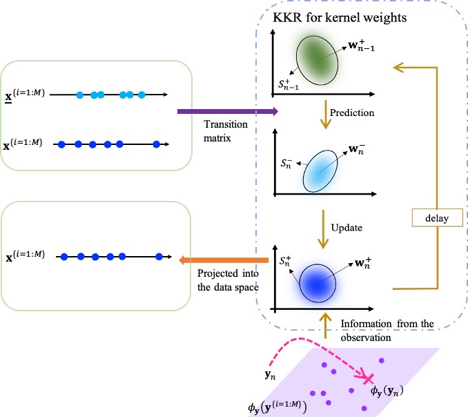
Figure 2: One iteration of the KKR. Here, $\uline{\mathbf{x}}^{\{i=1:M\}}$, $\mathbf{x}^{\{i=1:M\}}$, and $\mathbf{y}^{\{i=1:M\}}$ denotes the deterministic training predecessor hidden states, current hidden states, and observations, respectively. The kernel weight mean vector and covariance matrix are predicted and updated as a KF in kernel spaces. The estimations of hidden states are found by projecting the kernel weights into the training data space. 1. Prediction step: The predictive kernel weight vector and matrix are updated based on the transition matrix $T$. 2. Update step: The posterior kernel weight vector and matrix are updated according to the information of the new observation $\mathbf{y}_{n}$.

The kernel-based filters learn the probabilistic transition and observation dynamics as linear functions on embeddings of the belief state in high-dimensional RKHSs from training data. Note that existing filters based on the KME or the KKR are entirely data-driven, requiring the training data to provide sufficient statistics of the dynamic systems and, therefore, of use when the DSSM is unavailable. The tracking applications of the KKR so far include table tennis balls track, human motion activity estimation, and pendulum track [23]. These applications all have the weakness that the high-dimensional RKHSs are limited with the training data, which requires high similarities between the test data and the training data. However, the entirely data-driven filter’s tracking performance is vulnerable and will fail catastrophically when the target moves out of the training space. This is particularly a problem in the case for the real-time tracking applications that we focus on here. To the best of our knowledge, other investigations have not considered the issue of incorporating a DSSM into the RKHS setting.

Unlike the KKR, this paper proposes a Bayesian filter called the adaptive kernel Kalman filter (AKKF) that provides a mechanism for applying the data-driven kernel method to model-based systems. Specifically, there is no need for any training data or an offline training process of the AKKF. The AKKF adaptively draws new particles whose weighted features match the current KME estimate. These particles can then be precisely propagated through the non-linearity and used to calculate empirical transition operators in the RKHS on the fly. The embeddings of updated state particles can be seen as providing an adaptive change of basis for the high-dimensional RKHSs, making the non-linear function approximation more accurate and flexible. Therefore, the AKKF has higher efficiency and broader applications.

III Adaptive Kernel Kalman Filter

The proposed AKKF aims to take all the benefits of the KME and KKR, and adapt them to work in the model-based setup. I.e., the presented AKKF is a method incorporating a DSSM into RKHSs. In a similar manner to the selection and propagation of sigma points in the UKF, the AKKF adaptively updates particles whose weighted features are matched to the KME estimate of the current state. Note that the AKKF chooses particles propagated through the non-linear system randomly, which is different from the UKF. Further, the weights of the proposed AKKF, unlike PFs, do not need to be normalized or non-negative and are updated through simple linear regression.

In the proposed AKKF, the empirical KME of the hidden state’s posterior pdf requires a set of generated particles’ feature mappings and the corresponding kernel weights. Fig. 1 shows one iteration of the proposed AKKF executed in both the data and kernel feature spaces. Specifically, particles are updated and propagated in the data space based on parametric DSSMs to capture the diversity of the non-linearities. The corresponding kernel weight mean vector and covariance matrix are predicted and updated by matching (or approximating in a least squares manner in the feature space) with the state KME. The following presents three main steps of the proposed AKKF.

III-A Embedding the Posterior Distribution at Time $n-1$

Given the posterior KME estimate at time $n-1$, i.e., $\hat{\mu}^{+}_{\mathbf{x}_{n-1}}$, we wish to draw new particles that better represent the probability mass of the associated posterior pdf. The posterior KME estimate $\hat{\mu}^{+}_{\mathbf{x}_{n-1}}$ comprises weighted feature mappings of the particles, for which we use blue points to represent in Fig. 1. While there are sophisticated iterative methods, such as herding [28], that can sample from the posterior distribution. We advocate a much simpler technique in the spirit of importance sampling. Given that we can extract estimates for the mean and covariance of the state pdf in data space, we can draw particles in the high probability region of the pdf by sampling from a Gaussian distribution with matched mean and covariance. These particles can then be used to generate a new approximation of the KME of the pdf through appropriate reweighting.

Specifically, the particles and the corresponding kernel feature mappings at time slot $n-1$ are represented as $\mathbf{x}^{\{i=1:M\}}_{n-1}$ and $\phi_{\mathbf{x}}(\mathbf{x}^{\{i=1:M\}}_{n-1})$, respectively. And the empirical KME and the covariance operator of $p(\mathbf{x}_{n-1}\mid\mathbf{x}_{0:n-1},\mathbf{y}_{1:n-1})$ were calculated as

$$\hat{\mu}^{+}_{\mathbf{x}_{n-1}} =\Phi_{n-1}\mathbf{w}^{+}_{n-1},$$ (23)

$$\hat{\mathcal{C}}_{\mathbf{x}_{n},\mathbf{x}_{n}} =\Phi_{n}S_{n}^{+}\Phi_{n}^{\rm{T}},$$ (24)

where $\Phi_{n-1}=\left[\phi_{\mathbf{x}}(\mathbf{x}_{n-1}^{\{1\}}),\dots,\phi_{\mathbf{x}}(\mathbf{x}_{n-1}^{\{M\}})\right]$. Then, the state mean and covariance (in data space) of $\mathbf{x}_{n-1}$, i.e., $\mathbb{E}(\mathbf{x}_{n-1})$ and $\mathrm{Cov}(\mathbf{x}_{n-1})$, are extracted from $\hat{\mu}^{+}_{\mathbf{x}_{n-1}}$ and returned to the data space, as shown by the red arrow in Fig. 1.

The state vector’s mean and covariance are extracted in two different ways: 1) A suitable kernel choice, i.e., quadratic and quartic kernels, can directly give the state vector’s mean and covariance if the associated RKHS contains linear functions. For example, suppose $\mathbf{x}_{n-1}=\left[{x}_{n-1,1},\dots,{x}_{n-1,d}\right]^{\rm{T}}$ is a $d$-dimension vector, with the utilization of quadratic kernel, the empirical KME $\hat{\mu}_{\mathbf{x}_{n-1}}^{+}$ is represented as (25) which contains all features of degree zero, degree one, and degree two terms;

$$\hat{\mu}_{\mathbf{x}_{n-1}}^{+}=\left[\mathrm{vec}\left(\mathbb{E}{\left(\mathbf{x}_{n-1}\mathbf{x}_{n-1}^{\rm{T}}\right)}\right)^{\rm{T}},\left(\mathbb{E}{\left(\mathbf{x}_{n-1}\right)}\right)^{\rm{T}},c\right]^{\rm{T}}.$$ (25)

Here, $c\geq 0$ is a free parameter trading off the influence from higher-order and lower-order terms of the polynomial [29]. The utilization of quartic kernel can further provide all features of degree zero to degree four terms; 2) Otherwise, such as linear or Gaussian kernels, the state vector’s mean and covariance can be approximated using (21) and (22). Then, the proposal particles, shown as green points in Fig. 1 can be randomly sampled from the following normal distribution as

$$\tilde{\mathbf{x}}_{n-1}^{\{i=1:M\}} \sim\mathcal{N}\left(\mathbb{E}\left(\mathbf{x}_{n-1}\right),\mathrm{Cov}\left(\mathbf{x}_{n-1}\right)\right),$$ (26)

$$\mathrm{Cov}\left(\mathbf{x}_{n-1}\right) =\mathbb{E}\left(\mathbf{x}_{n-1}\mathbf{x}_{n-1}^{\rm{T}}\right)-\mathbb{E}\left(\mathbf{x}_{n-1}\right)\mathbb{E}\left(\mathbf{x}_{n-1}\right)^{\rm{T}}.$$ (27)

For convenience, we draw the proposal particles from a Gaussian distribution, although other distributions with matched statistics could also conceivably be used. The proposal particles should therefore capture the location of the significant probability mass of the posterior pdf. In order to use these particles to approximate the KME of the posterior pdf, we need to calculate new kernel weights for them, i.e, $\tilde{\mathbf{w}}^{+}_{n-1}$. Note that this is not equivalent to approximating the posterior pdf by a Gaussian. Instead, it can be thought of as an adaptive change of basis within the feature space which can be achieved through a simple linear mapping that we describe next. Let the proposal particles’ feature mappings be represented as $\Psi_{n-1}=\left[\phi_{\mathbf{x}}(\tilde{\mathbf{x}}_{n-1}^{\{1\}}),\dots,\phi_{\mathbf{x}}(\tilde{\mathbf{x}}_{n-1}^{\{M\}})\right]$, with the associated weight vector $\tilde{\mathbf{w}}^{+}_{n-1}$ and matrix $\tilde{S}^{+}_{n-1}$. Then, the KME and covariance operator in (23) and (24) are rewritten as

$$\hat{\mu}^{+}_{\mathbf{x}_{n-1}} =\Psi_{n-1}\tilde{\mathbf{w}}^{+}_{n-1},$$ (28)

$$\hat{\mathcal{C}}^{+}_{\mathbf{x}_{n-1}\mathbf{x}_{n-1}} =\Psi_{n-1}\tilde{{S}}^{+}_{n-1}\Psi_{n-1}^{\mathrm{T}}.$$ (29)

The formulas for the proposal kernel weight vector $\tilde{\mathbf{w}}^{+}_{n-1}$ and matrix $\tilde{S}^{+}_{n-1}$ are (30) and (31), respectively.

$$\Psi_{n-1}\tilde{\mathbf{w}}^{+}_{n-1}=\Phi_{n-1}\mathbf{w}^{+}_{n-1}$$ (30)

$$\Rightarrow \Psi_{n-1}^{\mathrm{T}}\Psi_{n-1}\tilde{\mathbf{w}}^{+}_{n-1}=\Psi_{n-1}^{\mathrm{T}}\Phi_{n-1}\mathbf{w}^{+}_{n-1}$$

$$\Rightarrow \tilde{\mathbf{w}}^{+}_{n-1}=\left(\Psi_{n-1}^{\mathrm{T}}\Psi_{n-1}\right)^{-1}\Psi_{n-1}^{\mathrm{T}}\Phi_{n-1}\mathbf{w}^{+}_{n-1}$$

$$\Rightarrow \tilde{\mathbf{w}}^{+}_{n-1}=\left(K_{\tilde{\mathbf{x}}\tilde{\mathbf{x}}}+{\lambda_{\tilde{K}}}I\right)^{-1}K_{\tilde{\mathbf{x}}\mathbf{x}}\mathbf{w}^{+}_{n-1}=\Gamma_{n-1}\mathbf{w}^{+}_{n-1},$$

$$\Psi_{n-1}\tilde{{S}}^{+}_{n-1}\Psi_{n-1}^{\mathrm{T}}=\Phi_{n-1}{S}^{+}_{n-1}\Phi_{n-1}^{\mathrm{T}}$$ (31)

$$\Rightarrow \Psi_{n-1}^{\mathrm{T}}\Psi_{n-1}\tilde{{S}}^{+}_{n-1}\Psi_{n-1}^{\mathrm{T}}\Psi_{n-1}=\Psi_{n-1}^{\mathrm{T}}\Phi_{n-1}{S}^{+}_{n-1}\Phi_{n-1}^{\mathrm{T}}\Psi_{n-1}$$

$$\Rightarrow \tilde{S}^{+}_{n-1}=\left[\left(K_{\tilde{\mathbf{x}}\tilde{\mathbf{x}}}+{\lambda_{\tilde{K}}}I\right)^{-1}K_{\tilde{\mathbf{x}}\mathbf{x}}\right]{S}^{+}_{n-1}\left[\left(K_{\tilde{\mathbf{x}}\tilde{\mathbf{x}}}+{\lambda_{\tilde{K}}}I\right)^{-1}K_{\tilde{\mathbf{x}}\mathbf{x}}\right]^{\mathrm{T}}$$

$$\Rightarrow \tilde{S}^{+}_{n-1}=\Gamma_{n-1}{S}^{+}_{n-1}\Gamma_{n-1}^{\mathrm{T}}.$$

Here, $\Gamma_{n-1}$ represents the change of sample representation from $\Phi_{n-1}$ to $\Psi_{n-1}$ and is calculated as $\Gamma_{n-1}=\left(K_{\tilde{\mathbf{x}}\tilde{\mathbf{x}}}+{\lambda_{\tilde{K}}}I\right)^{-1}K_{\tilde{\mathbf{x}}\mathbf{x}}$. The matrix $K_{\tilde{\mathbf{x}}\tilde{\mathbf{x}}}=\Psi^{\rm{T}}_{n-1}\Psi_{n-1}$ represents the Gram matrix of the proposal particles at time $n-1$. The matrix $K_{\tilde{\mathbf{x}}\mathbf{x}}=\Psi^{\rm{T}}_{n-1}\Phi_{n-1}$ represents the Gram matrix between the old particles $\mathbf{x}^{\{i=1:M\}}_{n-1}$ and the proposal particles $\tilde{\mathbf{x}}^{\{i=1:M\}}_{n-1}$ at time $n-1$. The regularization parameter $\lambda_{\tilde{K}}$ is used to stabilize the inverse of $K_{\tilde{\mathbf{x}}\tilde{\mathbf{x}}}$. Note that for small feature spaces, i.e., $\Phi$ is full rank, and $\mathrm{Dim}\left[\Phi\right]<M$, (28) and (29) are exact. However, to deal with ill-conditioning or where the feature space is larger than the number of samples, e.g., when it is infinite, using the weight vector and covariance matrix from (30) and (31) make (28) and (29) approximate.

III-B Prediction from Time $n-1$ to Time $n$

In this step, the proposal particles generated in the previous step are propagated through the process model to estimate the transition operator ${\mathcal{C}}_{\mathbf{x}_{n}|\mathbf{x}_{n-1}}$. Then the predictive kernel weight vector and covariance matrix are calculated.

Specifically, the proposal particles at time $n-1$ are propagated through the transition function to calculate the particles at time $n$, represented as indigo points in Fig. 1.

$$\mathbf{x}_{n}^{\{i\}}=f(\tilde{\mathbf{x}}_{n-1}^{\{i\}},\mathbf{u}_{n}^{\{i\}}),\quad i=1\dots M,$$ (32)

where $\mathbf{u}_{n}^{\{i\}}$ represents a process noise sample drawn from the process noise pdf. The feature mappings of $\mathbf{x}_{n}^{\{1:M\}}$ are $\Phi_{n}=\left[\phi_{\mathbf{x}}(\mathbf{x}_{n}^{\{1\}}),\dots,\phi_{\mathbf{x}}(\mathbf{x}_{n}^{\{M\}})\right]$, and the predictive KME and covariance operator are calculated by

$$\hat{\mu}^{-}_{\mathbf{x}_{n}}=\Phi_{n}\mathbf{w}^{-}_{n},$$ (33)

$$\hat{\mathcal{C}}^{-}_{\mathbf{x}_{n}\mathbf{x}_{n}}=\Phi_{n}\mathbf{S}^{-}_{n}\Phi_{n}^{\mathrm{T}}.$$ (34)

Here, the weight vector $\mathbf{w}^{-}_{n}$ and matrix $\mathbf{S}^{-}_{n}$ are derived in (35)–(41) as follows. The conditional KME of the transitional probability $p(\mathbf{x}_{n}|\mathbf{x}_{n-1},\mathbf{y}_{1:n-1})$ is approximated as

$$p(\mathbf{x}_{n}|\mathbf{x}_{n-1},\mathbf{y}_{1:n-1}) \mapsto\hat{\mu}_{\mathbf{x}_{n}}^{-}=\hat{\mathcal{C}}_{\mathbf{x}_{n}|\mathbf{x}_{n-1}}\hat{\mu}_{\mathbf{x}_{n-1}}^{+},$$ (35)

where the empirical approximations to the conditional embedding operator $\hat{\mathcal{C}}_{\mathbf{x}_{n}|\mathbf{x}_{n-1}}$ can be derived from a least-squares objective [30] as

$$\begin{split}\hat{\mathcal{C}}_{\mathbf{x}_{n}|\tilde{\mathbf{x}}_{n-1}}&=\Phi_{n}\left(\Psi_{n-1}\Psi^{\rm{T}}_{n-1}+\lambda_{\tilde{K}}I\right)^{-1}\Psi^{\rm{T}}_{n-1}\\ &=\Phi_{n}\left(K_{\tilde{\mathbf{x}}\tilde{\mathbf{x}}}+\lambda_{\tilde{K}}I\right)^{-1}\Psi^{\rm{T}}_{n-1}.\end{split}$$ (36)

Substituting (28) and (36) into (35), we have the estimate of the predictive empirical KME of $\mathbf{x}_{n}$ as

$$\begin{split}&\hat{\mu}_{\mathbf{x}_{n}}^{-}=\hat{\mathcal{C}}_{\mathbf{x}_{n}|\tilde{\mathbf{x}}_{n-1}}\hat{\mu}_{\mathbf{x}_{n-1}}^{+}\\ &=\Phi_{n}\left(K_{\tilde{\mathbf{x}}\tilde{\mathbf{x}}}+{\lambda_{\tilde{K}}}I\right)^{-1}\Psi^{\rm{T}}_{n-1}\Phi_{n-1}\mathbf{w}_{n-1}^{+}\\ &=\Phi_{n}\left(K_{\tilde{\mathbf{x}}\tilde{\mathbf{x}}}+{\lambda_{\tilde{K}}}I\right)^{-1}K_{\tilde{\mathbf{x}}\mathbf{x}}\mathbf{w}_{n-1}^{+}\\ &=\Phi_{n}\mathbf{w}_{n}^{-}.\end{split}$$ (37)

Thus, the estimate of the predictive kernel weight vector is given by

$$\mathbf{w}^{-}_{n}=\left(K_{\tilde{\mathbf{x}}\tilde{\mathbf{x}}}+{\lambda_{\tilde{K}}}I\right)^{-1}K_{\tilde{\mathbf{x}}\mathbf{x}}\mathbf{w}_{n-1}^{+}=\Gamma_{n-1}\mathbf{w}^{+}_{n-1}.$$ (38)

From (30) and (38), we see that $\mathbf{w}^{-}_{n}=\tilde{\mathbf{w}}^{+}_{n-1}$. Next, the empirical predictive covariance operator at time $n$ is computed as

$$\hat{\mathcal{C}}_{\mathbf{x}_{n}\mathbf{x}_{n}}^{-} =\hat{\mathcal{C}}_{\mathbf{x}_{n}|\tilde{\mathbf{x}}_{n-1}}\hat{\mathcal{C}}_{\mathbf{x}_{n-1}\mathbf{x}_{n-1}}^{+}\hat{\mathcal{C}}_{\mathbf{x}_{n}|\tilde{\mathbf{x}}_{n-1}}^{\mathrm{T}}+\mathcal{V}_{n}$$ (39)

$$=\hat{\mathcal{C}}_{\mathbf{x}_{n}|\tilde{\mathbf{x}}_{n-1}}\Psi_{n-1}\tilde{S}_{n-1}^{+}\Psi_{n-1}^{\mathrm{T}}\hat{\mathcal{C}}_{\mathbf{x}_{n}|\tilde{\mathbf{x}}_{n-1}}^{\mathrm{T}}+\mathcal{V}_{n}$$

$$=\Phi_{n}\tilde{S}_{n-1}^{+}\Phi_{n}^{\mathrm{T}}+\mathcal{V}_{n}.$$

Here, $\mathcal{V}_{n}$ represents the transition residual matrix, which is derived as

$$\mathcal{V}_{n} =\frac{1}{M}\left(\hat{\mathcal{C}}_{\mathbf{x}_{n}|\tilde{\mathbf{x}}_{n-1}}\Psi_{n-1}-\Phi_{n}\right)\left(\hat{\mathcal{C}}_{\mathbf{x}_{n}|\tilde{\mathbf{x}}_{n-1}}\Psi_{n-1}-\Phi_{n}\right)^{\mathrm{T}}$$ (40)

$$= \frac{1}{M}\left[\Phi_{n}\left(K_{\tilde{\mathbf{x}}\tilde{\mathbf{x}}}+\lambda_{\tilde{K}}I\right)^{-1}\Psi_{n-1}^{\mathrm{T}}\Psi_{n-1}-\Phi_{n}\right]$$

$$\times\left[\Phi_{n}\left(K_{\tilde{\mathbf{x}}\tilde{\mathbf{x}}}+\lambda_{\tilde{K}}I\right)^{-1}\Psi_{n-1}^{\mathrm{T}}\Psi_{n-1}-\Phi_{n}\right]^{\mathrm{T}}$$

$$= \Phi_{n}\frac{1}{M}\left[\left(K_{\tilde{\mathbf{x}}\tilde{\mathbf{x}}}+\lambda_{\tilde{K}}I\right)^{-1}K_{\tilde{\mathbf{x}}\tilde{\mathbf{x}}}-I\right]$$

$$\times\left[\left(K_{\tilde{\mathbf{x}}\tilde{\mathbf{x}}}+\lambda_{\tilde{K}}I\right)^{-1}K_{\tilde{\mathbf{x}}\tilde{\mathbf{x}}}-I\right]^{\mathrm{T}}\Phi_{n}^{\mathrm{T}}$$

$$\equiv \Phi_{n}V_{n}\Phi_{n}^{\mathrm{T}}.$$

Here, $V_{n}$ is the finite matrix representation of $\mathcal{V}_{n}$. The predictive weight covariance matrix is given by substituting (39) and (40) into (34);

$${S}_{n}^{-}=\tilde{S}_{n-1}^{+}+V_{n}.$$ (41)

III-C Update at Time $n$

This step modifies the predictive kernel weight vector and covariance matrix calculated in the previous step, considering the new observation at time $n$. The observation particles in Fig. 1 are updated based on the measurement model as

$$\mathbf{y}_{n}^{\{i\}}=h({\mathbf{x}}_{n}^{\{i\}},\mathbf{v}_{n}^{\{i\}}),\quad i=1\dots M.$$ (42)

Here, $\mathbf{v}_{n}^{\{i\}}$ represents a measurement noise sample drawn from the measurement noise pdf. Then, the kernel mappings of observation particles in the kernel feature space are $\Upsilon_{n}=\left[\phi_{\mathbf{y}}(\mathbf{y}_{n}^{\{1\}}),\dots,\phi_{\mathbf{y}}(\mathbf{y}_{n}^{\{M\}})\right]$. The posterior KME is calculated as

$$\hat{\mu}_{\mathbf{x}_{n}}^{+}=\hat{\mu}_{\mathbf{x}_{n}}^{-}+\mathcal{Q}_{n}\left[\phi_{\mathbf{y}}(\mathbf{y}_{n})-\hat{\mathcal{C}}_{\mathbf{y}_{n}|\mathbf{x}_{n}}\hat{\mu}_{\mathbf{x}_{n}}^{-}\right],$$ (43)

where the kernel Kalman gain operator denoted as $\mathcal{Q}_{n}$ is applied to the correction term $\phi_{\mathbf{y}}(\mathbf{y}_{n})-\hat{\mathcal{C}}_{\mathbf{y}_{n}|\mathbf{x}_{n}}\hat{\mu}_{\mathbf{x}_{n}}^{-}$ and is derived by minimizing the trace of the posterior covariance operator $\hat{\mathcal{C}}_{\mathbf{x}_{n}\mathbf{x}_{n}}^{+}$ [23], as in the (44):

$$\mathcal{Q}_{n} =\arg\min_{\mathcal{Q}_{n}}\mathrm{Tr}\left[{\hat{\mathcal{C}}_{\mathbf{x}_{n}\mathbf{x}_{n}}^{+}}\right]$$ (44)

$$=\Phi_{n}S_{n}^{-}\left(G_{\mathbf{y}\mathbf{y}}S_{n}^{-}+\kappa I\right)^{-1}\Upsilon_{n}^{\mathrm{T}}.$$

The Appendix provides the derivation details of $\mathcal{Q}_{n}$. Then, the updated KME vector represented in (43) is calculated as

$$\hat{\mu}_{\mathbf{x}_{n}}^{+}= \Phi_{n}{\mathbf{w}}^{+}_{n}=\Phi_{n}{\mathbf{w}}^{-}_{n}+\mathcal{Q}_{n}\left[\phi(\mathbf{y}_{n})-\hat{\mathcal{C}}_{\mathbf{y}_{n}|\mathbf{x}_{n}}\hat{\mu}_{\mathbf{x}_{n}}^{-}\right]$$ (45)

$$= \Phi_{n}\left[{\mathbf{w}}^{-}_{n}+S_{n}^{-}\left(G_{\mathbf{y}\mathbf{y}}S_{n}^{-}+\kappa I\right)^{-1}\left(G_{:,\mathbf{y}_{n}}-G_{\mathbf{y}\mathbf{y}}{\mathbf{w}}^{-}_{n}\right)\right],$$

where the kernel vector of the measurement at time $n$ is $G_{:,\mathbf{y}_{n}}=\Upsilon_{n}^{\mathrm{T}}\phi(\mathbf{y}_{n})$, and the Gram matrix of the observation at time $n$ is $G_{\mathbf{y}\mathbf{y}}=\Upsilon^{\mathrm{T}}_{n}\Upsilon_{n}$. Hence, the weight vector is updated as

$${\mathbf{w}}^{+}_{n} ={\mathbf{w}}^{-}_{n}+S_{n}^{-}\left(G_{\mathbf{y}\mathbf{y}}S_{n}^{-}+\kappa I\right)^{-1}\left(G_{:,\mathbf{y}_{n}}-G_{\mathbf{y}\mathbf{y}}{\mathbf{w}}^{-}_{n}\right)$$ (46)

$$={\mathbf{w}}^{-}_{n}+Q_{n}\left(G_{:,\mathbf{y}_{n}}-G_{\mathbf{y}\mathbf{y}}{\mathbf{w}}^{-}_{n}\right),$$

where $Q_{n}$ is the finite matrix representation of $\mathcal{Q}_{n}$;

$$Q_{n}=S_{n}^{-}\left(G_{\mathbf{y}\mathbf{y}}S_{n}^{-}+\kappa I\right)^{-1}.$$ (47)

Then, the covariance operator can be expressed as:

$$\hat{\mathcal{C}}_{\mathbf{x}_{n}\mathbf{x}_{n}}^{+}=\hat{\mathcal{C}}_{\mathbf{x}_{n}\mathbf{x}_{n}}^{-}-\mathcal{Q}_{n}\Upsilon_{n}S_{n}^{-}\Phi_{n}^{\mathrm{T}}.$$ (48)

The derivation details are shown in Appendix. As the predictive and posterior covariance operators are $\hat{\mathcal{C}}_{\mathbf{x}_{n}\mathbf{x}_{n}}^{-}=\Phi_{n}S_{n}^{-}\Phi_{n}^{\mathrm{T}}$ and $\hat{\mathcal{C}}_{\mathbf{x}_{n}\mathbf{x}_{n}}^{+}=\Phi_{n}S_{n}^{+}\Phi_{n}^{\mathrm{T}}$, (48) is rewritten as

$$\Phi_{n}S_{n}^{+}\Phi_{n}^{\mathrm{T}}=\Phi_{n}S_{n}^{-}\Phi_{n}^{\mathrm{T}}-\mathcal{Q}_{n}\Upsilon_{n}S_{n}^{-}\Phi_{n}^{\mathrm{T}}$$ (49)

$$\Rightarrow \Phi_{n}S_{n}^{+}\Phi_{n}^{\mathrm{T}}$$

$$=\Phi_{n}S_{n}^{-}\Phi_{n}^{\mathrm{T}}-\Phi_{n}S_{n}^{-}\Upsilon_{n}^{\mathrm{T}}\left(\Upsilon_{n}S_{n}^{-}\Upsilon_{n}^{\mathrm{T}}+\kappa I\right)^{-1}\Upsilon_{n}S_{n}^{-}\Phi_{n}^{\mathrm{T}}$$

$$=\Phi_{n}\left[S_{n}^{-}-S_{n}^{-}\Upsilon_{n}^{\mathrm{T}}\left(\Upsilon_{n}S_{n}^{-}\Upsilon_{n}^{\mathrm{T}}+\kappa I\right)^{-1}\Upsilon_{n}S_{n}^{-}\right]\Phi_{n}^{\mathrm{T}}.$$

Therefore, the kernel weight covariance matrix is finally updated as

$$S_{n}^{+} =S_{n}^{-}-S_{n}^{-}\Upsilon_{n}^{\mathrm{T}}\left(\Upsilon_{n}S_{n}^{-}\Upsilon_{n}^{\mathrm{T}}+\kappa I\right)^{-1}\Upsilon_{n}S_{n}^{-}$$ (50)

$$=S_{n}^{-}-S_{n}^{-}\left(G_{\mathbf{y}\mathbf{y}}S_{n}^{-}+\kappa I\right)^{-1}G_{\mathbf{y}\mathbf{y}}S_{n}^{-}$$

$$=S_{n}^{-}-Q_{n}G_{\mathbf{y}\mathbf{y}}S_{n}^{-}.$$

III-D Implementation of AKKF

Based on the above descriptions, Algorithm 1 summarizes the implementation of the AKKF.

Algorithm 1 Adaptive kernel Kalman filter

0:  DSSM: transition model $f(\cdot)$ and measurement model $h(\cdot)$.

1:  Initialization: Set the initial particles in real space $\mathbf{x}_{0}^{\{i=1:M\}}\sim P_{\text{init}}$, $\Phi_{0}:=\left[\phi_{\mathbf{x}}(\mathbf{x}_{0}^{\{1\}}),\dots,\phi_{\mathbf{x}}(\mathbf{x}_{0}^{\{M\}})\right]$, $\mathbf{w}_{0}=1/M\left[1,\dots,1\right]^{\rm{T}}$, $\Psi_{0}=\Phi_{0}$, $\Gamma_{0}=I$.

2:  for $n=1:N$ do

3:     Prediction:

• First, in the data space:

  $\mathbf{x}_{n}^{\{i\}}=f(\tilde{\mathbf{x}}_{n-1}^{\{i\}},\mathbf{u}_{n}^{\{i\}})$, $i=1\dots M$.

• Second, in the kernel feature space:

  $\Phi_{n}=\left[\phi_{\mathbf{x}}(\mathbf{x}_{n}^{\{1\}}),\dots,\phi_{\mathbf{x}}(\mathbf{x}_{n}^{\{M\}})\right]$,

  $\mathbf{w}^{-}_{n}=\tilde{\mathbf{w}}^{+}_{n-1}$,

  ${S}_{n}^{-}=\tilde{S}_{n-1}^{+}+V_{n}$.

4:     Update:

• First, in the data space:

  $\mathbf{y}_{n}^{\{i\}}=h(\mathbf{x}_{n}^{\{i\}},\mathbf{v}_{n}^{\{i\}})$, $i=1\dots M$.

• Second, in the kernel feature space:

  $\Upsilon_{n}=\left[\phi_{\mathbf{y}}(\mathbf{y}_{n}^{\{1\}}),\dots,\phi_{\mathbf{y}}(\mathbf{y}_{n}^{\{M\}})\right]$, $G_{\mathbf{y}\mathbf{y}}=\Upsilon_{n}^{\rm{T}}\Upsilon_{n}$.

  ${\mathbf{w}}^{+}_{n}={\mathbf{w}}^{-}_{n}+Q_{n}\left(G_{:,\mathbf{y}_{n}}-G_{\mathbf{y}\mathbf{y}}{\mathbf{w}}^{-}_{n}\right)$.

  $S_{n}^{+}=S_{n}^{-}-Q_{n}G_{\mathbf{y}\mathbf{y}}S_{n}^{-}.$

  The posterior KME with the statistical information:

  $\hat{\mu}_{\mathbf{x}_{n}}=\Phi_{n}\mathbf{w}^{+}_{n}=\left[\mathbb{E}{\left(\mathbf{x}_{n}\mathbf{x}_{n}^{\rm{T}}\right)},\mathbb{E}{\left(\mathbf{x}_{n}\right)},c\right]^{\rm{T}}$.

5:     Proposal particles draw:

• First, in the data space:

  $\tilde{\mathbf{x}}_{n}^{\{i=1:M\}}\sim\mathcal{N}\left(\mathbb{E}\left(\mathbf{x}_{n}\right),\mathbb{E}\left(\mathbf{x}_{n}\mathbf{x}_{n}^{\rm{T}}\right)-\mathbb{E}\left(\mathbf{x}_{n}\right)\mathbb{E}\left(\mathbf{x}_{n}\right)^{\rm{T}}\right)$.

• Second, in kernel feature space:

  $\Psi_{n}=\left[\phi_{\mathbf{x}}(\tilde{\mathbf{x}}_{n}^{\{1\}}),\dots,\phi_{\mathbf{x}}(\tilde{\mathbf{x}}_{n}^{\{M\}})\right]$.

  $\Gamma_{n}=\left(\Psi_{n}^{\rm{T}}\Psi_{n}+\lambda I\right)^{-1}{\Psi_{n}^{\rm{T}}\Phi_{n}}$.

  $\tilde{\mathbf{w}}^{+}_{n}=\Gamma_{n}\mathbf{w}^{+}_{n}$.

  $\tilde{\mathbf{S}}^{+}_{n}=\Gamma_{n}\mathbf{S}^{+}_{n}\Gamma_{n}^{\rm{T}}$.

6:  end for

IV Simulation Results

We report on three numerical examples showing the benefits of the proposed AKKF when the system DSSMs are available. In the first experiment, we deal with the state estimation problem following the univariate nonstationary growth model (UNGM). We employ the UNGM because of its high non-linearity and bimodality. We then report the tracking performance for the nonlinear-in-observation bearing-only tracking (BOT) model, which is of interest in defense applications, with the target moving following either the linear constant velocity (CV) model or non-linear coordinated turn (CT) model with an unknown and random walk turn rate, respectively. We compare the most commonly used state-of-the-art model-based filters, i.e., the UKF, GPF, and bootstrap PF.

IV-A State Estimation under UNGM

The DSSM of UNGM is written as [8]

$$x_{n} =\alpha x_{n-1}+\beta\frac{x_{n-1}}{1+x_{n-1}^{2}}+\gamma\cos\left(1.2\left(n-1\right)\right)+u_{n},$$ (51)

$$y_{n} =\frac{x_{n}^{2}}{20}+v_{n}.$$ (52)

Here, the process noise $u_{n}$ and measurement noise $v_{n}$ are additive white Gaussian noises, i.e., $u_{n}\sim\mathcal{N}(0,\sigma_{u}^{2})$, and $v_{n}\sim\mathcal{N}(0,\sigma_{v}^{2})$. We set $x_{0}=0.1$, $\sigma_{u}^{2}=1$, $\sigma_{v}^{2}=1$. $\alpha=0.5$, $\beta=25$, $\gamma=8$ [8]. The data sequence length is set to be $N=100$. We compare the estimation performance of the proposed AKKF using a quadratic kernel with the GPF, and the bootstrap PF, based on the following mean square error (MSE) metric:

$$\mathrm{MSE}=\frac{1}{N}\sum_{n=1}^{N}(x_{n}-\hat{x}_{n})^{2}.$$ (53)

We compare the three filters through two simulations. First, in Fig. 3, we show the states and the estimates obtained using filters with $M=20$ particles for a single realization. From Fig. 3, the proposed AKKF shows improved estimation performance compared with the bootstrap PF and the GPF which fail to track the ground truth state at specific points. Fig. 4 shows the MSE for 1000 random Monte Carlo (MC) realizations with the increasing number of particles $M=\left[10,20,50,100,200\right]$. The benchmark performance is achieved by the bootstrap PF with 2000 particles. From Fig. 4, we can conclude that for the state estimation under the UNGM, the proposed AKKF shows a distinct advantage for a small number of particles, i.e., $M=\left[10,20,50\right]$.

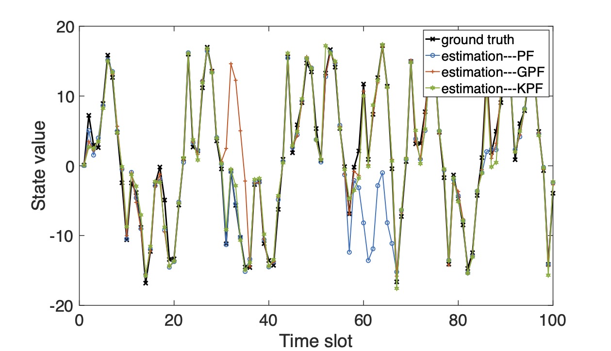
Figure 3: Estimation performance comparison of the PF, GPF, and AKKF filters for the UNGM in 100 time slot, the number of particles is set as $M=20$.

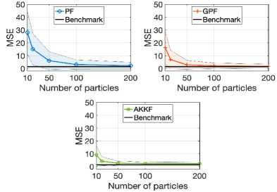
Figure 4: Performance comparison of the PF, GPF, and AKKF filters with an increasing number of particles. Legend: Solid lines are the average MSEover 1000 random MC realizations, i.e., $\mathbb{E}(\mathrm{MSE})$; The colored areas are error bars calculated as $\mathbb{E}(\mathrm{MSE})\pm\mathrm{Std}(\mathrm{MSE})$.

IV-B Bearing-only Tracking (BOT) – Linear Motion Behavior

The BOT problem is of interest for airborne radar and sonar in passive listening mode and electronic warfare systems [14]. This paper considers the BOT problem with one object moving in a 2-D space. The hidden state $\mathbf{x}_{n}=[\xi_{n},\dot{\xi}_{n},\eta_{n},\dot{\eta}_{n}]^{T}$, where $(\xi_{n},\eta_{n})$ and $(\dot{\xi}_{n},\dot{\eta}_{n})$ represent the target position and the corresponding velocity on X-axis and Y-axis, respectively. The moving trajectory is assumed to follow a CV motion model, which is represented as

$$\mathbf{x}_{n}=\mathbf{F}\mathbf{x}_{n-1}+\mathbf{G}\mathbf{u}_{n},\;\;n=1,\dots,N,$$ (54)

where $N=30$, the process noise is a $2\times 1$ vector, i.e., $\mathbf{u}_{n}=\left[u_{x},u_{y}\right]_{n}^{\mathrm{T}}$, which follows a Gaussian distribution $\mathbf{u}_{n}\sim\mathcal{N}(\mathbf{0},\sigma^{2}_{u}\mathbf{I}_{2})$, $\sigma_{u}=1e^{-3}$ and $\mathbf{I}_{2}$ is the $2\times 2$ identity matrix.

$$\mathbf{F}=\begin{bmatrix}1&T_{s}&0&0\\ 0&1&0&0\\ 0&0&1&T_{s}\\ 0&0&0&1\\ \end{bmatrix},\;\;\;\mathbf{G}=\begin{bmatrix}0.5&0\\ 1&0\\ 0&0.5\\ 0&1\\ \end{bmatrix}$$

where $T_{s}$ is the sampling interval and is set as $T_{s}=1$. The prior distribution for the initial state is specified as $\mathbf{x}_{0}\sim\mathcal{N}(\bar{\mathbf{x}}_{0},\mathbf{P}_{0})$. Following [14], we set the parameters of the prior distribution to be $\bar{\mathbf{x}}_{0}=\left[-0.05,0.001,0.7,-0.05\right]^{\mathrm{T}}$ and

$$\mathbf{P}_{0}=\begin{bmatrix}0.1&0&0&0\\ 0&0.005&0&0\\ 0&0&0.1&1\\ 0&0&0&0.01\\ \end{bmatrix}.$$

Although the motion model in this example is linear, the measurement model is non-linear, leading to non-Gaussian state distributions. We model the measurements as the actual bearing with an additional Gaussian error term,

$$y_{n}=\tan^{-1}(\frac{\eta_{n}}{\xi_{n}})+v_{n}.$$ (55)

Here, the inverse tangent is the four-quadrant inverse tangent function, $v_{n}\sim\mathcal{N}(0,\sigma^{2}_{v})$, $\sigma_{v}=5e^{-3}$.

IV-B1 Tracking performance

Fig. 5 displays two representative trajectories and the tracking performance obtained by six filters: UKF, GPF, PF, the proposed AKKF using finite quadratic kernel and quartic kernels, and the proposed AKKF using infinite Gaussian kernel. We locate the observer at $\left[0,0\right]$. The number of particles used for the PF, GPF, and AKKFs is 20. The number of sigma points for the UKF is 19. It can be seen from Fig. 5 that with a small number of particles, divergence may occur for the PF, GPF, and UKF, while divergence is not observed for the proposed AKKFs.

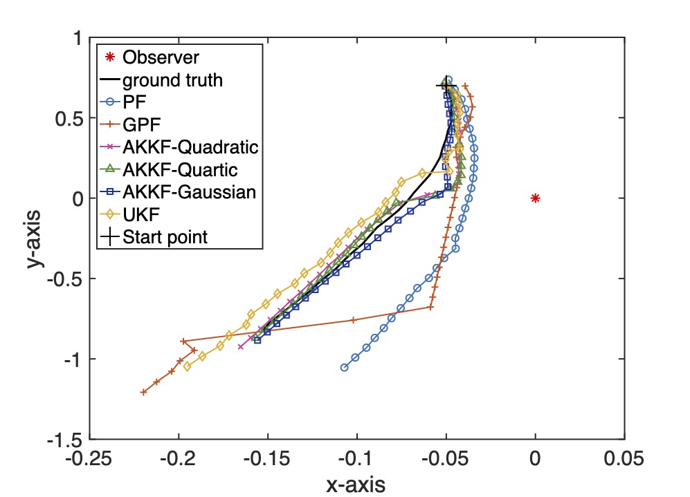
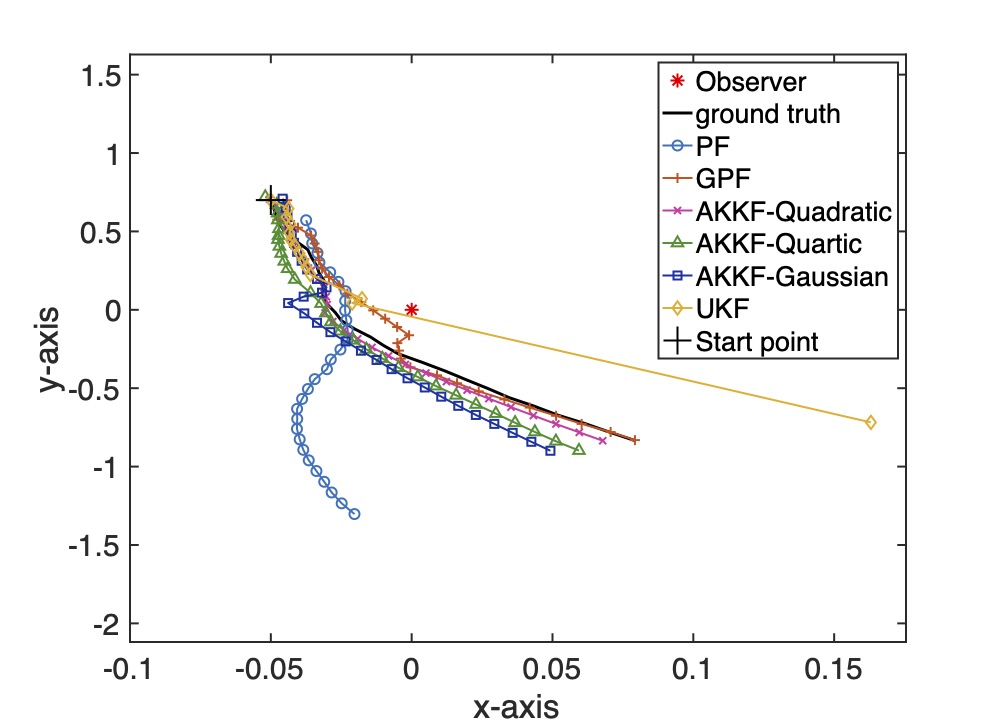
Figure 5: BOT performance of a moving target in two dimensions with UKF, GPF, PF, quadratic kernel-based AKKF, quartic kernel-based AKKF, and Gaussian kernel-based AKKF. The number of particles for GPF, PF, and AKKFs is $M=20$. Legend: $*$: the observer, $+$: the start point of moving trajectory. (a) Trajectory-1, (b) Trajectory-2.

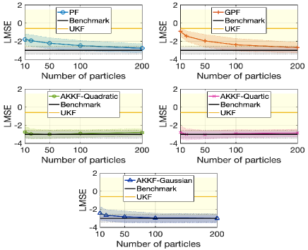
Figure 6: LMSE performance obtained by the UKF, PF, GPF, quadratic kernel-based AKKF, quartic kernel-based AKKF, and Gaussian kernel-based AKKF with an increasing number of particles. Legend: Solid lines are the average value of LMSEs, i.e., $\mathbb{E}(\mathrm{LMSE})$ for 1000 random MC realizations. The colored areas are error bars $\mathbb{E}(\mathrm{LMSE})\pm\mathrm{Std}(\mathrm{LMSE})$.

Fig. 6 shows the average logarithmic mean square error (LMSE) obtained for 1000 random MC realizations for all the position state variables. The LMSE is defined as,

$$\mathrm{LMSE}=\log\left[\frac{1}{N}\sum_{n=1}^{N}\sqrt{(\xi_{n}-\hat{\xi}_{n})^{2}+(\eta_{n}-\hat{\eta}_{n})^{2}}\right].$$ (56)

The numbers of particles are set to be $M=\left[10,20,50,100,200\right]$. The compared filters are the PF, the GPF, and the AKKFs using quadratic kernel, quartic kernel, and Gaussian kernel, respectively. The benchmark performance is achieved by the bootstrap PF with $10^{4}$ particles. From Fig. 6, we arrive at the following conclusions. First, the proposed AKKFs show significant improvement compared to the PF and GPF with the same number of particles, especially with small numbers of particles, i.e., $M=\left[10,20,50\right]$. Second, on average, the AKKF using the quartic kernel performs better than the AKKF using the quadratic kernel. The improved performance is likely due to the quartic feature mappings incorporating more statistical information about the hidden state. The AKKFs using quadratic and quartic kernels can approach the benchmark performance with 20 particles. It is interesting that the LMSE performance slightly deteriorates here as the number of particles increases. This appears to be caused by the overuse of particles, which is likely to lead to singular or badly scaled Gram matrices, increasing the inaccuracy of matrix inversion. Hence, estimation biases propagate to reduce the tracking performance.

Next, we investigate the effects of varying regularization parameters $\lambda$ and $\kappa$ on the tracking performance. The former is used in the calculation of the transition matrix $\Gamma_{n}$ in (31). The latter is used for the calculation of kernel Kalman gain $Q_{n}$ in (47). The regularization parameter choice must be derived from the real data. Hence, we investigate the good empirical value of regularization parameters using an MC method. In this simulation, $\kappa$ is set to be equal to $\lambda$, and the number of particles for AKKF is set to be 50. From Fig. 7, we can see that the LMSE performance is relatively insensitive to the values of $\lambda$ and $\kappa$ when they are in the range $\left[10^{-4},10^{-2}\right]$.

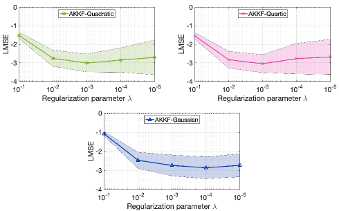
Figure 7: LMSE performance comparison of the PF, GPF, and AKKF filters with the varying regularization parameter $\lambda$. The number of MC random realizations is set to 1000. Legend: Solid lines are the average over 1000 random MC realizations, i.e., $\mathbb{E}(\mathrm{MSE})$. The colored areas are error bars calculated as $\mathbb{E}(\mathrm{MSE})\pm\mathrm{Std}(\mathrm{MSE})$.

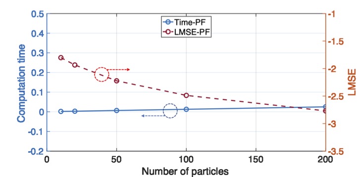
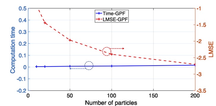
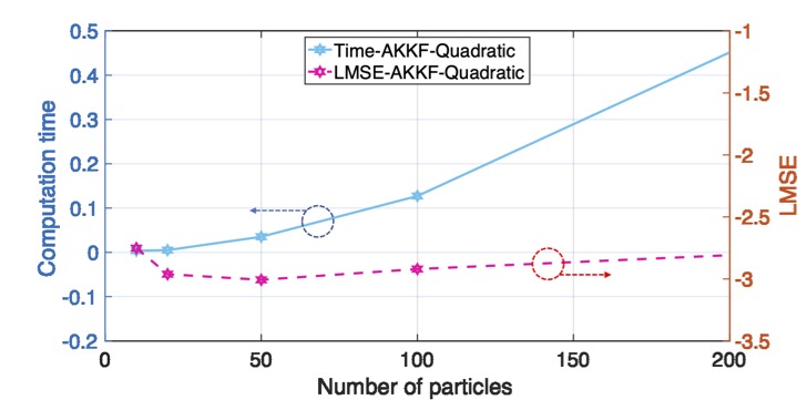
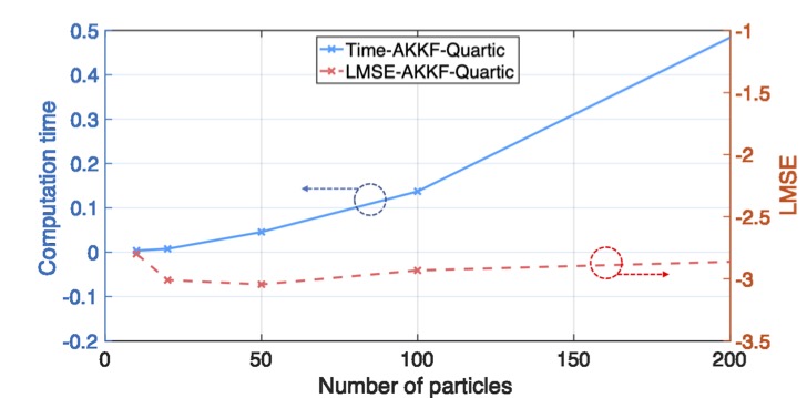
Figure 8: Showing the trend of the computation time and LMSE of the PF, GPF, and different AKKFs; Average computation time (s) and LMSE over 1000 MC random realizations with increasing number of particles. Legend: Blue circles with arrows mean that the curves are the performance of computation time; Red circles with arrows mean that the curves show the LMSE performance.

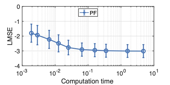
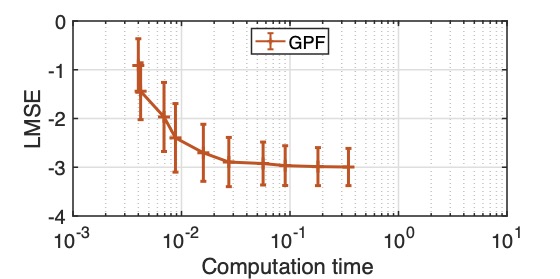
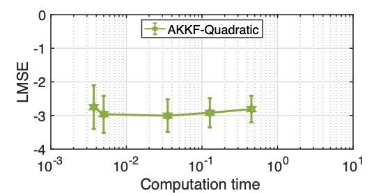
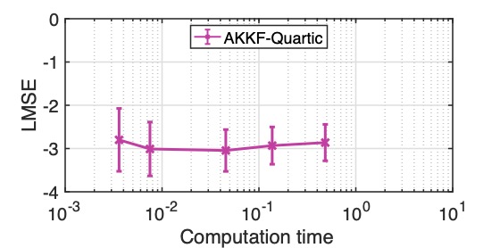
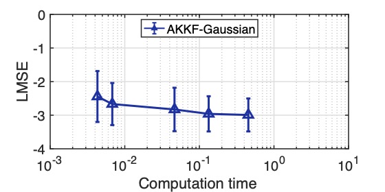
Figure 9: Computation time and LMSE; Average computation time (s) and LMSE over 1000 MC random realizations.

IV-B2 Computational complexity

In the next experiment, we compare the computation time of filters and show the results in Fig. 8. The simulations are implemented in Matlab and run using MacBook Pro, Chip Apple M1. Fig. 8 shows the average computation time obtained for 1000 MC realizations, from which we can see that the computation time of the bootstrap PF increases linearly with the increase of particle numbers, while the computation time of the proposed AKKF increases quadratically with the increase of particle numbers $M$ when $10\leq M\leq 200$, since the computational complexity of matrices inversion increases quadratically. Even though the increasing trend of computational complexity for the AKKF is more significant, the LMSE tracking performance of the AKKF can approach the benchmark, e.g., $-3.0$, with very small number of particles requirement. For a further confirmation of this conclusion, Fig. 9 shows the LMSE performance with the correspond running time. From this figure, we can conclude that with the LMSE performance benchmark is $-3.0$, the computation time for the PF, GPF, quadratic kernel-based AKKF, quartic kernel-based AKKF and Gaussian kernel-based AKKF are 0.35s, 0.35s, 0.035s, 0.0075s and 0.45s, respectively.

IV-C Bearing-only Tracking (BOT) – Highly Maneuvering Behaviors

In our final experiment, we consider the same BOT observation model with a nonlinear motion model. The motion behavior of hidden states $\mathbf{x}_{n}=\left[\xi_{n},\dot{\xi}_{n},\eta_{n},\dot{\eta}_{n},\omega_{n}\right]^{\mathrm{T}},n=1,\dots,N$ is set to follow CT model with unknown and dynamic turn rate as [31]

$$\begin{split}\begin{bmatrix}\xi_{n}\\ \dot{\xi}_{n}\\ \eta_{n}\\ \dot{\eta}_{n}\end{bmatrix}=\begin{bmatrix}&1&\frac{\sin\omega_{n-1}T_{s}}{\omega_{n-1}}&0&-\frac{1-\cos\omega_{n-1}T_{s}}{\omega_{n-1}}\\ &0&\cos\omega_{n-1}T_{s}&0&-\sin\omega_{n-1}T_{s}\\ &0&\frac{1-\cos\omega_{n-1}T_{s}}{\omega_{n-1}}&1&\frac{\sin\omega_{n-1}T_{s}}{\omega_{n-1}}\\ &0&\sin\omega_{n-1}T_{s}&0&\cos\omega_{n-1}T_{s}\\ \end{bmatrix}\mathbf{x}_{n-1}+\mathbf{v}_{n},\end{split}$$ (57)

$$\omega_{n}=\begin{cases}\omega_{n-1}+v_{n,\omega},&\text{if }n\neq N/2\\ \omega_{n-1}/3+v_{n,\omega},&\text{otherwise}\end{cases}$$ (58)

where $\omega_{n}$ is the random walk turn rate and changes at $n=N/2$. The sampling interval is set as $T_{s}=1$, $\mathbf{v}_{n}\sim\mathcal{N}(\mathbf{0},\sigma^{2}_{v}R)$, $v_{n,\omega}\sim\mathcal{N}({0},\sigma^{2}_{w})$, $\sigma_{v}=1e^{-3}$, and $\sigma_{\omega}=1e^{-2}$,

$$\begin{split}&R=\\ &\begin{bmatrix}&\frac{2(\omega_{n}T_{s}-\sin\omega_{n}T_{s})}{\omega_{n}^{3}}&\frac{1-\cos\omega_{n}T_{s}}{\omega_{n}^{2}}&0&\frac{\omega_{n}T_{s}-\sin\omega_{n}T_{s}}{\omega_{n}^{2}}\\ &\frac{1-\cos\omega_{n}T_{s}}{\omega_{n}^{2}}&T_{s}&-\frac{\omega_{n}T_{s}-\sin\omega_{n}T_{s}}{\omega_{n}^{3}}&0\\ &0&-\frac{\omega_{n}T_{s}-\sin\omega_{n}T_{s}}{\omega_{n}^{3}}&\frac{2(\omega_{n}T_{s}-\sin\omega_{n}T_{s})}{\omega_{n}^{3}}&\frac{1-\cos\omega_{n}T_{s}}{\omega_{n}^{2}}\\ &\frac{\omega_{n}T_{s}-\sin\omega_{n}T_{s}}{\omega_{n}^{2}}&0&\frac{1-\cos\omega_{n}T_{s}}{\omega_{n}^{2}}&T_{s}\end{bmatrix}.\end{split}$$

The initial position and velocity states’ prior distribution follows the settings in Section IV-B. The prior distribution for the unknown turn rate is $\omega_{0}\sim\mathcal{U}\left[0,\pi/6\right]$. The measurement model and corresponding settings follow (55).

Figure 10: Tracking performance of a moving target following CT model with random walk turn rate. The number of particles for GPF, PF, and AKKFs is $M=100$. Legend: $*$: the observer, $+$: the start point of moving trajectory. (a) Trajectory-1, (b) Trajectory-2.

Fig. 10 displays two representative trajectories and the tracking performance obtained by six filters: UKF, GPF, PF, the AKKF with quadratic, quartic and Gaussian kernels. The PF with $10^{4}$ particles is used as a benchmark. The number of particles used for the compared PF, GPF, and AKKFs is 100. The number of sigma points for the UKF is 23. Fig. 11 shows the average LMSE obtained for 1000 random MC realizations for all the position state variables. We set the numbers of particles as $M=\left[20,50,100,200\right]$. From Fig. 10 and Fig. 11, we conclude that divergence is more severe for the PF, GPF, and UKF than the proposed AKKFs, and the proposed AKKFs still significantly improve performance with small numbers of particles when the target is undergoing non-linear motion behavior. However, the performance of the AKKFs with quadratic and quartic kernels can’t be enhanced with the increased number of particles when $M>50$. This appears to be caused by the fact that quadratic and quartic kernels only allow modeling features of data up to the order of the polynomial, but for the BOT systems in which the target behaves following highly maneuvering, quadratic and quartic kernels are not effective enough to capture the diversity of the non-linearities.

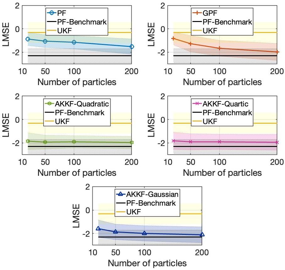
Figure 11: LMSE performance for the BOT tracking under the CT model with unknown and random walk turn rate. Legend: Solid lines are the average value of LMSEs, i.e., $\mathbb{E}(\mathrm{LMSE})$ for 1000 random MC realizations. The colored areas are error bars $\mathbb{E}(\mathrm{LMSE})\pm\mathrm{Std}(\mathrm{LMSE})$.

V Conclusions

In this paper, we provided a new approach to model-driven Bayesian filters. By embedding the predictive and posterior pdfs into RKHSs, classical KF calculation can be employed along with an adaptive sampling of the DSSM to predict the new data space information. We have observed that more feature information of the hidden states and the observations can be captured and recorded with a significantly smaller number of particles than are needed in PF-based methods while retaining equivalent estimation accuracy. Furthermore, as the new filters are comprised of standard matrix-vector multiplication operations, the overall computational complexity is also very favorable and offers an excellent opportunity for parallelization.

This Appendix gives the derivations of kernel Kalman gain $\mathcal{Q}_{n}$ and updated kernel covariance operator $\hat{\mathcal{C}}_{x_{n}x_{n}}^{+}$ that follow [23] but are included here for completeness.

The trace of the posteriori covariance operator $\hat{\mathcal{C}}_{\mathbf{x}_{n}\mathbf{x}_{n}}^{+}$ is defined as $\hat{\mathcal{C}}_{\mathbf{x}_{n}\mathbf{x}_{n}}^{+}=\mathbb{E}\left[\epsilon_{n}\epsilon_{n}^{\rm{T}}\right]$, where $\epsilon_{n}$ is the error of the posteriori KME and calculated as

$$\epsilon_{n} =\phi_{\mathbf{x}}(\mathbf{x}_{n})-\hat{\mu}_{\mathbf{x}_{n}}^{+}$$ (59)

$$=\phi_{\mathbf{x}}(\mathbf{x}_{n})-\left[\hat{\mu}_{\mathbf{x}_{n}}^{-}+\mathcal{Q}_{n}\left(\phi_{\mathbf{y}}(\mathbf{y}_{n})-\hat{\mathcal{C}}_{\mathbf{y}_{n}|\mathbf{x}_{n}}\hat{\mu}_{\mathbf{x}_{n}}^{-}-\mathcal{R}\right)\right]$$

$$=\left(I-\mathcal{Q}_{n}\hat{\mathcal{C}}_{\mathbf{y}_{n}|\mathbf{x}_{n}}\right)\left(\phi_{\mathbf{x}}(\mathbf{x}_{n})-\hat{\mu}_{\mathbf{x}_{n}}^{-}\right)-\mathcal{Q}_{n}\mathcal{R},$$

where we have used the fact that $\phi_{\mathbf{y}}(\mathbf{y}_{n})=\mathcal{C}_{\mathbf{y}_{n}|\mathbf{x}_{n}}\phi_{\mathbf{x}}(\mathbf{x}_{n})$. Then, noting that $\phi_{\mathbf{x}}(\mathbf{x}_{n-1})-\hat{\mu}_{\mathbf{x}_{n-1}}^{+}=\epsilon_{n-1}$, $\hat{\mathcal{C}}_{\mathbf{x}_{n}\mathbf{x}_{n}}^{+}$ is calculated as

$$\hat{\mathcal{C}}_{\mathbf{x}_{n}\mathbf{x}_{n}}^{+}=\left(I-\mathcal{Q}_{n}\hat{\mathcal{C}}_{\mathbf{y}_{n}|\mathbf{x}_{n}}\right)\hat{\mathcal{C}}_{\mathbf{x}_{n}\mathbf{x}_{n}}^{-}\left(I-\mathcal{Q}_{n}\hat{\mathcal{C}}_{\mathbf{y}_{n}|\mathbf{x}_{n}}\right)^{\mathrm{T}}+\mathcal{Q}_{n}\mathcal{R}\mathcal{Q}_{n}^{\mathrm{T}},$$ (60)

where $\mathcal{R}$ is the covariance matrix of the residual of the observation operator. The trace of $\hat{\mathcal{C}}_{\mathbf{x}_{n}\mathbf{x}_{n}}^{+}$ is minimized when its matrix derivative with respect to the gain matrix is zero.

$$\frac{\partial\hat{\mathcal{C}}_{\mathbf{x}_{n}\mathbf{x}_{n}}^{+}}{\partial\mathcal{Q}_{n}}=-2(I-\mathcal{Q}_{n}\hat{\mathcal{C}}_{\mathbf{y}_{n}|\mathbf{x}_{n}})\hat{\mathcal{C}}_{\mathbf{x}_{n}\mathbf{x}_{n}}^{-}\hat{\mathcal{C}}_{\mathbf{y}_{n}|\mathbf{x}_{n}}^{\mathrm{T}}+2\mathcal{Q}_{n}\mathcal{R}=0$$ (61)

$$\Rightarrow \mathcal{Q}_{n}=\hat{\mathcal{C}}_{\mathbf{x}_{n}\mathbf{x}_{n}}^{-}\mathcal{C}_{\mathbf{y}_{n}|\mathbf{x}_{n}}^{\mathrm{T}}\left(\hat{\mathcal{C}}_{\mathbf{y}_{n}|\mathbf{x}_{n}}\hat{\mathcal{C}}_{\mathbf{x}_{n}\mathbf{x}_{n}}^{-}\hat{\mathcal{C}}_{\mathbf{y}_{n}|\mathbf{x}_{n}}^{\mathrm{T}}+\mathcal{R}\right)^{-1},$$

where $\hat{\mathcal{C}}_{\mathbf{x}_{n}\mathbf{x}_{n}}^{-}$ is the predictive kernel covariance operator and is calculated by (33), $\hat{\mathcal{C}}_{\mathbf{y}_{n}|\mathbf{x}_{n}}$ is the empirical likelihood operator and is calculated as

$$\hat{\mathcal{C}}_{\mathbf{y}_{n}|\mathbf{x}_{n}} =\Upsilon_{n}\left(\Phi_{n}^{\mathrm{T}}\Phi_{n}+\lambda_{K}I\right)^{-1}\Phi_{n}^{\mathrm{T}}$$ (62)

$$=\Upsilon_{n}\left(K_{\mathbf{x}\mathbf{x}}+\lambda_{K}I\right)^{-1}\Phi_{n}^{\mathrm{T}}.$$

Here, the Gram matrix $K_{\mathbf{x}\mathbf{x}}=\Phi_{n}^{\mathrm{T}}\Phi_{n}$, and $\lambda_{{K}}$ is the regularization parameter to modify $K_{\mathbf{x}\mathbf{x}}$. In this paper, $\lambda_{{K}}$ is set to be 0. $\mathcal{R}$ is set as $\mathcal{R}=\kappa I$, $\kappa$ is used to approximate the covariance of the residual of the observation operator.

Combine (39) and (62), we can have the following reductions,

$$\hat{\mathcal{C}}_{\mathbf{x}_{n}\mathbf{x}_{n}}^{-}\hat{\mathcal{C}}_{\mathbf{y}_{n}|\mathbf{x}_{n}}^{\mathrm{T}}$$ (63)

$$=\left[\Phi_{n}(\tilde{S}_{n-1}^{+}+V_{n})\Phi_{n}^{\mathrm{T}}\right]\left[\Upsilon_{n}\left(K_{\mathbf{x}\mathbf{x}}+\lambda_{K}I\right)^{-1}\Phi_{n}^{\mathrm{T}}\right]^{\mathrm{T}}$$

$$=\Phi_{n}S_{n}^{-}\left[\left(K_{\mathbf{x}\mathbf{x}}+\lambda_{K}I\right)^{-1}\Phi_{n}^{\mathrm{T}}\Phi_{n}\right]^{\mathrm{T}}\Upsilon_{n}^{\mathrm{T}}$$

$$=\Phi_{n}S_{n}^{-}\left[\left(K_{\mathbf{x}\mathbf{x}}+\lambda_{K}I\right)^{-1}K_{\mathbf{x}\mathbf{x}}\right]^{\mathrm{T}}\Upsilon_{n}^{\mathrm{T}}$$

$$\overset{\lambda_{K}=0}{=\joinrel=}\Phi_{n}S_{n}^{-}\Upsilon_{n}^{\mathrm{T}},$$

$$\mathcal{C}_{\mathbf{y}_{n}|\mathbf{x}_{n}}\mathcal{C}_{\mathbf{x}_{n}\mathbf{x}_{n}}^{-}\mathcal{C}_{\mathbf{y}_{n}|\mathbf{x}_{n}}^{\mathrm{T}}$$ (64)

$$=\left[\Upsilon_{n}\left(K_{\mathbf{x}\mathbf{x}}+\lambda_{K}I\right)^{-1}\Phi_{n}^{\mathrm{T}}\right]\left(\Phi_{n}S_{n}^{-}\Phi_{n}^{\mathrm{T}}\right)\left[\Upsilon_{n}\left(K_{\mathbf{x}\mathbf{x}}+\lambda_{K}I\right)^{-1}\Phi_{n}^{\mathrm{T}}\right]^{\mathrm{T}}$$

$$=\Upsilon_{n}\left[\left(K_{\mathbf{x}\mathbf{x}}+\lambda_{K}I\right)^{-1}K_{\mathbf{x}\mathbf{x}}\right]S_{n}^{-}\left[\left(K_{\mathbf{x}\mathbf{x}}+\lambda_{K}I\right)^{-1}K_{\mathbf{x}\mathbf{x}}\right]^{\mathrm{T}}\Upsilon_{n}^{\mathrm{T}}$$

$$\overset{\lambda_{K}=0}{=\joinrel=}\Upsilon_{n}S_{n}^{-}\Upsilon_{n}^{\mathrm{T}}.$$

Substitute (63) and (64) into (61), the AKKF gain $\mathcal{Q}_{n}$ can be calculated as,

$$\mathcal{Q}_{n} =\hat{\mathcal{C}}_{\mathbf{x}_{n}\mathbf{x}_{n}}^{-}\mathcal{C}_{\mathbf{y}_{n}|\mathbf{x}_{n}}^{\mathrm{T}}\left(\hat{\mathcal{C}}_{\mathbf{y}_{n}|\mathbf{x}_{n}}\hat{\mathcal{C}}_{\mathbf{x}_{n}\mathbf{x}_{n}}^{-}\hat{\mathcal{C}}_{\mathbf{y}_{n}|\mathbf{x}_{n}}^{\mathrm{T}}+\mathcal{R}\right)^{-1}$$ (65)

$$=\Phi_{n}S_{n}^{-}\Upsilon_{n}^{\mathrm{T}}\left(\Upsilon_{n}S_{n}^{-}\Upsilon_{n}^{\mathrm{T}}+\kappa I\right)^{-1}$$

$$=\Phi_{n}S_{n}^{-}\Upsilon_{n}^{\mathrm{T}}\left(\Upsilon_{n}^{\mathrm{T}}\right)^{-1}\left[\Upsilon_{n}^{\mathrm{T}}\Upsilon_{n}S_{n}^{-}\Upsilon_{n}^{\mathrm{T}}\left(\Upsilon_{n}^{\mathrm{T}}\right)^{-1}+\Upsilon_{n}^{\mathrm{T}}\kappa I\left(\Upsilon_{n}^{\mathrm{T}}\right)^{-1}\right]^{-1}\Upsilon_{n}^{\mathrm{T}}$$

$$=\Phi_{n}S_{n}^{-}\left(G_{\mathbf{y}\mathbf{y}}S_{n}^{-}+\kappa I\right)^{-1}\Upsilon_{n}^{\mathrm{T}}.$$

The covariance operator $\hat{\mathcal{C}}_{\mathbf{x}_{n}\mathbf{x}_{n}}^{+}$ in (60) is further derived as

$$\hat{\mathcal{C}}_{\mathbf{x}_{n}\mathbf{x}_{n}}^{+}= \left(I-\mathcal{Q}_{n}\hat{\mathcal{C}}_{\mathbf{y}_{n}|\mathbf{x}_{n}}\right)\hat{\mathcal{C}}_{\mathbf{x}_{n}\mathbf{x}_{n}}^{-}\left(I-\mathcal{Q}_{n}\hat{\mathcal{C}}_{\mathbf{y}_{n}|\mathbf{x}_{n}}\right)^{\mathrm{T}}+\mathcal{Q}_{n}\mathcal{R}\mathcal{Q}_{n}^{\mathrm{T}}$$ (66)

$$= \hat{\mathcal{C}}_{\mathbf{x}_{n}\mathbf{x}_{n}}^{-}-\hat{\mathcal{C}}_{\mathbf{x}_{n}\mathbf{x}_{n}}^{-}\hat{\mathcal{C}}_{\mathbf{y}_{n}|\mathbf{x}_{n}}^{\rm{T}}\mathcal{Q}_{n}^{\mathrm{T}}-\mathcal{Q}_{n}\hat{\mathcal{C}}_{\mathbf{y}_{n}|\mathbf{x}_{n}}\hat{\mathcal{C}}_{\mathbf{x}_{n}\mathbf{x}_{n}}^{-}$$

$$+\mathcal{Q}_{n}\hat{\mathcal{C}}_{\mathbf{y}_{n}|\mathbf{x}_{n}}\hat{\mathcal{C}}_{\mathbf{x}_{n}\mathbf{x}_{n}}^{-}\hat{\mathcal{C}}_{\mathbf{y}_{n}|\mathbf{x}_{n}}^{\rm{T}}\mathcal{Q}_{n}^{\mathrm{T}}+\mathcal{Q}_{n}\mathcal{R}\mathcal{Q}_{n}^{\mathrm{T}}$$

$$= \hat{\mathcal{C}}_{\mathbf{x}_{n}\mathbf{x}_{n}}^{-}-\Phi_{n}S_{n}^{-}\Upsilon_{n}^{\mathrm{T}}\mathcal{Q}_{n}^{\mathrm{T}}-\mathcal{Q}_{n}\Upsilon_{n}S_{n}^{-}\Phi_{n}^{\mathrm{T}}+\mathcal{Q}_{n}\left(\Upsilon_{n}S_{n}^{-}\Upsilon_{n}^{\mathrm{T}}+\mathcal{R}\right)\mathcal{Q}_{n}^{\mathrm{T}}$$

$$= \hat{\mathcal{C}}_{\mathbf{x}_{n}\mathbf{x}_{n}}^{-}-\Phi_{n}S_{n}^{-}\Upsilon_{n}^{\mathrm{T}}\mathcal{Q}_{n}^{\mathrm{T}}-\mathcal{Q}_{n}\Upsilon_{n}S_{n}^{-}\Phi_{n}^{\mathrm{T}}$$

$$+\Phi_{n}S_{n}^{-}\Upsilon_{n}^{\mathrm{T}}\left(\Upsilon_{n}S_{n}^{-}\Upsilon_{n}^{\mathrm{T}}+\kappa I\right)^{-1}\left(\Upsilon_{n}S_{n}^{-}\Upsilon_{n}^{\mathrm{T}}+\kappa I\right)\mathcal{Q}_{n}$$

$$= \hat{\mathcal{C}}_{\mathbf{x}_{n}\mathbf{x}_{n}}^{-}-\mathcal{Q}_{n}\Upsilon_{n}S_{n}^{-}\Phi_{n}^{\mathrm{T}}.$$

References

- [1] M. S. Grewal and A. P. Andrews, Kalman Filtering: Theory and Practice With MATLAB, 3rd ed. Hoboken, NJ, USA: Wiley, 2008.
- [2] S. J. Julier, J. K. Uhlmann, and H. F. Durrant-Whyte, “A new approach for filtering nonlinear systems,” in Proceedings of 1995 American Control Conference - ACC’95, vol. 3, 1995, pp. 1628–1632.
- [3] E. A. Wan and R. Van Der Merwe, “The unscented Kalman filter for nonlinear estimation,” in Proceedings of the IEEE 2000 Adaptive Systems for Signal Processing, Communications, and Control Symposium (Cat. No.00EX373), 2000, pp. 153–158.
- [4] N. Gordon, D. Salmond, and C. Ewing, “Bayesian state estimation for tracking and guidance using the bootstrap filter,” J. Guid. Control. Dyn., vol. 18, pp. 1434–1443, 1995.
- [5] M. Kanagawa, Y. Nishiyama, A. Gretton, and K. Fukumizu, “Filtering with state-observation examples via kernel Monte Carlo filter,” Neural Comput., vol. 28, no. 2, pp. 382–444, 2016.
- [6] M. Kanagawa, Y. Nishiyama, A. Gretton, and K. Fukumizu, “Monte Carlo filtering using kernel embedding of distributions,” in AAAI, 2014.
- [7] M. Sun, M. E. Davies, I. Proudler, and J. R. Hopgood, “A Gaussian process based method for multiple model tracking,” in 2020 Sensor Signal Processing for Defence Conference (SSPD), 2020, pp. 1–5.
- [8] M. S. Arulampalam, S. Maskell, N. Gordon, and T. Clapp, “A tutorial on particle filters for online nonlinear/non-gaussian Bayesian tracking,” IEEE Trans. Signal Process, vol. 50, no. 2, pp. 174–188, 2002.
- [9] B.-T. Vo and B.-N. Vo, “Labeled random finite sets and multi-object conjugate priors,” IEEE Trans. Signal Process, vol. 61, no. 13, pp. 3460–3475, 2013.
- [10] H. W. Sorenson, Kalman Filtering: Theory and Application. NJ: IEEE: Piscataway, 1985.
- [11] S. J. Julier and J. K. Uhlmann, “New extension of the Kalman filter to nonlinear systems,” in Signal Processing, Sensor Fusion, and Target Recognition VI, I. Kadar, Ed., vol. 3068, International Society for Optics and Photonics. SPIE, 1997, pp. 182 – 193. [Online]. Available: https://doi.org/10.1117/12.280797
- [12] S. Julier and J. K. Uhlmann, “A general method for approximating nonlinear transformations of probability distributions,” Eng. Dept.,Univ. Oxford, Oxford, U.K., Tech. Rep., 1996.
- [13] K. Ito and K. Xiong, “Gaussian filters for nonlinear filtering problems,” IEEE Trans. Autom. Control., vol. 45, pp. 910–927, 2000.
- [14] J. H. Kotecha and P. M. Djuric, “Gaussian particle filtering,” IEEE Trans. Signal Process, vol. 51, no. 10, pp. 2592–2601, 2003.
- [15] A. Doucet, S. Godsill, and C. Andrieu, “On sequential Monte Carlo sampling methods for Bayesian filtering,” Stat. Comput., vol. 10, 04 2003.
- [16] J. H. Kotecha and P. M. Djuric, “Sequential Monte Carlo sampling detector for Rayleigh fast-fading channels,” in 2000 IEEE International Conference on Acoustics, Speech, and Signal Processing. Proceedings (Cat. No.00CH37100), vol. 1, 2000, pp. 61–64 vol.1.
- [17] T. Li, M. Bolic, and P. M. Djuric, “Resampling methods for particle filtering: Classification, implementation, and strategies,” IEEE Signal Process. Mag., vol. 32, no. 3, pp. 70–86, 2015.
- [18] Dong Guo and Xiaodong Wang, “Quasi-monte carlo filtering in nonlinear dynamic systems,” IEEE Trans. Signal Process, vol. 54, no. 6, pp. 2087–2098, 2006.
- [19] P. Closas, C. Fernandez-Prades, and J. Vila-Valls, “Multiple quadrature Kalman filtering,” IEEE Trans. Signal Process, vol. 60, no. 12, pp. 6125–6137, 2012.
- [20] P. Stano, Z. Lendek, J. Braaksma, R. Babuška, C. de Keizer, and A. J. den Dekker, “Parametric Bayesian filters for nonlinear stochastic dynamical systems: A survey,” IEEE Trans. Cybern., vol. 43, no. 6, pp. 1607–1624, 2013.
- [21] L. Song, K. Fukumizu, and A. Gretton, “Kernel embeddings of conditional distributions: A unified kernel framework for nonparametric inference in graphical models,” IEEE Signal Process. Mag., vol. 30, no. 4, pp. 98–111, 2013.
- [22] K. Fukumizu, L. Song, and A. Gretton, “Kernel Bayes’ rule: Bayesian inference with positive definite kernels,” J. Mach. Learn. Res., vol. 14, no. 1, p. 3753–3783, Dec. 2013.
- [23] G. Gebhardt, A. Kupcsik, and G. Neumann , “The kernel Kalman rule,” Mach. Learn., pp. 2113–2157, 2019.
- [24] M. Sun, M. E. Davies, I. Proudler, and J. R. Hopgood, “Adaptive kernel Kalman filter,” in 2021 Sensor Signal Processing for Defence Conference (SSPD), 2021, pp. 1–5.
- [25] M. Sun, M. E. Davies, I. K. Proudler, and J. R. Hopgood, “Adaptive kernel Kalman filter multi-sensor fusion,” in 24th International Conference on Information Fusion, 2021, pp. 1–8.
- [26] K. Fukumizu, F. R. Bach, and M. I. Jordan, “Kernel dimension reduction in regression,” The Annals of Statistics, vol. 37, no. 4, pp. 1871 – 1905, 2009. [Online]. Available: https://doi.org/10.1214/08-AOS637
- [27] G. Gebhardt, A. Kupcsik, and G. Neumann, “The kernel Kalman rule: efficient nonparametric inference with recursive least squares,” in Thirty-First AAAI Conference on Artificial Intelligence, vol. 1, Feb. 2017, pp. 4–9.
- [28] Y. Chen, M. Welling, and A. Smola, “Super-samples from kernel herding,” in UAI, 2010.
- [29] M. Alama, H. Lin, H. Deng, V. D. Calhound, and W. Yuping, “A kernel machine method for detecting higher order interactions in multimodal datasets: Application to schizophrenia,” J. Neurosci. Methods, vol. 1, no. 309, pp. 161–174, 2018.
- [30] S. Grünewälder, G. Lever, A. Gretton, L. Baldassarre, S. Patterson, and M. Pontil, “Conditional mean embeddings as regressors,” in ICML, 2012.
- [31] X. Rong Li and V. Jilkov, “Survey of maneuvering target tracking. part i. dynamic models,” IEEE Trans. Aerosp. Electron. Syst., vol. 39, no. 4, pp. 1333–1364, 2003.
- [32] O. Cappe, S. J. Godsill, and E. Moulines, “An overview of existing methods and recent advances in sequential Monte Carlo,” Proc. IEEE, vol. 95, no. 5, pp. 899–924, 2007.
- [33] A. Farina, “Target tracking with bearings – only measurements,” Signal Processing, vol. 78, no. 1, pp. 61 – 78, 1999. [Online]. Available: http://www.sciencedirect.com/science/article/pii/S016516849900047X
- [34] S. Julier and J. Uhlmann, “A non-divergent estimation algorithm in the presence of unknown correlations,” in Proceedings of the 1997 American Control Conference (Cat. No.97CH36041), vol. 4, 1997, pp. 2369–2373 vol.4.