Modeling of Asymptotically Periodic Outbreaks:
a long-term SIRW2 description of Covid-19?

Abstract

As the outbreak of COVID-19 enters its third year, we have now enough data to analyse the behavior of the pandemic with mathematical models over a long period of time. The pandemic alternates periods of high and low infections, in a way that sheds a light on the nature of mathematical model that can be used for reliable predictions. The main hypothesis of the model presented here is that the oscillatory behavior is a structural feature of the outbreak, even without postulating a time-dependence of the coefficients. As such, it should be reflected by the presence of limit cycles as asymptotic solutions. This stems from the introduction of (i) a non-linear waning immunity based on the concept of immunity booster (already used for other pathologies); (ii) a fine description of the compartments with a discrimination between individuals infected/vaccinated for the first time, and individuals already infected/vaccinated, undergoing to new infections/doses. We provide a proof-of-concept that our novel model is capable of reproducing long-term oscillatory behavior of many infectious diseases, and, in particular, the periodic nature of the waves of infection. Periodic solutions are inherent to the model, and achieved without changing parameter values in time. This may represent an important step in the long-term modeling of COVID-19 and similar diseases, as the natural, unforced behavior of the solution shows the qualitative characteristics observed during the COVID-19 pandemic.

1 Introduction

It has been two years now that the world experienced the COVID-19 pandemic. We have enough data to identify some patterns in the evolution of the outbreak over time. In particular, in many situations it is evident that the outbreak features an oscillatory behavior, showing an alternating behavior of high and low infected populations. For example, in Fig. 1, we plot the infected curve in Italy (source: [1]). We also plot a Fourier spectral analysis of the data, showing that the dominant frequencies are around 1 year^-1 and three months^-1. Whether this is the effect of a seasonal infection-rate, government measures, or a structural nature of the pandemic is currently an open question.

The calibration of mathematical models with a predictive purpose can be widely educated by the answer to this question. If we assume that the periodicity is a structural feature of the pandemic, a mathematical model should reflect this in the nature of its asymptotic solutions. On the contrary, if the periodicity is the result of seasonality, or government responses to the pandemic (such as lockdowns and masking mandates), the model should incorporate this effect in its parameter calibration.

In the majority of work modeling COVID-19, this latter assumption is employed. Such works typically adopt classical compartmental models like SIR (Susceptible-Infected-Recovered, see [2, 3] for detailed discussion), and its derivations. These models may lead to excellent short-term predictions; however, as they do not have periodic solutions as asymptotic time limit, they will ultimately fail to yield a periodic solution when using time-independent parameters - they do not have periodic asymptotic solutions [4]. In order to recover the observed periodic behavior, then, such models must employ time-dependent parameter fitting, generally attributing the periodicity to underlying changes in population behavior, seasonality, government measures, and other factors [5, 6, 7, 8, 9]. In contrast, in order to recover a truly periodic solution without regular re-parameterization, the presence of limit-cycles becomes a mandatory aspect of long-term modeling.

It is worth noting that the two different possible answers (nature of the problem vs. time-dependence of the parameters) are not mutually exclusive. Looking at the spectral analysis of the Italian data, we argue that it may be a combination of different effects on long and short time scales.

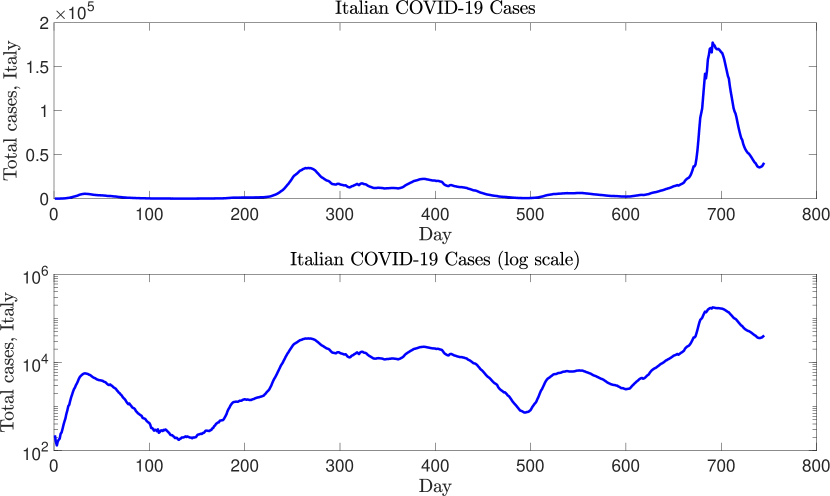
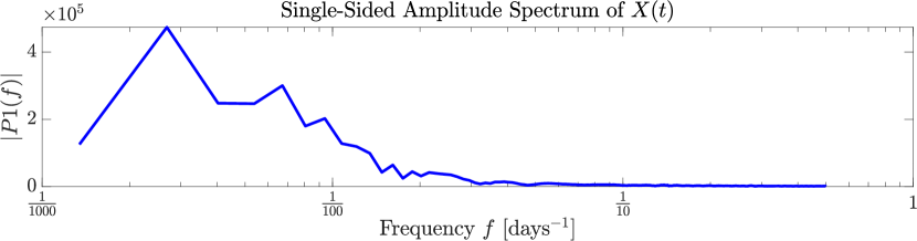
Figure 1: Infected population in Italy over the time range Feb 24 2020- Mar 9 2022. Top: linear scale, center: log-scale. We observe a clear oscillatory, periodic dynamics. Bottom: Fourer spectral analysis showing the dominant frequencies (1/370 days and 1/148 days).

In this paper, we focus on a model where the wavy pattern is primarily intrinsic to the infection qualitatively, acknowledging that behavioral, seasonal, and other external aspects (e.g., higher infectivity in Winter, lower in Summer, different infectivity of different variants, lockdowns) impact the pattern quantitatively.

Our starting point is the concept of waning immunity advocated for other pathologies [10]. Waning Immunity has been already considered for COVID-19, see, e.g., [11, 12, 13, 14] with different mathematical descriptions. The basic idea is that the immunity induced by recovery or vaccination declines over time. This was largely demonstrated by the cases of reinfection/infection-after-vaccination documented for the COVID-19 outbreak. However, the reduction of the immunity does not follow a simple pattern, because there is an immunity booster effect: an individual with a declining immunity exposed to an infected person may get a beneficial effect, reinforcing (or boosting) her/his immune system. This leads to a model sometimes called SIRW, where the compartment W (Waning) added to the classical SIR denotes the “weakly immune” individuals that may go back to the Susceptible compartment or get an immunity booster by contact with infected or vaccination. It has been demonstrated by a geometric approach [10] that this model does have limit cycles for particular combinations of the parameters. One of the important aspects of the parameter calibration is the “multiscale-in-time” nature of the model, where the natural growth of the population (according to a Malthusian model) is, in fact, a slower process compared to the infection/vaccination rate.

In this brief note, we propose a new extension of this model. We further stratify all four subpopulations of the SIRW into “never previously exposed” and “previously exposed" subpopulations. The rationale is that, while a vaccinated or previously infected individual may lose their immunity from infection over time, some baseline protection is nonetheless maintained; the illness is less likely to be severe and is more likely to pass quickly. A similar concept in the case of pertussis (with no immunity booster) was advocated in [15]. As the model is formally a duplication of the four SIRW compartments (plus the Deceased), we call this model SIRW2 (SIRWsquare).

The main purpose of this communication is to provide a proof-of-concept that the SIRW2 model can actually describe the wavy behavior even in the absence of a time-dependent calibration of the parameters. The presented work presents preliminary results that suggest that this model can provide a reliable long-term description of the COVID-19 outbreak.

The document is organized as follows. We first introduce the waning immunity and explain the SIRW model (studied in [10]), in order to describe the immune-boosting process and provide the motivation behind the SIRW2 model. We then introduce the full SIRW2 model, providing the model equations, a description of the dynamics they are intended to model, and a complete list of the relevant parameters and their purpose. We then numerically demonstrate with constant parameters that this model may in principle reproduce wave-like dynamics. We conclude with a series of perspectives on future steps in terms of both theoretical analysis and validation. We aim at testing the hypothesis that the periodic dynamics of COVID-19 pandemic is intrinsic to the nature of the infection, so to be properly described (and quantitatively predicted) by the SIRW2 model.

2 The Mathematical Model

2.1 The SIRW model

The SIRW model shown in [10] considers the susceptible $s$, infected $i$, recovered $r$, and waning $w$ compartments and reads as follows:

$$d_{t}s =-\beta si+\kappa w,$$ (1)

$$d_{t}i =\beta si-\phi i,$$ (2)

$$d_{t}r =\phi i-\xi r+\chi iw,$$ (3)

$$d_{t}w =\xi r-\chi iw-\kappa w.$$ (4)

A full list of the variables and parameters in (1)-(4) is provided in Table 1.

The model (1)-(4) describes the passage of individuals throughout the four compartments. A susceptible individual ($s$), upon contact with an infected individual $i$, may become infected (the rate of which is controlled by the contact rate $\beta$ and proportional to the product $si$), moving into the compartment $i$. Infected individuals recover with a rate $\phi$, moving into the $r$ compartment, where they acquire immunity from infection. At a rate of $\xi$, recovered individuals begin to lose their immunity, entering the waning compartment $w$.

While the immunity is waning, two things can happen:

1. The waning individual can come into contact with an infected individual again, with contact rate $\chi$, boosting their immunity, returning them to the $r$ compartment, or;

2. The waning individual, with no additional contact with the virus, loses their immunity and returns to the $s$ compartment at rate $\kappa$.

In [10], the model (1)-(4) was shown to admit periodic-orbit solutions in time, suggesting a correspondence between the modeled immune-boosting process and the possible oscillatory dynamics. Thus, we believe this model, and the underlying immune-boosting mechanism, may provide a key towards a more realistic model of COVID-19, and the immune process generally.

Parameter/variable	Name	Units
$s$	Susceptible individuals	Persons
$i$	Infected individuals	Persons
$r$	Recovered individuals	Persons
$w$	Waning-immunity individuals	Persons
$m$	Deceased individuals	Persons
$\beta$	Contact rate between $s$ and $i$	Persons${}^{-1}\cdot$ Days-1
$\phi$	Recovery rate for	Days-1
$\xi$	Loss-of-immunity initiation rate	Days-1
$\chi$	Immunity boosting-contact rate	Persons${}^{-1}\cdot$ Days-1
$\kappa$	Loss-of-immunity rate	Days-1

Table 1: Relevant variables, parameters, parameter names, and units for the systems (1)-(4).

2.2 The SIRW2 model

While the more detailed immunological process described in model (1)-(4) provides a sensible starting point for the modeling of COVID-19, preliminary numerical simulations show that the oscillatory behavior is monotonically damped, a circumstance that is not corresponded by data. In fact, the model (1)-(4) does not consider vaccinations and does not consider mortality from the disease. The addition of several new terms for vaccination and mortality, as well as an additional compartment for deceased is sufficient for their inclusion.

The more important modification necessary, however, is that the loss of immunity is not a complete and total elimination of all immunity. In reality, individuals maintain some baseline of immunological protection, as explained above, in the form of, for instance, Memory B- cells [16]. These protections both protect against severe disease, and lead to a faster recovery process upon reinfection, when compared to infection in an individual with no prior immunological protection.

To this end, we introduce an extension of (1)-(4) incorporating these crucial effects: vaccination, disease mortality, and distinction between populations with and without prior immunological exposure. To model vaccination, we add a vaccination term, which can both grant and boost immunity (i.e. enable the movement $s\to r$ and $w\to r$). For the addition of mortality, we add another compartment, denoted $m$ (for ‘mortality’), to track deceased individuals. Finally, we stratify the populations based on whether or not they have prior immunological protection, either from vaccination or prior infection. We also incorporate a Malthus demographic independent of the disease into the model. The extended model, which we denote by SIRW2 (SIRW-squared) model, reads:

$$d_{t}s_{u} =-\beta_{u}^{u}s_{u}i_{u}-\beta_{u}^{e}s_{u}i_{e}-\alpha s_{u}+\psi n-\rho s_{u},$$ (5)

$$d_{t}i_{u} =\beta_{u}^{u}s_{u}i_{u}+\beta_{u}^{e}s_{u}i_{e}-\phi_{u}i_{u}-\gamma_{u}i_{u}-\rho i_{u},$$ (6)

$$d_{t}r_{u} =\phi_{u}i_{u}+\alpha s_{u}-\xi_{u}r_{u}+\chi_{u}^{e}w_{u}i_{e}+\chi_{u}^{u}w_{u}i_{u}+\alpha w_{u}-\rho r_{u},$$ (7)

$$d_{t}w_{u} =\xi_{u}r_{u}-\chi_{u}^{e}w_{u}i_{e}-\chi_{u}^{u}w_{u}i_{u}-\kappa_{u}w_{u}-\alpha w_{u}-\rho w_{u},$$ (8)

$$d_{t}s_{e} =-\beta_{e}^{u}s_{e}i_{u}-\beta_{e}^{e}s_{e}i_{e}+\kappa_{u}w_{u}+\kappa_{e}w_{e}-\alpha s_{e}-\rho s_{e},$$ (9)

$$d_{t}i_{e} =\beta_{e}^{u}s_{e}i_{u}+\beta_{e}^{e}s_{e}i_{e}-\phi_{e}i_{e}-\gamma_{e}i_{e}-\rho i_{e},$$ (10)

$$d_{t}r_{e} =\phi_{e}i_{e}-\xi_{e}r_{e}+\chi_{e}^{e}w_{e}i_{e}+\chi_{e}^{u}w_{e}i_{u}+\alpha w_{e}-\rho r_{e},$$ (11)

$$d_{t}w_{e} =\xi_{e}r_{e}-\chi_{e}^{e}w_{e}i_{e}-\chi_{e}^{u}w_{e}i_{u}-\kappa_{e}w_{e}-\alpha w_{e}-\rho w_{e},$$ (12)

$$d_{t}m =\gamma_{u}i_{u}+\gamma_{e}i_{e}.$$ (13)

Here, $n=s_{u}+i_{u}+r_{u}+w_{u}+s_{e}+i_{e}+r_{e}+w_{e}$, is the size of the living population. The subscript $u$ indicates ‘unexposed’, meaning this class of individuals has not been previously infected with, or vaccinated against, the disease. The subscript $e$ indicates ‘previously exposed’, meaning that this class of individuals has been infected previously, or vaccinated against, the disease.

Verbally, the model (5)-(13) describes the population of persons who have never been infected with the disease $s_{u}$, who may become infected via contact with either a first-time infected ($i_{u}$) or reinfected ($i_{e}$) person. After moving to the first-infection compartment $i_{u}$, a person may recover (with rate $\phi_{u}$) or die (rate $\gamma_{u}$). Assuming recovery, the movement is into the compartment $r_{u}$, indicating recovery with immunity. Alternatively, an individual may be vaccinated (with rate $\alpha$) and move directly from $s_{u}$ to $r_{u}$ without any previous infection.

Once in the the recovered state $r_{u}$, an individual begins to lose immunity, and, at a rate of $\xi_{u}$, the individual moves to the waning-state $w_{u}$. In the waning-state, a few things can happen:

1. An individual can come into contact with an infected individual (either $i_{u}$ or $i_{e}$, with contact rate $\chi_{u},\,\chi_{e}$ respectively, boosting the immunity and returning to the compartment $r_{u}$;

2. An individual can receive a vaccine booster (rate $\alpha$), also boosting their immunity and returning to $r_{u}$;

3. In the absence of additional contact with the virus, in the form of exposure to an infected individual or a vaccine booster, the immunity can be lost with a rate $\kappa_{u}$.

In this last case, the switch is to the compartment $s_{e}$. From there, the model progression works similarly to in the first-infection (sub-scripted with $u$) case, in the movement between the $i_{e}$, $r_{e}$, and $w_{e}$ states. However, the previously-exposed infection progression differs from the first-time infection progression in that the relevant parameters are different. For most diseases we postulate that:

1. The mortality rate is substantially lower: $\gamma_{e}$ << $\gamma_{u}$;

2. The recovery rate is substantially higher: $\phi_{e}$ >> $\phi_{u}$.

This is in line with observation and general consensus. Our model evidence also suggests that, perhaps:

1. Immunity is lost more quickly after reinfection: $\xi_{e}$ > $\xi_{u}$;

2. however, it is also boosted more easily among those with prior immunity: $\chi_{e}^{e}>\chi_{u}^{e}$, $\chi_{e}^{u}>\chi_{u}^{u}$.

A full list and short description of the different variables, parameters, and their units is given in Table (2).

Parameter/variable	Name	Units
$s_{u,e}$	Susceptible individuals (no prior immunity, prior immunity)	Persons
$i_{u,e}$	Infected individuals (no prior immunity, prior immunity)	Persons
$r_{u,e}$	Recovered individuals (no prior immunity, prior immunity)	Persons
$w_{u,e}$	Waning-immunity individuals (no prior immunity, prior immunity)	Persons
$m$	Deceased individuals	Persons
$\beta_{u}^{u,e}$, $\beta_{e}^{u,e}$	Contact rate between $s_{u}$ and $i_{u},i_{e}$, $s_{e}$ and $i_{u},i_{e}$.	Persons${}^{-1}\cdot$ Days-1
$\phi_{u,e}$	Recovery rate for $i_{u}$, $i_{e}$	Days-1
$\xi_{u,e}$	Loss-of-immunity initiation rate for $r_{u}$, $r_{e}$	Days-1
$\chi_{u}^{u,e}$, $\chi_{e}^{u,e}$	Immunity boosting rates for $r_{u}$, $r_{e}$	Persons${}^{-1}\cdot$ Days-1
$\kappa_{u,e}$	Loss-of-immunity rate for $w_{u}$, $w_{e}$	Days-1
$\gamma_{u,e}$	Mortality rate from disease, for $i_{u}$, $i_{e}$	Days-1
$\alpha$	Vaccination rate	Days-1
$\psi$	Natality rate	Days-1
$\rho$	General mortality rate	Days-1

Table 2: Relevant variables, parameters, parameter names, and units for the system (5)-(13).

3 Numerical results

We show a brief demonstration of the model’s capability by running it for a hypothetical scenario. We take parameter values as shown in Table 3. We note that these values do not necessarily correspond to any particular outbreak values; they are designed to showcase the type of solution that the model (5)-(13) can admit, in particular on a long term. We simulate the model over a two-year period. The model is implemented in MATLAB [17]. Since the the underlying equations are stiff, we utilize the ode23s solver.

Parameter/variable	Units	Value
$s_{u_{0},e_{0}}$	Persons	9999, 0
$i_{u_{0},e_{0}}$	Persons	8, 0
$r_{u_{0},e_{0}}$	Persons	0, 0
$w_{u_{0},e_{0}}$	Persons	0, 0
$m$	Persons	0
$\beta_{u}^{u,e}$	Persons${}^{-1}\cdot$ Days-1	1.54e-5, 4e-5
$\beta_{e}^{u,e}$	Persons${}^{-1}\cdot$ Days-1	5.5e-5, 5.5e-5
$\phi_{u,e}$	Days-1	.13, .14
$\xi_{u,e}$	Days-1	.005, .005
$\chi_{u}^{u,e}$	Persons${}^{-1}\cdot$ Days-1	7.7.e-5, 2.e-4
$\chi_{e}^{u,e}$	Persons${}^{-1}\cdot$ Days-1	2.8e-4, 2.8e-4
$\kappa_{u,e}$	Days-1	.005, .005
$\gamma_{u,e}$	Days-1	.003, 4.4e-5
$\alpha$	Days-1	.002
$\psi$	Days-1	5e-5
$\rho$	Days-1	5e-5

Table 3: Parameter values for the shown simulation.

The results of the simulation are shown in Fig. 2. There are several important characteristics to note: the first is that, as shown in the second and third figures on the top row, the solution exhibits a periodic behavior, similar to the observed dynamic. The second is that, despite the total number of infections remaining high, in the third wave, we see a marked drop in mortality; this is due to larger percentages of the population having gained immunity, either through prior exposure to the disease, vaccination, or both.

In Fig. 3, we show the number of patients hospitalized with COVID-19 (left) and total deceased from COVID-19 (right) in Italy [1]. We note that large changes in testing protocols throughout the pandemic make a direct use of case-counts unreliable, and hence we consider hospitalizations, as this data is less subject to outside influence. We note that both the hospitalization and death data display the same general qualitative trends as in the simulation; the hospitalization data shows a clear periodic behavior, and the death curve shows intermittent periods of stalling and growth, with the overall trend flattening in time. We believe that, as in our model, this reduction in severe illness, despite continuing high levels of the disease, is due to the large amount of previously acquired immunity in the population. We may expect that, even in the presence of continued periodic surges, the mortality rate will remain low.

We stress that the agreement is, at this stage, only qualitative and very preliminary. A proper parameter fitting is required in order for the model to produce meaningful predictions. However, the results shown indicate that, given such a parameter fitting, the proposed model is capable of naturally producing the complex periodic dynamics observed during COVID-19, even without reparameterization. As such dynamics are beyond the reach of most similar models employed for COVID-19, we believe that such a result, despite its preliminary nature, is significant. A fine tuning of the parameters should include possible seasonality and lockdown dynamics.

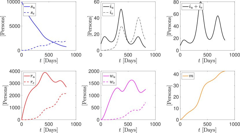
Figure 2: Simulation results with the model (5)-(13) with the parameters found in Table 2. With constant parameter values, the model is able to reproduce the qualitative behavior of the COVID-19 pandemic.

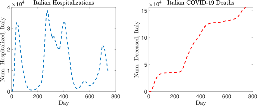
Figure 3: Number of hospitalized persons (left) and deaths (right) in Italy. We see that, when compared to Fig. 2, many of the key features are preserved: the qualitative behavior of the infection and deceased curves show a good resemblance with the observed behavior of the COVID-19 pandemic.

4 Conclusions and Perspectives

In this brief note, we have introduced an SIRW2 model, related to the models shown in [10, 15]. The proposed model is intended to describe a more sophisticated immune-system process than that found in most models: by the incorporation of immune boosting, and by stratification in terms of persons with and without previous exposure to the disease (either by vaccination or prior infection). We then demonstrated, through proof-of-concept simulations, that this modeling immunity may naturally recreate wave-like behaviors. This is consistent with the long-term results of COVID-19 outbreak, without requiring time-dependent parameter adjustment. Qualitatively, we obtain good agreement with observed COVID-19 infection dynamics, providing strong evidence that, after a full parameter-fitting process, the proposed model may be well-suited for COVID-19, as well as other infectious diseases showing a similar behavior. Much work has to be done for further developments. In particular, the theory of the model must be further developed, including the analysis of a suitable definition of $R_{0}$ and $R_{t}$, stability and equilibrium solutions, and bifurcation analyses. Rigorous derivations describing the model behavior (for instance, the oscillation period) in terms of the model parameters is also important. Most importantly, an application of the model on real-world data, incorporating a rigorous parameter fitting process, is necessary as a quantitative validation. Finally, this modeling framework can of course be developed even further via the incorporation of additional factors, such as time-lags, hospitalizations, differentiation between symptomatic and asymptomatic infections, and other important epidemiological considerations.

References

- [1] Protezione Civile Italiana. Covid-19. https://github.com/pcm-dpc/COVID-19, 2020.
- [2] William Ogilvy Kermack and Anderson G McKendrick. A contribution to the mathematical theory of epidemics. Proceedings of the royal society of london. Series A, Containing papers of a mathematical and physical character, 115(772):700–721, 1927.
- [3] Dimitri Breda, Odo Diekmann, WF De Graaf, A Pugliese, and R Vermiglio. On the formulation of epidemic models (an appraisal of Kermack and McKendrick). Journal of biological dynamics, 6(sup2):103–117, 2012.
- [4] Herbert W Hethcote. The mathematics of infectious diseases. SIAM review, 42(4):599–653, 2000.
- [5] Alex Viguerie, Guillermo Lorenzo, Ferdinando Auricchio, Davide Baroli, Thomas JR Hughes, Alessia Patton, Alessandro Reali, Thomas E Yankeelov, and Alessandro Veneziani. Simulating the spread of COVID-19 via a spatially-resolved susceptible–exposed–infected–recovered–deceased (SEIRD) model with heterogeneous diffusion. Applied Mathematics Letters, 111:106617, 2021.
- [6] Malú Grave, Alex Viguerie, Gabriel F Barros, Alessandro Reali, and Alvaro LGA Coutinho. Assessing the spatio-temporal spread of COVID-19 via compartmental models with diffusion in Italy, USA, and Brazil. Archives of Computational Methods in Engineering, 28(6):4205–4223, 2021.
- [7] Sheng Zhang, Joan Ponce, Zhen Zhang, Guang Lin, and George Karniadakis. An integrated framework for building trustworthy data-driven epidemiological models: Application to the COVID-19 outbreak in New York City. PLoS computational biology, 17(9):e1009334, 2021.
- [8] Nicola Parolini, Luca Dede’, Paola F Antonietti, Giovanni Ardenghi, Andrea Manzoni, Edie Miglio, Andrea Pugliese, Marco Verani, and Alfio Quarteroni. Suihter: A new mathematical model for COVID-19. application to the analysis of the second epidemic outbreak in Italy. Proceedings of the Royal Society A, 477(2253):20210027, 2021.
- [9] Mohamed Aziz Bhouri, Francisco Sahli Costabal, Hanwen Wang, Kevin Linka, Mathias Peirlinck, Ellen Kuhl, and Paris Perdikaris. COVID-19 dynamics across the US: A deep learning study of human mobility and social behavior. Computer Methods in Applied Mechanics and Engineering, 382:113891, 2021.
- [10] Hildeberto Jardón-Kojakhmetov, Christian Kuehn, Andrea Pugliese, and Mattia Sensi. A geometric analysis of the SIS, SIRS and SIRWS epidemiological models. Nonlinear Analysis: Real World Applications, 58:103220, 2021.
- [11] Nursanti Anggriani, Meksianis Z Ndii, Rika Amelia, Wahyu Suryaningrat, and Mochammad Andhika Aji Pratama. A mathematical COVID-19 model considering asymptomatic and symptomatic classes with waning immunity. Alexandria Engineering Journal, 61(1):113–124, 2022.
- [12] Thomas Crellen, Li Pi, Emma L Davis, Timothy M Pollington, Tim CD Lucas, Diepreye Ayabina, Anna Borlase, Jaspreet Toor, Kiesha Prem, Graham F Medley, et al. Dynamics of SARS-CoV-2 with waning immunity in the UK population. Philosophical transactions of the royal society b, 376(1829):20200274, 2021.
- [13] Daniel M Altmann and Rosemary J Boyton. Waning immunity to SARS-CoV-2: implications for vaccine booster strategies. The Lancet Respiratory Medicine, 9(12):1356–1358, 2021.
- [14] Elie Dolgin et al. COVID vaccine immunity is waning-how much does that matter. Nature, 597(7878):606–607, 2021.
- [15] Michiel van Boven, Hester E de Melker, Joop FP Schellekens, and Mirjam Kretzschmar. Waning immunity and sub-clinical infection in an epidemic model: implications for pertussis in The Netherlands. Mathematical Biosciences, 164(2):161–182, 2000.
- [16] Brian J Laidlaw and Ali H Ellebedy. The germinal centre B cell response to SARS-CoV-2. Nature Reviews Immunology, 22(1):7–18, 2022.
- [17] MATLAB. version R2019b. The MathWorks Inc., Natick, Massachusetts, 2019.