Bare Collapse, Formation of Neutron Star Binaries and Fast Optical Transients

Abstract

“Bare collapse", the collapse of a bare stellar core to a neutron star with a very small mass ejection links two seemingly unrelated phenomena: the formation of binary neutron star (BNS) systems and the observations of fast and luminous optical transients. We carried out calculations of the collapse due to electron-capture of both evolutionary and synthetic isentropic bare stellar cores. We find that the collapse results in the formation of a light $\sim 1.3\textup{M}_{\odot}$ neutron star and an ejection of $\sim 0.1\textup{M}_{\odot}$ at $\sim 0.1c$. The outer shell of the ejecta is composed of ⁵⁶Ni that can power an ultra-stripped supernova. The models we explored can explain most of the observed fast optical flares but not the brightest ones. Collapse of cores surrounded by somewhat more massive envelopes can produce larger amounts of ⁵⁶Ni and explain brighter flares. Alternatively, those events can arise due to interaction of the very energetic ejecta with winds that were ejected from the progenitor a few days before the collapse.

1 Introduction

Numerous evidence accumulated over the years for the existence of two channels for neutron star (NS) formation (Podsiadlowski et al., 2004; Piran & Shaviv, 2005; van den Heuvel, 2007, 2011; Beniamini & Piran, 2016; Tauris et al., 2017). The main channel involves the collapse of a massive star whose envelope is ejected in a powerful supernova (SN). If more than half of the mass of a binary system is ejected during the SN of the secondary, as would be the case in the SN of a massive star with a NS companion, the binary will be disrupted unless the collapse involves a kick in the right direction. The resulting binary systems will have a large eccentricity and a significant proper motion. However, two thirds of BNS systems have low eccentricity and small proper motion (Beniamini & Piran, 2016). This requires a second formation channel that operates in the majority of BNS systems. In this channel, the second neutron star forms without a significant mass ejection and with no kick, e.g. via an electron-capture SNe (Podsiadlowski et al., 2004). We refer to this channel as “bare collapse".

The discovery of the binary pulsar system PSR J0737-3039 (Burgay et al., 2003; Lyne et al., 2004) confirmed this picture (Piran & Shaviv, 2005). The orbital parameters of the system (small separation, low eccentricity and location in the Galactic plane) implied that the pulsar J0737-3039B had a very small $m<1.4-1.5\textup{M}_{\odot}$ progenitor and it was born with very little, $<0.1\textup{M}_{\odot}$, mass ejection and with no kick. Observations of the predicted very small proper motion, $10$ km/sec (Kramer et al., 2006; Deller et al., 2009), confirmed this scenario. The rate of these events, as inferred from the fraction of binary pulsars from the total number of pulsars suggests that bare collapses require unique progenitors (occurring for example in a very narrow mass range or specific metallicity) or unique process taking place during the binary evolution prior to the collapse (Tauris et al., 2017).

The very small mass ejection inferred in particular in PSR 0737-3039, but also indirectly in the majority of Galactic binary pulsars, suggests that these events can lead to fast optical transients powered by ⁵⁶Ni radioactive decay. For large brightness and short duration, the requirements are that a sufficiently large fraction of the ejected mass is ⁵⁶Ni and that the ejection velocity is large enough. Such fast optical transients (see e.g. Drout et al., 2014; Arcavi et al., 2016; Pursiainen et al., 2018) are characterised by a fast rise time of a few days and a peak luminosity comparable but typically somewhat lower than regular SNe. The fast rise time limits the mass ejection involved and in many cases the inferred mass is smaller than the amount of ⁵⁶Ni needed to explain the luminosity (Arcavi et al., 2016). However, these estimates assume a regular SN behavior. Bare collapses ejecta might be different.

In this work we simulate the collapse of a bare stellar core for both evolutionary (Jones et al., 2013; Tauris et al., 2015) and isentropic initial conditions. We use a modified version of the hydrodynamics code Vulcan (Livne, 1993), that includes both nuclear reaction chain and neutrino transport. We show that these bare collapse produces neutron stars while causing low mass ejection, hence consistent with the formation channel of most BNS systems. We focus on calculations of the ejected mass and its composition and velocity. Using these results we estimate the optical transient that arises from the ⁵⁶Ni  decay within this ejecta. The paper is structured as follows. We begin with a review of previous work in §2. This work is divided to two groups. The first deals mostly with the collapse and the subsequent mass ejection while the second deals with the nucleosynthesis and the resulting ultra-stripped SN light curve. We continue in §3 with a description of our methods. In §4 we present our results concerning the collapse and the nucleosynthesis within the ejecta. In §5 we describe the resulting optical transient and compare it to observations. We discuss the results in §6. We conclude and summarize in §7. In Appendix A we discuss the effect of neutrinos.

2 A brief sumamry of earlier work

Electron capture supernova (ECSN) takes place when electron capture, i.e. $e+p\to n+\nu_{e}$, reduce the electron degeneracy pressure in a O-Ne-Mg degenerate core of a massive star leading to collapse. In accretion induced collapse (AIC), a white dwarf (WD) accretes mass from a companion star, until it reaches the Chandrasekhar mass and collapses. Depending on details of the progenitor, AIC results in either a neutron star and a possible ejection of a small fraction of the star’s mass, or in a type Ia supernova.

From a computational point of view, but not from an astrophysical one, the ECSN of a bare core in which almost all the stellar envelope was lost via winds or due to interaction with a companion prior to the collapse, is very similar to AIC (when it does not result in a type Ia SN). In both cases, a progenitor of approximately Chandrasekhar mass collapses, and once the collapse begins the triggering mechanism is forgotten and the collapse is driven by electron capture at the center. The questions concerned with bare collapse deal both with the nature of the progenitor and the collapse process itself. We divide the discussion accordingly.

2.1 Progenitor models

Determination the progenitors for bare collapse is a complicated stellar evolution issue. The critical phase occurs at the very last stages of the stars’ lifetimes that are evolving at extreme speed. We don’t address this question in this work and we use evolutionary initial configurations by Jones et al. (2013); Tauris et al. (2015) as well as isentropic progenitor models.

Nomoto (1984, 1987), evolved helium cores of massive stars in the range of $\sim 8$-$10\textup{M}_{\odot}$. In all cases, an O-Ne-Mg core was formed. In the $M_{\mathrm{tot}}=10.4\textup{M}_{\odot}$ case, the core exceeded the critical mass for neon ignition ($1.37\textup{M}_{\odot}$). However, in the lighter cases, the cores did not reach neon ignition. Instead, electron capture took place and the systems ended up in ECSNe.

Jones et al. (2013) revisited the evolution of $8$-$10\textup{M}_{\odot}$ stars. They evolved stars with initial mass $8.2,8.7,8.75,8.8,9.5,12\textup{M}_{\odot}$. Their calculations showed that the $8.2\textup{M}_{\odot}$ star evolved into a stable O-Ne-Mg WD, while the $9.5\textup{M}_{\odot}$ and $12\textup{M}_{\odot}$ stars ended their lives in type II Fe core collapse supernovae (CCSNe). It was unclear if the $8.7\textup{M}_{\odot}$ star evolved into a stable WD or induced an ECSN. However, the $8.75\textup{M}_{\odot}$ and $8.8\textup{M}_{\odot}$ stars ended as stripped bare O-Ne-Mg cores and collapsed in ECSN. These results suggest that the promising range of single star progenitors for stripped ECSNe is narrow, with initial mass $8.7\textup{M}_{\odot}\leq M\leq 9.5\textup{M}_{\odot}$

Tauris et al. (2015) presented a systematic investigation of the progenitor evolution leading to ultra-stripped supernovae, i.e. SNe whose progenitors are stellar cores with extremely low helium envelope mass $<0.2\textup{M}_{\odot}$. Progenitors of this kind can exist in close binaries in which tidal stripping by the companion star alters the evolution significantly (see e.g. Podsiadlowski et al., 2004). The initial masses of the stars considered by Tauris et al. (2015) are, therefore, significantly smaller than the initial masses discussed for single stars. Tauris et al. (2015) evolved systems of a $2.5$-$3.5\textup{M}_{\odot}$ He-star with a $1.35\textup{M}_{\odot}$ NS companion, with different orbit periods. They found that ECSN only occurred in a limited range of progenitor mass, $M_{\mathrm{He}}=2.60$-$2.95\textup{M}_{\odot}$, depending on the orbit’s period.

2.2 Collapse simulations

The collapse of Chandrasekhar mass degenerate cores was calculated earlier mostly in the context of AIC. However, from a computational point of view, AIC is similar to our scenario. Woosley & Baron (1992) considered a progenitor of C-O white dwarf of initial mass $1.1\textup{M}_{\odot}$ which was obtained from Nomoto Nomoto (1986). The WD slowly accreted mass up to approximately the Chandrasekhar limit and then collapsed. The calculations didn’t reach a very late stage in the simulation, hence, they found only a tiny amount of ejected mass ($\approx 10^{-4}\textup{M}_{\odot}$) during the prompt phase of the collapse, but they estimated that the neutrino-driven wind will eject about $0.01\textup{M}_{\odot}$.

Using the same progenitor, Fryer et al. (1999) found later mass ejection of $0.1$-$0.3\textup{M}_{\odot}$ under various assumptions on input physics: equation of state (EOS), neutrino physics and relativistic effects. They found that apart from the EOS, non of the parameters significantly changed the amount of ejected mass, that varied by factors of at most $3$. As for the effects of the EOS, they showed that changes in the EOS explain the difference between their results (as well as other similar results such as those of Hillebrandt et al. (1984) and Mayle & Wilson (1988)) of $\sim 0.1\textup{M}_{\odot}$ mass ejection, and the results of Woosley & Baron (1992) which used the same progenitor but failed to eject a significant amount of mass by the shock mechanism

Most recently, Sharon & Kushnir (2020) used a modified version of the Vulcan 1D code Livne (1993) to calculate AIC, of a synthetic Chandrasekhar-mass star, with an isentropic core in a hydrostatic equilibrium, focusing on an accurate treatment of the EOS. They found an ejected mass of a few $\times 10^{-2}\textup{M}_{\odot}$ with an outflow velocity of $0.15$-$0.3c$, and the ejecta was composed mainly of ⁵⁶Ni . With no neutrino transport the initial $Y_{e}=0.5$ was kept throughout their calculations, and as we will see later this results in all the ejecta being ⁵⁶Ni .

As we focus on mass ejection it is worth noting that these earlier studies revealed three main mechanisms for mass ejection in ECSN and AIC (Fryer et al., 1999). First, in the prompt mechanism, the converging collapse shock bounces off the core, and the resulting diverging shock ejects the outer shells. Second, in the delayed-neutrino mechanism, the bounced shock initially stalls. However, after $20$- $200$ms, the shock revives due to neutrino heating and drives mass ejection. Lastly, in the neutrino driven wind mechanism, neutrino emission by the the newly formed hot proto-neutron star is absorbed in the outer (less dense) layers of the star, causing mass ejection.

2.3 Nucleosynthesis and light curve calculations

A different route to understanding ultra-stripped SNe is to investigate the long-term expansion of the ejecta and compute the resulting light curve. Such works do not follow the dynamics of the progenitor through its collapse. Instead, in such works a large amount of energy is injected to the outer shell of the progenitor, which then drives the mass ejection. The detailed nucleosynthesis and the light curve are computed in post-processing methods after the hydrodynamic calculation. This method is often referred to as explosive nucleosynthesis simulations.

Moriya et al. (2017) have used this method to compute the nucleosynthesis and light curve by the collapse of an ultra-stripped progenitor computed by Tauris et al. (2013). The progenitor was initially a $2.9\textup{M}_{\odot}$ He star, evolved as a binary of a $1.35\textup{M}_{\odot}$ NS. Moriya et al. (2017) found that ⁵⁶Ni of mass $\approx 0.03\textup{M}_{\odot}$ was formed in the ejecta, and that the rise time of the bolometric light curve was $5$-$10$ days. The progenitor they used is similar to one of the progenitors we use by Tauris et al. (2015).

Most recently, Sawada et al. (2021) have performed explosive nucleosynthesis simulations of C-O progenitors of core mass $1.45$-$2\textup{M}_{\odot}$ computed by Suwa et al. (2015). For the lighter progenitors, they found that $0.01$-$0.02\textup{M}_{\odot}$ of ⁵⁶Ni was synthesized in the ejecta, and the light curves had rise times of a few days.

3 Methods

3.1 The overall scheme

We use the Vulcan code (Livne, 1993), with some modifications, to carry out one-dimensional simulations, including hydrodynamics, neutrino transport and nuclear burning. The hydrodynamics is non-relativistic, and its scheme is explicit and Lagrangian. We used an adaptive mesh refinement (AMR) mechanism to allow a dynamical refinement of the mesh in the important regions. AMR was mainly used to decrease the resolution of the newly formed NS after bounce, and to increase the resolution in the ejected mass at late times. The initial grid in our standard simulations consists of 2842 cells, about half of them describe the inner $\sim 1.2\textup{M}_{\odot}$ which eventually remains bound, and the remaining cells describe the outer envelop. In this initial grid, the cell mass was equal to $10^{-3}\textup{M}_{\odot}$ for most of the star, where the cells at the outer region of the progenitor were increasingly smaller in mass, as low as $5\times 10^{-5}\textup{M}_{\odot}$. At later times, once the PNS has formed and no longer affects the ejecta, we gradually reduce the resolution of it to $\sim 100$ cells. We checked convergence by reducing the resolution with respect to two main parameters, first increasing the size of the numerical cells in the initial grid, and secondly increasing the maximal allowed size of a numerical cell in the AMR mechanism. Reducing the resolution by a factor of few with respect to these parameters did not change our qualitative results. For the isentropic progenitor (see §4.1), in either resolution a PNS was formed, with ejection of $\sim 0.1\textup{M}_{\odot}$, with similar composition. Quantitatively, the results varied by up to $10$-$20$%.

3.2 The Equation of state

The densities in the collapse vary from $\sim 10^{5}{\mathrm{g}}~{}{\mathrm{cm}^{-3}}$ to $\gtrsim 10^{14}{\mathrm{g}}~{}{\mathrm{cm}^{-3}}$. We use two different EOSs for the different thermodynamical regimes. For high densities, namely the part of the progenitor which eventually results as part of the NS, we use a tabulated EOS for nuclear material. The EOS is based on tables originally provided by Shen et al. (1998a, b) . The EOS table (compiled by O’Connor & Ott (2010)) utilizes the relativistic mean field (RMF) theory, and calculates the EOS for homogeneous nuclear matter, as well as for inhomogeneous matter using the Thomas-Fermi approximation. The matter is assumed to be in NSE, and to be comprised of a mixture of neutrons, protons, alpha-particles, a single species of heavy nuclei, and leptons. For the lower densities, namely the part of the progenitor which is later ejected, we use the EOS of degenerate electrons gas with free ions.

3.3 Neutrino transport

The neutrino transport scheme (based on an unpublished work of Eli Livne) solves the transport equation implicitly in the co-moving frame, adequately treating transparent regions and opaque ones. The scheme is inherently built to approach the diffusion method for opaque regions, and the discrete-ordinates method $S_{n}$ for transparent regions. For the $S_{n}$ method, we usually used $5$ azimuthal partitions, i.e.  $n=5$, but we checked $n>5$ as well and found no significant differences in the results. The neutrinos cross-sections were taken from Burrows et al. (2006). We used $18$ energy groups for the neutrinos, with the bin cetners between $0.5$-$286.3$ MeV, with a logarithmic spacing of the size of the energy bins. The size of the $k$’th energy bin is $\approx 1.29^{k-1}$ MeV.

In our simulations, we considered only $\nu_{e}$ and $\bar{\nu}_{e}$. We estimate that the effect of the $\nu_{\nu}$ and $\nu_{\tau}$ flavors to be insignificant for the results we are interested in. These neutrinos are not involved in nuclear interactions that change the electron fraction. Furthermore, their absorption cross sections are weaker, reducing their impact on the ejecta. We expect that the main effect of these neutrinos would be enhancing the cooling rate in the late phase of the process, once the neutron star forms.

3.4 Nuclear chain

Nuclear burning was calculated using reactions rates based on Rauscher & Thielemann (2000, 2001) with a network of $54$ isotopes. We validated the nuclear burning results using SkyNet (Lippuner & Roberts, 2017) as discussed in §4.1.1.

3.5 The progenitors

Numerous possible progenitors may evolve in different stellar evolution environments, during the last period of star’s lifetime as discussed in §2.1. We do not solve this question here, but rather consider two different types of progenitors, namely synthetic isentropic progenitors, and evolutionary progenitors obtained from detailed stellar evolution studies. We show that the results for both types are similar. This allows us to use the isentropic progenitors as a generic model.

Our first type of progenitor is isentropic Chandrasekhar-mass white dwarfs in hydrostatic equilibrium. For our standard simulations we used a progenitor with a central density of $2.2\times 10^{10}{\mathrm{g}}~{}{\mathrm{cm}^{-3}}$ and a central temperature of $1.8\times 10^{9}\mathrm{K}$. Fig. 1 shows the thermodynamic properties of the progenitor.

A second progenitor was evolved by Jones et al. (2013) from He core of a $8.75\textup{M}_{\odot}$ star (see §2.1). It is a degenerate core of mass $1.37\textup{M}_{\odot}$, most of it composed mainly of ¹⁶O and ²⁰Ne, where the outer $0.02\textup{M}_{\odot}$ is composed mainly of ¹²C with some ¹⁶O, ²⁰Ne and ²⁴Mg. Fig. 1 shows the initial profile. It has a central density of $2.27\times 10^{10}{\mathrm{g}}~{}{\mathrm{cm}^{-3}}$ and a central temperature of $1.75\times 10^{9}\mathrm{K}$, similar to our standard isentropic star. At its initial state, the progenitor is at the onset of collapse after electron capture has very mildly started at its center. The initial electron fraction of the progenitor is slightly smaller than $0.5$ for most of the star. The material has small inwards velocities, but the kinetic energy is negligible compared to the gravitational energy of the resulting NS. As a test, we performed minor adjustments to the initial profile so it would be in hydrostatic equilibrium. The results of the collapse of this adjusted profile were very similar to the results of the original profile, and we do not discuss it further in this work.

We also consider a third progenitor calculated by Tauris et al. (2015). This progenitor arises as a result of a binary evolution, as discussed in §2.1. It is considerably less dense compared to the other progenitors we examined, with the central density lower by a factor of $\sim 100$ than the central density of the progenitor found by Jones et al. (2013) for the single evolution. Figure 1 shows the density and temperature profiles of the main three progenitors we used in this work.

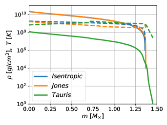
Figure 1: Initial density (full lines) and temperature (dashed lines) for the isentropic progenitor (blue), and for the evolutionary progenitors of Jones et al. (2013) (orange) and Tauris et al. (2015) (green). The density profiles for the isentropic progenitor and for the progenitor of Jones et al. (2013) are almost identical.

4 Results

4.1 Isentropic progenitor

We discuss the main results of our simulation for the isentropic progenitor. The star is initially in hydrostatic equilibrium. As electron captures occurs spontaneously at the center, a region of low $Y_{e}$ expands from the center of the star outwards, and the value of $Y_{e}$ decreases in time as electron capture keeps occurring. This causes an instantaneous reduction of the pressure due to the removal of degenerate electrons. This process continues and induces the collapse of material towards the center of the star. Eventually, material bounces back from the center as nuclear densities are achieved, launching a diverging shock wave that ejects the outermost layers.

Fig. 2 depicts mass elements trajectories as a function of time. We see that the star starts its collapse immediately. At $t\approx 0.12$ sec the bounce occurs and the diverging shock wave forms. Shock breakout occurs at $t\approx 0.2$ sec and the outermost layer of the star is ejected. The remnant is a compact star of mass $\approx 1.24\textup{M}_{\odot}$ which is initially at radius $\approx 40$ km. It is a proto-neutron star (PNS) which is still very hot, and so has a rather large radius. It takes for the PNS tens of seconds to achieve a standard NS radius, and we will discuss the late time evolution of the PNS in §4.1.2.

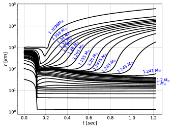
Figure 2: Trajectories of mass elements for the isentropic progenitor. Bounce and shock breakout occur at $t\approx 0.12$ sec and $t\approx 0.2$ sec, respectively. Approximately $0.08-0.1\textup{M}_{\odot}$ is ejected off the star immediately, and additional $0.02-0.04\textup{M}_{\odot}$ is ejected over $\approx 1\mathrm{\ sec}$.

4.1.1 The ejected mass

About $0.08-0.1\textup{M}_{\odot}$ is ejected immediately due to the shock, at $t\approx 0.2$ sec. Later on, a smaller amount of $0.02-0.04\textup{M}_{\odot}$ is ejected over a period of $\approx 1$ sec in a decreasing rate. We attribute this ejection to neutrino absorption and the neutrino driven wind mechanism. Fig. 3 shows the velocity profiles of the ejected mass at different times. We see that the ejected mass accelerates up to time $\approx 0.7$ sec, and then expands homologously. Most of the ejected mass travels at a small range of velocities, starting from $1.5\times 10^{9}{\mathrm{cm}}~{}{\mathrm{sec}^{-1}}$ at the inner regions of the ejecta, up to $3\times 10^{9}{\mathrm{cm}}~{}{\mathrm{sec}^{-1}}$ for the outermost regions. A tiny amount of mass (about $10^{-3}\textup{M}_{\odot}$) expands at up to about $7\times 10^{9}{\mathrm{cm}}~{}{\mathrm{sec}^{-1}}$.

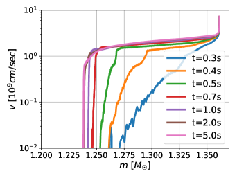
Figure 3: Velocity vs mass coordinate at different times. The ejecta accelerates during the first $\approx 0.7$ sec and then expands homologously, with velocities between $0.05c$ and $0.1c$ for most of the ejecta.

The ejecta contains at the time of shock breakout, $t\approx 0.2$ sec, only neutrons, protons and alpha particles. The temperatures behind the shock, at this time, are between $\approx 3$ MeV for the inner parts of the ejecta and $\approx 1$ MeV for the outer parts. The temperatures are so high that nuclei heavier than ⁴He disintegrate. The densities of the inner regions of the ejecta are at this time, a few times $10^{10}{\mathrm{gr}}~{}{\mathrm{cm}^{-3}}$, and these regions are comprised mostly of neutrons. Upon shock breakout, the material expands and cools. Starting from the outermost layer, and proceeding inwards as time progresses, heavier elements, in particular ${}^{56}\mathrm{Ni}$, form as the ejecta expands and so its density and temperature decrease. This stage occurs at densities of $\sim 10^{7}\mathrm{g}/\mathrm{cm}^{3}$ and temperatures of $\sim 0.5$ MeV, slightly larger for the inner ejecta compared to the outer ejecta. For each mass element, the burning phase is very short. The composition freezes out once the temperature and density drop slightly below this range.

At $t\approx 0.6$ sec the composition of all of the ejecta freezes. The outer $\approx 0.02\textup{M}_{\odot}$ of the ejecta has $Y_{e}\approx 0.5$ (see Fig. 4). This region has much lower density than the rest of the ejecta. Therefore, electron capture is substantially lower and $Y_{e}$ does not change from its initial $0.5$ value. ⁵⁶Ni is the most abundant isotope in NSE composition of relatively dense matter with $Y_{e}=0.5$ (partially because its nucleus has the same number of protons and neutrons). Hence ⁵⁶Ni forms in this outermost region. ⁵⁶Ni was created only at this very outer shell of the ejecta, which has important observational implications (see §5). The total ⁵⁶Ni mass was $\approx 0.02\textup{M}_{\odot}$. The composition of the ejected mass is shown in Fig. 5, where we focus on the outermost part of the ejecta, which is the region that ⁵⁶Ni was formed at and that was validated using SkyNet (see later). In a small inner shell we see a peak of ⁵⁸Ni. The rest of the ejecta, which is most of it, has $Y_{e}\approx 0.4$ (see Figure 4). In our Vulcan simulations ⁵⁶Fe is created in this low $Y_{e}$ region, but detailed nucleosynthesis calculations using SkyNet (see later) show that the composition in this region is more complicated and comprises of many iron group isotopes.

Vulcan employs a rather large network of 54 isotopes. However, it is clearly somewhat limited. We validated the Vulcan results using SkyNet  (Lippuner & Roberts, 2017), which includes 7836 isotopes and about 93000 reactions. We used the thermodynamic trajectories of different mass elements from the Vulcan simulation as an input to SkyNet, which solved the nuclear reaction equations. To account for the neutrino history of the mass elements, we assumed that the neutrinos were emitted at a time dependent rate from a source at the origin, as determined by the neutrino luminosity computed in our Vulcan simulations. The source is specified by a simplistic assumption of a Fermi-Dirac distribution with zero chemical potential, with an average energy of $k_{B}T_{\mathrm{source}}$, where the temperature determining the distribution was taken to be time dependent as well and is defined as follows. At the early stages after the collapse of up to $\lesssim 1$ sec, when the nucleosynthesis in the ejecta occurs, the PNS is qualitatively divided to two regions - an inner dense core of densities over $10^{14}{\mathrm{g}}/{\mathrm{cm}^{3}}$, and an outer envelope of much smaller densities that still accretes onto the PNS (see Figure 6). We assume that the inner dense core does not contribute to the neutrino flux at these early times as it is opaque, while the outer region is transparent. Therefore, we average the temperature only over the outer region with densities $<10^{14}{\mathrm{g}}/{\mathrm{cm}^{3}}$, and define the time dependent source temperature by $T_{\mathrm{source}}^{4}(t)=\int_{\mathrm{outer\ NS}}T^{4}(t,m)dm/\int_{\mathrm{outer\ NS}}dm$ with respect to the accumulating mass coordinate. This assumption mimics the presence of the remnant PNS, which is the source of neutrinos during the time that nucleosynthesis takes place.

We obtained an overall excellent match of $Y_{e}$ between our Vulcan simulation and the SkyNet simulation, as shown in Figure 4. Fig. 5 shows a comparison of the mass fraction of ⁵⁶Ni,⁵⁸Ni,⁴He and ⁵⁶Fe (the main isotopes that were obtained in the Vulcan simulations) in the outer $0.0225\textup{M}_{\odot}$ of the ejecta, as calculated by the Vulcan and the SkyNet simulations. SkyNet produces a similar composition in this outermost region, with ⁵⁶Ni being the dominant isotope, confirming Vulcan’s results. In both Vulcan and SkyNet simulations, the region with $Y_{e}\approx 0.5$ is precisely where ⁵⁶Ni is formed, and the two programs agree on the size of this region and its the composition, so correspondingly the total amount of ⁵⁶Ni in the ejecta is the same.

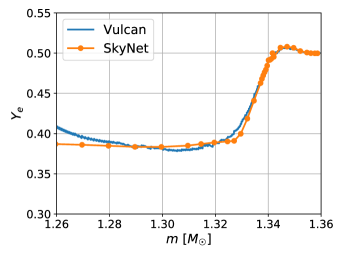
Figure 4: Electron fraction profile of the outer $0.1\textup{M}_{\odot}$ of the ejecta, by the Vulcan simulation (blue) and the SkyNet simulations (orange). The match is overall excellent, and the region of $Y_{e}\approx 0.5$ corresponds to the region where ⁵⁶Ni is formed.

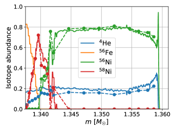
Figure 5: The abundance of ⁵⁶Ni,⁵⁸Ni,⁴He and ⁵⁶Fe for the outer $0.225\textup{M}_{\odot}$ of the ejecta, by our full Vulcan simulation (full lines) and by SkyNet (dashed lines). The results are almost identical for the ⁵⁶Ni,⁵⁸Ni and ⁴He abundance. ⁵⁶Fe that appears in the Vulcan results does not form in the SkyNet simulations in which the lower-$Y_{e}$ region comprises of many different iron peak isotopes that are not part of our standard Vulcan nuclear network.

4.1.2 The Neutron Star

The relevant time scale for the PNS to achieve equilibrium is much longer than the typical time scale for the ejection of the outer stellar layers or for the nucleosynthesis in the ejecta. To explore the later evolution as the PNS turns into a standard NS, we ran a longer simulation with two main changes. First, the ejecta was removed at $t=0.4$ sec. This is late enough for the dynamics of shock breakout and the mass ejection to have occurred, so the PNS and the ejecta are largely decoupled at this stage and we may focus only on the PNS. Second, the resolution was reduced to allow simulating long physical times with a reasonable run time. In this section we show results from our standard simulation up to $t=5$ sec, and from this modified simulation for $5<t\lesssim 30$ sec.

Figure 6 depicts the density and temperature profiles of the PNS for different times. The inner $\approx 0.7$-$0.8\textup{M}_{\odot}$ approaches nuclear density almost immediately. This critical point of $m\approx 0.8\textup{M}_{\odot}$ is where bounce occurred during the collapse at approximately $120$ msec. The outer part of the PNS is initially at densities lower by $1$-$2$ orders of magnitude. Even after $\sim 1$ sec there are still some dynamics at this region and matter keeps falling towards the PNS and its density increases. The temperatures range from $3$ MeV to $22$ MeV peaking at $m\approx 0.7\textup{M}_{\odot}$-$0.8\textup{M}_{\odot}$, where the bounce took place and where we saw a qualitative change in behaviour of the density profile. The temperatures keep increasing for a while as gravitational energy is released due to the contraction of the PNS that is turning into an ordinary NS.

The dynamics of the PNS keep going for a long period. The radius of the PNS, that was approximately $40$ km at $t\approx 1$ sec, decreases to $\lesssim 15$ km at the latest time of our simulation $t\approx 30$ sec, see Figure 7. The general picture at these late times, which we explain shortly, is similar to the known theory of PNS (see e.g. Burrows & Lattimer, 1986). Neutrinos escaping from the outer shells of the PNS reduce the neutrino radiation pressure and allow the outermost layers of the PNS to accrete on the inner PNS core. This causes the increase in temperature at early times. Next, the hot and opaque PNS heats inwards, while electron capture continuously reduces the electron fraction, until a hot NS is formed. Finally, after tens of seconds have passed, the hot NS cools down by neutrino emission and the NS becomes more compact. Note that our simulations included only $\nu_{e}$ and $\bar{\nu}_{e}$. Inclusion of the $\nu_{\mu}$ and $\nu_{\tau}$ flavors could accelerate the cooling process (but won’t change the qualitative behaviour).

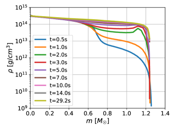
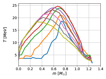
Figure 6: Density (top) and temperature (bottom) vs mass for the PNS, at different times. It takes a few seconds for the outer region ($\approx 0.5\textup{M}_{\odot}$) of the PNS to accrete and reach nuclear densities. At the first few seconds, the temperature increases as the PNS evolves and contracts. Then, the PNS heats from the middle towards the center, while cooling off its outer boundary. The profiles up to time $5$s were taken from our standard simulation. Later profiles were taken from a similar simulation tailored to allow simulating long physical times with a reasonable accuracy (see text).

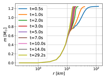
Figure 7: Accumulating mass vs radius, at different times. It takes many seconds for the PNS to reach an ordinary NS radius. The profiles at all times are taken from our lower-resolution simulation (see text), but the results are the same as in our standard simulation.

4.2 An evolutionary single-star progenitor

Next we simulated the collapse of an evolutionary progenitor calculated by Jones et al. (2013). The collapse of this progenitor resulted in the formation of a NS and a small amount of mass ejection, qualitatively and quantitatively very similar to the results discussed in §4.1. The velocity, mass, composition and electron fraction of the ejecta are very similar for both types of progenitors. This similarity is reassuring and shows the robustness of our key result, which is an ejected shell of $\approx 0.13\textup{M}_{\odot}$ traveling at $0.1c$, where the outer $0.02\textup{M}_{\odot}$ shell is composed of $77\%$ ⁵⁶Ni.

Trajectories of mass elements as a function of time are shown in Fig. 8. A remnant of $1.23\textup{M}_{\odot}$ is left. Approximately $0.14\textup{M}_{\odot}$ is ejected, most of it immediately after bounce. The ejecta eventually expands homologously with velocities of about $2$-$3\times 10^{9}{\mathrm{cm}}~{}{\mathrm{sec}^{-1}}$ (see Fig. 9). As in the case of the isentropic progenitor, a tiny amount of mass travels at much larger velocities.

The composition of the outermost region of the ejected mass at the final time of the simulation, long after it froze out, is shown in Fig. 10. As in the isentropic star case, we see an outer shell of $\approx 0.02\textup{M}_{\odot}$ which is composed mostly of ⁵⁶Ni, followed by a small shell of ⁵⁸Ni. Further in, there is a large bulk of ⁵⁶Fe, although, as discussed in §4.1.1, this ⁵⁶Fe bulk is in fact composed of various other iron group isotopes. As before, the outer shell in which the ⁵⁶Ni lies has an electron fraction $Y_{e}\approx 0.5$, while the main bulk has lower electron fractions $Y_{e}\approx 0.4$.

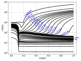
Figure 8: Trajectories of mass elements for the evolutionary single-star progenitor of Jones et al. (2013). Approximately $0.14\textup{M}_{\odot}$ is ejected due to the gravitational collapse, leaving a PNS of mass $1.23\textup{M}_{\odot}$. The results are very similar to the case of the isentropic progenitor.

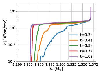
Figure 9: Velocity profiles of the outermost region of the ejecta at different times, for the evolutionary progenitor of Jones et al. (2013). The results are similar to those of the isentropic star.

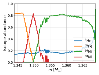
Figure 10: The final composition of the ejecta for the evolutionary progenitor of Jones et al. (2013). The results are similar to those of the isentropic star.

4.3 An evolutionary binary-star progenitor

We also simulated the collapse of a progenitor calculated by Tauris et al. (2015) which was evolved as a binary companion of a NS. This progenitor has a slightly larger mass of $\approx 1.45\textup{M}_{\odot}$ (including its tenuous envelope). In their work, Tauris et al. (2015) evolved the progenitor using the BEC code, which is usually suitable to follow the evolution only up to a few tens of years prior to the onset of gravitational collapse (Moriya et al., 2017). Continuing the evolution, using different codes, shows that the density of the progenitor increases significantly until it collapses (c.f. Müller et al. (2018)). Consequently, the initial configuration described in Tauris et al. (2015) is much larger and has a significantly lower density compared to the other cases we studied. Therefore, the rate of electron capture in the center of the star was not sufficient to induce its collapse in our simulations , when we used this initial configuration. Still, using this progenitor is interesting as it will demonstrate that our results are not very sensitive to the initial conditions assumed. To calculate the collapse, instead of continuing its evolution we simply induced the collapse by providing the progenitor with an inwards velocity, resulting in kinetic energy of $\sim 10^{50}$erg. We also managed to induce the collapse in a different simulation of this progenitor, by artificially reducing the value of $Y_{e}$ to $0.2$ for the inner $5\times 10^{-2}\textup{M}_{\odot}$ of the progenitor, at time $0$. The collapse took a little longer to occur in this case (bounce occurred at $t\approx 2.5$s), but the results were very similar. Trajectories of mass elements as a function of time are shown in Figure 11. Due to the large radius of this progenitor, the collapse occurs on a longer time scale and bounce is only at $t\approx 0.7$s. The outer $\approx 0.05\textup{M}_{\odot}$ of the star, which is a tenuous ${}^{4}\mathrm{He}$-${}^{12}\mathrm{C}$-${}^{16}\mathrm{O}$ envelope at a radius of $\sim 10^{5}$km, did not move significantly. Shock breakout did not occur during the entire simulation and is expected at time $\approx 10$sec. Once it occurs this outer region is expected to be ejected as well.

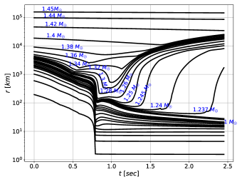
Figure 11: Trajectories of mass elements for the evolutionary binary-star progenitor of Tauris et al. (2015). The collapse was induced by providing the progenitor with an inwards velocity. A progenitor of mass $\approx 1.45\textup{M}_{\odot}$ collapses, and a PNS of mass $1.24\textup{M}_{\odot}$ is formed. The outer layers of the progenitor, as well as the tenuous envelope which did not move significantly during the collapse, are ejected. Shock breakout did not occur during the entire simulation and is expected at time $\approx 10$ sec. The results are similar to other progenitors we studied.

Still, despite all of these differences, the collapse resembles the cases studies in §4.1-§4.2. A NS of $\approx 1.24\textup{M}_{\odot}$ formed. The electron fraction is $Y_{e}\approx 0.5$ for the outer parts of the ejecta, and $Y_{e}\approx 0.4$ for the inner parts. At the final time of our simulation, the divergent shock is located at mass coordinate $m\approx 1.36\textup{M}_{\odot}$. Therefore, as shown in Figure 12, the composition at the outermost part is the original, ¹⁶O-²⁰Ne-²⁴Mg up to mass $\approx 1.39\textup{M}_{\odot}$, and ⁴He-¹²C-¹⁶O for the envelope. Below it there is a region which did go through nuclear burning but did not reach nickel. In the inner parts, the composition is similar to previous cases, with ⁵⁶Ni at the outer zones ($\approx 3\times 10^{-2}\textup{M}_{\odot}$ in this case), a narrow peak of ⁵⁶Ni, and then a some other iron peak elements where $Y_{e}\approx 0.4$ (see  §4.1.1). The velocities range between $1$-$2\times 10^{9}{\mathrm{cm}}/{\mathrm{sec}}$ for most of the ejecta. These are somewhat smaller, yet comparable to those found in the previous cases.

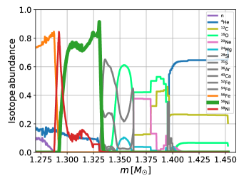
Figure 12: The composition of the ejecta vs the accumulating mass coordinate for the Tauris et al. (2015) progenitor. The divergent shock is located at mass coordinate $m\approx 1.36\textup{M}_{\odot}$, and so the outer region is at its initial composition. Below it there is a region which burnt partially and did not reach nickel. In the inner parts the composition is similar to previous cases, with ⁵⁶Ni at the outer zones ($\approx 3\times 10^{-2}\textup{M}_{\odot}$ in this case) and a narrow peak of ⁵⁸Ni (see  §4.1.1). The ⁵⁶Ni abundance is shown in a thick green curve.

We conclude that stars which evolve in binaries may also go through bare collapse and form a NS with similar mass, while ejecting mass with comparable properties, hence inducing a similar observed signal.

4.4 Different isentropic progenitors

We used the isentropic progenitor as a model to study the collapse of different stars, focusing on the effect of varying the progenitors’ mass.

We found that lighter progenitors with mass smaller than the Chandrasekhar mass by up to $\approx 0.1\textup{M}_{\odot}$ (with central density and temperature as in §3.5) may still collapse, with similar ejecta properties. In particular, this allows for the formation of even lighter NSs. On the other hand, light enough stars are stable and do not collapse nor produce NSs. The particular point of transition from stable to unstable WD (given accurate EOS, reaction rates and neutrino cross sections) is unclear and should be further investigated.

Turning to heavier progenitors, we considered progenitors of approximately Chandrasekhar mass, with an outer envelope added on top. These progenitors are the same as the original Chandrasekhar-mass isentropic progenitor up to some point which is approximately at $m_{0}\approx 1.35\textup{M}_{\odot}$, namely slightly below the original boundary. From this point, we add an outer uniform shell whose physical properties are the same as those of the mass element at $m_{0}$. To allow envelopes of different densities, we simply change $m_{0}$ by a small amount. Some examples of initial configurations of heavier progenitors are shown in Figure 13.

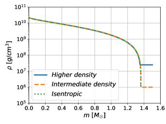
Figure 13: Initial density for two modified $1.5\textup{M}_{\odot}$ progenitors. One with a higher density envelope (blue) and another with an intermediate density envelope (orange), compared to the Chandrasekhar mass isentropic progenitor (green). The density is the same as the isentropic progenitor until some point, $m_{0}$, slightly below $1.35\textup{M}_{\odot}$. From this point, we add an outer uniform shell whose physical properties are the same as those of the mass element at $m_{0}$. To allow envelopes of different densities, we simply change $m_{0}$ by a small amount.

We note that adding the mass in this way can have significant and non trivial impact on the fate of the progenitor. For example instead of going through ECSN it may explode as a type Ia SN. We don’t consider these possibilities here. Instead, we only try to shed some light on the possible consequences of collapse of heavier progenitors assuming ECSN occurs in these initial conditions, without discussing the extent to which these conditions are valid to describe realistic more massive ECSN progenitors. As such these results should be taken with a grain of salt and clearly the question what is the structure of heavier progenitors should be explored more extensively. With all that being said, one possible realistic scenario for ECSNe of WDs with envelopes could rise from the merger of two WDs, as suggested by Lyutikov & Toonen (2019); Lyutikov (2022) (others may include the partial shedding of a heavier envelope in the pre-collapse evolution due two stellar wind or interaction with a binary). So although these simplified models are artificial from a stellar evolution point of view, they can give us indications on what happens in realistic configurations of this nature.

For progenitors with envelopes whose density is above a certain value, our simulations resulted in a collapse leading to similar ejecta properties, mass and composition, as in §4.1, independent of the mass. Specifically, for the particular case of $\rho_{env}\approx 10^{7}\frac{\mathrm{g}}{\mathrm{cm}^{3}}$, and envelope mass up to $0.25\textup{M}_{\odot}$, we found mass ejection of $0.11$-$0.14\textup{M}_{\odot}$, of which $2$-$3\times 10^{-2}\textup{M}_{\odot}$ was composed of ⁵⁶Ni , at ejecta velocities of $1$-$3\times 10^{9}{\mathrm{cm}}/{\mathrm{sec}}$. Trajectories of mass elements as a function of time, and the composition of the ejecta, for a $\approx 1.5\textup{M}_{\odot}$ progenitor, are shown in Fig. 14 and Fig 15 respectively. The resulting NS is, of course, correspondingly heavier. Fig. 16 shows that the NS mass increases linearly with the progenitor mass with slope approximately $1$. As the mean mass for NSs in BNS systems is $\approx 1.33\textup{M}_{\odot}$ (Özel & Freire, 2016), these calculations show that bare collapse is consistent with the formation of BNS systems in this regard as well.

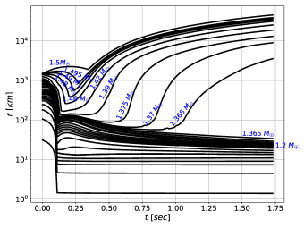
Figure 14: Trajectories of mass elements for a progenitor with a high density envelope, and total mass $\approx 1.5\textup{M}_{\odot}$. The progenitor undergoes collapse similar to previous cases, with $\approx 0.14\textup{M}_{\odot}$ ejected. This results in the formation of a $1.37\textup{M}_{\odot}$ NS, which is heavier compared to all cases studied in previous sections. There is a slight early expansion of the very outer mass element near the boundary of the progenitor, caused by the initial progenitor being out of hydrostatic equilibrium.

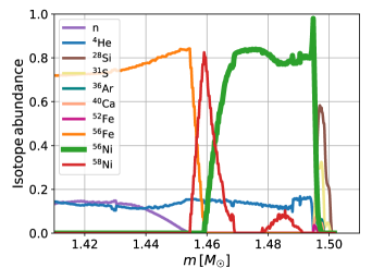
Figure 15: The final composition of the ejecta for a progenitor with a high density envelope, and total mass $\approx 1.5\textup{M}_{\odot}$. The ⁵⁶Ni mass, $\approx 3\times 10^{-2}\textup{M}_{\odot}$, and the composition are similar to those found in previous studied cases.

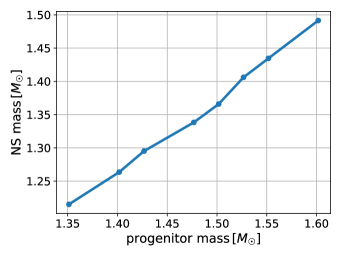
Figure 16: The remnant NS mass vs the progenitor mass. It is approximately linear with slope $1$, meaning that excess mass in the progenitor stays bound as part of the NS. This occurs for progenitors with dense enough envelopes.

In the other limit, where the envelope density is very small (in particular lying at large radii), the envelope does not affect the collapse or the resulting NS significantly. Instead, the envelope is simply ejected, without undergoing nuclear burning.

In the intermediate density regime, we were able to find cases where the envelope was on the one hand dense enough to collapse (and in particular reach the suitable thermodynamic state for nuclear burning), but on the other hand is light enough for most of the mass that was added to eventually be ejected upon the bounce. Figure 19 depicts the ⁵⁶Ni mass as a function of the progenitor mass, for the particular case of $\rho_{env}\approx 10^{6}{\mathrm{g}}/{\mathrm{cm}^{3}}$. It can be seen that about $1/2$ of the added mass is converted to ⁵⁶Ni . The largest progenitor we considered, with a mass of $1.66\textup{M}_{\odot}$, produces $16\times 10^{-2}\textup{M}_{\odot}$ of ⁵⁶Ni , $5$-$8$ times larger than the amount formed in the Chandrasekhar-mass progenitors. We also validated these nucleosynthesis results using SkyNet, by the method discussed in §4.1.1, and found an excellent agreement. For these progenitors, the mass of the formed PNS was $1.25$-$1.3\textup{M}_{\odot}$. Trajectories of mass elements as a function of time, and the composition of the ejecta, for a $\approx 1.5\textup{M}_{\odot}$ progenitor, are shown in Fig. 17 and Fig 18 respectively. The amount of ⁵⁶Ni formed in this particular intermediate density regime progenitors , $9\times 10^{-2}\textup{M}_{\odot}$, is considerably larger from all previous simulations of ECSNe. For instance, Sawada et al. (2021) argued that is difficult to achieve ⁵⁶Ni mass larger than $5\times 10^{-2}\textup{M}_{\odot}$. The particularly high amount of ⁵⁶Ni in our simulations may arise from the specific envelope density we have chosen (together with the simplified model of uniform envelope density). While such models may not describe correctly realistic ECSN progenitors, they still suggest that some unique progenitors could synthesize more ⁵⁶Ni than previously estimated.

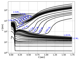
Figure 17: Trajectories of mass elements for a progenitor with an intermediate density envelope, and total mass $\approx 1.5\textup{M}_{\odot}$. The progenitor undergoes collapse similar to previous cases and result in the formation of a $1.29\textup{M}_{\odot}$ NS. Most of the additional envelope mass is ejected, yet some of it remains bound and the NS is slightly heavier compared to the cases studied in previous sections. In this intermediate density envelope density case, the ⁵⁶Ni mass is significantly larger.

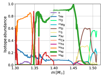
Figure 18: The final composition of the ejecta for a progenitor with an intermediate density envelope, and a total mass $\approx 1.5\textup{M}_{\odot}$. The ⁵⁶Ni mass is $\approx 9\times 10^{-2}\textup{M}_{\odot}$, significantly larger than previously studied cases. The nucleosynthesis results were also validated using SkyNet.

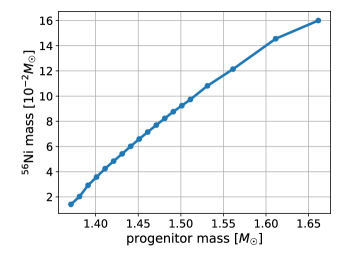
Figure 19: The ⁵⁶Ni mass in the ejecta vs the progenitor mass. About $1/2$ of the added mass is ejected as ⁵⁶Ni. The nucleosynthesis results were also validated using SkyNet. This occurs for progenitors with envelopes of a limited range of densities.

5 Observational Signature

5.1 Fast Transients

The gravitational collapse of bare degenerate cores results in many cases in the ejection of $\sim 0.1\textup{M}_{\odot}$, at about $0.1c$. The outermost layer of this ejecta is composed of $\sim 0.02\textup{M}_{\odot}$ of ⁵⁶Ni. The decay of this ⁵⁶Ni will produce an ultra-stripped SN with very different characteristic luminosity and rise time fro a typical SN. We turn now to consider the observational characteristics of such an outer thin shell of radioactive nickel, as it expands homologously. We use a simple model that gives an order of magnitude estimate of the observed bolometric luminosity, peak time and temperatures.

Consider a shell of mass $M$, radius $R$ and width $\Delta R$, that is moving homologously so that $R=vt$ and $\Delta R\propto t$. Let $M_{{}^{56}\mathrm{Ni}}$ be the mass of ⁵⁶Ni within the shell and $\kappa$ the opacity of the shell. The optical depth across the shell is given by

$$\tau=\int_{R-\Delta R}^{R}\kappa\rho dr\approx\frac{\kappa M}{4\pi(vt)^{2}}\ ,$$ (1)

where we have assumed that the opacity is constant, the density does not depend too strongly on $r$, and $\Delta R\ll R$. Since the ⁵⁶Ni is arranged in a thin shell this reduces $\tau$ by a factor of $3$, compared to a sphere.

Radiation escapes at time $t$ only from regions whose optical depth $\tau^{\prime}$ satisfies ${c}/{\tau^{\prime}}>v$. At early times, the effective observable mass is $M_{\mathrm{obs}}(t)={4\pi cvt^{2}}/{\kappa}$ and the bolometric light curve rises like $t^{2}$. The luminosity peaks when radiation can escape from the whole shell, namely at:

$$t_{\mathrm{peak}}=\sqrt{\frac{\kappa M}{4\pi cv}}\approx 0.5~{}{\rm days}~{}\frac{\kappa_{-1}^{1/2}M_{-2}^{1/2}}{v_{-1}^{1/2}}\ ,$$ (2)

where we use the notation $Q_{x}=Q/10^{x}$ in cgs units but masses are measured in $\textup{M}_{\odot}$, velocities in $c$ and time in days.

For $t_{\mathrm{peak}}\ll\tau_{{}^{56}\mathrm{Ni}}$ the peak luminosity is:

$$L_{\mathrm{peak}}\approx\frac{M_{{}^{56}\mathrm{Ni}}\epsilon_{{}^{56}\mathrm{Ni}}}{\tau_{{}^{56}\mathrm{Ni}}}\approx 7.7\times 10^{41}\times M_{{}^{56}\mathrm{Ni},-2}{\mathrm{erg}}/{\mathrm{s}}\ ,$$ (3)

where $\epsilon_{{}^{56}\mathrm{Ni}}\approx 2.96\times 10^{16}$ erg/g is the energy released per gram of decaying ⁵⁶Ni , $\tau_{{}^{56}\mathrm{Ni}}\approx 8.8$ day is the mean lifetime of ⁵⁶Ni , and $M_{{}^{56}\mathrm{Ni},-2}=M_{{}^{56}\mathrm{Ni}}/(10^{-2}\textup{M}_{\odot})$. The effective temperature,

$$T_{\mathrm{peak}}=\Big{(}\frac{L_{\mathrm{peak}}}{4\pi(vt_{\mathrm{peak}})^{2}\sigma}\Big{)}^{1/4}\approx 1.6\times 10^{4}~{}\kappa_{-1}^{-1/4}v_{-1}^{-1/4}\Big{(}\frac{M_{{}^{56}\mathrm{Ni}}}{M}\Big{)}^{1/4}\ K\ ,\$$ (4)

corresponds to a UV/blue signal. The spectrum will show lines according to the specific composition typical for bare collapse, which is mostly iron group and lighter elements. We expect that different bare collapses should have comparable spectra.

After the peak, the luminosity decreases due to a combination of the decrease in the amount of the decaying ⁵⁶Ni , and the leakage of the decay products out from the expanding system. The latter is more important, leading to a significantly faster decline than the one arising from the ⁵⁶Ni lifetime. We expect the whole system to be optically thin long before we can see the typical radioactive decay time of ⁵⁶Ni .

A typical value of $M_{{}^{56}\mathrm{Ni}}=0.02$-$0.03\textup{M}_{\odot}$ of ⁵⁶Ni is sufficient to explain a fast transient with a peak luminosity of $\approx 2\times 10^{42}{\mathrm{erg}}/{\mathrm{s}}$ or equivalently a peak absolute magnitude of $\approx-17$. The largest values of ⁵⁶Ni  that we have found of $\approx 0.16\textup{M}_{\odot}$ yields a peak absolute magnitude of $\mathcal{M}_{\mathrm{peak}}\approx-19$. The typical rise time of these events is 1-2 days.

Combining Eqs. (2) and (3) we obtain the ejecta velocity needed for a given rise time, and peak absolute magnitude:

$$v_{-1}=0.25\kappa_{-1}\frac{M_{-2}}{t_{\mathrm{peak},1}^{2}}\approx 3.2k_{-1}\frac{M}{M_{{}^{56}\mathrm{Ni}}}\frac{L_{\mathrm{peak},43}}{t_{\mathrm{peak},1}^{2}}\ .$$ (5)

The minimal required velocity to obtain a transient of given peak time $t_{\mathrm{peak}}$ and peak absolute magnitude $\mathcal{M}_{\mathrm{peak}}$ for a given $M_{{}^{56}\mathrm{Ni}}$ is shown in Fig. 20 , assuming $\kappa_{-1}=1$. This minimal velocity is obtained when $M=M_{{}^{56}\mathrm{Ni}}$. Also shown is the dependence of $\mathcal{M}_{\mathrm{peak}}$ on $t_{\mathrm{peak}}$ for different ⁵⁶Ni masses. Together, this outlines the region in which fast flares can be explained by bare collapses. These values can explain many of the fast transients and in particular most of the “golden sample" of Drout et al. (2014).

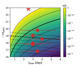
Figure 20: Contour map of the minimal required velocity for given peak time and peak absolute magnitude , obtained for a given outer shell of $M_{{}^{56}\mathrm{Ni}}$, namely $M=M_{{}^{56}\mathrm{Ni}}$ and $\kappa_{-1}=1$. The black curves (full lines) correspond to the values$v/c=0.001,0.003,0.01,0.03,0.1,0.3,1$. Each such curve defines the most luminous events theoretically possible by our model, for a given velocity $v$. The black dashed lines show the value of $\mathcal{M}_{\mathrm{peak}}$ for $M_{{}^{56}\mathrm{Ni}}=0.02,0.03,0.05,0.1,0.16,0.25\textup{M}_{\odot}$. The bold full curve corresponds to $v/c=0.1$ which is the typical velocity for most of the ejecta, and the bold dashed line corresponds to $M_{{}^{56}\mathrm{Ni}}=0.16\textup{M}_{\odot}$ which is the highest ⁵⁶Ni mass obtained in our simulations. Also shown in red are some of the PS1 fast transients (Drout et al., 2014, as circles) and AT 2018cow (as a star).

5.2 Other possible observational signatures

5.2.1 Very luminous fast transients

The luminosity arising from ⁵⁶Ni decay in bare collapses can explain many of the fast transients. For example it is sufficient to explain the “golden sample" discussed by Drout et al. (2014). However, it falls short of the brightest ones like AT 2018cow whose peak luminosity is $\sim 4\times 10^{44}$erg/s (Perley et al., 2019) or the brightest fast transients reported by (Drout et al., 2014) that would require more than $0.3\textup{M}_{\odot}$ of ⁵⁶Ni .

The ejecta of $\sim 0.1\textup{M}_{\odot}$ travelling at $\sim 0.1c$, has a significant kinetic energy of the order of $\sim 10^{51}$ erg. This is comparable to the kinetic energy of a typical (much more massive) SN. Tapping even a small fraction of this energy can lead to signal that explains the brightest transients. This could happen if on a time scale of a day or so, the ejecta collide with material in the proximity of up to $\approx 0.1$ light day from to the progenitor. Such material could be mass ejected from the progenitor just prior to the collapse. While we cannot demonstrate that such mass ejection takes place on this time scale, given the essential extensive mass loss of progenitors for bare collapse and the fast evolution during the last stages before the collapse, this is clearly possible. Assuming the material with which the ejecta collides had a velocity $v_{\mathrm{w}}$, it would have needed to escape the progenitor up to $\approx 10~{}[v_{\mathrm{w}}/({3000\mathrm{km/sec)}}]^{-1}$ days prior to the collapse.

If the mass of the ejecta, $\sim 0.1\textup{M}_{\odot}$, is smaller than the mass with which it collides, this collision could transfer a large fraction of the kinetic energy to thermal energy. This is about $100$-$1000$ times larger than the total energy released by the radioactive decay of the ⁵⁶Ni. This could easily power even the very rare brightest events. It is important to note that much smaller mass is needed for this scenario to happen, as compared to a similar situation with standard SNe which eject much more mass. Moreover, this scenario can fit nicely with the evolution of bare collapse progenitors which lose most of their envelope.

5.2.2 The Remnants

In the long run, bare collapse events produce a SN remnant (SNR) like signature. As the ejecta expands it sweeps up mass. Initially it is coasting at a constant velocity and as it accumulates more and more mass the luminosity increases like $t^{2}$. The Sedov-Taylor (ST) phase begins at

$$t_{\mathrm{ST}}=\big{(}\frac{3M_{\mathrm{ej}}}{4\pi\rho_{\mathrm{ISM}}v_{\mathrm{ej}}^{3}}\big{)}^{1/3}\approx 40~{}{\rm years}~{}~{}{M_{\mathrm{ej,-1}}^{1/3}{n_{\mathrm{ISM}}^{1/3}{v_{-1}}}}\ ,$$ (6)

where $n_{\mathrm{ISM}}$ is the interstellar medium (ISM) density. At this stage the ejecta have passed through a mass of ISM equal to $M_{\mathrm{ej}}$. The energy dissipation rate is maximal at $t_{\mathrm{ST}}$. As the mass of the ejecta is much lower than the mass of a SN ejecta and its velocity is faster, $t_{\mathrm{ST}}$ is shorter by about a factor of $\approx 10$, than in a regular SN. This implies that the peak bolometric luminosity of this bare-collapse SNR, $\approx 10^{42}$ erg/sec, is larger than the peak luminosity of a regular SNR by a similar factor. This luminosity is comparable to the peak luminosity of a rare SNR arising from a superluminous SN. Over even longer time scale the Sedov-Taylor phase continues and it will be impossible to distinguish this remnant from a regular SNR. In this phase all that matter is the total energy and the external density and the initial ejecta mass and velocity are not relevant.

6 Discussion

We have shown that the collapse of a bare stellar core of around Chandrasekhar mass, results in a light, $\approx 1.2$-$1.35\textup{M}_{\odot}$, neutron star and ejection of $\approx 0.1$-$0.2\textup{M}_{\odot}$ at $\approx 0.1$c. We considered two evolutionary configurations that were derived from stellar evolution simulations by Jones et al. (2013) and by Tauris et al. (2015). Similar results were obtained for an isentropic initial configuration of hot white dwarf, and even when a light envelope of $\leq 0.35\textup{M}_{\odot}$ was added to it.

Naturally this neutron star is rather light. This is consistent with the observation that the mean mass of the neutron stars in BNS systems is $\approx 1.33\textup{M}_{\odot}$ (Özel & Freire, 2016). With such a small mass ejected, a binary composed of this progenitor and a companion neutron star would remain bound with small eccentricity and small proper motion. The double pulsar PSR J0737-3039 is a prototype of a system that formed in this way (Piran & Shaviv, 2005). This is also consistent with the observations that BNS systems with lower eccentricity and lower CM motion, that are expected to form in this channel, involve lighter neutron stars (van den Heuvel, 2007, 2011).

The collapse ejects $\sim 0.1\textup{M}_{\odot}$ of iron group elements with an outer shell composed mostly of ⁵⁶Ni . This outermost region where ⁵⁶Ni was formed had $Y_{e}=0.5$, consistently with the equal number of protons and neutrons in this isotope. This radioactive ejecta results in fast transients for two reasons. First, the ejecta velocities are $\approx 2$-$3\times 10^{9}{\mathrm{cm}}~{}{\mathrm{sec}^{-1}}$. As the rise time of the light curve is proportional to ${v_{\mathrm{ej}}}^{-1/2}$, this leads to faster transients by a factor of $\approx\sqrt{3}$, as compared to traditional SNe with $v_{\mathrm{ej}}=10^{9}{\mathrm{cm}}~{}{\mathrm{sec}^{-1}}$ (see e.g. Arcavi et al., 2016). Second, the ⁵⁶Ni lays in a shell at the outermost layer of the ejecta. The rise time determined by the expansion of a shell, rather than a sphere, is faster by a factor of up to $\sqrt{3}$. Moreover, the rise time was found to depend on the ⁵⁶Ni mass, rather than the entire ejecta mass. Together these two factors combine to shorten the transients by a factor of $\approx 3$, for a given ⁵⁶Ni mass. For the particular ejecta we obtained in our simulations, we found rise times of $0.5$-$2$ days.

Chandrasekhar mass progenitors, both isentropic and evolutionary (i.e. evolved in detailed stellar evolution schemes), induce an ejection of $0.02-0.03\textup{M}_{\odot}$ of ⁵⁶Ni, resulting in a peak luminosity of $\approx 2\times 10^{42}{\mathrm{erg}}/{\mathrm{sec}}$ or equivalently a peak absolute magnitude of $\approx-17$. This can explain the lower end of the fast flares. Even higher amounts of ⁵⁶Ni ejecta were found in (synthetic) progenitors that included an additional envelope. The largest amount of ⁵⁶Ni that we have found was $0.16\textup{M}_{\odot}$, corresponding to a peak absolute magnitude of $-19$, which already explains a large fraction of the observed fast transients (Drout et al., 2014).

If the ejecta collides with a massive shell that was ejected within a few days prior to the collapse then the large kinetic energy of the ejecta, which is of order $10^{51}$erg, can be tapped (see e.g Moriya et al., 2013; Blinnikov, 2017; De et al., 2018; Fox & Smith, 2019; Leung et al., 2021). This can explain the brighter end of the transients. In fact the combination of the radioactive signal and interaction of the fast ejecta with earlier outflow can explain double peaked fast transients, like iPTF 14gqr-SN 2014ft (De et al., 2018).

Eventually the ejecta will interact with the surrounding ISM and produce a SNR. The SNR will peaks on a time scale of $\sim 40$ years with a peak luminosity larger than a typical peak luminosity of a regular SNR by a factor of almost ten. However, these are rare events and it will be difficult to catch on in such a phase. The longer term (Sedov phase and later) of this SNR will be similar to a regular SNR.

7 Conclusions

Analysis of the properties (eccentricity and proper motion) of Galactic binary pulsars has shown that most neutron stars in these systems formed with minimal mass ejection and without a kick velocity (Beniamini & Piran, 2016). Motivated by these observations we have explored here bare collapses that arise when a stellar core that has lost all its envelope undergoes electron capture and collapse. Our calculation begin with stellar progenitors (evolutionary and synthetic) at the end of their life, we calculate the collapse that arises due electron capture and following the bounce and mass ejection. Nucleosynthesis and neutrino transport calculations are carried out during the hydrodynamic calculation. The nucleosynthesis is confirmed later with more detailed calculations using a much larger nuclear network.

Our main findings are:

• Bare collapse forms a light neutron star within the observed range of mass for NSs in BNS systems. When this collapse takes place in a the binary, due to the small mass ejected the binary remains bound, in almost circular orbit, and will have a small kick velocity.

• The collapse ejects $\sim 0.1\textup{M}_{\odot}$ of iron group elements with an outer shell composed mostly of ⁵⁶Ni . Typical velocities of the ejected shell are $2$-$3\times 10^{9}$cm/sec.

• The typical ⁵⁶Ni mass in the ejecta is $\sim 0.02\textup{M}_{\odot}$. This result is consistent with previous explosive nucleosynthesis simulations (e.g. Moriya et al. (2017); Sawada et al. (2021)).

• For Chandrasekhar mass progenitors, This radioactive ejecta results in a fast transient whose peak absolute magnitude is up to $\approx-17.2$ and whose rise time is as short as $\approx 1$ day.

• The addition of a small envelope around the core can increase proportionally the ⁵⁶Ni mass in the ejecta. This could create even brighter transients. The progenitor models used for this finding are somewhat artificial. However, they demonstrate the possibility of producing more ⁵⁶Ni than estimated in earlier studies.

• The kinetic energy of the ejecta, $\sim 10^{51}$ erg can power even brighter events if the progenitor ejected a significant wind a few days prior to the collapse.

• The resulting SNR would have an earlier and brighter peak than a regular SNR. However, at a later stage it will resemble a regular SNR.

Our results demonstrate that bare collapse is a valid mechanism for neutron star formation and in particular for the formation of neutron star binaries. They also demonstrate that these events can be observed as fast bright transients. With transient searches getting better and better sky and temporal coverage it will be interesting to compare the BNS and fast transients statistics to see if the two are consistent.

Data Availability

The data underlying this article will be shared on reasonable request to the corresponding author.

We thank Iair Arcavi, Assaf Horesh, Samuel Jones and Roni Waldman for helpful remarks. The research was supported by an advanced ERC grant TReX.

Appendix A The effect of neutrinos

As discussed in §2.2, there is a common understanding that there are three main mechanisms for mass ejection in ECSNe; the prompt, the delayed-neutrino, and the neutrino-driven wind mechanisms. There has been extensive research comparing between the first two; Various different 1D simulations have shown that when neutrino physics is included, the bounce shock is stalled and a prompt explosion fails (Fryer et al., 1999; Baron et al., 1987a, b; Mayle & Wilson, 1988; Hillebrandt et al., 1984; Kitaura et al., 2006). In most cases, neutrino heating was able to revive the shock on a time scale of $\sim 100$ ms, comparable to the neutrino diffusion time scales. Consequently, there is a delay by a similar amount between the time of bounce and the time of shock breakout. It is suggested that this time delay should be between $20$-$200$ ms (Fryer et al., 1999). Other simulations (Fryer et al., 1999; Sharon & Kushnir, 2020) showed that when neutrino physics is not included, a prompt explosion succeeds and shock breakout occurs only a few ms after bounce.

In this short appendix we revisit this topic. We ran two identical simulations of our isentropic Chandrasekhar mass progenitor, once when neutrino transport was enabled and once when it was turned off. In the latter case, the electron fraction remains constant during the entire simulation. Without neutrinos, the progenitor was stable in our simulations. To induce the collapse, we artificially reduced the value of the electron fraction $Y_{e}$ to $0.2$ for the inner $5\times 10^{-2}\textup{M}_{\odot}$ of the progenitor, at time $0$. To allow a fair comparison, we did the same for the simulation with neutrinos enabled, even though it would have still collapsed without this adjustment.

Trajectories of mass elements as a function of time are shown in Figures 21- 22 for the cases without and with neutrinos, respectively. In the case without neutrinos shock breakout occurs only a few ms after bounce, indicative of the prompt mechanism. Contrary, in the case with neutrinos there is a clear delay of nearly $150$ ms between bounce and the ejection of the outermost layer, indicative of the delayed neutrino mechanism. The amount of delay agrees with previous works. The inclusion of neutrinos increases the amount of ejecta, which could be a part of the reason why some previous works report less ejecta than us, c.f. Sharon & Kushnir (2020).

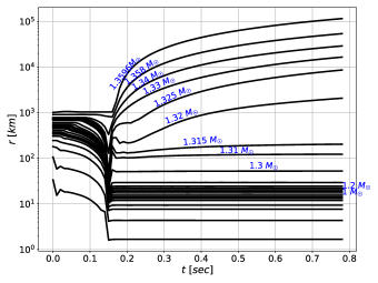
Figure 21: Trajectories of mass elements for the isentropic progenitor, with neutrino physics turned off. The collapse is induced by reducing the value of $Y_{e}$ to $0.2$ at the inner $5\times 10^{-2}\textup{M}_{\odot}$ of the progenitor, as it is otherwise stable in our simulations. Bounce and shock breakout occur only a few ms apart, indicative of the prompt mechanism. Only $\approx 0.05\textup{M}_{\odot}$ is ejected, a smaller amount compared to the case with neutrinos enabled, and comparable to the amount of ejecta in the work of Sharon & Kushnir (2020).

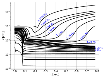
Figure 22: Trajectories of mass elements for the isentropic progenitor, with neutrino physics enabled. The initial value of $Y_{e}$ was reduced to $0.2$ at the inner $5\times 10^{-2}\textup{M}_{\odot}$ of the progenitor, as in Figure 21, for a fair comparison. Bounce occurs slightly earlier compared to the case without neutrinos, because electron capture expedites the collapse. There is a clear delay of nearly $150$ ms between the time of bounce and shock breakout, indicative of the delayed-neutrino mechanism. The amount of delay agrees with previous works. The amount of mass ejected is larger compared to the case without neutrinos.

References

- Arcavi et al. (2016) Arcavi, I., Wolf, W. M., Howell, D. A., et al. 2016, ApJ, 819, 35, doi: 10.3847/0004-637X/819/1/35
- Baron et al. (1987a) Baron, E., Cooperstein, J., & Kahana, S. 1987a, ApJ, 320, 300, doi: 10.1086/165541
- Baron et al. (1987b) Baron, E., Cooperstein, J., Kahana, S., & Nomoto, K. 1987b, ApJ, 320, 304, doi: 10.1086/165542
- Beniamini & Piran (2016) Beniamini, P., & Piran, T. 2016, MNRAS, 456, 4089, doi: 10.1093/mnras/stv2903
- Blinnikov (2017) Blinnikov, S. 2017, in Handbook of Supernovae, ed. A. W. Alsabti & P. Murdin, 843, doi: 10.1007/978-3-319-21846-5_31
- Burgay et al. (2003) Burgay, M., D’Amico, N., Possenti, A., et al. 2003, Nature, 426, 531, doi: 10.1038/nature02124
- Burrows & Lattimer (1986) Burrows, A., & Lattimer, J. M. 1986, ApJ, 307, 178, doi: 10.1086/164405
- Burrows et al. (2006) Burrows, A., Reddy, S., & Thompson, T. A. 2006, Nuclear Phys. A, 777, 356, doi: 10.1016/j.nuclphysa.2004.06.012
- Dall’Osso et al. (2014) Dall’Osso, S., Piran, T., & Shaviv, N. 2014, MNRAS, 438, 1005, doi: 10.1093/mnras/stt2188
- De et al. (2018) De, K., Kasliwal, M. M., Ofek, E. O., et al. 2018, Science, 362, 201, doi: 10.1126/science.aas8693
- Deller et al. (2009) Deller, A. T., Bailes, M., & Tingay, S. J. 2009, Science, 323, 1327, doi: 10.1126/science.1167969
- Drout et al. (2014) Drout, M. R., Chornock, R., Soderberg, A. M., et al. 2014, ApJ, 794, 23, doi: 10.1088/0004-637X/794/1/23
- Fox & Smith (2019) Fox, O. D., & Smith, N. 2019, Monthly Notices of the Royal Astronomical Society, 488, 3772, doi: 10.1093/mnras/stz1925
- Fryer et al. (1999) Fryer, C., Benz, W., Herant, M., & Colgate, S. A. 1999, ApJ, 516, 892, doi: 10.1086/307119
- Hillebrandt et al. (1984) Hillebrandt, W., Nomoto, K., & Wolff, R. G. 1984, A&A, 133, 175
- Jones et al. (2013) Jones, S., Hirschi, R., Nomoto, K., et al. 2013, ApJ, 772, 150, doi: 10.1088/0004-637X/772/2/150
- Kitaura et al. (2006) Kitaura, F. S., Janka, H. T., & Hillebrandt, W. 2006, A&A, 450, 345, doi: 10.1051/0004-6361:20054703
- Kramer et al. (2006) Kramer, M., Stairs, I. H., Manchester, R. N., et al. 2006, Science, 314, 97, doi: 10.1126/science.1132305
- Leung et al. (2021) Leung, S.-C., Fuller, J., & Nomoto, K. 2021, ApJ, 915, 80, doi: 10.3847/1538-4357/abfcbe
- Lippuner & Roberts (2017) Lippuner, J., & Roberts, L. F. 2017, ApJS, 233, 18, doi: 10.3847/1538-4365/aa94cb
- Livne (1993) Livne, E. 1993, ApJ, 412, 634, doi: 10.1086/172950
- Lyne et al. (2004) Lyne, A. G., Burgay, M., Kramer, M., et al. 2004, Science, 303, 1153, doi: 10.1126/science.1094645
- Lyutikov (2022) Lyutikov, M. 2022, MNRAS, doi: 10.1093/mnras/stac1717
- Lyutikov & Toonen (2019) Lyutikov, M., & Toonen, S. 2019, MNRAS, 487, 5618, doi: 10.1093/mnras/stz1640
- Mayle & Wilson (1988) Mayle, R., & Wilson, J. R. 1988, ApJ, 334, 909, doi: 10.1086/166886
- Moriya et al. (2013) Moriya, T. J., Blinnikov, S. I., Tominaga, N., et al. 2013, MNRAS, 428, 1020, doi: 10.1093/mnras/sts075
- Moriya et al. (2017) Moriya, T. J., Mazzali, P. A., Tominaga, N., et al. 2017, MNRAS, 466, 2085, doi: 10.1093/mnras/stw3225
- Müller et al. (2018) Müller, B., Gay, D. W., Heger, A., Tauris, T. M., & Sim, S. A. 2018, MNRAS, 479, 3675, doi: 10.1093/mnras/sty1683
- Nomoto (1984) Nomoto, K. 1984, ApJ, 277, 791, doi: 10.1086/161749
- Nomoto (1986) —. 1986, Annals of the New York Academy of Sciences, 470, 294, doi: 10.1111/j.1749-6632.1986.tb47981.x
- Nomoto (1987) —. 1987, ApJ, 322, 206, doi: 10.1086/165716
- O’Connor & Ott (2010) O’Connor, E., & Ott, C. D. 2010, Classical and Quantum Gravity, 27, 114103, doi: 10.1088/0264-9381/27/11/114103
- Özel & Freire (2016) Özel, F., & Freire, P. 2016, ARA&A, 54, 401, doi: 10.1146/annurev-astro-081915-023322
- Perley et al. (2019) Perley, D. A., Mazzali, P. A., Yan, L., et al. 2019, MNRAS, 484, 1031, doi: 10.1093/mnras/sty3420
- Piran & Shaviv (2005) Piran, T., & Shaviv, N. J. 2005, Phys. Rev. Lett., 94, 051102, doi: 10.1103/PhysRevLett.94.051102
- Podsiadlowski et al. (2004) Podsiadlowski, P., Langer, N., Poelarends, A. J. T., et al. 2004, ApJ, 612, 1044, doi: 10.1086/421713
- Pursiainen et al. (2018) Pursiainen, M., Childress, M., Smith, M., et al. 2018, MNRAS, 481, 894, doi: 10.1093/mnras/sty2309
- Rauscher & Thielemann (2000) Rauscher, T., & Thielemann, F.-K. 2000, Atomic Data and Nuclear Data Tables, 75, 1, doi: 10.1006/adnd.2000.0834
- Rauscher & Thielemann (2001) —. 2001, Atomic Data and Nuclear Data Tables, 79, 47, doi: 10.1006/adnd.2001.0863
- Sawada et al. (2021) Sawada, R., Kashiyama, K., & Suwa, Y. 2021, arXiv e-prints, arXiv:2112.10782. https://arxiv.org/abs/2112.10782
- Sharon & Kushnir (2020) Sharon, A., & Kushnir, D. 2020, ApJ, 894, 146, doi: 10.3847/1538-4357/ab8a31
- Shen et al. (1998a) Shen, H., Toki, H., Oyamatsu, K., & Sumiyoshi, K. 1998a, Nuclear Phys. A, 637, 435, doi: 10.1016/S0375-9474(98)00236-X
- Shen et al. (1998b) —. 1998b, Progress of Theoretical Physics, 100, 1013, doi: 10.1143/PTP.100.1013
- Suwa et al. (2015) Suwa, Y., Yoshida, T., Shibata, M., Umeda, H., & Takahashi, K. 2015, MNRAS, 454, 3073, doi: 10.1093/mnras/stv2195
- Tauris et al. (2013) Tauris, T. M., Langer, N., Moriya, T. J., et al. 2013, ApJ, 778, L23, doi: 10.1088/2041-8205/778/2/L23
- Tauris et al. (2015) Tauris, T. M., Langer, N., & Podsiadlowski, P. 2015, MNRAS, 451, 2123, doi: 10.1093/mnras/stv990
- Tauris et al. (2017) Tauris, T. M., Kramer, M., Freire, P. C. C., et al. 2017, ApJ, 846, 170, doi: 10.3847/1538-4357/aa7e89
- van den Heuvel (2007) van den Heuvel, E. P. J. 2007, in American Institute of Physics Conference Series, Vol. 924, The Multicolored Landscape of Compact Objects and Their Explosive Origins, ed. T. di Salvo, G. L. Israel, L. Piersant, L. Burderi, G. Matt, A. Tornambe, & M. T. Menna, 598–606, doi: 10.1063/1.2774916
- van den Heuvel (2011) van den Heuvel, E. P. J. 2011, Bulletin of the Astronomical Society of India, 39, 1
- Woosley & Baron (1992) Woosley, S. E., & Baron, E. 1992, ApJ, 391, 228, doi: 10.1086/171338