Symplectic circle actions on manifolds with contact type boundary

Abstract.

Many of the existing results for closed Hamiltonian $G$-manifolds are based on the analysis of the corresponding Hamiltonian functions using Morse-Bott techniques. In general such methods fail for non-compact manifolds or for manifolds with boundary.

In this article, we consider circle actions only on symplectic manifolds that have (convex) contact type boundary. In this situation we show that many of the key ideas of Morse-Bott theory still hold, allowing us to generalize several results from the closed setting.

Among these, we show that in our situation any symplectic group action is always Hamiltonian, we show several results about the topology of the symplectic manifold and in particular about the connectedness of its boundary. We also show that after attaching cylindrical ends, a level set of the Hamiltonian of a circle action is either empty or connected.

We concentrate mostly on circle actions, but we believe that with our methods many of the classical results can be generalized from closed symplectic manifolds to symplectic manifolds with contact type boundary.

Many of the classical results on Hamiltonian group actions are based on the study of the Hamiltonian functions with Morse-Bott methods: The fixed points of a Hamiltonian circle action are precisely the critical points of the corresponding Hamiltonian function, and its gradient flow partitions the symplectic manifold into even dimensional submanifolds. Among these results one finds for example [Ati82, GS82, McD88, AH91, Kar99] but also many others.

For non-compact manifolds or for manifolds that have non-empty boundary, Morse theory encounters serious problems. The reason for this is that gradient trajectories do not need to converge anymore to critical points, but may instead enter and leave the manifold at the boundary so that the topology of the underlying manifold cannot be controlled anymore by the critical points and their stable and unstable manifolds alone, and one needs to understand the behavior of the gradient vector field along the boundary.

Note that in contrast to Smale’s cobordism theory where the Morse function is an auxiliary tool that can be chosen to be constant on boundary components, the Morse-Bott function in our setup is given by the Hamiltonian group action, and cannot be modified without changing the action. For this reason, most results about Hamiltonian $\SS^{1}$-manifolds concerning closed symplectic manifolds, have only been generalized to Hamiltonian actions with proper moment maps.

In this article, we will deal with the case of compact Hamiltonian $\SS^{1}$-manifolds that have (convex) contact type boundary and Hamiltonian $\SS^{1}$-manifolds with cylindrical ends. This includes some physically relevant situations as for example the configuration space of many mechanical systems. As we will see the contact property implies that the boundary is also convex with respect to the gradient flow of the Hamiltonian function, that is, gradient trajectory cannot touch the boundary from the inside of the manifold. This fact alone gives us sufficient control on the gradient flow to work out Morse theoretic methods in case that all fixed points are confined to the interior of the symplectic manifold.

If the circle action does have fixed points on the boundary of the symplectic manifold, then we show that our Morse-Bott methods continue to work provided the corresponding gradient field satisfies in the neighborhood of the fixed points lying on the boundary an additional property. Circle actions on contact type boundaries automatically satisfy this additional assumption.

We have organized our article in the following way:

In Section 2, we explain how Morse-Bott theory behaves on manifolds that have boundary, assuming that none of the gradient trajectories touches the boundary from the inside. Here we do not make any reference to Hamiltonian group actions in the hope that our arguments might be interesting to researchers from other fields than symplectic geometry. Unknown to us, convexity and concavity with respect to gradient flows of Morse functions had already been studied much earlier [Mor29], see also the beautiful monograph [Kat20]. The situation we are interested in imposes on us to consider Morse-Bott functions, leading to several non-trivial complications that our knowledge had not been studied so far because there might be critical points on the boundary (see Example 2.4).

In Section 3, we apply then the results obtained in the previous section to Hamiltonian actions. For symplectic manifolds with contact type boundary we show that every symplectic action of a compact Lie group $G$ is automatically Hamiltonian, that is, every symplectic $G$-manifold admits a moment map.

Theorem A.

Let $G$ be a compact Lie group that acts symplectically on a compact symplectic manifold with non-empty contact type boundary. Then it follows that the action is Hamiltonian.

For a Hamiltonian $\SS^{1}$-manifold $W$ with contact type boundary, we distinguish the subsets $\xi^{+}$ and $\xi^{-}$ of the boundary, where the orbits of the circle action are positively transverse or negatively transverse to the contact structure. In the context of $3$-dimensional contact manifolds, this decomposition goes back to [Lut79]. We show that the properties of $\xi^{+}$ and $\xi^{-}$ are strongly related via the gradient flow to the circle action on the interior of the symplectic manifold.

Recall that the Hamiltonian of an $\SS^{1}$-action on a closed symplectic manifold will always have a unique component of local maxima and a unique component of local minima. In the case with contact type boundary, we show that there is either a unique component of $\xi^{+}$ and none of the critical points of the Hamiltonian is a local maximum, or there is a unique component of critical points that are local maxima, and $\xi^{+}$ is empty. An analogous statement holds for the connected components of local minima and $\xi^{-}$.

Theorem B.

Let $(W,\omega)$ be a connected compact Hamiltonian $\SS^{1}$-manifold with convex contact type boundary, and let $H\colon W\to{\mathbb{R}}$ be an associated Hamiltonian function.

(a) Then it follows that the set of critical points $\operatorname{Crit}(H)$ is equal to the set of fixed points $\operatorname{Fix}(\SS^{1})$ of the circle action. These decompose into finitely many connected components

$$\operatorname{Fix}(\SS^{1})=\bigsqcup_{j}C_{j}\;,$$

that intersect $\partial W$ transversely. A component $C_{j}$ of $\operatorname{Fix}(\SS^{1})$ is a closed symplectic submanifold if and only if $C_{j}\cap\partial W=\emptyset$, otherwise $C_{j}$ is a compact symplectic manifold with convex contact type boundary $\partial C_{j}=C_{j}\cap\partial W$.

(b) The choice of an $\SS^{1}$-invariant Liouville vector field along the boundary defines an invariant contact structure $\xi$ on $\partial W$. Let $X$ be the infinitesimal generator of the circle action. Decompose then the boundary of $W$ into the three subsets

$$\xi^{+} =\bigl{\{}p\in\partial W\bigm{|}\text{ $X(p)$ is positively transverse to $\xi_{p}$}\bigr{\}}\;,$$

$$\xi^{-} =\bigl{\{}p\in\partial W\bigm{|}\text{ $X(p)$ is negatively transverse to $\xi_{p}$}\bigr{\}}\text{ and }$$

$$\xi^{0} =\bigl{\{}p\in\partial W\bigm{|}\;X(p)\in\xi_{p}\bigr{\}}\;.$$

If $H^{\prime}=\lambda(X)$ is the Hamiltonian function of $X$ associated to the Liouville form $\lambda:=\iota_{Y}\omega$, then $\xi^{+}=\{H^{\prime}>0\}$, $\xi^{-}=\{H^{\prime}<0\}$, $\xi^{0}=\{H^{\prime}=0\}$.

The closed subset $\xi^{0}$ is composed of all fixed points in $\operatorname{Fix}(\SS^{1})\cap\partial W$ and all non-trivial isotropic $\SS^{1}$-orbits in $\partial W$. The fixed points in $\partial W$ form a finite collection of closed contact submanifolds. The non-trivial isotropic orbits form a finite union of cooriented disjoint hypersurfaces in $\partial W$ that separate $\xi^{-}$ on one side from $\xi^{+}$ on the other side, so that $\xi^{0}$ is nowhere dense in $\partial W$.

The hypersurfaces of non-trivial isotropic orbits do not need to be compact as their closure may contain fixed points. If this is the case, we can also not expect that the closure of the hypersurface is a smooth submanifold.

(c) The function $H$ is Morse-Bott, and all the Morse-Bott indices of the different components of $\operatorname{Crit}(H)$ are even.

Let $C_{j}$ be a fixed point component that intersects $\partial W$. It follows that $\partial C_{j}=C_{j}\cap\partial W$ necessarily lies in $\xi^{0}$. It is surrounded in $\partial W$ by $\xi^{+}$, if and only if $C_{j}$ is a local minimum of $H$. Similarly, $\partial C_{j}$ is surrounded by $\xi^{-}$, if and only if $C_{j}$ is a local maximum of $H$.

One of the following mutually exclusive statements holds:

• The set of critical points $\operatorname{Crit}(H)$ has a unique component $C_{\max}$ whose points are local maxima (a unique component $C_{\min}$ whose points are local minima) and $H$ is everywhere else on $W\setminus C_{\max}$ strictly smaller than on $C_{\max}$ (everywhere else on $W\setminus C_{\min}$ strictly larger than on $C_{\min}$), so that these local maxima (local minima) are actually the global ones.

  The subset $\xi^{+}$ is empty ($\xi^{-}$ is empty). The inclusion $C_{\max}\hookrightarrow W$ ($C_{\min}\hookrightarrow W$) induces a surjective homomorphism $\pi_{1}(C_{\max})\to\pi_{1}(W)$ ($\pi_{1}(C_{\min})\to\pi_{1}(W)$).

• None of the points in $\operatorname{Crit}(H)$ are local maxima (local minima), and $H$ takes its global maximum on $\xi^{+}\subset\partial W$ (its global minimum on $\xi^{-}$).

  The subset $\xi^{+}$ ($\xi^{-}$) is open, non-empty and connected. The inclusion $\xi^{+}\hookrightarrow W$ (or $\xi^{-}\hookrightarrow W$) induces a surjective homomorphism $\pi_{1}(\xi^{+})\to\pi_{1}(W)$ (or $\pi_{1}(\xi^{-})\to\pi_{1}(W)$).

Our initial aim with this project was to find symplectic manifolds with disconnected contact boundary. We do not know of any example of dimension$\geq 6$, but we can show that in dimension $4$ there aren’t any.

Theorem C.

A $4$-dimensional compact Hamiltonian $\SS^{1}$-manifold cannot have disconnected contact type boundary.

A compact symplectic manifold with a torus action also has always connected contact type boundary.

Theorem D.

Let $G$ be a compact Lie group of rank at least $2$. If $(W,\omega)$ is a connected compact Hamiltonian $G$-manifold with convex contact type boundary, then it follows that $\partial W$ cannot be disconnected.

It is well-known that the level sets of a Hamiltonian function that generates a circle action on a closed manifold is are connected or empty. For manifolds with contact type boundary, this claim turns out to be wrong but in LABEL:sec:_hamiltonian_circle_manifold_withcylindrical_ends_has_connected_level_sets we show that the statement can be saved by attaching cylindrical ends to the manifold. This includes for example cotangent bundles.

We prove:

Theorem E.

Let $(W,\omega)$ be a connected compact Hamiltonian $\SS^{1}$-manifold that has convex contact type boundary, and let $H\colon W\to{\mathbb{R}}$ be the Hamiltonian function of the circle action. Complete $W$ by attaching cylindrical ends with respect to some invariant Liouville field and denote the resulting manifold by $(\widehat{W},\widehat{\omega})$ and the extended Hamiltonian by $\widehat{H}$.

Then it follows that the level sets of $\widehat{H}$ are either connected or empty.

As an easy corollary, we obtain the convexity for ${\mathbb{T}}^{2}$-actions, see LABEL:sec:_hamiltonian_circle_manifold_with_cylindrical_ends_hasconnected_level_sets.

Corollary (Convexity for ${\mathbb{T}}^{2}$-actions).

Let $(\widehat{W},\widehat{\omega})$ be a symplectic manifold with cylindrical ends equipped with a Hamiltonian ${\mathbb{T}}^{2}$-action, as explained in Definition 9. The corresponding moment map image $\widehat{\mu}(\widehat{W})$ is then a convex set.

1. Definitions and preliminary remarks

Let $G$ be a compact Lie group with Lie algebra ${\mathfrak{g}}$ that acts smoothly and effectively on a manifold $W$. To every $X\in{\mathfrak{g}}$, we associate the vector field

$$X_{W}(p):=\left.\tfrac{d}{dt}\right|_{t=0}\exp(tX)\cdot p$$

called the infinitesimal generator of $X$.

A (weakly) Hamiltonian action of $G$ on a symplectic manifold $(W,\omega)$ is a smooth action preserving the symplectic structure, and for which we can additionally associate to every $X\in{\mathfrak{g}}$ a function $H_{X}\colon W\to{\mathbb{R}}$ satisfying

$$\iota_{X_{W}}\omega=-dH_{X}\;.$$

The collection of Hamiltonian functions can be represented in a unified way by defining a moment map

$$\mu\colon W\to{\mathfrak{g}}^{*}$$

that satisfies $\langle\mu(p),X\rangle=H_{X}(p)$ for any $p\in W$, and any $X\in{\mathfrak{g}}$. Here $\langle\cdot,\cdot\rangle$ denotes the natural pairing between ${\mathfrak{g}}^{*}$ and ${\mathfrak{g}}$.

Every weakly Hamiltonian action admits a moment map: Simply choose a basis of ${\mathfrak{g}}$ given by elements $X_{1},\dotsc,X_{k}$, each with a Hamiltonian function $H_{1},\dotsc,H_{k}$, and define $\langle\mu(p),a_{1}X_{1}+\dotsm+a_{k}X_{k}\rangle=a_{1}\,H_{1}(p)+\dotsm+a_{k}\,H_{k}(p)$.

We say that a weakly Hamiltonian $G$-action is Hamiltonian, if it can be equipped with a moment map $\mu\colon W\to{\mathfrak{g}}^{*}$ that is $G$-equivariant. Here $G$ acts via the coadjoint representation on ${\mathfrak{g}}^{*}$, given for every $g\in G$, $X\in{\mathfrak{g}}$, and $\nu\in{\mathfrak{g}}^{*}$ by

(1.1) $$\langle\operatorname{Ad}_{g}^{*}\nu,X\rangle:=\langle\nu,\operatorname{Ad}_{g^{-1}}X\rangle\;.$$

For a circle action, a weakly Hamiltonian action is of course trivially Hamiltonian.

A symplectic manifold $(W,\omega)$ has (convex) contact type boundary $V=\partial W$ if there exists a Liouville vector field $Y$ in a neighborhood of $V$ that points transversely out of $W$. The vector field $Y$ induces a Liouville form $\lambda_{Y}:=\iota_{Y}\omega$ on the boundary collar which in turn determines a (cooriented) contact structure $\xi=\ker\bigl{(}{\left.{\lambda_{Y}}\right|_{TV}}\bigr{)}$ on $V$.

Note that $\alpha={\left.{\lambda_{Y}}\right|_{T\partial W}}$ is a contact form for $\xi$ that defines a volume form $\alpha\wedge(d\alpha)^{n-1}$ that is positive with respect to the boundary orientation of $\partial W$.

Example 1.1.

The most natural examples from classical mechanics are cotangent bundles with their natural actions induced by an action on the base manifold.

Let $L$ be any closed manifold carrying a Riemannian metric. The cotangent bundle $T^{*}L$ is a symplectic manifold with symplectic structure $d{\lambda_{\mathrm{can}}}$. This is the standard phase space of classical mechanics. A classical Hamiltonian function is of the form

$$H\colon T^{*}L\to{\mathbb{R}},\quad(x,\nu_{x})\mapsto\frac{{\mathopen{\lVert}\nu_{x}\mathclose{\rVert}}^{2}}{2m}+V(x)\;,$$

where $x\in L$ and $\nu_{x}\in T^{*}_{x}L$. The first term $\frac{1}{2m}\,{\mathopen{\lVert}\nu_{x}\mathclose{\rVert}}^{2}$ represents the kinetic energy of the system, and $V\colon L\to{\mathbb{R}}$ the potential energy.

We can define a Liouville vector field $Y$ by the equation $\iota_{Y}d{\lambda_{\mathrm{can}}}={\lambda_{\mathrm{can}}}$. Indeed, if $\pi\colon T^{*}L\to L$ is the natural bundle projection, the canonical Liouville form ${\lambda_{\mathrm{can}}}$ satisfies for every $(x,\nu_{x})\in T^{*}L$ and every $v\in T_{(x,\nu_{x})}T^{*}L$ the equation

$${\lambda_{\mathrm{can}}}(v)=\nu_{x}\bigl{(}d\pi_{(x,\nu_{x})}\,v\bigr{)}\;.$$

It is not hard to show that $Y$ is transverse to any level set of $H$ that does not intersect the $0$-section so that if we choose $C\gg 0$ large enough, the subdomain $H^{-1}\bigl{(}(-\infty,C]\bigr{)}$ yields a symplectic manifold with contact type boundary (the boundary being simply a constant energy level hypersurface).

Note that every diffeomorphism $\phi\colon L\to L$ lifts to a symplectomorphism $\Phi\colon T^{*}L\to T^{*}L$ given for every $x\in L$ and $\nu_{x}\in T_{x}^{*}L$ by

$$\Phi(x,\nu_{x}):=\bigl{(}\phi(x),\;\nu_{x}\circ(d\phi_{x})^{-1}\bigr{)}\in T_{\phi(x)}^{*}L\;,$$

where $d\phi_{x}\colon T_{x}L\to T_{\phi(x)}L$ is the differential of $\phi$ at the point $x$.

It follows that any smooth action of a Lie-group $G$ on $L$ induces a natural $G$-action on $T^{*}L$ by symplectomorphisms, and in fact, combining Lemma 3.2 with $\bigl{(}d\pi\,X_{T^{*}L}\bigr{)}(x,\nu_{x})=X_{L}(x)$, we obtain a $G$-equivariant moment map $\mu$ defined by

$$\langle\mu(x,\nu_{x}),X\rangle={\lambda_{\mathrm{can}}}\bigl{(}X_{T^{*}L}(x,\nu_{x})\bigr{)}=\nu_{x}\bigl{(}d\pi_{(x,\nu_{x})}X_{T^{*}L}(x,\nu_{x})\bigr{)}=\nu_{x}\bigl{(}X_{L}(x)\bigr{)}$$

for every $X$ in the Lie algebra of $G$, and every $(x,\nu_{x})\in T^{*}L$.

This shows that the $G$-action on $T^{*}L$ is always Hamiltonian. Additionally assuming that $G$ also preserves the energy function $H$, we obtain a Hamiltonian $G$-action on the symplectic domain $H^{-1}\bigl{(}(-\infty,C]\bigr{)}$ with contact type boundary.

2. Morse-Bott functions on manifolds with convex boundary

A classical result states that the Hamiltonian function of a circle action on a closed symplectic manifold is of Morse-Bott type, and the study of Hamiltonian actions on closed manifolds relies fundamentally on this fact. Unfortunately, Morse theory breaks down when considering non-compact manifolds or manifolds with boundary because gradient trajectories can escape, and cannot be controlled anymore.

In this article we are interested in symplectic manifolds that have contact type boundary. In this case we will show that the boundary is convex with respect to the gradient flow of the Hamiltonian function. Additionally we need a second fact that in our case will also always be satisfied: The stable set of a local maximum and the unstable set of a local minimum need to be submanifolds.

These two properties allow us to generalize many results from closed manifolds to our situation.

The description in this section is about gradient flows and does not make any reference to symplectic topology. We will discuss in how far the study of Morse-Bott functions on closed manifolds generalizes to compact manifolds whose boundary is convex with respect to the gradient field (see Definition 4). In the context of this article, we define a Morse-Bott function for a manifold with boundary as follows (for other possible definitions see [Lau11, Ori18]).

Definition 1.

Let $W$ be a compact manifold with boundary. We say that a smooth function $f\colon W\to{\mathbb{R}}$ is Morse-Bott if

• The set of its critical points $\operatorname{Crit}(f)$ is a disjoint union of finitely many smooth compact submanifolds

  $$\operatorname{Crit}(f)=\bigsqcup_{j}C_{j}$$

  that might possibly have boundary.

• If a component $C_{j}$ intersects $\partial W$ then it does so transversely and the boundary of $C_{j}$ is $\partial C_{j}=C_{j}\cap\partial W$. In particular, isolated critical points never lie in $\partial W$, and more generally the closed components of $\operatorname{Crit}(f)$ are those that do not intersect the boundary of $W$.

• The Hessian of $f$ is at every critical point $p\in C_{j}$ non-degenerate in the normal direction to $C_{j}$. At a boundary point $p\in\operatorname{Crit}(f)\cap\partial W$, we mean by this that the Hessian of ${\left.{f}\right|_{\partial W}}$ is non-degenerate when restricted to the normal direction of $\partial C_{j}$ in $\partial W$.

The index of $f$ at a component $C_{j}\subset\operatorname{Crit}(f)$ is the pair

$$\bigl{(}i^{-}(C_{j}),i^{+}(C_{j})\bigr{)}\;,$$

where $i^{-}(C_{j})$ is the number of negative eigenvalues of the Hessian, and $i^{+}(C_{j})$ is the number of positive eigenvalues of the Hessian, so that

$$\dim W=\dim C_{j}+i^{+}(C_{j})+i^{-}(C_{j})\;.$$

Remark 2.1.

Let $f$ be a Morse-Bott function on a compact manifold $W$ with boundary. Assume that $C_{j}$ is a component of $\operatorname{Crit}(f)$ that intersects $\partial W$ so that $\partial C_{j}=C_{j}\cap\partial W$ is a component of Morse-Bott type of the critical points $\operatorname{Crit}\bigl{(}{\left.{f}\right|_{\partial W}}\bigr{)}$ for the restricted function ${\left.{f}\right|_{\partial W}}$. The indices of $C_{j}$ in $W$ and the ones of $\partial C_{j}$ in $\partial W$ are related by

$$i^{-}(C_{j})=i^{-}(\partial C_{j})\;,\quad i^{+}(C_{j})=i^{+}(\partial C_{j})\;,\quad\text{ and }\quad\dim(C_{j})=\dim(\partial C_{j})+1\;.$$

Let $(W,g)$ be a compact Riemannian manifold that may have boundary, and let $f\colon W\to{\mathbb{R}}$ be any smooth function. Define the gradient vector field $\nabla f$ with respect to the metric $g$, and denote its flow by $\Phi^{\nabla f}_{t}$. Independently of whether $f$ is Morse-Bott, we can define the following stable and unstable subsets (that may or may not be submanifolds).

Let $A$ be any subset of $W$. We say that the gradient trajectory $\gamma(t)=\Phi^{\nabla f}_{t}(p)$ through $p\in W$ accumulates at $A$, if $\gamma$ exists for any positive time and if we find for every neighborhood $U$ of $A$, a time $T_{U}>0$ such that all $\gamma(t)$ with $t>T_{U}$ lie in $U$.

Definition 2.

The stable and unstable sets of a component $C_{j}\subset\operatorname{Crit}(f)$ are defined as

$$\begin{split}W^{s}(f;C_{j})&:=\bigl{\{}p\in W\bigm{|}\;\text{$\Phi_{\;t}^{\nabla f}(p)$ accumulates at $C_{j}$}\bigr{\}}\quad\text{ and }\\ W^{u}(f;C_{j})&:=\bigl{\{}p\in W\bigm{|}\;\text{$\Phi_{\;t}^{-\nabla f}(p)$ accumulates at $C_{j}$}\bigr{\}}\end{split}$$

respectively.

For Morse-Bott functions, a gradient trajectory converges on a closed manifold always to a critical point. This result which simplifies significantly the previous definition was explained to us by Krzysztof Kurdyka. The underlying idea going back to Łojasiewicz for analytic functions, see [Ło63] where applied to Morse-Bott functions in [KMP00].

Theorem 2.2 (Łojasiewicz).

Let $(W,g)$ be a compact Riemannian manifold that might possibly have boundary, and let $f\colon W\to{\mathbb{R}}$ be a Morse-Bott function.

If $\gamma$ is a gradient trajectory such that $\gamma(t)$ is defined for all $t\geq 0$, then it follows that $\gamma(t)$ converges for $t\to\infty$ to a critical point of $f$.

Proof.

The proof of this statement can be found in LABEL:section:Lojasiewicz of the appendix. We follow the explanations kindly given to us by Krzysztof Kurdyka. ∎

Thus if $f$ is a Morse-Bott function, we can equivalently characterize the stable and unstable sets of a component $C_{j}\subset\operatorname{Crit}(f)$ by

$$W^{s}(f;C_{j}):=\bigl{\{}p\in W\bigm{|}\;\lim_{t\to\infty}\Phi_{\;t}^{\nabla f}(p)\in C_{j}\bigr{\}}\quad\text{ and }\quad W^{u}(f;C_{j}):=\bigl{\{}p\in W\bigm{|}\;\lim_{t\to-\infty}\Phi_{\;t}^{\nabla f}(p)\in C_{j}\bigr{\}}$$

respectively.

It is a well-known fact that on closed manifolds, stable and unstable subsets of Morse-Bott functions are smooth submanifolds. This follows from the Hadamard-Perron theorem in combination with the fact that functions increase along their gradient trajectories. This is true even without assuming any particular form of the Riemannian metric close to the critical points. We state this result in Theorem B.4 in the appendix as a reference to deal later on with manifolds with boundary.

If $W$ has boundary, the flow of $X$ is usually not defined for all times $t\in{\mathbb{R}}$, and we denote for every point $p\in W$ the maximal time up to which $\Phi_{t}^{\nabla f}(p)$ exists in forward direction by $T_{\max}(p)$ and the maximal time in backward direction by $T_{\min}(p)$, so that $T_{\max}(p)\in[0,\infty)\cup\{+\infty\}$ and $T_{\min}(p)\in(-\infty,0]\cup\{-\infty\}$.

Definition 3.

The stable and unstable sets of a boundary component $\partial_{k}W$ are the subsets

$$W^{s}(f;\partial_{k}W) :=\bigl{\{}p\in W\bigm{|}\;\text{$T_{\max}(p)<\infty$ and $\Phi_{T_{\max}(p)}^{\nabla f}(p)\in\partial_{k}W$}\bigr{\}}$$

and

$$W^{u}(f;\partial_{k}W) :=\bigl{\{}p\in W\bigm{|}\;\text{$T_{\min}(p)>-\infty$ and $\Phi_{T_{\min}(p)}^{\nabla f}(p)\in\partial_{k}W$}\bigr{\}}$$

respectively.

Note that if $\Phi^{\nabla f}_{t}(p)$ tends for $t\to\infty$ to a critical point $p_{\infty}$ that lies in the intersection of a component $C_{j}\subset\operatorname{Crit}(f)$ with the boundary $\partial W$, then $p$ will clearly lie in the stable set of $C_{j}$, but by our definition it does not lie in the stable set of the boundary component: for this the boundary component has to be reached by the gradient trajectory in finite time (and stop there); converging to the boundary for $t\to\infty$ is not sufficient. In particular, all points of $\partial C_{j}$ lie in $W^{s}(f;C_{j})$, but not in $W^{s}(f;\partial_{k}W)$.

Lemma 2.3.

Let $(W,g)$ be a compact Riemannian manifold with boundary, and let $f\colon W\to{\mathbb{R}}$ be a Morse-Bott function. Then it follows that $W$ is partitioned by the stable sets

(2.1) $$W=\qquad\bigsqcup_{\mathclap{C_{j}\subset\operatorname{Crit}(f)}}W^{s}(f;C_{j})\qquad\bigsqcup\qquad\bigsqcup_{\mathclap{\partial_{k}W\subset\partial W}}W^{s}(f;\partial_{k}W)$$

where the $C_{j}$ and $\partial_{k}W$ are the different components of $\operatorname{Crit}(f)$ and $\partial W$ respectively. Analogously, $W$ is also partitioned by the corresponding unstable sets.

The proof of this lemma generalizes easily to any smooth function $f$ that does not need to be Morse-Bott but for which all components of $\operatorname{Crit}(f)$ are isolated in the interior of $W$.

Proof.

Let $p$ be any point in $W$, and let $\gamma$ be the gradient trajectory with $\gamma(0)=p$. If $\gamma$ is defined in forward direction only up to time $T_{\max}(p)<\infty$, then $\gamma$ necessarily hits one of the boundary components at $T_{\max}(p)$, and $p$ lies in the stable set of that component. If the flow is instead defined for all $t>0$, then it follows from Theorem 2.2 that $\gamma(t)$ converges for $t\to\infty$ to a critical point of $f$ so that $p\in W^{s}(f;C_{j})$ for some component $C_{j}$ of $\operatorname{Crit}(f)$.

This shows that every point in $W$ lies in the stable set of a boundary component $\partial_{k}W$ or in the stable set of a critical component $C_{j}$.

To prove that $W$ is partitioned by the stable sets, note firstly that a point cannot lie in the stable set of a boundary component and in the stable set of a critical point, because the first condition requires the flow only to exist for finite time while the other one requires that the flow exists for all times. Furthermore a point cannot lie in the stable sets of two different boundary components $\partial_{k}W$ and $\partial_{k^{\prime}}W$, because by our definition $p$ lies in $W^{u}(f;\partial_{k}W)$ if and only if the trajectory through $p$ ends on $\partial_{k}W$ (in finite time). The trajectory might intersect other boundary components before reaching the final one, but this is not sufficient to lie in their respective stable sets. Finally, $p$ lies in the stable set of a component $C_{j}$ of $\operatorname{Crit}(f)$ if the trajectory of $p$ converges to a point in $C_{j}$, thus excluding that it also converges to a point in another component of $\operatorname{Crit}(f)$.

The argument in backward time does not require any modifications and shows that the corresponding statement about the unstable sets is also true. ∎

We need to be more precise about the boundary: Let $W$ be a manifold with non-empty boundary, and let $X$ be a vector field on $W$. We distinguish the following three subsets that are determined by the behavior of $X$ along $\partial W$

$$\partial^{+}W :=\bigl{\{}p\in\partial W\bigm{|}\,\text{$X(p)$ points transversely out of $W$}\bigr{\}}\;,$$

$$\partial^{-}W :=\bigl{\{}p\in\partial W\bigm{|}\,\text{$X(p)$ points transversely into $W$}\bigr{\}}\;,$$

$$\partial^{0}W :=\bigl{\{}p\in\partial W\bigm{|}\,X(p)\in T_{p}(\partial W)\bigr{\}}\;.$$

Definition 4.

We say that the boundary of $W$ is convex with respect to the vector field $X$, if the maximal trajectory of $X$ of any point $p\in\partial^{0}W$ is just $p$ itself, that is, $X(p)$ either vanishes so that $\Phi_{t}^{X}(p)=p$ for all $t\in{\mathbb{R}}$ or if $X(p)\neq 0$, then the flow $\Phi_{t}^{X}(p)$ is not defined for any $t\neq 0$.

The intuition behind this definition is that if we embed $W$ into a slightly larger open manifold $\widehat{W}$, and then we extend the vector field $X$ smoothly to $\widehat{W}$, the convexity of $\partial W$ implies that the only non-trivial trajectories of $X$ that are tangent to $\partial W$ touch the boundary from the outside of $W$, see Figure 1.

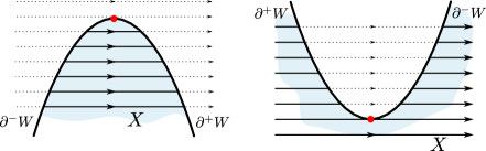
Figure 1. In the two cases depicted above, the domain $W$ is colored in blue, and the vector field $X$ has horizontal flow lines. On the left side, we have drawn the case of a boundary that is convex with respect to $X$. The vector field enters through $\partial^{-}W$ on one side and leaves again through $\partial^{+}W$ on the other side. It is only tangent to $\partial W$ at the red point, but touching $W$ from the outside its flow is neither defined (in $W$) for positive nor negative times. On the right side, $X$ also has a tangency with $\partial W$ in the red dot, but this time the flow comes from the interior of $W$, becomes tangent to $\partial W$, and then moves back into the interior of $W$ so that this boundary is not convex.

Example 2.4.

• Consider the vector field $X:=\partial_{x}$ on ${\mathbb{R}}^{2}$ so that the flow lines are horizontal lines. It is then easy to convince oneself that the closed unit disk (or any other geometrically convex domain) is convex with respect to $X$. For an annulus on the other hand, the inner boundary is not convex with respect to $X$.

• Consider again the closed annulus $A$ of all points $(x,y)$ in ${\mathbb{R}}^{2}$ with $1/2\leq x^{2}+y^{2}\leq 1$, and let $X=-x\,\partial x$ be the gradient vector field of the function $f(x,y)=-x^{2}/2$ with respect to the Euclidean metric.

  Note that against all intuition, this time $\partial A$ is convex, because $X$ vanishes at all boundary points where $X$ is not transverse to $\partial A$. This shows that convexity by itself is not sufficient to obtain for example results like the ones in Theorem 2.11. We will have to impose additionally properties on the vector field close to critical points lying on the boundary of the domain.

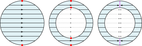
Figure 2. The left picture and the central picture show the two situations described in LABEL:example_convex_and_concaveboundary.(a). The disk is convex with respect to the horizontal flow, while the annulus isn’t. The picture on the right shows Example 2.4.(b). There is a vertical line of critical points, and the field points horizontally towards this line. Note that this example is also convex, because the gradient field is everywhere transverse to the boundary except for the points where the gradient vanishes.

In this article, we will be mostly interested in gradient vector fields. When there is no possible confusion we use the following notation.

Definition 5.

Let $(W,g)$ be a Riemannian manifold with boundary carrying a smooth function $f\colon W\to{\mathbb{R}}$. If $\partial W$ is convex with respect to $\nabla f$ we often say for simplicity that $\partial W$ is $\nabla$-convex.

The gradient vector field is almost everywhere transverse to a $\nabla$-convex boundary:

Lemma 2.5.

Let $(W,g)$ be a connected Riemannian manifold with boundary, and let $f\colon W\to{\mathbb{R}}$ be a non-constant Morse-Bott function such that $W$ has convex boundary with respect to $\nabla f$.

The subset of points where $\nabla f$ is transverse to the boundary is open and dense in $\partial W$. In particular, none of the boundary components of $W$ can lie in $\partial^{0}W=\bigl{\{}p\in\partial W\bigm{|}\,\nabla f(p)\in T_{p}(\partial W)\bigr{\}}$.

Proof.

Assume that $U\subset\partial W$ is an open set in $\partial W$ that lies in $\partial^{0}W$. If $p\in U$ were a point such that $\nabla f(p)\neq 0$, then attach a small collar to $W$ along $\partial W$ and extend $\nabla f$ smoothly to this enlarged manifold.

Choose a flow-box chart in ${\mathbb{R}}^{n}$ with coordinates $(x_{1},\dotsc,x_{n})$ such that $p$ corresponds to the origin and such that $\nabla f$ agrees with $\partial_{x_{1}}$. We can assume by a rotation of the coordinates that $\partial W$ is at the origin of the coordinate chart tangent to the hyperplane $\{x_{n}=0\}$. Then we can write $\partial W$ as a graph of a smooth function $h$, that is, $\partial W$ is parametrized by

$$(x_{1},\dotsc,x_{n-1})\mapsto\bigl{(}x_{1},\dotsc,x_{n-1},h(x_{1},\dotsc,x_{n-1})\bigr{)}$$

where $h$ is a function that vanishes at the origin, and whose differential also vanishes at the origin.

By our assumption that $\nabla f$ is everywhere along $U$ tangent to $\partial W$ it follows that $\partial_{x_{1}}h=0$ on a neighborhood of the origin so that $h$ does not depend on the $x_{1}$-coordinate. In particular, we obtain that $\gamma(s)=(s,0,\dotsc,0)$ is a segment of a non-trivial gradient trajectory that is contained in $\partial W$. This is a contradiction to the convexity assumption. We deduce that $\nabla f$ needs to vanish everywhere on $U$.

By our definition of Morse-Bott function, $\operatorname{Crit}(f)$ intersects $\partial W$ transversely. Thus if $U\subset\operatorname{Crit}(f)$, there would need to be a neighborhood of $p$ in $W$ that lied in $\operatorname{Crit}(f)$, and since $\operatorname{Crit}(f)$ is a finite union of submanifolds, it would follow that $W=\operatorname{Crit}(f)$ so that $f$ had to be constant. ∎

We can often verify the boundary convexity using the following (sufficient but not necessary) criterion.

Let $W$ be a manifold with boundary carrying a smooth vector field $X$. Choose a boundary collar of the form $(-\varepsilon,0]\times\partial W$ with coordinates $(s,p)$ such that $\{0\}\times\partial W$ corresponds to $\partial W$. The vector field $X$ is on this collar of the form

(2.2) $$X(s,p)=S(s,p)\,\partial_{s}+Z(s,p)\;,$$

where $S(s,p)$ is a smooth function, and $Z(s,p)$ is a vector field that is tangent to the slices $\{s_{0}\}\times\partial W$.

Clearly, it follows that $\partial^{\pm}W=\bigl{\{}p\in\partial W|\;\pm S(0,p)>0\bigr{\}}$, and $\partial^{0}W=\bigl{\{}p\in\partial W|\;S(0,p)=0\bigr{\}}$.

Definition 6.

The boundary $\partial W$ is strongly convex with respect to $X$, if $X$ given by LABEL:eq:_decomposition_of_vector_field_with_respectboundary_collar satisfies at every point $p\in\partial^{0}W$ either that

• $Z(0,p)$ vanishes or that

• $dS\bigl{(}Z\bigr{)}>0$.

Proposition 2.6.

Strong convexity implies convexity.

Proof.

Assume that $p\in\partial^{0}W$ so that $S(0,p)=0$. If $Z(0,p)=0$, then $X(p)=0$ and the trajectory through $p$ is constant and thus satisfies the definition of convexity.

If on the other hand $X(p)\neq 0$, then if follows in particular that $Z(0,p)\neq 0$. Extend $X$ smoothly to $(-\varepsilon,\varepsilon)\times\partial W$, and let $\gamma(t)=\bigl{(}s(t),p(t)\bigr{)}$ be the trajectory of $X$ through $\gamma(0)=(0,p)$. The convexity of $\partial W$ at $\gamma(0)$ is equivalent to the function $s(t)$ having a strict minimum at $t=0$.

Choose a chart for $\partial W$ that is centered at $p$ and that has coordinates ${\mathbf{x}}=(x_{1},\dotsc,x_{n})$ such that $Z(0,\dotsc,0)=\partial_{x_{1}}$. In these coordinates, the trajectory is of the form $\gamma(t)=\bigl{(}s(t);x_{1}(t),\dotsc,x_{n}(t)\bigr{)}$, where $s(t),x_{1}(t),\dotsc,x_{n}(t)$ are smooth functions satisfying $s(0)=x_{1}(0)=\dotsb=x_{n}(0)=0$, and

$$s^{\prime}(t)=S\bigl{(}s(t);x_{1}(t),\dotsc,x_{n}(t)\bigr{)}\;,\text{ and }x_{j}^{\prime}(t)=Z_{j}\bigl{(}s(t);x_{1}(t),\dotsc,x_{n}(t)\bigr{)}\text{ for all $j\in\{1,\dotsc,n\}$.}$$

A sufficient condition for $s(t)$ to have a strict minimum at $t=0$ is that $s^{\prime}(0)=0$ and $s^{\prime\prime}(0)>0$. The first condition is obviously satisfied, since $s^{\prime}(0)=S(0,\dotsc,0)=0$; for the second condition we compute

$$s^{\prime\prime}(0)=s^{\prime}(0)\cdot\frac{\partial S}{\partial s}(0,\dotsc,0)+\sum_{j=1}^{n}x_{j}^{\prime}(0)\cdot\frac{\partial S}{\partial x_{j}}(0,\dotsc,0)=\frac{\partial S}{\partial x_{1}}(0,\dotsc,0)\;.$$

Since $\frac{\partial S}{\partial x_{1}}(0,\dotsc,0)=dS(Z)>0$, the second condition is also verified. ∎

Definition 7.

Let $\partial^{+}W$, $\partial^{-}W$, and $\partial^{0}W$ be defined with respect to the gradient field $\nabla f$. Then we denote the stable subset of a connected component $\partial_{l}^{+}W$ of $\partial^{+}W$ by

$$W^{s}(f;\partial_{l}^{+}W) :=\bigl{\{}p\in W\bigm{|}\;\text{$T_{\max}(p)<\infty$ and $\Phi_{T_{\max}(p)}^{\nabla f}(p)\in\partial_{l}^{+}W$}\bigr{\}}\;,$$

and the unstable subset of a connected component $$\partial_{l}^{-}W \partial^{-}W$$ of by

$$W^{u}(f;\partial_{l}^{-}W) :=\bigl{\{}p\in W\bigm{|}\;\text{$T_{\min}(p)>-\infty$ and $\Phi_{T_{\min}(p)}^{\nabla f}(p)\in\partial_{l}^{-}W$}\bigr{\}}\;.$$

Unfortunately, if $C_{j}$ is a component of $\operatorname{Crit}(f)$ intersecting $\partial W$, then the stable and unstable subsets of $C_{j}$ will in general not be nicely embedded submanifolds (even assuming that $\partial W$ is $\nabla$-convex).

Consider again Example 2.4.(b). The gradient trajectories are horizontal segments pointing towards the $y$-axis. The stable set of the inner boundary is an open subset, but the stable set of the components of critical points are not. The reason is that the critical points that lie on the inner boundary have gradient trajectories that do not lie in the interior of the corresponding stable set. Note that no such problem appears at the critical points lying on the outer boundary.

This behavior is depicted in LABEL:fig:_stable_subset_is_manifold_ifboundary_suitable, and further illustrated by the elementary example below. The behavior does not only depend on the Morse-Bott function itself, but also on the choice of the Riemannian metric.

Example 2.7.

Let $f\colon W\to{\mathbb{R}}$ be a Morse-Bott function on a $2$-dimensional Riemannian manifold $(W,g)$ with boundary, and let $C$ be a $1$-dimensional component of $\operatorname{Crit}(f)$ intersecting $\partial W$.

Take a Morse-Bott chart with coordinates $(x,z)$ centered at a point $p\in C\cap\partial W$ such that $(x,0)$ corresponds to the boundary of $W$ and such that $f(x,z)=-x^{2}$ on this chart.

Assume the Riemannian metric $g_{1}$ to be of the form

$$g_{1}(x,z)=\begin{pmatrix}1&c\\ c&1\end{pmatrix}\;,$$

where $c$ is a constant such that $|c|<1$. The gradient vector field is then $\nabla_{1}f=\frac{2x}{1-c^{2}}\,(-1,c)$.

The sign of $2xc$ determines if $\nabla_{1}f$ points transversely into or out of $W$. The oriented trajectories of $\nabla_{1}f$ are for $x<0$ parallel to the vector $(1,-c)$, and for $x>0$ parallel to $(-1,c)$. Thus if $c>0$, then the stable set $W^{s}(f;C)$ of $C$ is the union of $\bigl{\{}x\leq 0,\;z\leq 0\bigr{\}}$ and $\bigl{\{}x>0,\;z\leq-cx\bigr{\}}$, that is, the stable set is not a neat submanifold of $W$. This situation corresponds to the behavior shown on the left side of LABEL:fig:_stable_subset_ismanifold_if_boundary_suitable.

Consider now instead the Riemannian metric $g_{2}$ of the form

$$g_{2}(x,z)=\begin{pmatrix}1&-cx\\ -cx&1\end{pmatrix}\;,$$

where $c$ is a constant such that $|c|<1$. The gradient vector field is then $\nabla_{2}f=-\frac{2x}{1-c^{2}x^{2}}\,(1,cx)$.

The oriented trajectories of $\nabla_{2}f$ are for $x<0$ parallel to the vector $(1,cx)$, and for $x>0$ parallel to $(-1,-cx)$. If $c>0$, then the stable set $W^{s}(f;C)$ fills up the entire chart, and in particular it is a neat submanifold of $W$. The considered situation is thus of the type shown on right side of LABEL:fig:stable_subset_is_manifold_if_boundary_suitable.

We will study now the properties of the different stable and unstable subsets. Under additional technical assumptions (that are always satisfied for Hamiltonian circle actions), we will be able to show that all stable/unstable subsets of maximal dimension, that is, the ones that correspond to local extrema or to the positive/negative boundary components are all mutually disjoint open subsets of $W$.

For some time, we had hoped that we could always choose a Riemannian metric that preserved the convexity of the boundary and such that all stable and unstable subsets of a Morse-Bott function would be smooth submanifolds. The Example 2.4.(b) contradicts Theorem 2.11 showing that our belief was wrong.

We call a point of $W$ that does not lie in $\partial W$, an interior point of $W$. Furthermore, if $A$ is a subset of $W$, we denote the set of all points in $A$ that are interior points of $W$, that is, $A\setminus\partial W$ by $\operatorname{Int}A$. In particular, $\operatorname{Int}W=W\setminus\partial W$.

Proposition 2.8.

Let $(W,g)$ be a compact Riemannian manifold with boundary, and let $f\colon W\to{\mathbb{R}}$ be a Morse-Bott function. Suppose that the boundary of $W$ is $\nabla$-convex, then the stable and unstable sets satisfy:

• All subsets $W^{s}(f;\partial_{l}^{+}W)$ and $W^{u}(f;\partial_{l}^{-}W)$ are open in $W$ and intersect $\partial W$ transversely.

• If $C_{j}\subset\operatorname{Crit}(f)$ is a component that may or may not intersect $\partial W$, then it follows that the interior of the stable and unstable sets $\operatorname{Int}W^{s}(f;C_{j})$ and $\operatorname{Int}W^{u}(f;C_{j})$ are contained in smooth submanifolds of dimension $\dim C_{j}+i^{-}(C_{j})$ and $\dim C_{j}+i^{+}(C_{j})$ respectively.

• If $C_{j}\subset\operatorname{Crit}(f)$ does not intersect $\partial W$, then it follows that

  $$W^{s}(f;C_{j})\quad\text{ and }\quad W^{u}(f;C_{j})$$

  are smooth submanifolds with boundary. Their respective dimensions are $\dim C_{j}+i^{-}(C_{j})$ and $\dim C_{j}+i^{+}(C_{j})$, and they intersect $\partial W$ transversely, and $\partial W^{s}(f;C_{j})\subset\partial W$ and $\partial W^{u}(f;C_{j})\subset\partial W$.

Proof.

The convexity assumption imposes that any non-trivial gradient trajectory intersecting the boundary of $W$ necessarily does so transversely. Thus if $p_{0}$ and $p_{1}$ are any two points in the interior of $W$ that lie on the same gradient trajectory $\gamma$, say with $\gamma(0)=p_{0}$ and $\gamma(T)=p_{1}$, then it follows that none of the points $\gamma(t)$ with $t\in[0,T]$ can intersect $\partial W$ so that $\gamma\bigl{(}[0,T]\bigr{)}$ lies in $\operatorname{Int}W$. It follows that there are open neighborhoods $U_{0}$ of $p_{0}$ and $U_{1}$ of $p_{1}$ such that $\Phi^{\nabla f}_{T}$ restricts to a diffeomorphism between $U_{0}$ and $U_{1}$.

(a) To show that $W^{s}(f;\partial_{l}^{+}W)$ is open, note first that transversality is an open property so that $\partial_{l}^{+}W$ is an open subset of $\partial W$. Let $p_{0}$ be a point that lies in $\partial_{l}^{+}W$, then we can choose a small open neighborhood $U$ of $p_{0}$ in $\partial W$, and an $\varepsilon>0$ such that $(t,p)\mapsto\Phi^{\nabla f}_{t}(p)$ defines a diffeomorphism of $(-\varepsilon,0]\times U$ onto a neighborhood of $p_{0}$ in $W$. We have thus found an open neighborhood of $p_{0}$ that lies in $W^{s}(f;\partial_{l}^{+}W)$.

If $p_{0}\in W^{s}(f;\partial_{l}^{+}W)$ is now an interior point of $W$, then let $\gamma$ be the gradient trajectory starting at $p_{0}$ intersecting $\partial_{l}^{+}W$ at time $t=T$. In order to avoid any technicalities due to the boundary, use that $\gamma(T)$ has a small open neighborhood $U$ that lies in $W^{s}(f;\partial_{l}^{+}W)$. If $T^{\prime}\in(0,T)$ is chosen sufficiently close to $T$, then $p_{1}=\gamma(T^{\prime})$ will lie in $U$. By our remark above, there are open neighborhoods $U_{0}$ of $p_{0}$ and $U_{1}$ of $p_{1}$ such that $\Phi^{\nabla f}_{T^{\prime}}$ is a diffeomorphism between $U_{0}$ and $U_{1}$. After possibly shrinking the size of $U_{1}$, we may assume that $U_{1}$ lies in $U$. Replace $U_{0}$ by $U_{0}:=\Phi^{\nabla f}_{-T^{\prime}}(U_{1})$, then by construction $U_{0}$ is a neighborhood of $p_{0}$ that lies in $W^{s}(f;\partial_{l}^{+}W)$ proving that $W^{s}(f;\partial_{l}^{+}W)$ is indeed an open subset.

(b) In order to avoid some of the technicalities arising along the boundary, cap-off $W$ using Lemma B.1 to obtain a closed manifold $W^{\mathrm{cap}}$ and a Morse-Bott function $f^{\mathrm{cap}}$ that extends $f$ to all of $W^{\mathrm{cap}}$. We can also extend $g$ to a metric $g^{\mathrm{cap}}$ on all of $W^{\mathrm{cap}}$. Denote the cap-off of $C_{j}$ in $\operatorname{Crit}(f^{\mathrm{cap}})$ by $C_{j}^{\mathrm{cap}}$. Then it follows that $W^{s}(f^{\mathrm{cap}};C_{j}^{\mathrm{cap}})$ is a smooth submanifold of dimension $\dim C_{j}+i^{-}(C_{j})$, see Theorem B.4. Since the intersection of any submanifold with an open set is still a submanifold, it follows that $\operatorname{Int}W^{s}(f;C_{j})$ is contained in the submanifold $W^{s}(f^{\mathrm{cap}};C_{j}^{\mathrm{cap}})\cap\operatorname{Int}W$.

(c) Let $C_{j}\subset\operatorname{Crit}(f)$ be a component of $\operatorname{Crit}(f)$ that does not intersect $\partial W$. Capping-off $(W,g)$ and $f$ to $(W^{\mathrm{cap}},g^{\mathrm{cap}})$ and $f^{\mathrm{cap}}$ as in (b), we obtain that $C_{j}^{\mathrm{cap}}=C_{j}$ and the stable subset $W^{s}(f^{\mathrm{cap}};C_{j})$ in $W^{\mathrm{cap}}$ is a smooth submanifold of dimension $\dim C_{j}+i^{-}(C_{j})$.

This reproves that $\operatorname{Int}W^{s}(f;C_{j})$ is contained in a smooth submanifold, but to show that $W^{s}(f;C_{j})$ itself is a smooth submanifold, we argue as follows: First we will show that $W^{s}(f^{\mathrm{cap}};C_{j})$ and $W^{s}(f;C_{j})$ agree on a sufficiently small neighborhood of $C_{j}$. For this choose small open neighborhoods $U_{0}$ and $U_{1}$ of $C_{j}$ as in LABEL:box_aroundcritical_component.(b) such that $U_{0}\subset U_{1}$ lie in $\operatorname{Int}W$ and such that every gradient trajectory of $\nabla f^{\mathrm{cap}}$ that passes through $U_{0}$ and later escapes from $U_{1}$ can never again return to $U_{0}$. It follows that every point $q\in U_{0}$ lying in $W^{s}(f^{\mathrm{cap}};C_{j})$, automatically also lies in $W^{s}(f;C_{j})$ showing that $W^{s}(f^{\mathrm{cap}};C_{j})\cap U_{0}\subset W^{s}(f;C_{j})$.

If $p$ is now any point in $W^{s}(f;C_{j})$, then we can choose $T>0$ such that $\gamma(T)=q\in W^{s}(f;C_{j})\cap U_{0}$. If $p\notin\partial W$, then $\gamma(t)$ does not touch for $t\in[0,T]$ the boundary of $W$ anywhere due to $\nabla$-convexity. By the remark at the beginning of this proof, there are open neighborhoods $U_{p}$ and $U_{q}$ of $p$ and $q$ respectively such that $\Phi_{T}^{\nabla f}$ is a diffeomorphism between $U_{p}$ and $U_{q}$. We can shrink $U_{q}$ so that it lies in $U_{0}$, and since $W^{s}(f^{\mathrm{cap}};C_{j})\cap U_{q}=W^{s}(f;C_{j})\cap U_{q}$, it follows that the later is a smooth submanifold.

We obtain from the invariance of $W^{s}(f;C_{j})$ under the gradient flow that $W^{s}(f;C_{j})\cap U_{p}=\Phi_{-T}^{\nabla f}\bigl{(}W^{s}(f;C_{j})\cap U_{q}\bigr{)}$ so that $\operatorname{Int}W^{s}(f;C_{j})$ is globally a smooth submanifold.

If $p\in W^{s}(f;C_{j})$ does lie in $\partial W$, then note that $\nabla f(p)$ necessarily points by $\nabla$-convexity transversely into $W$. This proves that $W^{s}(f^{\mathrm{cap}};C_{j})$ intersects $\partial W$ transversely at $p$, and $W^{s}(f^{\mathrm{cap}};C_{j})\cap\partial W$ is then in a neighborhood of $p$ a smooth hypersurface of $W^{s}(f^{\mathrm{cap}};C_{j})$ that is transverse to $\nabla f$. Let $\gamma$ be the gradient trajectory with $\gamma(0)=p$, and assume that $\gamma(T)=q\in W^{s}(f;C_{j})\cap U_{0}$. Note that by $\nabla$-convexity, $\gamma(t)$ does not intersect $\partial W$ for any $t\in(0,T]$. As above, we can choose neighborhoods $U_{p}$ of $p$ and $U_{q}$ of $q$ such that $W^{s}(f^{\mathrm{cap}};C_{j})\cap U_{p}=\Phi_{-T}^{\nabla f^{\mathrm{cap}}}\bigl{(}W^{s}(f;C_{j})\cap U_{q}\bigr{)}$.

The subset $W^{s}(f^{\mathrm{cap}};C_{j})\cap U_{p}$ is split by the hypersurface $W^{s}(f^{\mathrm{cap}};C_{j})\cap\partial W$ into the part that lies in $W$ and the part that lies in the complement of $W$. The gradient trajectories of the points in the first half cannot touch $\partial W$ by $\nabla$-convexity from the interior, and thus it follows that they all lie in $W^{s}(f;C_{j})$.

This shows that $W^{s}(f;C_{j})$ is a smooth submanifold with boundary such that $\partial W^{s}(f;C_{j})\subset\partial W$, and such that $W^{s}(f;C_{j})$ intersects $\partial W$ transversely.

To prove the statements about the unstable sets, it suffices to invert the sign of $f$. ∎

Above we have shown that the stable set of a component of $\operatorname{Crit}(f)$ intersecting $\partial W$ is always contained in a submanifold whose dimension is given by the usual index formula. In general though, it does not need to be a submanifold itself. The following lemma provides a technical condition that solves this problem.

Lemma 2.9.

Let $(W^{\prime},g^{\prime})$ be a closed Riemannian manifold, and let $f^{\prime}\colon W^{\prime}\to{\mathbb{R}}$ be a Morse-Bott function. Suppose that $W$ is a compact subdomain with $\nabla$-convex boundary.

Consider a component $C^{\prime}_{j}$ of $\operatorname{Crit}(f^{\prime})$ that intersects $\partial W$ transversely, and denote the restriction of $f^{\prime}$ to $W$ by $f$, and the intersection $C^{\prime}_{j}\cap W\subset\operatorname{Crit}(f)$ by $C_{j}$.

• If $C_{j}\cap\partial W$ admits a neighborhood $U^{-}$ in $\partial W$ such that $\nabla f$ does not point anywhere along $W^{s}\bigl{(}\hat{f};C^{\prime}_{j}\bigr{)}\cap U^{-}$ transversely out of $W$, see LABEL:fig:_stable_subset_is_manifold_if_boundarysuitable, then it follows that the interior $\operatorname{Int}W^{s}(f;C_{j})$ of the stable subset of $C_{j}$ in $W$ is a smooth submanifold of dimension $\dim C_{j}+i^{-}(C_{j})$.

• Similarly, if $C^{\prime}_{j}\cap\partial W$ admits a neighborhood $U^{+}$ in $\partial W$ such that $\nabla f$ does not point anywhere along $W^{u}\bigl{(}f^{\prime};C^{\prime}_{j}\bigr{)}\cap U^{+}$ transversely into $W$, then it follows that the interior $\operatorname{Int}W^{u}(f;C_{j})$ of the unstable subset of $C_{j}$ in $W$ is a smooth submanifold of dimension $\dim C_{j}+i^{+}(C_{j})$.

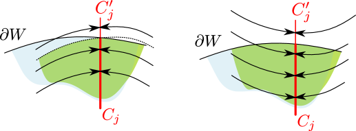
Figure 3. In the two pictures above, we have sketched in green color the stable set $\operatorname{Int}W^{s}(f;C_{j})$ of a component $C_{j}\subset\operatorname{Crit}(f)$ that intersects $\partial W$ transversely. According to LABEL:stable_sets_aresubmanifolds.(b), $\operatorname{Int}W^{s}(f;C_{j})$ is always contained in a submanifold, but in the left picture, we see that the stable set might be cut-off in an unfortunate way, while the picture on the right illustrates how the boundary condition stated in Lemma 2.9 avoids this problem.

Proof.

We will only consider stable sets; to prove the statements about the unstable ones, simply invert the sign of $f^{\prime}$. The stable set $W^{s}\bigl{(}f^{\prime};C^{\prime}_{j}\bigr{)}$ in $W^{\prime}$ is according to LABEL:stablesubset_smooth_on_closed_manifold a submanifold of dimension $\dim C^{\prime}_{j}+i^{-}(C^{\prime}_{j})$. We can choose arbitrarily small open neighborhoods $U_{0}\subset U_{1}$ of $C^{\prime}_{j}$ as in LABEL:box_aroundcritical_component.(b) such that

• a gradient trajectory of $\nabla f^{\prime}$ that passes through $U_{0}$ and later escapes from $U_{1}$ can never again return to $U_{0}$;

• the only critical points lying in $U_{1}$ are the ones in $C^{\prime}_{j}$.

We can furthermore suppose that $U_{1}$ is so small that

• the intersection of $U_{1}$ with $\partial W$ is contained in $U^{-}$.

We will first show that $\operatorname{Int}W^{s}(f;C_{j})\cap U_{0}=W^{s}(f^{\prime};C^{\prime}_{j})\cap U_{0}$ so that $\operatorname{Int}W^{s}(f;C_{j})\cap U_{0}$ is a smooth submanifold. The inclusion $W^{s}(f;C_{j})\subset W^{s}(f^{\prime};C^{\prime}_{j})$ is obvious, so assume that $p$ is any point in $\operatorname{Int}W^{s}(f^{\prime};C^{\prime}_{j})\cap U_{0}$. By our assumption, the $\nabla f^{\prime}$-trajectory through $p$ cannot escape from $U_{1}$, because otherwise it could never return to $U_{0}$ again, and $p$ would certainly not lie in the stable set of $C^{\prime}_{j}$. Since $U^{-}$ does not allow the trajectory to leave $U_{1}\cap\operatorname{Int}W$ either, we see that $p\in W^{s}(f;C_{j})$ as desired.

If $p$ is now any point in $\operatorname{Int}W^{s}(f;C_{j})$ and if $\gamma\subset W$ is its gradient trajectory, then it follows from Theorem 2.2 that $\gamma$ converges to a point on $C_{j}$. There is thus a time $T>0$ such that $\gamma(T)$ lies for every $t\geq T$ in the neighborhood $U_{0}$. Furthermore, by the convexity of the boundary, $\gamma$ does not intersect $\partial W$ on the interval $[0,T]$.

There is a small neighborhood $U_{p}$ of $p$ and a small neighborhood $U_{q}$ of $q=\gamma(T)$ such that $U_{q}\subset U_{0}\cap\operatorname{Int}W$ and such that $\Phi_{T}^{\nabla f}$ restricts to a diffeomorphism between $U_{p}$ and $U_{q}$. We have shown above that $\operatorname{Int}W^{s}(f;C_{j})\cap U_{0}=\operatorname{Int}W^{s}(f^{\prime};C^{\prime}_{j})\cap U_{0}$ so that also $W^{s}(f;C_{j})\cap U_{q}=W^{s}(f^{\prime};C^{\prime}_{j})\cap U_{q}$. We obtain that $W^{s}(f;C_{j})\cap U_{p}=\Phi_{-T}^{\nabla f}\bigl{(}W^{s}(f;C_{j})\cap U_{q}\bigr{)}$ is a smooth submanifold. ∎

The previous lemma is in general not very practical for direct applications, because to verify its conditions one would need to compute the intersection of the boundary with the stable subsets. The situation simplifies significantly, if the gradient field does not point anywhere in the neighborhood of $\partial C_{j}$ transversely out of $W$. For the main result of this section, LABEL:topology_simple_ifno_codim_1_stable_manifolds, it is even only necessary to show that the stable subsets of local maxima and the unstable subsets of local minima are open.

Corollary 2.10.

Let $(W,g)$ be a compact Riemannian manifold with boundary, and let $f\colon W\to{\mathbb{R}}$ be a Morse-Bott function such that $\partial W$ is $\nabla$-convex.

If $C_{j}$ is a component of $\operatorname{Crit}(f)$ that is a local maximum (a local minimum), and if either

• $\partial C_{j}=\emptyset$, or

• if $\partial C_{j}$ has a neighborhood $U_{j}$ in $\partial W$ such that $\nabla f$ does not point anywhere along $U_{j}$ transversely out of (into) $W$,

then it follows that $\operatorname{Int}W^{s}(f;C_{j})$ is an open subset of $\operatorname{Int}W$ ($\operatorname{Int}W^{u}(f;C_{j})$ is an open subset of $\operatorname{Int}W$).

Proof.

If $C_{j}$ does not intersect $\partial W$, then it follows from Proposition 2.8.(c) that $\operatorname{Int}W^{s}(f;C_{j})$ and $\operatorname{Int}W^{u}(f;C_{j})$ respectively are full dimensional submanifolds and thus open subsets. Otherwise if $C_{j}\cap\partial W\neq\emptyset$, take first the cap-off of $W$ and $f$ as in Lemma B.1, and then apply LABEL:lemma_forstable_sets_with_boundary so that we obtain again the desired claim. ∎

The assumptions about the intersection between local extrema and the boundary of the manifold made in Corollary 2.10 and in Theorem 2.11 below may seem quite artificial, but they are automatically satisfied by Hamiltonian circle actions so that the results developed in this section apply to the symplectic manifolds we are interested in.

Theorem 2.11.

Let $(W,g)$ be a connected compact Riemannian manifold with boundary, and let $f\colon W\to{\mathbb{R}}$ be a Morse-Bott function such that $\partial W$ is $\nabla$-convex.

We assume that none of the components $C_{j}\subset\operatorname{Crit}(f)$ has index $i^{-}(C_{j})=1$ ($i^{+}(C_{j})=1$). If $C_{j}$ is a local maximum (local minimum), then we additionally suppose that $C_{j}$ is either closed, or that its boundary $\partial C_{j}=C_{j}\cap\partial W$ has a neighborhood $U_{j}$ in $\partial W$ such that $\nabla f$ does not point anywhere along $U_{j}$ transversely out of $W$ (transversely into $W$).

Then we are in one of the following two situations:

• The set of critical points $\operatorname{Crit}(f)$ has a unique component $C_{\max}$ that is a local maximum (a unique component $C_{\min}$ that is a local minimum), and $f$ is everywhere else on $W\setminus C_{\max}$ strictly smaller than on $C_{\max}$ (everywhere else on $W\setminus C_{\min}$ strictly larger than on $C_{\min}$), so that this local maximum (local minimum) is actually the global one. The gradient field $\nabla f$ does not point anywhere along $\partial W$ transversely out of $W$ (into $W$). Finally, every loop in $W$ can be homotoped to one that lies in $C_{\max}$ (that lies in $C_{\min}$).

• The subset $\partial^{+}W$ ($\partial^{-}W$) is non-empty and connected, and every loop in $W$ can be homotoped to one that lies in $\partial^{+}W$ ($\partial^{-}W$). None of the components of $\operatorname{Crit}(f)$ is a local maximum (local minimum), and $f$ takes its global maximum (global minimum) on the boundary of $W$.

Proof.

Let $W_{0}$ be the union of all the stable sets of boundary components of $W$ and of all the stable sets of components $C_{j}\subset\operatorname{Crit}(f)$ that are local maxima. According to Lemma 2.3, the stable subsets partition $W$ so that the complement of $W_{0}$ is the union of all $\operatorname{Int}W^{s}(f;C_{k})$ for which $C_{k}\subset\operatorname{Crit}(f)$ is not a local maximum.

With our assumptions it follows from LABEL:stable_set_of_max_minopen that $\operatorname{Int}W^{s}(f;C_{j})$ is open for every component $C_{j}$ that is composed of local maxima. By the convexity assumption, the flow line of a point $p\in\operatorname{Int}W$ intersecting the boundary of $W$ will do so transversely so that $\operatorname{Int}W^{s}(f;\partial_{k}W)$ is the disjoint union of all $\operatorname{Int}W^{s}(f;\partial_{l}^{+}W)$ with $\partial_{l}^{+}W\subset\partial_{k}W$, and furthermore each of the stable subsets $\operatorname{Int}W^{s}(f;\partial_{l}^{+}W)$ is by Proposition 2.8.(a) open.

Thus we see that $\operatorname{Int}W_{0}$ decomposes into subsets that are open and pairwise disjoint. We will show that $\operatorname{Int}W_{0}$ is path-connected, so that all but one of the stable subsets composing $\operatorname{Int}W_{0}$ have to be empty.

Let $p$ and $p^{\prime}$ be any two points in the interior of $W_{0}$, and join them by a path $\gamma$ in $\operatorname{Int}W$. We can perturb $\gamma$ in such a way that it will lie in $\operatorname{Int}W_{0}$: if $C_{k}\subset\operatorname{Crit}(f)$ is a closed component, recall that by Proposition 2.8.(c) the interior of its stable subset $W^{s}(f;C_{k})$ is a smooth submanifold of dimension $\dim C_{k}+i^{-}(C_{k})$; if $C_{k}$ is a component of $\operatorname{Crit}(f)$ with $\partial C_{k}\neq\emptyset$, then its stable set $\operatorname{Int}W^{s}(f;C_{k})$ does not need to be a smooth submanifold, but by LABEL:stable_setsare_submanifolds.(b) it is nonetheless contained in a smooth submanifold of dimension $\dim C_{k}+i^{-}(C_{k})$. It follows that the complement of $\operatorname{Int}W_{0}$ in $\operatorname{Int}W$ lies in the finite union of smooth submanifolds that are each at least of codimension $2$.

A generic perturbation of $\gamma$ will be transverse to all of these submanifolds (see for example [Hir94, Theorem § 3.2.5]; it is not required that the submanifolds are closed). By the dimension formula, the intersection between $\gamma$ and any of the stable subsets $W^{s}(f;C_{k})$ in the complement of $W_{0}$ would be at most of dimension $-1$, that is, the intersection has to be empty. This shows that the perturbed path $\gamma$ is contained in $\operatorname{Int}W_{0}$ so that $\operatorname{Int}W_{0}$ is indeed path-connected.

We deduce that $\operatorname{Int}W_{0}$ is only composed of a single stable set, either $\operatorname{Int}W^{s}(f;\partial_{l}^{+}W)$ or $\operatorname{Int}W^{s}(f;C_{j})$ for $C_{j}$ a local maximum — all other potential stable sets composing $\operatorname{Int}W_{0}$ need to be empty. This proves that either there is a unique component of $\operatorname{Crit}(f)$ that is a local maximum or that $\partial^{+}W$ is non-empty and connected.

In order to prove that every loop $\gamma\subset W$ can be homotoped either to a loop in $\partial^{+}W$ or to a loop in $C_{\max}$, apply the same transversality argument as above to ensure that $\gamma$ lies in $\operatorname{Int}W_{0}$. Since $\operatorname{Int}W_{0}$ is composed of a single stable set, it retracts via the gradient flow either to $\partial^{+}W$ or to an arbitrarily small neighborhood of $C_{\max}$ thus proving the desired claim.

Finally note that since $W$ is compact $f$ takes somewhere a maximum, either in the interior of $W$ or on its boundary. If there is no component $C_{j}$ in $\operatorname{Crit}(f)$ that is a local maximum, then it is clear that the maximum of $f$ has to lie on $\partial W$.

If there is on the other hand a component $C_{\max}$, then $\partial^{+}W$ is empty by what we have just shown. The global maximum of $f$ cannot lie at a point of $\partial^{-}W$, because the gradient points along $\partial^{-}W$ transversely into $W$ so that the function is necessarily increasing in inward direction. Assume thus that the maximum lies at a point $p$ on $\partial^{0}W$. If $p$ is a regular point of $f$, then the level set of $p$ is locally a regular hypersurface that is transverse to $\partial W$. This implies that we find close to $p$ a point $p^{\prime}$ in $\operatorname{Int}W$ lying on the same level set as $p$ such that the level set is also regular in $p^{\prime}$. Following the gradient flow from $p^{\prime}$ the function $f$ increases further so that the global maximum cannot lie at $p^{\prime}$ and thus also not at $p$.

We deduce that if the global maximum lies on $\partial W$ it necessarily needs to lie at a point where $\nabla f$ vanishes, that is, it lies on a critical point of $f$. With our definition of Morse-Bott function, we know that every component of $\operatorname{Crit}(f)$ is transverse to $\partial W$ and thus it follows that $f$ takes its maximum on a component $C_{j}\subset\operatorname{Crit}(f)$. This component needs to be a local maximum so that $C_{j}=C_{\max}$ as desired.

The statements in parenthesis are easily deduced from the original ones by changing the sign of $f$. ∎

2.1. Closed $1$-forms of Morse-Bott type

Consider a connected Riemannian manifold $(W,g)$ with possibly non-empty boundary, and let $\eta$ be a closed $1$-form on $W$. We can define a vector field $X_{\eta}$ by the equation

$$g(X_{\eta},\cdot)=\eta\;.$$

Locally, every closed $1$-form is exact so that $X_{\eta}$ is locally a gradient vector field.

In this section we give a sufficient criterion for $\eta$ to be globally exact that we will then be used in Section 3.3 to prove that every compact symplectic $\SS^{1}$-manifold with contact type boundary is Hamiltonian (Theorem 3.18). The initial motivation for this theorem was a result due to McDuff [McD88] stating that a closed symplectic $\SS^{1}$-manifold is Hamiltonian if the $1$-form obtained as the contraction of the symplectic form with the infinitesimal generator of the circle action has a local maximum or minimum. We also reprove this result.

We will always assume in this section that $\eta$ is of Morse-Bott type, that is, the components of $\operatorname{Crit}(\eta)$ are smooth submanifolds, and the local primitives of $\eta$ around the critical points are of Morse-Bott type. If $W$ has non-empty boundary, then we assume additionally that the components of $\operatorname{Crit}(\eta)$ intersect $\partial W$ transversely.

The indices of a critical point of $\eta$ are simply the Morse-Bott indices of the corresponding local primitive and we say that a critical point of $\eta$ is a local maximum or local minimum if it is a local maximum or minimum of the local primitive.

The main result we want to prove in this section is the following theorem.

Theorem 2.12.

Let $\eta$ be a closed $1$-form of Morse-Bott type on a compact connected Riemannian manifold $(W,g)$. We assume that

• none of the critical points of $\eta$ has indices $i^{-}=1$ or $i^{+}=1$;

• $\partial W$ is either empty or convex with respect to $X_{\eta}$;

• every critical point $p$ that is a local maximum of $\eta$ and that lies in $\partial W$ admits an open neighborhood $U_{p}\subset\partial W$ in the boundary, such that $X_{\eta}$ does not point anywhere along $U_{p}$ out of $W$;

• every critical point $p$ that is a local minimum of $\eta$ and that lies in $\partial W$ admits an open neighborhood $U_{p}\subset\partial W$ in the boundary, such that $X_{\eta}$ does not point anywhere along $U_{p}$ into $W$.

If at least one of the two following conditions hold, then $\eta$ is exact:

• one of the components of $\operatorname{Crit}(\eta)$ is composed of local minima or local maxima;

• there exists a boundary component $\partial_{0}W$ of $W$ such that the restriction ${\left.{\eta}\right|_{\partial_{0}W}}$ is exact.

To prove this theorem, we will lift $\eta$ to the smallest covering space $\pi\colon\widetilde{W}\to W$ on which the lift of $\eta$ is exact. This way, we have a genuine Morse-Bott function on $\widetilde{W}$ that satisfies all properties required in Theorem 2.11 except of course for the compactness of $\widetilde{W}$. A uniqueness statement for local extrema or for boundary components of $\widetilde{W}$ as in Theorem 2.11 would force $\widetilde{W}\to W$ to be a simple cover as otherwise every local extremum or every boundary component in $W$ downstairs would lead to several such components upstairs. The main technical complication in our proof is thus to deal with the non-compactness of $\widetilde{W}$.

Construction of the cover $\widetilde{W}\to W$: Let $W$ be a smooth compact connected manifold with possibly non-empty boundary, and let $\eta$ be a closed $1$-form on $W$. Analogously to the construction of the universal cover, fix a point $x_{0}\in W$ and consider the set of all piecewise smooth paths $\Gamma=\bigl{\{}\gamma\colon[0,1]\to W\bigm{|}\;\gamma(0)=x_{0}\bigr{\}}$. We define an equivalence relation ”$\sim$” on $\Gamma$ by saying $\gamma\sim\gamma^{\prime}$ for $\gamma,\gamma^{\prime}\in\Gamma$, if and only if $\gamma(1)=\gamma^{\prime}(1)$ and $\int_{\gamma}\eta=\int_{\gamma^{\prime}}\eta$. Denote the space of equivalence classes by $\widetilde{W}:=\Gamma/\!\sim$, and note that there is a natural surjective map $\pi\colon\widetilde{W}\to W$ given by $\pi([\gamma])=\gamma(1)$.

To construct a smooth structure on $\widetilde{W}$, let $U_{x}$ be any open neighborhood of a point $x\in W$ such that ${\left.{\eta}\right|_{U_{x}}}$ is exact. We find for every $\tilde{x}\in\widetilde{W}$ with $\pi(\tilde{x})=x$, a natural lift $\rho_{\tilde{x}}\colon U_{x}\to\widetilde{W}$ such that $\rho_{\tilde{x}}(x)=\tilde{x}$ and $\pi\circ\rho_{\tilde{x}}=\operatorname{id}_{U_{x}}$. More precisely, if $\gamma\in\Gamma$ is a path representing $\tilde{x}$, then choose for any point $x^{\prime}\in U_{x}$, a path $\psi$ in $U_{x}$ connecting $x$ to $x^{\prime}$ and define $\rho_{\tilde{x}}(x^{\prime})$ as the point in $\widetilde{W}$ represented by the concatenation $\gamma\cdot\psi$. For any other choice of path $\psi^{\prime}\subset U_{x}$ connecting $x$ to $x^{\prime}$, we have $\int_{\psi^{\prime}}\eta=\int_{\psi}\eta$ so that $\gamma\cdot\psi\sim\gamma\cdot\psi^{\prime}$ which implies that $\rho_{\tilde{x}}$ does not depend on the choice of $\psi$. Similarly, one can also see that the construction does not depend on the choice of $\gamma$.

Furthermore if $\tilde{x}\neq\tilde{x}^{\prime}$ are any two points lying in the same fiber over $x$, then the images of $\rho_{\tilde{x}}$ and $\rho_{\tilde{x}^{\prime}}$ are disjoint, for otherwise, there would be a point $y\in U_{x}$ such that $\rho_{\tilde{x}}(y)=\rho_{\tilde{x}^{\prime}}(y)$. This way, if $\tilde{x}$ and $\tilde{x}^{\prime}$ are represented by paths $\gamma$ and $\gamma^{\prime}$ respectively, we obtain the points $\rho_{\tilde{x}}(y)$ and $\rho_{\tilde{x}^{\prime}}(y)$ by attaching to $\gamma$ and $\gamma^{\prime}$ respectively a path $\psi\subset U_{x}$ from $x$ to $y$. Since the integrals of $\eta$ over $\gamma\cdot\psi$ and $\gamma^{\prime}\cdot\psi$ agree by definition, the integrals over $\gamma$ and $\gamma^{\prime}$ also have to agree, implying that $\tilde{x}=\tilde{x}^{\prime}$.

With the help of these maps, we can lift any local structure from $W$ to $\widetilde{W}$. In particular, we can equip $\widetilde{W}$ with a topology such that $\pi\colon\widetilde{W}\to W$ is a covering space, and $\widetilde{W}$ carries a unique smooth structure coming from the base. We will always assume that $\widetilde{W}$ is equipped with the pull-back metric $\tilde{g}=\pi^{*}g$.

Furthermore, $\widetilde{W}$ is path-connected: Denote by $\tilde{x}_{0}\in\widetilde{W}$ the class of the constant path at $x_{0}$, and let $\tilde{x}$ be a point in $\widetilde{W}$ that is represented by a path $\gamma$. Consider the family of paths $\gamma_{s}$ for $s\in[0,1]$, given by

$$\gamma_{s}(t):=\begin{cases}\gamma(t),&t\in[0,s],\\ \gamma(s),&t\in[s,1].\end{cases}$$

For any fixed $s\in[0,1]$, $[\gamma_{s}]$ represents a point in $\widetilde{W}$, and the map $s\mapsto[\gamma_{s}]$ is a path in $\widetilde{W}$ that connects $\tilde{x}_{0}$ to $\tilde{x}=[\gamma]$.

Lemma 2.13.

Let $U\subset W$ be a connected open set on which $\eta$ is exact. Then, it follows that $\pi^{-1}(U)\to U$ is a trivial cover, that is, $\pi^{-1}(U)$ is for every choice of $x\in U$ naturally diffeomorphic to the disjoint union $\sqcup_{\tilde{x}\in\pi^{-1}(x)}\{\tilde{x}\}\times U$.

Proof.

As explained above, we find for every $\tilde{x}\in\widetilde{W}$ with $\pi(\tilde{x})=x$ a natural lift $\rho_{\tilde{x}}$. The images of two lifts $\rho_{\tilde{x}}$ and $\rho_{\tilde{x}^{\prime}}$ for two different points $\pi(\tilde{x})=\pi(\tilde{x}^{\prime})=x$ are disjoint.

This way we obtain $\pi^{-1}(U)=\sqcup_{\tilde{x}\in\pi^{-1}(x)}\rho_{\tilde{x}}(U)$. Since the $\rho_{\tilde{x}}$ were used to lift the smooth structure from $W$ to $\widetilde{W}$, we obtain by definition that each $\rho_{\tilde{x}}$ is a diffeomorphism showing the desired statement. ∎

Proposition 2.14.

The lift of $\eta$ to the covering $\widetilde{W}$ is exact. Furthermore, if $\tilde{f}\colon\widetilde{W}\to{\mathbb{R}}$ is a primitive of $\pi^{*}\eta$, it follows that two points $\tilde{x},\tilde{x}^{\prime}$ lying in the same fiber of $\pi$ are equal if and only if $\tilde{f}(\tilde{x})=\tilde{f}(\tilde{x}^{\prime})$.

Proof.

Define a function $\tilde{f}\colon\widetilde{W}\to{\mathbb{R}}$ by $\tilde{f}(\tilde{x}):=\int_{\gamma}\eta$, where $\gamma\in\Gamma$ is any path representing the point $\tilde{x}\in\widetilde{W}$. By our construction, $\tilde{f}$ is well-defined, and for every $x\in W$ and every contractible open neighborhood $U_{x}$ of $x$, we easily recognize that $\pi^{*}\eta=d\tilde{f}$ over $\pi^{-1}(U_{x})$. This proves that $\tilde{f}$ is a primitive of $\pi^{*}\eta$.

Let now $\tilde{x}$ and $\tilde{x}^{\prime}$ be two points in $\widetilde{W}$ lying in the same fiber over a point $x\in W$ such that $\tilde{f}(\tilde{x})=\tilde{f}(\tilde{x}^{\prime})$. If $\gamma\in\Gamma$ is a path representing $\tilde{x}$ and $\gamma^{\prime}\in\Gamma$ is a path representing $\tilde{x}^{\prime}$, then $x=\gamma(1)=\gamma^{\prime}(1)$. By our assumption $\tilde{f}(\tilde{x})=\int_{\gamma}\eta$ and $\tilde{f}(\tilde{x}^{\prime})=\int_{\gamma^{\prime}}\eta$ are equal. But this means precisely that $\gamma\sim\gamma^{\prime}$ represent the same point in $\widetilde{W}$, that is, $\tilde{x}=\tilde{x}^{\prime}$ as we wanted to show. ∎

Boundary convexity on $\widetilde{W}$: Let $(W,g)$ be a Riemannian manifold with possible non-empty compact boundary and let $\eta$ be a closed $1$-form on $W$ with dual vector field $X_{\eta}$ such that $g(X_{\eta},\cdot)=\eta$. Lift $\eta$ to the covering $(\widetilde{W},\tilde{g})$ constructed above. It follows by Proposition 2.14 that $\tilde{\eta}=\pi^{*}\eta$ admits a primitive function $\tilde{f}\colon\widetilde{W}\to{\mathbb{R}}$. The gradient vector field $\nabla\tilde{f}$ with respect to the pull-back metric $\tilde{g}$ is then related to $X_{\eta}$ by

(2.3) $$D\pi\cdot\nabla\tilde{f}=X_{\eta}\circ\pi\;.$$

For the corresponding flows we find

(2.4) $$\pi\circ\Phi_{t}^{\nabla\tilde{f}}=\Phi_{t}^{X_{\eta}}\circ\pi\;.$$

Lemma 2.15.

The boundary of $\widetilde{W}$ is $\partial\widetilde{W}=\pi^{-1}(\partial W)$, and the decomposition $\partial W=\partial^{+}W\cup\partial^{-}W\cup\partial^{0}W$ with respect to $X_{\eta}$ lifts to the decomposition $\partial\widetilde{W}=\partial^{+}\widetilde{W}\cup\partial^{-}\widetilde{W}\cup\partial^{0}\widetilde{W}$ with respect to $\nabla\tilde{f}$, that is,

$$\partial^{+}\widetilde{W}=\pi^{-1}(\partial^{+}W)\;,\quad\partial^{-}\widetilde{W}=\pi^{-1}(\partial^{-}W)\;,\text{ and }\partial^{0}\widetilde{W}=\pi^{-1}(\partial^{0}W)\;.$$

Moreover, $\partial W$ is (strongly) convex with respect to $X_{\eta}$, if and only if $\partial\widetilde{W}$ is (strongly) convex with respect to $\nabla\tilde{f}$.

Proof.

The claims in the lemma are all about local properties, and these are preserved because the covering is locally diffeomorphic to the base manifold. ∎

We are now ready to prove the main result of this section:

Proof of Theorem 2.12.

Let $\tilde{f}$ be a primitive of $\tilde{\eta}$ upstairs. To show that $\eta$ is exact, we will prove that the covering $\pi\colon\widetilde{W}\to W$ is simple so that $\pi$ is a diffeomorphism. Then $\tilde{f}\circ\pi^{-1}$ is a primitive of $\eta$ downstairs.

All local properties like being Morse-Bott etc. lift directly to $\widetilde{W}$. It thus follows that $\tilde{f}$ is a Morse-Bott function with $\operatorname{Crit}(\tilde{f})=\pi^{-1}\bigl{(}\operatorname{Crit}(\eta)\bigr{)}$, and none of the indices $i^{+}$ or $i^{-}$ of a point in $\operatorname{Crit}(\tilde{f})$ is equal to $1$. As explained in LABEL:convexityupstairs, the boundary $\partial\widetilde{W}$ is convex with respect to $\nabla\tilde{f}$, and every critical point $\tilde{p}\in\operatorname{Crit}(\tilde{f})\cap\partial\widetilde{W}$ that is a local maximum admits a neighborhood $U_{\tilde{p}}$ in $\partial\widetilde{W}$ such that $\nabla\tilde{f}$ does not point anywhere along $U_{\tilde{p}}$ transversely out of $\widetilde{W}$; every point $\tilde{p}\in\operatorname{Crit}(\tilde{f})\cap\partial\widetilde{W}$ that is a local minimum of $\tilde{f}$ admits a neighborhood $U_{\tilde{p}}$ in $\partial\widetilde{W}$ such that $\nabla\tilde{f}$ does not point anywhere along $U_{\tilde{p}}$ transversely into $\widetilde{W}$.

We will choose now values $a,b\in{\mathbb{R}}$ with $a<b$ to work with a suitable subdomain $\widetilde{W}_{[a,b]}=\tilde{f}^{-1}\bigl{(}[a,b]\bigr{)}$. The choice of these $a$ and $b$ depend on whether we are in case (a) or (b) below.

(a) Let $C\subset\operatorname{Crit}(\eta)$ be a component of critical points of $\eta$ consisting of local maxima. Clearly ${\left.{\eta}\right|_{C}}$ is exact, because $\eta$ vanishes along $C$. The restriction of $\eta$ to a tubular neighborhood $U$ retracting to $C$ is then also exact. If we assume that the covering map $\pi$ is not injective, then there are by LABEL:lemma_lift_of_exactneighborhood at least two components $\widetilde{C}_{1}$ and $\widetilde{C}_{2}$ of $\operatorname{Crit}(\tilde{f})$ that project diffeomorphically onto $C$. Furthermore, $\tilde{f}$ is constant on each of these components, but $\tilde{f}\bigl{(}\widetilde{C}_{1}\bigr{)}\neq\tilde{f}\bigl{(}\widetilde{C}_{2}\bigr{)}$.

Since $\widetilde{W}$ is path connected, there is a path $\tilde{\gamma}$ joining $\widetilde{C}_{1}$ to $\widetilde{C}_{2}$. We can choose the interval $[a,b]$ so large that the compact subset $\widetilde{C}_{1}\cup\widetilde{C}_{2}\cup\tilde{\gamma}$ is contained in $\tilde{f}^{-1}\bigl{(}[a,b]\bigr{)}$, and by Sard’s theorem, we can furthermore perturb $a$ and $b$ to be regular values both of the function $\tilde{f}$ and of ${\left.{\tilde{f}}\right|_{\partial\widetilde{W}}}$ so that $\tilde{f}^{-1}([a,b])$ is a smooth manifold with boundary and corners. To simplify the notation we restrict to the connected component of $\tilde{f}^{-1}([a,b])$ that contains $\widetilde{C}_{1}$ and $\widetilde{C}_{2}$ and denote it by $\widetilde{W}_{[a,b]}$.

If there is a component of $\operatorname{Crit}(f)$ that is a local minimum, we could equally well apply all arguments in this proof by replacing $\eta$ first by $-\eta$.

(b) Let $\partial_{0}W\subset\partial W$ be one of the connected components of the boundary on which $\eta$ is exact. Assume that the covering map $\pi$ is not injective. Applying LABEL:lemma_liftof_exact_neighborhood to a collar neighborhood of $\partial_{0}W$, we can find at least two boundary components $\partial_{1}\widetilde{W}$ and $\partial_{2}\widetilde{W}$ of $\partial\widetilde{W}$ that project diffeomorphically onto $\partial_{0}W$. In particular, it follows that $\partial_{1}\widetilde{W}$ and $\partial_{2}\widetilde{W}$ are compact.

Furthermore, if follows from LABEL:convex_boundary_cannot_beeverywhere_tangent_to_gradient (the argument is local) that $\nabla\tilde{f}$ cannot be everywhere tangent to $\partial_{1}\widetilde{W}$ or to $\partial_{2}\widetilde{W}$, and up to reversing the sign of $\eta$ if necessary, we may always assume that both boundary components have a point along which the gradient points outwards.

Since $\widetilde{W}$ is connected, there is a path $\tilde{\gamma}$ joining $\partial_{1}\widetilde{W}$ to $\partial_{2}\widetilde{W}$. Using that this path, that $\partial_{1}\widetilde{W}$, and that $\partial_{2}\widetilde{W}$ are compact and that $\tilde{f}$ is continuous, it follows that $\tilde{f}$ is bounded on $\partial_{1}\widetilde{W}\cup\partial_{2}\widetilde{W}\cup\tilde{\gamma}$, and in particular, we can find two real numbers $a$ and $b$ with $a<b$ such that $\partial_{1}\widetilde{W}\cup\partial_{2}\widetilde{W}\cup\tilde{\gamma}\subset\tilde{f}^{-1}([a,b])$. By slightly perturbing $a$ and $b$, we can again guarantee that $\tilde{f}^{-1}\bigl{(}[a,b]\bigr{)}$ will be a smooth manifold with boundary and corners, and we denote the component of $\tilde{f}^{-1}\bigl{(}[a,b]\bigr{)}$ containing $\partial_{1}\widetilde{W}$ and $\partial_{2}\widetilde{W}$ by $\widetilde{W}_{[a,b]}$.

Note that in both cases, $\widetilde{W}_{[a,b]}$ does not need to be compact. However, even so, we show in LABEL:no_gradienttrajectory_escapes_to_infinity below that the situation in the cover is sufficiently tame so that none of the gradient trajectories of $\tilde{f}$ can escape to infinity. This will be the key property that allows us to apply a strategy similar to the one used in the proof of Theorem 2.11 even though $\widetilde{W}_{[a,b]}$ may not be compact.

Denote $f^{-1}(a)\cap\widetilde{W}_{[a,b]}$ by $\widetilde{W}_{a}$ and $f^{-1}(b)\cap\widetilde{W}_{[a,b]}$ by $\widetilde{W}_{b}$. Study now a gradient trajectory $\tilde{\gamma}$ of $\widetilde{f}$ passing through an inner point of $\widetilde{W}_{[a,b]}$, and follow it for positive time inside $\widetilde{W}_{[a,b]}$ for as long as possible. By Proposition 2.16 below, the orbit $\tilde{\gamma}$ is contained in a compact subset of $\widetilde{W}_{[a,b]}$ so that precisely one of the following statements will be true for $\tilde{\gamma}$:

• $\tilde{\gamma}$ reaches in finite time $\widetilde{W}_{b}$, or some of the boundary components of $\partial\widetilde{W}\cap\widetilde{W}_{[a,b]}$;

• $\tilde{\gamma}(t)$ converges for $t\to\infty$ to a critical point of $\tilde{f}$ in $\widetilde{W}_{[a,b]}$ other than a local maximum;

• $\tilde{\gamma}(t)$ converges for $t\to\infty$ to a local maximum of $\tilde{f}$ lying in $\widetilde{W}_{[a,b]}$.

We will partition the interior of $\widetilde{W}_{[a,b]}$ according the cases listed above, and study the properties of this decomposition.

For case (A) note that the boundary of the domain $\widetilde{W}_{[a,b]}$ is composed of $\partial\widetilde{W}\cap\widetilde{W}_{[a,b]}$, of $\widetilde{W}_{a}$ and of $\widetilde{W}_{b}$. If $\tilde{\gamma}$ intersects $\partial\widetilde{W}_{[a,b]}$, it will necessarily do so transversely, because $\partial\widetilde{W}$ is $\nabla$-convex, and because $\widetilde{W}_{a}$ and $\widetilde{W}_{b}$ are regular level sets of $\tilde{f}$. Clearly, $\tilde{\gamma}$ cannot hit $\widetilde{W}_{a}$ or $\partial^{-}\widetilde{W}$ in forward time, because $\nabla\tilde{f}$ points along these boundary points into $\partial\widetilde{W}_{[a,b]}$. This also excludes that $\tilde{\gamma}$ reaches any of the corners in $\partial\widetilde{W}\cap\widetilde{W}_{a}$ or in $\partial^{-}\widetilde{W}\cap\widetilde{W}_{b}$. The remaining corners in $\partial\widetilde{W}\cap\widetilde{W}_{b}$ are composed of $\partial^{+}\widetilde{W}\cap\widetilde{W}_{b}$, and $\partial^{0}\widetilde{W}\cap\widetilde{W}_{b}$. Again by convexity, $\tilde{\gamma}$ cannot reach any point of $\partial^{0}\widetilde{W}$, and thus, $\tilde{\gamma}$ may only intersect corners given by $\partial^{+}\widetilde{W}\cap\widetilde{W}_{b}$ where $\nabla\tilde{f}$ is positively transverse both to $\partial\widetilde{W}$ and to $\widetilde{W}_{b}$.

Let $p\in\operatorname{Int}\widetilde{W}_{[a,b]}$ be a point whose gradient trajectory $\tilde{\gamma}$ satisfies (A). It follows that all trajectories through nearby points also end up on $\partial\widetilde{W}_{[a,b]}$: If $\tilde{\gamma}$ hits a point in $\partial\widetilde{W}$ or in $\widetilde{W}_{b}$ that is not a corner point, then the claim can be easily deduced from a consideration as in the proof of Proposition 2.8.(a); to see that the claim is true if $\tilde{\gamma}$ ends up at a corner point $q\in\partial^{+}\widetilde{W}\cap\widetilde{W}_{b}$ consider $\widetilde{W}_{[a,b+\varepsilon]}$, glue a collar to a neighborhood of $q$ in $\partial\widetilde{W}$, and extend $\widetilde{W}_{b}$ and the gradient vector field to this collar. Since $\nabla\tilde{f}$ hits both $\partial^{+}\widetilde{W}$ and $\widetilde{W}_{b}$ transversely, the gradient trajectory through any point close to $p$ will also hit both hypersurfaces transversely. Depending on whether it reaches first $\partial^{+}\widetilde{W}$ or first $\widetilde{W}_{b}$ or both at the same time, the trajectory will exit from $\widetilde{W}_{[a,b]}$ either through a point on $\partial^{+}\widetilde{W}$, through a point on $\widetilde{W}_{b}$ or through a corner point. In any case, any trajectory passing through a point close to $p$ will hit the boundary of $\widetilde{W}_{[a,b]}$ in positive time.

Thus the points in $\operatorname{Int}\widetilde{W}_{[a,b]}$ satisfying (A) form an open subset. Note that if not empty, $\partial_{1}\widetilde{W}$ and $\partial_{2}\widetilde{W}$ are disjoint and they are also isolated from the remaining points in $\partial\widetilde{W}_{[a,b]}$. In this case, we can further subpartition the points satisfying (A) into the open subsets of points whose trajectories end on $\partial_{1}\widetilde{W}$, the points whose trajectories end on $\partial_{2}\widetilde{W}$, and the ones ending on any of the remaining boundary points. Since we are assuming that $\nabla\tilde{f}$ is somewhere positively transverse both to $\partial_{1}\widetilde{W}$ and to $\partial_{2}\widetilde{W}$, it follows that the stable subsets corresponding to the first two components are not empty.

A point satisfying (B) lies on the stable subset of a component of $\operatorname{Crit}(\tilde{f})\cap\widetilde{W}_{[a,b]}$ that is not a local maximum. Our aim here is to show that each such stable subset is contained in a smooth submanifold of dimension at least $2$. If $\widetilde{W}$ were compact and without corners, this would directly follow from Proposition 2.8.(b). Nonetheless we will see below that such a statement also holds in our situation: Locally, we argue with the Hadamard-Perron Theorem [HPS77, Theorem 4.1]. If a component of $\operatorname{Crit}(\tilde{f})$ is closed then it admits a small neighborhood in which the local stable subset is a smooth submanifold with the desired properties. By LABEL:box_aroundcritical_component.(b), there exist two neighborhoods of $\widetilde{C}_{j}$ such that every point of $W^{s}(\tilde{f};\widetilde{C}_{j})$ in the smaller one of the two neighborhoods lies on the local stable subset given by the Hadamard-Perron Theorem. This shows that $W^{s}(\tilde{f};\widetilde{C}_{j})$ is close to $\widetilde{C}_{j}$ a smooth submanifold.

On a global level, there are also no problems with the stable subsets if $\widetilde{C}_{j}$ is closed, because the boundary of $\widetilde{W}_{[a,b]}$ is $\nabla$-convex in the sense that no gradient trajectory can touch the boundary from the interior. It follows that the gradient flow between two points lying in the interior of the manifold defines a diffeomorphism between their neighborhoods. The structure of the stable subset agrees thus at every point of $\operatorname{Int}\widetilde{W}_{[a,b]}$ with the manifold structure obtained locally around the critical points and thus $\operatorname{Int}W^{s}(\tilde{f};\widetilde{C}_{j})$ is a submanifold of codimension at least $2$.

If $\widetilde{C}_{j}$ is a component of $\operatorname{Crit}(\tilde{f})$ that does intersect $\partial\widetilde{W}$, then double first $\widetilde{W}_{[a,b]}$ along the boundary components intersecting $\widetilde{C}_{j}$ using the method presented in the proof of Lemma B.1. The potential problems due to the existence of corners are avoided by choosing a collar neighborhood that is tangent to $\widetilde{W}_{a}$ and $\widetilde{W}_{b}$. Note that $\operatorname{Crit}(\tilde{f})$ does never intersect the boundaries $\widetilde{W}_{a}$ and $\widetilde{W}_{b}$. After this extension of $\widetilde{W}_{[a,b]}$, $\widetilde{C}_{j}$ embeds into a closed component.

Furthermore note that because $\widetilde{C}_{j}$ is compact, we only need to double $\widetilde{W}_{[a,b]}$ along finitely many boundary components, and we can furthermore assume that any boundary component corresponding to $\partial\widetilde{W}$ or to its doubling is $\nabla$-convex, and that $\tilde{f}$ is regular along $\widetilde{W}_{a}$, $\widetilde{W}_{b}$, and along their doubles. We can apply the same steps as for closed components of $\operatorname{Crit}(\tilde{f})$, and it follows that the stable subset inside the doubled domain is a submanifold. When reducing back to $\widetilde{W}_{[a,b]}$, we retain then that $\operatorname{Int}W^{s}(\tilde{f};\widetilde{C}_{j})$ is contained is a submanifold of codimension at least $2$.

One easily convinces oneself that the points corresponding to situation (C) form an open subset. The argument that the stable set of every component of $\operatorname{Crit}(\tilde{f})$ that is a local maximum is contained in a full dimensional submanifold is identical to the proof given above for (B). By Corollary 2.10 it follows that such stable subsets are really submanifolds. Since none of the trajectories can touch the boundary from the inside, the presence of corners does not affect the validity of the claim.

Note that if there are two connected components $\widetilde{C}_{1}$ and $\widetilde{C}_{2}$ as described in case (a), then we can further subpartition all points satisfying (C) into the subsets $W^{s}(\tilde{f};\widetilde{C}_{1})$ and $W^{s}(\tilde{f};\widetilde{C}_{2})$ and the stable subsets of any remaining local maximum. Each of the parts in the decomposition is open.

Remove now all points that satisfy property (B) from $\operatorname{Int}\widetilde{W}_{[a,b]}$, and denote the complement by $\operatorname{Int}\widetilde{W}_{[a,b]}^{0}$. Since $\operatorname{Int}\widetilde{W}_{[a,b]}^{0}$ is the union of all points that verify properties (A) and (C), $\operatorname{Int}\widetilde{W}_{[a,b]}^{0}$ is open, and we will show now that it is also path connected: Choose any two points $p$ and $p^{\prime}$ in $\operatorname{Int}\widetilde{W}_{[a,b]}^{0}$ and connect them inside the larger set $\operatorname{Int}\widetilde{W}_{[a,b]}$ with a path $\gamma$. Note that $\operatorname{Crit}(\tilde{f})$ may decompose in $\operatorname{Int}\widetilde{W}_{[a,b]}$ into infinitely many components. Nonetheless $\gamma$ is compact and every gradient trajectory is contained by LABEL:no_gradienttrajectory_escapes_to_infinity in a ball of uniform radius. This implies that there is a compact set $K\subset\widetilde{W}_{[a,b]}$ such that $\gamma$ can only encounter the stable subsets of the components of $\operatorname{Crit}(\tilde{f})$ that intersect $K$. In particular it follows from this that $\gamma$ only intersects a finite number of different stable subsets.

Since every stable set $W^{s}(\tilde{f};\widetilde{C}_{k})$ corresponding to a component $\widetilde{C}_{k}$ that is not a local maximum, is contained in a submanifold of codimension at least $2$, we can assume after a perturbation that $\gamma$ does not intersect any of these stable sets. This implies in particular that $\gamma$ lies in $\operatorname{Int}\widetilde{W}_{[a,b]}^{0}$, proving as desired that $\operatorname{Int}\widetilde{W}_{[a,b]}^{0}$ is path connected.

Having shown that $\operatorname{Int}\widetilde{W}_{[a,b]}^{0}$ is a path connected set that is partitioned by the open subsets listed above for (A) and (C), it follows that only one of these open subsets may be non-empty. This leads to a contradiction both in situation (a) where $\partial_{1}\widetilde{W}$ and $\partial_{2}\widetilde{W}$ and in situation (b), where $\widetilde{C}_{1}$ and $\widetilde{C}_{2}$ are not empty. As desired we obtain that the cover $\widetilde{W}\to W$ has to be simple. ∎

Proposition 2.16.

Let $(W,g)$ be a compact manifold that might have boundary, and that carries a closed $1$-form $\eta$ of Morse-Bott type. Let $\pi\colon\widetilde{W}\to W$ be the minimal cover such that $\pi^{*}\eta$ is an exact $1$-form with primitive $\tilde{f}$, and let $a<b$ be regular values both of $\tilde{f}$ and of ${\left.{\tilde{f}}\right|_{\partial\widetilde{W}}}$.

Then there exists a constant $R>0$ such that every gradient trajectory of $\tilde{f}$ in $\widetilde{W}_{[a,b]}=\tilde{f}^{-1}([a,b])$ with respect to the pull-back metric $\tilde{g}:=\pi^{*}g$ lies in a ball of radius $R$. Furthermore, every gradient trajectory is of finite length.

Proof.

Before considering a gradient trajectory, let us first study the manifolds $W$ and $\widetilde{W}$ more in detail. Since the base manifold $W$ is compact, $\operatorname{Crit}(\eta)$ has only finitely many components $C_{1},\dotsc,C_{N}$.

Clearly $\eta$ vanishes along $C_{j}$, so that ${\left.{\eta}\right|_{C_{j}}}$ is trivially exact. We can find for every $C_{j}$ a tubular neighborhood and a function $f_{j}$ defined on this neighborhood such that $X_{\eta}$ is the gradient of $f_{j}$. By Lemma 2.13, it follows that the lift of $\pi^{-1}(C_{j})$ is a disjoint union of components of $\operatorname{Crit}(\tilde{f})$ and each of these components projects via $\pi$ diffeomorphically onto $C_{j}$. In particular, every component of $\operatorname{Crit}(\tilde{f})$ in $\widetilde{W}$ upstairs is compact.

More precisely, there exists for every component $C_{j}\subset\operatorname{Crit}(f)$ an $R_{j}>0$ such that any component $\widetilde{C}_{j}\subset\operatorname{Crit}(\tilde{f})$ covering $C_{j}$ is contained in a ball of radius smaller than $R_{j}$. To find a suitable radius for one such $\widetilde{C}_{j}$, it suffices to combine that $\widetilde{C}_{j}$ is compact with an exhaustion of $\widetilde{W}$ by open balls of increasing size.

To show that every component $\widetilde{C}_{j}^{\prime}$ of $\operatorname{Crit}(\tilde{f})$ covering $C_{j}$ also fits into a ball of radius $R_{j}$, let $\tilde{p}_{0}^{\prime}$ and $\tilde{p}_{1}^{\prime}$ be two points in $\widetilde{C}_{j}^{\prime}$. Project $\tilde{p}_{0}^{\prime}$ and $\tilde{p}_{1}^{\prime}$ down to $C_{j}\subset W$ and then lift them to points $\tilde{p}_{0}$ and $\tilde{p}_{1}$ in $\widetilde{C}_{j}$. There is then a path $\tilde{\psi}$ with $\tilde{\psi}(0)=\tilde{p}_{0}$ and $\tilde{\psi}(1)=\tilde{p}_{1}$ that is of length less than $R_{j}$. Project now this path to $W$, and lift it to a new path $\tilde{\psi}^{\prime}$ such that $\tilde{\psi}^{\prime}(0)=\tilde{p}_{0}^{\prime}$. The lifted path has the same length as the initial one, and it just remains to convince oneself that its end point $\tilde{\psi}^{\prime}(1)$ is $\tilde{p}_{1}^{\prime}$.

By Proposition 2.14, it suffices to verify that $\tilde{f}\bigl{(}\tilde{\psi}^{\prime}(1)\bigr{)}=\tilde{f}(\tilde{p}_{1}^{\prime})$. Since $\tilde{f}(\tilde{p}_{0}^{\prime})=\tilde{f}(\tilde{p}_{1}^{\prime})$, we can as well just check that $\tilde{f}\bigl{(}\tilde{\psi}^{\prime}(1)\bigr{)}-\tilde{f}\bigl{(}\tilde{\psi}^{\prime}(0)\bigr{)}=\int_{\tilde{\psi}^{\prime}}d\tilde{f}$ vanishes. This is true, because $\int_{\tilde{\psi}^{\prime}}d\tilde{f}=\int_{\pi\circ\tilde{\psi}^{\prime}}\eta=\int_{\tilde{\psi}}d\tilde{f}=\tilde{f}(\tilde{p}_{1})-\tilde{f}(\tilde{p}_{0})=0$.

Define $R_{0}=\max\{R_{1},\dotsc,R_{N}\}$.

Choose for every component $C_{j}$ neighborhoods $U_{j,0}\subset U_{j,1}$ as described in LABEL:function_increasesto_leave_box_around_critical_component that are sufficiently small so that the restriction of $\eta$ to $U_{j,1}$ is exact and such that no two $U_{i,1}$ and $U_{j,1}$ intersect for $i\neq j$. Using that the components of $\operatorname{Crit}(f)$ are compact, we can slightly enlarge $R_{0}$ (and shrink the size of $U_{j,1}$) so that every component of $\pi^{-1}\bigl{(}U_{j,1}\bigr{)}$ fits into a ball of size $R_{0}$.

We will now start working in $\widetilde{W}_{[a,b]}$. Denote by $\widetilde{U}_{0}$ the union in $\widetilde{W}_{[a,b]}$ of the small neighborhoods $\pi^{-1}(U_{j,0})\cap\widetilde{W}_{[a,b]}$ for $j=1,\dotsc,N$, and by $\widetilde{U}_{1}$ the union of all larger neighborhoods $\pi^{-1}(U_{j,1})\cap\widetilde{W}_{[a,b]}$ for $j=1,\dotsc,N$.

Let us now study a gradient trajectory $\tilde{\gamma}$ in $\widetilde{W}_{[a,b]}$ for positive time (for negative time, apply the same reasoning to $-\tilde{f}$). Let $I$ be the maximal interval on which $\tilde{\gamma}$ is defined, so that $I=[0,T_{\max})$ or $I=[0,T_{\max}]$. We will cover $I$ by two subsets $A$ and $B$ where

• $A$ is the union of all intervals in $\tilde{\gamma}^{-1}\bigl{(}\widetilde{U}_{1}\bigr{)}$ that contain at least one point that is mapped into the smaller neighborhood $\widetilde{U}_{0}$;

• $B$ is the union of all intervals in $\tilde{\gamma}^{-1}\bigl{(}\widetilde{W}_{[a,b]}\setminus\widetilde{U}_{0}\bigr{)}$ that each contain at least one point that is mapped into the complement of the larger neighborhood $\widetilde{U}_{1}$.

Clearly, if $\tilde{\gamma}(t)$ lies in $\widetilde{U}_{0}$ then it follows that $t$ lies in $A$; if $\tilde{\gamma}(t)$ lies in the complement of $\widetilde{U}_{1}$, then $t$ lies in $B$. The only remaining points are those for which $\tilde{\gamma}(t)$ lies in $\widetilde{U}_{1}\setminus\widetilde{U}_{0}$: if such a $t$ does neither lie in $A$ nor in $B$, it follows that we are in the particular case where $\tilde{\gamma}(I)$ lies entirely in one of the components of $\widetilde{U}_{1}\setminus\widetilde{U}_{0}$. Since each such component lies in a ball of radius $R_{0}$, it follows as desired that $\tilde{\gamma}$ is also contained in this ball.

If we exclude this particular situation, we find that $A$ and $B$ cover together all of $I$. Below we will show that the number of components of $A$ is bounded by some constant $N^{\prime}$ that is independent of the choice of $\tilde{\gamma}$. This obviously implies that the restriction of $\tilde{\gamma}$ to each component of $A$ is trapped in a ball of radius $R_{0}$.

The components of $A$ and $B$ alternate so that $B$ may have at most $N^{\prime}+1$ components. We will then show that the restriction of $\tilde{\gamma}$ to every component $B_{l}$ of $B$ has uniformly bounded length $\ell_{B}$ so that the total length of $\tilde{\gamma}(B)$ is bounded. Together these facts prove that $\tilde{\gamma}$ lies in a ball of uniformly bounded radius $R=R_{0}N^{\prime}+\ell_{B}\,(N^{\prime}+1)$.

We will now show that there is a uniform upper bound on the number of times a gradient trajectory of $\tilde{f}$ can move into the vicinity of $\operatorname{Crit}(\tilde{f})$ and then again again out of it. Let $f_{j}$ be the local primitive of $\eta$ on $U_{j,1}$ introduced above. By Lemma B.2.(b), it follows that an $X_{\eta}$-orbit that enters one of the components of $U_{j,0}$ either

• is trapped inside $U_{j,1}$, and hits $\partial W$ or it eventually accumulates at $C_{j}$,

• or it leaves $U_{j,1}$ and the value of $f_{j}$ increases on the way out of $U_{j,1}$ by more than some constant $\varepsilon_{j}>0$, see LABEL:function_increases_to_leave_box_around_criticalcomponent.

Since there are only finitely many components $C_{j}$, denote the minimum of the $\varepsilon_{1},\dotsc,\varepsilon_{N}$ by $\varepsilon_{0}$. The gradient trajectories of $\tilde{f}$ inherit these properties with respect to the components of the lifted neighborhoods $\widetilde{U}_{0}$ and $\widetilde{U}_{1}$ as can be easily deduced from Lemma 2.13.

This allows us to show that a gradient trajectory $\tilde{\gamma}$ cannot pass infinitely often from the smaller neighborhood $\widetilde{U}_{0}$ to the complement of the larger neighborhood $\widetilde{U}_{1}$. The reason is simply that every time $\tilde{\gamma}$ crosses one of the neighborhoods $\widetilde{U}_{0}$ and then escapes from the larger neighborhood $\widetilde{U}_{1}$, the function $\tilde{f}$ will increase by more than $\varepsilon_{0}>0$. Since the values of the function $\tilde{f}$ on $\widetilde{W}_{[a,b]}$ lie all in the interval $[a,b]$, none of the gradient trajectories in $\widetilde{W}_{[a,b]}$ can enter $\widetilde{U}_{0}$ and then leave $\widetilde{U}_{1}$ more than $N^{\prime}=\bigl{\lceil}(b-a)/\varepsilon_{0}\bigr{\rceil}+1$ times. In particular, $A$ cannot have more than $N^{\prime}$ components, and $B$ cannot have more than $N^{\prime}+1$ components.

Let us now study the restriction of $\tilde{\gamma}$ to a component $B_{0}$ of $B$, that is, $\tilde{\gamma}(B_{0})$ does not intersect the smaller neighborhood $\widetilde{U}_{0}$. Rescale $\nabla\tilde{f}$ on the complement of $\widetilde{U}_{0}$ to be of the form $Z=\frac{\nabla\tilde{f}}{\|\nabla\tilde{f}\|^{2}}$, and let $\widetilde{\psi}$ be the $Z$-trajectory that agrees up to parametrization with ${\left.{\tilde{\gamma}}\right|_{B_{0}}}$.

There is a $k>0$ bounding $\|X_{\eta}\|$ on the compact set $W\setminus\cup_{j}U_{j,0}$ from below. As a consequence, $\|Z\|<K$ with $K=1/k$ on the complement of $\widetilde{U}_{0}$. Furthermore we see from

$$\frac{d}{dt}\tilde{f}\bigl{(}\widetilde{\psi}(t)\bigr{)}=d\tilde{f}(Z)=1$$

that for every $t\in{\mathbb{R}}$ for which $\widetilde{\psi}(t)$ is defined

$$\tilde{f}\bigl{(}\widetilde{\psi}(t)\bigr{)}=\tilde{f}\bigl{(}\widetilde{\psi}(0)\bigr{)}+t\;.$$

Clearly, the trajectory $\widetilde{\psi}(t)$ can certainly not exist for times larger than $b-a$, because $\widetilde{\psi}(t)$ will either have hit $\widetilde{U}_{0}$, $\partial\widetilde{W}$ or $\widetilde{W}_{b}$ before. On the complement of $\widetilde{U}_{0}$, $\|Z\|$ is bounded by $K$ proving that $\widetilde{\psi}$ and thus also ${\left.{\tilde{\gamma}}\right|_{B_{0}}}$ are paths of finite length less than $K\,(b-a)$.

This completes the proof that $\tilde{\gamma}$ lies in a ball of radius $R=R_{0}N^{\prime}+K\,(b-a)\,(N^{\prime}+1)$.

It still remains to show that the length of $\tilde{\gamma}$ is bounded. Let $\gamma$ be the projection of $\tilde{\gamma}$ to $W$, and note that length of $\gamma$ and the one of $\tilde{\gamma}$ agree. Since $\|\gamma^{\prime}\|=\|X_{\eta}\|$ is bounded on the compact manifold $W$, it is clear that the only trajectories that could possibly have infinite length are those defined for all $t\in[0,\infty)$. Suppose thus from now on that $\tilde{\gamma}$ is of this type.

By what we proved above, $\tilde{\gamma}$ lies in a ball of radius $R$. By slightly varying the radius of the ball, and cutting off its complement, we can suppose that $\tilde{\gamma}$ lies in a compact domain with boundary and corners to which we can apply then the doubling trick in Lemma B.1 (the corners do not pose a problem as explained in the proof of LABEL:theorem:exactnesswith_boundary). Once in this situation, we obtain the desired result by Lemma A.2. ∎

2.2. Connectedness of level sets of a Morse-Bott function on a manifold with cylindrical ends

In the previous section we generalized several classical results about Morse-Bott functions on closed manifolds to Morse-Bott functions on compact manifolds with convex boundary.

By a classical result, every level set of a Hamiltonian function generating a circle action on a closed symplectic manifold is either connected or empty. This statement, which is one of the key steps for the proof of the Atiyah–Guillemin-Sternberg convexity theorem for Hamiltonian torus actions turns out to be false for manifolds with boundary, even assuming that the boundary is convex, see Example 3.24. To solve this minor technical problem, we attach cylindrical ends to our manifold. This will lead us in this section to Theorem 2.18.

The strategy to show that the level sets of the function $f$ are connected is to consider the flow of the vector field $Z=\frac{1}{{\mathopen{\lVert}\nabla f\mathclose{\rVert}}^{2}}\,\nabla f$. For closed manifolds, every point that lies in a level set $c_{0}$ is transported in time $t$ to the level set $c_{0}+t$ unless the point lies in one of the stable or unstable manifolds of critical points with value between $c_{0}$ and $c_{0}+t$. In our situation where the manifold has cylindrical ends and is hence not compact, the main technical difficulty will be to show that the trajectories of $Z$ can never escape in finite time to infinity.

Consider a non-compact manifold $\widehat{W}$ containing a compact domain $W$ with non-empty boundary $V=\partial W$ such that $\widehat{W}$ decomposes as

$$\widehat{W}=W\cup_{V}[0,\infty)\times V\;.$$

We call $[0,\infty)\times V$ the cylindrical ends of the manifold.

Definition 8.

Let $\hat{f}\colon\widehat{W}\to{\mathbb{R}}$ be a smooth function on a manifold

$$\widehat{W}=W\cup[0,\infty)\times V$$

with cylindrical ends. We say that $\hat{f}$ is adapted to the cylindrical end $[0,\infty)\times V$, if the restriction of $\hat{f}$ to the cylindrical end is of the product form

$${\left.{\hat{f}}\right|_{[0,\infty)\times V}}(s,p)=e^{s}\,f_{V}(p)+c\;,$$

where $c$ is locally constant (so that it is constant on each of the connected components of $V$), and $f_{V}\colon V\to{\mathbb{R}}$ is a smooth function on $V$.

We will from now on always assume in this section if not stated otherwise, that we have chosen a Riemannian metric $g$ on $\widehat{W}$ that restricts on $[0,\infty)\times V$ to

$${\left.{g}\right|_{[0,\infty)\times V}}=e^{s}\cdot\bigl{(}ds^{2}\oplus g_{V}\bigr{)}\;,$$

where $g_{V}$ is the restriction of $g$ to $V=\partial W$.

Remark 2.17.

A Riemannian metric of this form is geodesically complete.

Note that if $f_{V}$ is somewhere on $V$ strictly larger than $0$, then $\hat{f}$ is unbounded from above, if $f_{V}$ is somewhere on $V$ strictly smaller than $0$, then $\hat{f}$ is unbounded from below.

Let $\hat{f}$ be a function that is adapted to the cylindrical ends of $\widehat{W}$ so that it restricts on the ends to $e^{s}\,f_{V}(p)+c$, and let $g$ be a Riemannian metric such that ${\left.{g}\right|_{[0,\infty)\times V}}=e^{s}\cdot\bigl{(}ds^{2}\oplus g_{V}\bigr{)}$.

One easily verifies that the gradient of $\hat{f}$ simplifies on the cylindrical ends to

(2.5) $$\nabla\hat{f}(s,p)=f_{V}(p)\,\partial_{s}+\nabla f_{V}(p)\;,$$

where $\nabla f_{V}$ is the gradient vector field of $f_{V}$ on $V$ with respect to the metric $g_{V}$.

To determine a trajectory $\gamma(t)=\bigl{(}s(t),p(t)\bigr{)}$ of $\nabla\hat{f}$, integrate first the gradient flow of $f_{V}$ on $V$ to find $p(t)$. The $s(t)$-component is obtained in a second step by solving $s(t)=\int_{0}^{t}f_{V}(p(\tau))\,d\tau+s_{0}$.

We easily see from Equation 2.5 that a point $(s,p)\in[0,\infty)\times V$ in the cylindrical end is a critical point of $\hat{f}$ if and only if $p\in\operatorname{Crit}(f_{V})$ and $f_{V}(p)=0$. In particular, the critical set of $\hat{f}$ in the cylindrical ends is thus invariant under $s$-translations.

Note that $\hat{f}$ is a Morse-Bott function if and only if the restriction of $\hat{f}$ to the compact domain $W$ is a Morse-Bott function (so that $\operatorname{Crit}(\hat{f})$ is transverse to $\partial W$). In this case it follows that all critical points of $f_{V}$ lying in $f_{V}^{-1}(0)$ are also of Morse-Bott type (even though $f_{V}$ itself is usually not).

The main result we want to prove in this section is the following theorem.

Theorem 2.18.

Let $\widehat{W}$ be a manifold with cylindrical ends, and let $\hat{f}$ be a Morse-Bott function on $\widehat{W}$ that is adapted to the cylindrical ends and that does not have any critical points of index $i^{-}=1$ or $i^{+}=1$.

Then it follows that the level sets of $\hat{f}$ are either connected or empty.

We break up the proof into several steps. For this we assume from now on that $\widehat{W}$ is a manifold with cylindrical ends, that $\hat{f}$ is a smooth function on $\widehat{W}$ that is adapted to the cylindrical ends $[0,\infty)\times V$ so that it restricts to $\hat{f}(s,p)=e^{s}\,f_{V}(p)+c$ for $(s,p)\in[0,\infty)\times V$, and that $g$ is a Riemannian metric on $\widehat{W}$ that agrees on $[0,\infty)\times V$ with ${\left.{g}\right|_{[0,\infty)\times V}}=e^{s}\,\bigl{(}ds^{2}\oplus g_{V}\bigr{)}$.

Lemma 2.19.

• Let $(s_{0},p_{0})$ be a point in the cylindrical end at which $\nabla\hat{f}$ has strictly positive (strictly negative) $\partial_{s}$-component. Then it follows that the gradient trajectory $\gamma$ through this point has for all $t\geq 0$ strictly increasing $s$-coordinate (strictly decreasing $s$-coordinate for all $t\leq 0$), and in particular, $\gamma(t)$ stays for every $t\geq 0$ (for every $t\leq 0$) in the cylindrical end. Furthermore $\gamma(t)$ does not encounter any critical point, and tends to $s=+\infty$ as $t$ increases towards $t=+\infty$ (as $t$ decreases towards $t=-\infty$).

• The truncation of $\widehat{W}$ along any hypersurface $\{s_{0}\}\times\partial W$ in the cylindrical end is a compact domain $\widehat{W}_{\leq s_{0}}$ whose boundary is strongly convex with respect to $\nabla\hat{f}$.

Proof.

(a) The $\partial_{s}$-component of $\nabla\hat{f}$ at a point $(s,p)$ in the cylindrical end is $f_{V}(p)$, see LABEL:eq:gradient_in_cylindrical_end. If $(s_{0},p_{0})$ is a point at which $\nabla\hat{f}$ is positively transverse to the level set $\{s=s_{0}\}$, then $f_{V}(p_{0})>0$, and since ${\mathcal{L}_{\nabla\hat{f}}}f_{V}={\mathopen{\lVert}\nabla f_{V}\mathclose{\rVert}}^{2}\geq 0$, it follows that $f_{V}$ increases along the flow line from that moment on. In particular, the trajectory cannot hit any critical point in forward direction, since $f_{V}$ does not decrease.

Furthermore, the $s$-coordinate of the trajectory continues increasing so that it eventually hits $s=+\infty$ for $t\to+\infty$ (since $f_{V}$ is bounded, the trajectory cannot reach $s=+\infty$ in finite time). For the claim in parenthesis, just invert the sign of $\hat{f}$.

(b) Clearly $\nabla\hat{f}$ is only tangent to the boundary of the domain $\widehat{W}_{\leq s_{0}}$ along the subset $\partial^{0}\widehat{W}_{\leq s_{0}}=\{(s,p)|\;s=s_{0},\;f_{V}(p)=0\}$. According to Equation 2.5 and LABEL:def:strongly_convex, the boundary of $\widehat{W}_{\leq s_{0}}$ is strongly convex with respect to $\nabla\hat{f}$, because at every point $(s_{0},p)\in\partial^{0}\widehat{W}_{\leq s_{0}}$, either $\nabla f_{V}(p)=0$ so that $\nabla\hat{f}(s_{0},p)=0$, or $df_{V}(\nabla f_{V})={\mathopen{\lVert}\nabla f_{V}(s_{0},p)\mathclose{\rVert}}^{2}$ is strictly positive. ∎

As already explained, we will use a rescaled gradient flow in the proof of Theorem 2.18 to compare the different level sets of $\hat{f}$. The following lemma shows that the trajectories of this flow do not escape in finite time through the cylindrical end.

Lemma 2.20.

Consider the vector field

$$Z:=\frac{1}{{\mathopen{\lVert}\nabla\hat{f}\mathclose{\rVert}}^{2}}\cdot\nabla\hat{f}$$

defined on $\widehat{W}\setminus\operatorname{Crit}(\hat{f})$, let $x$ be any point in the domain of $Z$, and let $\gamma$ be the $Z$-trajectory through $x$. Then:

• If $x$ lies in the stable set $W^{s}(\hat{f};\widehat{C}_{j})$ of one of the connected components $\widehat{C}_{j}$ of $\operatorname{Crit}(\hat{f})$, then $\gamma$ is defined for time $[0,T_{x})$ with $T_{x}=\hat{f}\bigl{(}\widehat{C}_{j}\bigr{)}-\hat{f}(x)$, and $\gamma$ extends to a continuous map on $[0,T_{x}]$ such that $\gamma(T_{x})$ is a point in $\widehat{C}_{j}$.

• If $x$ does not lie in the stable set of any of the components of $\operatorname{Crit}(\hat{f})$, then $\gamma$ is defined for all $t>0$ and $\gamma(t)$ tends for $t\to\infty$ towards $s=+\infty$ in the cylindrical end of $\widehat{W}$.

Proof.

The vector fields $Z$ and $\nabla\hat{f}$ are conformal on $\widehat{W}\setminus\operatorname{Crit}(\hat{f})$ so that their trajectories agree up to reparametrization. This implies that any $Z$-trajectory that is confined in a compact domain of $\widehat{W}$, converges by Theorem 2.2 to some point in $\operatorname{Crit}(\hat{f})$ (this is the only time in this proof that we use that $\hat{f}$ is Morse-Bott).

Since ${\mathcal{L}_{Z}}\hat{f}=1$, a $Z$-trajectory moves any point in the level set $\{\hat{f}=c\}$ (whenever defined) in time $t$ to the level set $\{\hat{f}=c+t\}$. Thus it follows that if the trajectory through $x$ converges to a critical point $x^{\prime}$, the trajectory will only exist up to time $T_{x}:=\hat{f}(x^{\prime})-\hat{f}(x)$.

If the $Z$-orbit is not confined in a compact domain, it will necessarily move at a certain moment into the cylindrical end of $\widehat{W}$ crossing one of the $s$-level sets transversely in positive direction. We know from LABEL:cylindrical_end_convex_withrespect_to_gradient.(a) that the underlying gradient trajectory continues to move from this point on in the cylindrical end upwards towards $s=+\infty$. This implies that the $Z$-trajectory escapes through the cylindrical ends of $\widehat{W}$. Note though that to prove our claim, we also need to show that the trajectory needs infinite time to reach $s=+\infty$.

We will show below that the norm of $Z$ is bounded along any $Z$-trajectory that moves up towards $s=+\infty$. Since $\widehat{W}$ is by Remark 2.17 geodesically complete, the $Z$-trajectory cannot move in time $t>0$ further than distance $K\,t$, where ${\mathopen{\lVert}Z\mathclose{\rVert}}<K$. In particular, none of the $Z$-trajectories can escape through the cylindrical end of $\widehat{W}$ in finite time.

Recall from Equation 2.5 that $\nabla\hat{f}=f_{V}\,\partial_{s}+\nabla f_{V}$ on the cylindrical end. The norm of $Z$ on the cylindrical end is thus bounded by

$${\mathopen{\lVert}Z\mathclose{\rVert}}=\frac{1}{{\mathopen{\lVert}\nabla\hat{f}\mathclose{\rVert}}}=\frac{e^{-s/2}}{\sqrt{f_{V}^{2}+{\mathopen{\lVert}\nabla f_{V}\mathclose{\rVert}}_{V}^{2}}}\leq\frac{e^{-s/2}}{{\mathopen{\lvert}f_{V}\mathclose{\rvert}}}\;.$$

The function $f_{V}$ is monotonously increasing along the $Z$-trajectories because $df_{V}(Z)=\frac{{\mathopen{\lVert}\nabla f_{V}\mathclose{\rVert}}^{2}}{{\mathopen{\lVert}\nabla\hat{f}\mathclose{\rVert}}^{2}}\geq 0$. Thus, if $\gamma(t)=\bigl{(}s(t),p(t)\bigr{)}$ is a $Z$-trajectory in $[0,\infty)\times V$ such that $s^{\prime}(0)>0$, then ${\mathopen{\lVert}Z(\gamma(t))\mathclose{\rVert}}\leq K$ with $K=\frac{1}{{\mathopen{\lvert}f_{V}(p(0))\mathclose{\rvert}}}$ along this trajectory. ∎

In Proposition 2.8.(b) we showed for Morse-Bott functions on compact domains with $\nabla$-convex boundary that the interior of the stable and unstable subsets of the critical points are always contained in finite dimensional smooth submanifolds, but we did not claim that the stable and unstable subsets are actually smooth submanifolds themselves. For cylindrical Morse-Bott functions, we obtain the following stronger result.

Proposition 2.21.

Let $\widehat{C}_{j}$ be a connected component of $\operatorname{Crit}(\hat{f})$.

The stable and unstable sets are smooth submanifolds of dimension $\dim\widehat{C}_{j}+i^{-}(\widehat{C}_{j})$ and $\dim\widehat{C}_{j}+i^{+}(\widehat{C}_{j})$ respectively, where $i^{-}(\widehat{C}_{j})$ and $i^{+}(\widehat{C}_{j})$ are the indices of $\widehat{C}_{j}$. The level sets $\{s_{0}\}\times\partial W$ in the cylindrical end intersect the stable and unstable subsets transversely.

We have seen in Example 2.4.(b) that there exist compact domains with boundary for which the boundary is $\nabla$-convex with respect to some Morse-Bott function and some Riemannian metric, but for which the stable and unstable subsets are not smooth submanifolds. The situation complicates even even further because whether the stable or unstable subsets are smooth submanifolds depends also on the choice of the Riemannian metric, see LABEL:examplegradient_along_boundary_depends_on_metric. It might be difficult to decide if such a metric exists.

If we can find a boundary collar on which the Morse-Bott function resembles the product form of a cylindrical end, the situation simplifies:

Corollary 2.22.

Let $f\colon W\to{\mathbb{R}}$ be a Morse-Bott function on a compact manifold with boundary. Assume that $W$ has a boundary collar of the form $(-\varepsilon,0]\times\partial W$ on which $f$ restricts to $f(s,p)=e^{s}\,f_{V}(p)+C$, where $f_{V}$ is a function on $V:=\partial W$, and $C\in{\mathbb{R}}$ is a constant.

If we choose a Riemannian metric that agrees on the boundary collar with $e^{s}\,\bigl{(}ds^{2}\oplus g_{V}\bigr{)}$, then it follows that $W^{s}(f;C_{j})$ and $W^{u}(f;C_{j})$ are smooth proper submanifolds.

Proof of LABEL:stable_and_unstable_manifolds_in_cylindricalcompletion.

Truncate $\widehat{W}$ at any hypersurface $\{s_{0}\}\times\partial W$ to obtain a compact domain $\widehat{W}_{\leq s_{0}}$ whose boundary is convex with respect to $\nabla\hat{f}$, see LABEL:cylindrical_endconvex_with_respect_to_gradient.(b).

For a connected component $\widehat{C}_{j}$ of $\operatorname{Crit}(\hat{f})$ that does not intersect the boundary of $\widehat{W}_{\leq s_{0}}$, it follows from Proposition 2.8.(c) that the interior of the stable subset of $\widehat{C}_{j}$ in $\widehat{W}_{\leq s_{0}}$ is a smooth submanifold that we denote by $W^{\mathrm{stable}}_{<s_{0}}$. We show now that

$$W^{s}\bigl{(}\hat{f};\widehat{C}_{j}\bigr{)}\cap\widehat{W}_{<s_{0}}=W^{\mathrm{stable}}_{<s_{0}}\;.$$

Clearly $W^{\mathrm{stable}}_{<s_{0}}\subset W^{s}\bigl{(}\hat{f};\widehat{C}_{j}\bigr{)}$. On the other hand, let $p\in W^{s}\bigl{(}\hat{f};\widehat{C}_{j}\bigr{)}$ be a point that lies in $\widehat{W}_{<s_{0}}$. If the gradient trajectory of $p$ intersects for positive time the height level $\{s_{0}\}\times\partial W$, then it needs to do so transversely, because $\widehat{W}_{\leq s_{0}}$ has $\nabla$-convex boundary. Since we have shown in LABEL:cylindricalend_convex_with_respect_to_gradient.(a) that any gradient trajectory intersecting a height level $\{s\}\times\partial W$ transversely in outward direction continues towards $s=+\infty$, it does not converge a point in $\widehat{C}_{j}$. It follows that the trajectory through $p$ stays inside $\widehat{W}_{<s_{0}}$ proving as desired that $p\in W^{\mathrm{stable}}_{<s_{0}}$.

Every $W^{\mathrm{stable}}_{<s}$ with $s\in{\mathbb{N}}$ embeds smoothly as an open subset in $W^{\mathrm{stable}}_{<s+1}$. This way, $W^{s}\bigl{(}\hat{f};\widehat{C}_{j}\bigr{)}=\cup_{s\in{\mathbb{N}}}W^{\mathrm{stable}}_{<s}$ is an abstract smooth manifold with the structure it obtains as a direct limit. It is also clear that $W^{s}\bigl{(}\hat{f};\widehat{C}_{j}\bigr{)}$ is injectively immersed into $\widehat{W}$ so that it only remains to show that it is smoothly embedded, that is, its topology agrees with the topology induced as a subset of $\widehat{W}$.

A subset $U\subset W^{s}\bigl{(}\hat{f};\widehat{C}_{j}\bigr{)}$ is an open subset, if and only if every $U_{s}:=U\cap W^{\mathrm{stable}}_{<s}$ for $s\in{\mathbb{N}}$ is an open subset of $W^{\mathrm{stable}}_{<s}$. Since $W^{\mathrm{stable}}_{<s}$ is smoothly embedded in $\widehat{W}_{<s}$, we find an open subset $U_{s}^{\prime}\subset\widehat{W}_{<s}$ such that $U_{s}=U_{s}^{\prime}\cap W^{\mathrm{stable}}_{<s}$. Consider now $U^{\prime}:=\cup_{s\in{\mathbb{N}}}U_{s}^{\prime}$, which is an open subset of $\widehat{W}$, then it follows that $U^{\prime}\cap W^{s}\bigl{(}\hat{f};\widehat{C}_{j}\bigr{)}=U$ so that $U$ is also an open subset with respect to the subset topology. This shows that the stable subset $W^{s}\bigl{(}\hat{f};\widehat{C}_{j}\bigr{)}$ is a smooth submanifold. It intersects every hypersurface $\{s_{0}\}\times\partial W$ by LABEL:cylindrical_end_convex_with_respect_togradient.(a) transversely.

Assume now that $\widehat{C}_{j}$ is a connected component of $\operatorname{Crit}(\hat{f})$ that does intersect the hypersurface $\{s_{0}\}\times\partial W$. We want to use LABEL:lemma_for_stable_setswith_boundary to show that the stable subset of $\widehat{C}_{j}\cap\widehat{W}_{\leq s_{0}}$ in $\widehat{W}_{\leq s_{0}}$ is a smooth submanifold. For this we first choose $s_{1}>s_{0}$ and then we cap off the domain $\widehat{W}_{\leq s_{1}}$ to obtain a closed manifold that we will denote by $\widehat{W}_{\leq s_{1}}^{\mathrm{cap}}$. According to LABEL:doublingMorse-Bott, this poses no problem, and we also obtain that $\widehat{W}_{\leq s_{1}}^{\mathrm{cap}}$ carries a Morse-Bott function $\hat{f}^{\mathrm{cap}}$ that agrees on $\widehat{W}_{\leq s_{1}}$ with $\hat{f}$. Choose now a Riemannian metric on $\widehat{W}_{\leq s_{1}}^{\mathrm{cap}}$ that agrees on the subdomain $\widehat{W}_{\leq s_{1}}$ with the metric on $\widehat{W}$, and let $\widehat{C}_{j}^{\mathrm{cap}}$ be the component of $\operatorname{Crit}\bigl{(}\hat{f}^{\mathrm{cap}}\bigr{)}$ that contains $\widehat{C}_{j}\cap\widehat{W}_{\leq s_{1}}$.

There is a neighborhood of the boundary of $\widehat{W}_{\leq s_{0}}$ in $\widehat{W}_{\leq s_{1}}^{\mathrm{cap}}$ such that $\hat{f}^{\mathrm{cap}}$ and the Riemannian metric look like $\hat{f}$ and the metric on a neighborhood of $\{s_{0}\}\times\partial W$ in the cylindrical end. In particular it follows that $\widehat{W}_{\leq s_{0}}$ has $\nabla$-convex boundary in $\widehat{W}_{\leq s_{1}}^{\mathrm{cap}}$.

We want to apply Lemma 2.9 to $\widehat{W}_{\leq s_{0}}$ in $\widehat{W}_{\leq s_{1}}^{\mathrm{cap}}$. Recall that $\widehat{C}_{j}\cap\bigl{(}\{s_{0}\}\times V\bigr{)}$ with $V=\partial W$ lies in the subset where both $f_{V}$ and $\nabla f_{V}$ vanish. It is easy to see that the stable subset of a point $(s_{0},p_{0})\in\widehat{C}_{j}$ in the cylindrical end necessarily projects under the map $(-\varepsilon,\varepsilon)\times V\to V,\;(s,p)\mapsto p$ onto the stable subset of $p_{0}$ with respect to $\nabla f_{V}$ in $V$. Since the function $f_{V}$ increases along $\nabla f_{V}$, and since $f_{V}$ vanishes at $p_{0}$, we obtain that $f_{V}\leq 0$ along the stable subset of $p_{0}$.

This in turn implies that $\nabla\hat{f}$ points along $W^{s}\bigl{(}\hat{f};\widehat{C}_{j}\bigr{)}$ into $\widehat{W}_{\leq s_{0}}$ allowing us to use LABEL:lemma_for_stablesets_with_boundary. The interior of the stable manifold of $\widehat{C}_{j}\cap\widehat{W}_{\leq s_{0}}$ in $\widehat{W}_{\leq s_{0}}$ is a smooth submanifold.

Since this applies to any $s_{0}$, we can show that $W^{s}\bigl{(}\hat{f};\widehat{C}_{j}\bigr{)}$ is a smooth submanifold of $\widehat{W}$, proceeding exactly as above by taking the union over all $W^{\mathrm{stable}}_{<s}$ with $s\in{\mathbb{N}}$.

Finally note that $W^{s}\bigl{(}\hat{f};\widehat{C}_{j}\bigr{)}$ intersects every height level $\{s_{0}\}\times\partial W$ transversely: if $(s_{0},p_{0})\in W^{s}\bigl{(}\hat{f};\widehat{C}_{j}\bigr{)}$ is a point where $f_{V}(p_{0})\neq 0$, then $\nabla\hat{f}$ will be transverse to the height level of the cylindrical end; if $f_{V}(p_{0})=0$, then $(s_{0},p_{0})$ has to lie in $\operatorname{Crit}(\hat{f})$, because if $(s_{0},p_{0})$ were a regular point, the gradient trajectory of $(s_{0},p_{0})$ would continue by Lemma 2.19 to $s=+\infty$ as $t$ increases so that $(s_{0},p_{0})\notin W^{s}\bigl{(}\hat{f};\widehat{C}_{j}\bigr{)}$. Finally, because $\operatorname{Crit}(\hat{f})\cap W^{s}\bigl{(}\hat{f};\widehat{C}_{j}\bigr{)}=\widehat{C}_{j}$ and because $\widehat{C}_{j}$ is transverse to the $s$-level sets in the cylindrical end, it follows that the stable set is also transverse to $\{s\}\times\partial W$ at points where $f_{V}=0$. ∎

We can now begin studying if the level sets in LABEL:connected_levelset_for_cylindrical_end are connected. We first consider level sets containing a local extremum separately:

Lemma 2.23.

In the situation of Theorem 2.18, assume that there exists a $c_{0}\in{\mathbb{R}}$ such that $\hat{f}^{-1}(c_{0})$ contains a critical point that is a local minimum or a local maximum.

Then it follows that $\hat{f}^{-1}(c_{0})$ is a component of $\operatorname{Crit}(\widehat{H})$ and $c_{0}$ is the absolute minimum/maximum of $\hat{f}$.

Proof.

Let $p\in\hat{f}^{-1}(c_{0})$ be a local minimum. Truncate $\widehat{W}$ at a sufficiently large height level $s_{0}$ in the cylindrical end so that $p$ lies in the interior of the compact domain $\widehat{W}_{\leq s_{0}}$.

Since $\widehat{W}_{\leq s_{0}}$ is a connected compact manifold with $\nabla$-convex boundary, we can apply LABEL:topology_simple_if_nocodim_1_stable_manifolds. It follows that there is only one component of $\operatorname{Crit}(\hat{f})\cap\widehat{W}_{\leq s_{0}}$ that is composed of local minima, and the restriction of $\hat{f}$ to $\widehat{W}_{\leq s_{0}}$ is everywhere else on $\widehat{W}_{\leq s_{0}}$ strictly larger than $c_{0}$. This argument remains valid for any $s\geq s_{0}$, thus proving the lemma. For a local maximum, simply invert the sign of $\hat{f}$. ∎

Lemma 2.24.

In the situation of Theorem 2.18, every regular level set of $\hat{f}$ is either empty or connected.

Proof.

Since every component of $\operatorname{Crit}(\hat{f})$ intersects $W$, $\operatorname{Crit}(\hat{f})$ may only have finitely many components. The stable and unstable sets of any component of $\operatorname{Crit}(\hat{f})$ that is neither a maximum nor a minimum are by LABEL:stable_and_unstablemanifolds_in_cylindrical_completion smooth submanifolds that are of codimension at least $2$ in $\widehat{W}$. The set of critical points $\operatorname{Crit}(\hat{f})$ is also a finite collection of submanifolds of codimension at least $2$ in $\widehat{W}$.

Let $U$ be the open set obtained from $\widehat{W}$ by removing $\operatorname{Crit}(\hat{f})$ and all stable and unstable submanifolds of critical points that are not local extrema. All these subsets are of codimension at least $2$ in $\widehat{W}$, thus it follows that $U$ is connected.

Assume now that $c_{0}$ were a regular value of $\hat{f}$ with a non-empty and non connected preimage $N_{0}:=\hat{f}^{-1}(c_{0})$. To simplify the notation we replace $\hat{f}$ by $\hat{f}-c_{0}$ to assume that $c_{0}=0$. The stable and unstable submanifolds of critical points intersect every regular level set transversely so that it is easy to convince oneself that $N_{0}\cap U$ is a codimension $1$ submanifold of $U$ that will also be disconnected.

We have shown in Lemma 2.20 that the forward trajectories of $Z$ are either complete or they converge to critical points. Consider the restriction of the vector field $Z$ to the subset $U$. Having removed the smaller dimensional stable and unstable manifolds, the flow of $Z$ through a point $p\in N_{0}\cap U$ is defined up to time $T_{+}=c_{\max}$ if $\hat{f}$ has a maximum, or up to $T_{+}=\infty$ otherwise. Similarly, the flow of $Z$ in backward time is defined up to $T_{-}=c_{\min}$ if $\hat{f}$ has a minimum, or up to $T_{-}=-\infty$ otherwise. The flow of $Z$ defines thus a diffeomorphism

$$\Phi\colon(T_{-},T_{+})\times(N_{0}\cap U)\to U\;,$$

and if $N_{0}\cap U$ were disconnected, so would be $U=\Phi\bigl{(}(T_{-},T_{+})\times(N_{0}\cap U)\bigr{)}$ giving a contradiction to the fact that $U$ is connected. It follows that every regular level set of $\hat{f}$ needs to be connected. ∎

Proof of Theorem 2.18.

Let $c\in{\mathbb{R}}$ be a number such that the level set $N_{c}:=\hat{f}^{-1}(c)$ is non-empty. If $c$ is a regular value or if $c$ is the maximum or minimum of $\hat{f}$, then it follows by Lemmas 2.24 and LABEL:min_connected_in_cylindricalcompletion_if_no_index_1 that $N_{c}$ is connected. Assume thus that $c$ is a critical value that is neither a maximum nor a minimum.

Choose any two points $p_{0},p_{1}\in N_{c}$. The aim is to show that these points can be connected to each other by a path in $N_{c}$. If $p_{0}$ or $p_{1}$ are critical points of $\hat{f}$, we connect them first with a smooth path in $N_{c}$ to a regular point: if $p_{0}$ lies for example in one of the components $\widehat{C}_{j}$ of $\operatorname{Crit}(\hat{f})$, choose a Morse-Bott chart as in [BH04] centered at $p_{0}$ with coordinates

$$\bigl{(}x_{1},\dotsc,x_{i^{-}};y_{1},\dotsc,y_{i^{+}};z_{1},\dotsc,z_{d}\bigr{)}$$

where $i^{-}=i^{-}(\widehat{C}_{j})$, $i^{+}=i^{+}(\widehat{C}_{j})$, and $d=\dim\widehat{C}_{j}$, such that $\hat{f}$ takes the form

$$\hat{f}\bigl{(}x_{1},\dotsc,x_{i^{-}};y_{1},\dotsc,y_{i^{+}};z_{1},\dotsc,z_{d}\bigr{)}=c+\sum_{i=1}^{i^{+}}y_{i}^{2}-\sum_{i=1}^{i^{-}}x_{i}^{2}\;.$$

Since we are assuming that $c=\hat{f}(p_{0})$ is neither a local maximum or minimum, both $i^{-}(\widehat{C}_{j})$ and $i^{+}(\widehat{C}_{j})$ are different from $0$, and the path $\gamma(t)=\bigl{(}t,0,\dotsc,0;t,0,\dotsc,0;0,\dotsc,0\bigr{)}$ for $t\in[0,\varepsilon]$ lies in the level set $N_{c}$ and connects $p_{0}$ to a regular point of $\hat{f}$.

Suppose thus from now on that both $p_{0}$ and $p_{1}$ are regular points of $\hat{f}$. The function $\hat{f}$ has only finitely many critical values, because all of them agree by Lemma 2.19 with those of ${\left.{\hat{f}}\right|_{W}}$. For any sufficiently small choice of $\delta>0$, the interval $[c,c+\delta]$ lies in the image of $\hat{f}$ and does not contain any critical values of $\hat{f}$ except for $c$.

We will follow the classical strategy to move $p_{0}$ and $p_{1}$ along the trajectories of the vector field $Z$ in LABEL:lemma:_Z_flowcomplete to points $p_{0}^{\prime}$ and $p_{1}^{\prime}$ in the regular level set $N_{c+\delta}:=\hat{f}^{-1}(c+\delta)$. By LABEL:regular_levelsets_connected, $N_{c+\delta}$ is connected and thus we can join $p_{0}^{\prime}$ and $p_{1}^{\prime}$ with a path $\gamma$ in $N_{c+\delta}$.

The aim is to translate this path along the flow of $-Z$ into the initial level set $N_{c}$. For this strategy to work, we need to make sure that $\gamma$ does not meet any of the critical points of $\hat{f}$ as we push it along the vector field $-Z$. The only critical value in $[c,c+\delta]$ is $c$.

To avoid any technical complication with respect to the limit of the flow of $-Z$, we simply use that all the unstable subsets $W^{u}(\hat{f};\widehat{C}_{j})$ of any component $\widehat{C}_{j}\subset\operatorname{Crit}(\hat{f})$ lying in $N_{c}$ are smooth submanifolds of codimension at least $2$ in $\widehat{W}$, see Proposition 2.21, and they intersect $N_{c+\delta}$ transversely. Thus there is no problem in perturbing the path $\gamma$ inside $N_{c+\delta}$ keeping the end-points fixed, so that $\gamma$ avoids all unstable submanifolds $W^{u}(\hat{f};\widehat{C}_{j})$ for $\widehat{C}_{j}\subset N_{c}$.

After perturbing $\gamma$ , we can move it with the time $\delta$ flow of $-Z$ back to the initial level set $N_{c}$ where it joins $p_{0}$ and $p_{1}$ proving as desired that $N_{c}$ is connected. ∎

3. Hamiltonian $G$-manifolds with contact type boundary

3.1. Definitions and preliminaries

In this section, we briefly give several definitions and technical results about Hamiltonian group actions that are mostly well-known. We recommend the reader to jump directly to LABEL:sec:_hamiltonianmorse-bott_and_convex_boundary and only consult LABEL:definitionsand_preliminaries below when looking for a reference.

The foremost tool when working with compact group actions on manifolds consists in averaging certain sections in tensor bundles using the corresponding Haar measure of the group. This way, we can for example easily obtain Riemannian metrics for which $G$ acts by isometries, and with these techniques, we can also obtain invariant Liouville vector fields.

Proposition 3.1.

Let $(W,\omega)$ be a symplectic manifold with contact type boundary $V=\partial W$, and let $G$ be a compact Lie group that acts on $W$ via symplectomorphisms.

Then there is a $G$-invariant Liouville vector field $Y$ in a neighborhood of $V$ that induces an invariant contact structure $\xi$ on the boundary. The choice of this contact structure is unique up to equivariant contactomorphisms.

Proof.

Let $Y^{\prime}$ be any Liouville vector field on a neighborhood of $V$. We can average $Y^{\prime}$ (after possibly decreasing the neighborhood of $\partial W$) and define

$$Y:=\int_{G}(g^{*}Y^{\prime})\,dg\;.$$

It is easy to see that $Y$ is still a Liouville vector field on a neighborhood of $V$ pointing outwards (every $g\in G$ respects the boundary coorientation of $V$, because to change the coorientation, the collar neighborhood of $V$ would have to be flipped by $g$ to the “other side” of $V$, that is, outside $W$).

We obtain this way a $G$-invariant Liouville form $\lambda_{Y}=\iota_{Y}\omega$ on a neighborhood of $V$ that induces an invariant contact structure $\xi$ and an invariant contact form $\alpha:={\left.{(\lambda_{Y})}\right|_{TV}}$ on $V$.

Furthermore, if $Y_{1}$ and $Y_{2}$ are both $G$-invariant Liouville vector fields, we can linearly interpolate between them to see with Gray stability that the corresponding contact structures $\xi_{1}$ and $\xi_{2}$ are $G$-equivariantly isotopic. ∎

Thus we can and we will from now on always assume that if a compact Lie group $G$ acts on a symplectic manifold $(W,\omega)$ with contact type boundary, then the contact structure and the Liouville vector field are also $G$-invariant.

Lemma 3.2.

Let $(W,\omega)$ be a symplectic manifold, and let $\lambda$ be a local primitive of $\omega$ that is defined on some open subset $U\subset W$.

• If $X$ is a symplectic vector field on $U$ that preserves $\lambda$, then $H_{\lambda}=\lambda(X)$ is a Hamiltonian function for $X$.

• If $G$ is a Lie group that acts on $U$ preserving $\lambda$, then we obtain a $G$-equivariant moment map by setting

  $$\langle\mu_{\lambda}(p),X\rangle:=\lambda_{p}(X_{U})$$

  for every $X\in{\mathfrak{g}}$ and every $p\in U$.

Proof.

(a) By definition we need to show that $\iota_{X}\omega=-dH_{\lambda}$ which follows directly from Cartan’s formula

$$-dH_{\lambda}=-d\iota_{X}\lambda=-{\mathcal{L}_{X}}\lambda+\iota_{X}d\lambda\;,$$

because ${\mathcal{L}_{X}}\lambda=0$.

(b) The map $\mu_{\lambda}$ is clearly pointwise linear and it only remains to show its $G$-equivariance. Let $g$ be any element of $G$ and let $X$ be an element in the Lie algebra ${\mathfrak{g}}$. Then we compute

(3.1) $$\bigl{(}\operatorname{Ad}_{g}X\bigr{)}_{U}(p)={\left.{\frac{d}{dt}}\right|_{t=0}}\bigl{(}\exp(t\operatorname{Ad}_{g}X)\bigr{)}\,p={\left.{\frac{d}{dt}}\right|_{t=0}}\bigl{(}g\exp(tX)g^{-1}\bigr{)}\,p=Dg\,X_{U}\bigl{(}g^{-1}p\bigr{)}$$

which confirms the desired property of the moment map

$$\begin{split}\bigl{\langle}\mu_{\lambda}\bigl{(}gp\bigr{)},X\bigr{\rangle}&=\lambda_{gp}\bigl{(}X_{U}(gp)\bigr{)}=\lambda_{gp}\bigl{(}Dg\,Dg^{-1}\,X_{U}(gp)\bigr{)}\\ &=\bigl{(}g^{*}\lambda\bigr{)}_{p}\bigl{(}Dg^{-1}\,X_{U}(gp)\bigr{)}=\lambda_{p}\Bigl{(}\bigl{(}\operatorname{Ad}_{g^{-1}}X\bigr{)}_{U}(p)\Bigr{)}=\bigl{\langle}\mu_{\lambda}\bigl{(}p\bigr{)},\operatorname{Ad}_{g^{-1}}X\bigr{\rangle}\end{split}$$

that is $\mu_{\lambda}\bigl{(}gp\bigr{)}=\operatorname{Ad}_{g}^{*}\bigl{(}\mu_{\lambda}(p)\bigr{)}$. ∎

Corollary 3.3.

Symplectic actions of compact Lie groups on exact symplectic manifolds are always Hamiltonian.

Remark 3.4.

Clearly if $X$ is a globally defined Hamiltonian vector field with Hamiltonian function $H\colon W\to{\mathbb{R}}$, then it follows in the setup of the preceding lemma that ${\left.{H}\right|_{U}}$ and $\lambda(X)$ agree up to addition of a constant.

If $G$ acts symplectically on $(W,\omega)$ with moment map $\mu\colon W\to{\mathfrak{g}}^{*}$, then it follows in the setup of the preceding lemma that

$${\left.{\mu}\right|_{U}}=\mu_{\lambda}+\nu_{0}$$

for a covector $\nu_{0}\in{\mathfrak{g}}^{*}$.

By Lemma 3.2, it is obvious that a symplectic action of a compact Lie group is Hamiltonian when restricted to a collar neighborhood of a contact type boundary. In Section 3.3 we will show that such actions are in fact even globally Hamiltonian.

The difference between weakly Hamiltonian and Hamiltonian $G$-actions can be detected on any $G$-invariant neighborhood.

Lemma 3.5.

Le $(W,\omega)$ be a connected symplectic $G$-manifold. Assume that the $G$-action is weakly Hamiltonian and that there is a $G$-invariant connected open subset $U\subset W$ such that the restriction of the $G$-action to $U$ is Hamiltonian with moment map $\mu_{U}\colon U\to{\mathfrak{g}}^{*}$.

Then it follows that the action is Hamiltonian on all of $W$.

Proof.

Choose a basis $X_{1},\dotsc,X_{k}$ for the Lie algebra of $G$. Then we find for every $X_{j}$ a Hamiltonian function $H_{j}$ on $W$ that is unique up to addition of a constant. Choose these constants in such a way that every $H_{j}$ agrees on $U$ with $\langle\mu_{U},X_{j}\rangle$.

We then define a moment map $\mu$ on all of $W$ by setting

$$\bigl{\langle}\mu,a_{1}X_{1}+\dotsm+a_{k}X_{k}\bigr{\rangle}=a_{1}H_{1}+\dotsm+a_{k}H_{k}$$

for every $a_{1},\dotsc,a_{k}\in{\mathbb{R}}$. It only remains to show that $\mu$ is $G$-equivariant.

We essentially follow the strategy explained in [MS98, Section 5.2]. Choose an $X\in{\mathfrak{g}}$, and a $g\in G$, and denote $\operatorname{Ad}(g^{-1})X$ by $X^{\prime}$. The infinitesimal generator corresponding to $X^{\prime}$ is given by $X_{W}^{\prime}(p)=Dg^{-1}\,X_{W}(gp)$, as seen in Equation 3.1.

Compare now the function $p\mapsto\bigl{\langle}\mu(p),\operatorname{Ad}(g^{-1})X\bigr{\rangle}$ to the function $p\mapsto\langle\mu(gp),X\rangle$. The moment map is $G$-equivariant if and only if both functions are equal. The Hamiltonian vector field of the first function is by definition $X^{\prime}_{W}$, the vector field corresponding to the second function is $Dg^{-1}\,X_{W}\circ g$, because

$$\omega\bigl{(}Dg^{-1}X_{W}\circ g,\cdot\bigr{)}=\omega\bigl{(}Dg\,Dg^{-1}X_{W}\circ g,Dg\,\cdot\bigr{)}=\omega\bigl{(}X_{W}\circ g,Dg\,\cdot\bigr{)}=g^{*}\bigl{(}\omega(X_{W},\,\cdot)\bigr{)}=-g^{*}d\langle\mu,X\rangle\;.$$

As we have shown above, both Hamiltonian vector fields are identical, so that the respective Hamiltonian functions only differ by a constant. For every $X\in{\mathfrak{g}}$, there is thus a constant $c_{X}$ such that

$$\langle\mu(gx),X\rangle=\bigl{\langle}\operatorname{Ad}^{*}_{g}\bigl{(}\mu(x)\bigr{)},X\bigr{\rangle}+c_{X}\;.$$

To prove (1.1), it only remains to show that $c_{X}=0$ for every $X\in{\mathfrak{g}}$.

Recall that the restriction of the moment map $\mu$ to $U$ is equal to the $G$-equivariant map $\mu_{U}$ so that $c_{X}=0$ on $U$, but since $c_{X}$ is a constant it vanishes then on all of $W$ showing that (1.1) holds everywhere. ∎

We describe now a normal form for the boundary collar of a symplectic manifold with contact type boundary. The result is well-known but we give nonetheless a sketch of the construction to show that the model respects the group action.

Lemma 3.6.

Let $(W,\omega)$ be a symplectic manifold, and let $X$ be a Hamiltonian vector field on $W$ with Hamiltonian function $H\colon W\to{\mathbb{R}}$. Assume that $W$ has contact type boundary $V=\partial W$ and that there is a Liouville field $Y$ defined in a neighborhood of $V$ that commutes with $X$, inducing an $X$-invariant Liouville form $\lambda$, and a contact form $\alpha:={\left.{\lambda}\right|_{TV}}$.

It then follows that $W$ admits a boundary collar that is diffeomorphic to $(-\varepsilon,0]\times V$ such that

• $V$ is naturally identified with $\{0\}\times V$, and the Liouville field corresponds to $\partial_{s}$ where $s$ is the coordinate on $(-\varepsilon,0]$;

• the Liouville form is diffeomorphic to $e^{s}\alpha$, and the symplectic structure $\omega$ is symplectomorphic to $d(e^{s}\alpha)$;

• there is a function $f\colon V\to{\mathbb{R}}$ and a vector field $X_{V}$ on $V$ such that $X$ simplifies on the collar neighborhood to $X(s,p)=f(p)\,\partial_{s}+X_{V}(p)$ for any $(s,p)\in(-\varepsilon,0]\times V$;

• the Hamiltonian function $H$ restricts on the collar to $H(s,p)=e^{s}\,\alpha_{p}(X_{V})+c$ where $c$ is a constant.

Proof.

Using Leibniz formula $L_{X}({\iota_{Y}\omega})=(L_{X}\omega)(Y,\cdot)+\omega(L_{X}Y,\cdot)$ one can easily see that the Liouville form $\lambda=\iota_{Y}\omega$ is $X$-invariant. We use the flow of the Liouville vector field $Y$ to obtain a collar neighborhood

$$(-\varepsilon,0]\times V\to W,\quad(s,p)\mapsto\Phi^{Y}_{s}(p)\;.$$

With this identification, $Y$ corresponds to $\partial_{s}$.

From $\iota_{Y}\omega=\lambda$ we deduce that $\iota_{Y}\lambda=0$ and ${\mathcal{L}_{Y}}\lambda=\lambda$. It then follows that the pull-back of $\lambda$ to the collar neighborhood does not have any $ds$-terms, and since it agrees with ${\left.{\lambda}\right|_{\{0\}\times V}}=\alpha$ along $V$, we obtain $\lambda=e^{s}\,\alpha$ as desired.

The vector field $X$ takes on the collar model the form $X(s,p)=f(s,p)\,\partial_{s}+X_{V}(s,p)$. Here $f$ is some function and $X_{V}$ is a vector field on the collar neighborhood that is tangent to the slices $\{s\}\times V$. Since $[Y,X]=0$, it follows that neither $f$ nor $X_{V}$ depend on the $s$-coordinate giving us the desired form for $X$.

The Hamiltonian function is then obtained by combining that $\lambda=e^{s}\,\alpha$ with LABEL:lemma:_hamiltonian_functionthrough_liouville_form. ∎

A direct corollary of Lemma 3.6 is that if a Lie group $G$ acts symplectically on a manifold $(W,\omega)$ with contact type boundary $V=\partial W$, then we can choose an invariant Liouville form $\lambda$ and an invariant contact form $\alpha={\left.{\lambda}\right|_{TV}}$ such that the boundary collar of $W$ is $G$-equivariantly diffeomorphic to $(-\varepsilon,0]\times V$ with $\lambda=e^{s}\alpha$, and such that the $G$-action agrees with $g\cdot(s,p)=(s,gp)$ for any $g\in G$ and any $(s,p)\in(-\varepsilon,0]\times V$. The natural moment map $\mu_{\lambda}$ associated to the $G$-action and the Liouville form $\lambda$ (see LABEL:lemma:_hamiltonian_function_throughliouville_form) simplifies in this neighborhood to

(3.2) $$\bigl{\langle}\mu_{\lambda}(s,p),X\bigr{\rangle}=e^{s}\alpha_{p}(X_{V})\;,$$

for every $X\in{\mathfrak{g}}$, and every $(s,p)\in(-\varepsilon,0]\times V$. Here $X_{V}$ denotes the infinitesimal generator associated to the restriction of the $G$-action to $V$.

Definition 9.

Let $(W,\omega)$ be a symplectic manifold with contact type boundary $V=\partial W$. Choose a collar neighborhood of the form $\bigl{(}(-\varepsilon,0]\times V,d(e^{s}\,\alpha)\bigr{)}$ as explained in Lemma 3.6.

We attach a cylindrical end to $(W,\omega)$ by defining the open symplectic manifold

(3.3) $$(W,\omega)\sqcup\bigl{(}(-\varepsilon,\infty)\times V,\;d(e^{s}\alpha)\bigr{)}$$

and gluing both parts smoothly to each other using the obvious identification along the collar neighborhood $(-\varepsilon,0]\times V$. Denote the resulting manifold by $\bigl{(}\widehat{W},\widehat{\omega}\bigr{)}$.

If $(W,\omega)$ comes with a Hamiltonian $G$-action with moment map $\mu$ and if the boundary collar of Lemma 3.6 has been obtained using an invariant Liouville vector field, then the action simplifies on this collar for any point $(s,p)\in(-\varepsilon,0]\times V$ to

$$g\cdot(s,p)=(s,gp)$$

and there is an element $\nu_{0}\in{\mathfrak{g}}^{*}$ such that the moment map is according to (3.2) and LABEL:remark:_hamiltonianfunction_through_liouville_form equal to

$$\bigl{\langle}\mu(s,p),X\bigr{\rangle}=e^{s}\,\alpha_{p}(X_{V})+\langle\nu_{0},X\rangle$$

for every $X\in{\mathfrak{g}}$.

We can thus extend the action and the moment map in a straightforward way to the cylindrical end such that the cylindrical completion $(\widehat{W},\widehat{\omega})$ will also be a Hamiltonian $G$-manifold.

Remark 3.7.

The result of attaching a cylindrical end to a Hamiltonian $G$-manifold is up to $G$-equivariant symplectomorphisms independent of the choice of the boundary collar chosen according to Lemma 3.6.

For the sake of completeness, we give a proof of this remark in Appendix C.

3.1.1. Almost complex structures

It is well-known that for a symplectic action of a compact Lie group $G$, the components of the fixed point set $\operatorname{Fix}(G)$ are isolated symplectic submanifolds. Moreover, if $G=\SS^{1}$, then it follows that the corresponding (local) Hamiltonian function has critical points of Morse-Bott type along $\operatorname{Fix}(\SS^{1})$, and the indices of all critical points are even.

The proof of these facts relies on a local argument [Fra59] using a compatible $G$-invariant almost complex structure. Recall that a compatible almost complex structure $J$ on a symplectic manifold $(W,\omega)$ is a bundle endomorphism $J\colon TW\to TW$ such that $J^{2}=-\operatorname{id}_{TW}$ and such that

• $\omega(Jv,Jw)=\omega(v,w)$ for every $x\in W$ and for every $v,w\in T_{x}W$, and

• $\omega(v,Jv)\geq 0$ for every $x\in W$ and for every $v\in T_{x}W$ with equality if and only if $v=0$.

A compatible almost complex structure $J$ defines a Riemannian metric

(3.4) $$\langle v,w\rangle:=\omega(v,Jw)\;,$$

and we can easily verify the following relations between a Hamiltonian vector field $X_{H}$ associated to a function $H\colon W\to{\mathbb{R}}$ and the gradient vector field $\nabla H$

(3.5) $$X_{H}=J\cdot\nabla H\quad\text{ and }\quad\nabla H=-J\cdot X_{H}\;,$$

because $dH(v)=\langle\nabla H,v\rangle=\omega(\nabla H,Jv)=\omega(J\nabla H,J^{2}v)=\omega(-J\nabla H,v)$ agrees with the definition of the Hamiltonian vector field $X_{H}$.

Slightly less direct as for a metric, it is nonetheless possible to average a compatible $J$ over a compact Lie group. The fixed points of the group are then almost complex submanifolds and the normal bundle of the fixed points splits into complex subbundles showing that the indices of the critical points of a Hamiltonian circle action are all even.

It also follows directly from (3.5) that every Hamiltonian $\SS^{1}$-manifold with an invariant compatible almost complex structure $J$ is foliated by $J$-holomorphic cylinders (that are singular at the fixed points). The cylinders are obtained by taking the union of the $\SS^{1}$-orbits of all points lying along a chosen gradient trajectory of the Hamiltonian function.

In the context of Hamiltonian $G$-manifolds with contact type boundary, it would be natural to impose additional conditions on the almost complex structures to make them compatible with the contact type boundary (or even to cylindrical ends). This way, the boundary would be the regular level set of a pluri-subharmonic function. For the purposes of this article, such additional conditions are not necessary, and we do not give any further details.

3.2. Hamiltonian $\SS^{1}$-manifolds with contact type boundary

Using Morse-Bott techniques, Atiyah [Ati82] and independently Guillemin-Sternberg [GS82] analyzed the moment map of a Hamiltonian $\SS^{1}$-action and deduced many important results. With their method it follows for example easily that the moment map of such an action on a closed connected manifold must have a unique component of local minima and a unique component of local maxima.

The argument is as follows: The Hamiltonian function is Morse-Bott and the stable manifolds of all components of critical points are even dimensional. Consider the subset $U$ of all stable manifolds of codimension $0$, that is, the union of stable subsets that correspond to components of local maxima. The codimension $0$ stable manifolds are open and they partition $U$. Since we have only excluded a collection of finitely many submanifolds of codimension at least two, it follows that $U$ is connected. This implies that there is exactly one codimension $0$ stable manifold proving also that there is exactly one component of local maxima.

In this section, we will generalize this result to Hamiltonian manifolds with contact type boundary. We begin this section by showing that such manifolds fit into the more general framework of Morse-Bott functions with convex boundary described in LABEL:sec:morse-bott_with_convex_boundary. In particular, the Hamiltonian functions are Morse-Bott, the boundary is convex with respect to their gradient vector fields, and the components of critical points intersecting the boundary have a suitable neighborhood so that we can apply Theorem 2.11 to such a Hamiltonian manifold.

Lemma 3.8.

Let $(W,\omega)$ be a compact symplectic manifold with boundary. Suppose that there is boundary component $V\subset\partial W$ such that

• $X$ and $Y$ are vector field that are defined on a neighborhood of $V$, such that $Y$ is a Liouville field, and $X$ is Hamiltonian;

• $X$ and $Y$ commute, $X$ is tangent to $V$, and $Y$ is positively transverse to $V$ so that $V$ is of (convex) contact type;

• $H=\lambda(X)$ is the Hamiltonian function of $X$ associated via Lemma 3.2 to the Liouville form $\lambda:=\iota_{Y}\omega$.

Then there exists a Riemannian metric $g$ on $W$ that can be chosen arbitrarily away from $V$ such that

• $V$ is convex with respect to the corresponding gradient field $\nabla H$;

• we have

  $$V^{+} :=\bigl{\{}p\in V\bigm{|}\,\text{$\nabla H(p)$ points out of $W$}\bigr{\}} =\{p\in V|\;H(p)>0\}\;,$$

  $$V^{0} :=\bigl{\{}p\in V\bigm{|}\,\nabla H(p)\in T_{p}V\bigr{\}} =\{p\in V|\;H(p)=0\}\;,$$

  $$V^{-} :=\bigl{\{}p\in V\bigm{|}\,\text{$\nabla H(p)$ points into $W$}\bigr{\}} =\{p\in V|\;H(p)<0\}\;;$$

• if $C$ is a component of $\operatorname{Crit}(H)$ such that $C\cap V$ is composed of local minima (local maxima) of ${\left.{H}\right|_{V}}$, then there exists a neighborhood $U_{C}\subset V$ of $C\cap V$ such that $\nabla H$ does not point anywhere on $U_{C}$ transversely into $W$ (transversely out of $W$).

Proof.

By our assumption, $X$ restricts to a vector field $X_{V}$ on $V$. Taking the boundary collar given by Lemma 3.6, we see then that $X$ simplifies on $(-\varepsilon,0]\times V$ to $X(s,p)=X_{V}(p)$, and the Hamiltonian function $H$ can be written as $H(s,p)=e^{s}\,\alpha_{p}(X_{V})$ for $(s,p)\in(-\varepsilon,0]\times V$.

Attach to $W$ a cylindrical end as described in LABEL:def:cylindrical_end, and denote the resulting manifold by $(\widehat{W},\hat{\omega})$. The Hamiltonian function $H$ extends naturally to a function on $\widehat{W}$ that is adapted to the cylindrical end in the sense of LABEL:sec:_Morse-Bott_withcylindrical_ends, and that we denote for simplicity also by $H$.

Choose a Riemannian metric $g$ on $\widehat{W}$ that agrees with

$${\left.{g}\right|_{[0,\infty)\times V}}=e^{s}\cdot\bigl{(}ds^{2}\oplus g_{V}\bigr{)}\;,$$

on $[0,\infty)\times V$, where $g_{V}$ is any metric on $V$, then it follows from Lemma 2.19, that the truncation of $\widehat{W}$ at any level set $s=s_{0}$ in the cylindrical end gives a manifold $\widehat{W}_{\leq s_{0}}$ whose boundary is convex with respect to $\nabla H$. In particular it follows that $V\subset\partial W$ is convex with respect to the gradient field of $H$ proving (a).

Recall now from (2.5) that $\nabla H$ is given with respect to $g$ by

$$\nabla H(s,p)=H_{V}(p)\,\partial_{s}+\nabla H_{V}(p)\;,$$

on the cylindrical end. Here $H_{V}={\left.{H}\right|_{V}}$. This shows immediately our claim (b) that the sign of $H_{V}=H$ determines whether $\nabla H$ points into or out of the manifold.

For (c), use that a point $p\in V$ is only in $\operatorname{Crit}(H)$ if both $H_{V}(p)$ and $\nabla H_{V}(p)$ vanish. If $p$ is additionally a local minimum of $H_{V}$, then it follows that $H_{V}\geq 0$ on a neighborhood of $p$ so that $\nabla H$ does not point anywhere on this neighborhood transversely into $W$. For the statement in parenthesis, it suffices to invert the sign of $H$. ∎

The lemma above applied directly to compact Hamiltonian $\SS^{1}$-manifolds with convex contact type boundary, showing that the convex contact type boundary of such a manifold is also $\nabla$-convex.

Remark 3.9.

Jean-Yves Welschinger pointed out to us that the convexity of $\partial W$ with respect to $\nabla H$ can also be obtained as a reformulation of the fact that non-constant $J$-holomorphic curves cannot touch the $J$-convex boundary from the inside. In our situation, it is always possible to choose an almost complex structure making the boundary $J$-convex. As stated in LABEL:sec:almost_complexstructures, it follows that $X$ and $\nabla H=-JX$ span a $J$-holomorphic foliation. Every leaf of this foliation touching $\partial W$ from the inside needs thus to be a point.

This approach is probably the one preferred by symplectic topologists, but note that it does not replace any of the arguments of Section 2 as it only gives a different proof for the $\nabla$-convexity of the boundary. Additionally further effort would be needed to prove the requirements of find Lemma 2.9 to also be able to treat $\SS^{1}$-manifolds having fixed points in the boundary.

LABEL:theorem:fixed_points_and_boundary_components_of_hamiltonian_S1-manifolds.

Let $(W,\omega)$ be a connected compact Hamiltonian $\SS^{1}$-manifold with convex contact type boundary, and let $H\colon W\to{\mathbb{R}}$ be an associated Hamiltonian function.

(a) Then it follows that the set of critical points $\operatorname{Crit}(H)$ is equal to the set of fixed points $\operatorname{Fix}(\SS^{1})$ of the circle action. These decompose into finitely many connected components

$$\operatorname{Fix}(\SS^{1})=\bigsqcup_{j}C_{j}\;,$$

that intersects $\partial W$ transversely. A component $C_{j}$ of $\operatorname{Fix}(\SS^{1})$ is a closed symplectic submanifold if and only if it does not intersect the boundary of $W$, otherwise $C_{j}$ is a compact symplectic manifold with convex contact type boundary $\partial C_{j}=C_{j}\cap\partial W$.

(b) The choice of an $\SS^{1}$-invariant Liouville vector field along the boundary defines an invariant contact structure $\xi$ on $\partial W$. Decompose the boundary of $W$ into the three subsets

$$\xi^{+} =\bigl{\{}p\in\partial W\bigm{|}\text{ $X(p)$ is positively transverse to $\xi_{p}$}\bigr{\}}\;,$$

$$\xi^{-} =\bigl{\{}p\in\partial W\bigm{|}\text{ $X(p)$ is negatively transverse to $\xi_{p}$}\bigr{\}}\text{ and }$$

$$\xi^{0} =\bigl{\{}p\in\partial W\bigm{|}\;X(p)\in\xi_{p}\bigr{\}}\;.$$

If $H^{\prime}=\lambda(X)$ is the Hamiltonian function of $X$ associated via Lemma 3.2 to the Liouville form $\lambda:=\iota_{Y}\omega$, then $\xi^{+}=\{H^{\prime}>0\}$, $\xi^{-}=\{H^{\prime}<0\}$, $\xi^{0}=\{H^{\prime}=0\}$.

The closed subset $\xi^{0}$ is composed of all fixed points in $\operatorname{Fix}(\SS^{1})\cap\partial W$ and all non-trivial isotropic $\SS^{1}$-orbits in $\partial W$. The fixed points form a finite collection of closed contact submanifolds. The non-trivial isotropic orbits form a finite union of cooriented disjoint hypersurfaces in $\partial W$ that separate $\xi^{-}$ on one side from $\xi^{+}$ on the other side, so that $\xi^{0}$ is nowhere dense in $\partial W$.

The hypersurfaces of non-trivial isotropic orbits do not need to be compact as their closure may contain fixed points. If this is the case, we can also not expect that the closure of the hypersurface is a smooth submanifold.

(c) The function $H$ is Morse-Bott, and all the Morse-Bott indices of the different components of $\operatorname{Crit}(H)$ are even.

Let $C_{j}$ be a fixed point component that intersects $\partial W$. It follows that $\partial C_{j}=C_{j}\cap\partial W$ necessarily lies in $\xi^{0}$. It is surrounded in $\partial W$ by $\xi^{+}$, if and only if $C_{j}$ is a local minimum of $H$. Similarly, $\partial C_{j}$ is surrounded by $\xi^{-}$, if and only if $C_{j}$ is a local maximum of $H$.

All conclusions of LABEL:topology_simple_if_no_codim_1_stablemanifolds can be applied to $W$ and $H$ so that one of the following mutually exclusive statements holds:

• The set of critical points $\operatorname{Crit}(H)$ has a unique component $C_{\max}$ that is a local maximum (a unique component $C_{\min}$ that is a local minimum) and $H$ is everywhere else on $W\setminus C_{\max}$ strictly smaller than on $C_{\max}$ (everywhere else on $W\setminus C_{\min}$ strictly larger than on $C_{\min}$), so that this local maximum (local minimum) is actually the global one.

  The subset $\xi^{+}$ is empty ($\xi^{-}$ is empty). The inclusion $C_{\max}\hookrightarrow W$ ($C_{\min}\hookrightarrow W$) induces a surjective homomorphism $\pi_{1}(C_{\max})\to\pi_{1}(W)$ ($\pi_{1}(C_{\min})\to\pi_{1}(W)$).

• None of the components of $\operatorname{Crit}(H)$ is a local maximum (local minimum), and $H$ takes its global maximum on $\xi^{+}\subset\partial W$ (its global minimum on $\xi^{-}$).

  The subset $\xi^{+}$ ($\xi^{-}$) is open, non-empty and connected. The inclusion $\xi^{+}\hookrightarrow W$ (or $\xi^{-}\hookrightarrow W$) induces a surjective homomorphism $\pi_{1}(\xi^{+})\to\pi_{1}(W)$ (or $\pi_{1}(\xi^{-})\to\pi_{1}(W)$).

Proof.

Let $Y$ be an $\SS^{1}$-invariant Liouville vector field defined in the neighborhood of the boundary pointing traversely out of $W$, and let $\lambda=\iota_{Y}\omega$ be the associated Liouville form. Choose the metric whose existence is guaranteed by LABEL:boundary_isconvex_with_respect_to_gradient so that the boundary of $W$ is convex with respect to the gradient vector field $\nabla H$.

(a) Since $\iota_{X}\omega=-dH$, it is clear that $X$ only vanishes at the critical points of $H$ so that $\operatorname{Crit}(H)=\operatorname{Fix}(\SS^{1})$. For any choice of an $\SS^{1}$-invariant compatible almost complex structure, it is not hard to see that the fixed point set will be an almost complex submanifold. In particular, it will thus be symplectic. Furthermore since the Liouville vector field is tangent to $\operatorname{Fix}(\SS^{1})$, the fixed point set is transverse to $\partial W$, and $\operatorname{Fix}(\SS^{1})\cap\partial W$ is the contact type boundary of the components of $\operatorname{Fix}(\SS^{1})$.

(b) Recall that we can decompose $\partial W$ with respect to the gradient of $H$ into $\partial^{0}W$, $\partial^{+}W$, and $\partial^{-}W$, the subsets of the boundary along which $\nabla H$ is tangent to $\partial W$, or points transversely out of or into $W$. As shown in LABEL:boundary_isconvex_with_respect_to_gradient.(b), we can also characterize $\partial^{0}W$, $\partial^{+}W$, and $\partial^{-}W$ by the sign of $H^{\prime}$. Using that $H^{\prime}=\lambda(X)=\alpha(X)$, verifies directly that $\xi^{+}$ agrees with $\partial^{+}W$, $\xi^{-}$ agrees with $\partial^{-}W$, and $\xi^{0}$ agrees with $\partial^{0}W$.

Let $\alpha$ be the contact form $\alpha={\left.{\lambda}\right|_{T\partial W}}$. Along $\xi^{0}=\bigl{\{}p\in\partial W\bigm{|}\,H^{\prime}(p)=0\bigr{\}}$, we compute ${\left.{dH^{\prime}}\right|_{T\partial W}}=d\bigl{(}\alpha(X)\bigr{)}={\mathcal{L}_{X}}\alpha-\iota_{X}d\alpha=-\iota_{X}d\alpha$. If $p\in\xi^{0}$ is not a fixed point so that $X(p)\neq 0$, then it follows that $dH_{p}^{\prime}\neq 0$, because $d\alpha$ is a symplectic form on $\ker\alpha$. This implies that $\xi^{0}=(H^{\prime})^{-1}(0)$ is a regular hypersurface close to $p$ separating $\xi^{-}$ on one side from $\xi^{+}$ on the other side, defining a coorientation.

We already explained in (a) that $\operatorname{Fix}(\SS^{1})\cap\partial W\subset\xi^{0}$ are the contact type boundaries of the fixed point components of $W$. That $\xi^{0}$ is usually not a collection of smooth closed submanifolds is shown in LABEL:circleaction_on_6-ball.

(c) With the choice of an $\SS^{1}$-invariant almost complex structure, the proof that the Hamiltonian function of a circle action is Morse-Bott reduces to a local study [Fra59] that applies equally well to critical points on the boundary by considering the collar neighborhood from Lemma 3.6. Being a self-adjoint operator, the Hessian of $H$ only has real eigenvalues. The spaces of its eigenvectors for positive/negative eigenvalues are complex, and thus it follows that the indices $i^{-}(C_{j})$ and $i^{+}(C_{j})$ for every component $C_{j}\subset\operatorname{Crit}(H)$ are even. In particular, we see that $i^{-}(C_{j})$ and $i^{+}(C_{j})$ are always different from $1$.

Let us now study the intersection between a local extremum of $H$ and the boundary. Assume that $C_{j}\subset\operatorname{Fix}(\SS^{1})$ is a component that intersects $\partial W$, then $H^{\prime}$ clearly vanishes along $\partial C_{j}=C_{j}\cap\partial W$ so that $\partial C_{j}\subset\xi^{0}$. If $\partial C_{j}$ is surrounded in $\partial W$ by $\xi^{+}$, then there is a neighborhood of $\partial C_{j}$ in $\partial W$ where $H^{\prime}$ is strictly positive except for $\partial C_{j}$ itself. This implies that $H^{\prime}$ and ${\left.{H}\right|_{\partial W}}$ (which agrees up to the addition of a constant with $H^{\prime}$) have a local minimum along $\partial C_{j}$, and by LABEL:indices_of_boundary_critin_relation_to_normal_index, $C_{j}$ is also a local minimum of $H$ in $W$.

Conversely, if the points in $C_{j}\subset\operatorname{Fix}(\SS^{1})$ are local minima of $H$, and if $C_{j}$ intersects $\partial W$, then it follows that $\partial C_{j}$ will be composed of local minima for ${\left.{H}\right|_{\partial W}}$ and thus also for $H^{\prime}$. This implies that $\partial C_{j}$ is surrounded by $\xi^{+}$.

The argument for $\xi^{-}$ and local maxima is identical after changing the sign of $H$.

To finish the proof of (c), we only need to apply LABEL:topologysimple_if_no_codim_1_stable_manifolds. All necessary conditions are satisfied: In particular, $\xi^{+}$ agrees with $\partial^{+}W$, and $\xi^{-}$ with $\partial^{-}W$ as we have shown in (b). This implies that if $C_{j}\subset\operatorname{Crit}(H)$ is a local maximum of $H$ that intersects $\partial W$, then $\partial C_{j}$ will be surrounded in $\partial W$ by $\partial^{-}W$ as required in Theorem 2.11. The remaining claims follow then directly from LABEL:topology_simpleif_no_codim_1_stable_manifolds. ∎

Example 3.10.

Let $W$ be the unit ball in ${\mathbb{C}}^{3}$ and define a circle action on $W$ by

$$e^{i\varphi}\,(z_{0},z_{1},z_{2}):=\bigl{(}z_{0},e^{i\varphi}\,z_{1},e^{ik\varphi}\,z_{2}\bigr{)}\;,$$

where $k$ is either $+1$ or $-1$.

The action preserves both the standard symplectic form $\omega_{0}=\frac{i}{2}\,\sum_{j=1}^{3}dz_{j}\wedge d\bar{z}_{j}$, and the contact structure $\xi$ given on $\partial W$ as the kernel of the $1$-form $\lambda=\frac{i}{4}\,\sum_{j=1}^{3}(z_{j}\,d\bar{z}_{j}-\bar{z}_{j}\,dz_{j})$. The Hamiltonian function for the circle action is

$$H(z_{0},z_{1},z_{2})=\tfrac{1}{2}\,{\mathopen{\lvert}z_{1}\mathclose{\rvert}}^{2}+\tfrac{k}{2}\,{\mathopen{\lvert}z_{2}\mathclose{\rvert}}^{2}\;,$$

and the set of all fixed points is $\operatorname{Fix}(\SS^{1})=\bigl{\{}(z_{0},0,0)|\,{\mathopen{\lvert}z_{0}\mathclose{\rvert}}\leq 1\bigr{\}}$.

• If $k=1$, then $H\geq 0$ on all of $W$, and $\operatorname{Fix}(\SS^{1})$ is the global minimum of $H$. The $\SS^{1}$-orbits are everywhere along $\partial W$ positively transverse to the contact structure, except of course at the fixed point set. Thus $\xi^{-}=\emptyset$, and $\xi^{0}=\bigl{\{}(e^{i\vartheta},0,0)\bigr{\}}$ is an isolated circle inside $\xi^{+}=\partial W\setminus\xi^{0}$.

• If $k=-1$, then the boundary decomposes into the two connected subsets $\xi^{-}=\bigl{\{}{\mathopen{\lvert}z_{1}\mathclose{\rvert}}<{\mathopen{\lvert}z_{2}\mathclose{\rvert}}\bigr{\}}$ and $\xi^{+}=\bigl{\{}{\mathopen{\lvert}z_{1}\mathclose{\rvert}}>{\mathopen{\lvert}z_{2}\mathclose{\rvert}}\bigr{\}}$ along which the $\SS^{1}$-orbits are either negatively or positively transverse to the contact structure. These two subsets are separated by $\xi^{0}$.

  In this case, $\xi^{0}$ is composed of the loop $\bigl{\{}(e^{i\vartheta},0,0)\bigr{\}}$ that lies in $\operatorname{Fix}(\SS^{1})\cap\partial W$, and of the hypersurface

  $$\Bigl{\{}\bigl{(}z_{0},\tfrac{r}{\sqrt{2}}\,e^{i\varphi_{1}},\tfrac{r}{\sqrt{2}}\,e^{i\varphi_{2}}\bigr{)}\Bigm{|}r=\sqrt{1-{\mathopen{\lvert}z_{0}\mathclose{\rvert}}^{2}},\text{ and }{\mathopen{\lvert}z_{0}\mathclose{\rvert}}<1\Bigr{\}}\;.$$

  that is composed of (nontrivial) isotropic orbits. This hypersurface is thus diffeomorphic to ${\mathbb{D}}^{2}\times{\mathbb{T}}^{2}$ with the anti-diagonal $\SS^{1}$-action on the ${\mathbb{T}}^{2}$-factor.

  To understand the shape of the subset $\xi^{0}$, we can take $\overline{{\mathbb{D}}}^{2}\times{\mathbb{T}}^{2}$ and collapse the tori lying over the boundary of the disk, that is, the neighborhood of $\bigl{\{}(e^{i\vartheta},0,0)\bigr{\}}$ in $\xi_{0}$ looks like a quotient space $\bigl{(}(1-\varepsilon,1]\times\SS^{1}\bigr{)}\times{\mathbb{T}}^{2}/\sim$ by the equivalence relation

  $$\bigl{(}1,e^{i\vartheta};e^{i\varphi_{1}},e^{i\varphi_{2}}\bigr{)}\sim\bigl{(}1,e^{i\vartheta};e^{i\varphi_{1}^{\prime}},e^{i\varphi_{2}^{\prime}}\bigr{)}\;.$$

  To see that $\xi_{0}$ is not a manifold, we prefer to identify $\bigl{(}(1-\varepsilon,1]\times\SS^{1}\bigr{)}\times{\mathbb{T}}^{2}$ with $\SS^{1}\times\bigl{(}(1-\varepsilon,1]\times{\mathbb{T}}^{2}\bigr{)}$, that is, we think about this model as an $\SS^{1}$-family of thickened tori. The $\SS^{1}$-factor is not relevant, so we will ignore it from now on. We collapse $\{1\}\times{\mathbb{T}}^{2}$ in two steps: In the first one we quotient $(1-\varepsilon,1]\times{\mathbb{T}}^{2}$ by $\bigl{(}1,e^{i\varphi_{1}},e^{i\varphi_{2}}\bigr{)}\sim\bigl{(}1,e^{i\varphi_{1}^{\prime}},e^{i\varphi_{2}}\bigr{)}$, which allows us to identify $(1-\varepsilon,1]\times{\mathbb{T}}^{2}/\sim$ smoothly with the solid torus ${\mathbb{D}}^{2}_{<\varepsilon}\times\SS^{1}$. In the second step we collapse the core $\{0\}\times\SS^{1}$ of the solid torus to a point.

  In order to see that this quotient space is not a manifold, consider an arbitrarily small neighborhood of the core in the solid torus. Then after removing the core, the neighborhood will always contain an incompressible torus. When passing to the quotient space, the core reduces to a point, and thus we have just proven that none of the neighborhoods of this point is simply connected after removing the point. This behavior is in stark contrast to that of a genuine $3$-dimensional manifold, where one can take a ball around a point and remove its center, to find a simply connected neighborhood.

Corollary 3.11.

Let $(W,\omega)$ be a connected compact Hamiltonian $\SS^{1}$-manifold with convex contact type boundary. If any of the fixed point components has codimension $2$ then it is necessarily consists either of local maxima or minima of the Hamiltonian function.

Proof.

Since all indices are even, if $C_{j}\subset\operatorname{Fix}(\SS^{1})$ is of codimension $2$, we either have $i^{+}(C_{j})=2$ and $i^{-}(C_{j})=0$ so that $C_{j}$ is a local minimum, or $i^{+}(C_{j})=0$ and $i^{-}(C_{j})=2$ so that $C_{j}$ is a local maximum. ∎

Corollary 3.12.

Let $(W,\omega)$ be a connected compact Hamiltonian $\SS^{1}$-manifold with convex contact type boundary, then $W$ can have at most two boundary components.

Proof.

Choose an invariant Liouville field close to the boundary of $W$ to define a contact structure on $\partial W$. LABEL:theorem:_fixed_pointsand_boundary_components_of_hamiltonian_S1-manifolds shows that $\partial W$ can be partitioned into $\xi^{-}\sqcup\xi^{0}\sqcup\xi^{+}$, where $\xi^{-}$ and $\xi^{+}$ are open subsets that are either connected or empty, and $\xi^{0}$ is a thin subset.

Thus, either $\partial W=\emptyset$, or only one of $\xi^{-}$ and $\xi^{+}$ is non-empty and $\partial W$ is the closure of this subset and thus connected, or if both $\xi^{-}$ and $\xi^{+}$ are non-empty, then either both of them lie in the same boundary component so that $\partial W$ is connected, or each of them lies in a different component of $\partial W$ so that there are two boundary components. ∎

Remark 3.13.

As we have just proven, the number of boundary components for Hamiltonian $\SS^{1}$-manifolds with contact type boundary is at most two. Except for dimension $2$, where the cylinder $\SS^{1}\times[-1,1]$ is an obvious example, we do not know of any other example with disconnected boundary. We show in LABEL:sec:dimension_4 that no such example exists in dimension $4$, but it is unknown to us if there are examples in dimension$>4$.

Note that even ignoring any circle action, it is already far from trivial to find symplectic manifolds with disconnected contact boundary, see for example [McD91, Gei94, MNW13].

We will now do a case by case analysis of the different scenarios that can occur depending on the existence of local extrema and the number of boundary components.

Corollary 3.14 (Empty boundary).

Let $(W,\omega)$ be a closed connected Hamiltonian $\SS^{1}$-manifold with Hamiltonian function $H\colon W\to{\mathbb{R}}$.

Clearly, $H$ has a global minimum and a global maximum that will be attained on a subset $C_{\min}$ and $C_{\max}$ respectively. It is well-known [Ati82, GS82] that these subsets are connected components of $\operatorname{Crit}(H)$, and that no other component of $\operatorname{Crit}(H)$ can be a local minimum or maximum. Furthermore, the natural homomorphisms $\pi_{1}(C_{\min})\to\pi_{1}(W)$ and $\pi_{1}(C_{\max})\to\pi_{1}(W)$ are both surjective.

Proof.

The statement follows directly from LABEL:theorem:_fixed_points_andboundary_components_of_hamiltonian_S1-manifolds. ∎

Corollary 3.15 (Non-empty boundary and a local minimum).

Let $(W,\omega)$ be a connected compact Hamiltonian $\SS^{1}$-manifold with contact type boundary, and let $H\colon W\to{\mathbb{R}}$ be a Hamiltonian function for the $\SS^{1}$-action. Assume that $\operatorname{Crit}(H)$ has a component $C_{\min}$ that is composed of local minima.

Then it follows that $H$ takes its global minimum on $C_{\min}$, and that $H$ is everywhere else on $W\setminus C_{\min}$ strictly larger. None of the other components of $\operatorname{Crit}(H)$ can be a local minimum or maximum. The boundary of $W$ is connected, and the only component of $\operatorname{Crit}(H)$ that may intersect $\partial W$ is $C_{\min}$.

Choose an invariant Liouville field close to the boundary of $W$ to define a contact structure $\xi$ on $\partial W$. All $\SS^{1}$-orbits in the boundary are positively transverse to the contact structure, except for the fixed points in $C_{\min}\cap\partial W$. If $C_{\min}$ does not intersect $\partial W$, then $(\partial W,\xi)$ is contactomorphic to the prequantization of a symplectic orbifold.

We can choose $H$ to agree in a neighborhood of $\partial W$ with the natural Hamiltonian function induced by the Liouville form.

Furthermore, the natural homomorphisms $\pi_{1}(C_{\min})\to\pi_{1}(W)$ and $\pi_{1}(\xi^{+})\to\pi_{1}(W)$ are surjective.

Proof.

Decompose $\partial W$ with respect to an invariant contact structure into $\partial W=\xi^{-}\sqcup\xi^{0}\sqcup\xi^{+}$. It follows from LABEL:theorem:_fixed_points_and_boundary_components_of_hamiltonianS1-manifolds that $C_{\min}$ is connected and $\xi^{-}$ is empty. Furthermore, since $\partial W\neq\emptyset$ and $\xi^{0}$ is not dense in $\partial W$, we deduce that $\xi^{+}$ is non-empty and connected. This implies that $C_{\max}=\emptyset$. Finally, since $\partial W$ is the closure of $\xi^{+}$, the boundary is also connected.

The Hamiltonian function $H$ is unique up to addition of a constant. Here $\partial W$ is connected, thus we can assume that $H$ agrees close to the boundary with $\lambda(X)$, where $X$ is the infinitesimal generator of the circle action and $\lambda$ is the Liouville form.

Recall that $\xi^{0}$ is by LABEL:theorem:_fixed_points_and_boundarycomponents_of_hamiltonian_S1-manifolds.(b) the union of boundary fixed points and of non-trivial isotropic orbits. The non-trivial orbits lie in hypersurfaces that touch on one side $\xi^{-}$ and on the other one $\xi^{+}$, but since $\xi^{-}$ is empty, there cannot be any non-trivial isotropic orbits, and thus $\xi^{0}=\operatorname{Crit}(H)\cap\partial W$. Obviously, every fixed point component in $\partial W$ will be surrounded by $\xi^{+}$ so that $\xi^{0}$ can only be $\xi^{0}=C_{\min}\cap\partial W$ as we wanted to show. If $C_{\min}$ does not intersect the boundary, then the $\SS^{1}$-orbits in $\partial W$ are everywhere positively transverse to $\xi$ and $(\partial W,\xi)$ is the prequantization of a symplectic orbifold.

It was shown in LABEL:theorem:_fixed_points_and_boundary_componentsof_hamiltonian_S1-manifolds.(c) that $H$ takes its global minimum on $C_{\min}$ and is everywhere else strictly larger than on $C_{\min}$. ∎

The corresponding corollary about Hamiltonian $\SS^{1}$-manifolds with non-empty contact type boundary and a fixed point component that is a local maximum of the Hamiltonian function, can be deduced from the previous corollary simply by inverting the orientation of the $\SS^{1}$-orbits and the sign of the Hamiltonian function. Note that if there is no fixed point on the boundary, then the boundary will in this case be contactomorphic to a prequantization with inverted circle action.

Corollary 3.16 (No local extrema).

Let $(W,\omega)$ be a connected compact Hamiltonian $\SS^{1}$-manifold with contact type boundary, and let $H\colon W\to{\mathbb{R}}$ be a Hamiltonian function for the $\SS^{1}$-action. Assume that none of the components of $\operatorname{Crit}(H)$ is a local minimum or maximum. Choose on a neighborhood of the boundary of $W$ an invariant Liouville field to define a contact structure $\xi$ on $\partial W$.

Then it follows that $W$ has either one or two boundary components.

• Assume that $\partial W$ has two components: Then, all fixed points lie in the interior of $W$, and the $\SS^{1}$-orbits are everywhere along the boundary transverse to the contact structure. On one of the boundary components the $\SS^{1}$-orbits will be positively transverse to the contact structure, so that the boundary component will be the prequantization of a symplectic orbifold; on the other boundary component the $\SS^{1}$-orbits will be negatively transverse to the contact structure, and the boundary component will be the prequantization of a symplectic orbifold for the inverted circle action.

• If $\partial W$ is connected, then it decomposes as $\partial W=\xi^{-}\sqcup\xi^{0}\sqcup\xi^{+}$, where $\xi^{-}$ and $\xi^{+}$ are non-empty and connected and $\xi^{0}$ necessarily contains non-trivial isotropic orbits, but also possibly fixed points all of which need to lie in the closure of the isotropic orbits. We can choose $H$ to agree in a neighborhood of $\partial W$ with the natural Hamiltonian function induced by the Liouville form so that $H>0$ on $\xi^{+}$ and $H<0$ on $\xi^{-}$.

Furthermore, the natural homomorphisms $\pi_{1}(\xi^{-})\to\pi_{1}(W)$ and $\pi_{1}(\xi^{+})\to\pi_{1}(W)$ are in both cases surjective.

Proof.

As explained in Corollary 3.12, the boundary $\partial W$ can have at most two components. If $\partial W$ is disconnected, then $\xi^{+}$ and $\xi^{-}$ need to lie in different components. This implies that $\xi^{0}$ does not contain any isotropic orbits, because these lie always in hypersurfaces that have $\xi^{+}$ on one and $\xi^{-}$ on the other side. If there were any fixed points in the boundary, these would necessarily either be surrounded only by $\xi^{+}$ or only by $\xi^{-}$. According to LABEL:theorem:_fixed_points_and_boundary_components_of_hamiltonianS1-manifolds.(c) such a fixed point component is a local maximum or a local minimum which is both in contradiction to our assumptions. It follows that the circle action is everywhere along the boundary transverse to $\xi$.

If $\partial W$ is connected, then we can choose $H$ to agree close to $\partial W$ with the Hamiltonian function induced by the Liouville field, and it is clear that $\xi^{+}$ and $\xi^{-}$ can then be recovered from the sign of $H$. Clearly $\xi^{0}$ cannot be empty, because $H$ needs to vanish somewhere on the boundary. Furthermore, since $\operatorname{Crit}(H)\cap\partial W$ is a finite union of contact submanifolds of codimension at least $2$, there need to be non-trivial isotropic orbits in $\xi^{0}$. By our assumption, $\operatorname{Crit}(H)$ does not contain any local extrema and so it follows that all boundary fixed points need to lie in the closure of the set of non-trivial isotropic orbits.

The statement about the fundamental groups follows directly from LABEL:theorem:_fixed_points_and_boundary_components_of_hamiltonianS1-manifolds.(c). ∎

It is easy to show that a connected compact Hamiltonian ${\mathbb{T}}^{k}$-manifold with $k\geq 2$ has never disconnected boundary.

D.

Let $G$ be a compact Lie group of rank at least $2$. If $(W,\omega)$ is a connected compact Hamiltonian $G$-manifold with convex contact type boundary, then it follows that $\partial W$ cannot be disconnected.

Proof.

Let $X,Y\in{\mathfrak{g}}$ be two elements such that $S_{X}:=\exp({\mathbb{R}}X)$ and $S_{Y}:=\exp({\mathbb{R}}Y)$ are isomorphic to $\SS^{1}$, and such that $X,Y$ generate together a $2$-torus in $G$. If $W$ has two boundary components, then it follows by Corollary 3.16 that the orbits of $S_{X}$ and $S_{Y}$ are everywhere along the boundary transverse to the contact structure.

Let $\alpha$ be a contact form for the contact structure, and define a smooth function $f\colon\partial W\to{\mathbb{R}}$ by $f:=-\alpha(X_{W})/\alpha(Y_{W})$. It follows that $X_{W}(p)+f(p)Y_{W}(p)$ lies inside the contact structure. If there is a point $p_{0}\in\partial W$ such that $c=f(p_{0})$ is rational, then $Z:=X+cY\in{\mathfrak{g}}$ generates a circle $S_{Z}$ in $G$. The $S_{Z}$-action cannot be trivial, because $G$ acts effectively, so that $(W,\omega)$ is a Hamiltonian $S_{Z}$-manifold with disconnected boundary. The $S_{Z}$-action has either a fixed point in $p_{0}\in\partial W$ or the orbit through $p_{0}$ is tangent to the contact structure. Both possibilities contradict LABEL:no_extrema_butboundary, and we obtain that $f$ can never take a rational value.

The continuity of $f$ implies then that $f$ has to be constant on each of the boundary components of $W$. If we denote the value of $f$ on one of the boundary components by $c$, it follows that $Z=X+cY$ induces the vector field $Z_{W}$ that lies along one of the boundary components in the contact structure. Using that $\alpha(Z_{W})=0$, and ${\mathcal{L}_{Z_{W}}}\alpha=0$ it follows that $\iota_{Z_{W}}d\alpha=0$ so that $Z_{W}$ vanishes along the considered boundary component. Since $\exp({\mathbb{R}}Z)$ is dense in the $2$-torus generated by $X$ and $Y$, we deduce that all points in the considered boundary component are fixed points of $\exp({\mathbb{R}}X)$, but this is again a contradiction to Corollary 3.16.

This shows that $W$ cannot have disconnected boundary. ∎

Remark 3.17.

According to Lutz [Lut79], the $3$-dimensional closed contact manifolds with a free circle action can be understood by considering their orbit spaces, which are closed surfaces, and marking on them the domains over which the circle action is positively or negatively transverse to the contact structure. (See [KT91] for a general classification of $3$-dimensional closed contact $\SS^{1}$-manifolds).

This decomposition corresponds to the decomposition of the contact boundary into $\xi^{+}$ and $\xi^{-}$, and we see in particular that all examples of Lutz, where $\xi^{+}$ or $\xi^{-}$ has more than one component cannot be contact type boundaries of a Hamiltonian $\SS^{1}$-manifold.

Of course, it is already well-known that such contact manifolds are in many cases not even contact type boundary of general symplectic manifolds without any type of $\SS^{1}$-symmetry, see for example [Wen13] for dimension $3$ or [MNW13] for higher dimensions.

3.3. From symplectic to Hamiltonian group action

As mentioned in Corollary 3.3, a symplectic action of a compact Lie groups on an exact symplectic manifolds $(W,\omega=d\lambda)$ is always Hamiltonian. This covers in particular cotangent bundles which are probably the most important example from classical mechanics.

On closed manifolds, it is easy to find non-Hamiltonian symplectic actions: consider for example the $2$-torus with the standard rotation. A necessary condition for a symplectic circle action on a closed manifold to be Hamiltonian is the existence of fixed points. In dimension $4$, it was shown by McDuff [McD88] that the existence of a fixed point is sufficient for a symplectic circle action to be Hamiltonian. On the other hand, she also constructed closed symplectic $\SS^{1}$-manifolds in any dimension$\geq 6$ that do have fixed points but that are nonetheless non Hamiltonian.

In contrast to the closed case, a symplectic $G$-manifold with contact type boundary is always Hamiltonian. We will first prove this result for symplectic circle actions and then generalize it to actions of general compact Lie groups. McDuff had shown that a closed [McD88] symplectic manifold with a symplectic circle action is Hamiltonian if and only if it has a fixed point that looks like a maximum or minimum of a local Hamiltonian function. Her result was the main motivation for our question, and we briefly reprove it here. (In LABEL:sec:_dimension4, we also reprove that a symplectic circle action on a closed $4$-dimensional manifold is Hamiltonian if and only if it has fixed points.)

Theorem 3.18.

Every symplectic circle action on a compact symplectic manifold with non-empty contact type boundary is Hamiltonian.

Proof.

Let $(W,\omega)$ be a symplectic $\SS^{1}$-manifold, and denote the infinitesimal generator of the circle action by $X$. The $1$-form $\eta:=\iota_{X}\omega$ is closed, and we will deduce from Theorem 2.12 that $\eta$ is exact so that the circle action is Hamiltonian. We only need to verify that all the conditions of the theorem are satisfied.

Note that $\eta$ restricts on a small neighborhood of the critical points to an exact $1$-form so that it has a local primitive, and this primitive is a Morse-Bott function with only even indices, because the corresponding proof for the Hamiltonian case is purely local.

Let $Y$ be an $\SS^{1}$-invariant Liouville vector field on a neighborhood of $\partial W$. Denote the corresponding Liouville form by $\lambda_{Y}$, then it follows by LABEL:lemma:_hamiltonian_functionthrough_liouville_form that $f:=\lambda_{Y}(X)$ is a primitive for $\eta$ on the neighborhood of $\partial W$.

Choosing a Riemannian metric as in LABEL:boundary_is_convex_withrespect_to_gradient, it follows that the boundary of $W$ is convex with respect to the gradient of the local primitive $f$. According to Lemma 3.8.(c), any component of $\operatorname{Crit}(\eta)\cap\partial W$ that is composed of local minima / local maxima admits a neighborhood $U\subset\partial W$ such that the gradient field does never point along $U$ traversely into $W$ / transversely out of $W$. All conditions of Theorem 2.12 are satisfied, and it follows that $\eta$ is exact proving that the action is Hamiltonian. ∎

LABEL:corollary:symplectic_group_action.

Let $G$ be a compact Lie group that acts symplectically on a compact symplectic manifold with non-empty contact type boundary. Then it follows that the action is Hamiltonian.

Proof.

Let $G$ be a compact Lie group that acts symplectically on $(W,\omega)$, a symplectic manifold with a contact type boundary. We first show that this action is weakly Hamiltonian, that is, for every $X\in{\mathfrak{g}}$ there is a Hamiltonian function $H_{X}\colon W\to{\mathbb{R}}$ such that $\iota_{X_{W}}\omega=-dH_{X}$.

Take any $X\in{\mathfrak{g}}$. If the flow of $X$ generates a circle action, then the claim follows directly from the previous theorem. In general however, the flow of $X$ is not cyclic and only generates an ${\mathbb{R}}$-action. Nonetheless, the closure of $\exp\bigl{(}{\mathbb{R}}X\bigr{)}$ inside $G$ is a connected abelian subgroup, that is, a torus ([BtD95, Chapter 4]). This torus is the product of $k$ circles, each of which generates a symplectic circle action which again is Hamiltonian by LABEL:theorem:boundary+symplectic_is_Hamiltonian. Since $X_{W}$ is a linear combination of these $k$ Hamiltonian vector fields, it follows that $X$ also admits a Hamiltonian function.

This shows that the $G$-action is weakly Hamiltonian. That the action is actually Hamiltonian, that is, it admits a $G$-equivariant moment map, follows then from LABEL:lemma:_if_weakly_Ham_and_Ham_onsubset_then_Ham_everywhere by using that the Liouville form close to one of the boundary components defines a local moment map that is $G$-equivariant, see LABEL:lemma:_hamiltonian_function_throughliouville_form.(b). ∎

Theorem 2.12 can also be applied to obtain the following result due to McDuff. Our proof is not essentially different, but much more detailed. Note that every symplectic action admits on a neighborhood of a fixed point a local Hamiltonian function.

Theorem 3.19 (McDuff, [McD88]).

A symplectic circle action on a closed manifold is Hamiltonian if and only if it has a fixed point that is a local maximum or minimum of a locally defined Hamiltonian function.

Proof.

Let $X_{W}$ be the infinitesimal generator of the circle action. Its contraction with the symplectic form yields a closed $1$-form, and it is easy to convince oneself that only minor modifications to the proof of Theorem 3.18 are necessary to apply Theorem 2.12 also in this case. ∎

3.4. Symplectic and Hamiltonian $\SS^{1}$-manifolds in dimension $4$

In this section, we will prove two results concerning manifolds of dimension $4$. The first one is well-known and originally due to McDuff and states that a closed symplectic $\SS^{1}$-manifold of dimension $4$ is Hamiltonian if and only if the action has fixed points. Our proof follows roughly the same line as the one in [McD88], but is a more “modular”.

The second result states that a $4$-dimensional compact Hamiltonian $\SS^{1}$-manifolds cannot have disconnected contact type boundary. We do not know the answer to the following question.

Question 3.20.

Do there exist connected compact Hamiltonian $\SS^{1}$-manifolds of dimension$\geq 6$ that have disconnected contact type boundary?

Assume that $W$ is an $\SS^{1}$-manifold without fixed points. A (generalized) connection $1$-form $A$ on $W$ is an $\SS^{1}$-invariant $1$-form such that $A(X_{W})=1$ where $X_{W}$ denotes the infinitesimal generator of the circle action.

The set of connection $1$-forms on a fixed point free $\SS^{1}$-manifold is convex, and in particular every such manifold does admit a connection $1$-form: Simply take any $1$-form $\beta$ satisfying $\beta(X_{W})=1$, and average it over the group action. Similarly, one can also see that if a connection form is already defined on a compact $\SS^{1}$-invariant subset then we can extend it to a global connection form.

The proofs in this section are based on Stokes’ theorem and the following lemma.

Lemma 3.21.

Let $A$ be a generalized connection $1$-form on an $\SS^{1}$-manifold $W$ that has no fixed points.

• If $W$ is $(2n)$-dimensional, then it follows that the product $(dA)^{n}$ vanishes everywhere.

• If $W$ is $(2n+1)$-dimensional, then it follows that $A\wedge(dA)^{n}$ represents a cohomology class that is independent of the choice of the connection $1$-form.

Proof.

In the even dimensional case, choose a basis $v_{1},\dotsc,v_{2n}$ for a tangent space $T_{x}W$ such that $v_{1}=X_{W}(x)$. Using that $\iota_{X_{W}}dA={\mathcal{L}_{X_{W}}}A-d\iota_{X_{W}}A=0$, it follows that $(dA)^{n}(v_{1},\dotsc,v_{2n})=0$.

In the odd dimensional case, choose a second connection $1$-form $A^{\prime}$. We can write $A^{\prime}=A+\beta$ where $\beta$ is an $\SS^{1}$-invariant $1$-form such that $\iota_{X_{W}}\beta=0$. With the Cartan formula it follows that $\iota_{X_{W}}d\beta=0$, so that $\beta\wedge(d\beta)^{k}\wedge(dA)^{n-k}$ vanishes for any choice of $k\leq n$.

The Leibniz rule allows us to write (for $k$ at least $1$)

$$\begin{split}d\bigl{(}A\wedge\beta\wedge(d\beta)^{k-1}\wedge(dA)^{n-k}\bigr{)}&=dA\wedge\beta\wedge(d\beta)^{k-1}\wedge(dA)^{n-k}-A\wedge(d\beta)^{k}\wedge(dA)^{n-k}\\ &=-A\wedge(d\beta)^{k}\wedge(dA)^{n-k}\;.\end{split}$$

It follows that $A^{\prime}\wedge(dA^{\prime})^{n}=A\wedge(dA)^{n}+d\eta$, where $\eta$ is a $(2n)$-form as desired. ∎

Consider for any two positive integers $k_{1},k_{2}$ with $\gcd(k_{1},k_{2})=1$, the linear action on ${\mathbb{C}}^{2}$ given by

$$e^{i\theta}\cdot(z_{1},z_{2})=\bigl{(}e^{ik_{1}\theta}\,z_{1},e^{-ik_{2}\theta}z_{2}\bigr{)}$$

for every $(z_{1},z_{2})\in{\mathbb{C}}^{2}$ and $e^{i\theta}\in\SS^{1}$.

The restriction of

$$\lambda=\frac{1}{k_{1}}\,\bigl{(}x_{1}\,dy_{1}-y_{1}\,dx_{1}\bigr{)}-\frac{1}{k_{2}}\,\bigl{(}x_{2}\,dy_{2}-y_{2}\,dx_{2}\bigr{)}$$

to the unit sphere is a connection $1$-form. Note that $d\lambda$ is a symplectic form that induces the negative orientation on ${\mathbb{C}}^{2}$! We easily compute

$$\int_{\SS^{3}}\lambda\wedge d\lambda=-\frac{4}{k_{1}k_{2}}\int_{{\mathbb{D}}^{4}}dx_{1}\wedge dy_{1}\wedge dx_{2}\wedge dy_{2}=-\frac{4}{k_{1}k_{2}}\,\operatorname{Vol}({\mathbb{D}}^{4})<0\;,$$

and by Lemma 3.21 it follows that every connection $1$-form on ${\mathbb{C}}^{2}\setminus\{{\mathbf{0}}\}$ integrates on the $3$-sphere to this value.

Let $W$ be an oriented $4$-dimensional $\SS^{1}$-manifold. Then we call a fixed point $x\in W$ a fixed point of mixed weights if there exist positive integers $k_{1},k_{2}$ and an orientation preserving diffeomorphism from a neighborhood of $x$ onto the open unit ball in ${\mathbb{C}}^{2}$ with the circle action given above.

Proposition 3.22.

• A $4$-dimensional closed oriented $\SS^{1}$-manifold is either fixed point free or it must have at least one fixed point that does not have mixed weights.

• Let $W$ be a $4$-dimensional compact oriented $\SS^{1}$-manifold with boundary. Assume that none of the fixed points lies on the boundary, and in case that there are interior fixed points assume that they all have mixed weights. If $A$ is any connection $1$-form on $\partial W$, then it follows that $\int_{\partial W}A\wedge dA$ cannot be positive.

Proof.

(a) Assume that $W$ is a closed oriented $\SS^{1}$-manifold with $N$ fixed points, and assume that all of them have mixed weights. Remove around each fixed point an open subset that corresponds to the unit ball around the origin in ${\mathbb{C}}^{2}$ in the model neighborhood, and denote the complement of these balls by $\mathring{W}$.

Choose now a connection $1$-form $A$ on $\mathring{W}$. Then we find with Stokes’ theorem and LABEL:top_wedge_curvature_formvanishes that

$$\int_{\partial\mathring{W}}A\wedge dA=\int_{\mathring{W}}dA\wedge dA=0\;.$$

On the other hand, we explained above that

$$\int_{\partial\mathring{W}}A\wedge dA=+\operatorname{Vol}({\mathbb{D}}^{4})\cdot\sum_{j=1}^{N}\frac{1}{k_{j,1}k_{j,2}}>0\;,$$

where $(k_{j,1},-k_{j,2})$ are the weights of the $j$-th fixed point. We have used here that the boundary orientation of $\partial\mathring{W}$ is the opposite as the boundary orientation induced from the model neighborhood in ${\mathbb{C}}^{2}$. It follows that $W$ needs either to be fixed point free or that there is a fixed point that does not have mixed weights.

(b) Assume now that $W$ is a compact $4$-manifold with boundary. Remove around each fixed point an open subset that is equivariantly diffeomorphic to the unit ball around the origin in ${\mathbb{C}}^{2}$, and denote the remaining part of $W$ by $\mathring{W}$.

Choose a connection $1$-form $A$ on $\mathring{W}$. Then we obtain again via Stokes’ theorem and LABEL:top_wedge_curvature_formvanishes that

$$\int_{\partial\mathring{W}}A\wedge dA=\int_{\mathring{W}}dA\wedge dA=0\;.$$

Since the integral over the boundary of $\mathring{W}$ has to vanish, but the contribution from the boundary sphere around each fixed point is strictly positive, we deduce that $\int_{\partial W}A\wedge dA$ needs to be $0$ (if there are no fixed points) or strictly negative otherwise. ∎

Theorem 3.23 (McDuff).

A symplectic $\SS^{1}$-action on a closed connected $4$-manifold is Hamiltonian if and only if it has fixed points.

Proof.

If the action is Hamiltonian, then there are clearly fixed points.

Assume now that the symplectic $\SS^{1}$-manifold has fixed points. From the linearization around a fixed point we can read off that every fixed point in dimension $4$ that is neither a local minimum nor a local maximum needs to be an isolated fixed point with mixed weights. Since LABEL:not_only_index_2_fixed_points_in_4manifolds.(a) excludes that all fixed points have mixed weights, it follows that there will either be a local maximum or minimum.

By Theorem 3.19 every closed symplectic $\SS^{1}$-manifold is Hamiltonian if it has a fixed point that is a local maximum or local minimum. ∎

C.

A $4$-dimensional compact Hamiltonian $\SS^{1}$-manifold cannot have disconnected contact type boundary.

Proof.

Let $(W,\omega)$ be a $4$-dimensional Hamiltonian $\SS^{1}$-manifold with disconnected contact type boundary. We know from LABEL:noextrema_but_boundary that $W$ can only have two boundary components. Furthermore, all fixed points have to lie in the interior of $W$ and none of them can be a local maximum or a local minimum. This implies in dimension $4$ that there are only isolated fixed points that have mixed weights. Thus we can apply part (b) of Proposition 3.22.

Note that the $\SS^{1}$-action is by LABEL:no_extrema_butboundary positively transverse to the contact structure on one of the boundary components and negatively transverse to the contact structure on the other boundary component. Denote the first type of boundary by $(\partial_{+}W,\xi_{+})$ and the second one by $(\partial_{-}W,\xi_{-})$. We can find contact forms $\alpha_{+}$ and $\alpha_{-}$ for $\xi_{+}$ and $\xi_{-}$ respectively that are rescaled in such a way that $\alpha_{+}$ and $-\alpha_{-}$ are connection $1$-forms on $\partial W$.

Remember that by the definition of convex filling, $\alpha_{+}\wedge d\alpha_{+}$ and $\alpha_{-}\wedge d\alpha_{-}$ will be positive volume forms on $\partial W$ so that $\int_{\partial_{+}W}\alpha_{+}\wedge d\alpha_{+}>0$, and $\int_{\partial_{-}W}(-\alpha_{-})\wedge(-d\alpha_{-})=\int_{\partial_{-}W}\alpha_{-}\wedge d\alpha_{-}>0$. Thus we have a contradiction to Proposition 3.22.(b). ∎

3.5. Level sets of a Hamiltonian function generating a circle action are connected

In the previous sections we have shown that many of the Morse-Bott techniques used for Hamiltonian circle actions continue to work (with some modifications) for compact symplectic manifolds with contact type boundaries. Unfortunately though, it is not true for such manifolds that all level sets of the Hamiltonian of the $\SS^{1}$-action are either connected or empty. To generalize this classical result due to [Ati82, GS82] to our case, we will first attach cylindrical ends to the symplectic manifold.

The reason is that even though the topological properties of a symplectic manifold are quite stable under perturbations of the boundary, geometric properties are sensitive to such perturbations, see the example below.

Example 3.24.

Take the $\SS^{1}$-action on ${\mathbb{C}}^{2}$ defined by $e^{i\varphi}\,(z_{1},z_{2})=\bigl{(}e^{i\varphi}\,z_{1},e^{i\varphi}\,z_{2})$ with the standard symplectic structure and with the Hamiltonian function $H(z_{1},z_{2})=\frac{1}{2}\,\bigl{(}{\mathopen{\lvert}z_{1}\mathclose{\rvert}}^{2}+{\mathopen{\lvert}z_{2}\mathclose{\rvert}}^{2}\bigr{)}$.

We can consider the closed unit ball $W=\bigl{\{}(z_{1},z_{2})\in{\mathbb{C}}^{2}\bigm{|}\;{\mathopen{\lvert}z_{1}\mathclose{\rvert}}^{2}+{\mathopen{\lvert}z_{2}\mathclose{\rvert}}^{2}\leq 1\bigr{\}}$, which is a Hamiltonian $\SS^{1}$-manifold with contact type boundary. The level sets of $H$ are concentric codimension $1$ spheres of varying radii, and thus clearly connected.

It is easy to perturb the boundary of $W$ to split some of the level sets of $H$ into several components. For example, choose a cut-off function $\rho\colon{\mathbb{R}}\to[0,1]$ with compact domain in the interval $(-\delta,+\delta)$ for $\delta\ll 1$. Then it follows that the compact domain

$$W_{\varepsilon}:=\bigl{\{}(z_{1},z_{2})\in{\mathbb{C}}^{2}\bigm{|}\;{\mathopen{\lvert}z_{1}\mathclose{\rvert}}^{2}+{\mathopen{\lvert}z_{2}\mathclose{\rvert}}^{2}\leq 1+\varepsilon\,\bigl{(}\rho({\mathopen{\lvert}z_{1}\mathclose{\rvert}}^{2})+\rho({\mathopen{\lvert}z_{2}\mathclose{\rvert}}^{2})\bigr{)}\bigr{\}}$$

is for $\varepsilon>0$ a deformation of the round ball $W$ that has only changed in a neighborhood of the two orbits $\SS^{1}\times\{0\}$ and $\{0\}\times\SS^{1}$. The boundary of the Hamiltonian $\SS^{1}$-manifold $W_{\varepsilon}$ is transverse to the Liouville vector field and is thus of contact type.

We see that the level set $\bigl{\{}H=\frac{1}{2}\,(1+\varepsilon)\bigr{\}}$ is composed of a non-connected neighborhood of the two circles $\{z_{1}=0\}\cup\{z_{2}=0\}$.

As already mentioned above, the connectedness theorem for circle actions by Atiyah-Guillemin-Sternberg can still be saved by attaching cylindrical ends to the Hamiltonian manifold.

E.

Let $(W,\omega)$ be a connected compact Hamiltonian $\SS^{1}$-manifold that has convex contact type boundary, and let $H\colon W\to{\mathbb{R}}$ be the Hamiltonian function of the circle action. Complete $W$ by attaching cylindrical ends with respect to some invariant Liouville field (as described in Definition 9) and denote the resulting manifold by $(\widehat{W},\widehat{\omega})$ and the extended Hamiltonian by $\widehat{H}$.

Then it follows that the level sets of $\widehat{H}$ are either connected or empty.

Proof.

By the remarks made after Definition 9 if follows that $\widehat{H}$ is adapted to the cylindrical ends in the sense of Definition 8. Furthermore, $\widehat{H}$ is Morse-Bott and the indices of all its critical points are even, see LABEL:theorem:_fixed_points_andboundary_components_of_hamiltonian_S1-manifolds.(c). The claim about the level sets follows then directly from LABEL:connectedlevel_set_for_cylindrical_end. ∎

The connectedness of the level sets of the moment map for closed Hamiltonian manifolds has been further used by Atiyah [Ati82] and by Guillemin and Sternberg [GS82] to show that the image of the moment map for a Hamiltonian torus action on a closed symplectic manifold is a convex set.

With E, we can easily deduce that the image of the moment map for a Hamiltonian ${\mathbb{T}}^{2}$-action on a symplectic manifold with cylindrical ends is always convex. We do not have any doubt that this is also true for actions of higher dimensional tori, but proving this would require us to first extend the connectedness result above to torus actions.

As a first step, we show that if $(\widehat{W},\widehat{\omega})$ is a Hamiltonian ${\mathbb{T}}^{k}$-manifold with cylindrical ends, then the image of its moment map is a closed set. This, combined with LABEL:theorem:connected_level_sets leads almost immeadiately to the proof of convexity in the case $k=2$, using the classical proof for closed manifolds.

Proposition 3.25.

Let $(\widehat{W},\widehat{\omega})$ be a manifold with cylindrical ends that is equipped with a Hamiltonian ${\mathbb{T}}^{k}$-action as explained in Definition 9. The image of the moment map is then closed.

Proof.

For simplicity, we identify the dual of the Lie algebra of ${\mathbb{T}}^{k}$ with ${\mathbb{R}}^{k}$ and denote by $\widehat{\mu}\colon\widehat{W}\to{\mathbb{R}}^{k}$ the corresponding moment map.

Clearly since $W$ is compact, $\widehat{\mu}(W)$ is also compact. Thus, in order to prove that $\widehat{\mu}(\widehat{W})$ is a closed subset, it is enough to show that the image of the cylindrical end under $\widehat{\mu}$ is closed. Denote ${\left.{\widehat{\mu}}\right|_{V}}$ by $\mu_{V}$ so that $\widehat{\mu}(s,x)=e^{s}\,\mu_{V}(x)$ for all $(s,x)\in[0,\infty)\times V$.

Take a point $c=(c_{1},\dotsc,c_{k})\in{\mathbb{R}}^{k}$ in the closure of $\widehat{\mu}\bigl{(}[0,\infty)\times V\bigr{)}$. Then, there is a sequence of points $(s_{n},x_{n})_{n}\subset[0,\infty)\times V$ such that $\widehat{\mu}(s_{n},x_{n})=e^{s_{n}}\,\mu_{V}(x_{n})$ converges to $c\in{\mathbb{R}}^{k}$. We need to find an $(s,x)\in[0,\infty)\times V$ with $c=e^{s}\,\mu_{V}(x)$. Since the boundary $V$ is compact, the sequence $(x_{n})_{n}$ has a convergent subsequence that we still denote for simplicity by $(x_{n})_{n}$ with a limit point $x\in V$.

If $\mu_{V}(x)=(\mu_{1},\dotsc,\mu_{k})\neq 0$, there is one component, say $\mu_{1}$, that is non-zero. Clearly then $c_{1}$ does not vanish either, and $e^{s_{n}}$ converges to $\frac{c_{1}}{\mu_{1}}$, so that $s_{n}$ converges to $s=\log\frac{c_{1}}{\mu_{1}}$ and thus $c=\widehat{\mu}(s,x)$.

Assume instead that $\mu_{V}(x)=0$. If $c=0$ we are done, hence suppose that $c\neq 0$. According to [GS82, Theorem 4.8] there is an open neighborhood $U_{x}\subset\widehat{W}$ around $(0,x)\in[0,\infty)\times V$ and an open neighborhood $U_{0}^{\prime}\subset{\mathbb{R}}^{k}$ around $\widehat{\mu}(0,x)=\mu_{V}(x)=0$ such that

(3.6) $$\widehat{\mu}(U_{x})=U_{0}^{\prime}\cap(C\times{\mathbb{R}}^{k_{1}})\;,$$

where $C$ is a point if $x$ has a zero-dimensional stabilizer or it is a $(k-k_{1})$-dimensional convex cone defined by the weights of the representation of the non-trivial stabilizer of $x$ on the tangent space $T_{x}\widehat{W}$ and $0\leq k_{1}\leq k$ is the codimension of the stabilizer of $x$. We may take the neighborhood $U_{x}$ to be of the form $U_{x}=(-\varepsilon,\varepsilon)\times V_{x}$, for some open set $V_{x}\subset V$ containing $x\in V$ and some $\varepsilon>0$ sufficiently small, so that $U_{x}$ intersects the interior of $W$ in the standard collar neighborhood of the boundary $V$.

Let us prove that

$$C\times{\mathbb{R}}^{k_{1}}\subset\widehat{\mu}(\widehat{W})\;.$$

Note that $C\times{\mathbb{R}}^{k_{1}}$ is for any $s\in{\mathbb{R}}$ invariant under multiplication by $e^{s}$. Thus if we take any point $b\in C\times{\mathbb{R}}^{k_{1}}$, we can choose $s\gg 1$ so that $e^{-s}\,b\in U_{0}^{\prime}\cap(C\times{\mathbb{R}}^{k_{1}})$. According to (3.6) there is then a point $(s_{b},x_{b})\in(-\varepsilon,\varepsilon)\times V_{x}$ such that $\widehat{\mu}(s_{b},x_{b})=e^{s_{b}}\,\mu_{V}(x_{b})=e^{-s}\,b$. It follows that $b=\widehat{\mu}(s_{b}+s,x_{b})$ so that $b\in\widehat{\mu}(\widehat{W})$ as desired.

Recall that we wanted to show that $c$ lies in the image of the moment map. Since the sequence $x_{n}\in V$ converges to $x\in V$, all but finitely many of the $x_{n}$ will lie in $V_{x}$ so that $\widehat{\mu}(0,x_{n})\in U_{0}^{\prime}\cap(C\times{\mathbb{R}}^{k_{1}})$. It follows that

$$\widehat{\mu}(s_{n},x_{n})=e^{s_{n}}\,\mu_{V}(x_{n})\in C\times{\mathbb{R}}^{k_{1}}\;,$$

and since the set on the right is closed, it contains the limit point $c$. We conclude that

$$c\in C\times{\mathbb{R}}^{k_{1}}\subset\widehat{\mu}(\widehat{W})\;,$$

that is, $\widehat{\mu}(\widehat{W})$ is a closed subset. ∎

Corollary 3.26.

If a Hamiltonian ${\mathbb{T}}^{k}$-action on a symplectic manifold $(\widehat{W},\widehat{\omega})$ with cylindrical ends has only discrete stabilizers, then the moment map $\widehat{\mu}$ is surjective.

Proof.

Since $\widehat{\mu}(\widehat{W})$ is by LABEL:proposition:_image_isclosed a closed set, it is enough to show that $\widehat{\mu}(\widehat{W})$ is also open. We will see that $\widehat{\mu}$ is a submersion, so that it is actually an open map. Choosing a basis $X_{1},\dotsc,X_{k}$ allows us to identify the Lie algebra ${\mathfrak{t}}^{k}$ of the torus ${\mathbb{T}}^{k}$ with ${\mathbb{R}}^{k}$ and to write the moment map $\widehat{\mu}$ as $(\widehat{\mu}_{1},\dotsc,\widehat{\mu}_{k})$ where each $\widehat{\mu}_{j}$ for $j\in\{1,\dotsc,k\}$ is the Hamiltonian function for the action generated by $X_{j}$

Clearly if there were a point $x\in\widehat{W}$ at which $d_{x}\widehat{\mu}_{1},\dotsc,d_{x}\widehat{\mu}_{k}$ were not linearly independent, then after possibly reordering the indices $d_{x}\widehat{\mu}_{k}$ would be a linear combination of $d_{x}\widehat{\mu}_{1},\dotsc,d_{x}\widehat{\mu}_{k-1}$. In particular, the Hamiltonian vector field corresponding to $X_{k}$ would be spanned by the other $k-1$ vector fields, giving a contradiction to the assumption that ${\mathbb{T}}^{k}$ has only discrete stabilizers. This shows that $\widehat{\mu}$ needs to be a submersion, and thus an open map. ∎

Corollary 3.27 (Convexity for ${\mathbb{T}}^{2}$-ations).

Let $(\widehat{W},\widehat{\omega})$ be a symplectic manifold with cylindrical ends equipped with a Hamiltonian ${\mathbb{T}}^{2}$-action, as explained in Definition 9. The corresponding moment map image $\widehat{\mu}(\widehat{W})$ is then a convex set.

Proof.

The only difference between our proof and the classical one for closed manifolds is that we need to appeal to LABEL:proposition:image_is_closed, because $\widehat{\mu}(\widehat{W})$ is not compact. To clarify where this particular difference intervenes, we sketch now the proof.

If the ${\mathbb{T}}^{2}$-action is reducible, the image of $\widehat{W}$ is a connected subset inside a line so that it is convex. Assume now that the action is irreducible and let $p_{0},p_{1}\in\widehat{\mu}(\widehat{W})\subset{\mathbb{R}}^{2}$ be any two points in the image of $\widehat{\mu}$. We need to show that the segment between $p_{0}$ and $p_{1}$ lies in the image of the moment map. We can choose two constants $a_{1},a_{2}\in{\mathbb{R}}$ such that the kernel of the linear map $\pi\colon{\mathbb{R}}^{2}\to{\mathbb{R}}$ defined by $\pi(x_{1},x_{2})=a_{1}x_{1}+a_{2}x_{2}$ is parallel to the line $\ell$ passing through $p_{0}$ and $p_{1}$.

The composition $\mu=\pi\circ\widehat{\mu}$ generates an ${\mathbb{R}}$-action induced by the restriction of the ${\mathbb{T}}^{2}$-action to the subgroup $t\mapsto(e^{ia_{1}t},e^{ia_{2}t})$. If we denote by $c=\pi(\ell)\in{\mathbb{R}}$ the projection of $\ell$, one easily verifies that

(3.7) $$\widehat{\mu}(\widehat{W})\cap\ell=\widehat{\mu}(\mu^{-1}(c))\;.$$

If $a_{1}$ and $a_{2}$ are rational numbers, then it follows that $\mu$ generates a circle action so that according to LABEL:theorem:connected_level_sets, $\mu^{-1}(c)$ is as the level set of a Hamiltonian $\SS^{1}$-action connected. We conclude that the intersection on the left side of (3.7) must also be connected set, and in particular, the segment joining $p_{0}$ and $p_{1}$ lies as desired in $\widehat{\mu}(\widehat{W})$.

If $a_{1}$ or $a_{2}$ are irrational, then there is a sequence of points $x_{n},y_{n}\in\widehat{W}$ for $n\in{\mathbb{N}}$ such that the sequences $\widehat{\mu}(x_{n})$ and $\widehat{\mu}(y_{n})$ converge to $p_{0}$ and $p_{1}$ respectively. Since we assume that the ${\mathbb{T}}^{2}$-action is irreducible, we can suppose that $x_{n}$ and $y_{n}$ have trivial stabilizers, so that $\widehat{\mu}$ will be a submersion on a neighborhood of $x_{n}$ and $y_{n}$. By a perturbation, we can then further assume that $\widehat{\mu}(x_{n})$ and $\widehat{\mu}(y_{n})$ lie for all $n\in{\mathbb{N}}$ in ${\mathbb{Q}}^{k}$.

By the argument stated above it follows that the segments joining the points $\widehat{\mu}(x_{n})$ and $\widehat{\mu}(y_{n})$ lie for every $n\in{\mathbb{N}}$ in the image of the moment map. If $p^{\prime}\in\ell$ is a point that lies between $p_{0}$ and $p_{1}$, then there is a sequence $(p_{n}^{\prime})_{n}$ such that $p_{n}^{\prime}\to p$ and such that $p_{n}$ lies on the segment that connects $\widehat{\mu}(x_{n})$ and $\widehat{\mu}(y_{n})$. Since $p_{n}^{\prime}\in\widehat{\mu}(\widehat{W})$ and since $\widehat{\mu}(\widehat{W})$ is by LABEL:proposition:_image_isclosed a closed set, it follows that $p^{\prime}$ also lies in the image of the moment map proving the convexity. ∎

4. Outlook and open questions

We already asked the following question in Section 3.4.

Question 4.1.

Do there exist connected compact Hamiltonian $\SS^{1}$-manifolds of dimension$\geq 6$ that have disconnected contact type boundary?

Karshon classified closed symplectic $4$-manifolds with a Hamiltonian circle action [Kar99].

Question 4.2.

Classify $4$-dimensional connected compact Hamiltonian $\SS^{1}$-manifolds with contact type boundary (or probably better suited for the classification result, with cylindrical ends).

It would be very interesting to extend the results obtained in this article to more general compact Lie groups. In particular, it would be interesting to see whether the convexity result of Atiyah-Guillemin-Sternberg [Ati82, GS82] also holds in a suitable form for connected compact symplectic ${\mathbb{T}}^{k}$-manifolds with contact type boundary. The classical proof for closed manifolds is based on the fact that all level sets of the moment map are connected or empty. With E we have done a first step in this direction by showing that this claim is valid for circle actions.

Question 4.3.

Do Hamiltonian torus actions on symplectic manifolds with contact type boundary satisfy some Atiyah-Guillemin-Sternberg convexity result?

Question 4.4.

What about symplectic toric manifolds with cylindrical ends? Is there a Delzant classification [Del88] for such spaces?

Every symplectic toric manifold (of dimension$\geq 4$) with contact type boundary will always have connected boundary by LABEL:rank_twoconnected_boundary, and in fact, the boundary will be a contact toric manifold as classified by Lerman [Ler03]. Can one characterize all symplectic toric manifolds having a certain contact toric boundary? In particular, can one understand combinatorically how the contact moment map used by Lerman compactifies at the origin?

In symplectic topology, there is a hierarchy of different conditions that can be imposed on the boundary of a symplectic manifold, reaching from being the level set of a pluri-subharmonic function of a Stein manifold to having weak contact type boundary, see [McD91] in dimension $4$ and [MNW13] in general.

Question 4.5.

In how far do these other boundary conditions interact with symplectic circle actions? In particular, what can be said about compact symplectic $\SS^{1}$-manifolds that have weak contact type boundary?

Question 4.6.

Let $(W,\omega)$ be a Hamiltonian $G$-manifold that is a weak filling of some contact structure on its boundary. Is it possible to find a $G$-invariant contact structure on $\partial W$ such that the boundary is still of weak contact type?

Example 4.7.

Consider $W:={\mathbb{D}}^{2}\times{\mathbb{T}}^{2}$ with symplectic structure $\omega=r\,dr\wedge d\phi+dx\wedge dy$, where $(r,\phi)$ are the polar coordinates on ${\mathbb{D}}^{2}$ and $(x,y)$ are the coordinates on ${\mathbb{T}}^{2}$. Act on the ${\mathbb{T}}^{2}$-factor by translations along the $x$-direction. This circle action is clearly non-Hamiltonian.

We can equip the boundary of $W$ with an $\SS^{1}$-invariant contact structure given as $\alpha_{k}=C\,d\phi+\sin(k\phi)\,dx-\cos(k\phi)\,dy$ for a constant $C>0$. If $C$ is chosen large enough, then $\alpha_{k}\wedge\omega>0$ so that $W$ will have weak contact type boundary [Gir94].

It follows that there do exist symplectic $\SS^{1}$-manifolds with $\SS^{1}$-invariant weak contact type boundary that are not Hamiltonian, and that do thus not satisfy LABEL:corollary:symplectic_group_action. Bourgeois contact structures generalize this example to every dimension$\geq 4$, see [MNW13, Example 1.1] and [LMN19].

With the introduction of holomorphic curves by Gromov [Gro85] symplectic topology bifurcated away from symplectic geometry. As mentioned in LABEL:sec:_hamiltonianmorse-bott_and_convex_boundary, if we choose a compatible almost complex structure that is $\SS^{1}$-invariant, we obtain a $J$-holomorphic foliation by holomorphic curves that are tangent to the orbits of the circle action and to the gradient flow.

An interesting question in contact topology is to study the symplectic fillings of a given contact manifold, that is, to study all compact symplectic manifolds whose contact type boundary is the given contact manifold.

Let $(W,\omega)$ be one of the compact Hamiltonian $\SS^{1}$-manifolds with contact type boundary $(V,\xi)$ studied in this article and attach cylindrical ends along $V$.

• If $V$ is connected and decomposes into $\xi^{+}$ and $\xi^{-}$ as in the second case of Corollary 3.16, then the generic leaves of the holomorphic foliation will be holomorphic cylinders with one end that points out of $W$ through $\xi^{-}$ and the other one pointing out through $\xi^{+}$.

• If $V$ is connected and if all boundary points lie either in $\xi^{+}$ or are fixed points as in Corollary 3.15, then the generic leaves of the holomorphic foliation will be holomorphic cylinders that can be compactified on one of its ends by adding in a fixed point of the $\SS^{1}$-action. This way, they will effectively be holomorphic planes.

  Assume that there are fixed points on the boundary, which necessarily have to be maxima of the Hamiltonian function.

In both situations considered above, the holomorphic foliation contains many leaves that are contained in the cylindrical ends. If $W^{\prime}$ is a different symplectic filling of $V$ that does not need to have any $\SS^{1}$-symmetry, we will still keep the same cylindrical end including the family of holomorphic cylinders or holomorphic planes.

If these holomorphic curves persist as they descent into the symplectic filling, it could maybe be possible to find a relation between the homology groups of $W$ and those of $W^{\prime}$.

Question 4.8.

Let $(W,\omega)$ be a compact Hamiltonian $\SS^{1}$-manifold with contact type boundary $(V,\xi)$ and attach cylindrical ends. Assume we are in one of the situations mentioned above.

Do the holomorphic curves in the cylindrical ends persist after entering the symplectic filling and allow us to study the filling with the strategy used by Wendl [Wen10]?

Appendix A Łojasiewicz’s theorem: Gradient trajectories of Morse-Bott functions converge to critical points

It is clear that on closed manifolds, gradient trajectories of general smooth functions always accumulate at the set of critical points. For Morse-Bott functions though, every trajectory even converges to a critical point. The proof of this fact was explained to us by Krzysztof Kurdyka and goes back to a result by Łojasiewicz concerning analytic functions (see [Ło63]) but it applies equally well to our situation [KMP00]. Since the proof is relatively elementary and not very well-known in the symplectic community, we have decided to include it in this text.

Theorem 2.2 (Łojasiewicz).

Let $(W,g)$ be a compact Riemannian manifold that might possibly have boundary, and let $f\colon W\to{\mathbb{R}}$ be a Morse-Bott function.

If $\gamma$ is a gradient trajectory such that $\gamma(t)$ is defined for all $t\geq 0$, then it follows that $\gamma(t)$ converges for $t\to\infty$ to a critical point of $f$.

Proof.

Let $\gamma$ be a gradient trajectory that is defined for all $t\geq 0$. The key point in the proof is that $\gamma$ is a trajectory of bounded length, and that such trajectories converge.

We can assume that $W$ is a closed manifold by applying first Lemma B.1 in case that $\partial W\neq\emptyset$. This does not change anything about the existence or non-existence of a limit of $\gamma$, because the initial manifold is compact.

Since $W$ is compact, $\gamma$ accumulates by LABEL:flow_can_onlyaccumulate_at_critical_points.(a) at the set of critical points of $f$ so that there is a sequence $(t_{k})_{k}$ with $t_{k}\to\infty$ with $\gamma(t_{k})$ converging to a critical point $p_{\infty}\in W$. For simplicity, we replace now $f$ by $f-f(p_{\infty})$. This modification does not change the gradient, but it simplifies our situation, because then $f(p_{\infty})=0$ and $f$ is strictly negative along $\gamma(t)$.

By Lemma A.1, there exists a neighborhood $U$ of $p_{\infty}$, and a constant $c>0$ such that

$${\mathopen{\lVert}\nabla f(p)\mathclose{\rVert}}\geq c\,\sqrt{{\mathopen{\lvert}f(p)\mathclose{\rvert}}}$$

for any $p\in U$. Choose $\varepsilon>0$ so small that $U$ contains an $\varepsilon$-neighborhood of $p_{\infty}$. This allows us to apply Lemma A.2 to $\gamma$ with $q=p_{\infty}$. It follows that $\gamma(t)$ converges for $t\to\infty$ to $p_{\infty}$. ∎

Lemma A.1.

Let $(W,g)$ be a Riemannian manifold, and let $f\colon W\to{\mathbb{R}}$ be a smooth function. Assume that $q\in\operatorname{Crit}(f)$ is a critical point of Morse-Bott type that lies in the $0$-level set of $f$.

Then there exists a neighborhood $U_{q}$ of $q$ and a constant $c_{q}>0$ such that

$${\mathopen{\lVert}\nabla f(p)\mathclose{\rVert}}\geq c_{q}\,\sqrt{{\mathopen{\lvert}f(p)\mathclose{\rvert}}}$$

for any $p\in U_{q}$.

Proof.

Using a Morse-Bott chart $(U_{q},\phi)$ (see [BH04]) centered around $q$, we have coordinates $({\mathbf{x}},{\mathbf{y}})$ with ${\mathbf{x}}=(x_{1},\dotsc,x_{k})$ and ${\mathbf{y}}=(y_{1},\dotsc,y_{n-k})$ such that

$$f({\mathbf{x}},{\mathbf{y}})=c_{1}\,y_{1}^{2}+\dotsm+c_{n-k}\,y_{n-k}^{2}$$

where the $c_{1},\dotsc,c_{n-k}$ are equal to $\pm 1$. The points $({\mathbf{x}},{\mathbf{y}})$ with ${\mathbf{y}}={\mathbf{0}}$ in this chart correspond to the points in $\operatorname{Crit}(f)$, and $({\mathbf{0}},{\mathbf{0}})$ corresponds to $q$.

The differential of $f$ is $df=2c_{1}\,y_{1}\,dy_{1}+\dotsm+2c_{n-k}\,y_{n-k}\,dy_{n-k}$, and denoting the standard Euclidean metric on this chart by $g_{\mathrm{Eucl}}$, we easily verify that

$${\mathopen{\lVert}df\mathclose{\rVert}}_{\mathrm{Eucl}}^{2}=4\,\bigl{(}y_{1}^{2}+\dotsm+y_{n-k}^{2}\bigr{)}\geq{\mathopen{\lvert}f({\mathbf{x}},{\mathbf{y}})\mathclose{\rvert}}\;.$$

Denote the pull-back of the metric $g$ from $W$ to the Morse-Bott chart for simplicity also by $g$, and let ${\mathopen{\lVert}\cdot\mathclose{\rVert}}$ be the norm with respect to this product. We find a constant $c_{q}>0$ such that ${\mathopen{\lVert}\cdot\mathclose{\rVert}}\geq c_{q}\,{\mathopen{\lVert}\cdot\mathclose{\rVert}}_{\mathrm{Eucl}}$ at any point close to the origin.

On this smaller neighborhood of $({\mathbf{0}},{\mathbf{0}})$ we obtain then the desired statement

$${\mathopen{\lVert}\nabla f\mathclose{\rVert}}^{2}={\mathopen{\lVert}df\mathclose{\rVert}}^{2}\geq c_{q}^{2}\,{\mathopen{\lVert}df\mathclose{\rVert}}_{\mathrm{Eucl}}\geq c_{q}^{2}\,{\mathopen{\lvert}f\mathclose{\rvert}}\;.\qed$$

Lemma A.2.

Let $(W,g)$ be a geodesically complete Riemannian manifold. Let $f\colon W\to{\mathbb{R}}$ be a smooth function and let $q$ be a point in the $0$-level set of $f$ such that there exist an $\varepsilon>0$ and a constant $c>0$ with

$${\mathopen{\lVert}\nabla f(p)\mathclose{\rVert}}\geq c\,\sqrt{{\mathopen{\lvert}f(p)\mathclose{\rvert}}}$$

for any $p$ in the $\varepsilon$-neighborhood of $q$.

Let $\gamma\colon[0,T_{\max})\to W$ be a gradient trajectory with $T_{\max}\in(0,\infty]$, and assume that there is a sequence $(t_{k})_{k}$ with $t_{k}\to T_{\max}$ such that all $\gamma(t_{k})$ lie in an $\varepsilon/2$-neighborhood around $q$ and such that $f\bigl{(}\gamma(t_{k})\bigr{)}\to 0$ for $k\to\infty$.

Then it follows that $\gamma$ has finite length and that it can be completed to a continuous path $\hat{\gamma}\colon[0,T_{\max}]\to W$.

Proof.

Note that since $f$ is monotonous along gradient trajectories, $f\bigl{(}\gamma(t)\bigr{)}$ is strictly negative so that ${\mathopen{\lvert}f\bigl{(}\gamma(t)\bigr{)}\mathclose{\rvert}}=-f\bigl{(}\gamma(t)\bigr{)}$. It follows that ${\mathopen{\lvert}f\bigl{(}\gamma(t)\bigr{)}\mathclose{\rvert}}^{1/2}$ is differentiable, and using that $\gamma^{\prime}(t)$ and $\nabla f\bigl{(}\gamma(t)\bigr{)}$ are co-linear, we compute

$$\frac{d}{dt}\sqrt{{\mathopen{\lvert}f\bigl{(}\gamma(t)\bigr{)}\mathclose{\rvert}}}=\frac{-\frac{d}{dt}f\bigl{(}\gamma(t)\bigr{)}}{2\,\sqrt{\bigl{|}f\bigl{(}\gamma(t)\bigr{)}\bigr{|}}}=-\frac{df\bigl{(}\gamma^{\prime}(t)\bigr{)}}{2\,\sqrt{\bigl{|}f\bigl{(}\gamma(t)\bigr{)}\bigr{|}}}=-\frac{\bigl{\langle}\nabla f\bigl{(}\gamma(t)\bigr{)},\gamma^{\prime}(t)\bigr{\rangle}}{2\,\sqrt{\bigl{|}f\bigl{(}\gamma(t)\bigr{)}\bigr{|}}}=-\frac{{\mathopen{\lVert}\nabla f\bigl{(}\gamma(t)\bigr{)}\mathclose{\rVert}}\cdot{\mathopen{\lVert}\gamma^{\prime}(t)\mathclose{\rVert}}}{2\,\sqrt{\bigl{|}f\bigl{(}\gamma(t)\bigr{)}\bigr{|}}}\;.$$

Denote the $\varepsilon$-neighborhood of $q$ by $U$. Then combining the previous equation with the lower bound of the gradient, we obtain for any $\gamma(t)\in U$ that

$$\frac{d}{dt}\sqrt{{\mathopen{\lvert}f\bigl{(}\gamma(t)\bigr{)}\mathclose{\rvert}}}\leq-\frac{c\,\bigl{|}f\bigl{(}\gamma(t)\bigr{)}\bigr{|}^{1/2}\,{\mathopen{\lVert}\gamma^{\prime}(t)\mathclose{\rVert}}}{2\,\bigl{|}f\bigl{(}\gamma(t)\bigr{)}\bigr{|}^{1/2}}=-\frac{c}{2}\,{\mathopen{\lVert}\gamma^{\prime}(t)\mathclose{\rVert}}\;.$$

It follows for every $\gamma(t)\in U$ that ${\mathopen{\lVert}\gamma^{\prime}(t)\mathclose{\rVert}}$ is bounded from above by $-\frac{2}{c}\,\frac{d}{dt}\sqrt{{\mathopen{\lvert}f\bigl{(}\gamma(t)\bigr{)}\mathclose{\rvert}}}$. Thus if $\gamma\bigl{(}[t_{0},t_{1}]\bigr{)}$ is a segment that lies inside $U$, its length is bounded by

$$\ell\bigl{(}{\left.{\gamma}\right|_{[t_{0},t_{1}]}}\bigr{)}=\int_{t_{0}}^{t_{1}}{\mathopen{\lVert}\gamma^{\prime}(t)\mathclose{\rVert}}\,dt\leq-\frac{2}{c}\;\int_{t_{0}}^{t_{1}}\frac{d}{dt}\sqrt{{\mathopen{\lvert}f\bigl{(}\gamma(t)\bigr{)}\mathclose{\rvert}}}\,dt\\ =\frac{2}{c}\;\Bigl{(}\sqrt{{\mathopen{\lvert}f\bigl{(}\gamma(t_{0})\bigr{)}\mathclose{\rvert}}}-\sqrt{{\mathopen{\lvert}f\bigl{(}\gamma(t_{1})\bigr{)}\mathclose{\rvert}}}\Bigr{)}<\frac{2}{c}\,\sqrt{{\mathopen{\lvert}f\bigl{(}\gamma(t_{0})\bigr{)}\mathclose{\rvert}}}\;.$$

Using the sequence $(t_{k})_{k}$, we can find a $t^{\prime}$ such that $\gamma(t^{\prime})$ will be at distance less than $\varepsilon/2$ from $q$, and such that $\frac{2}{c}\,\sqrt{{\mathopen{\lvert}f\bigl{(}\gamma(t^{\prime})\bigr{)}\mathclose{\rvert}}}<\frac{\varepsilon}{2}$. To escape from the neighborhood $U$, the length of $\gamma\bigl{(}[t^{\prime},\infty)\bigr{)}$ would need to be more than $\varepsilon/2$, but since the length of any path $\gamma\bigl{(}[t^{\prime},t]\bigr{)}$ with $t>t^{\prime}$ is bounded by $\varepsilon/2$, $\gamma$ is trapped in $U$, and the length of $\gamma\bigl{(}[t^{\prime},T_{\max})\bigr{)}$ is also bounded by $\varepsilon/2$. Due to Lemma A.3 below, $\gamma$ extends to a continuous path on $[0,T_{\max}]$. ∎

Lemma A.3.

Let $(W,d)$ be a complete metric space and let $\gamma\colon[0,T)\to W$ with $T\in(0,\infty]$ be a continuous path of finite length (in the sense that the restriction of $\gamma$ to every compact subinterval is rectifiable and of bounded length). Then it follows that $\gamma$ extends to all of $[0,T]$ continuously.

Proof.

Define a function $\ell(t):=\operatorname{length}\bigl{(}{\left.{\gamma}\right|_{[0,t]}}\bigr{)}$. Since $\ell(t)$ is increasing and bounded, it converges for $t\to T$ to some real number. In particular, if $(t_{k})_{k}$ is any sequence with $t_{k}\to T$, then if follows that $\bigl{(}\ell(t_{k})\bigr{)}_{k}$ is a Cauchy sequence. Assuming without loss of generality that $t_{k}>t_{n}$, we find

$$d\bigl{(}\gamma(t_{n}),\gamma(t_{k})\bigr{)}\leq\operatorname{length}\bigl{(}{\left.{\gamma}\right|_{[t_{n},t_{k}]}}\bigr{)}=\ell(t_{n})-\ell(t_{k})={\mathopen{\lvert}\ell(t_{n})-\ell(t_{k})\mathclose{\rvert}}$$

from which it follows for every sequence $(t_{k})_{k}$ with $t_{k}\to T$ that $\bigl{(}\gamma(t_{k})\bigr{)}_{k}$ is also a Cauchy sequence. As desired, we obtain that $\gamma(t)$ converges for $t\to T$. ∎

Appendix B Technical lemmas about Morse-Bott flows

In order to avoid some of the technicalities arising along the boundary, we often make use of the following “doubling trick” that was suggested to us by Marco Mazzucchelli.

Lemma B.1.

Let $W$ be a compact manifold with boundary and let $f\colon W\to{\mathbb{R}}$ be a Morse-Bott function (in the sense of Definition 1).

We can cap-off $W$ to a closed manifold $W^{\mathrm{cap}}$ and extend $f$ to a $C^{2}$-function $f^{\mathrm{cap}}\colon W^{\mathrm{cap}}\to{\mathbb{R}}$ that is Morse-Bott and such that every connected component of $\operatorname{Crit}(f)$ with boundary is completed to a closed connected component of $\operatorname{Crit}(f^{\mathrm{cap}})$.

Proof.

We obtain $W^{\mathrm{cap}}$ by doubling $W$ along the boundary. For this, choose a vector field $X$ that is positively transverse to $\partial W$ and that is tangent to any component $C_{j}\subset\operatorname{Crit}(f)$ that intersects $\partial W$. Recall that by our assumption, any such $C_{j}$ intersects $\partial W$ transversely. By following the flow of $X$ from $\partial W$ in negative time direction, we define a collar neighborhood $U$ via the diffeomorphism $(-\varepsilon,0]\times\partial W\to W,\;(t,p)\mapsto\Phi^{X}_{t}(p)$. If $\varepsilon>0$ has been chosen sufficiently small, it follows that $\operatorname{Crit}(f)\cap U$ is given by $(-\varepsilon,0]\times\bigl{(}\cup_{j}\partial C_{j}\bigr{)}$ where the union is over all components $C_{j}\subset\operatorname{Crit}(f)$ with $\partial C_{j}:=C_{j}\cap\partial W\neq\emptyset$. This collar neighborhood allows us to glue a small open collar $[0,\varepsilon)\times\partial W$ to $W$ using the obvious identification. We denote the extended manifold by $W_{\varepsilon}$.

Using an elementary construction by Lichtenstein [Lic29], we define an explicit extension $f_{\varepsilon}$ of $f$ as

$$f_{\varepsilon}(t,p)=\begin{cases}f(t,p)&\text{ if $(t,p)\in(-\varepsilon,0]\times\partial W$}\\ 6f(0,p)+3f(-t,p)-8f\bigl{(}-\tfrac{1}{2}\,t,p\bigr{)}&\text{ if $(t,p)\in(0,\varepsilon)\times\partial W$}\end{cases}\;.$$

This $f_{\varepsilon}$ is only a $C^{2}$-function, but we could have easily improved the construction by including additional terms to obtain higher regularity (or even a smooth extension [See64]), but $C^{2}$-regularity is sufficient for us.

After possibly shrinking the size of $\varepsilon>0$ further, all critical points of $f_{\varepsilon}$ in the collar $(-\varepsilon,\varepsilon)\times\partial W$ are of the form $(-\varepsilon,\varepsilon)\times\partial C_{j}$ and satisfy the Morse-Bott condition.

Let $\overline{W}_{\varepsilon}$ be a copy of $W_{\varepsilon}$ with reversed orientation. We double $W$ by gluing the disjoint union

$$W_{\varepsilon}\sqcup\overline{W}_{\varepsilon}\;,$$

along the boundary collar using the diffeomorphism

$$(-\varepsilon,\varepsilon)\times\partial W\to(-\varepsilon,\varepsilon)\times\partial W,\;(t,p)\mapsto(-t,p)\;.$$

We call the resulting manifold $W^{\mathrm{cap}}$.

We construct now an extension $f^{\mathrm{cap}}$ that agrees on $W^{\mathrm{cap}}\setminus\bigl{(}(-\varepsilon,\varepsilon)\times\partial W\bigr{)}$ with $f$ (both on $W$ and on $\overline{W}$); on the boundary collar $(-\varepsilon,\varepsilon)\times\partial W\subset W_{\varepsilon}$ we need to do an interpolation to glue both halves together. For this choose a sufficiently small $\delta>0$ and define a cut-off function $\rho_{\delta}\colon(-\varepsilon,\varepsilon)\to[0,1]$ that is equal to $1$ on $(-\varepsilon,0]$, equal to $0$ on $[\delta,\varepsilon)$, and that is monotonously decreasing in between. We define $f^{\mathrm{cap}}$ piecewise on $W^{\mathrm{cap}}$ by setting

$$f^{\mathrm{cap}}\colon W^{\mathrm{cap}}\to{\mathbb{R}},\quad\begin{cases}p\mapsto f(p)&\text{ for all $p\in W_{\varepsilon}\setminus(-\varepsilon,\varepsilon)\times\partial W$}\\ (t,p)\mapsto\rho_{\delta}(t)\,f_{\varepsilon}(t,p)+\bigl{(}1-\rho_{\delta}(t)\bigr{)}\,f_{\varepsilon}(-t,p)&\text{ for all $(t,p)\in(-\varepsilon,\varepsilon)\times\partial W$}\\ p\mapsto f(p)&\text{ for all $p\in\overline{W}_{\varepsilon}\setminus(-\varepsilon,\varepsilon)\times\partial W$}\end{cases}$$

The function $f^{\mathrm{cap}}$ is a $C^{2}$-regular extension of $f$ on $W$. Outside the gluing collar $(0,\varepsilon)\times\partial W\subset W_{\varepsilon}$, the critical points of $f^{\mathrm{cap}}$ are identical to the ones of $f$ on $W$ and to the ones of the mirror of $f$ on $\overline{W}_{\varepsilon}\setminus(-\varepsilon,\varepsilon)\times\partial W$. These are all of Morse-Bott type, and it only remains to understand $\operatorname{Crit}(f^{\mathrm{cap}})$ on $(0,\varepsilon)\times\partial W\subset W_{\varepsilon}$.

If $C_{j}\subset\operatorname{Crit}(f)$ is a component that intersects $\partial W$, we easily check that the first derivatives of $f^{\mathrm{cap}}$ vanish along $(0,\varepsilon)\times\partial C_{j}$, because $f_{\varepsilon}(t,p)\equiv f_{\varepsilon}(0,p)$ for every $p\in\partial C_{j}$, and because $df_{\varepsilon}=0$ on $(0,\varepsilon)\times\partial C_{j}$. It follows that $(0,\varepsilon)\times\partial C_{j}\subset\operatorname{Crit}(f^{\mathrm{cap}})$.

To check the non-degeneracy condition, choose in $\partial W$ a chart around $p\in\partial C_{j}$ with coordinates $({\mathbf{x}},{\mathbf{y}})=\bigl{(}x_{1},\dotsc,x_{k},y_{1},\dotsc,y_{l}\bigr{)}$ such that $\partial C_{j}$ corresponds in this chart to the points where ${\mathbf{x}}={\mathbf{0}}$. We can compute the Hessian of $f^{\mathrm{cap}}$ in coordinates $(t;{\mathbf{x}},{\mathbf{y}})$ by computing the second partial derivatives. We are only interested in the restriction of the Hessian to the normal bundle of $(0,\varepsilon)\times\partial C_{j}$, so that it is sufficient to consider $\frac{\partial^{2}f^{\mathrm{cap}}}{\partial x_{i}\partial x_{j}}(t;{\mathbf{0}},{\mathbf{y}})$ for all $1\leq i,j\leq k$.

Using that all first derivatives of $f_{\varepsilon}$ vanish along $(0,\varepsilon)\times\partial C_{j}$, we find on this subset

$$\frac{\partial^{2}f^{\mathrm{cap}}}{\partial x_{i}\partial x_{j}}(t;{\mathbf{0}},{\mathbf{y}})=\rho_{\delta}(t)\,\frac{\partial^{2}f_{\varepsilon}}{\partial x_{i}\partial x_{j}}(t;{\mathbf{0}},{\mathbf{y}})+\bigl{(}1-\rho_{\delta}(t)\bigr{)}\,\frac{\partial^{2}f_{\varepsilon}}{\partial x_{i}\partial x_{j}}(-t;{\mathbf{0}},{\mathbf{y}})\;.$$

The non-degeneracy condition is open, and $\frac{\partial^{2}f_{\varepsilon}}{\partial x_{i}\partial x_{j}}(t;{\mathbf{x}},{\mathbf{y}})$ and $\frac{\partial^{2}f_{\varepsilon}}{\partial x_{i}\partial x_{j}}(-t;{\mathbf{x}},{\mathbf{y}})$ obviously agree for $t=0$. Thus if we choose $\delta>0$ sufficiently small, it follows that $\frac{\partial^{2}f^{\mathrm{cap}}}{\partial x_{i}\partial x_{j}}(t;{\mathbf{0}},{\mathbf{y}})$ is a non-degenerate $k\times k$-matrix, and all points in $(-\varepsilon,\varepsilon)\times\partial C_{j}$ are Morse-Bott singularities.

So far we have only shown that $\hat{f}$ has Morse-Bott singularities on $W$, on $\overline{W}_{\varepsilon}\setminus\bigl{(}(-\varepsilon,\varepsilon)\times\partial W\bigr{)}$, and on a neighborhood of $(0,\varepsilon)\times\bigl{(}\operatorname{Crit}(f)\cap\partial W\bigr{)}$. In the remaining subset of $(0,\varepsilon)\times\partial W$, the critical points can be arbitrarily degenerate, but we use that every function can be perturbed to a $C^{2}$ Morse function without modifying it on the domain where the function is already Morse-Bott [Mil65]. ∎

We thank Marco Mazzucchelli for also having told us about the following classical results.

Lemma B.2.

Let $(W,g)$ be a Riemannian manifold that might have boundary, but that does not need to be compact, and let $f\colon W\to{\mathbb{R}}$ be a smooth function.

• Choose a compact subset $U\subset W$. Every gradient trajectory that is defined for all positive times and that is trapped in $U$ in forward time direction, accumulates at the critical points of $f$.

• Let $C_{0}$ be a compact isolated path-connected component of $\operatorname{Crit}(f)$. Then there exist arbitrarily small open neighborhoods $U_{0}$ and $U_{1}$ of $C_{0}$ with $U_{0}\subset U_{1}$ such that every gradient trajectory entering $U_{0}$ either

  • escapes for some positive time from the larger neighborhood $U_{1}$ and does never again reenter afterwards the smaller neighborhood $U_{0}$;

  • or it is trapped inside $U_{1}$.

  In the second situation, the trajectory either ends at a point in $\partial W$, or it tends asymptotically towards $C_{0}$.

Proof.

(a) Let $\gamma\colon[0,\infty)\to W$ be a trajectory that is trapped in $U$, in the sense that there is a $t_{0}\in{\mathbb{R}}$ such that $\gamma(t)\in U$ for all $t>t_{0}$. We have to show that for every open set $U_{\varepsilon}\subset U$ containing $\operatorname{Crit}(f)\cap U$, there exists a time $T\in{\mathbb{R}}$ such that all $\gamma(t)$ with $t>T$ lie in $U_{\varepsilon}$.

Attach a small collar to $W$ along the boundary to avoid technicalities, and extend $f$ and $g$ smoothly to this new set. Since $U$ is compact, this extension does not change anything about the existence or not of a limit of $\gamma$.

If there exists for every $k\in{\mathbb{N}}$, a $t_{k}>k$ such that $\gamma(t_{k})\notin U_{\varepsilon}$, then using that $U$ is compact, we find a subsequence $(t_{k})_{k}$ with $t_{k}\to\infty$ such that $\gamma(t_{k})$ converges to a point $p_{\infty}$. By construction, $p_{\infty}$ does not lie in $U_{\varepsilon}$, and is thus a regular point of $f$.

Since $\nabla f(p_{\infty})\neq 0$, we can put a flow-box around $p_{\infty}$ with coordinates $(x_{0},\dotsc,x_{n})$ such that ${\mathopen{\lvert}x_{j}\mathclose{\rvert}}<\delta$, such that $\nabla f$ agrees in this chart with the constant vector field $\frac{\partial}{\partial x_{0}}$, and such that $\{x_{0}=0\}$ is the level set of $f$ containing $p_{\infty}$. By our assumption there is a $k_{0}>0$ such that $\gamma(t_{k_{0}})$ lies in the flow-box, and since the flow in the chart follows the $x_{0}$-direction, it takes $\gamma$ only finite time after $t_{k_{0}}$ to reach and cross the hyperplane $\{x_{0}=0\}$. Since $f$ increases along the gradient trajectories, $\gamma$ can never again approach the level set containing $p_{\infty}$, so that it is impossible that $\gamma(t_{k})\to p_{\infty}$ for any sequence with $t_{k}\to\infty$.

(b) The claim follows directly from the slightly more technical lemma below. Choose any open neighborhood $U_{1}$ of $C_{0}$ that has compact closure, and assume that $\overline{U_{1}}$ does not intersect any other critical points of $f$ outside $C_{0}$. Let $U_{0}$ be now a smaller open neighborhood of $C_{0}$ such that $\overline{U_{0}}\subset U_{1}$. Applying LABEL:function_increases_toleave_box_around_critical_component to these neighborhoods provides a constant $\varepsilon>0$ such that every gradient trajectory $\gamma$ with $\gamma(0)\in U_{0}$ and $\gamma(T)\notin U_{1}$ for some $T>0$ satisfies

$$f\bigl{(}\gamma(T)\bigr{)}>f\bigl{(}\gamma(0)\bigr{)}+\varepsilon\;.$$

Replace $U_{0}$ now by the intersection

$$U_{0}\cap f^{-1}\bigl{(}(f(C_{0})-\tfrac{\varepsilon}{2},f(C_{0})+\tfrac{\varepsilon}{2})\bigr{)}\;.$$

This new subset is still an open neighborhood of $C_{0}$ with $\overline{U_{0}}\subset U_{1}$, and if $\gamma$ is a gradient trajectory that passes through $U_{0}$ and later escapes from $U_{1}$, then the value of $f$ along $\gamma$ will have grown to more than $f(C_{0})-\varepsilon/2+\varepsilon=f(C_{0})+\varepsilon/2$ once $\gamma$ has left $U_{1}$. Since $f$ increases along gradient trajectories, it is impossible for $\gamma$ to ever come back to $U_{0}$ after escaping from $U_{1}$, because $f(U_{0})\subset\bigl{(}f(C_{0})-\varepsilon/2,f(C_{0})+\varepsilon/2\bigr{)}$.

If $\gamma$ is a gradient trajectory that never leaves $U_{1}$ and that is defined for all positive times, then it follows from part (a) that $\gamma$ has to accumulate at the critical points of $f$, and since $\overline{U_{1}}\cap\operatorname{Crit}(f)=C_{0}$, $\gamma$ will tend asymptotically to $C_{0}$.

If $\gamma$ is a gradient trajectory that never leaves $U_{1}$ and that is only defined up to time $T_{\max}\geq 0$, then because $\nabla f$ is bounded on the compact set $\overline{U_{1}}$, it follows from Lemma A.3 that $\gamma$ extends continuously to closed interval $[0,T_{\max}]$ with $\gamma(T_{\max})=p_{\infty}$. The point $p_{\infty}$ cannot lie outside $U_{1}$, because $f(p_{\infty})<f(C_{0})+\varepsilon/2$.

Furthermore, $p_{\infty}$ cannot be a regular point of $f$ in $U_{1}\setminus\partial W$, because otherwise the gradient trajectory would continue for $t>T_{\max}$ even after it had reached the point $p_{\infty}$ which is in contradiction to our previous assumption. That $p_{\infty}$ cannot be a critical point of $f$ follows from the uniqueness of solutions of ordinary differential equations. The only option left is that $p_{\infty}$ lies on $\partial W$. ∎

Lemma B.3.

Let $(W,g)$ be a Riemannian manifold that might have boundary, and let $f\colon W\to{\mathbb{R}}$ be a smooth function that has a compact isolated path-connected component $C_{0}$ of critical points.

Let $U_{0}$ and $U_{1}$ be open neighborhoods of $C_{0}$ such that $U_{1}$ has compact closure, such that $\overline{U_{1}}\cap\operatorname{Crit}(f)=C_{0}$, and such that $\overline{U_{0}}\subset U_{1}$.

Then there exists a constant $\varepsilon>0$ such that $f$ increases by more than $\varepsilon$ along any gradient trajectory of $f$ that starts inside $U_{0}$, and that later escapes from $U_{1}$, that is, let $\gamma$ be a gradient trajectory such that $\gamma(0)\in U_{0}$ and $\gamma(T)\notin U_{1}$ for $T>0$, then

$$f\bigl{(}\gamma(T)\bigr{)}>f\bigl{(}\gamma(0)\bigr{)}+\varepsilon\;.$$

Proof.

Choose open neighborhoods $U_{0},U_{1}$ of $C_{0}$ as in the lemma, and denote the distance between $\overline{U_{0}}$ and $W\setminus U_{1}$ (note that if $W\setminus U_{1}=\emptyset$, there is nothing to show) by $\rho$. Denote the minimum of ${\mathopen{\lVert}\nabla f\mathclose{\rVert}}$ over $\overline{U_{1}}\setminus U_{0}$ by $m_{\nabla}$, and define $\varepsilon:=\rho\,m_{\nabla}$. Clearly $m_{\nabla}>0$ because $\overline{U_{1}}\cap\operatorname{Crit}(f)=C_{0}$ and $C_{0}\subset U_{0}$.

Assume that $\gamma$ is a gradient trajectory such that $\gamma(0)\in U_{0}$ and such that $\gamma(T)\notin U_{1}$ for some $T>0$. Then there is a time $t_{0}$ and a time $t_{1}$ with $0\leq t_{0}<t_{1}\leq T$ such that $\gamma(t_{0})$ lies in the boundary of $U_{0}$, $\gamma(t_{1})$ lies in the boundary of $U_{1}$, and all $\gamma(t)$ with $t\in(t_{0},t_{1})$ lie in $U_{1}\setminus\overline{U_{0}}$. This yields the following lower bound

$$\begin{split}f\bigl{(}\gamma(T)\bigr{)}-f\bigl{(}\gamma(0)\bigr{)}&\geq f\bigl{(}\gamma(t_{1})\bigr{)}-f\bigl{(}\gamma(t_{0})\bigr{)}=\int_{t_{0}}^{t_{1}}\frac{d}{dt}f\bigl{(}\gamma(t)\bigr{)}\;dt=\int_{t_{0}}^{t_{1}}df\bigl{(}\gamma^{\prime}(t)\bigr{)}\;dt\\ &=\int_{t_{0}}^{t_{1}}{\mathopen{\lVert}\gamma^{\prime}(t)\mathclose{\rVert}}^{2}\;dt\geq m_{\nabla}\cdot\int_{t_{0}}^{t_{1}}{\mathopen{\lVert}\gamma^{\prime}(t)\mathclose{\rVert}}\;dt\geq\rho\,m_{\nabla}=\varepsilon\;.\qed\end{split}$$

Theorem B.4.

Let $(W,g)$ be a closed Riemannian manifold, and let $f\colon W\to{\mathbb{R}}$ be a Morse-Bott function. The stable and unstable subset of a component $C_{j}$ of $\operatorname{Crit}(f)$ are smooth submanifolds of dimension $\dim C_{j}+i^{-}(C_{j})$ and $\dim C_{j}+i^{-}(C_{j})$ respectively.

Proof.

The Hadamard-Perron Theorem in [HPS77, Theorem 4.1] gives us locally the existence of a stable manifold $W^{s}_{\mathrm{loc}}$ for $C_{j}\subset\operatorname{Crit}(f)$ of dimension $\dim C_{j}+i^{-}(C_{j})$. Clearly $W^{s}_{\mathrm{loc}}$ lies in $W^{s}(f;C_{j})$, but this does not yet imply that $W^{s}(f;C_{j})$ is itself (even locally around $C_{j}$) a smooth submanifold.

For this, we can choose arbitrarily small neighborhoods $U_{0}$ and $U_{1}$ of $C_{j}$ as in Lemma B.2.(b) such that $U_{0}\subset U_{1}$ and such that every gradient trajectory of $\nabla f$ that passes through $U_{0}$ and later escapes from $U_{1}$ can never again return to $U_{0}$. Choosing $U_{1}$ so small that it lies in the neighborhood of $C_{j}$ in which the Hadamard-Perron Theorem gives us the local existence of $W^{s}_{\mathrm{loc}}$, we can guarantee that the only points in $U_{0}$ that lie in the stable set $W^{s}(f;C_{j})$ are those that lie in $W^{s}_{\mathrm{loc}}$, because a trajectory through a point of $U_{0}$ that converges to $C_{j}$ has to stay inside $U_{1}$. This shows that the intersection $W^{s}(f;C_{j})\cap U_{0}=W^{s}_{\mathrm{loc}}\cap U_{0}$ is a smooth submanifold.

With this information it follows easily that $W^{s}(f;C_{j})$ is globally a submanifold, because if $p$ is any point in $W^{s}(f;C_{j})$, then there is necessarily a $T>0$ such that $q:=\gamma(T)$ lies in $W^{s}(f;C_{j})\cap U_{0}$. Choose an open neighborhood $U_{q}$ of $q$ inside $U_{0}$.

The gradient flow $\Phi_{T}^{\nabla f}$ is a diffeomorphism, thus setting $U_{p}:=\Phi_{-T}^{\nabla f}\bigl{(}U_{q}\bigr{)}$, we obtain an open neighborhood of $p$, and by the invariance of $W^{s}(f;C_{j})$ it follows that $W^{s}(f;C_{j})\cap U_{p}=\Phi_{-T}^{\nabla f}\bigl{(}W^{s}(f;C_{j})\cap U_{q}\bigr{)}$ so that $W^{s}(f;C_{j})$ is globally a smooth submanifold.

For the result about the unstable subset it suffices to invert the sign of $f$. ∎

Appendix C Proof of Remark 3.7

Proof of Remark 3.7.

A boundary collar is obtained with the help of an (invariant) Liouville vector field. For any two such choices $Y_{0}$ and $Y_{1}$, attach cylindrical ends to $(W,\omega)$, and denote the resulting manifolds by $(\widehat{W}_{0},\widehat{\omega}_{0})$ and $(\widehat{W}_{1},\widehat{\omega}_{1})$ respectively. We will construct a symplectic fibration $\widehat{W}_{[0,1]}$ over $[0,1]$ such that the fibers over $0$ and $1$ correspond to $\widehat{W}_{0}$ and $\widehat{W}_{1}$ respectively, and then use parallel transport to show that both fibers are isomorphic.

To construct the fibration, let $Y_{\tau}=(1-\tau)\,Y_{0}+\tau\,Y_{1}$ for $\tau\in[0,1]$ be a family of $G$-invariant Liouville vector fields obtained by interpolating linearly between $Y_{0}$ and $Y_{1}$. Choose $\varepsilon>0$ sufficiently small so that the flow $\Phi_{s}^{Y_{\tau}}(p)$ exists for every $\tau\in[0,1]$, every $s\in(-\varepsilon,0]$, and every $p\in\partial W$.

Consider now $W\times[0,1]$ with the natural $G$-action, and generalize the construction of Lemma 3.6 by using the collar neighborhood of $\partial W\times[0,1]$ obtained via a diffeomorphism

$$\Psi\colon(-\varepsilon,0]\times\partial W\times[0,1]\to W\times[0,1],\;(s,p,\tau)\mapsto\bigl{(}\Phi_{s}^{Y_{\tau}}(p),\tau\bigr{)}\;.$$

On the collar, the group action pulls-back to $g\cdot(s,p,\tau)=(s,gp,\tau)$, and $\Psi$ is by construction $G$-equivariant. We extend this group action in the obvious way to $(-\varepsilon,\infty)\times\partial W\times[0,1]$.

The total space of the fibration is obtained by gluing the two components of

$$W\times[0,1]\;\sqcup\;(-\varepsilon,\infty)\times\partial W\times[0,1]$$

with the map $\Psi$ along $(-\varepsilon,0]\times\partial W\times[0,1]$. We denote the resulting $G$-manifold by $\widehat{W}_{[0,1]}$. The $\tau$-coordinate is well-defined and $G$-invariant on $\widehat{W}_{[0,1]}$, and makes $\widehat{W}_{[0,1]}$ into a fibration over $[0,1]$ whose fibers $\widehat{W}_{\tau}$ are the subsets with constant $\tau$-value.

We define now a $2$-form $\hat{\omega}$ on $\widehat{W}_{[0,1]}$ that restricts to a symplectic form on every fiber. On $W\times[0,1]$ define $\hat{\omega}$ to be the pull-back of $\omega$. We then define on the collar neighborhood of $\partial W\times[0,1]$ a $1$-form $\lambda=\iota_{Y_{\tau}}\omega$ that restricts on every $\tau$-slice to a Liouville form. More explicitly we find $\lambda=(1-\tau)\,\lambda_{0}+\tau\,\lambda_{1}$ so that $d\lambda=\omega+\bigl{(}\lambda_{0}-\lambda_{1}\bigr{)}\wedge d\tau$. It follows that $\iota_{Y_{\tau}}\lambda=0$ and ${\mathcal{L}_{Y_{\tau}}}\lambda=\iota_{Y_{\tau}}\omega+\bigl{(}\lambda_{0}(Y_{\tau})-\lambda_{1}(Y_{\tau})\bigr{)}\,d\tau=\lambda+\omega(Y_{0},Y_{1})\,d\tau$.

Let $F\colon(-\varepsilon,0]\times\partial W\times[0,1]\to{\mathbb{R}}$ be the solution of the ordinary differential equation

$$\frac{\partial}{\partial u}F(u,p,\tau)=F(u,p,\tau)+\omega(Y_{0},Y_{1})\circ\Phi_{u}^{Y_{\tau}}$$

with initial value $F(0,p,\tau)=0$. Then it follows that

$$(\Phi_{u}^{Y_{\tau}})^{*}\lambda=e^{u}\,\lambda+F(u,p,\tau)\,d\tau$$

as can be easily seen by taking the derivative of both sides

$$\frac{d}{du}(\Phi_{u}^{Y_{\tau}})^{*}\lambda=(\Phi_{u}^{Y_{\tau}})^{*}{\mathcal{L}_{Y_{\tau}}}\lambda=(\Phi_{u}^{Y_{\tau}})^{*}\Bigl{(}\lambda+\omega(Y_{0},Y_{1})\,d\tau\Bigr{)}\\ =e^{u}\,\lambda+\Bigl{(}F(u,p,\tau)+(\Phi_{u}^{Y_{\tau}})^{*}\bigl{(}\omega(Y_{0},Y_{1})\bigr{)}\Bigr{)}\,d\tau\;.$$

The pull-back of $\lambda$ under $\Psi$ yields

$$\Psi^{*}\lambda=e^{s}\,\alpha_{\tau}+G(s,p,\tau)\,d\tau$$

with $\alpha_{\tau}={\left.{\lambda}\right|_{T\partial W\times\{\tau\}}}$, and some smooth function $G\colon(-\varepsilon,0]\times\partial W\times[0,1]\to{\mathbb{R}}$.

We can define on the total space $\widehat{W}_{[0,1]}$ a $1$-form $\hat{\lambda}$ that agrees on the collar neighborhood of $\partial W\times[0,1]$ with $\lambda$ by setting $e^{s}\,\alpha_{\tau}+\hat{G}(s,p,\tau)\,d\tau$ on $(-\varepsilon,\infty)\times\partial W\times[0,1]$, where $\hat{G}$ is a smooth $G$-invariant extension of $G$ to all of $(-\varepsilon,\infty)\times\partial W\times[0,1]$ that vanishes for large $s$-values.

We easily verify that the restriction of $\hat{\omega}=d\hat{\lambda}$ to every fiber $\widehat{W}_{\tau}$ is the cylindrical completion of $(W,\omega)$ with respect to the collar neighborhood defined by $Y_{\tau}$. In particular it follows that every fiber is symplectic.

This allows us to define a symplectic connection that we use to lift the vector field $\partial_{\tau}$ from $[0,1]$ to $\widehat{W}_{[0,1]}$. It remains to show that the associated parallel transport is defined for all $\tau\in[0,1]$ to prove that $\widehat{W}_{0}$ is $G$-equivariantly symplectomorphic to $\widehat{W}_{1}$.

For large values of $s$, $\hat{\lambda}$ simplifies to $e^{s}\,\alpha_{\tau}$ on the cylindrical end so that $\hat{\omega}=e^{s}\,\bigl{(}ds\wedge\alpha_{\tau}+d\alpha_{\tau}-(\frac{\partial}{\partial\tau}\alpha_{\tau})\wedge d\tau\bigr{)}=e^{s}\,\bigl{(}ds\wedge\alpha_{\tau}+d\alpha_{\tau}+\bigl{(}\alpha_{0}-\alpha_{1}\bigr{)}\wedge d\tau\bigr{)}$. The lift $\hat{\partial}_{\tau}$ is the unique vector field that lies in the kernel of $\hat{\omega}$ and that projects onto $\partial_{\tau}$. Writing $\hat{\partial}_{\tau}=A\,\partial_{s}+Z+\partial_{\tau}$, where $A(s,p,\tau)$ is a smooth function, and $Z$ is a vector field that is tangent to the $\partial W$-slices. We easily compute from $A\,\alpha_{\tau}-\alpha_{\tau}(Z)\,ds+d\alpha_{\tau}(Z,\cdot)+\bigl{(}\alpha_{0}(Z)-\alpha_{1}(Z)\bigr{)}\,d\tau-\alpha_{0}+\alpha_{1}=0$ that $A=\alpha_{0}(R_{\tau})-\alpha_{1}(R_{\tau})$ by plugging the Reeb vector field $R_{\tau}$ of $\alpha_{\tau}$ into the first equation.

In particular we see that $A$ does not depend on $s$ so that the parallel transport cannot escape to $s=+\infty$ in time $\tau\leq 1$. This shows that the parallel transport is defined and $(\widehat{W}_{0},\widehat{\omega}_{0})$ and $(\widehat{W}_{1},\widehat{\omega}_{1})$ are thus symplectomorphic. ∎

References

- [AH91] K. Ahara and A. Hattori, -dimensional symplectic -manifolds admitting moment map, J. Fac. Sci. Univ. Tokyo Sect. IA Math. 38 (1991), no. 2, 251–298.
- [Ati82] M. F. Atiyah, Convexity and commuting Hamiltonians, Bull. London Math. Soc. 14 (1982), no. 1, 1–15.
- [BH04] A. Banyaga and D.E. Hurtubise, A proof of the Morse-Bott lemma, Expo. Math. 22 (2004), no. 4, 365–373.
- [BtD95] T. Bröcker and T. tom Dieck, Representations of compact Lie groups, Graduate Texts in Mathematics, vol. 98, Springer-Verlag, New York, 1995.
- [Del88] T. Delzant, Hamiltoniens périodiques et images convexes de l’application moment, Bull. Soc. Math. France 116 (1988), no. 3, 315–339.
- [Fra59] T. Frankel, Fixed points and torsion on Kähler manifolds, Ann. of Math. (2) 70 (1959), 1–8.
- [Gei94] H. Geiges, Symplectic manifolds with disconnected boundary of contact type, Internat. Math. Res. Notices (1994), no. 1, 23–30.
- [Gir94] E. Giroux, Une structure de contact, même tendue, est plus ou moins tordue, Ann. Sci. École Norm. Sup. (4) 27 (1994), no. 6, 697–705.
- [Gro85] M. Gromov, Pseudo holomorphic curves in symplectic manifolds, Invent. Math. 82 (1985), 307–347.
- [GS82] V. Guillemin and S. Sternberg, Convexity properties of the moment mapping, Invent. Math. 67 (1982), no. 3, 491–513.
- [Hir94] M. Hirsch, Differential topology, Graduate Texts in Mathematics, vol. 33, Springer-Verlag, New York, 1994, Corrected reprint of the 1976 original.
- [HPS77] M. W. Hirsch, C. C. Pugh, and M. Shub, Invariant manifolds, Lecture Notes in Mathematics, Vol. 583, Springer-Verlag, Berlin-New York, 1977.
- [Kar99] Y. Karshon, Periodic Hamiltonian flows on four-dimensional manifolds, Mem. Amer. Math. Soc. 141 (1999), no. 672, viii+71.
- [Kat20] G. Katz, Morse theory of gradient flows, concavity and complexity on manifolds with boundary, World Scientific Publishing Co. Pte. Ltd., Hackensack, NJ, 2020.
- [KMP00] K. Kurdyka, T. Mostowski, and A. Parusiński, Proof of the gradient conjecture of R. Thom, Ann. of Math. (2) 152 (2000), no. 3, 763–792.
- [KT91] Y. Kamishima and T. Tsuboi, CR-structures on Seifert manifolds, Invent. Math. 104 (1991), no. 1, 149–163.
- [Lau11] F. Laudenbach, A Morse complex on manifolds with boundary, Geom. Dedicata 153 (2011), 47–57.
- [Ler03] E. Lerman, Contact toric manifolds, J. Symplectic Geom. 1 (2003), no. 4, 785–828.
- [Lic29] L. Lichtenstein, Eine elementare Bemerkung zur reellen Analysis, Math. Z. 30 (1929), no. 1, 794–795.
- [LMN19] S. Lisi, A. Marinković, and K. Niederkrüger, On properties of Bourgeois contact structures, Algebr. Geom. Topol. 19 (2019), no. 7, 3409–3451.
- [Lut79] R. Lutz, Sur la géométrie des structures de contact invariantes, Ann. Inst. Fourier (Grenoble) 29 (1979), no. 1, 283–306.
- [McD88] D. McDuff, The moment map for circle actions on symplectic manifolds, J. Geom. Phys. 5 (1988), no. 2, 149–160.
- [McD91] by same author, Symplectic manifolds with contact type boundaries, Invent. Math. 103 (1991), no. 3, 651–671.
- [Mil65] J. Milnor, Lectures on the -cobordism theorem, Notes by L. Siebenmann and J. Sondow, Princeton University Press, Princeton, N.J., 1965.
- [MNW13] P. Massot, K. Niederkrüger, and C. Wendl, Weak and strong fillability of higher dimensional contact manifolds, Invent. Math. 192 (2013), no. 2, 287–373.
- [Mor29] M. Morse, Singular Points of Vector Fields Under General Boundary Conditions, Amer. J. Math. 51 (1929), no. 2, 165–178. MR 1506710
- [MS98] D. McDuff and D. Salamon, Introduction to symplectic topology. 2nd ed., Oxford Mathematical Monographs. New York, NY: Oxford University Press. , 1998.
- [Ori18] R. Orita, Morse-Bott inequalities for manifolds with boundary, Tokyo J. Math. 41 (2018), no. 1, 113–130.
- [See64] R.T. Seeley, Extension of functions defined in a half space, Proc. Amer. Math. Soc. 15 (1964), 625–626.
- [Wen10] C. Wendl, Strongly fillable contact manifolds and -holomorphic foliations, Duke Math. J. 151 (2010), no. 3, 337–384.
- [Wen13] by same author, Non-exact symplectic cobordisms between contact 3-manifolds, J. Differential Geom. 95 (2013), no. 1, 121–182.
- [Ło63] S. Łojasiewicz, Une propriété topologique des sous-ensembles analytiques réels, Les Équations aux Dérivées Partielles (Paris, 1962), Éditions du Centre National de la Recherche Scientifique, Paris, 1963, pp. 87–89.