The strong coupling constant: State of the art and the decade ahead
(Snowmass 2021 White Paper)

Abstract

This document provides a comprehensive summary of the state-of-the-art, challenges, and prospects in the experimental and theoretical study of the strong coupling $\alpha_{S}$. The current status of the seven methods presently used to determine $\alpha_{S}$ based on: (i) lattice QCD, (ii) hadronic $\tau$ decays, (iii) deep-inelastic scattering and parton distribution functions fits, (iv) electroweak boson decays, hadronic final-states in (v) ${\rm e^{+}e^{-}}$, (vi) e-p, and (vii) p-p collisions, and (viii) quarkonia decays and masses, are reviewed. Novel $\alpha_{S}$ determinations are discussed, as well as the averaging method used to obtain the PDG world-average value at the reference Z boson mass scale, $\alpha_{S}(m^{2}_{\mathrm{Z}})$. Each of the extraction methods proposed provides a “wish list” of experimental and theoretical developments required in order to achieve an ideal permille precision on $\alpha_{S}(m^{2}_{\mathrm{Z}})$ within the next 10 years. White paper submitted to the Proceedings of the US Community Study on the Future of Particle Physics (Snowmass 2021).

I Introduction

The strong coupling $\alpha_{S}$ sets the scale of the strength of the strong interaction, theoretically described by Quantum Chromodynamics (QCD), and is one of the fundamental parameters of the Standard Model (SM). In the chiral limit of zero quark masses and for fixed number of colors $N_{c}=3$, the $\alpha_{S}$ coupling is the only free parameter of QCD. Starting at an energy scale of order $\Lambda_{\mathrm{QCD}}\approx 0.2$ GeV in the vicinity of the Landau pole, $\alpha_{S}(Q)$ approximately decreases as $1/\log(Q^{2}/\Lambda_{\mathrm{QCD}}^{2})$, where $Q$ is the energy scale of the underlying QCD process. Its value at the reference Z pole mass amounts to $\alpha_{S}(m^{2}_{\mathrm{Z}})=0.1179\pm 0.0009$ Zyla:2020zbs , with a $\delta\alpha_{S}/\alpha_{S}\approx 0.8\%$ uncertainty that is orders of magnitude larger than that of the other three interaction (QED, weak, and gravitational) couplings. Improving our knowledge of $\alpha_{S}$ is crucial, among other things, to reduce the theoretical “parametric” uncertainties in the calculations of all perturbative QCD (pQCD) processes whose cross sections or decay rates depend on powers of $\alpha_{S}$, as is the case for virtually all those measured at the LHC. In the Higgs sector, our imperfect knowledge of $\alpha_{S}$ propagates today into total final uncertainties for key processes such as the Higgs $gg$-fusion and $t\overline{t}$-associated production cross sections of $\sim$2-3% Anastasiou:2016cez ; Cooper-Sarkar:2020twv , or of $\sim$4% for the H $\to gg$ partial width Proceedings:2019vxr ; Heinemeyer:2021rgq . In the electroweak sector, the input $\alpha_{S}(m^{2}_{\mathrm{Z}})$ value is the leading source of uncertainty in the computation of crucial precision pseudo-observables such as the total and partial hadronic Z boson widths Blondel:2018mad ; Heinemeyer:2021rgq . The QCD coupling plays also a fundamental role in the calculation of key quantities in top-quark physics, such as the top mass, width, and its Yukawa coupling Hoang:2020iah . Last but not least, the value of $\alpha_{S}(m^{2}_{\mathrm{Z}})$ and its energy evolution have also far-reaching implications including the stability of the electroweak vacuum Chetyrkin:2016ruf , the existence of new colored sectors at high energies Llorente:2018wup , and our understanding of physics approaching the Planck scales, such as e.g. in the precise energy at which the interaction couplings may unify.

In order to discuss the current state-of-the-art, challenges, and prospects in the experimental and theoretical study of the strong coupling $\alpha_{S}$, the workshop “ $\alpha_{S}$(2022) – Precision measurements of the QCD coupling” was held at ECT*-Trento from Jan. 31st to Feb. 4th, 2022 (http://indico.cern.ch/e/alphas2022). The meeting brought together experts from all relevant subfields to explore in depth the latest developments on the determination of $\alpha_{S}$ from the key categories where high-precision measurements and theoretical calculations are currently available. The meeting is the fourth of a “series” that started in Munich (Feb. 2011) Proceedings:2011zvx , followed by CERN (Oct. 2015) Proceedings:2015eho , and ECT*-Trento (Feb. 2019) Proceedings:2019pra . The overarching themes were: What is the current state-of-the-art and the ultimate theoretical and experimental precision of all $\alpha_{S}$ extraction methods? What needs to be achieved in order to reach a $\mathcal{O}(0.1\%)$ precision? In this context, each contributor was requested to provide a few pages summary of their presented work addressing, in particular, the following questions :

1. Theory: What is the current state-of-the-art with regards to higher-order corrections (pQCD, mixed QCD-EW) of your calculations of $\alpha_{S}$-sensitive observables? What is the impact of non-pQCD corrections/uncertainties? (Are there new techniques to reduce them?) Provide your personal wish-list in theory/data developments needed to reach your ultimate $\alpha_{S}$ precision.

2. Experiment: What are the current leading systematics/statatistical uncertainties of your favorite $\alpha_{S}$-sensitive observable? What are the future reductions of systematical/statistical uncertainties expected with current and future (${\rm e^{+}e^{-}}$, e-p, p-p) machines? (Are there new observables being considered?) Provide your personal wish-list in data/theory developments needed to reach your ultimate $\alpha_{S}$ precision.

The present writeup serves the double purpose of reporting the $\alpha_{S}(2022)$ workshop proceedings, as well as of aiming at being incorporated into the ongoing discussions of the Proceedings of the US Community Study on the Future of Particle Physics (Snowmass 2021).

Acknowledgments— We gratefully acknowledge the support of the ECT* Trento center in the administrative organization of the $\alpha_{S}(2022)$ workshop in a hybrid (in-person and online) format during the first week of Feb. 2022.

II $\alpha_{S}(m^{2}_{\mathrm{Z}})$ from lattice QCD

1 Remarks on determining $\alpha_{S}$

Every method to determine the strong coupling $\alpha_{S}$ starts with an observable that depends on a short distance, $1/Q$ (or high energy $Q$). The notion of “short” or “high” relates to other scales in the problem. The observable can be multiplied by the appropriate power of $Q$ to obtain a dimensionless quantity, $\mathcal{R}(Q)$, which can be written

$$\mathcal{R}(Q)=R(Q)+Q^{-p}S(M,Q),$$ (1)

where $M$ is another (energy) scale, $M\ll Q$, the first term $R$ does not depend on $M$, and the power $p>0$ is something like 2, 4, or 1. The separation can be justified with tools such as the operator product expansion (OPE) Wilson:1969zs or an effective field theory (EFT) Symanzik:1983dc ; Symanzik:1983gh . (Sometimes Eq. (1) is posited on the basis of arguments or assumptions.) With the OPE or an EFT, the power $p$ corresponds to the dimension of an operator. For example, $R$ might be the short-distance (or “Wilson”) coefficient of the unit operator, and $S$ the product of another coefficient and the matrix element of a dimension-4 operator, in which case $p=4$.

In an asymptotically free quantum field theory, such as QCD, the short-distance part can be well approximated with perturbation theory:

$$R(Q)=\sum_{l=0}^{\infty}R_{l}(Q/\mu)\alpha_{S}^{l}(\mu)=\sum_{l=0}^{\infty}R_{l}\alpha_{S}^{l}(Q),$$ (2)

where $\mu$ is a separation scale introduced by the OPE, EFT, or other consideration; in the last expression, $R_{l}=R_{l}(1)$. Because $\mu$ is unphysical, it can be chosen, at least after thorough analysis of the scale-separation details, equal or proportional to $Q$. At this stage, it is useful to introduce (with $\mu=Q$)

$$\alpha_{\mathcal{R}}(Q)=\frac{\mathcal{R}(Q)-R_{0}}{R_{1}},$$ (3)

which is known as the effective charge (or effective coupling) for the observable $\mathcal{R}$. It may be more apt to note that $\alpha_{\mathcal{R}}$ is simply a physical, regularization-independent choice of renormalization scheme.

It is tempting to identify “short distance” with “perturbative” and “long distance” with “nonperturbative”. In the OPE or an EFT, however, the home for small instantons (for example) of diameter $1/Q$ is in short-distance coefficients. Fortunately, small-instanton contributions scale with a large power, $11-2n_{f}/3\geq 7$, so they are small enough that neglecting them is safer than other compromises that must be made. Further complications in separating scales arise, such as renormalons. In the end, the point of Eq. (1) is that short-distance quantities depend on $Q$ logarithmically with power-law corrections.

A practical version, then, of Eq. (1) is

$$\alpha_{\mathcal{R}}(Q)=\sum_{l=1}^{n_{\text{loop}}}r_{l}\alpha_{S}^{l}(Q)+\sum_{l=1+n_{\text{loop}}}r_{l}\alpha_{S}^{l}(Q)+\sum_{p}d_{p}\left(M/Q\right)^{p},\quad r_{1}=1,$$ (4)

presupposing a preferred scheme (such as $\overline{\mathrm{MS}}$), truncating the perturbative series at $n_{\text{loop}}$ terms (those available from explicit perturbative calculation), acknowledging that the remaining terms do not vanish, and allowing for several power corrections. The renormalization group provides more information, in particular showing how to relate $\alpha_{\mathcal{R}}(Q)$ at one scale to $\alpha_{\mathcal{R}}(Q_{0})$ at a fiducial scale $Q_{0}$. Instead of using the $r_{l}$ to relate $\alpha_{\mathcal{R}}$ to $\alpha_{\overline{\mathrm{MS}}}$, they can be used to convert the coefficients of the $\beta$ function in the $\overline{\mathrm{MS}}$ scheme to the $\mathcal{R}$ scheme. Thus, perturbation theory predicts the logarithmic $Q$ dependence of $\alpha_{\mathcal{R}}(Q)$ without explicit reference to the ultraviolet regularization.

Equation (4) provides a guide to controlling a determination of $\alpha_{S}$. The quantity $\mathcal{R}$ should be something that can be measured (in a laboratory experiment) or computed (with numerical lattice QCD) precisely. The higher the order in $\alpha_{S}$, $n_{\text{loop}}$, the better. One wants $Q$ to be as large as possible, both to reduce the power corrections and to reduce the truncation error. Even better is a wide range of $Q$, both to verify the running of $\alpha_{\mathcal{R}}$ and to separate the logarithmic dependence on $Q$ from the power-law behavior of the remainder. An observable is better suited when $p$ can be proven, argued, or demonstrated to be large. Another desirable feature is to have several similar quantities, especially if the power corrections are related.

The quantity $\mathcal{R}$ can be computed in lattice QCD or measured in high-energy scattering or heavy-particle decays. Many reviews separate the two as if they are completely different animals. Table 1 compares the ingredients in the two approaches.

Table 1: Ingredients of $\alpha_{S}$ determinations, with nonperturbative “measurements” directly from lattice gauge theory, from the continuum limit of lattice QCD, or (to choose one example) scaling violations of the moments of structure functions in deep inelastic scattering (DIS). Effects beyond the Standard Model (BSM) may be present in experimental data (no one knows) and are omitted (as a rule) from the theory.

Ingredient	Small Wilson loops	LGT with $a\to 0$	DIS scaling violation
Obtain $\mathcal{R}(Q)$	Compute from QCD Lagrangian		Measure e-p scattering
Large energy scale	$a^{-1}$	$L^{-1}$, $2m_{Q}$, …	Momentum transfer $Q$
Scale separation	OPE	Various	OPE
Perturbation theory	Lattice (NLO, maybe NNLO)	Dimensional regularization (NNLO, N3LO)
Number of quantities	Several	one or few	Several
Electroweak	Omitted by construction		Included in data and theory
BSM	Omitted by construction		Unknown/omitted
Units in GeV	Hadronic quantity, viz., $Q=M_{\text{PDG}}[(Qa)/(Ma)]_{\text{lat}}$		Detector calibration

The scaling violations of moments of deep-inelastic structure functions are taken as a textbook example of high-energy scattering. (Further columns could be added without much work.) Table 1 shows two classes of methods based on lattice gauge theory: small Wilson loops and every observable for which the continuum limit is taken (including everything else discussed in the subsections below). Even if one starts with a spacetime lattice as an ultraviolet regularization, the continuum limit is the same QCD as probed by high-energy experiments. In particular, the same methods for perturbation theory—based on dimensional regularization—apply and, thus, the issues related to truncating the series, the size of and range in $Q$, etc., are the same. Indeed, moments of quarkonium correlation functions can calculated with lattice QCD or measured in $e^{+}e^{-}\to\text{hadrons}$: the perturbative series are exactly the same. We have here an example of a lattice-QCD method that has more in common with a high-energy-scattering method than it has with other lattice-QCD methods. (See Secs. 4 and 1 for details.)

Because of the similarities, criteria for assessing issues such as truncation of perturbation theory and the range in $Q$ should be the same for both. Ideally, PDG and FLAG would work more closely together. My reading of some (previous) versions of the PDG review found misunderstandings of the contemporaneous FLAG review. Some remarks on the criteria are below.

In Table 1, small Wilson loops are listed separately because they are defined at the scale of the lattice spacing, i.e. at the ultraviolet cutoff. There are further such quantities, including the bare coupling. They are a different animal because the lattice—including details of the chosen lattice action—are present. The lattice is like “new physics” at the highest energies, except that the action of the new physics is exactly known. Determinations of $\alpha_{S}$ from small Wilson loops warrant discussion here because recent reviews pay them scant attention Komijani:2020kst or, worse, make misleading statements DelDebbio:2021ryq ; Aoki:2021kgd .

In continuum language, a Wilson loop is a path-ordered exponential integrating $dz\cdot A$ around a closed loop Wilson:1974sk :

$$W_{P}=\mathbb{P}\exp ig\oint_{P}dz\cdot A(z),$$ (5)

where $A=t^{a}A^{a}$ is the gauge potential, and $\mathbb{P}$ denotes path ordering. For small loops of linear size $a$, this operator admits an OPE:

$$W_{P}\doteq Z_{P}\left[\openone+C_{P}^{(FF)}a^{4}\alpha_{S}F^{2}+C_{P}^{(\bar{q}q)}a^{4}m\bar{q}q+\mathcal{O}(a^{6})\right],$$ (6)

where the equivalence $\doteq$ is in the weak sense of matrix elements between low-energy states. Here, $Z_{P}$, $Z_{P}C_{P}^{(FF)}$, and $Z_{P}C_{P}^{(\bar{q}q)}$, are short distance coefficients, so they can be calculated in perturbation theory. Note that the operators that appear do not depend on the path: when taking matrix elements, the same quantities enter over and over again. Note also the high power $4$ in the power corrections.

Equation (6) applies equally well in a lattice gauge theory. Indeed, in pure gauge theory, the OPE is on a very solid footing Bali:2014fea ; Bali:2014sja . The short-distance coefficients must be calculated in lattice perturbation theory, which is less developed than perturbation theory with dimensional regularization. It is instructive to show the tree-level expression for the coefficient $Z_{P}C_{P}^{(FF)}$ of a planar Wilson loops of size $ma\times na$,

$$Z_{m\times n}C_{m\times n}^{(FF)}=-\frac{\pi(mn)^{2}}{36},$$ (7)

where $a$ is now the lattice spacing. The condensate contribution to the $1\times 1$ loop is 16 times smaller than that of the $2\times 2$ loop.

Vacuum expectation values $\mathcal{R}_{P}\equiv\frac{1}{3}\langle\mathop{\mathrm{missing}}{Re}\mathop{\mathrm{missing}}{tr}W_{P}\rangle$ or $\mathcal{R}^{\prime}_{P}\equiv-\ln\frac{1}{3}\langle\mathop{\mathrm{missing}}{Re}\mathop{\mathrm{missing}}{tr}W_{P}\rangle$, and combinations thereof, satisfy Eq. (4). They can be computed very precisely. (The bare coupling, mentioned above, is known exactly.) Fits of the precise data can include several orders beyond the $n_{\text{loop}}^{\text{th}}$ term Mason:2005zx ; Davies:2008sw ; Maltman:2008bx , which is not a shortcoming but a strength of the method. Such fitting could be applied to any quantity $\mathcal{R}$ with per mil uncertainties, and probably should be, because assuming that the higher-order terms vanish is obviously wrong. In practice, the fits include terms that cannot be determined by the data, but the correct interpretation of these parameters is a marginalization over terms whose $Q$ dependence is known, even if their strength is not. For determining $\alpha_{S}$, one is not interested in the values (and errors) of higher-order or power-law coefficients. One is interested is how imperfect knowledge of these terms propagates to uncertainty in $\alpha_{S}(m^{2}_{\mathrm{Z}})$.

Incorporating the next few terms via fit parameters, with suitable priors, is more conservative and more robust than the popular method of varying the scale by a factor of two up and down. The popular method sets $\mu=sQ$ and moves $\ln s\in[-\ln 2,+\ln 2]$. It picks out a one-dimensional curve in a multidimensional space, rather than allowing a data-guided exploration of the space. Reference DelDebbio:2021ryq uses the scale variation method to estimate the truncation uncertainty in analyses such as those in Refs. Mason:2005zx ; Davies:2008sw ; Maltman:2008bx , overlooking that the additional fitted terms would absorb such a variation but without checking how much change would arise in the final result of the actual analysis. The estimate in Ref. DelDebbio:2021ryq applies to a blunt analysis that has not been put forth as a way to determine $\alpha_{S}(m^{2}_{\mathrm{Z}})$.

Owing to recent developments, FLAG Aoki:2021kgd is considering making its quality criteria stricter. It is worth scrutinizing the criteria and asking whether they are the most apt. One of the criteria requires $\alpha_{\mathcal{R}}$ to be sufficiently small. The bare coupling of lattice QCD satisfies the 2021 criterion and probably any future one, but it has been deprecated (for well-known reasons) as a route to $\alpha_{S}$. Accepting a bad technique is not desirable in quality criteria. Another criterion demands that the truncation error, $\alpha_{\mathcal{R}}^{m_{\text{loop}}+1}$, be smaller than the statistical (and systematic) error. This criterion, as it stands, penalizes quantities that are precise enough to verify higher-order perturbative behavior by fitting.

Because small Wilson loops are defined at the scale of the lattice spacing, effects of QED and strong isopspin breaking ($m_{u}\neq m_{d}$) are very small. The leading effect arises not in the effective $\alpha_{S}$ but in the conversion from lattice units to GeV. The ensembles of lattice gauge fields best suited to a future study of small Wilson loops are those being used for the hadronic-vacuum-polarization contribution to the muon’s anomalous magnetic moment, because they have the widest range in $a$, highest statistics, and inclusion of QED and strong isospin contributions in the determination of the lattice spacing. A typical target is $\delta a/a\lesssim 0.5\%$, leading to a $\delta\alpha_{S}/\alpha_{S}$ that is $\beta_{0}\alpha_{S}$ times smaller, or $\lesssim 0.1\%$.

2 Prospects of lattice determinations of $\alpha_{S}$ from the FLAG perspective

a Overview of the current situation

FLAG stands for “Flavour Lattice Averaging Group” and constitutes an effort by the lattice QCD community to supply qualified information on lattice results for selected physical quantities to the wider particle physics community. These include the QCD parameters, i.e. $\alpha_{S}$ and the quark masses. An extensive report aimed at a general particle physics audience is published every 2–3 years Aoki:2021kgd ; FlavourLatticeAveragingGroup:2019iem and in the meantime occasional updates are made to the online version maintained at the University of Berne. We strongly encourage readers to explore this report, in particular, the $\alpha_{S}$-chapter. For a complementary pedagogical introduction cf. the review DelDebbio:2021ryq .

In the FLAG $\alpha_{S}$ working group we have recently provided the updated lattice QCD average

$$\alpha_{S}(m^{2}_{\mathrm{Z}})=0.1184(8)\,,$$ (8)

based on results published in Maltman:2008bx ; Aoki:2009tf ; McNeile:2010ji ; Chakraborty:2014aca ; Bruno:2017gxd ; Bazavov:2019qoo ; Ayala:2020odx ; Cali:2020hrj . This represents a minimal change from FLAG 2019 FlavourLatticeAveragingGroup:2019iem , and no reduction in the error. The FLAG criteria for $\alpha_{S}$ have remained unchanged since FLAG 2019 and there are now some indications that the criteria may need to be revised in the future Aoki:2021kgd .

Lattice determinations of $\alpha_{S}$ use up, down and strange quarks (and sometimes the charm quark) in the sea, and perturbatively evolve across the charm and bottom thresholds to obtain $\alpha_{S}$ in the 5-flavour theory. The perturbative matching across quark thresholds has been put to a nonperturbative test in Athenodorou:2018wpk which demonstrates that the perturbative description of decoupling (known to 4-loop order Bernreuther:1981sg ; Grozin:2011nk ; Chetyrkin:2005ia ; Schroder:2005hy ; Kniehl:2006bg ; Gerlach:2018hen ) provides an excellent quantitative description even for the charm quark. Hence, one may avoid the potentially large cutoff effects associated with the charm quark mass, which is usually not so small compared to the lattice cutoff scale $1/a$ ($a$ denotes the lattice spacing).

A lattice determination of $\alpha_{S}$ starts with the choice of an observable $O(\mu)$ depending on a single scale $\mu$ with a perturbative expansion of the form

$$O(\mu)=c_{0}+c_{1}\alpha_{\overline{\mathrm{MS}}}(\mu)+c_{2}\alpha_{\overline{\mathrm{MS}}}^{2}(\mu)\,+\ldots$$ (9)

It is convenient to normalize the observable as an effective coupling

$$\alpha_{\text{eff}}=(O(\mu)-c_{0})/c_{1}=\alpha_{\overline{\mathrm{MS}}}+d_{1}\alpha^{2}_{\overline{\mathrm{MS}}}\,+\ldots$$ (10)

We then refer to $d_{1}=c_{2}/c_{1}$ as the 1-loop matching coefficient, even though some choices of $O(\mu)$ may require a 1-loop-diagram to obtain $c_{0}$ and thus 2 more loops to obtain $d_{1}$. It should be clear that each choice of $O(\mu)$ leads to a different lattice determination of $\alpha_{S}$, in close analogy to phenomenological determinations. The main difference therefore is whether the original data is produced by a lattice simulation or taken from experiment. A bonus of the lattice setup is the access to observables which are not experimentally measurable, for instance, one may study QCD in a finite Euclidean space-time volume $L^{4}$ and define the observable $O$ through a finite volume effect Luscher:1992an . However, many renormalization schemes for the coupling assume large volume, i.e. in practice one needs to show that the necessarily finite $L$ is causing negligible effects on the chosen observable. Note also that quark masses can be varied, and one may naturally define mass-independent couplings (such as the $\overline{\mathrm{MS}}$ coupling) by imposing renormalization conditions in the chiral limit Weinberg:1973xwm .

A common problem of most lattice determinations of $\alpha_{S}$ has been dubbed the “window problem”: In order to match to hadronic physics, the spatial volume $L^{3}$ must be large enough to avoid significant finite volume effects due to pion polarization “around the world”. On the other hand, the matching to the coupling requires perturbative expansions to be reliable, so one needs to reach as high a scale $\mu$ as possible, but still significantly below the cutoff scale $1/a$ such as to avoid large lattice distortions. If taken together this means

$$\frac{1}{L}\ll m_{\pi}\ll\mu\ll\frac{1}{a}\quad\Rightarrow\quad\frac{L}{a}=\mathcal{O}(10^{3}),$$ (11)

which is just a reflection of the fact that very different energy scales cannot be resolved simultaneously on a single lattice of reasonable size. In addition, the continuum limit $a\to 0$ requires a range of lattice sizes satisfying the above constraint, and one would like to have a range of scales $\mu$ such as to verify that the perturbative regime has been reached. This window problem enforces various compromises; in most cases the energy scales reached for perturbative matching to the $\overline{\mathrm{MS}}$-coupling is therefore rather low. As a consequence, even in the best cases (with 3-loop matching to the $\overline{\mathrm{MS}}$-coupling) systematic errors due to truncation of the perturbative series and/or contributions from nonperturbative effects are dominant Aoki:2021kgd ; DelDebbio:2021ryq .

A solution to the window problem is however known since the 1990’s, in the form of the step-scaling method Luscher:1991wu . The method is based on a finite volume renormalization scheme with $\mu=1/L$. It is then possible to recursively step up the energy scale by a fixed scale factor $s=2$, and a scale difference of $\mathcal{O}(10^{2})$ is thus covered in 5 to 6 steps. The window problem is by-passed, as the approach uses multiple (pairs of) lattices with size $L/a$ and $2L/a$, covering a wide range of physical scales $\mu=1/L$ without the need to represent simultaneously any hadronic scale, except at the lowest scale reached, $\mu_{\text{had}}=1/L_{\text{max}}$. Once the scale $\mu_{\text{had}}$ is matched to a hadronic quantity such as the proton mass, all the higher scales are known too, as the scale ratios are powers of 2. At the high energy end, now orders of magnitude above the hadronic scales, perturbation theory can be safely applied to match to the $\overline{\mathrm{MS}}$-coupling, or, equivalently to extract the 3-flavour $\Lambda$-parameter. The method has been applied in Ref. Bruno:2017gxd , with the results $\Lambda_{\overline{\mathrm{MS}}}^{(3)}=341(12)$ MeV, which translates to $\alpha_{S}(m^{2}_{\mathrm{Z}})=0.1185(8)$. It is important to realize that this is the only lattice determination of $\alpha_{S}$ where the error is still statistics dominated. For this reason, we quote this error for the FLAG average (8) as a conservative estimate for the uncertainty, instead of combining the (mostly systematic) errors in quadrature.

b Future prospects and conclusions

Most lattice determinations of $\alpha_{S}$ are now limited by systematic errors, due to the relatively low energy scales where perturbation theory is applied, and the limited range of available energy scales. The one exception is the step-scaling method which enables the nonperturbative scale evolution up to very high energies. Perturbation theory can be tested and then safely applied.

Is it possible to incorporate at least some elements of the step-scaling method into some of the other lattice determinations? In its original form, the step-scaling method uses a finite volume renormalization scheme, i.e. $\mu=1/L$, which means that finite volume effects are part of the scheme definition, rather than systematic effects to worry about. In fact, all lattice determinations of $\alpha_{S}$ could incorporate the step scaling approach by simply working at fixed $\mu L$. Unfortunately, this means that perturbation theory needs to be set up in a finite volume too, which can be rather complicated, depending on the choice of boundary conditions. In particular, the perturbative results computed for infinite volume could not be used anymore, and adapting these to finite volume is no minor change. As a side remark, it would be highly desirable that experts in perturbation theory cooperate with lattice QCD practitioners to adapt and develop perturbative techniques for some selected finite volume schemes.

In the short to medium term future some progress may still be possible by taking a few steps with the step-scaling methods in large volume, perhaps with smaller scale factors, e.g. $s=3/2$. This would require that finite volume effects in the chosen observable are controlled and eliminated at each step. In fact, it is quite plausible that finite volume effects are smaller in the chosen observables for the coupling than in some of the other hadronic observables. An example of this strategy was presented in Ref. Husung:2020pxg for the force between static quarks (there for ${N_{\mathrm{f}}}=0$). It is worth emphasizing that such progress requires a dedicated effort, including computational resources for the production of additional gauge configurations, which may have spatial volumes too small to serve other goals of a lattice collaboration. In the past this need for dedicated simulations has been a practical obstacle in some cases, but it seems now evident that it cannot be avoided if real progress is to be achieved.

The required computational resources for the full step-scaling method are substantial, too. In particular the bulk of the statistical error in the step-scaling result of Bruno:2017gxd is accumulated by the scale evolution at high energy scales. While a further reduction of the error would be feasible by brute force, the ALPHA collaboration has instead proposed the decoupling strategy (DallaBrida:2019mqg , for an introduction cf. DallaBrida:2020pag ). The scale evolution is traced in the ${N_{\mathrm{f}}}=0$ pure gauge theory, with less resources and to better precision than in ${N_{\mathrm{f}}}=3$ QCD DallaBrida:2019wur ; Nada:2020jay . When combined with a nonperturbative computation for the simultaneous decoupling of ${N_{\mathrm{f}}}=3$ dynamical quarks, the resulting precision is currently comparable to the direct ${N_{\mathrm{f}}}=3$ result Brida:2021xwa . I refer to Sect. 3 for details. One aspect of this strategy is the importance acquired by results in the ${N_{\mathrm{f}}}=0$ theory. Rather than being a mere test bed for the development of new methods, the pure gauge theory now indirectly contributes to $\alpha_{S}$. The FLAG $\alpha_{S}$ WG will therefore keep monitoring ${N_{\mathrm{f}}}=0$ results for the $\Lambda$-parameter.

In conclusion, significant progress in lattice determinations of $\alpha_{S}(m^{2}_{\mathrm{Z}})$ will require at least some elements of the step-scaling method in order to reach larger energy scales and at least partially evade the window problem. A total error clearly below half a percent for $\alpha_{S}(m^{2}_{\mathrm{Z}})$ seems achievable within the next few years by pushing the step-scaling method further, possibly in combination with the decoupling strategy. In order to corroborate such results it is very desirable to apply the step-scaling method to further observables in a finite space-time volume. Developing the necessary perturbative techniques then constitutes a challenge where cooperation with experts in perturbation theory might have a significant impact.

Acknowledgments— I am grateful for the organizers of this meeting for the opportunity to speak. I thank my colleagues in the FLAG $\alpha_{S}$-WG, Peter Petreczky and Roger Horsley for the pleasant collaboration and feedback on a draft of this contribution. Partial support by the EU unter grant agreement H2020-MSCA-ITN-2018-813942 (EuroPLEx) is gratefully acknowledged.

3 A precise determination of $\alpha_{S}$ from lattice QCD using decoupling of heavy quarks

The determination of the strong coupling using lattice QCD uses a nonperturbatively defined quantity ${O}(q)$ that depends on a single short distance scale $1/q$. Using the perturbative expression for this quantity

$${O}(q)\overset{q\to\infty}{\sim}\alpha_{S}(q)+\sum_{n=2}^{N}c_{n}\alpha_{S}^{n}(q)+{\mathcal{O}}\left(\alpha_{S}^{N+1}(q)\right)+{{\mathcal{O}}}\left(\frac{\Lambda}{q}\right)^{p}+\dots\,,$$ (12)

where $N$ is the number of known coefficients of the perturbative series, one can estimate the value of $\alpha_{S}(q)$. On the lattice, apart from the value of ${O}(q)$, one needs to determine the value of the scale $q$ in units of some well-measured hadronic quantity (e.g. the ratio $q/m_{p}$ with $m_{p}$ being the proton mass).

There are two types of corrections in equation (12). First, we have the nonperturbative (“power”) corrections. They are of the form $(\Lambda/q)^{p}$. Second, we have the perturbative corrections. Their origin is the truncation of the perturbative series to a finite order $N$, and parametrically these corrections are of the form $\alpha_{S}^{N+1}(q)$.

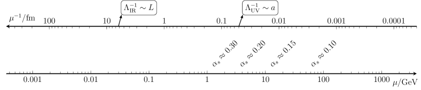
Figure 1: Lattice QCD simulations come with an IR cutoff $\Lambda_{\rm IR}=L^{-1}$ (where $L$ is the size of the finite space-time volume of the simulation), and a UV cutoff $\Lambda_{\rm UV}=a^{-1}$ (where $a$ is the lattice spacing). All relevant physical scales must lie far away from both these cutoffs in order to be free from finite-volume and discretization effects. As a result, given the current computational and algorithmic capabilities, if one wants to compute some hadronic quantities, the range of high-energy scales that can simultaneously be probed is limited.

In principle, both kind of uncertainties decrease by taking $q\to\infty$. Unfortunately, though, a single lattice simulation can only cover a limited range of energy scales (Fig. 1). Thus, if one insists on determining the hadronic scale (e.g. $m_{p}$) and the value of the observable ${O}(q)$ using the same lattice simulation, the volume has to be large, $L\gtrsim 1/m_{\pi}$, and therefore the energy scales $q$ that can be reached are at most a few GeV. Power corrections decrease quickly with the energy scale $q$, but due to the logarithmic dependence of the strong coupling with the energy scale,

$$\alpha_{S}(q)\overset{q\to\infty}{\sim}\frac{1}{\log(q/\Lambda_{\rm QCD})}\,,$$ (13)

perturbative uncertainties decrease very slowly. In fact, most lattice QCD extractions of the strong coupling are dominated by the truncation uncertainties of the perturbative series.

What can be said about such perturbative uncertainties? First, it has to be noted that due to the asymptotic nature of perturbative expansions, it is in general very difficult to estimate the difference between the truncated series for ${O}(q)$ and its nonperturbative value (see the original works DallaBrida:2018rfy ; Brida:2016flw and the review DelDebbio:2021ryq ). Second, an idea of the size of such uncertainties can be obtained by using the scale-variation method. If one assumes that at scales $q$ power corrections are negligible, one can use an arbitrary renormalization scale in the perturbative expansion Eq. (12),

$${O}(q)\overset{q\to\infty}{\sim}\alpha_{S}(\mu)+\sum_{n=2}^{N}c_{n}(\mu/q)\alpha_{S}^{n}(\mu)+{\mathcal{O}}\left(\alpha_{S}^{N+1}(\mu)\right)+\dots\,.$$ (14)

The dependence on $\mu$ on the r.h.s. is spurious, and due to the truncation of the perturbative series. This dependence can be exploited to estimate the truncation effects: the value of $\alpha_{S}$ can be extracted for different choices of $\mu$, and the differences among these extractions will give us an estimate of the truncation effects. Moreover, following Ref. DelDebbio:2021ryq , the estimate of the truncation uncertainties can be obtained from the known perturbative coefficients alone. No nonperturbative data for ${O}(q)$ is needed to estimate these uncertainties.

In Ref. DelDebbio:2021ryq a detailed analysis of several lattice methods to extract the strong coupling is performed along these lines. What are their conclusions? Most “large volume” approaches (those that aim at computing the scale $q$ in physical units and the observable ${O}(q)$ using the same lattices) have perturbative uncertainties between about $1\%$ and $3\%$ in $\alpha_{S}(m^{2}_{\mathrm{Z}})$.

It is important to emphasize that this generic approach cannot say what the errors of a specific determination are. However, given the fact that scale uncertainties can underestimate the true truncation errors (see Ref. DallaBrida:2018rfy for a concrete example), this exercise draws a clear picture: a substantial reduction in the uncertainty of the strong coupling will only come from dedicated approaches, where the multiscale problem discussed above is solved. In these proceedings, we will summarize the efforts of the ALPHA collaboration in solving this challenging problem (see refs. Sommer:2015kza ; DallaBrida:2020pag for a review).

a Finite-volume schemes

A first step towards solving the difficult multiscale problem of extracting $\alpha_{S}$ using lattice QCD comes from the following simple realization. The computation of the hadronic quantities $m_{\rm had}$, needed for fixing the bare parameters of the lattice QCD action, and the determination of the nonperturbative coupling $\alpha_{O}(q)\equiv{O}(q)$ at large $q$, from which we extract $\alpha_{S}$, are two distinct problems. Hence, in order to best keep all relevant uncertainties under control, we need dedicated lattice simulations for the calculation of $\alpha_{O}(q)$. In fact, as mentioned above, despite being convenient in practice, determinations of $\alpha_{O}(q)$ based on simulations originally intended for the computation of low-energy quantities come with severe limitations on the energy scales $q$ at which $\alpha_{S}$ can be extracted. As a concrete example, consider a typical state-of-the-art hadronic lattice simulation, with e.g. $L/a=128$ points in each of the four space-time dimensions, and a spatial size $L$ large enough to comfortably fit all the relevant low-energy physics, say, $m_{\pi}L\approx 4$ with $m_{\pi}\approx 135\,{\rm MeV}$. This results in a lattice spacing $a\approx 0.045\,{\rm fm}$, which sets the constraint, $q\ll a^{-1}\approx 4\,{\rm GeV}$. With such a low upper-limit on $q$, reaching high precision on $\alpha_{S}$ is very likely impeded by the systematic uncertainties related to perturbative truncation errors and nonperturbative corrections.

The most effective way to determine nonperturbatively the coupling $\alpha_{O}(q)$ at high-energy is to consider a finite-volume renormalization scheme Luscher:1991wu . These schemes are built in terms of observables ${O}$ defined in a finite space-time volume. The renormalization scale of the coupling $q$ is then identified with the inverse spatial size of the finite volume, i.e. $q=L^{-1}$. In order words, a running coupling is defined through the response of some correlation function(s) as the volume of the system is varied. As a result, finite volume effects are part of the definition of the coupling, rather than a systematic uncertainty in its determination. This is clearly an advantage, since for these schemes lattice systematics are under control once a single condition, $L^{-1}=q\ll a^{-1}$ $\Rightarrow$ $L/a\gg 1$, is met. This is a much simpler situation than having to simultaneously satisfy: $L^{-1}\ll q\ll a^{-1}$. In principle, there is lots of freedom in choosing a finite-volume scheme. However, in practical applications several technical aspects need to be taken intro consideration. We refer the reader to Ref. Sommer:2015kza for a detailed discussion about these points and for concrete examples of schemes.

b Step-scaling strategy

The way we exploit finite-volume schemes for the determination of $\alpha_{S}$ can be summarized in a few key steps, which we typically refer to as step-scaling strategy Luscher:1991wu ; Jansen:1995ck ; Sommer:2015kza . 1) We begin at low-energy by implicitly defining an hadronic scale $\mu_{\rm had}$ through a specific value of a chosen finite-volume coupling. Taking $\alpha_{O}(\mu_{\rm had}=L^{-1}_{\rm had})\sim 1$, we expect $\mu_{\rm had}\approx\Lambda_{\rm QCD}$. 2) Using results from hadronic, large volume simulations, we can accurately establish the value of $\mu_{\rm had}$ in physical units. This is done by computing the ratio $\mu_{\rm had}/m_{\rm had}\sim\mathcal{O}(1)$, where $m_{\rm had}$ is an experimentally measurable low-energy quantity, e.g. an hadronic mass or decay constant. 3) We simulate pairs of lattices with physical sizes $L$ and $L/2$, and determine the nonperturbative running of the finite-volume coupling $\alpha_{O}(1/L)$ with the energy scale. This is encoded in the (inverse) step-scaling function: $\sigma^{-1}_{O}(u)=\alpha_{O}(2/L)|_{u=\alpha_{O}(1/L)}$, which measures the variation of the coupling as the energy scale is increased by a factor of two. 4) Starting from $\mu_{\rm had}=L_{\rm had}^{-1}\sim\mathcal{O}(100)\,{\rm MeV}$, after $n\sim\mathcal{O}(10)$ steps as in 3), we reach nonperturbatively high-energy scales, $\mu_{\rm PT}=2^{n}/L_{\rm had}\sim\mathcal{O}(100)\,{\rm GeV}$. 5) Using the perturbative expansion of $\alpha_{O}(\mu_{\rm PT})$ in terms of $\alpha_{\overline{\mathrm{MS}}}(\mu_{\rm PT})$ we extract the latter (cf. Eq. (12)). 6) Given $\alpha_{\overline{\mathrm{MS}}}(\mu_{\rm PT})$, through the perturbative running in the $\overline{\mathrm{MS}}$-scheme, we obtain a value for $\Lambda_{\overline{\mathrm{MS}}}/\mu_{\rm PT}$, from which $\Lambda_{\overline{\mathrm{MS}}}/m_{\rm had}$ can readily be inferred.

c $\alpha_{S}$ from a nonperturbative determination of $\Lambda_{\overline{\mathrm{MS}}}^{({N_{\mathrm{f}}}=3)}$

Following a step-scaling strategy, the ALPHA collaboration has obtained a subpercent precision determination of $\alpha_{S}(m^{2}_{\mathrm{Z}})$ from a nonperturbative determination of $\Lambda_{\overline{\mathrm{MS}}}^{(3)}$ Brida:2016flw ; DallaBrida:2016kgh ; Bruno:2017gxd ; DallaBrida:2018rfy . We refer the reader to these references for the details on our previous calculation. Here we simply want to recall a few points which are relevant for the following discussion. In refs. DallaBrida:2016kgh ; DallaBrida:2018rfy the nonperturbative running of some convenient finite-volume couplings in ${N_{\mathrm{f}}}=3$ QCD was obtained, from $\mu_{\rm had}=197(3)\,{\rm MeV}$, up to $\sim$ 140 GeV. Using NNLO perturbation theory, $\alpha^{(3)}_{\overline{\mathrm{MS}}}(\mu_{\rm PT})$ was then extracted at $\mu_{\rm PT}\approx 70\,{\rm GeV}$, and from it the result: $\Lambda_{\overline{\mathrm{MS}}}^{(3)}=341(12)\,{\rm MeV}$. Thanks to the fact that we covered nonperturbatively a wide range of high-energy scales, a careful assessment of the accuracy of perturbation theory in matching the finite-volume and $\overline{\mathrm{MS}}$ schemes was possible. The result is that the error on $\Lambda_{\overline{\mathrm{MS}}}^{(3)}$ is entirely dominated by the statistical uncertainties associated with the determination of the nonperturbative running from low to high energy Bruno:2017gxd . In particular, perturbative truncation errors and nonperturbative corrections are completely negligible within the statistical uncertainties DallaBrida:2018rfy . Finally, from the result for $\Lambda_{\overline{\mathrm{MS}}}^{(3)}$, using perturbative decoupling relations, we included the effect of the charm and bottom quarks in the running to arrive at: $\alpha_{\overline{\mathrm{MS}}}^{(5)}(m_{\mathrm{Z}})=0.1185(8)$ Bruno:2017gxd . From these observations, it is clear that an improved determination of $\alpha_{S}$ may be obtained by reducing the statistical uncertainties on $\Lambda_{\overline{\mathrm{MS}}}^{(3)}$ due to the nonperturbative running of the finite-volume couplings. On the other hand, to which extent this is possible very much depends on how accurate it is to rely on perturbative decoupling for including charm effects.

d How accurate is ${N_{\mathrm{f}}}=3$ QCD?

Including the charm is particularly challenging in hadronic, large volume simulations. The charm has a mass $m_{c}\approx 1.3\,{\rm GeV}$. In units of the typical cutoffs set in hadronic simulations this means $am_{c}\gtrsim 0.3$. It is thus difficult to comfortably resolve the characteristic energy scales associated with the charm in current large volume simulations: it requires very fine lattice spacings, which are computationally very demanding. In addition, simulations become more expensive as the number of quarks increases, and the tuning of the parameters in the lattice QCD action is more involved. It is therefore important to assess whether the computational effort required to include the charm is actually needed to significantly improve our current precision on $\alpha_{S}$. If that is not the case, the resources are better invested in improving the results from ${N_{\mathrm{f}}}=3$ QCD.

In order to answer this question, we must study the systematics that enter in the $\Lambda_{\overline{\mathrm{MS}}}^{(3)}\to\Lambda_{\overline{\mathrm{MS}}}^{(4)}$ step. The first class is related to the use of perturbative decoupling relations for estimating the ratio $\Lambda_{\overline{\mathrm{MS}}}^{(3)}/\Lambda_{\overline{\mathrm{MS}}}^{(4)}$. As we shall recall below, the ratio of $\Lambda$-parameters with different flavour content is given by a function $P_{\ell,\rm f}(M/\Lambda_{\overline{\mathrm{MS}}}^{({N_{\mathrm{f}}})})=\Lambda_{\overline{\mathrm{MS}}}^{({N_{\ell}})}/\Lambda_{\overline{\mathrm{MS}}}^{({N_{\mathrm{f}}})}$, which depends on the renormalization group invariant (RGI) mass $M$ of the decoupling quark(s) and the theories considered. The function $P_{\ell,\rm f}$ can in principle be nonperturbatively defined (Sect. f). In phenomenological applications, however, we approximate it with its asymptotic, perturbative expansion at some finite loop-order, i.e. $P_{\ell,\rm f}(M/\Lambda_{\overline{\mathrm{MS}}}^{({N_{\mathrm{f}}})})\sim P_{\ell,\rm f}^{(n\text{-loop})}(M/\Lambda_{\overline{\mathrm{MS}}}^{({N_{\mathrm{f}}})})+\mathcal{O}(\alpha^{n-1}(M))+\mathcal{O}(M^{-2})$. Whether this is appropriate, it all depends on the size of the perturbative and nonperturbative corrections to this approximation for values of the quark masses $M\sim M_{c}$, with $M_{c}$ the RGI charm mass.

The second class of charm effects concerns the hadronic renormalization of the lattice theory. Normally, the bare parameters entering the lattice QCD action are tuned by requiring that a number of ratios of hadronic quantities $R_{H}$ (as many as parameters to tune), reproduce their experimental counter-parts. Typical examples are, for instance, $R_{H}=m_{\pi}/f_{\pi},m_{K}/f_{\pi},\ldots$ On the other hand, ${N_{\mathrm{f}}}=3$ QCD simulations do not include charm effects, while these are obviously present in the experimental determinations. Whether this mismatch is relevant in practice, it all depends on the actual size of charm effects in the ratios $R_{H}$.

e Effective theory of decoupling and perturbative matching

For the ease of presentation, we define our fundamental theory as ${N_{\mathrm{f}}}$-flavour QCD (${\rm QCD}_{{N_{\mathrm{f}}}}$) with ${N_{\ell}}$ massless quarks, and ${N_{\mathrm{h}}}={N_{\mathrm{f}}}-{N_{\ell}}$ mass-degenerate heavy quarks of mass $M$. In the limit where $M$ is larger than any other scale in the problem, this theory can be approximated by an effective theory (EFT) with Lagrangian Weinberg:1980wa

$$\mathcal{L}_{\rm dec}=\mathcal{L}_{\rm QCD_{N_{\ell}}}+{1\over M^{2}}\sum_{i}\omega_{i}\Phi_{i}+\mathcal{O}(M^{-4})\,.$$ (15)

The leading order term in the $1/M$ expansion is the Lagrangian $\mathcal{L}_{\rm QCD_{N_{\ell}}}$ of massless ${\rm QCD}_{{N_{\ell}}}$, while the effect of the heavy quarks is represented by non-renormalizable interactions $\Phi_{i}$ suppressed by higher powers of $1/M$. Massless ${\rm QCD}_{{N_{\ell}}}$ has a single parameter, the gauge coupling $\bar{g}^{({N_{\ell}})}$. The EFT is hence predictive once its coupling is given as a proper function of the coupling of the fundamental theory, $\bar{g}^{({N_{\mathrm{f}}})}$, and the quark masses $M$. In this situation, we say that the couplings are matched,

$$\bar{g}^{({N_{\ell}})}(\mu)=F_{O}(\bar{g}^{({N_{\mathrm{f}}})}(\mu),M/\mu)\,.$$ (16)

The function $F_{O}$ depends in principle on the observable ${O}$ that is used to establish the matching. At leading order in the EFT, however, it is consistent to drop any correction of $\mathcal{O}(M^{-2})$ in the relation (16), which thus becomes universal, i.e. it only depends on the renormalization scheme chosen for the couplings. In the $\overline{\mathrm{MS}}$-scheme, the so-called decoupling relation (16) is known at 4-loop order Bernreuther:1981sg ; Schroder:2005hy ; Chetyrkin:2005ia ; Kniehl:2006bg ; Grozin:2011nk ; Gerlach:2018hen , and it is usually evaluated at the scale $\mu=m_{\star}$, where $m_{\star}=\overline{m}_{\overline{\mathrm{MS}}}(m_{\star})$ with $\overline{m}_{\overline{\mathrm{MS}}}(\mu)$ the mass of the heavy quarks in the $\overline{\mathrm{MS}}$-scheme. In formulas,

$$\bar{g}_{\overline{\text{\rm MS}}}^{({N_{\ell}})}(m_{\star})=g_{\star}\,{\xi}\big{(}g_{\star})\,,\qquad g_{\star}\equiv\bar{g}_{\overline{\text{\rm MS}}}^{({N_{\mathrm{f}}})}(m_{\star})\,,\qquad\xi(g)=1+c_{2}g^{4}+c_{3}g^{6}+c_{4}g^{8}+\mathcal{O}(g^{10})\,.$$ (17)

The relation between the couplings can be re-expressed in terms of the corresponding $\Lambda$-parameters of the two theories,

$$P_{\ell,\rm f}(M/\Lambda_{\overline{\mathrm{MS}}}^{({N_{\mathrm{f}}})})={\Lambda_{\overline{\mathrm{MS}}}^{({N_{\ell}})}/\Lambda_{\overline{\mathrm{MS}}}^{({N_{\mathrm{f}}})}}={\varphi^{({N_{\ell}})}_{\overline{\rm MS}}\big{(}g_{\star}\,{\xi}(g_{\star})\big{)}/\varphi^{({N_{\mathrm{f}}})}_{\overline{\rm MS}}(g_{\star})}\,,$$ (18)

where the RGI-parameters are given by ${\Lambda^{({N_{\mathrm{f}}})}_{\rm X}}=\mu\,\varphi^{({N_{\mathrm{f}}})}_{\rm X}(\bar{g}^{({N_{\mathrm{f}}})}_{\rm X}(\mu))$ and $M=\overline{m}_{\rm X}(\mu)\varepsilon^{({N_{\mathrm{f}}})}_{\rm X}(\bar{g}^{({N_{\mathrm{f}}})}_{\rm X}(\mu))$. Explicit expressions for the functions $\varphi^{({N_{\mathrm{f}}})}_{\rm X}$ and $\varepsilon^{({N_{\mathrm{f}}})}_{\rm X}$ in terms of the $\beta$- and $\tau$-functions in a generic scheme ${\rm X}$ can be found in e.g. ref. Sommer:2015kza .

In Fig. 2 we present the perturbative results from Ref. Athenodorou:2018wpk for $P_{\ell,\rm f}(M/\Lambda_{\overline{\mathrm{MS}}}^{({N_{\mathrm{f}}})})$, for the phenomenological relevant cases of ${N_{\ell}}=3$, ${N_{\mathrm{f}}}=4$ and ${N_{\ell}}=4$, ${N_{\mathrm{f}}}=5$. More precisely, we show the relative deviation with respect to the 1-loop approximation, $P^{(1)}_{\ell,\rm f}$, for different orders of the perturbative expansion of $P_{\ell,\rm f}$. Focusing on the case of $P_{3,4}$, we see how the perturbative corrections at 4- and 5-loop order are very small already for values of $M$ comparable to that of the charm. Judging from the perturbative behavior alone, the series thus appears to be well within its regime of applicability. As a result, any estimate for the perturbative truncation errors on $P_{\ell,\rm f}$ based on the last-known contributions to the series leads to very small uncertainties. When translated to the coupling we find, for instance, $\alpha^{(5)}_{\overline{\text{\rm MS}}}(m_{\mathrm{Z}})=0.1185(8)(3)_{\rm PTdec}$, where the second error is estimated as the sum of the full 4- and 5-loop contributions due to the decoupling of both charm and bottom quarks Bruno:2017gxd . As anticipated, the perturbative error estimate is well-below the uncertainties from other sources.

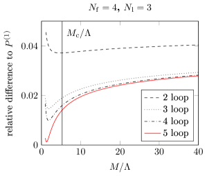
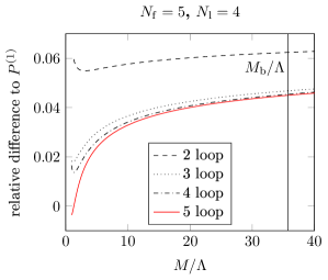
Figure 2: Relative differences from the (unsystematic) 1-loop approximation $P^{(1)}_{\ell,\rm f}(M/\Lambda)=(M/\Lambda)^{\eta_{0}}$, $\eta_{0}=2{N_{\mathrm{h}}}/(33-2{N_{\ell}})$, for different orders of the perturbative expansion of $P_{\ell,\rm f}(M/\Lambda)$ as a function of $M/\Lambda$ Athenodorou:2018wpk . The results for ${N_{\ell}}=3$, ${N_{\mathrm{f}}}=4$ (${N_{\ell}}=4$, ${N_{\mathrm{f}}}=5$) are given in the left (right) panel. The values for the RGI charm ($M_{c}$) and bottom ($M_{b}$) quark masses in units of the proper $\Lambda$-parameters are marked by vertical lines.

f How perturbative are heavy quarks?

Above we have shown how within perturbation theory, the perturbative decoupling of the charm appears to be very accurate. A natural question to ask at this point is how reliable this picture is at the nonperturbative level. In other words, can we quantify the accuracy of perturbative decoupling for the charm by comparing it directly to nonperturbative results, thus getting an estimate for the size of nonperturbative corrections? In order to answer this question, we start by formulating the matching of $\Lambda$-parameters (18) in nonperturbative terms Bruno:2014ufa ; Athenodorou:2018wpk ,

$${\Lambda^{({N_{\ell}})}_{\overline{\mathrm{MS}}}\over m_{\rm had,1}^{({N_{\ell}})}}=P^{\rm had,1}_{\ell,\rm f}\big{(}{M/\Lambda^{({N_{\mathrm{f}}})}_{\overline{\mathrm{MS}}}}\big{)}{\Lambda^{({N_{\mathrm{f}}})}_{\overline{\mathrm{MS}}}\over m_{\rm had,1}^{({N_{\mathrm{f}}})}(M)}\,.$$ (19)

We thus say that the EFT is matched to the fundamental theory if its $\Lambda$-parameter $\Lambda^{({N_{\ell}})}_{\overline{\mathrm{MS}}}\equiv\Lambda^{({N_{\ell}})}_{\overline{\mathrm{MS}}}(M,\Lambda^{({N_{\mathrm{f}}})}_{\overline{\mathrm{MS}}})$ in units of an hadronic quantity $m_{\rm had,1}^{({N_{\ell}})}$, is a proper function of the heavy quark masses $M$, and the $\Lambda$-parameter of the fundamental theory $\Lambda^{({N_{\mathrm{f}}})}_{\overline{\mathrm{MS}}}$ in units of the same hadronic quantity $m_{\rm had,1}^{({N_{\mathrm{f}}})}(M)$, computed in ${\rm QCD}_{{N_{\mathrm{f}}}}$ where ${N_{\mathrm{h}}}$ quarks are heavy with mass $M\gg\Lambda_{\rm QCD}$. Once the theories are matched, decoupling predicts that for any other hadronic quantity $m_{\rm had,2}^{({N_{\ell}})}$ computed in the EFT, we should expect: $m_{\rm had,2}^{({N_{\ell}})}=m_{\rm had,2}^{({N_{\mathrm{f}}})}(M)+\mathcal{O}(M^{-2})$ (cf. Sect. e). As anticipated by our notation, the function $P^{\rm had}_{\ell,\rm f}$ depends on the hadronic quantity considered for the matching. If we were to choose a different quantity, we expect: $P^{\rm had,1}_{\ell,\rm f}\big{(}{M/\Lambda^{({N_{\mathrm{f}}})}_{\overline{\mathrm{MS}}}}\big{)}\sim P^{\rm had,2}_{\ell,\rm f}\big{(}{M/\Lambda^{({N_{\mathrm{f}}})}_{\overline{\mathrm{MS}}}}\big{)}+\mathcal{O}(M^{-2})$.

The relation (19) leads to the interesting factorization formula Bruno:2014ufa ; Athenodorou:2018wpk ,

$${m_{\rm had}^{({N_{\mathrm{f}}})}(M)\over m_{\rm had}^{({N_{\mathrm{f}}})}(0)}={Q}^{\rm had}_{\ell,\rm f}\times P^{\rm had}_{\ell,\rm f}\big{(}{M/\Lambda^{({N_{\mathrm{f}}})}_{\overline{\mathrm{MS}}}}\big{)}\,,\qquad{Q}^{\rm had}_{\ell,\rm f}={m_{\rm had}^{({N_{\ell}})}/\Lambda^{({N_{\ell}})}_{\overline{\mathrm{MS}}}\over m_{\rm had}^{({N_{\mathrm{f}}})}(0)/\Lambda^{({N_{\mathrm{f}}})}_{\overline{\mathrm{MS}}}}\,.$$ (20)

On the l.h.s. of this equation we have the hadronic quantity $m_{\rm had}^{({N_{\mathrm{f}}})}(M)$ computed in ${\rm QCD}_{{N_{\mathrm{f}}}}$ where ${N_{\mathrm{h}}}$ quarks have mass $M$, over the same hadronic quantity $m_{\rm had}^{({N_{\mathrm{f}}})}(0)$ computed in the chiral limit, i.e. where all ${N_{\mathrm{f}}}$ quarks are massless. This ratio can be expressed as the product of a nonperturbative, $M$-independent factor $Q^{\rm had}_{\ell,\rm f}$, and the function $P^{\rm had}_{\ell,\rm f}\big{(}{M/\Lambda^{({N_{\mathrm{f}}})}_{\overline{\mathrm{MS}}}}\big{)}$, which encodes all the $M$-dependence. As we recalled in Sect. e, for $M\to\infty$ the function $P^{\rm had}_{\ell,\rm f}$ admits an asymptotic perturbative expansion. Hence, by measuring nonperturbatively on the lattice the l.h.s. of Eq. (20), we can compare the $M$-dependence of several such ratios with what is predicted by a perturbative approximation for $P^{\rm had}_{\ell,\rm f}$. In this way, we can assess the typical size of nonperturbative effects in $P^{\rm had}_{\ell,\rm f}$ as a function of $M$. In Ref. Athenodorou:2018wpk a careful study was carried out considering the case of the decoupling of two heavy quarks with mass $M\sim M_{c}$, for the case of ${N_{\ell}}=0$, ${N_{\mathrm{f}}}=2$. Under very reasonable assumptions, it is possible to extract from these results quantitative information on the nonperturbative corrections in the phenomenological interesting case of $P_{3,4}(M_{c}/\Lambda^{(4)}_{\overline{\mathrm{MS}}})$. The conclusions of Ref. Athenodorou:2018wpk are that these effects are very much likely below the per-cent level. This means that it is safe to use a perturbative estimate for $P_{3,4}(M_{c}/\Lambda^{(4)}_{\overline{\mathrm{MS}}})$ in transitioning from $\Lambda_{\overline{\mathrm{MS}}}^{(3)}\to\Lambda_{\overline{\mathrm{MS}}}^{(4)}$, as long as, say, $\delta\Lambda_{\overline{\mathrm{MS}}}^{(3)}\gtrsim 1.5\%$ or so.

If we now consider ratios of hadronic quantities, where the dependence on the $\Lambda$-parameters drops out, we immediately conclude that

$${m_{\rm had,1}^{({N_{\ell}})}/m_{\rm had,2}^{({N_{\ell}})}}={m_{\rm had,1}^{({N_{\mathrm{f}}})}(M)/m_{\rm had,2}^{({N_{\mathrm{f}}})}(M)}+{\mathcal{O}}(M^{-2})\,.$$ (21)

In this case, one can obtain estimates for the typically size of $\mathcal{O}(M^{-2})$ effects in these ratios by comparing both sides of the above equation computed through lattice simulations. In refs. Knechtli:2017xgy ; Hollwieser:2020qri careful studies have been conducted considering both the case of the decoupling of two heavy quarks of mass $M\sim M_{c}$ with ${N_{\ell}}=0$, ${N_{\mathrm{f}}}=2$, and more recently for the decoupling of a single charm quark with ${N_{\ell}}=3$, ${N_{\mathrm{f}}}=3+1$, i.e. in the presence of three mass-degenerate lighter quarks. From these calculations, the authors conclude that the typical effects due to the charm on dimensionless ratios of low-energy quantities are well-below the per-cent level. This means that these effects are not relevant for a per-cent precision determinations of $\Lambda_{\overline{\mathrm{MS}}}^{(3)}$.

In summary, thanks to recent dedicated studies, we are able to conclude that it is safe to rely on perturbative decoupling for the charm quark in connecting $\Lambda_{\overline{\mathrm{MS}}}^{(3)}$ and $\Lambda_{\overline{\mathrm{MS}}}^{(4)}$, as long as $\delta\Lambda_{\overline{\mathrm{MS}}}^{(3)}\gtrsim 1.5\%$. The 0.7% precision extraction of $\alpha_{S}$ from Ref. Bruno:2017gxd is based on a determination of $\Lambda_{\overline{\mathrm{MS}}}^{(3)}$ with an uncertainty of $\delta\Lambda_{\overline{\mathrm{MS}}}^{(3)}\approx 3.5\%$ (cf. Sec. c). Hence, there is still about a factor of two of possible improvement within the ${N_{\mathrm{f}}}=3$ flavour theory.

g The strong coupling from the decoupling of heavy quarks

The previous section suggests a method to relate the $\Lambda$-parameters in theories with a different number of quark flavors (cf. Eq. (19)). Taking this relation to the extreme, one should be able to determine $\Lambda_{\overline{\rm MS}}^{(N_{\rm f})}$ from the pure-gauge one, $\Lambda_{\overline{\rm MS}}^{(0)}$. Of course this requires to decouple $N_{\rm f}$ heavy quarks with $M\gg\Lambda^{(N_{\rm f})}_{\overline{\rm MS}}$. The physical world is very different from this limit, but lattice QCD can simulate such unphysical situation.

A possible strategy for the determination of the strong coupling based on this idea is the following:

1. Starting from a scale $\mu_{\rm dec}$ in ${\rm QCD}_{N_{\rm f}}$, one determines the value of a nonperturbatively defined coupling at such scale in a massless renormalization scheme, $\bar{g}^{(N_{\rm f})}_{{O}}(\mu_{\rm dec})$.

2. By performing lattice simulations at increasing values of the quark masses, one is able to determine the value of the coupling in a massive scheme, $\bar{g}^{(N_{\rm f})}_{{O}}(\mu_{\rm dec},M)$.

3. For $M$ larger than any other scale in the problem (i.e. $M\gg\Lambda_{\rm QCD},\mu_{\rm dec}$), the massive coupling is, up to heavy-mass corrections, the same as the corresponding coupling in the pure-gauge theory, i.e.

   $$\bar{g}^{(N_{\rm f})}_{{O}}(\mu_{\rm dec},M)=\bar{g}^{(0)}_{{O}}(\mu_{\rm dec})\,,$$ (22)

   where corrections of $\mathcal{O}(1/M^{2})$ have been dropped.

4. From the running of the coupling $\bar{g}^{(0)}_{{O}}(\mu_{\rm dec})$ in the pure-gauge theory we can determine the pure-gauge $\Lambda$-parameter in units of $\mu_{\rm dec}$,

   $$\frac{\Lambda^{(0)}_{\overline{\rm MS}}}{\mu_{\rm dec}}=\frac{\Lambda^{(0)}_{\overline{\rm MS}}}{\Lambda^{(0)}_{{O}}}\times\varphi^{(0)}_{{O}}(\bar{g}^{(0)}_{{O}}(\mu_{\rm dec}))\,.$$ (23)

   (Note that the ratio of $\Lambda$-parameters in different schemes can be exactly determined via a perturbative, 1-loop computation (cf. e.g. ref. Sommer:2015kza ).)

5. Since all $N_{\rm f}$ quarks are heavy, one can employ the decoupling relations to estimate the ${N_{\mathrm{f}}}\geq 3$ flavor $\Lambda$-parameter as (cf. Eq. (19)),

   $$\Lambda^{(N_{\rm f})}_{\overline{\rm MS}}=\mu_{\rm dec}\times\frac{\Lambda^{(0)}_{\overline{\rm MS}}}{\Lambda^{(0)}_{{O}}}\times\varphi^{(0)}_{{O}}(\bar{g}^{(0)}_{{O}}(\mu_{\rm dec}))\times\frac{1}{P^{(5\text{-loop})}_{0,N_{\rm f}}(M/\Lambda^{(N_{\rm f})}_{\overline{\rm MS}})}+\mathcal{O}(\alpha_{S}^{4}(m_{\star}))+\mathcal{O}(M^{-2})\,.$$ (24)

Equation (24) is our master formula to determine $\Lambda^{(N_{\rm f}=3)}_{\overline{\rm MS}}$ from precise results for the nonperturbative running of the gauge coupling in the pure-gauge theory (i.e. for the function $\varphi^{(0)}_{O}$). Several comments are in order at this point:

• There are two types of corrections in Eq. (24). First, “perturbative” ones of $\mathcal{O}(\alpha_{S}^{4}(m_{\star}))$. They come from using perturbation theory for the function $P_{0,N_{\rm f}}$. Second, we have nonperturbative “power” corrections. Their origin is the decoupling condition, Eq. (22), as well as the use of a perturbative approximation for the function $P_{0,N_{\rm f}}$.

• Both perturbative and power corrections vanish for $M\to\infty$. In fact, the following relation is exact

  $$\Lambda^{(N_{\rm f})}_{\overline{\rm MS}}=\lim_{M\to\infty}\mu_{\rm dec}\times\frac{\Lambda^{(0)}_{\overline{\rm MS}}}{\Lambda^{(0)}_{{O}}}\times\varphi^{(0)}_{{O}}(\bar{g}^{(0)}_{{O}}(\mu_{\rm dec}))\times\frac{1}{P^{(n\text{-loop})}_{0,N_{\rm f}}(M/\Lambda^{(N_{\rm f})}_{\overline{\rm MS}})}\,,$$ (25)

  with $\bar{g}^{(0)}_{{O}}(\mu_{\rm dec})=\bar{g}^{(N_{\rm f})}_{{O}}(\mu_{\rm dec},M)$.

• The situation and challenges in this approach might look similar to those present in more “conventional” extractions of the strong coupling (cf. Eq. (12)). The subtle difference however is that, in the present case, perturbative corrections are very small even for scales $\sim M_{c}$ (cf. Sect. e). In particular, if one is considering quarks with masses of a few GeV, they are completely negligible in practice, and one has only to deal with the power corrections, which decrease much faster with the relevant energy scale.

This method to extract the strong coupling was proposed in Ref. DallaBrida:2019mqg (for a recent review see Ref. DallaBrida:2020pag ). Here we present preliminary results using this strategy Brida:2021xwa . We follow closely the strategy described above, skipping the technical details. The reader interested in the details is encouraged to look at the original references DallaBrida:2019mqg ; DallaBrida:2020pag ; Brida:2021xwa .

1. A scale $\mu_{\rm dec}=789(15)$ MeV is determined in a finite-volume renormalization scheme in three-flavor QCD using results from Ref. DallaBrida:2016kgh . This corresponds to a value of the renormalized nonperturbative coupling $\bar{g}^{(3)}(\mu_{\rm dec})\approx 1.9872$.

2. For technical reasons the massive coupling is determined in a slightly different renormalization scheme than the massless one. The value of the massive coupling is then determined by keeping the value of the bare coupling (and therefore the lattice spacing) fixed and increasing the value of the quark masses. This determination is performed for several values of the quark masses, $z=M/\mu_{\rm dec}=1.972,4,6,8,12$, and several values of the lattice spacing with $1/(a\mu_{\rm dec})=12,\dots,40$. The results are extrapolated to the continuum limit for each value of the quark masses labeled by $z$ (Figs. 3).

   

   

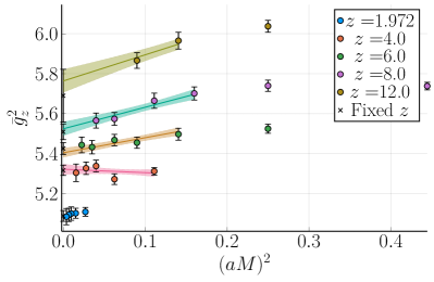
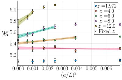
   Figure 3: Continuum extrapolations of the massive coupling $\bar{g}^{2}_{z}=[\bar{g}^{(3)}(\mu_{\rm dec},M)]^{2}$ for different values of the quark masses labeled by $z=M/\mu_{\rm dec}$. Only data at fine enough lattice spacings (i.e. for which ($aM)^{2}<0.16$) are included in the fit.

3. The values of the massive coupling are used as matching condition between ${\rm QCD}_{N_{\rm f}}$ and the pure-gauge theory (cf. Eq. (22)). The running in the pure-gauge theory is known very precisely from the literature DallaBrida:2019wur . The ratio ${\Lambda^{(0)}_{\overline{\rm MS}}}/{\mu_{\rm dec}}$ can thus be accurately determined.

   Table 2: Values of the massive three-flavor coupling $\bar{g}^{(3)}(\mu_{\rm dec})$ and the corresponding values of $\Lambda^{(3)}_{\overline{\rm MS}}$ obtained by applying our master formula Eq.. (24) and ignoring perturbative and power corrections.

   $z$	$[\bar{g}^{(3)}(\mu_{\rm dec})]^{2}$	$\Lambda^{(3)}_{\overline{\rm MS}}$ [MeV]
   4	5.322(26)	389(11)
   6	5.404(23)	362(10)
   8	5.524(35)	350(10)
   12	5.764(58)	339(10)

4. Given this result, by applying the master formula Eq. (24), one obtains the estimates for $\Lambda^{(3)}_{\overline{\rm MS}}$ given in Table 2. These estimates should approach the correct three-flavor $\Lambda$-parameter in the limit $M\to\infty$. Figure 4 shows that this is indeed the case. Or data is consistent with a linear extrapolation in $\mu_{\rm dec}^{2}/M^{2}$, which results in

   $$\Lambda^{(3)}_{\overline{\rm MS}}=332(10)(2)\,{\rm MeV}\,,$$ (26)

   where the first uncertainty is statistical, while the second is due to different parameterizations of the $M\to\infty$ limit.

   

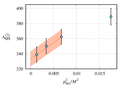
   Figure 4: Estimates of the three-flavor $\Lambda$-parameter (Table 2) and its $M\to\infty$ extrapolation yielding our final result for $\Lambda^{(3)}_{\overline{\rm MS}}$.

This result for the three-flavor $\Lambda$-parameter translates, after crossing the charm and bottom thresholds, into

$$\alpha_{S}(m^{2}_{\mathrm{Z}})=0.1179(7)\,.$$ (27)

The result has a 0.6% uncertainty, which is in fact dominated by the uncertainty on the scale $\mu_{\rm dec}=789(15)$ MeV, and by our knowledge of the running in the pure-gauge theory. Both sources of uncertainty are statistical in nature and can be reduced with a modest computational effort. The effects of the truncation of the perturbative series are subdominant in our approach. We thus conclude that a further reduction of the uncertainty by a factor of two is possible with this approach. Going beyond this precision would require including charm effects nonperturbatively and also some serious thinking on how to include electromagnetic effects in the determination of both the scale and the running.

4 Strong coupling constant $\alpha_{S}$ from moments of quarkonium correlators

A lattice method conceptually similar to the determination of $\alpha_{S}(m^{2}_{\mathrm{Z}})$ or heavy-quark masses from the $R$-ratio via quarkonium sum rules Dehnadi:2015fra ; Boito:2020lyp uses heavy-quark two-point correlators; for a recent review see Ref. Komijani:2020kst . Renormalization group invariant pseudo-scalar correlators $G(t)$ and their $n$th time moments $G_{n}$ are defined as

$$G_{n}=\sum_{t}t^{n}(G(t)+G(N_{t}-t)),\quad G(t)=a^{6}\sum_{\bm{x}}(am_{h0})^{2}\braket{j_{5}(\bm{x},t)j_{5}(0,0)},\quad j_{5}(\bm{x},t)=\bar{\psi}(\bm{x},t)\gamma_{5}\psi(\bm{x},t).$$ (28)

The symmetrization accounts for (anti-)periodic boundary conditions in time. $am_{h0}$ is the corresponding bare heavy-quark mass in the lattice scheme; $am_{h0}$ resp. $m_{h}$ can be varied quite liberally for valence quarks in the charm- and bottom-quark regions and in between. Since sea quark mass variation is expensive, most results have partially quenched heavy quarks, i.e. heavy-quark masses in sea and valence sectors can be different in (2+1+1)-flavor QCD, or heavy quarks are left out from the sea in (2+1)-flavor QCD.

The weak-coupling series of $G_{n}$, which are finite for $n\geq 4$, is known up to $\mathrm{N^{3}LO}$ resp. $\mathcal{O}(\alpha_{S}^{3}(\nu_{h}))$ for $N_{f}$ massless and one massive quark flavor Sturm:2008eb ; Kiyo:2009gb ; Maier:2009fz ,

$$G_{n}=\tfrac{g_{n}(\alpha_{S}(\nu),\nu/m_{h})}{am_{h}^{n-4}(\nu_{m})},$$ (29)

where $\nu=xm_{h}$, proportional to the heavy-quark mass $m_{h}$, is the $\mathrm{\overline{\mathrm{MS}}}$ renormalization scale of the coupling. $\nu_{m}=x_{m}m_{h}$, the scale at which the $\mathrm{\overline{\mathrm{MS}}}$ heavy-quark mass $m_{h}(\nu_{m})$ is defined, could be different from $\nu$ Dehnadi:2015fra . In published weak-coupling results, heavy-quark masses on internal (sea) and external (valence) quark lines must agree Sturm:2008eb ; Kiyo:2009gb ; Maier:2009fz . This restriction has profound implications for $\alpha_{S}$ extractions in (2+1+1)-flavor QCD.

As the bare heavy-quark mass in lattice units, $am_{h0}$, is a large parameter, improved quark actions are needed; so far most calculations have employed the highly improved staggered quarks (HISQ) HPQCD:2008kxl ; McNeile:2010ji ; Chakraborty:2014aca ; Maezawa:2016vgv ; Petreczky:2019ozv ; Petreczky:2020tky , while domain-wall fermions have been used as well Nakayama:2016atf . Some data sets involved values of $am_{h0}$ corresponding to different heavy-quark masses $m_{h}$ McNeile:2010ji ; Chakraborty:2014aca ; Petreczky:2019ozv ; Petreczky:2020tky ; for this reason even (2+1+1)-flavor QCD lattice results still involve partially quenched heavy quarks Chakraborty:2014aca . Enforcing an upper bound $am_{h0}\lesssim 1$ to limit the size of lattice artifacts implies that fewer independent ensembles can constrain the data at larger $m_{h}$ and entail larger errors of the respective continuum limit.

The so-called (tree-level) reduced moments, known perturbatively at $\mathcal{O}(\alpha_{S}^{3}(\nu_{h}))$,

$$R_{4}=\left(\tfrac{G_{4}^{\mathrm{QCD}}}{G_{4}^{\mathrm{0}}}\right)\hskip 20.00003pt, R_{4}(\alpha_{S}(\nu),\tfrac{\nu}{m_{h}})=1+\sum_{j=1}^{3}r_{nj}(\tfrac{\nu}{m_{h}})\left(\tfrac{\alpha_{S}(\nu)}{\pi}\right)^{j}$$ (30)

$$R_{n}=\left(\tfrac{G_{n}^{\mathrm{QCD}}}{G_{n}^{\mathrm{0}}}\right)^{\frac{1}{(n-4)}}, R_{n}(\alpha_{S}(\nu),\tfrac{\nu}{m_{h}})=\left(\tfrac{m_{h0}}{m_{h}(\nu_{m})}\right)\left(1+\sum_{j=1}^{3}r_{nj}(\tfrac{\nu}{m_{h}})\left(\tfrac{\alpha_{S}(\nu)}{\pi}\right)^{j}\right),~{}n>4,$$ (31)

eliminate the tree-level contribution, thus cancelling the leading lattice artifacts HPQCD:2008kxl . The coefficients $r_{nj}$ are numbers of order $1$ without any obvious pattern, see, e.g.  Table 1 of Ref. Komijani:2020kst . On the one hand, the lowest reduced moment $R_{4}$ and ratios of higher reduced moments, i.e. $\nicefrac{{R_{6}}}{{R_{8}}}$ or $\nicefrac{{R_{8}}}{{R_{10}}}$, are dimensionless; their respective continuum extrapolations turned out to be challenging, in particular due to $\log(a\Lambda_{\mathrm{QCD}})$ and $\log(am_{h0})$ dependence Petreczky:2020tky . Such $\log(a)$ dependence is manifest in slopes that decrease for larger $am_{h0}$. On the other hand, higher moments $\nicefrac{{R_{n}}}{{m_{h0}}},~{}n\geq 6$, are dimensionful and scale with $\nicefrac{{1}}{{m_{h0}}}=\nicefrac{{a}}{{(am_{h0})}}$; thus, because the scale uncertainty and the uncertainty of the tuned bare heavy-quark mass ($am_{h0}$) strongly impact the results, these are insensitive to any $\log(a)$ effects, and continuum extrapolations are straightforward. For the improved actions used in published results, lattice spacing dependence could be parameterized for functions of the reduced moments, i.e. $R(m_{h})=\{R_{4}(m_{h}),\nicefrac{{R_{n}(m_{h})}}{{m_{h0}}},\nicefrac{{R_{n}(m_{h})}}{{R_{n+2}(m_{h})}},\},~{}n\geq 6$, as

$$R(m_{h}) =R^{\mathrm{cont}}(m_{h})+\sum_{i=1}^{N}\sum_{j=1}^{M_{i}}b_{ij}^{(R)}(\alpha_{S}^{b})^{i}\Bigl{[}1+\sum_{k=1}^{i}d_{ijk}^{(R)}\ln^{k}(am_{h0})\Bigr{]}(am_{h0})^{2j},$$ (32)

where $\alpha_{S}^{b}=\nicefrac{{g_{0}^{2}}}{{(4\pi u_{0}^{4})}}$ is the boosted lattice coupling Lepage:1992xa ; the tadpole factor $u_{0}$ is defined in terms of the plaquette, $u_{0}^{4}=\braket{\nicefrac{{\mathrm{Tr}~{}{U_{\mu\nu}}}}{{N_{c}}}}$, and partially accounts for the expected $\log(a\Lambda_{\mathrm{QCD}})$ dependence.

For $R_{4}$ and $\nicefrac{{R_{6}}}{{R_{8}}}$, separate continuum extrapolations for each heavy-quark mass proved feasible only for $m_{h}\leq 1.5m_{c}$ Petreczky:2019ozv . Continuum extrapolation for $m_{h}\geq 2m_{c}$ required joint fits including $m_{h}<2m_{c}$ Petreczky:2020tky ; similar joint fits with Bayesian priors were used in Refs. McNeile:2010ji ; Chakraborty:2014aca . The published continuum results for $R_{4}$ and $\nicefrac{{R_{6}}}{{R_{8}}}$ at $m_{h}=m_{c}$ or $1.5m_{c}$ are consistent among each other Komijani:2020kst ; Petreczky:2020tky ; any significant deviations can be traced back to known deficiencies in the respective analyses Maezawa:2016vgv ; Nakayama:2016atf , see e.g. Table 65 of Ref. Aoki:2021kgd . For $\nicefrac{{R_{n}}}{{m_{h0}}},~{}n\geq 6$ fits with $N=1,~{}M_{1}=2$ are sufficient for any $m_{h}$, and published results for $R_{n}(m_{c})/m_{c0},~{}n\geq 6$ are consistent. Severe finite volume effects affect $\nicefrac{{R_{8}}}{{R_{10}}}$; $\nicefrac{{R_{8}}}{{R_{10}}}$ at $m_{c}$ is systematically low (and inconsistent with $R_{4}$), while continuum extrapolation with joint fits proved reliable for $m_{h}\geq 1.5m_{c}$ Petreczky:2020tky . With the aforementioned exceptions the continuum results in (2+1)-flavor QCD span the region $m_{h}=m_{c},\ldots,4m_{c}$ for valence quarks, see Tables 1 and 4 of Ref. Petreczky:2020tky ; with increasing heavy-quark mass $m_{h}$, $R_{4}$ and the ratios decrease towards $1$, while the errors of the lattice calculations increase. Continuum results in (2+1+1)-flavor QCD have not been published.

Comparing $R_{4}(m_{h})$ to $R_{4}(\alpha_{S}(\nu),\nicefrac{{\nu}}{{m_{h}}})$ permits extraction of $\alpha_{S}(\nu)$; truncation errors, estimated via inclusion of terms $\pm 5r_{n3}\,\alpha_{S}^{4}(\nu)$, turn out to be too large for the ratios to provide more than a cross-check Petreczky:2020tky . Once $\alpha_{S}(\nu)$ is given, $R_{n}/m_{h0}$ permits obtaining the $\overline{\mathrm{MS}}$ heavy-quark mass $m_{h}(\nu_{m})$; combining both yields $\Lambda_{\overline{\mathrm{MS}}}^{(N_{f})}$. Whether or not the two scales $\nu_{h}=xm_{h}$ and $\nu_{m}=x_{m}m_{h}$, should be varied jointly ($x=x_{m}$) or independently ($x\neq x_{m}$) is under investigation; the latter has yielded in a reanalysis of published lattice results at $m_{h}=m_{c}$ about 50% larger estimates of truncation errors Boito:2020lyp . $\alpha_{S}(\nu)$ or $m_{h}(\nu_{m})$ for different $am_{h0}=x_{\mathrm{lat}}am_{c0}$ are consistent with perturbative running Petreczky:2020tky . Nonperturbative contributions —parametrized in terms of QCD condensates— are negligible for $m_{h}\geq 1.5m_{c}$ due to suppression by powers of at least $1/m_{h}^{4}$; similarly, truncation errors diminish dramatically for $m_{h}\geq 1.5m_{c}$ Petreczky:2020tky .

Table 3: $\Lambda_{\overline{\mathrm{MS}}}^{(N_{f}=3)}$ obtained for different values of $m_{h}$ and different choices of the renormalization scale $\nu$ (using $\nu=\nu_{m}$). The first error comes from the lattice calculations, the second error is the perturbative error, and the last error is due to the gluon condensate. From Ref. Petreczky:2020tky .

$\nicefrac{{m_{h}}}{{m_{c}}}$	$\nicefrac{{\nu}}{{m_{h}}}=\nicefrac{{2}}{{3}}$	$\nicefrac{{\nu}}{{m_{h}}}=1$	$\nicefrac{{\nu}}{{m_{h}}}=\nicefrac{{3}}{{2}}$	$\nicefrac{{\nu}}{{m_{h}}}=2$	$\nicefrac{{\nu}}{{m_{h}}}=3$
1.0	–	323(4)(6)(3)	323(4)(7)(3)	327(4)(13)(3)	340(4)(21)(3)
1.5	314(8)(23)(1)	326(9)(4)(1)	326(8)(5)(1)	329(8)(10)(1)	341(9)(18)(1)
2.0	–	327(13)(3)(0)	327(13)(4)(0)	330(13)(9)(0)	341(14)(16)(0)
3.0	325(20)(20)(0)	332(21)(2)(0)	332(21)(4)(0)	335(22)(22)(0)	344(22)(14)(0)
4.0	–	336(26)(2)(0)	336(26)(3)(0)	339(27)(7)(0)	347(28)(17)(0)

A recent analysis has exposed that the choice of the lattice scale ratio, i.e. $x_{\mathrm{lat}}=\nicefrac{{m_{h}}}{{m_{c}}}=\nicefrac{{(am_{h0})}}{{(am_{c0})}}$, and the perturbative scale ratio, $x_{\mathrm{pert}}=\nicefrac{{\nu}}{{m_{h}}}$, both have a significant and systematic impact on the extracted $\Lambda_{\overline{\mathrm{MS}}}^{(N_{f})}$, and consequently on $\alpha_{S}(m^{2}_{\mathrm{Z}})$ Petreczky:2020tky , while the composition of the error budget is very different, see Table 3. Neglecting the spread due to varying either of these two scale ratios led in most past determinations to significantly underestimated errors HPQCD:2008kxl ; McNeile:2010ji ; Chakraborty:2014aca ; Maezawa:2016vgv ; Petreczky:2019ozv . Nonetheless, the central value of Ref. McNeile:2010ji is in good agreement with the corresponding entry of Table 3.

The current FLAG sub-average —taking the latest results Petreczky:2020tky partially into account, and using error estimates from independent scale variation Boito:2020lyp — reports

$$\alpha_{S}(m^{2}_{\mathrm{Z}})=0.11826(200) \text{(FLAG sub-average for heavy-quark two-point correlators)~{}\cite[cite]{\@@bibref{Authors Phrase1YearPhrase2}{Aoki:2021kgd}{\@@citephrase{(}}{\@@citephrase{)}}}}.$$ (33)

Table 3 suggests that a viable approach on the lattice side to reducing the errors in the next decade may be by performing more accurate lattice calculations using masses $m_{h}\geq 2m_{c}$, where the truncation errors are subleading in current results. The corresponding continuum extrapolations could be made more robust in two ways. First, by including more intermediate heavy-quark mass values (e.g. $\nicefrac{{m_{h}}}{{m_{c}}}=1.75,~{}2.25,~{}2.5,~{}2.75,~{}3.25$, etc.) in the joint fits, Eq. (32), one may hope to significantly reduce the lattice errors of the continuum results for $m_{h}\geq 2m_{c}$. Second, by relying on one-loop instead of tree-level reduced moments at finite lattice spacing as suggested in Ref. Weber:2020gfh , one may simplify the approach to the continuum limit; while cumbersome, these calculations in lattice perturbation theory are in principle straightforward and are expected to eliminate all $i=1$ terms from the series corresponding to Eq. (32). The availability of lattice results in (2+1+1)-flavor QCD with partially quenched heavy quarks suggests that a viable approach on the perturbative side to reducing the errors may be to permit partially quenched heavy quarks, i.e. different heavy-quark masses on internal (sea) and external (valence) lines. In particular, application of this method in (2+1+1)-flavor QCD permits no $\alpha_{S}$ extraction for valence quarks at $m_{h}>m_{c}$, the only readily available strategy to alleviate the truncation error, on the basis of the currently available weak-coupling calculations that require $m_{\text{h,sea}}=m_{\text{h,val}}$. If this deficiency were remedied, the constraining power could be improved in a joint analysis of partially quenched lattice calculations with different $m_{h}$ in (2+1+1)-flavor QCD similar to the recent analysis in (2+1)-flavor QCD Petreczky:2020tky , or by even combining (2+1)- and (2+1+1)-flavor QCD continuum results in a joint analysis that assumes perturbative decoupling of the heavy quark. Last but not least, the expected accuracy would obviously benefit from $\mathrm{N^{4}LO}$ resp. $\mathcal{O}(\alpha_{S}^{4}(\nu_{h}))$ calculations.

Acknowledgments— PP was supported by U.S. Department of Energy under Contract No. DE-SC0012704. JHW’s reserch was funded by the Deutsche Forschungsgemeinschaft (DFG, German Research Foundation) - Projektnummer 417533893/GRK2575 “Rethinking Quantum Field Theory”.

5 Strong coupling constant $\alpha_{S}$ from the static energy, the free energy and the force

QCD observables that have been computed with high precision in perturbative- and lattice-QCD with 2+1 or 2+1+1 flavors are well suited to provide determinations of $\alpha_{S}$ in the kinematic regions where pQCD applies. The advantage of looking at observables is that continuum analytical and lattice results may be compared without having to deal with renormalization issues and change of scheme. Moreover, if in the kinematic regions where pQCD is used the perturbative series converges well, and nonperturbative corrections turn out to be small, and if lattice data can be extrapolated to continuum, then a very precise extraction of $\alpha_{S}$ is possible even by comparing few lattice data with the perturbative expression. The comparison provides $\Lambda_{\overline{\mathrm{MS}}}$ times the lattice scale. By supplying a precise determination of the lattice scale, one obtains $\Lambda_{\overline{\mathrm{MS}}}$. Finally, $\Lambda_{\overline{\mathrm{MS}}}$ may be traded with $\alpha_{S}$ conventionally expressed at the mass of the Z, $\alpha_{S}(m^{2}_{\mathrm{Z}})$.

a The QCD static energy

The QCD static energy $E_{0}(r)$, i.e. the energy between a static quark and a static antiquark separated by a distance $r$, is one of these golden observables for the extraction of $\alpha_{S}$ and it is also a basic object to study the strong interactions Wilson:1974sk . The QCD static energy, $E_{0}(r)$, is defined (in Minkowski spacetime) as

$$E_{0}(r)=\lim_{T\to\infty}\frac{i}{T}\ln\,\left\langle{\rm Tr}\,{\rm P}\exp\left\{ig\oint_{r\times T}dz^{\mu}\,A_{\mu}\right\}\right\rangle\equiv\lim_{T\to\infty}\frac{i}{T}\ln\,\left\langle W_{r\times T}\right\rangle,$$ (34)

where the integral is over a rectangle of spatial length $r$, the distance between the static quark and the static antiquark, and time length $T$; $\langle\dots\rangle$ stands for the path integral over the gauge fields $A_{\mu}$ and the light quark fields, P is the path-ordering operator of the color matrices and $g$ is the SU(3) gauge coupling ($\alpha_{S}=g^{2}/(4\pi)$); $W_{r\times T}$ is the static Wilson loop. The above definition of $E_{0}(r)$ is valid at any distance $r$.

On the lattice side, the Wilson loop is one of the most accurately known quantities that has been computed since the establishment of lattice QCD. In the short distance range, $r\Lambda_{\mathrm{QCD}}\ll 1$ for which $\alpha_{S}(1/r)\ll 1$, $E_{0}(r)$ may be computed in pQCD and expressed as a series in $\alpha_{S}$ (computed at a typical scale of order $1/r$):

$$E_{0}(r)=\Lambda_{s}-\frac{4\alpha_{S}}{3r}(1+\dots),$$ (35)

where $\Lambda_{s}$ is a constant that accounts for the normalization of the static energy and the dots stand for higher-order terms. The expansion of $E_{0}(r)$ in powers of $\alpha_{S}$ has been computed, in the continuum in the $\overline{\mathrm{MS}}$ scheme, using perturbative and effective field theory techniques, in particular potential Nonrelativistic QCD Brambilla:1999xf . It is currently known at next-to-next-to-next-to-leading-logarithmic (N³LL) accuracy, i.e. including terms up to order $\alpha_{S}^{4+n}\ln^{n}\alpha_{S}$ with $n\geq 0$. At three loops, a contribution proportional to $\ln\alpha_{S}$ appears for the first time. This three-loop logarithm has been computed in Brambilla:1999qa . The complete three-loop contribution has been computed in Anzai:2009tm ; Smirnov:2009fh . The leading logarithms have been resummed to all orders in Pineda:2000gza , providing, among others, also the four-loop contribution proportional to $\alpha_{S}^{5}\ln^{2}\alpha_{S}$. The four-loop contribution proportional to $\alpha_{S}^{5}\ln\alpha_{S}$ has been computed in Brambilla:2006wp . Next-to-leading logarithms have been resummed to all orders in Brambilla:2009bi . However the constant coefficient of the $\alpha_{S}^{5}$ term is not yet known. $E_{0}(r)$ is, therefore, one of the best known quantities in pQCD lending a perfect playground for the extraction of $\alpha_{S}$.

The $\ln\alpha_{S}$ terms in $E_{0}(r)$ signal the cancellation of contributions coming from the soft energy scale $1/r$ and the ultrasoft (US) energy scale $\alpha_{S}/r$. The ultrasoft scale is generated in loop diagrams by the emission of virtual ultrasoft gluons changing the color state of the quark-antiquark pair Brambilla:1999qa ; Appelquist:1977tw . The resummation of these logarithms accounts for the running from the soft to the ultrasoft scale.

The soft and ultrasoft energy scales may be effectively factorized in potential Nonrelativistic QCD Pineda:1997bj ; Brambilla:1999xf . The factorization of scales leads to the formula Brambilla:1999qa ; Brambilla:1999xf :

$$E_{0}(r) = \Lambda_{s}~{}~{}~{}+~{}~{}~{}V_{s}(r,\mu)-i\frac{V_{A}^{2}}{3}\int_{0}^{\infty}dt\,e^{-it(V_{o}-V_{s})}\,\langle{\rm Tr}\,\{{\bf r}\cdot g{\bf E}(t,{\bf 0})\,{\bf r}\cdot g{\bf E}(0,{\bf 0})\}\rangle(\mu)+\dots\;,$$ (36)

where $\mu$ is the US renormalization scale, $V_{s}(r,\mu)=-4\alpha_{S}/(3r)+\dots$ is the color-singlet static potential, $V_{o}(r,\mu)=\alpha_{S}/(6r)+\dots$ is the color-octet static potential, $V_{A}=1+\mathcal{O}(\alpha_{S}^{2})$ is a Wilson coefficient giving the chromoelectric dipole coupling, and ${\bf E}$ is the chromoelectric field. The color-singlet and color-octet static potentials encode the contributions from the soft scale $1/r$, whereas the low-energy contributions are in the term proportional to the two chromoelectric dipoles. While at short distances, $r\Lambda_{\mathrm{QCD}}\ll 1$, the potentials $V_{s}$ and $V_{o}$ may be computed in perturbation theory, low-energy contributions include nonperturbative contributions.

The perturbative expansion of $V_{s}$ is affected by a renormalon ambiguity of order $\Lambda_{\mathrm{QCD}}$. The ambiguity reflects in the poor convergence of the perturbative series. A first method to cure the poor convergence of the perturbative series of $V_{s}$ consists in subtracting a (constant) series in $\alpha_{S}$ from $V_{s}$ and reabsorb it into a redefinition of the normalization constant $\Lambda_{s}$. This is the strategy we followed, for instance, in Bazavov:2012ka . A second possibility consists in considering the force

$$F(r,\nu)=\frac{d}{dr}E_{0}(r).$$ (37)

It does not depend on $\Lambda_{s}$ and is free from the renormalon of order $\Lambda_{\mathrm{QCD}}$ Necco:2001xg ; Pineda:2002se . Once integrated upon the distance, the force gives back the static energy

$$E_{0}(r)=\int_{r_{*}}^{r}dr^{\prime}\,F(r^{\prime},1/r^{\prime}),$$ (38)

up to an irrelevant constant determined by the arbitrary distance $r_{*}$, which can be reabsorbed in the overall normalization when comparing with lattice data. This is the strategy followed, for instance, in Bazavov:2019qoo . We note that Eq. (36) provides also the explicit form of the nonperturbative contributions encoded in the chromoelectric correlator. They are proportional to $r^{3}$ at very short distances and to $r^{2}$ at somewhat larger distances.

In summary, $E_{0}(r)$ is one of the best known quantities in pQCD lending an ideal observable for the extraction of $\alpha_{S}$ by comparing lattice data and perturbative calculation in the appropriate short distance window. This way of extracting of $\alpha_{S}$ has been developed in a series of papers Brambilla:2010pp ; Bazavov:2012ka ; Bazavov:2014soa . Here we report about our best determination from Bazavov:2019qoo . The method provides one of the most precise low energy determinations of $\alpha_{S}$. The strong coupling constant extracted in this way relies typically on low energy data because the lattice cannot explore too small distances. It therefore provides a precise check of the running of the coupling constant and a determination of it that is complementary to high-energy determinations.

Concerning the power counting of the perturbative series a remark is in order. Upon inspection of the numerical size of the contributions coming from the soft and the US scale at each order, in the analysis of Bazavov:2019qoo it was decided to count the leading US resummed terms along with the three loop terms, since the $\alpha_{S}^{4}\log\alpha_{S}$ terms appear to be of the same size as the $\alpha_{S}^{4}$ terms, and, moreover, to partially cancel each other. It was also decided not to include subleading US logarithms in the analysis, as the finite four loop contribution is unknown and a cancellation similar to the one happening at three loops may also happen at four loops. Nevertheless, it may be also legitimate to count leading US resummed terms as if they were parametrically of order $\alpha_{S}^{3}$ and count subleading US logarithms of order $\alpha_{S}^{5}\log\alpha_{S}$ as if they were parametrically of order $\alpha_{S}^{4}$, including them in the analysis. This is the procedure adopted in Ayala:2020odx . Most of the difference between the central value of $\alpha_{S}$ obtained in the analysis of Bazavov:2019qoo and in the one of Ayala:2020odx is due to this different counting of the perturbative series. The two analyses are consistent once errors, in particular those due to the truncation of the perturbative series, are accounted for.

The static energy can be computed on the lattice as the ground state of Wilson loops or temporal Wilson line correlators in a suitable gauge, typically in Coulomb gauge. Polyakov loops at sufficiently low temperatures could be employed as well. All energy levels from any of these correlators are affected by a constant, lattice spacing dependent self-energy contribution that diverges in the continuum limit. It can be removed by matching the static energy at each finite lattice spacing to a finite value at some distance. In calculations with an improved action, all these correlators, which are obtained from spatially extended operators, are affected by nonpositive contributions at very small distance and time, which cannot be resolved on coarse lattices or with insufficient suppression of the lowest excited states. Although Wilson line correlators retain an advantage in terms of the excited state suppression, the relative disadvantage of Wilson loops could be alleviated to some extent with smeared spatial links.

The ground state energy $E_{0}(\bm{r},a)$ can be extracted from such correlators, e.g. via multi-exponential fits, in the large Euclidean time region for each lattice three-vector $\nicefrac{{\bm{r}}}{{a}}=(n_{1},n_{2},n_{3})$, where $~{}0\leq n_{i}\leq\nicefrac{{L_{i}}}{{2a}}$. Obviously, small lattice spacing $a$ is indispensable in order to access small distances $|\bm{r}|\lesssim 0.15\,\mathrm{fm}$ Bazavov:2014soa . Yet simulations with periodic boundary conditions fail to sample the different topological sectors of the QCD vacuum properly at small $a$. This topological freezing, which is known to be a quantitatively small but significant problem in low-energy hadron physics, does not lead in high-energy quantities (such as $E_{0}(\bm{r},a)$ at small distances) to statistically significant effects due to small changes of the topological charge Weber:2018bam . Although significant effects in $E_{0}(\bm{r},a)$ due to large changes of the topological charge cannot be completely ruled out, they seem very unlikely, given that the topology does not contribute at all in the weak-coupling calculations used in the comparison. Furthermore, sea quark mass effects due to light or strange quarks do not play a role in this range Bazavov:2017dsy ; Weber:2018bam , while dynamical charm effects are significant Steinbeisser:2021jgc . At distance larger than $|\bm{r}|\gtrsim 0.15\,\mathrm{fm}$ light sea quark mass effects become non-negligible Bazavov:2017dsy ; Weber:2018bam .

Continuum extrapolation is only possible for somewhat larger distances probed by multiple lattice spacings, or if the functional form of $E_{0}(\bm{r},a)$ were known to sufficient accuracy to predict the shape at small $\nicefrac{{\bm{r}}}{{a}}$ on the fine lattices. Due to the breaking of the continuous $O(3)$-symmetry group to the discrete $W_{3}$-symmetry group the lattice gluon propagator, and hence $E_{0}(\bm{r},a)$, is a non-smooth function of $\nicefrac{{|\bm{r}|}}{{a}}$; geometrically inequivalent combinations of the $n_{i}$, i.e. belonging to different representations of $W_{3}$ but corresponding to the same geometric distance $\nicefrac{{|\bm{r}|}}{{a}}=\sqrt{n_{1}^{2}+n_{2}^{2}+n_{3}^{2}}$, e.g. $(3,0,0)$ or $(2,2,1)$, yield inconsistent $E_{0}(|\bm{r}|,a)$ due to lattice artifacts. Moreover, the same $|\bm{r}|$ accessed through different lattice spacings $a$ is generally affected by different types of non-smooth lattice artifacts corresponding to the different underlying $\nicefrac{{\bm{r}}}{{a}}$. For this reason, a continuum extrapolation of $E_{0}(|\bm{r}|,a)$ at fixed $|\bm{r}|$ utilizing a parametrization of lattice artifacts in terms of a smooth function in $|\bm{r}|$ is incapable of describing the small $\nicefrac{{|\bm{r}|}}{{a}}$ region, see e.g. Ref. Komijani:2020kst . These inconsistencies are much larger than the statistical errors at small $\nicefrac{{|\bm{r}|}}{{a}}$, but covered by the statistical errors at large $\nicefrac{{|\bm{r}|}}{{a}}$. A tree-level correction (TLC) procedure defines the (tree-level) improved distance $\nicefrac{{r_{I}}}{{a}}=f(n_{1},n_{2},n_{3})$ and alleviates these inconsistencies somewhat: at $\nicefrac{{|\bm{r}|}}{{a}}\gtrsim 3$ this is sufficient, while further effort is needed at smaller $\nicefrac{{|\bm{r}|}}{{a}}$. A nonperturbative correction (NPC) procedure heuristically estimates the lattice artifacts remaining in $E_{0}(r_{I},a)$ by comparing to a suitable smooth function, either obtained at a finer lattice spacing, or in a continuum calculation, which, however, potentially introduces systematic errors. Both approaches have been used yielding consistent results; for details see Ref. Bazavov:2019qoo .

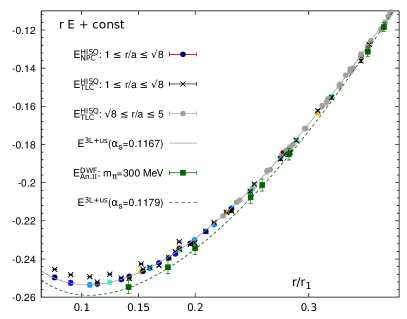
Figure 5: The nonperturbative lattice and the perturbative continuum results for the static energy multiplied by the distance, $rE(r)$ ($E\equiv E_{0}$). The HISQ data Bazavov:2019qoo are nonperturbatively corrected (NPC, colored bullets) or tree-level corrected (TLC, black crosses and gray bullets). The color indicates the lattice spacing in units of the scale $r_{1}$, $\nicefrac{{a}}{{r_{1}}}$. The DWF data Takaura:2018vcy ; Takaura:2018lpw are from a one-step analysis II that mixes the continuum extrapolation with the fit to the OPE result at $\mathrm{N^{3}LO}$, using a parametrization of discretization artifacts (green squares). The lines represent the three-loop result with resummed leading ultrasoft logarithms, corresponding to $\alpha_{S}(m^{2}_{\mathrm{Z}})=0.1167$ (gray, solid) or $\alpha_{S}(m^{2}_{\mathrm{Z}})=0.1179$ (green, dashed). The former uses the central value $\alpha_{S}(m^{2}_{\mathrm{Z}})=0.1167$ of the analysis of the (TLC or NPC) HISQ data with $\nicefrac{{|\bm{r}|}}{{a}}\geq\sqrt{8}$ (gray bullets), the latter uses the central value $\alpha_{S}(m^{2}_{\mathrm{Z}})=0.1179$ of the OPE-based one-step analysis II of the DWF data Takaura:2018vcy ; Takaura:2018lpw . The NPC HISQ data with $\nicefrac{{|\bm{r}|}}{{a}}<\sqrt{8}$ are well-aligned with the fit excluding these data, while the TLC HISQ data with $\nicefrac{{|\bm{r}|}}{{a}}<\sqrt{8}$ cannot be consistently described by a continuum result for any value of $\alpha_{S}(m^{2}_{\mathrm{Z}})$.

For Wilson line correlators, all combinations of $0\leq n_{1},n_{2},n_{3}\leq\nicefrac{{L}}{{2a}}$ are accessible, thus permitting access to non-integer distances in units of the lattice spacing; this entails all of the aforementioned complications. After the nonperturbative correction, $E_{0}^{\mathrm{NPC}}(r_{I},a)$ from Wilson line correlators computed in (2+1)-flavor QCD on lattices with highly improved staggered quarks (HISQ) was shown to exhibit no statistically significant lattice artifacts anymore Bazavov:2019qoo , see Fig. 5. With this data set the range of interest can be probed using a rather large number of $\nicefrac{{r_{I}}}{{a}}$ values and many lattice spacings (up to six spacings in the range $a\in(0.024,\ldots,0.06)\,\mathrm{fm}$), where the underlying high statistics ensembles had been generated for studies of the QCD equation of state HotQCD:2014kol ; Bazavov:2017dsy . The uncertainty due to the lattice scale, lattice spacing dependence, estimates of the uncertainty due to treating residual lattice artifacts with the nonperturbative correction, or due to changes of the fit range are within the the statistical error and subleading in the error budget. Instead it was found that estimates of the continuum perturbative truncation error dominate the error budget. In Ref. Bazavov:2019qoo these have been estimated by a scale variation between $\nicefrac{{2}}{{r}}$ and $\nicefrac{{1}}{{2r}}$, inclusion of a parametric estimate of a higher order term $\pm\nicefrac{{4}}{{3}}\nicefrac{{\alpha_{S}^{5}}}{{r}}$, and variation between resummation or no resummation of the leading ultra-soft logarithms $\nicefrac{{\alpha_{S}^{3+n}\ln^{n}\alpha_{S}}}{{r}}$. The scale dependence becomes non-monotonic below $\nicefrac{{1}}{{\sqrt{2}r}}$ at large $r$, which makes robust error estimates challenging unless the range is restricted to $\max{(|\bm{r}|)}\leq 0.1\,\mathrm{fm}$. As lattice data at larger $|\bm{r}|$ are discarded, the statistical error increases while the truncation error decreases. Eventually, for $\max{(|\bm{r}|)}\ll 0.1\,\mathrm{fm}$, the nonperturbative correction to the lattice data becomes essential to having enough data, while the central value hardly changes. For our joint fit using nonperturbatively corrected HISQ data at five lattice spacings we report the best compromise between the different contributions to the error budget as

$$\alpha_{S}(m^{2}_{\mathrm{Z}})=0.11660^{+0.00110}_{-0.00056},$$ (39)

where the total, symmetric lattice error amounts to $0.00047$ for $|\bm{r}|\leq 0.073\,\mathrm{fm}$.

In Ayala:2020odx , a reanalysis of a subset of these data ($a=0.024\,\mathrm{fm}$, $\sqrt{8}\leq\nicefrac{{|\bm{r}|}}{{a}}\leq 4$) was carried out that included resummation of next-to-leading ultra-soft logarithms $\nicefrac{{\alpha_{S}^{4+n}\ln^{n}{\alpha_{S}}}}{{r}}$, i.e. the full $\mathrm{N^{3}LL}$ accuracy, and hyperasymptotic expansion, resulting in $\alpha_{S}(m^{2}_{\mathrm{Z}})=0.1181(9)$. Concerning the central value, we have already commented that it differs from (39) mostly because of the inclusion of the subleading ultrasoft logarithms. Concerning the error budget, it may possibly increase by including an estimate of the lattice spacing dependence and a variation of $\min{(|\bm{r}|)}$ or $\max{(|\bm{r}|)}$ to smaller values. Nevertheless, even inside the quoted errors the result is consistent with (39).

For Wilson loops, spatial Wilson lines connecting the temporal ones entail additional, $\bm{r}/a$-dependent self-energy divergences. The static energy from Wilson loops is usually computed only for few specific geometries, and spatial link smearing is applied to suppress these divergences. The static energy has been obtained from Wilson loops for two different geometries $\bm{r}/a\propto(1,0,0)$ or $(1,1,0)$ Takaura:2018lpw ; Takaura:2018vcy in (2+1)-flavor QCD on lattices with Möbius domain-wall fermions with a pion mass of $m_{\pi}\approx 300\,\mathrm{MeV}$ and three lattice spacings $a\in(0.04,\ldots,0.08)\,\mathrm{fm}$ that had been generated by the JLQCD collaboration Kaneko:2013jla . Two separate analyses were performed: a two-step analysis (I) with a continuum extrapolation at large distances sequentially followed by the $\alpha_{S}$ extraction, and another one-step analysis (II) using a single joint fit to achieve both at once. Both analyses relied on a particular form of operator product expansion, and used data in the range $0.24\,\mathrm{fm}\leq|\bm{r}|\leq 0.6\,\mathrm{fm}$ or $0.044\,\mathrm{fm}\leq|\bm{r}|\leq 0.36\,\mathrm{fm}$, respectively. The reported values from the two analyses are $\alpha_{S}(m^{2}_{\mathrm{Z}})=0.1166^{+0.0021}_{-0.0020}$ and $\alpha_{S}(m^{2}_{\mathrm{Z}})=0.1179^{+0.0015}_{-0.0014}$. They are both dominated by the estimate of the truncation errors. As both analyses extend far into ranges where $E_{0}(|\bm{r}|,a)$ is known to be sensitive to the pion mass Weber:2018bam , the authors had to include condensate terms, while reporting no significant mass dependence when assuming only a perturbative contribution from massive light quarks. The first analysis has no data for $|\bm{r}|\lesssim 0.10\,\mathrm{fm}$. The second analysis does have data in that region, but has to fit $\Lambda_{\overline{\mathrm{MS}}}$ simultaneously with the lattice artifacts at small $\nicefrac{{\bm{r}}}{{a}}$. As a result the continuum extrapolated static energy from this analysis has large errors for $|\bm{r}|\lesssim 0.10\,\mathrm{fm}$ and lies systematically below the HISQ result from Ref. Bazavov:2019qoo , see Fig. 5.

b Static force

Another possibility consists of computing the force directly from the lattice, i.e.  not as the slope of the static energy. The force, $F$, between a static quark located in ${\bf r}$ and a static antiquark located in ${\bf 0}$ can be defined as Vairo:2015vgb

$$F(r)=\partial_{r}E_{0}(r)=\lim_{T\to\infty}-i\frac{\left\langle\textrm{Tr}\left\{W_{r\times T}\,\hat{\mathbf{r}}\cdot g\mathbf{E}(\mathbf{r},t^{\ast})\right\}\right\rangle}{\langle\textrm{Tr}\{W_{r\times T}\}\rangle}.$$ (40)

The chromoelectric field $\mathbf{E}(\mathbf{r},t^{\ast})$ is located at the quark line of the Wilson loop.

This definition permits to obtain the force directly from the lattice instead of reconstructing it, after interpolation, from the lattice data of the static energy. The perturbative calculation of the force in continuum QCD is free of the leading renormalon and it is known at N³LL. Therefore the force provides a clean way to extract $\alpha_{S}$. In Brambilla:2021wqs , we have used the multilevel algorithm to perform a preliminary quenched lattice study of the chromoelectric insertion in a static Wilson loop given by Eq. (40) both with smeared Wilson loops and with Polyakov loops. The result is consistent with the force obtained via derivative of the static energy upon multiplication with a constant renormalization factor $Z_{E}$ that encodes the very slow convergence of lattice operators containing gluonic operators. Recently in Leino:2021vop we have performed the same calculation with gradient flow, which eliminates the necessity of $Z_{E}$ and makes the lattice calculation more efficient. We plan to go to very fine lattice spacings and perform an extraction of $\Lambda_{\overline{\rm MS}}r_{0}$.

c Static singlet free energy

One reason for which it is challenging to reach the fine lattice spacings needed for the best extraction of $\alpha_{S}$ is that one has to simultaneously maintain the control over finite volume effects from the propagation of the lightest hadronic modes, namely, the pions. A lattice simulation at high enough temperature avoids this infrared problem, and thus enables reaching much finer lattice spacings using smaller volumes. In Bazavov:2019qoo , we considered the extraction of the strong coupling from the singlet free energy at non-zero temperature, as it is expected that at small distances medium effects are small. The singlet free energy in terms of the correlation function of two thermal Wilson lines in Coulomb gauge is given by ($T$ is now the temperature)

$$F_{S}(r,T)=-T\ln\left(\frac{1}{N_{c}}\langle{\rm Tr}\left[W(r)W^{\dagger}(0)\right]\rangle\right).$$ (41)

At distances much smaller than the inverse temperature, $rT\ll 1$, we can write using potential Nonrelativistic QCD Berwein:2017thy

$$F_{S}(r,T)=V_{s}(r,\mu)+\delta F_{S}(r,T,\mu).$$ (42)

The form of the US correction depends on the scale hierarchy which is now featuring also the temperature and the Debye mass $m_{D}\sim gT$: if $1/r\gg\alpha_{S}/r\gg T\gg m_{D}$ then $\mu\sim\alpha_{S}/r$ and $\delta F_{S}(r,T,\mu)=\delta E_{US}(\mu)+\Delta F_{S}(r,T)$, with $\delta E_{US}(\mu)$ being the US contribution to $E_{0}$ in vacuum that we already discussed. The singlet free energy has been studied on the lattice in Ref. Bazavov:2018wmo using a wide temperature range and several lattice spacings, i.e., several temporal extents $N_{\tau}$. The shortest distance that we can access, due to a single lattice spacing on our finest lattice at $T>0$, is $0.00814\,{\rm fm}$. For our analysis the relevant data correspond to $N_{\tau}=10,~{}12$ and $16$, since $rT$ has to be small. From the analysis of Ref. Bazavov:2018wmo we see that thermal effects are small for $rT\lesssim 0.3$. In particular we see that for $|\bm{r}|/a\leq\sqrt{6}$ the difference between the singlet free energy at $(T>0)$ and the static energy at $(T=0)$ approaches a constant proportional to the temperature. No temperature effects beyond a constant can be seen in this range within the errors of the lattice results. Therefore we treat the finite temperature data in this range as if they were at zero temperature and fit them with the three-loop plus leading ultra-soft resummed result of the static energy at $T=0$.

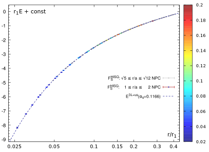
Figure 6: The nonperturbative lattice result $r_{1}E(r)$ ($E\equiv E_{0}$) using the singlet free energy at $T>0$ and the perturbative continuum results for the static energy. The HISQ data Bazavov:2019qoo are nonperturbatively corrected (NPC, colored bullets and gray bullets). The color indicates the lattice spacing in units of the $r_{1}$ scale, $\nicefrac{{a}}{{r_{1}}}$. The dashed line represents the three-loop result with resummed leading ultrasoft logarithms, corresponding to the result of the optimal $T=0$ analysis $\alpha_{S}(m^{2}_{\mathrm{Z}})=0.1166$. Only the NPC HISQ data at $T>0$ with $\nicefrac{{|\bm{r}|}}{{a}}\leq 2$ (colored) are used in the fit, but all data in the range $2<\nicefrac{{|\bm{r}|}}{{a}}\leq\sqrt{12}$ (gray) are still consistent with it.

A drawback of this analysis is the restriction to very small $|\bm{r}|/a$, which implies that the nonperturbative correction (NPC) is indispensable. Yet the main advantage of the analysis is that at very small distances, $\max{(|\bm{r}|)}\leq 0.03\,\mathrm{fm}$, the truncation error becomes very small. Beyond what has been necessary at zero temperature, one must verify that $T>0$ effects do not become significant when including larger $|\bm{r}|/a$ or when varying the temperature $T=\nicefrac{{1}}{{aN_{\tau}}}$ at fixed lattice spacing. We confirmed the statistical irrelevance in these two measures of $T>0$ effects by comparing $\nicefrac{{|\bm{r}|}}{{a}}\leq 2$ with $\nicefrac{{|\bm{r}|}}{{a}}\leq 3$ and $N_{\tau}=12,~{}16$, and, where possible, $64$, and included these error estimates with the other lattice errors in the error budget. The key ingredient to making this extraction work with substantial constraining power is that a wide range in $|\bm{r}|$ can be covered using only narrow windows in $\nicefrac{{|\bm{r}|}}{{a}}$ by performing a joint analysis using multiple lattice spacings $a$ that cover $|\bm{r}|$ in multiple, overlapping segments. For our joint fit using nonperturbatively corrected $T>0$ HISQ data at eight lattice spacings and an $|\bm{r}|$ region and set of lattice spacings non-overlapping with the zero temperature analysis we report

$$\alpha_{S}(m^{2}_{\mathrm{Z}})=0.11638^{+0.00095}_{-0.00087}$$ (43)

(the total, symmetric lattice error amounts to $0.00085$) for $|\bm{r}|\leq 0.03\,\mathrm{fm}$ Bazavov:2019qoo . This result is marginally lower than the result from our zero temperature analysis. Remarkably, however, the zero temperature result is still compatible with the $T>0$ data over a much wider range in $\nicefrac{{|\bm{r}|}}{{a}}$, a factor 16 in $|\bm{r}|$, and over almost a factor 10 in lattice spacings, see Fig. 6.

d Outlook

In summary, in order to reach a few permil accuracy in the extraction of $\alpha_{S}$ with the outlined methods we need:

• Lattice calculations of the static energy at smaller distances, ideally extrapolated to the continuum. The one-loop correction should be computed in lattice perturbation theory. Based on the experience with the nonperturbative correction, the one-loop correction is expected to substantially alleviate the restriction of $\nicefrac{{|\bm{r}|}}{{a}}$ (from $\nicefrac{{|\bm{r}|}}{{a}}\gtrsim 3$ to $\nicefrac{{|\bm{r}|}}{{a}}\gtrsim 2$) in a field-theoretically rigorous manner.

• To exploit more systematically finite temperature simulations in order to go to shorter distances. On the lattice side there is no major impediment to further increasing the temperature and decreasing the lattice spacing.

• To have the non logarithmic four loop contribution to the static potential. This would be important to verify if large numerical cancellations between soft and US contributions also happen beyond three loops.

• To further exploit the definition of the force in terms of a chromoelectric field insertion in the static Wilson loop in order to generate high precision quenched and unquenched lattice data at short distances and to compare with the perturbative expression at N³LO or N³LL.

• To use recent high quality lattice data at 2+1+1 flavors to extract $\alpha_{S}$ from the static energy with an active charm quark Steinbeisser:2021jgc . To achieve precision competitive with 2+1 flavor QCD, a full three-loop calculation of the contribution to the static potential due to the finite charm quark mass may be necessary.

Acknowledgments— P.P. was supported by U.S. Department of Energy under Contract No. DE-SC0012704. J.H.W.’s research was funded by the Deutsche Forschungsgemeinschaft (DFG, German Research Foundation) - Projektnummer 417533893/GRK2575 “Rethinking Quantum Field Theory”.

III $\alpha_{S}(m^{2}_{\mathrm{Z}})$ from hadronic tau decays

1 Determination of $\alpha_{S}(m_{\tau}^{2})$ from ALEPH $\tau$ decay data

The inclusive distribution of the final hadrons in $\tau$ decay provides the needed information to perform a clean low-energy determination of the strong coupling Pich:2020gzz . The relevant dynamical quantities are the two-point correlation functions for the vector $V^{\mu}=\overline{u}\gamma^{\mu}d$ and axial-vector $A^{\mu}=\overline{u}\gamma^{\mu}\gamma_{5}d$ colour-singlet charged currents:

$$i\int d^{4}x\;e^{iqx}\;\bra{0}T[\mathcal{J}^{\mu}(x)\mathcal{J}^{\nu\dagger}(0)]\ket{0}\,=\,(-g^{\mu\nu}q^{2}+q^{\mu}q^{\nu})\;\Pi_{\mathcal{J}}(q^{2})+g^{\mu\nu}q^{2}\;\Pi^{(0)}_{\mathcal{J}}(q^{2})\,,$$ (44)

with $\mathcal{J}=V,A$. If the tiny up and down quark masses are neglected, $q^{2}\;\Pi^{(0)}_{\mathcal{J}}(q^{2})=0$ and only the first term needs to be considered. The correlators $\Pi_{\mathcal{J}}(s)$ are analytic functions in the entire complex $s$ plane, except for a cut along the positive real axis where their imaginary parts (spectral functions) have discontinuities. This implies the exact mathematical identity Braaten:1991qm

$$A^{\omega}_{\mathcal{J}}(s_{0})\;\equiv\;\int^{s_{0}}_{s_{\mathrm{th}}}\frac{ds}{s_{0}}\;\omega(s)\,\mathrm{Im}\Pi_{\mathcal{J}}(s)\;=\;\frac{i}{2}\;\oint_{|s|=s_{0}}\frac{ds}{s_{0}}\;\omega(s)\,\Pi_{\mathcal{J}}(s)\,,$$ (45)

where $\omega(s)$ is any weight function analytic in $|s|\leq s_{0}$, $s_{\mathrm{th}}$ is the hadronic mass-squared threshold, and the complex integral in the right-hand side runs counter-clockwise around the circle $|s|=s_{0}$. The inclusive Cabibbo-allowed hadronic decay width of the $\tau$ just corresponds to the weight $\omega_{\tau}(x)=(1-x)^{2}(1+2x)$ with $x=s/s_{0}$ and $s_{0}=m_{\tau}^{2}$. The measured invariant-mass distribution determines then the left-hand-side integral for $s_{0}\leq m_{\tau}^{2}$.

For large-enough values of $s_{0}$, the operator product expansion (OPE) Shifman:1978bx ,

$$\Pi^{\mathrm{OPE}}_{\mathcal{J}}(s)\;=\;\sum_{D}\frac{1}{(-s)^{D/2}}\sum_{\mathrm{dim}\,\mathcal{O}=D}C_{D,\mathcal{J}}(-s,\mu)\;\langle 0|\mathcal{O}(\mu)|0\rangle\;\equiv\;\sum_{D}\;\dfrac{\mathcal{O}_{D,\,\mathcal{J}}}{(-s)^{D/2}}\,,$$ (46)

can be used to expand the contour integral in inverse powers of $s_{0}$. The first term ($D=0$) contains the perturbative QCD contribution, which is known to $\mathcal{O}(\alpha_{S}^{4})$ Baikov:2008jh , while nonperturbative power corrections have $D\geq 4$. The small differences between the physical values of the integrated moments $A^{\omega}_{\mathcal{J}}(s_{0})$ and their OPE approximations are known as quark-hadron duality violations. They are very efficiently minimized by taking “pinched” weight functions which vanish at $s=s_{0}$, suppressing in this way the contributions from the region near the real axis where the OPE is not valid Braaten:1991qm ; LeDiberder:1992zhd ; Gonzalez-Alonso:2016ndl .

The high sensitivity of the $\tau$ hadronic width to the strong coupling follows from four important facts:

1. The perturbative contribution amounts to a sizeable 20% effect because $\alpha_{S}(m_{\tau}^{2})\sim 0.3$ is large.

2. The OPE can be safely used at $s_{0}\sim m_{\tau}^{2}$. The weight $\omega_{\tau}(x)$ contains a double zero at $s=s_{0}$, heavily suppressing the numerical impact of duality violations.

3. Since $\omega_{\tau}(x)=1-3x^{2}+2x^{3}$, the contour integral is only sensitive to OPE corrections with $D=6$ and 8, which are strongly suppressed by the corresponding powers of $m_{\tau}$. Moreover, these power corrections appear with opposite signs in the vector and axial-vector correlators Braaten:1991qm ; Davier:2013sfa ; Pich:2016bdg , which implies an additional numerical cancellation in the total vector $+$ axial ($V+A$) decay width.

4. The opening of high-multiplicity hadronic thresholds dilutes very soon the prominent $\rho(2\pi)$ and $a_{1}(3\pi)$ resonances, leading to a quite flat $V+A$ spectral distribution that approaches very fast the perturbative QCD predictions.

The small nonperturbative contributions can be extracted from data, analysing moments more sensitive to power corrections LeDiberder:1992zhd . The detailed analyses performed by ALEPH ALEPH:2005qgp , CLEO CLEO:1995nlc and OPAL OPAL:1998rrm confirmed a long time ago that these corrections are smaller than the perturbative uncertainties. The latest and more precise experimental determination of the strong coupling obtains $\alpha_{S}^{(n_{f}=3)}(m_{\tau}^{2})=0.332\pm 0.005_{\mathrm{exp}}\pm 0.011_{\mathrm{th}}$ Davier:2013sfa . Taking as input their measured nonperturbative correction, the strong coupling can be directly extracted from the total $\tau$ hadronic width (and/or lifetime), which results in $\alpha_{S}^{(n_{f}=3)}(m_{\tau}^{2})=0.331\pm 0.013$ Pich:2013lsa .

An exhaustive reanalysis with the updated ALEPH $\tau$ data Davier:2013sfa has been performed in Ref. Pich:2016bdg , in order to carefully assess any possible source of systematic uncertainties. A large variety of methodologies, including all previously considered strategies, have been explored, looking for potential hidden weaknesses and testing the stability of the fitted results under slight variations of the assumed inputs. The most reliable determinations of $\alpha_{S}(m_{\tau}^{2})$, obtained with the total $V+A$ distribution, are summarized in Table 4. The dominant uncertainties are the perturbative errors associated with the unknown higher-order corrections. This is clearly illustrated in the table, which shows the results obtained under two different procedures, either performing the contour integrals with a running $\alpha_{S}(-s)$, by solving numerically the five-loop $\beta$-function equation (contour-improved perturbation theory, CIPT) LeDiberder:1992jjr ; Pivovarov:1991rh , or naively expanding them in powers of $\alpha_{S}(m_{\tau}^{2})$ (fixed-order perturbation theory, FOPT). FOPT generates a somewhat larger perturbative contribution and, therefore, leads to a slightly smaller fitted value of $\alpha_{S}$. Within each procedure, the perturbative error has been estimated taking a very conservative range for the fifth-order coefficient of the Adler series, $K_{5}=275\pm 400$, and varying the renormalization scale in the interval $\mu^{2}/(-s)\in(0.5,2)$. The values obtained with the two procedures are finally combined, adding quadratically half their difference as an additional systematic error.

Table 4: Determinations of $\alpha_{S}^{(n_{f}=3)}(m_{\tau}^{2})$ from $\tau$ decay data, in the $V+A$ channel Pich:2016bdg .

Method
	$\alpha_{S}^{(n_{f}=3)}(m_{\tau}^{2})$
	CIPT	FOPT	Average
$\omega_{kl}(x)$ weights	$0.339\,{}^{+\,0.019}_{-\,0.017}$	$0.319\,{}^{+\,0.017}_{-\,0.015}$	$0.329\,{}^{+\,0.020}_{-\,0.018}$
$\hat{\omega}_{kl}(x)$ weights	$0.338\,{}^{+\,0.014}_{-\,0.012}$	$0.319\,{}^{+\,0.013}_{-\,0.010}$	$0.329\,{}^{+\,0.016}_{-\,0.014}$
$\omega^{(2,m)}(x)$ weights	$0.336\,{}^{+\,0.018}_{-\,0.016}$	$0.317\,{}^{+\,0.015}_{-\,0.013}$	$0.326\,{}^{+\,0.018}_{-\,0.016}$
$s_{0}$ dependence	$0.335\pm 0.014$	$0.323\pm 0.012$	$0.329\pm 0.013$
$\omega_{a}^{(1,m)}(x)$ weights	$0.328\,{}^{+\,0.014}_{-\,0.013}$	$0.318\,{}^{+\,0.015}_{-\,0.012}$	$0.323\,{}^{+\,0.015}_{-\,0.013}$
Average	$0.335\pm 0.013$	$0.320\pm 0.012$	$0.328\pm 0.013$

The different rows in the table correspond to different choices of pinched weights:

$$\omega_{kl}(x) =(1-x)^{2+k}\,x^{l}\,(1+2x)\,,\qquad\qquad (k,l)=\{(0,0),\, (1,0),(1,1),(1,2),(1,3)\}\,,$$

$$\hat{\omega}_{kl}(x) =(1-x)^{2+k}\,x^{l}\,,\qquad\qquad (k,l)=\{(0,0),\, (1,0),(1,1),(1,2),(1,3)\}\,,$$

$$\omega^{(2,m)}(x) =1-(m+2)\,x^{m+1}+(m+1)\,x^{m+2}\,, 1\leq m\leq 5\,,$$

$$\omega_{a}^{(1,m)}(x) =(1-x^{m+1})\,\mathrm{e}^{-ax}\,, 0\leq m\leq 6\,.$$ (47)

In all cases, we find a high sensitivity to the strong coupling and a very small sensitivity to power corrections, which gets reflected in large uncertainties for the fitted condensates. The first set of weights was adopted by ALEPH and allows for a direct use of the measured distribution. With the five indicated moments, we have fitted $\alpha_{S}(m_{\tau}^{2})$ and the nonperturbative corrections $\mathcal{O}_{4,6,8}$. The impact on $\alpha_{S}$ from neglected condensates of higher dimensions (the highest moment involves corrections with $D\leq 16$) has been estimated including $\mathcal{O}_{10}$ in the fit and taking the difference as an additional uncertainty. Additional power corrections with $D>10$ would certainly modify the poorly determined values of the fitted condensates, specially those with higher dimensions, but they have a negligible impact on $\alpha_{S}$, compared with the errors already included. Our results (first line in the table) are in good agreement with Ref. Davier:2013sfa . Very similar values are obtained with the modified weights $\hat{\omega}_{kl}(x)$ (second line), which eliminate the highest-$D$ power correction from every moment, showing that these contributions do indeed play a minor numerical role.

Moments constructed with the optimized (double-pinched) weights $\omega^{(2,m)}(x)$ only receive power corrections with $D=2(m+2)$ and $2(m+3)$. The third line in the table shows that they give values of $\alpha_{S}(m_{\tau}^{2})$ in very good agreement with those in the first two lines. Similar results (not shown in the table) are obtained from a fit to four moments, based on the weights $\omega^{(n,0)}(x)=(1-x)^{n}$, with $0\leq n\leq 3$, which have a different sensitivity to power corrections and (for $n=0,1$) are less protected against duality violations and experimental uncertainties. The values of $\alpha_{S}(m_{\tau}^{2})$, $\mathcal{O}_{2(m+2)}$ and $\mathcal{O}_{2(m+3)}$ can also be extracted from a fit to the $s_{0}$ dependence of a single $A^{(2,m)}(s_{0})$ moment, above some $\hat{s}_{0}\geq 2.0\;\mathrm{GeV}^{2}$. One finds a quite poor sensitivity to power corrections, as expected, but a surprising stability in the extracted values of $\alpha_{S}(m_{\tau}^{2})$ at different $\hat{s}_{0}$. Combining the information from three different moments ($m=0,1,2$), and adding as an additional theoretical error the fluctuations with the number of fitted bins, one gets the $\alpha_{S}(m_{\tau}^{2})$ values given in the fourth line of Table 4. This determination is much more sensitive to violations of quark-hadron duality because the $s_{0}$ dependence of consecutive bins feels the local structure of the spectral function. The agreement with the determinations in the other lines of the table confirms the small size of duality violations in the $V+A$ distribution above $\hat{s}_{0}$.

A completely different sensitivity to nonperturbative corrections is achieved with the weights $\omega_{a}^{(1,m)}$. Their exponential suppression nullifies the high-$s$ region, strongly reducing the violations of quark-hadron duality, at the price of enhancing the exposition to power corrections of any dimensionality. In a pure perturbative analysis the neglected power corrections should manifest as large instabilities of $\alpha_{S}$ under variations of $s_{0}$ and $a\not=0$; however, stable results are found for a broad range of both $s_{0}$ and $a$, which indicates that power corrections are small. The last line in the table has been obtained combining the information from seven different moments with $\omega_{a}^{(1,m)}$ ($0\leq m\leq 6$) weights.

Fully compatible results with slightly larger uncertainties are also obtained from the separate $V$ and $A$ distributions Pich:2016bdg . The excellent overall agreement among determinations obtained with a broad variety of numerical approaches that have very different sensitivities to nonperturbative corrections, and the many complementary tests successfully performed in Ref. Pich:2016bdg , demonstrate the robustness and reliability of the results shown in Table 4. The final average value

$$\alpha_{S}^{(n_{f}=3)}(m_{\tau}^{2})\,=\,0.328\pm 0.013$$ (48)

is in good agreement with the results of Ref. Davier:2013sfa and with a recent determination (see Sect. 3) based on Borel–Laplace sum rules and a renormalon-motivated model Ayala:2021yct . After evolution up to the scale $m_{\mathrm{Z}}$, the strong coupling decreases to

$$\alpha_{S}^{(n_{f}=5)}(m_{\mathrm{Z}}^{2})\,=\,0.1197\pm 0.0015\,,$$ (49)

in excellent agreement with the direct N³LO determination at the Z peak.

A much better control of the small nonperturbative contributions could be achieved with more precise data, specially at the highest energy bins. The high-statistics expected from Belle-II or a future TeraZ facility should make that possible. A reduction of the dominant perturbative error requires a better theoretical understanding of higher-order corrections (CIPT versus FOPT, renormalons, etc.). In the long term, an explicit calculation of the $K_{5}$ term in the Adler series would have a major impact.

Acknowledgments— This work has been supported by MCIN/AEI/10.13039/501100011033, Grant No. PID2020-114473GB-I00, by the Generalitat Valenciana, Grant No. Prometeo/2021/071, and by the Agence Nationale de la Recherche (ANR), Grant ANR-19-CE31-0012 (project MORA).

2 The strong coupling from hadronic $\tau$ decays: present and future

We review the sum-rule framework for determining the strong coupling, $\alpha_{S}$, from inclusive spectral functions measured in hadronic $\tau$ decays. We then discuss a new inclusive vector isovector spectral function, obtained from combining the dominant exclusive-mode spectral-function data from ALEPH and OPAL with BaBar data for $\tau\to K^{-}K^{0}\nu_{\tau}$ and several CVC-converted $R$-ratio data sets for small exclusive-mode contributions that had previously been estimated using Monte Carlo methods. We summarize our most recent results for $\alpha_{S}$, and discuss prospects for future improvements.

a Review

Finite-energy sum rules (FESRs) allow for the extraction of the strong coupling at the $\tau$ mass, $\alpha_{S}(m_{\tau}^{2})$, from inclusive vector ($V$) and/or axial ($A$) non-strange spectral functions, which can and have been measured through hadronic $\tau$ decays OPAL:1998rrm ; ALEPH:1998rgl ; ALEPH:2005qgp . Such sum rules have the form

$$I^{(w)}(s_{0})\equiv\frac{1}{s_{0}}\int_{0}^{s_{0}}ds\,w(s)\,\rho(s)=-\frac{1}{2\pi is_{0}}\oint_{|z|=s_{0}}dz\,w(z)\,\Pi(z)\ ,$$ (50)

where $\Pi(z)$ is a vacuum polarization, $\rho(s)=\frac{1}{\pi}\mbox{Im}\,\Pi(s)$, with $s=q^{2}$, is the corresponding spectral function, $s_{0}>0$, and $w(s)$ is typically a polynomial in $s/s_{0}$. The left-hand side of Eq. (50) can be determined from data for $s_{0}\leq m_{\tau}^{2}$, while, for $s_{0}$ large enough, the right-hand side can be represented in QCD perturbation theory, with nonperturbative (NP) corrections. The latter are needed because of the relatively low value of $m_{\tau}$.

The perturbative expansion for $\Pi(z)$ in powers of $\alpha_{S}(\mu^{2})$ and $\log(-z/\mu^{2})$ is known to order $\alpha_{S}^{4}$ Baikov:2008jh , where $\mu$ is the renormalization-group scale. In most of the literature, two scale-choice prescriptions have been considered, either FOPT, in which $\mu^{2}=s_{0}$, or CIPT Pivovarov:1991rh ; LeDiberder:1992jjr , in which $\mu^{2}$ is set equal to $z$ when evaluating the perturbative contribution to the contour integral on the right-hand side of Eq. (50).

NP corrections (away from the positive real axis, see below) are incorporated through the operator product expansion (OPE), which schematically takes the form

$$\Pi_{\mathrm{OPE}}(z)=\sum_{k=0}^{\infty}(-1)^{k}\frac{C_{2k}(z)}{z^{k}}\ .$$ (51)

The $k=0$ term represents purely perturbative contributions, the $k=1$ term perturbative mass corrections (in the non-strange channels, $C_{2}$ can be set to zero because of the smallness of the up and down quark masses); NP condensate contributions start at $k=2$. The presence of a cut in the complex $z=q^{2}$ plane extending to infinity along the positive real axis, means the OPE is not convergent; it is, at best, an asymptotic series. It is also generally believed that the $D=2k$ terms (for $k>1$) are related to renormalon ambiguities in the perturbative expansion Beneke:1998ui ; Beneke:2008ad ; Beneke:2012vb . While the higher-dimension coefficients $C_{2k}$ in principle depend logarithmically on $z$, they are generally taken as constants, as their $z$ dependence is suppressed by two powers of $\alpha_{S}$, in addition to the $1/z^{k}$ suppression.

Recently, it was shown that the Borel sums of the FOPT and CIPT versions of the perturbative expansion of the right-hand side of Eq. (50) are not the same, and, related, that the OPE (51) does not reflect the renormalon ambiguities for CIPT Hoang:2020mkw ; Hoang:2021nlz , creating a mismatch between the use of CIPT and the OPE in the form (51). Because of this, we will always employ FOPT Boito:2020xli . The recent work of Ref. Benitez-Rathgeb:2022yqb (see Sec. 4) paves the way for a reconciliation between the FOPT and CIPT series but, until this is realized in practice, averaging the results obtained using FOPT and CIPT should be avoided.

The nonconvergent, at-best-asymptotic, nature of the OPE noted above has two implications. First, it is advisable to restrict the use of the OPE to low orders in the expansion (51), as little is known about where it starts to diverge (at the energies relevant in $\tau$ decays). Second, one expects NP corrections beyond the OPE, just as the OPE represents NP corrections beyond perturbation theory. This phenomenon, known as the violation of quark-hadron duality Poggio:1975af ; Blok:1997hs ; Bigi:1998kc , manifests itself physically in the presence of overlapping resonance contributions in $\rho(s)$. These duality violations (DVs) need to be modeled (as long as a NP solution to QCD is not known). We have developed a theoretical framework, based on generally accepted assumptions about QCD in the framework of hyperasymptotics Boito:2017cnp , which leads to the following large-$s$ asympotic form for the duality-violating part of the spectral function:

$$\rho_{\mathrm{DV}}(s)=e^{-\delta-\gamma s}\sin\left(\alpha+\beta s\right)\left[1+{\cal{O}}\left(\frac{1}{\log{s}};\,\frac{1}{s};\,\frac{1}{N_{c}}\right)\right]\ .$$ (52)

With this ansatz, the sum rule (50) can be reformulated as Cata:2005zj

$$\frac{1}{s_{0}}\int_{0}^{s_{0}}ds\,w(s)\,\rho(s)=-\frac{1}{2\pi is_{0}}\oint_{|z|=s_{0}}dz\,w(z)\,\Pi_{\mathrm{OPE}}(z)-\frac{1}{s_{0}}\int_{s_{0}}^{\infty}ds\,w(s)\,\rho_{\mathrm{DV}}(s)\ .$$ (53)

This introduces a new set of parameters into the theory representation of the right-hand side of Eq. (50). A separate set of DV parameters is needed for each of the $V$ and $A$ channels. The main assumption is that the form (52) can be used at values of $s$ below $m_{\tau}^{2}$—whether this is the case can be tested by a variety of fits to data. For a more detailed version of this very brief review, and many more references, we refer to Ref. Boito:2020xli .

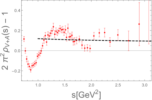
Figure 7: Blow-up of the large-$s$ region of the parton-model-subtracted ALEPH $V+A$ non-strange spectral function Davier:2013sfa . The dashed curve represents QCD perturbation theory.

At this point, a quick look at data is instructive. Figure 7 shows a rescaled version of the sum of the non-strange $V$ and $A$ spectral functions from Ref. Davier:2013sfa , with the $\alpha_{S}$-independent parton-model contribution subtracted. Resonance oscillations are immediately evident, with an amplitude comparable in size to the $\alpha_{S}$-dependent pQCD contribution, represented by the dashed curve. The figure makes clear that DVs are important, though, because of the large errors, it is difficult to tell whether oscillations above $s=m_{\tau}^{2}$ (relevant to determining DV contributions to the sum rules (53) with $s_{0}=m_{\tau}^{2}$) will be numerically relevant or not. Clearly, DVs need to be accounted for, and their contributions quantitatively assessed, even in the $V+A$ channel.

Two different strategies, which we refer to as the “truncated OPE” (tOPE) LeDiberder:1992zhd and the “DV-model” strategies Boito:2011qt ; Boito:2012cr , have been developed to deal with the NP contributions discussed above.

In the tOPE approach, $s_{0}$ is taken equal to $m_{\tau}^{2}$, and, to suppress contributions to the contour integral from the region near the positive real axis, and thus from DVs, weights with a double or triple zero at $s=s_{0}=m_{\tau}^{2}$ are employed. The set of such multiple-zero (“pinched”) polynomial weights typically extends up to degree $k=7$, and thus probes the OPE up to dimension $D=2k+2=16$. The number of OPE parameters to be fitted ($\alpha_{S}$ and the condensates $C_{D}$, $D=4,\,6,\cdots,\,16$) necessarily exceeds the number of such independent weights, and hence the number of independent $s_{0}=m_{\tau}^{2}$ spectral integrals available to fix these parameters. Some subset of the $C_{D}$ in principle present must thus be set to zero by hand to leave a fit with fewer parameters than data points. DVs are also neglected (in terms of Eq. (52), $\delta$ is set to $\infty$) under the assumption that the use of pinched moments sufficiently suppressess these contributions.

The main problem with this strategy, employed most recently in Refs. Davier:2013sfa ; Pich:2016bdg , is the neglect of these higher-$D$ OPE contributions. Several tests of the tOPE strategy were carried out in Refs. Boito:2016oam ; Boito:2019iwh , exposing clear inconsistencies. Such inconsistencies can arise because integrated dimension-$D$ OPE contributions scale as $1/s_{0}^{D/2}$. If contributions from omitted higher-$D$ condensates are, in fact, not numerically negligible, then when these are absorbed into the values of the lower-$D$ OPE parameters obtained in a fixed-$s_{0}$ tOPE fit, the resulting theory representation will, in general, have an $s_{0}$ dependence which is incorrect. The tOPE truncation can thus be tested for self-consistency by comparing spectral-integral predictions obtained using the theory parameters obtained from the single-$s_{0}$ tOPE fit to the experimental values of these same spectral integrals over a range of $s_{0}$ values. Such tests, designed to take into account the impact of the very strong correlations between (i) spectral integrals at different $s_{0}$, (ii) theory integrals at different $s_{0}$, and (iii) fitted theory parameters and spectral integrals, were carried out in Ref. Boito:2019iwh , with related tests also carried out in Ref. Boito:2016oam . The $s_{0}$ dependence of the theory predictions was found to be in clear disagreement with that of the corresponding experimental spectral integral combinations.

To date, the proponents of the tOPE have yet to provide a peer-reviewed-journal response addressing the inconsistencies of the tOPE approach identified in Refs. Boito:2016oam ; Boito:2019iwh . Such a response is required to make progress on resolving the ongoing controversy over the reliability of the tOPE strategy. Contributions to conference proceedings, though useful, typically do not allow for the level of detailed discussion necessary to produce a resolution of this type of controversy.

In the alternate DV-model strategy, recent implementations employ weights sensitive to terms in the OPE only up to $D=8$, avoiding potential problems with higher-$D$ OPE contributions. DVs cannot, in general, be ignored, and are instead modeled by Eq. (52), with fits performed to spectral integrals for a range of $s_{0}$ between a minimum value $s_{0}^{min}$ and $m_{\tau}^{2}$, where $s_{0}^{min}$ is determined by the quality of the fits and turns out to be $\sim 1.5$ GeV². Results are found to be very stable against variations of $s_{0}^{min}$.

To determine both DV parameters and $\alpha_{S}$, the analysis should include at least one weight with good sensitivity to DVs. The choice $w=1$, which produces no DV suppression, is ideal for this purpose. Stability of the DV-model approach has been tested using various combinations of weight functions in analyses of purely $V$-channel $\tau$ data, both $V$- and $A$-channel $\tau$ data Boito:2014sta , and the KNT Keshavarzi:2018mgv ; Keshavarzi:2019abf compilation of $R$-ratio (inclusive $e^{+}e^{-}\to\mbox{hadrons}$) data Boito:2018yvl . Ref. Boito:2020xli contains our most recent application of this strategy. Earlier applications, laying out the framework in more detail, can be found in Ref. Boito:2011qt . The DV-model strategy uses a range of $s_{0}$ as it is important to check the $s_{0}$ dependence of the match between experiment and theory (left-hand and right-hand sides of Eq. (53), respectively), to test the validity of the theory representation employed for $\Pi(z)$. One also needs to check that oscillations in the $V$ and $A$ (hence also $V+A$) spectral functions are well represented by the ansatz (52), for at least some range of $s$ below $m_{\tau}^{2}$.

As is often the case at conferences and workshops, the time available for the tau discussion session at this workshop turned out to be too short to address, in sufficient detail, a number of ongoing misconceptions and/or mis-statements concerning the tOPE and DV model approaches. In this regard, a useful tool provided by the workshop organizers was the associated CERN mattermost channel, mattermost.web.cern.ch/alphas-2022/channels/town-square, where, in M. Golterman’s February 14 posting, an expanded discussion dealing with and correcting a number of these mis-statements/misconceptions can be found.

b Data

Traditionally, in most papers since the appearance of the perturbative result to order $\alpha_{S}^{4}$ in Ref. Baikov:2008jh , the $\tau$-based $\alpha_{S}$ has been obtained from the ALEPH data Davier:2013sfa ; Pich:2016bdg ; Boito:2014sta ; Ayala:2021mwc ; Ayala:2021yct . However, the value obtained from OPAL data Boito:2011qt ; Boito:2012cr is consistent with the ALEPH-based result Boito:2014sta , and it thus makes sense to combine the ALEPH and OPAL data sets prior to integration, following the approach now routinely employed for electroproduction data when obtaining dispersive estimates for the leading hadronic contribution to the muon anomalous magnetic moment. Moreover, while the bulk of the inclusive spectral functions comes from the 2-pion and the 4-pion modes (in the $V$ channel), and the 3-pion and 5-pion modes (in the $A$ channel), most of the residual exclusive channels (including some of the 5-pion channels) were obtained from Monte-Carlo rather than from experimental data in Refs. OPAL:1998rrm ; ALEPH:1998rgl ; ALEPH:2005qgp . In the $V$ channel, this can now be remedied by using, in addition to BaBar results for $\tau\to K^{-}K^{0}\nu_{\tau}$ BaBar:2018qry , recent high-precision results for higher-multiplicity, $G$-parity positive (hence $I=1$) exclusive-mode electroproduction cross sections. CVC allows these to be converted to the equivalent higher-multiplicity contributions to the $I=1$, $V$ $\tau$-based spectral function. The detailed construction of the combined inclusive $I=1$, $V$ spectral function along these lines is described in Ref. Boito:2020xli . With 98% of the inclusive total by branching fraction (BF) coming from the combined ALEPH and OPAL 2-pion and 4-pion modes, and the support for the residual modes lying well above the $\rho/\omega$ interference region, isospin-breaking corrections, which should in principle be applied to the CVC relations, will be safely negligible.

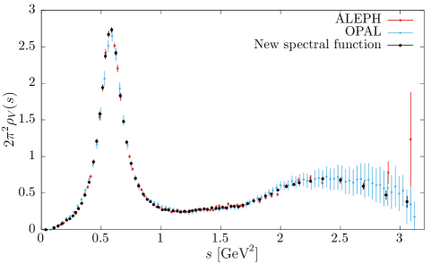
Figure 8: New non-strange $V$ spectral function Boito:2020xli , compared with the ALEPH and OPAL spectralfunctions.

The new $V$ spectral function is shown in Fig. 8. The increased precision in the large-$s$ region, coming from the replacement of Monte-Carlo data with electroproduction data (which are not kinematically limited by the $\tau$ mass) is immediately evident. A more quantitative measure of the improved precision is provided in Table 5, which shows a dramatically reduced statistical error on the $w=1$ spectral moment $I^{(w=1)}(s_{0})$ resulting from the improved precision of the combined spectral function, compared to the ALEPH or OPAL spectral functions, in the larger $s$ region.

Table 5: Comparison of the left-hand side of Eq. (50) for $w=1$, at two values of $s_{0}$, for the combined, ALEPH, and OPAL versions of the $V$ spectral function. $s_{0}^{*}$ is a value close to $1.5$ GeV² for each case, and $s_{0}^{**}$ is close to $2.9$ GeV² for each case. Note that, because the values of $s_{0}^{*}$ and $s_{0}^{**}$ are slightly different for the three cases, the central values cannot be directly compared. The errors can, however, be compared, as they vary slowly with $s_{0}$. For details, see Ref. Boito:2020xli .

	combined	ALEPH	OPAL
$s_{0}^{*}\approx 1.5$ GeV2	0.03137(14)	0.03145(17)	0.03140(46)
$s_{0}^{**}\approx 2.9$ GeV2	0.02952(29)	0.03133(65)	0.03030(170)

c Results

The increased precision of the new non-strange $I=1$ $V$ spectral function constructed in Ref. Boito:2020xli produces an improved determination of $\alpha_{S}(m_{\tau}^{2})$, with the CVC-based improvement of residual-mode contributions playing a particularly important role. Since electroproduction data are purely vector, a similar improvement is not possible for the axial channel. Higher precision is thus now obtainable from $V$-channel than from $V+A$-channel analyses.

Our result for $\alpha_{S}$ at the $\tau$-mass is Boito:2020xli

$$\alpha_{S}(m_{\tau}^{2})=0.3077\pm 0.0065_{\mathrm{exp}}\pm 0.0038_{\mathrm{theory}}\\ =0.3077\pm 0.0075\qquad(n_{f}=3\ ,\ \mbox{FOPT})\ ,$$ (54)

where the first error is the fit error, and the second an estimate of the systematic uncertainty associated with the truncation of perturbation theory and the use of Eq. (52) to model DVs. For comparison, analyses of ALEPH or OPAL data alone produce combined errors of $\pm 0.010$ and $\pm 0.018$, respectively.

Converting Eq. (54) to the $n_{f}=5$, Z-mass scale using five-loop running and four-loop matching at the charm and bottom thresholds, one finds

$$\alpha_{S}(m^{2}_{\mathrm{Z}})=0.1171\pm 0.0010\qquad(\tau\ ,\ n_{f}=5\ ,\ \mbox{FOPT})\ .$$ (55)

This is in good agreement with an independent determination from electroproduction data using the same theoretical framework Boito:2018yvl :

$$\alpha_{S}(m^{2}_{\mathrm{Z}})=0.1158\pm 0.0022\qquad(\mbox{EM}\ ,\ n_{f}=5\ ,\ \mbox{FOPT})\ .$$ (56)

The latter determination was obtained from FESRs with $3.25$ GeV${}^{2}\leq s_{0}^{min}\leq 4$ GeV², significantly higher than the interval $\sim 1.5$ GeV${}^{2}\leq s_{0}^{min}\leq m_{\tau}^{2}$ available from $\tau$ decays. The wider range of accessible $s_{0}$ allowed tests of our model for DVs, Eq. (52), to be performed by comparing values of $\alpha_{S}(m_{\tau}^{2})$ obtained from the $w=1$ FESR (which is maximally sensitive to DV effects, and hence provides a good probe of their effect) with and without DV contributions included. The effect found was small (of order $0.005$) for $3.25$ GeV${}^{2}\leq s_{0}^{min}\leq 4$ GeV² but increased rapidly as $s_{0}^{min}$ was lowered below $m_{\tau}^{2}$.

d Future improvements

The value of $\alpha_{S}$ obtained from hadronic $\tau$ decays, in addition to being competitive, provides a particularly strong test of the running predicted by QCD since the $\tau$ mass is much lower than the energies at which other determinations have been carried out. Important questions are, of course, what future data or theory improvements might produce a reduction in the error on the current best result, Eq. (54), and how to test the assumed NP behavior of the spectral function around and below the $\tau$ mass. As we will now discuss, the best prospect for improvement appears to be from future, more precise data for hadronic $\tau$ decays.

Improved $\tau$ data will allow for a reduction in the experimental part of the error on $\alpha_{S}(m_{\tau}^{2})$, currently $\pm 0.0065$. The theory error in Eq. (54) has two (to some extent related) sources: the truncation of perturbation theory, and the unavoidable need to estimate NP effects. A calculation of the order-$\alpha_{S}^{5}$ term in QCD perturbation theory would be interesting, given the sometimes slow convergence of $I^{(w)}(s_{0})$ for typical weights $w$. On the nonperturbative side, increased data precision would allow more stringent tests, in particular of the DV contribution from Eq. (52). Subleading effects predicted by Ref. Boito:2017cnp might become accessible, and either further confirmation, or a breakdown of this representation of DVs would increase our ability to probe the limits on the potential precision of the strong-coupling determination from hadronic $\tau$ decays.

A further point, of relevance to improving tests of the reliability of the theoretical assumptions underlying the two FESR approaches, concerns how such tests should be carried out. In the past, overlapping experimental spectral integral and theory integral error bands were often taken as evidence of the compatibility of the underlying theory representation with data. Such a conclusion is, however, statistically unjustified since the theory errors, which result from a fit to the experimental spectral integrals, are necessarily very strongly correlated with their experimental counterparts. Plotting both, and interpreting their overlap as if the two were independent runs the risk of serious double counting. To properly test underlying theory assumptions, it is crucial to make comparisons that account for not just correlations between the spectral integrals at different $s_{0}$ and theory integrals at different $s_{0}$, but also those between fitted theory and experimental integrals.

While FCC-ee would produce $\tau$-leptons copiously FCC:2018evy ; Dam:2021ibi , the best near-future prospect is Belle-II Belle:2008xpe , which has access to many more $\tau$-leptons than were produced at LEP. Our construction of the new inclusive $V$ spectral function, moreover, suggests a clear path forward: no fully-inclusive spectral function needs to be obtained from Belle-II data. Residual-mode contributions (which, though representing only 2% of the inclusive total by BF, are important in the upper part of the $\tau$ kinematic range) have already been brought under good control using CVC and electroproduction data Boito:2020xli . More precise 2-pion and 4-pion exclusive-mode $\tau$ data would thus suffice to produce a new $I=1$ $V$ spectral function with even smaller errors than those of Ref. Boito:2020xli , and hence to reduce the experimental error in Eq. (54). Details will need to be carefully considered. For instance, while the existing Belle unit-normalized 2-pion distribution is more precise than that of ALEPH or OPAL, the $\tau\to\pi^{-}\pi^{0}\nu_{\tau}$ BF has been measured less well by Belle, with the HFLAV HFLAV:2019otj value still dominated by ALEPH. An improved, BF-normalized 2-pion distribution will thus require combining input from different experiments. The situation is, presumably, similar for the two 4-pion modes.

Acknowledgments— DB is supported by the São Paulo Research Foundation (FAPESP) Grant No. 2021/06756-6, by CNPq Grant No. 309847/2018-4, and by the Coordenação de Aperfeiçoamento de Pessoal de Nível Superior—Brazil (CAPES)—Finance Code 001. MG is supported by the U.S. Department of Energy, Office of Science, Office of High Energy Physics, under Award No. DE-SC0013682. KM is supported by a grant from the Natural Sciences and Engineering Research Council of Canada. SP is supported by the Spanish Ministry of Science, Innovation and Universities (project PID2020-112965GB-I00/AEI/10.13039/501100011033). IFAE is partially funded by the CERCA program of the Generalitat de Catalunya.

3 Extraction of $\alpha_{S}$ using Borel–Laplace sum rules for tau decay data

Double-pinched Borel–Laplace sum rules are applied to ALEPH $\tau$-decay data. For the leading-twist ($D=0$) Adler function a renormalon-motivated extension is used, and the 5-loop coefficient is taken to be $d_{4}=275\pm 63$. Two $D=6$ terms appear in the truncated OPE ($D\leq 6$) to enable cancellation of the corresponding renormalon ambiguities. Two variants of the fixed order perturbation theory, and the inverse Borel transform, are applied to the evaluation of the $D=0$ contribution. Truncation index $N_{t}$ is fixed by the requirement of local insensitivity of the momenta $a^{(2,0)}$ and $a^{(2,1)}$ under variation of $N_{t}$. The averaged value of the coupling obtained is $\alpha_{S}(m_{\tau}^{2})=0.3235^{+0.0138}_{-0.0126}$ [$\alpha_{S}(m^{2}_{\mathrm{Z}})=0.1191\pm 0.0016$]. The theoretical uncertainties are significantly larger than the experimental ones.

The sum rule corresponding to the application of the Cauchy theorem to a contour integral containing the ($u$-$d$) quark $V+A$ correlator $\Pi(Q^{2})$ ($Q^{2}\equiv-q^{2}$) and a weight function $g(Q^{2})$, $\oint_{C_{1}+C_{2}}dQ^{2}g(Q^{2})\Pi(Q^{2})=0$, gives the sum rule

$$\int_{0}^{\sigma_{\rm m}}d\sigma g(-\sigma)\omega_{\rm exp}(\sigma)=\frac{1}{2\pi}\int_{-\pi}^{\pi}d\phi\;{\cal D}_{\rm th}(\sigma_{\rm m}e^{i\phi})G(\sigma_{\rm m}e^{i\phi}),$$ (57)

where $\sigma_{\rm m}\equiv\sigma_{\rm max}$ is the maximal used energy in the data, and $\omega(\sigma)_{\rm exp}$ is the ALEPH-measured discontinuity (spectral) function of the $(V+A)$-channel polarisation function

$$\omega(\sigma)\equiv 2\pi\;{\rm Im}\ \Pi(Q^{2}=-\sigma-i\epsilon)\ .$$ (58)

The function $g(Q^{2})$ is the double-pinched Borel–Laplace weight function

$$g_{M^{2}}(Q^{2})=\left(1+\frac{Q^{2}}{\sigma_{\rm m}}\right)^{2}\frac{1}{M^{2}}\exp\left(\frac{Q^{2}}{M^{2}}\right),$$ (59)

$G(Q^{2})$ is the integral of $g$

$$G(Q^{2})=\int_{-\sigma_{\rm m}}^{Q^{2}}dQ^{{}^{\prime}2}g(Q^{{}^{\prime}2}),$$ (60)

and ${\cal D}_{\rm th}(Q^{2})$ is the full Adler function ${\cal D}(Q^{2})\equiv-2\pi^{2}d\Pi(Q^{2})/d\ln Q^{2}$, whose OPE truncated at dimension $D=6$ terms has the form

$${\cal D}_{\rm th}(Q^{2})=d(Q^{2})_{D=0}+1+4\pi^{2}\frac{\langle O_{4}\rangle}{(Q^{2})^{2}}+\frac{6\pi^{2}}{(Q^{2})^{3}}\left[\frac{\langle O_{6}^{(2)}\rangle}{a(Q^{2})}+\langle O_{6}^{(1)}\rangle\right].$$ (61)

Here, $a(Q^{2})\equiv\alpha_{S}(Q^{2})/\pi$. The two terms of $D=6$ in the above OPE are needed to enable the cancellation of the corresponding $u=3$ IR renormalon ambiguities originating from the $D=0$ contribution $d(Q^{2})_{D=0}$. The latter contribution has the perturbation expansion

$$d(Q^{2})_{D=0,{\rm pt}}=d_{0}a(\kappa Q^{2})+d_{1}(\kappa)\;a(\kappa Q^{2})^{2}+\ldots+d_{n}(\kappa)\;a(\kappa Q^{2})^{n+1}+\ldots,$$ (62)

where $\kappa\equiv\mu^{2}/Q^{2}$ is the renormalisation scale parameter ($0<\kappa\lesssim 1$; usually $\kappa=1$), the first four terms ($d_{0}=1$; $d_{1}$, $d_{2}$, $d_{3}$) are exactly known Baikov:2008jh , and for the coefficient $d_{4}$ [$\equiv d_{4}(\kappa)$ with $\kappa=1$ and $N_{f}=3$] we take the following values based on various specific estimates in the literature Kataev:1995vh ; Baikov:2008jh ; Boito:2018rwt ; Beneke:2008ad ; Cvetic:2018qxs :

$$d_{4}=275\pm 63\ .$$ (63)

The expansion of the Borel transform of $d(Q^{2})_{D=0}$ is ${\cal B}[d](u;\kappa)_{\rm ser.}=\sum_{n\geq 0}d_{n}(\kappa)u^{n}/n!/\beta_{0}^{n}$. The extension of $d(Q^{2})_{D=0}$ beyond $\sim a^{5}$ is performed with a renormalon-motivated model Cvetic:2018qxs in which the Borel transform is constructed first for an auxiliary quantity ${{\widetilde{d}}}(Q^{2})$ of the Adler function Cvetic:2018qxs , resulting in the Borel transform ${\cal B}[d](u)$ having terms $\sim 1/(2-u)^{{\widetilde{\gamma}}_{2}}$, $1/(3-u)^{{\widetilde{\gamma}}_{3}+1}$, $1/(3-u)^{{\widetilde{\gamma}}_{3}}$ and $1/(1+u)^{1+{\overline{\gamma}}_{1}}$, and similar terms with lesser powers, where ${\widetilde{\gamma}}_{p}=1+p\beta_{1}/\beta_{0}^{2}$ (${\overline{\gamma}}_{p}=1-p\beta_{1}/\beta_{0}^{2})$, and $\beta_{0}=(11-2N_{f}/3)/4$ and $\beta_{1}=(1/16)(102-38N_{f}/3)$ are the first two $\beta$-function coefficients ($N_{f}=3$). This extension gives, for the choice $d_{4}=275.$, the coefficients of the expansion (62): $d_{5}=3159.5$; $d_{6}=16136.$; $d_{7}=3.4079\times 10^{5}$; $d_{8}=3.7816\times 10^{5}$; $d_{9}=6.9944\times 10^{7}$; $d_{10}=-5.8309\times 10^{8}$; etc.

The cancellation of the IR renormalon ambiguity requires: (i) for $u=2$ IR renormalon term ${\cal B}[d](u)\sim 1/(2-u)^{{\widetilde{\gamma}}_{2}}$, the $D=4$ OPE term of the Adler function to be of the form $1/(Q^{2})^{2}$; (ii) for the $u=3$ IR renormalon term ${\cal B}[d](u)\sim 1/(3-u)^{{\widetilde{\gamma}}_{3}}$ to be of the form $1/(Q^{2})^{3}$; (iii) and for the $u=3$ IR renormalon term ${\cal B}[d](u)\sim 1/(3-u)^{{\widetilde{\gamma}}_{3}+1}$ to be of the form $1/(Q^{2})^{3}/a(Q^{2})$. These three terms ($D=4,6$) are taken into account in the OPE (61).

The $D=0$ contribution $d(Q^{2})_{D=0}$ to the Adler function in the sum rule contour integral (57) is evaluated in three different ways. We apply two variants of fixed order perturbation theory (FOPT). In the first variant the powers of $a(\kappa\sigma_{\rm m}e^{i\phi})^{n}$ are expressed as truncated Taylor series in powers of $a(\kappa\sigma_{\rm m})$ (FO). In the second variant $d(Q^{2})_{D=0}$ is expressed as the sum of the logarithmic derivatives ${\widetilde{a}}_{n}(Q^{2})$ [$\propto(d/d\ln Q^{2})^{n-1}a(Q^{2})$], and then ${\widetilde{a}}_{n}(\kappa\sigma_{\rm m}e^{i\phi})$ are expressed as truncated Taylor series of ${\widetilde{a}}_{k}(\kappa\sigma_{\rm m})$ (${\widetilde{\rm FO}}$). The third way of evaluation is the use of the inverse Borel transformation of $d(Q^{2})_{D=0}$, where the Borel integral is evaluated with the Principal Value (PV) prescription; in the integrand, the Borel transform ${\cal B}[d](u)$ is taken as as a series consisting of the mentioned (renormalon-related) inverse powers $\sim(p-u)^{k}/(p-u)^{\gamma}$ ($k=0,1,\ldots$), where the series is truncated; this truncation requires for $d(\sigma_{\rm m}e^{i\phi})_{D=0}$ introduction of an additional correction polynomial $\delta d(\sigma_{\rm m}e^{i\phi})_{D=0}^{[N_{t}]}$ in powers of $a(Q^{2})$. In all the three methods, a truncation index $N_{t}$ is involved, i.e., only the terms up to the power $a^{N_{t}}$ (or ${\widetilde{a}}_{N_{t}}$ in ${\widetilde{\rm FO}}$) are taken into account.

We apply the Laplace-Borel sum rules, with the weight function (59), to the ALEPH $V+A$ data with $\sigma_{\rm max}(\equiv\sigma_{\rm m})$ $=2.8\ {\rm GeV}^{2}$ (i.e., the last two bins are excluded due to large uncertainties). In the sum rule (57), this gives on both sides the Borel–Laplace sum rule quantity $B(M^{2};\sigma_{\rm m})$. In practice, the rule is applied to the real parts only, ${\rm Re}B_{\rm exp}(M^{2};\sigma_{\rm m})={\rm Re}B_{\rm th}(M^{2};\sigma_{\rm m})$, and for the scale parameters $M^{2}$ along rays in the first quadrant: $M^{2}=|M^{2}|\exp(i\Psi)$ with $0\leq\Psi<\pi/2$. We minimise (with respect to $\alpha_{S}$, $\langle O_{4}\rangle$, $\langle O_{6}^{(1)}\rangle$ and $\langle O_{6}^{(2)}\rangle$) the following sum of squares:

$$\chi^{2}=\sum_{\alpha=0}^{n}\left(\frac{{\rm Re}B_{\rm th}(M^{2}_{\alpha};\sigma_{\rm m})-{\rm Re}B_{\rm exp}(M^{2}_{\alpha};\sigma_{\rm m})}{\delta_{B}(M^{2}_{\alpha})}\right)^{2},$$ (64)

where $\{M_{\alpha}^{2}\}$ was taken as a dense set of points along the chosen rays with $\Psi=0,\pi/6,\pi/4$ and $0.9\ {\rm GeV}^{2}\leq|M_{\alpha}|^{2}\leq 1.5\ {\rm GeV}^{2}$. We chose 11 equidistant points along each of the three rays, and the series (64) thus contains 33 terms (the fit results remain practically unchanged when the number of points is increased). In the sum (64), the quantities $\delta_{B}(M^{2}_{\alpha})$ are the experimental standard deviations of ${\rm Re}B_{\rm exp}(M^{2}_{\alpha};\sigma_{\rm m})$, with the ALEPH covariance matrix for the $(V+A)$-channel taken into account (cf. App. C of Ayala:2017tco for more explanation). For each evaluation method (FO, ${\widetilde{\rm FO}}$, PV) and for each chosen truncation index $N_{t}$, the fit procedure gives us results, and the fit is usually of good quality ($\chi^{2}\lesssim 10^{-3}$), cf. Fig. 9.

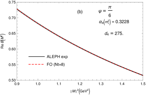
Figure 9: The values of ${\rm Re}B(M^{2};\sigma_{\rm m})$ along the ray $M^{2}=|M^{2}|\exp(i\Psi)$ with $\Psi=\pi/6$. The narrow grey band are the experimental predictions. The red dashed line inside the band is the result of the FOPT global fit with truncation index $N_{t}=8$. Similar fitting curves are obtained for the rays with $\Psi=0$ and $\Psi=\pi/4$.

The truncation index $N_{t}$ is then fixed by considering the first two double-pinched momenta $a^{(2,0)}(\sigma_{\rm m})$ and $a^{(2.1)}(\sigma_{\rm m})$ and requiring local stability of their values under the variation of $N_{t}$. The resulting extracted values of the coupling are

$$\alpha_{S}(m_{\tau}^{2})^{\rm(FO)} = 0.3228\pm 0.0003({\rm exp})^{-0.0026}_{+0.0070}(\kappa)^{-0.0103}_{+0.0079}(d_{4})^{+0.0081}_{-0.0057}(N_{t})$$ (65)

$$= 0.3228^{+0.0134}_{-0.0121}\approx 0.323^{+0.013}_{-0.012}\qquad(N_{t}=8^{+2}_{-3}).$$

$$\alpha_{S}(m_{\tau}^{2})^{\rm({\widetilde{\rm FO}})} = 0.3209\pm 0.0003({\rm exp})^{-0.0038}_{+0.0201}(\kappa)^{-0.0039}_{+0.0047}(d_{4})^{+0.0293}_{-0.0084}(N_{t})$$ (66)

$$= 0.3209^{+0.0359}_{-0.0100}\approx 0.321^{+0.036}_{-0.010}\qquad(N_{t}=5\pm 2).$$

$$\alpha_{S}(m_{\tau}^{2})^{\rm(PV)} = 0.3269\pm 0.0003({\rm exp})^{+0.0007}_{+0.0102}(\kappa)^{-0.0064}_{+0.0155}(d_{4})^{+0.0092}_{-0.0006}(N_{t})^{+0.0167}_{-0.0067}({\rm amb})$$ (67)

$$= 0.3269^{+0.0266}_{-0.0093}\approx 0.327^{+0.027}_{-0.009}\qquad(N_{t}=8^{+2}_{-3}).$$

$$\alpha_{S}(m_{\tau}^{2})^{\rm(CI)} = 0.3488\pm 0.0005({\rm exp})^{+0.0078}_{+0.0004}(\kappa)\pm 0.0000(d_{4})^{-0.0027}_{+0.0119}(N_{t})$$ (68)

$$= 0.3488^{+0.0142}_{-0.0028}\approx 0.349^{+0.014}_{-0.003}\qquad(N_{t}=4^{+2}_{-1}).$$

The uncertainties are presented as separate terms. The variation of the renormalisation scale parameter $\kappa\equiv\mu^{2}/Q^{2}$ was taken in the range $2/3\leq\kappa\leq 2$ ($\kappa=1$ for the central values). The truncation index is $N_{t}=8,5,8$ for the central cases of FO, ${\widetilde{\rm FO}}$ and PV.

The (truncated) Contour improved perturbation theory (CIPT) results are also included in the above results, for comparison. However, the truncated CIPT approach for $d(Q^{2})_{D=0}$ evaluation appears to require a different type of OPE in the $D>0$ part of the contributions, because the renormalon structure and the related renormalon ambiguities are not reflected in the truncated CIPT series Hoang:2021nlz . We thus include only FO, ${\widetilde{\rm FO}}$ and PV results in the average

$$\alpha_{S}(m_{\tau}^{2}) = 0.3235^{+0.0138}_{-0.0126}\qquad({\rm FO}+{\widetilde{\rm FO}}+{\rm PV})$$

$$\Rightarrow\;\alpha_{S}(m^{2}_{\mathrm{Z}}) = 0.1191\pm 0.0016.$$ (69)

In Table 6 we compare these results with some other results in the literature.

Table 6: $\alpha_{S}(m_{\tau}^{2})$ values extracted by various groups from ALEPH $\tau$-decay data applying sum rules and other methods.

group	sum rule	FO	CI	PV	average
Baikov et al., 2008 Baikov:2008jh	$a^{(2,1)}=r_{\tau}$	$0.322\pm 0.020$	$0.342\pm 0.011$	—	$0.332\pm 0.016$
Beneke&Jamin, 2008 Beneke:2008ad	$a^{(2,1)}=r_{\tau}$	$0.320^{+0.012}_{-0.007}$	—	$0.316\pm 0.006$	$0.318\pm 0.006$
Caprini, 2020 Caprini:2020lff	$a^{(2,1)}=r_{\tau}$	—	—	$0.314\pm 0.006$	$0.314\pm 0.006$
Davier et al., 2013 Davier:2013sfa	$a^{(i,j)}$	$0.324$	$0.341\pm 0.008$	—	$0.332\pm 0.012$
Pich&R.Sánchez, 2016 Pich:2016bdg	$a^{(i,j)}$	$0.320\pm 0.012$	$0.335\pm 0.013$	—	$0.328\pm 0.013$
Boito et al., 2014 Boito:2014sta	DV in $a^{(i,j)}$	$0.296\pm 0.010$	$0.310\pm 0.014$	—	$0.303\pm 0.012$
our prev. work, 2021 Ayala:2021mwc	BL ($O_{6},O_{8}$)	$0.308\pm 0.007$	—	$0.316^{+0.008}_{-0.006}$	$0.312\pm 0.007$
this work, 2022 (also Ayala:2021yct )	BL ($O_{6}^{(1)},O_{6}^{(2)}$)	$0.323^{+0.013}_{-0.012}$(FO)	—	$0.327^{+0.027}_{-0.009}$	$0.324\pm 0.013$
		$0.321^{+0.021}_{-0.030}$(${\widetilde{\rm FO}}$)

The results Eq. (69) can get significantly affected when the assumptions or methods are changed. For example, if we chose, instead of the central value $d_{4}=275.$, the upper upper bound $d_{4}=338.$ of Eq. (63) as the central value, the results would decrease somewhat, to $\alpha_{S}(m_{\tau}^{2})\approx 0.320\pm 0.015$ [$\alpha_{S}(m^{2}_{\mathrm{Z}})\approx$ $0.1187^{+0.0016}_{-0.0019}$], i.e., $\delta\alpha_{S}(m^{2}_{\tau})\approx-0.004$. If we took, instead of the two mentioned $D=6$ terms in the OPE, the simple $D=6$ and $D=8$ OPE terms [$\sim 1/(Q^{2})^{3}$ and $\sim 1/(Q^{2})^{4}$], the central value would decrease by about $\delta\alpha_{S}(m^{2}_{\tau})\approx-0.008$. In our previous work Ayala:2021mwc we used the OPE with simple $D=6,8$ terms, and took for $d_{4}$ higher values $d_{4}=338\pm 63$ than here Eq. (63). If we took $N_{t}=5$ in all three methods (i.e., no extension of Adler function beyond $d_{4}a^{5}$), then the central value of $\alpha_{S}(m_{\tau}^{2})$ in FO changes from $0.3288$ to $0.3171$, and in PV from $0.3269$ to $0.3277$ $\Rightarrow$ for the average of the three methods the central value changes from $0.3235$ to $0.3219$ [$\alpha_{S}(m^{2}_{\mathrm{Z}})$ from $0.1191$ to $0.1189$], i.e., $\delta\alpha_{S}(m^{2}_{\tau})=-0.0016\approx-0.002$, small.

According to the results (65)–(67), Borel–Laplace sum rules indicate that the theoretical uncertainties dominate over the experimental ones. Part of these theoretical uncertainties would be reduced by: (1) the calculation of the five-loop Adler function coefficient $d_{4}$; (2) the use of the more complicated structure of the $D=6$ OPE terms Boito:2015joa and the corresponding terms in the $D=0$ $u=3$ IR renormalon structure; (3) the use of a variant of the QCD coupling $a(Q^{2})$ without the Landau singularities in the $D=0$ contribution, because this would allow for the resummation to all orders (no truncation) of the renormalon-motivated contribution $D=0$ and would eliminate the renormalisation scale ambiguity ($\kappa$). The high precision ALEPH determination of the $\tau$ spectral function represents an important source of data for understanding better the behaviour of QCD at the limit between the perturbative and nonperturbative regimes.

4 Reconciling the fixed order and contour improved perturbative series in hadronic $\tau$ decays.

We propose an approach to reconcile the fixed order (FOPT) and contour improved (CIPT) QCD expansions of hadronic spectral function moments relevant for the precise determination of $\alpha_{S}$ from $\tau$ decays. This is achieved through a simple renormalon-free scheme for the gluon condensate matrix element. The scheme relies on external knowledge about the gluon condensate renormalon norm and is capable of resolving the long-standing discrepancy between FOPT and CIPT predictions, under the assumption that the gluon condensate renormalon gives a sizeable contribution to QCD perturbative coefficients at intermediate orders.

Strong coupling determinations from hadronic $\tau$ decay data are based on weighted integrals of the experimental spectral functions with an upper bound $s_{0}\leq m_{\tau}^{2}$ and to integrals of the QCD Adler function over a closed contour in the complex momentum plane. For the latter one must set the renormalization scale in $\alpha_{S}$ when performing the contour integrals. The two widely used prescriptions are based on FOPT and CIPT. In FOPT, the renormalization scale is fixed at $\mu^{2}=s_{0}$, which leads to a power series in $\alpha_{S}(s_{0})$. In CIPT, the scale is tied to the contour’s momentum variable such that logarithms related to the QCD $\beta$ function are summed, but the resulting series is not any more a power series in $\alpha_{S}$. These expansion methods exhibit a sizeable discrepancy at orders $\mathcal{O}(\alpha_{S}^{4})$ and $\mathcal{O}(\alpha_{S}^{5})$ that is larger than the individual renormalization scale variations: $\alpha_{S}$ determinations based on CIPT tend to yield higher values than those based on FOPT. This discrepancy has been one of the main sources of theory uncertainty in $\alpha_{S}$ from $\tau$ decays.

In Ref. Benitez-Rathgeb:2022yqb we lay the foundation for a possible resolution of the discrepancy. In Refs. Hoang:2020mkw ; Hoang:2021nlz it was suggested that the discrepancy is of infrared (IR) origin and largely dominated by the leading IR renormalon of the massless quark QCD Adler function, associated with the gluon condensate (GC). This entails that, once this renormalon is subtracted from the Adler function’s perturbation series, the two expansion methods should yield more consistent values at intermediate orders, reducing the theoretical uncertainty in the extractions of $\alpha_{S}$.

Our work is based on two premises. First, it is assumed that the GC renormalon gives a sizeable contribution to the Adler function’s perturbative coefficients at intermediate orders ($\mathcal{O}(\alpha_{S}^{3})$ to $\mathcal{O}(\alpha_{S}^{5})$). This assumption can be considered as natural, since the GC represents the leading IR sensitivity. It is also supported by all-order results in the large-$\beta_{0}$ limit and by renormalon models Beneke:2008ad ; Beneke:2012vb built for the Adler function in QCD. Second, our framework relies on the fact that the OPE condensate corrections not only provide nonperturbative corrections but also compensate for the associated factorial renormalon growth of the perturbative series coefficients, thus leading to an unambiguous theoretical description. The first premise is important. If it were not true, the FOPT-CIPT discrepancy problem would be unrelated to IR renormalons and no information on the norm of the GC renormalon could be gained from the known QCD corrections for the Adler function. The second premise is an established characteristics of multiloop QCD calculations in the limit of vanishing IR cutoff, where sensitivities to IR momenta are a cause of QCD perturbation series to be asymptotic. Since this is the common approach for the loop corrections for inclusive quantities based on dimensional regularization and the $\overline{\rm MS}$ scheme for the strong coupling, we call this approach to regularize IR momenta ‘$\overline{\rm MS}$ scheme’ as well. This should not be confused with the $\overline{\rm MS}$ scheme for $\alpha_{S}$, which refers to the regularization of UV momenta. We actually use the strong coupling in the $C$ scheme (for the concrete value $C=0$) Boito:2016pwf , referred to as $\bar{\alpha}_{S}$ below.

In heavy-quark physics, it is well stablished that the leading (linear) IR sensitivity that arises in the pole mass renormalization scheme can be eliminated by switching to short-distance mass schemes Hoang:2020iah ; Beneke:2021lkq . In our work Benitez-Rathgeb:2022yqb (see also Benitez-Rathgeb:2021gvw ) we propose a similar approach for the GC matrix element. We start from the operator product expansion (OPE) for the massless quark Adler function. Using the $\overline{\rm MS}$ scheme (to regularize IR momenta), it can be cast in the form (using $\mu^{2}=-s$ as renormalization scale for the strong coupling)

$$\textstyle D(s)\,=\,\sum_{n=1}^{\infty}\,\bar{c}_{n,1}(\frac{\bar{\alpha}_{S}(-s)}{\pi})^{n}+\frac{C_{4,0}(\bar{\alpha}_{S}(-s))}{s^{2}}\langle\bar{\cal O}_{4,0}\rangle+\sum_{d=6}^{\infty}\frac{1}{(-s)^{d/2}}\sum_{i}C_{d,i}(\bar{\alpha}_{S}(-s))\langle\bar{\cal O}_{d,\gamma_{i}}\rangle\,,$$ (70)

where the first term is the perturbative contribution, and the $1/s$ OPE power corrections, starting from the term with $d=4$, are the nonperturbative corrections. The perturbative coefficients $\bar{c}_{n,1}$ are exactly known up $\mathcal{O}(\alpha_{S}^{4})$ Baikov:2008jh ; Herzog:2017dtz . It is customary to also include an estimate for the $\mathcal{O}(\alpha_{S}^{5})$ coefficient $\bar{c}_{5,1}$ in phenomenological analyses Boito:2014sta ; Boito:2020xli ; Pich:2016bdg ; Ayala:2021mwc . The terms $\langle\bar{\cal O}_{d,\gamma_{i}}\rangle$ are nonperturbative vacuum matrix elements (condensates) and the $C_{d,i}$ are the respective Wilson coefficients which are a power series in $\alpha_{S}(-s)$. The bar over the operator indicates that the condensates are defined in the $\overline{\rm MS}$ scheme (to regularize IR momenta).

The leading $d=4$ OPE power correction arises from the GC and is central to this work. It can be cast in terms of the renormalization scale invariant GC matrix element $\langle\bar{G}^{2}\rangle$ as ($\bar{a}(-s)\,\equiv\,\beta_{0}\,\bar{\alpha}_{S}(-s)/(4\pi)$, $\beta_{0}=11-2n_{f}/3$)

$$\delta D^{\rm OPE}_{4,0}(s)\,=\,\textstyle\frac{1}{s^{2}}\frac{2\pi^{2}}{3}\,[1-\frac{22}{81}\,\bar{a}(-s)]\,\langle\bar{G}^{2}\rangle\,.$$ (71)

Associated with the GC OPE correction is a renormalon singularity in the Borel function of the Adler function (see Benitez-Rathgeb:2022yqb for our notation) that has the form

$$B_{4,0}(u) = \textstyle[1-\frac{22}{81}\,\bar{a}(-s)]\,\frac{N_{4,0}}{(2-u)^{1+4\hat{b}_{1}}}\,,$$ (72)

where $N_{4,0}$ is the Adler function’s GC renormalon norm and $\hat{b}_{1}=\beta_{1}/2\beta_{0}^{2}$, with $\beta_{1}$ being the two-loop QCD $\beta$-function coefficient. This GC renormalon singularity contributes to the Adler function’s perturbative series coefficients $\bar{c}_{n,1}$ in the form

$$\textstyle\delta\hat{D}_{4,0}(s)\,=\,N_{4,0}\,[1-\frac{22}{81}\,\bar{a}(-s)+\ldots]\,{\textstyle\sum_{n=1}^{\infty}}\,r_{n}^{(4,0)}\,\bar{a}(-s)^{n}\,,$$ (73)

where the terms $r_{n}^{(4,0)}=2^{-(n+4\hat{b}_{1})}\Gamma(n+4\hat{b}_{1})/\Gamma(1+4\hat{b}_{1})$ diverge factorially. The use of the $C$-scheme Boito:2016pwf is convenient because the term $1/(2-u)^{1+4\hat{b}_{1}}$ in $B_{4,0}(u)$ and the coefficients $r_{n}^{(4,0)}$ in $\delta\hat{D}_{4,0}(s)$ are exact, i.e. they do not receive any further higher order corrections. The first premise entails that $N_{4,0}$ is sufficiently sizeable, such that the series in $\delta\hat{D}_{4,0}(s)$ makes up for a sizeable contribution in the coefficients $\bar{c}_{n,1}$ at the intermediate orders relevant for phenomenological analyses. In the context of this assumption it has been shown in Refs. Hoang:2020mkw ; Hoang:2021nlz , that the FOPT-CIPT discrepancy can be caused by the diverging Adler function series contributions given in $\delta\hat{D}_{4,0}(s)$.

We now turn to the construction of the renormalon-free (RF) gluon condensate scheme. The RF scheme only deals with the GC renormalon; all other renormalons are strictly unaltered. We start by imposing that the order-dependence of $\langle\bar{G}^{2}\rangle$ that compensates the factorial growth of the coefficients in Eq. (73) is made explicit, while maintaining the generic form of the GC OPE correction in Eq. (71). The relation between the original, order dependent, $\overline{\rm MS}$ GC matrix element and a new renormalon-free GC matrix element, $\langle G^{2}\rangle(R^{2})$, is then

$$\langle\bar{G}^{2}\rangle^{(n)}\,\equiv\,\langle G^{2}\rangle(R^{2})\,-\,R^{4}\,{\textstyle\sum_{\ell=1}^{n}}\,N_{g}\,r_{\ell}^{(4,0)}\,\bar{a}^{\ell}_{R}\,,$$ (74)

where $\bar{a}_{R}\equiv\beta_{0}\,\bar{\alpha}_{S}(R^{2})/(4\pi)$ and we made explicit the order dependence on the left-hand side; $N_{g}$ is the universal GC renormalon norm, related to $N_{4,0}$ by $N_{g}=3N_{4,0}/(2\pi^{2})$. The condensate $\langle G^{2}\rangle(R^{2})$ depends explicitly on the scale $R$, which sets its parametric size to be ${\cal O}(R^{4})$ (instead of ${\cal O}(\Lambda_{\rm QCD}^{4})$ for the $\overline{\rm MS}$ GC $\langle\bar{G}^{2}\rangle^{(n)}$). The scale $R$ plays the role of an IR factorization scale which can in principle be chosen arbitrarily. In practice its value should be chosen smaller, but still of the order of, the typical dynamical scale of the observable of interest to avoid the appearance of (or, equivalently, to sum potentially) large logarithms. The dependence of $\langle G^{2}\rangle(R^{2})$ on $R$ is controlled by an $R$-evolution equation Hoang:2009yr (see Benitez-Rathgeb:2022yqb for its precise form).

From a practical perspective, the $R$ dependence of $\langle G^{2}\rangle(R^{2})$ is somewhat inconvenient. We therefore define, in a second step, a scale-invariant renormalon-free GC matrix element. This is achieved by the addition of a function which obeys the same $R$-evolution equation as $\langle G^{2}\rangle(R^{2})$. This is possible because the $R$-derivative of the subtraction series on the r.h.s. of Eq. (74) is convergent for $n\to\infty$. Such a function is obtained from the Borel sum of the subtraction series, defined through the principal value (PV) prescription:

$$\bar{c}_{0}(R^{2}) \equiv R^{4}\,\,\,{\rm PV}\,{\textstyle\int_{0}^{\infty}\!\frac{{\rm d}u}{(2-u)^{1+4\hat{b}_{1}}}}\,e^{-\frac{u}{\bar{a}_{R}}}\,.$$ (75)

The result for $\bar{c}_{0}(R^{2})$ can be given in closed analytic form Benitez-Rathgeb:2022yqb . We can then define a scale invariant renormalon-free GC matrix element, denoted as $\langle G^{2}\rangle^{\rm RF}$, by

$$\langle G^{2}\rangle(R^{2}) \equiv \textstyle\langle G^{2}\rangle^{\rm RF}+N_{g}\,\bar{c}_{0}(R^{2})\,.$$ (76)

We denote as $\langle G^{2}\rangle^{\rm RF}$ the GC in the ‘RF scheme’. The particular forms of the subtraction series in Eq. (74) and the function $c_{0}(R^{2})$ are our choices to define the RF scheme, but may in principle be chosen differently. In general, the subtraction must have the correct large order behavior to eliminate the factorial divergence of the coefficients $r_{n}^{(4,0)}$, but could have additional convergent contributions. This would then imply a different form for $\bar{c}_{0}(R^{2})$. Moreover, we could also add an additional constant to $\bar{c}_{0}(R^{2})$. The RF scheme entails that the difference between the original $\overline{\rm MS}$ GC and our new scale-independent RF GC, $\langle G^{2}\rangle^{\rm RF}$, is formally $\mathcal{O}(\bar{a}_{R}^{n+1})$. In this sense, the modifications to the GC in our new RF scheme are minimal.

Using Eqs. (76) and (71), it is straightforward to write down the resulting perturbation series for the Adler function in the RF GC scheme. Treating the term proportional to $\bar{c}_{0}(R^{2})$, which is part of the definition of $\langle G^{2}\rangle^{\rm RF}$, like a tree-level contribution, the perturbation series has the form: ($\bar{c}_{n}\equiv 4\bar{c}_{n,1}/\beta_{0}$ for $n=1,2,\ldots$)

$$\hat{D}^{\rm RF}(s,R^{2})=\textstyle\frac{1}{s^{2}}\,[1-\frac{22}{81}\bar{a}(-s)]\,N_{4,0}\,\bar{c}_{0}(R^{2})\,+\,{\textstyle\sum_{n=1}^{\infty}}\,\bar{c}_{n}\,\bar{a}^{n}(-s)\,-\,[1-\frac{22}{81}\,\bar{a}(-s)]\,N_{4,0}\,\frac{R^{4}}{s^{2}}{\textstyle\sum_{n=1}^{\infty}}r_{n}^{(4,0)}\bar{a}^{\ell}_{R}\,.$$ (77)

We stress that it is crucial to reexpand and truncate the perturbative series terms (excluding the $\bar{c}_{0}$ term) coherently, using the strong coupling at a common renormalization scale. Only then the cancellation of the GC renormalon is realized. Our treatment of the ‘tree-level’ term proportional to $\bar{c}_{0}(R^{2})$ entails that the GC OPE correction retains its form of Eq. (71) with $\langle\bar{G}^{2}\rangle$ replaced by $\langle G^{2}\rangle^{\rm RF}$. Furthermore, it is possible to show that the Borel sum of the perturbation series for the RF scheme Adler function $\hat{D}^{\rm RF}(s,R^{2})$ based on the PV prescription (as shown in Eq. (75)) remains the same as that of the original $\overline{\rm MS}$ scheme Adler function $\hat{D}(s)=\sum_{n=1}^{\infty}\bar{c}_{n}\bar{a}^{n}(-s)$ independently of the value of $N_{4,0}$ and the choice for $R$. Variations of $R$ therefore vanish in the limit of larger-order truncations. The value of norm $N_{4,0}$ is an input to the RF scheme that must be supplemented independently.

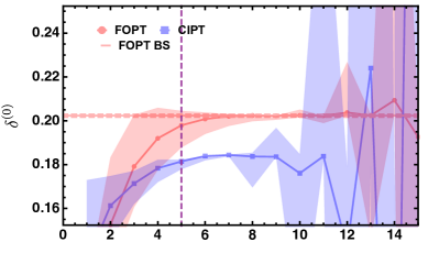
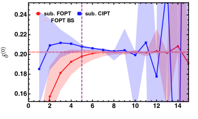
Figure 10: Left: Series for the perturbative FOPT and CIPT expansions of the $\tau$ hadronic decay width order by order in full QCD in the $\overline{\rm MS}$ GC scheme. The orders beyond 5 are obtained from a Borel model. Renormalization scale variations are indicated by the colored bands. Right: Corresponding series for FOPT and CIPT expansions for $\delta^{(0)}_{W}(m_{\tau}^{2},R^{2})$ in the RF GC scheme for $R=0.8\,m_{\tau}$. We use $\alpha_{S}(m_{\tau}^{2})=0.315$ and $n_{f}=3$. The figures are taken from Ref. Benitez-Rathgeb:2022yqb .

Let us now demonstrate the effectiveness of the RF scheme for the perturbation series of the hadronic $\tau$ decay width (see Ref. Benitez-Rathgeb:2022yqb for details). We employ the known QCD corrections up to $\mathcal{O}(\alpha_{S}^{4})$ and use an estimate for the 6-loop coefficient $\bar{c}_{5,1}$, consistent with the values used in the recent analyses Boito:2014sta ; Boito:2020xli ; Pich:2016bdg ; Ayala:2021mwc . We also consider corrections beyond $\mathcal{O}(\alpha_{S}^{5})$ from a renormalon Borel model for the Adler function, based on the works of Beneke:2008ad ; Beneke:2012vb , which has been shown there to be realistic within the first premise mentioned above. The model provides us with the value of $N_{4,0}=4.2$, so that we can study in a concrete way the decay width series in the RF scheme. In the left panel of Fig. 10, we show the results for FOPT (red) and CIPT (blue) in the $\overline{\rm MS}$ scheme for the GC. The vertical dashed line indicates the order up to which we do not rely on the renormalon model. The FOPT and CIPT series exhibit the well-known discrepancy at intermediate orders, which does not diminish with the successive inclusion of higher-order terms predicted by the model. In the context of the first premise, the results show that the discrepancy is systematic and not related to missing higher orders. The two series eventually run into the divergent behavior expected for asymptotic series. The right panel displays the results in the RF GC scheme for $R=0.8\,m_{\tau}$. The FOPT series in the RF scheme is almost unaltered. This can be understood, since the decay width receives only a tiny contribution from the GC through the $s$-dependence of the Wilson coefficient’s 1-loop correction and because the dominant part of the subtraction series in FOPT remains real-valued and factors out of the contour integral. The CIPT series, however, changes dramatically. This is because the subtraction series needs to be expanded according to the CIPT prescription such that the contour integration modifies the contributions from the subtraction series in a nontrivial way. The fact that the resulting numerical effect is so large, corroborates the suggestion of Refs. Hoang:2020mkw ; Hoang:2021nlz that the CIPT series (in the $\overline{\rm MS}$ GC scheme) is not compatible with the generic form of OPE corrections shown in Eq. (70). Remarkably, in the RF scheme the discrepancy between the two series diminishes order by order and at $\mathcal{O}(\alpha_{S}^{5})$ it is already significantly reduced. For even higher orders, the two series become fully compatible and approach essentially the same value. The same observations are made for any other spectral function moment with a suppressed GC. At the same time, the convergence of the perturbation series for moments with an enhanced GC is substantially improved.

Our results show the effectiveness of the new RF GC scheme and provide optimistic prospects that the long-standing FOPT-CIPT discrepancy problem can be resolved. Gaining reliable information on the GC renormalon norm $N_{g}$ remains an important subject of further theoretical investigations.

Acknowledgments— DB and MJ would like to thank the Particle Physics Group of the University of Vienna for hospitality. We acknowledge partial support by the FWF Austrian Science Fund under the Doctoral Program “Particles and Interactions” No. W1252-N27 and under the Project No. P32383-N27. DB’s work was supported by the Coordenação de Aperfeiçoamento de Pessoal de Nível Superior – Brasil (CAPES) – Finance Code 001 and by the São Paulo Research Foundation (FAPESP) Grant No. 2021/06756-6.

IV $\alpha_{S}(m^{2}_{\mathrm{Z}})$ from DIS and parton densities

1 $\alpha_{S}(m^{2}_{\mathrm{Z}})$ through scheme-invariant evolution of N³LO non-singlet structure functions

We describe the measurement of the strong coupling constant $\alpha_{S}(m^{2}_{\mathrm{Z}})$ based on the scheme invariant evolution of unpolarized and polarized flavor non-singlet structure functions at N³LO at an accuracy of the subpercent level. Measurements of this kind can be performed at future facilities such as the EIC and LHeC, provided both proton and deuteron targets are used. The theory framework for this is already available. The measurement requires excellent control of the experimental systematics.

Currently, the values of the strong coupling constant $\alpha_{S}(m^{2}_{\mathrm{Z}})$ as determined in different classes of measurement and even inside these classes is obtained at different values, differing by several standard deviations Proceedings:2011zvx ; Alekhin:2016evh ; Moch:2014tta , reaching an individual accuracy of $\sim$1%. One reason for this lies in the experimental systematics but also in different theoretical approaches being applied. We will consider the measurement of $\alpha_{S}(m^{2}_{\mathrm{Z}})$ using deep-inelastic scattering (DIS) data. To minimize theoretical uncertainties, the measurement method has to be as simple as possible and widely free of effects which are difficult to control or are even widely unknown. Usually one performs mixed twist-2 flavor non-singlet/singlet analyses on a wide host of DIS and other hard scattering data, which are required because besides the flavor non-singlet parton distribution functions those of the different sea quark and gluon distributions are needed as well. Furthermore, the range of $Q^{2}$ usually includes also the region in which higher twist contributions have to be fitted in addition. Also, the treatment of heavy-quark effects varies in the different approaches, although there is no such freedom in general. Some of the cross sections used in the fits may not have the same higher order correction than the massless DIS cross sections. The presence of all these different distribution functions will cost a large part of the statistics power to be determined and various parameter correlations, and potentially introduces theoretical biases, cf. Alekhin:2011sk ; Accardi:2016ndt . This all complicates the measurement of the strong coupling constant in using approaches of this kind.

The situation is completely different in the case of scheme invariant flavor non-singlet evolution of the structure functions $F_{2}^{\rm NS}(x,Q^{2})$ or $g_{1}^{\rm NS}(x,Q^{2})$. The latter structure function usually needs a much higher luminosity, since in addition the longitudinal polarization difference has to be carried out. To form the corresponding data sets, DIS off proton and deuteron targets has to be measured and a reliable description of the deuteron wave function effects is needed. In both cases the input distribution is a measured structure function: $F_{2}^{\rm NS}(x,Q_{0}^{2})$ or $g_{1}^{\rm NS}(x,Q_{0}^{2})$, with experimental error bands. Both the shape of these quantities and their experimental uncertainties can be parameterized at sufficient precision, forming the input for the one-dimensional evolution equation Blumlein:2006be . What remains to be determined in the fit of the data for $Q^{2}>Q_{0}^{2}$ is the strong coupling constant $\alpha_{S}(m^{2}_{\mathrm{Z}})$, the precision of which receives also contributions from the experimental uncertainty of the measured input distribution.

In the following we describe the theoretical basis of the scheme invariant measurement of $\alpha_{S}(m^{2}_{\mathrm{Z}})$ and illustrate a few relevant aspects numerically, following Ref. Blumlein:2021lmf , which may be performed in future experiments at EIC Boer:2011fh or the LHeC LHeCStudyGroup:2012zhm . We consider the combination of structure functions

$$F_{2}^{\rm NS}(x,Q^{2})=F_{2}^{p}-\frac{1}{2}F_{2}^{d}=\frac{1}{6}xC_{2}^{\rm NS}(x,Q^{2})\otimes v_{3}(x,Q^{2}),$$ (78)

where $\otimes$ denotes the Mellin convolution, $C_{2}^{\rm NS}(x,Q^{2})$ is the corresponding unpolarized flavor non-singlet Wilson coefficient and

$$v_{3}(x,Q^{2})=u_{v}(x,Q^{2})-d_{v}(x,Q^{2}).$$ (79)

Nor the flavor singlet, gluon or special sea-quark distributions enter the partonic input distribution. However, the different flavors contribute through virtual QCD corrections, including charm an bottom quarks.

The scale evolution of $F_{2}^{\rm NS}(x,Q^{2})$ can be described by an evolution operator $E_{\rm NS}(x,Q^{2})$

$$F_{2}^{\rm NS}(x,Q^{2})=E_{\rm NS}(x,Q^{2},Q_{0}^{2};m_{c},m_{b})\otimes F_{2}^{\rm NS}(x,Q^{2}_{0}),$$ (80)

which reads in Mellin space

$$E_{\rm NS}(Q^{2},Q_{0}^{2}) = \left(\frac{a}{a_{0}}\right)^{-\frac{P_{0}}{2\beta_{0}}}\Biggl{\{}1+\frac{a-a_{0}}{2\beta_{0}^{2}}\biggl{\{}\Bigl{[}1+a^{2}C_{2}^{Q^{2}}-a_{0}^{2}C_{2}^{Q_{0}^{2}}\Bigr{]}\bigl{(}2\beta_{0}^{2}C_{1}-\beta_{0}P_{1}+\beta_{1}P_{0}\bigr{)}-\frac{\bigl{(}a^{2}-a_{0}^{2}\bigr{)}}{4\beta_{0}^{3}}$$

$$\times\bigl{(}2\beta_{0}^{2}C_{1}-\beta_{0}P_{1}+\beta_{1}P_{0}\bigr{)}\Bigl{[}2\beta_{0}^{3}C_{1}^{2}+\beta_{0}^{2}P_{2}-\beta_{0}\beta_{1}P_{1}+\bigl{(}\beta_{1}^{2}-\beta_{0}\beta_{2}\bigr{)}P_{0}\Bigr{]}+\frac{\bigl{(}a^{2}+aa_{0}+a_{0}^{2}\bigr{)}}{3\beta_{0}^{2}}$$

$$\times\Bigl{[}2\beta_{0}^{4}C_{1}^{3}-\beta_{0}^{3}P_{3}+\beta_{0}^{2}\beta_{1}P_{2}+\bigl{(}\beta_{0}^{2}\beta_{2}-\beta_{0}\beta_{1}^{2}\bigr{)}P_{1}+\bigl{(}\beta_{0}^{2}\beta_{3}-2\beta_{0}\beta_{1}\beta_{2}+\beta_{1}^{3}\bigr{)}P_{0}\Bigr{]}+\frac{a-a_{0}}{4\beta_{0}^{2}}\bigl{(}2\beta_{0}^{2}C_{1}$$

$$-\beta_{0}P_{1}+\beta_{1}P_{0}\bigr{)}^{2}+\frac{(a-a_{0})^{2}}{24\beta_{0}^{4}}\bigl{(}2\beta_{0}^{2}C_{1}-\beta_{0}P_{1}+\beta_{1}P_{0}\bigr{)}^{3}-\frac{a+a_{0}}{2\beta_{0}}\Bigl{[}2\beta_{0}^{3}C_{1}^{2}+\beta_{0}^{2}P_{2}-\beta_{0}\beta_{1}P_{1}$$

$$+P_{0}\bigl{(}\beta_{1}^{2}-\beta_{0}\beta_{2}\bigr{)}\Bigr{]}\biggr{\}}+a^{2}C_{2}^{Q^{2}}-a_{0}^{2}C_{2}^{Q_{0}^{2}}-C_{1}\Bigl{[}a^{3}C_{2}^{Q^{2}}-a_{0}^{3}C_{2}^{Q_{0}^{2}}\Bigr{]}+a^{3}C_{3}^{Q^{2}}-a_{0}^{3}C_{3}^{Q_{0}^{2}}\Biggr{\}}.$$

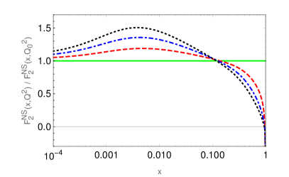
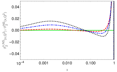
Figure 11: Left: Evolution ratio of the structure function $F_{2}^{\rm NS}(x,Q^{2})$. Right: Relative contribution of the heavy flavor corrections in $F_{2}^{\rm NS}(x,Q^{2})$. Dashed lines: $Q^{2}=10^{2}$ GeV², Dash-dotted lines: $Q^{2}=10^{3}$ GeV², Dotted lines: $Q^{2}=10^{4}$ GeV²; from Ref. Blumlein:2021lmf .

Here $a=a(Q^{2})$ denotes the strong coupling constant and $a_{0}=a(Q^{2}_{0})$, $P_{i}$ are the non-singlet splitting functions and $C_{i}=c_{i}+h_{i}$ the expansion coefficients of the Wilson coefficient, where $c_{i}$ is the massless contribution and $h_{i}$ the massive contribution, where $h_{1}=0,h_{2}=h_{2}^{c}+h_{2}^{b}$ and $h_{3}=h_{3}^{c}+h_{3}^{b}+h_{3}^{cb}$, i.e. there are mixed charm and bottom contributions from three-loops onward, cf. Blumlein:2021lmf for details. The dependence on the heavy-quark mass is logarithmic, with highest logarithmic powers $\ln^{k}(Q^{2}/m_{h}^{2})$ for $h_{k}$. While the non-singlet splitting functions to three-loop order are known Moch:2004pa ; Blumlein:2021enk , the four-loop non-singlet splitting function $P_{3}$ is not yet known, but it can be very well described by a Padé approximation. Eight Mellin moments are known, with the earliest calculation Baikov:2006ai , and the presently available set Moch:2017uml . The massless three-loop Wilson coefficients were calculated in Vermaseren:2005qc and the single and double mass three-loop heavy flavor corrections in Ablinger:2014vwa . At two-loop order the corrections are even available for the whole kinematic region Buza:1995ie ; Blumlein:2016xcy . Different proposals to perform scheme invariant evolution both in the non-singlet and singlet case have been made since 1979, cf. Refs. [92–100] of Ref. Blumlein:2021lmf .

To illustrate the potential of the $\alpha_{S}(m^{2}_{\mathrm{Z}})$ measurement using the present method, we show in Fig. 11 (left) the ratio of $F_{2}^{\rm NS}(x,Q^{2})$ to $F_{2}^{\rm NS}(x,Q^{2}_{0})$ for $Q_{0}^{2}=10$ GeV² up to scales $Q^{2}=10^{4}$ GeV². In the lower $x$ region positive corrections up to a factor of 1.5 are reached, while at large $x$ the corrections are negative. In Fig. 11 (right) we illustrate the impact of the heavy flavor corrections due to charm and bottom quark effects. In the region below $x=0.6$ they are bound to $\pm 1.5\%$ and grow for larger values of $x$. This shows their importance, because the future measurements will be performed at subpercent experimental accuracy. In Ref. Blumlein:2021lmf we also performed related studies for the case of the polarized structure function $g_{1}(x,Q^{2})$.

A precision determination of the strong coupling constant $\alpha_{S}(m^{2}_{\mathrm{Z}})$ requires a high luminosity measurement of a sufficiently simple inclusive observable. The measurement must be carried out under stringent systematic control. Such a measurement would have been possible in the past, if the proposal Guyot:1988 would have been carried out. It has not been possible at HERA, since deuterons have not been probed Alexopoulos:2003aa and the reconstruction of a non-singlet structure function from charged current data has not been precise enough. Given a sufficient preparation, the measurement can be carried out at the EIC using proton and deuteron targets. LHeC may also perform such a measurement, provided also deuteron data will be available and the statistics for the non-singlet measurement is high enough. The theoretical analysis method is then scheme invariant evolution in the flavor non-singlet case for the structure function $F_{2}^{\rm NS}(x,Q^{2})$. Both the light and heavy flavor corrections for this quantity are known on the level of the twist-2 approximation for $Q^{2}\geq 10$ GeV², $W^{2}\geq 15$ GeV², Alekhin:2012ig , to measure $\alpha_{S}(m^{2}_{\mathrm{Z}})$ at an accuracy well below the 1% level. This is one way to decide what is the correct value of $\alpha_{S}(m^{2}_{\mathrm{Z}})$.

To summarize, a high luminosity measurement of $F_{2}^{p}$ and $F_{2}^{d}$ at the EIC would allow to perform the N³LO measurement of $\alpha_{S}(m^{2}_{\mathrm{Z}})$ using the scheme invariant method discussed here.

Acknowledgments— Support from the European Union’s Horizon 2020 research and innovation programme under the Marie Skłodowska-Curie grant agreement No. 764850, SAGEX, is gratefully acknowledged.

2 $\alpha_{S}(m^{2}_{\mathrm{Z}})$ from DIS large-$x$ structure function resummation

We scrutinize the DIS $F_{2}(x,Q^{2})$ structure functions (SFs) measured by the SLAC, NMC and BCDMS experiments Whitlow:1991uw ; Whitlow:1990dr ; Arneodo:1996qe ; Benvenuti:1989rh ; BCDMS:1989ggw ; BCDMS:1987lzs at NNLO accuracy in massless perturbative QCD in order to extract $\alpha_{S}(m^{2}_{\mathrm{Z}})$. The so-called deep-inelastic scattering (DIS) scheme of the SFs Altarelli:1978id is considered, which leads to effective resummation of large-$x$ logarithms into the Wilson coefficient function. The study presented here is a continuation of investigations carried out in closely related papers Shaikhatdenov:2009xd ; Kotikov:2014cua ; Kotikov:2016ljf ; Krivokhizhin:2005pt ; Krivokhizhin:2009zz .

The function $F_{2}(x,Q^{2})$ is represented as a sum of the leading twist (LT) $F_{2}^{\rm pQCD}(x,Q^{2})$ and the twist-four terms (hereinafter, the superscripts pQCD and LT denote the twist-two approximation with and without target-mass corrections):

$$F_{2}(x,Q^{2})=F_{2}^{\rm pQCD}(x,Q^{2})\left(1+\frac{\tilde{h}_{4}(x)}{Q^{2}}\right)\,.$$ (82)

For large $x$ values, gluons do not nearly contribute and the $Q^{2}$ evolution of the twist-two DIS $F_{2}(x,Q^{2})$ SF is well determined by the so-called nonsinglet (NS) part. In this approximation, there is a direct relation between the moments of the DIS $F_{2}(x,Q^{2})$ SF and the moments of the NS parton distribution function ${\bf f}(x,Q^{2})$

$$M_{n}(Q^{2})~{}=~{}\int_{0}^{1}dxx^{n-2}F^{\rm LT}_{2}(x,Q^{2}),~{}~{}{\bf f}(n,Q^{2})~{}=~{}\int_{0}^{1}dxx^{n-1}\,{\bf f}(x,Q^{2})$$ (83)

which can be expressed as follows

$$M_{n}(Q^{2})=R(f)\times C(n,a_{s}(Q^{2}))\times{\bf f}(n,Q^{2})\,,$$ (84)

where the strong coupling constant

$$a_{s}(Q^{2})=\frac{\alpha_{S}(Q^{2})}{4\pi}$$ (85)

and the Wilson coefficient function is denoted as $C(n,a_{s}(Q^{2}))$. The constant $R(f)=1/6$ for $f=4$ Buras:1979yt .

a Strong coupling constant derivation

The strong coupling constant is found from the corresponding renormalization group equation. At the NLO level, $a_{s}^{\rm NLO}(Q^{2})\equiv a_{1}(Q^{2})$, the latter looks like

$$\frac{1}{a_{1}(Q^{2})}-\frac{1}{a_{1}(m_{\mathrm{Z}}^{2})}+b_{1}\ln{\left[\frac{a_{1}(Q^{2})}{a_{1}(m_{\mathrm{Z}}^{2})}\frac{(1+b_{1}a_{1}(m_{\mathrm{Z}}^{2}))}{(1+b_{1}a_{1}(Q^{2}))}\right]}=\beta_{0}\ln{\left(\frac{Q^{2}}{m_{\mathrm{Z}}^{2}}\right)}\,.$$ (86)

At NNLO level, $a_{s}^{\rm NNLO}(Q^{2})\equiv a_{2}(Q^{2})$, the strong coupling constant is derived from the following equation:

$$\frac{1}{a_{2}(Q^{2})}-\frac{1}{a_{2}(m_{\mathrm{Z}}^{2})} + b_{1}\ln{\left[\frac{a_{2}(Q^{2})}{a_{2}(m_{\mathrm{Z}}^{2})}\sqrt{\frac{1+b_{1}a_{2}(m_{\mathrm{Z}}^{2})+b_{2}a_{2}^{2}(m_{\mathrm{Z}}^{2})}{1+b_{1}a_{2}(Q^{2})+b_{2}a_{2}(Q^{2})}}\right]}$$

$$+ \left(b_{2}-\frac{b_{1}^{2}}{2}\right)\times\Bigl{(}I(a_{s}(Q^{2}))-I(a_{s}(m_{\mathrm{Z}}^{2}))\Bigr{)}=\beta_{0}\ln{\left(\frac{Q^{2}}{m_{\mathrm{Z}}^{2}}\right)}\,.$$

The expression for $I$ is

$$I(a_{s}(Q^{2}))=\left\{\begin{array}[]{c}\displaystyle{\frac{2}{\sqrt{\Delta}}}\arctan{\displaystyle{\frac{b_{1}+2b_{2}a_{2}(Q^{2})}{\sqrt{\Delta}}}}\hskip 42.67912pt\mbox{for}~{}~{}f=3,4,5;~{}~{}~{}\Delta>0,\\ \displaystyle{\frac{1}{\sqrt{-\Delta}}}\ln{\left[\frac{b_{1}+2b_{2}a_{2}(Q^{2})-\sqrt{-\Delta}}{b_{1}+2b_{2}a_{2}(Q^{2})+\sqrt{-\Delta}}\right]}~{}~{}\mbox{for}~{}~{}f=6;\hskip 28.45274pt\Delta<0,\end{array}\right.$$

where $\Delta=4b_{2}-b_{1}^{2}$ and $b_{i}=\beta_{i}/\beta_{0}$ are read off from the QCD $\beta$-function:

$$\beta(a_{s})~{}=~{}-\beta_{0}a_{s}^{2}-\beta_{1}a_{s}^{3}-\beta_{2}a_{s}^{4}+\ldots\,.$$

The coefficient function $C(n,a_{s}(Q^{2}))$ is then expressed in terms of the coefficients $B_{j}(n)$, which are exactly known (for the odd $n$ values, $B_{j}(n)$ and $Z_{j}(n)$ can be obtained by using the analytic continuation Kazakov:1987jk ; Kotikov:2005gr ; Kotikov:1994mi )

$$C(n,a_{s}(Q^{2}))=1+a_{s}(Q^{2})B_{1}(n)+a_{s}^{2}(Q^{2})B_{2}(n)+{\cal O}(a_{s}^{3})\,.$$ (88)

The $Q^{2}$-evolution of the PDF moments can be calculated within the framework of perturbative QCD:

$$\frac{{\bf f}(n,Q^{2})}{{\bf f}(n,Q_{0}^{2})}=\left[\frac{a_{s}(Q^{2})}{a_{s}(Q^{2}_{0})}\right]^{\frac{\gamma_{0}(n)}{2\beta_{0}}}\times\frac{h(n,Q^{2})}{h(n,Q^{2}_{0})}\,,$$ (89)

where

$$h(n,Q^{2})=1+a_{s}(Q^{2})Z_{1}(n)+a_{s}^{2}(Q^{2})Z_{2}(n)+{\cal O}\left(a_{s}^{3}\right)\,,$$ (90)

and

$$Z_{1}(n)=\frac{1}{2\beta_{0}}\biggl{[}\gamma_{1}(n)-\gamma_{0}(n)\,b_{1}\biggr{]}\,,~{}~{}Z_{2}(n)=\frac{1}{4\beta_{0}}\left[\gamma_{2}(n)-\gamma_{1}(n)b_{1}+\gamma_{0}(n)(b^{2}_{1}-b_{2})\right]+\frac{1}{2}Z^{2}_{1}(n)\,$$ (91)

are combinations of the NLO and NNLO anomalous dimensions $\gamma_{1}(n)$ and $\gamma_{2}(n)$.

For large $n$ (this corresponds to large $x$ values), the coefficients $Z_{j}(n)\sim\ln n$ and $B_{j}(n)\sim\ln^{2j}n$. So, the terms $\sim B_{j}(n)$ can lead to potentially large contributions and, therefore, should be resummed.

b Scale dependence

We are going to consider the dependence of the results on the factorization $\mu_{F}$ scale caused by (see, e.g., Shaikhatdenov:2009xd ) the truncation of a perturbative series. This way, Eq. (84) takes the form:

$$M_{n}(Q^{2})=R(f)\times\hat{C}(n,a_{s}(k_{F}Q^{2}))\times{\bf f}(n,k_{F}Q^{2})\,.$$

The function $\hat{C}$ is to be obtained from $C$ by modifying the r.h.s. of Eq. (88) as follows:

$$a_{s}(Q^{2}) \to a_{s}(k_{F}Q^{2})\,,~{}~{}B_{1}(n)\to B_{1}(n)+\frac{1}{2}\gamma_{0}(n)\ln{k_{F}}\,,$$

$$B_{2}(n) \to B_{2}(n)+\frac{1}{2}\gamma_{1}(n)\ln{k_{F}}+\left(\frac{1}{2}\gamma_{0}+\beta_{0}\right)B_{1}\ln{k_{F}}+\frac{1}{8}\gamma_{0}\left(\gamma_{0}+2\beta_{0}\right)\ln^{2}{k_{F}}\,.$$ (92)

Taking a special form for the coefficient $k_{F}$, we can decrease contributions coming from the terms $\sim B_{j}(n)$. To accomplish this task, we consider the DIS-scheme Altarelli:1978id , where the NLO corrections to the Wilson coefficients are completely cancelled by changes in the factorization scale.

In the NLO case

$$a_{s}(Q^{2})\to a_{s}(k_{\rm DIS}(n)Q^{2})\equiv a_{n}^{\rm DIS}(Q^{2}),~{}~{}k_{\rm DIS}(n)=\exp\left(\frac{-2B_{1}(n)}{\gamma_{0}(n)}\right)=\exp\left(\frac{-r^{\rm DIS}_{1}(n)}{\beta_{0}}\right)\,,$$ (93)

where

$$r^{\rm DIS}_{1}(n)=\frac{2B_{1}(n)\beta_{0}}{\gamma_{0}}~{}~{}~{}\mbox{and}~{}~{}~{}B_{1}(n)\to B^{\rm DIS}_{1}=0.$$ (94)

The NLO coupling $a^{\rm DIS}_{n}(Q^{2})$ obeys the following equation

$$\frac{1}{a^{\rm DIS}_{n}(Q^{2})}-\frac{1}{a_{1}(m_{\mathrm{Z}}^{2})}+b_{1}\ln{\left[\frac{a^{\rm DIS}_{n}(Q^{2})}{a_{1}(m_{\mathrm{Z}}^{2})}\frac{(1+b_{1}a_{1}(m_{\mathrm{Z}}^{2}))}{(1+b_{1}a^{\rm DIS}_{n}(Q^{2}))}\right]}=\beta_{0}\ln{\left(\frac{Q^{2}}{m_{\mathrm{Z}}^{2}}\right)}-r^{\rm DIS}_{1}(n)\,.$$ (95)

In the NNLO case, in addition to Eqs. (93) and (94) there is also the following modification

$$B_{2}(n)\to B^{\rm DIS}_{2}(n)=B_{2}(n)-\left(\frac{1}{2}+\frac{\beta_{0}}{\gamma_{0}(n)}\right)\,B^{2}_{1}(n)-\frac{\gamma_{1}(n)}{\gamma_{0}(n)}\,B_{1}(n)\,,$$ (96)

that leads to the cancellation of the large terms $\sim\ln^{4}(n)$ in $B^{\rm DIS}_{1}(n)$.

The NNLO coupling $a^{\rm DIS}_{n}(Q^{2})$ obeys the equation

$$\frac{1}{a_{n}(Q^{2})}-\frac{1}{a_{2}(m_{\mathrm{Z}}^{2})} + b_{1}\ln{\left[\frac{a_{n}(Q^{2})}{a_{2}(m_{\mathrm{Z}}^{2})}\sqrt{\frac{1+b_{1}a_{2}(m_{\mathrm{Z}}^{2})+b_{2}a_{2}^{2}(m_{\mathrm{Z}}^{2})}{1+b_{1}a_{n}(Q^{2})+b_{2}a_{n}(Q^{2})}}\right]}$$

$$+\left(b_{2}-\frac{b_{1}^{2}}{2}\right)\times\Bigl{(}I(a_{n}(Q^{2}))-I(a_{s}(m_{\mathrm{Z}}^{2}))\Bigr{)}=\beta_{0}\ln{\left(\frac{Q^{2}}{m_{\mathrm{Z}}^{2}}\right)}-r^{\rm DIS}_{1}(n)\,.$$

c Fit results

Our analysis is carried out for the moments of the $F_{2}(x,Q^{2})$ SF defined in Eq. (83). Then, for each $Q^{2}$, the $F_{2}(x,Q^{2})$ SF is recovered using the Jacobi polynomial decomposition method Parisi:1978jv ; Krivokhizhin:1987rz ; Krivokhizhin:1990ct :

$$F_{2}(x,Q^{2})=x^{a}(1-x)^{b}\sum_{n=0}^{N_{\text{max}}}\Theta_{n}^{a,b}(x)\sum_{j=0}^{n}c_{j}^{(n)}(\alpha,\beta)M_{j+2}(Q^{2})\,,$$ (98)

where $\Theta_{n}^{a,b}$ are the Jacobi polynomials, $a,b$ are the parameters to be fit. The program MINUIT James:1975dr is used to minimize the difference between experimental data and theoretical predictions for the $F_{2}(x,Q^{2})$ SF.

We use free data normalizations for various experiments. As a reference set, the most stable data of hydrogen BCDMS are used at the value of the initial beam energy $E_{0}=200$ GeV. Contrary to previous analyses Shaikhatdenov:2009xd ; Kotikov:2014cua , the cut $Q^{2}\geq$ 2 GeV² is used throughout, since for smaller $Q^{2}$ values Eqs. (95) and (b) have no real solutions.

The starting point of $Q^{2}$-evolution is taken at $Q^{2}_{0}$ = 90 GeV². This value of $Q^{2}_{0}$ is close to the average values of $Q^{2}$ covering the corresponding data. Based on studies done in Ref. Krivokhizhin:2005pt ; Krivokhizhin:2009zz , it is sufficient to take the maximum number of moments $N_{\text{max}}=8$, and the cut $0.25\leq x\leq 0.8$ is applied on the data.

We work within the variable-flavor-number scheme (VFNS) Shaikhatdenov:2009xd . To strengthen the effect of changing the sign of twist-four corrections, we also present results obtained in the fixed-flavor-number scheme with $n_{f}=4$.

Table 7: Parameter values of the twist-four term in different cases obtained in the analysis of data (314 points: $Q^{2}\geq 2$ GeV²) carried out within VFNS (FFNS).

	NLO	NLO	NNLO	NNLO
$x$	$\overline{\mathrm{MS}}$ scheme	DIS scheme	$\overline{\mathrm{MS}}$ scheme	DIS scheme
	$\chi^{2}=246~{}(259)$	$\chi^{2}=238~{}(251)$	$\chi^{2}=241~{}(254)$	$\chi^{2}=242(249)$
	$\alpha_{S}(m^{2}_{\mathrm{Z}})=0.1195$	$\alpha_{S}(m^{2}_{\mathrm{Z}})=0.1177$	$\alpha_{S}(m^{2}_{\mathrm{Z}})=0.1177$	$\alpha_{S}(m^{2}_{\mathrm{Z}})=0.1178$
	(0.1192)	(0.1179)	(0.1170)	(0.1171)
0.275	$-0.245~{}(-0.264)$	$-0.187~{}(-0.174)$	$-0.188~{}(-0.204)$	$-0.141~{}(-0.170)$
0.35	$-0.243~{}(-0.252)$	$-0.111~{}(-0.134)$	$-0.188~{}(-0.193)$	$-0.133~{}(-0.149)$
0.45	$-0.191~{}(-0.187)$	$-0.040~{}(-0.094)$	$-0.172~{}(-0.158)$	$-0.110~{}(-0.104)$
0.55	$-0.116~{}(0.096)$	$-0.106~{}(-0.088)$	$-0.174~{}(-0.137)$	$-0.121~{}(-0.084)$
0.65	0.054 (0.118)	$-0.167~{}(-0.094)$	$-0.145~{}(-0.051)$	$-0.223~{}(-0.100)$
0.75	0.337 (0.477)	$-0.568~{}(-0.442)$	0.115 (0.648)	$-0.587~{}(-0.314)$

As one can see from Table 1, the central values of $\alpha_{S}(m^{2}_{\mathrm{Z}})$ are mostly close to each other upon taking into account total experimental and theoretical errors Shaikhatdenov:2009xd ; Kotikov:2014cua :

$$\pm 0.0022~{}~{}~{}\mbox{(total exp. error)},~{}~{}~{}\left\{\begin{array}[]{c}\displaystyle{+0.0028}\\ \displaystyle{-0.0016}\end{array}\right.~{}~{}~{}\mbox{(theor. error)}\,.$$ (99)

We plan to study these errors in more detail and present them in an upcoming publication.

From Table 1, it can also be seen that after resumming at large $x$ values (i.e. in the DIS scheme), the twist-four corrections change sign at large values of $x$. Thus, unlike the standard analyses performed in Kotikov:2010bm , in this case, when twist-four corrections change the sign, (part of) the powerlike terms can be said to be swallowed up into a QCD analytic constant Shirkov:1997wi just much like as it was observed at low-$x$ values Cvetic:2009kw in the framework of the so-called double asymptotic scaling approach Kotikov:1998qt ; Illarionov:2004nw .

In previous papers Kotikov:1992ht ; Parente:1994bf , where resummation at large values of $x$ was performed within the framework of the Grunberg approach Grunberg:1980ja ; Grunberg:1982fw , we saw only a decrease in the twist-four contribution, since the terms were not studied in detail. That is why we plan to include Grunberg’s approach in an analysis similar to the present one and study in some detail the values of the twist-four corrections.

3 Strong coupling $\alpha_{S}$ in fits of parton distributions

Data from deep-inelastic scattering (DIS) experiments collected during the last few decades contributes significantly to the knowledge about the structure of the proton and the extraction of parton distributions (PDFs). The theory description builds on QCD factorization, which allows to express the structure functions in the charged-lepton- (or neutrino-) proton hard scattering with large momentum transfer $Q$ schematically as

$$F_{a}\,=\,f_{i}\,\otimes\,c_{a,i}\,,\qquad a=2,3,L\,,$$ (100)

where the process-dependent coefficient functions are denoted by $c_{a,i}$ and the PDFs for a given fraction of the proton momentum $x$ by $f_{i\,}(x,\mu^{2})$. Their dependence on the (renormalization and factorization) scale $\mu$ is governed by the well-known evolution equations

$$\frac{\partial}{\partial\ln\mu^{2}}\,f_{i}(x,\mu^{2})\,=\,\left[P_{ik}(\alpha_{S}(\mu^{2}))\otimes f_{k}(\mu^{2})\right]\!(x)\,,$$ (101)

where the standard convolution is abbreviated by $\otimes$. Both, the splitting functions $P_{ik}$ and the coefficient functions by $c_{a,i}$ are calculable in QCD perturbation theory in an expansion in powers of the strong coupling constant $a_{s}\equiv\alpha_{S}(\mu^{2})/(4\pi)$,

$$P\, = a_{s}\,P^{\,(0)}+\,a_{s}^{2}\,P^{\,(1)}+\,a_{s}^{3}\,P^{\,(2)}+\,a_{s}^{4}\,P^{\,(3)}+\,\ldots\,\,,$$ (102)

$$c_{a,i} = c_{a,i}^{\,(0)}+\,a_{s}\,c_{a,i}^{\,(1)}+\,a_{s}^{2}\,c_{a,i}^{\,(2)}\,+\,a_{s}^{3}\,c_{a,i}^{\,(3)}+\,\ldots\,\,.$$ (103)

Here, the first three terms define the NNLO predictions for DIS, which is currently the standard approximation, see Moch:2004pa ; Vogt:2004mw for the splitting functions and vanNeerven:1991nn ; Zijlstra:1992qd ; Zijlstra:1992kj ; Moch:1999eb for the DIS coefficient functions at this accuracy. Form the perturbative expansion in Eqs. (102) and (103) as well as from the PDF evolution in Eq. (101) it is obvious that there is, in general, significant correlations between the PDFs and the value of strong coupling constant $\alpha_{S}(m^{2}_{\mathrm{Z}})$, see e.g. Ref. Accardi:2016ndt . In the ABM PDF fits, this information can be obtained from the (positive-definite) covariance matrix, see, e.g. Alekhin:2017kpj .

Equation (100) holds up to power corrections suppressed by $1/Q^{2}$, and the accessible range of kinematics in the momentum transfer $Q$ and Bjorken $x$ requires careful considerations of the respective kinematic regions. Typical cuts in the application to DIS data restrict the invariant mass of the hadronic system $W^{2}=m_{p}^{2}+Q^{2}(1-x)/x$ (with the proton mass $m_{p}$) to $W^{2}\geq 12.5~{}{\rm GeV}^{2}$ and $Q^{2}\geq 2.5\div 10~{}{\rm GeV}^{2}$, see, e.g. Alekhin:2017kpj . Depending on these cuts, an improved theoretical description of $F_{a}\left(x,Q^{2}\right)$ to account for higher-twist and target-mass corrections becomes necessary. Higher-twist corrections arise from the infinite tower of power corrections $(1/Q^{2})^{n}$, in the operator product expansion (with $n=1,2,3,\dots$). Higher-twist terms have a physical interpretation as multiparton correlations and modify the structure functions in Eq. (100) as

$$F_{a}^{\rm ht}(x,Q^{2}) = F_{a}^{\rm TMC}(x,Q^{2})+\frac{H_{a}^{\tau=4}(x)}{Q^{2}}\,,\qquad\qquad a\,=\,2,T\,,$$ (104)

where the additive terms $H_{a}^{\tau=4}(x)$ models the twist-four contribution and $F_{a}^{\rm TMC}$ denotes the leading twist structure function with target mass corrections, which account for the finite nucleon mass, see, e.g. Alekhin:2017kpj .

Another important aspect in the theoretical description of the leading twist structure functions from Eq. (100) entering in Eq. (104) concerns the active number of flavors and the treatment of DIS heavy quark production Laenen:1992zk A fixed-flavor number scheme and the use the standard decoupling relations for heavy quarks in QCD in the transition from $n_{f}=3$ to $n_{f}=5$ is justified given the currently available kinematics in $x$ and $Q$ for DIS charm quark data, see e.g. Ref. Accardi:2016ndt . Variable-flavor-number schemes attempting the resummation of large logarithms in the ratio $Q^{2}/m^{2}_{h}$ with the heavy-quark mass squared $m^{2}_{h}$ introduce additional theoretical uncertainties from the matching, which manifest themselves predominantly at small $Q^{2}$, see, e.g. Alekhin:2020edf .

The impact of higher twist terms and target mass corrections in Eq. (104) on the extracted value of $\alpha_{S}(m^{2}_{\mathrm{Z}})$ to NNLO accuracy from world DIS data has been illustrated in Fig. 12, where it is shown that variants of the fits with no higher twist lead to systematically larger values of $\alpha_{S}(m^{2}_{\mathrm{Z}})$.

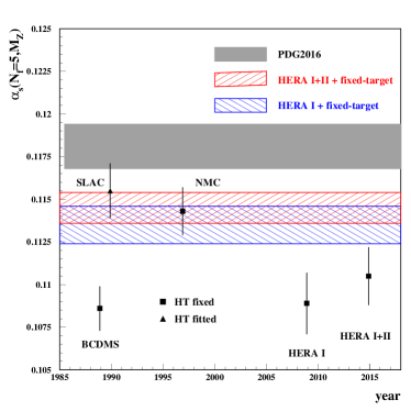
Figure 12: Value of $\alpha_{S}(m^{2}_{\mathrm{Z}})$ in the $\overline{\rm{MS}}$ scheme for $n_{f}=5$ flavors at NNLO in QCD preferred by individual data sets as a function of the year of their publication. Data from SLAC Bodek:1979rx ; Mestayer:1982ba ; Whitlow:1990gk (proton), BCDMS Benvenuti:1989rh , NMC Arneodo:1996qe (proton), the HERA run I Aaron:2009aa as well as the HERA run I+II combination Abramowicz:2015mha are considered in three variants for the treatment of the higher twist terms defined in Eq. (104): (i) the higher twist terms are set to zero (circles); (ii) the higher twist terms are fixed to the values obtained in the ABMP16 fit from considering all data sets (squares); (iii) the higher twist terms are fitted to the individual data set under study (triangles). The bands for $\alpha_{S}(m^{2}_{\mathrm{Z}})$ obtained by using the combination of the SLAC, BCDMS and NMC samples together with those from the HERA run I (left-tilted hatches) and the run I+II combination (right-tilted hatches). The 2016 PDG average Patrignani:2016xqp (shaded area) is shown for comparison. Plot from Ref. Alekhin:2017kpj .

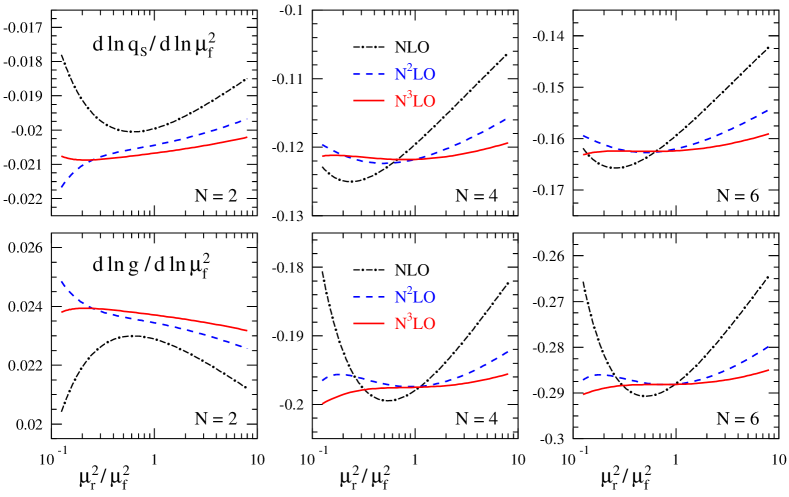
Figure 13: The dependence of the logarithmic factorization scale derivatives of the singlet PDFs on the renormalization scale $\mu_{r}$ at $N=2$ (where the very small scaling violations of $q_{\rm s}$ and $g$ are related by the momentum sum rule), $N=4$ and $N=6$ for $\alpha_{S}(\mu_{0}^{\,2})=0.2$ and $n_{f}=4$ and initial distributions of the form $xq_{\rm s}=0.6\>x^{\,-0.3}(1-x)^{3.5}\,(1+5.0\>x^{\,0.8\,})$ and $xg=1.6\>x^{\,-0.3}(1-x)^{4.5}\,(1-0.6\>x^{\,0.3\,})$ at the standard scale $\mu_{r}=\mu_{f}$. Plot from Ref. Moch:2021qrk .

The combined fit of PDFs and $\alpha_{S}(m^{2}_{\mathrm{Z}})$ to the world data shown in Fig. 12 delivers in the ABMP16 analysis at NNLO in QCD the value of Alekhin:2017kpj

$$\alpha_{S}(m^{2}_{\mathrm{Z}}) = 0.1145\pm 0.0009\,\qquad\text{for}\,n_{f}=5\,,$$ (105)

while the full ABMP16 analysis (also including LHC data on top-quark hadro-production) finds the value

$$\alpha_{S}(m^{2}_{\mathrm{Z}}) = 0.1147\pm 0.0008\,\qquad\text{for}\,n_{f}=5\,.$$ (106)

Higher-order QCD corrections beyond NNLO become important whenever high precision is needed for benchmark processes at the LHC and for the novel accurate DIS measurements expected at the future Electron Ion Collider (EIC). Then, determinations of PDFs and $\alpha_{S}$ at N³LO accuracy requires the calculation of the N³LO corrections in Eqs. (102) and (103). Those for the DIS coefficient functions are already available Vermaseren:2005qc ; Moch:2007gx ; Moch:2007rq ; Moch:2008fj , including effects of massive quarks Ablinger:2014vwa . Work on the four-loop splitting functions in Eq. (102) to ensure QCD evolution equations at N³LO accuracy is ongoing Moch:2017uml ; Moch:2018wjh ; Moch:2021qrk and the gain in the theoretical accuracy in the solution of Eq. (101) for the evolution of the PDFs is illustrated in Fig. 13 for a number of Mellin moments ($N=2$ to $N=6$) available from Ref. Moch:2021qrk . With the full N³LO contributions to DIS the residual theoretical uncertainty due the scale variation and the truncation of the perturbative series will be limited to $1\%$ in the range of parton kinematics relevant for the current world DIS data and the EIC. With respect to the theory error, inclusive DIS data offer the most precise method to measure $\alpha_{S}(m^{2}_{\mathrm{Z}})$.

4 Strong coupling determination in the CT18 global analyses

The CT18 global QCD analysis Hou:2019efy updates the previous CTEQ-TEA PDFs, CT14 Dulat:2015mca and CT14HERA2 Hou:2016nqm , adding a variety of high-precision data from Large Hadron Collider (LHC). New measurements of single-inclusive jet production, Drell–Yan lepton pairs, top-quark pairs, as well as high transverse momentum ($p_{\mathrm{T}}$) of Z bosons from ATLAS, CMS and LHCb, at the center-of-mass energies of 7 and 8 TeV, provide significant additional sensitivity to the PDF determination. A new family of PDF sets, CT18, CT18A, CT18X, and CT18Z, are released at both NLO and NNLO. The nominal PDF set, CT18, is recommended for general collider phenomenology studies, while CT18A includes an additional ATLAS 7 TeV W/Z precision data set ATLAS:2016nqi , which is found to be in tension with other data sets in the global fit. An alternative PDF set, CT18X, has adopted an $x$-dependent DIS scale, which captures the small-$x$ behavior at low $Q^{2}$ and improves the QCD description of HERA DIS data. The CT18Z PDF set includes the features of CT18A and CT18X, in addition to having a slightly larger charm pole mass, $m_{c}=1.4$ GeV versus $m_{c}=1.3$ GeV. CT18Z maximizes the difference from CT18 PDFs, but preserves a similar goodness-of-fit. More details can be found in Ref. Hou:2019efy .

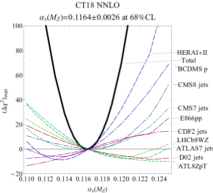
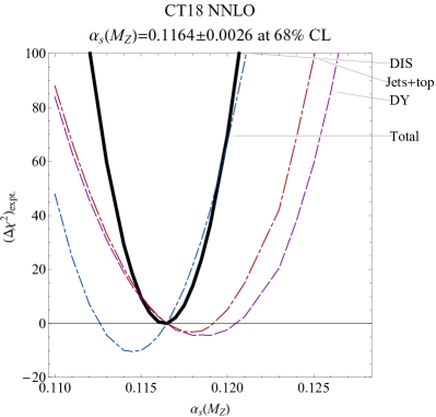
Figure 14: The log-likelihood $\chi^{2}$ in the CT18 NNLO global PDF analysis as a function the strong coupling at scale $m_{\mathrm{Z}}$, plotted for the total fitted data set and the most sensitive experiments. Adapted from Ref. Hou:2019efy .

The final product – the published error PDF sets such as CT18 – takes the strong coupling at a scale $m_{\mathrm{Z}}$ as the world average value $\alpha_{S}(m^{2}_{\mathrm{Z}})=0.118$ ParticleDataGroup:2018ovx . Alternative error PDF sets are produced with a series of fixed $\alpha_{S}(m^{2}_{\mathrm{Z}})$ values for the use in the estimation of combined PDF+$\alpha_{S}$ uncertainties. As shown in CT10 Lai:2010nw , a change in $\alpha_{S}$ is partially compensated by changes in the PDF parameters. An $\alpha_{S}$ uncertainty can be defined, which quantifies the allowed variation of $\alpha_{S}$ when allowed to be freely varied in the PDF fit. In general, the $\alpha_{S}(m^{2}_{\mathrm{Z}})$ sensitivity to a specific data set is introduced either through radiative corrections, such as in the Drell–Yan pair production, or through scaling violations, such as in DIS.

Simultaneous fits of the $\alpha_{S}$ and PDFs were also performed during the CT18 study. An optimal way to explore experimental constraints on $\alpha_{S}(m^{2}_{\mathrm{Z}})$ is to examine the corresponding $\chi^{2}$ variations with the Lagrangian multiplier (LM) technique Stump:2001gu . In Figs. 14, 15 and 16, we adapt this technique to plot a a series of curves for $\Delta\chi^{2}=\chi^{2}(\alpha_{S})-\chi^{2}(\alpha_{S,0})$ for CT18 NNLO, CT18NLO, and CT18Z NNLO, respectively, where $\alpha_{S,0}$ corresponds to the global $\chi^{2}$ minimum in the PDF+$\alpha_{S}$ fit. The black solid curves are for the total $\Delta\chi^{2}$, and the other curves are for $\Delta\chi^{2}$ from the individual experiments with the highest sensitivities to $\alpha_{S}$. From the figures, it is clear that the data sets and even groups of data sets have different preferences to $\alpha_{S}(m^{2}_{\mathrm{Z}})$ in terms of both the central values and uncertainties. The spread of the pulls on $\alpha_{S}$ by the data sets is broader than is would be normally expected from random fluctuations of data around theory, suggesting that a more conservative prescription for the estimation of the $\alpha_{S}$ uncertainty is necessary than the straightforward averaging over the data sets Kovarik:2019xvh .

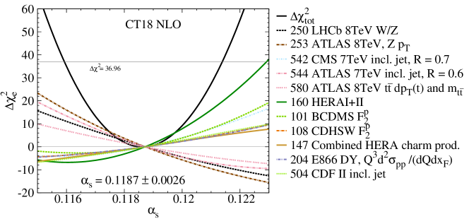
Figure 15: Same as Fig. 14, but now for the $\alpha_{S}(m^{2}_{\mathrm{Z}})$ dependence of $\chi^{2}$ in the CT18 NLO fit. Adapted from Ref. Hou:2019efy .

From the figures, we see that the HERA I and II combined DIS data Abramowicz:2015mha provide the strongest constraints on $\alpha_{S}(m^{2}_{\mathrm{Z}})$ in CT18 at both NLO and NNLO. The BCDMS proton data Benvenuti:1989rh play a slightly stronger role in the CT18Z PDF fit. These two DIS data sets prefer a lower value of $\alpha_{S}(m^{2}_{\mathrm{Z}})$ then the world average, with a value about $0.114\sim 0.116$, but with larger uncertainties. On the other hand, we see that the hadron collider data, such as inclusive jet, top-quark pairs, and Drell–Yan production, pull the $\alpha_{S}(m^{2}_{\mathrm{Z}})$ value higher, with a preferred value of $0.117\sim 0.119$ for the CT18 NNLO case. The strongest pull comes ATLAS 8 TeV Z $p_{\mathrm{T}}$ data ATLAS:2015iiu , followed by the LHCb 8 TeV W/Z measurement LHCb:2015mad . We also see significant pulls from inclusive jet production at ATLAS 7 TeV ATLAS:2014riz and D0 Run II D0:2008nou , as well as the measurements of the $p_{\mathrm{T}}^{t}$ and $m_{t\bar{t}}$ distributions in top-quark pair production at ATLAS 8 TeV ATLAS:2015lsn . In contrast to the ATLAS case, the CMS measurements of inclusive jet production at both 7 TeV CMS:2014nvq and 8 TeV CMS:2016lna prefer a smaller $\alpha_{S}(m^{2}_{\mathrm{Z}})$, reflecting a tension between these measurements from the two experiments.

Within the 68% probability level, the global average values are

$$\alpha_{S}(m^{2}_{\mathrm{Z}})_{\rm NNLO}=0.1164\pm 0.0026,\quad\alpha_{S}(m^{2}_{\mathrm{Z}})_{\rm NLO}=0.1187\pm 0.0026,$$ (107)

while CT18Z NNLO gives $0.1169\pm 0.0027$, all consistent with the world average ParticleDataGroup:2018ovx . In comparison with the CT14 global fit Dulat:2015mca , the CT18 data sets prefer a larger central $\alpha_{S}(m^{2}_{\mathrm{Z}})$ with a marginally smaller uncertainty. Note that the uncertainties quoted here are larger than those in the contemporary analyses done by other two groups, MSHT and NNPDF. This is primarily a result of a more conservative prescription for the uncertainty adopted in CT18, despite similar constraining power of the experiments included by the three groups. The CT18 prescription reflects in part some inconsistency between the fitted data sets, as discussed above. In the presence of such inconsistencies due to unidentified systematic effects, which would lead to enlarged variations in $\alpha_{S}$ when the selection of experimental data sets is varied, the final uncertainty should be generally increased Barlow:2002yb . In addition, the CT18 uncertainty incorporates outcomes from the fits with comparable $\chi^{2}$ that are obtained with more than 250 alternative functional forms of the PDFs and with alternative QCD scale choices in inclusive jet and high-$p_{\mathrm{T}}$ production. To achieve this, the $\alpha_{S}$ and PDF uncertainties are estimated using the tolerance chosen so as to cover a large number of candidate fits that are made with such alternative choices and pass the goodness-of-fit criteria accepted for the final fit Kovarik:2019xvh ; Guzzi:2021fre .

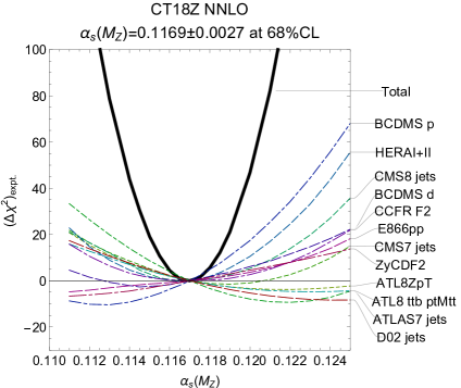
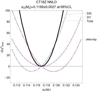
Figure 16: Same as Fig. 14, but for the CT18Z NNLO fit. Adapted from Ref. Hou:2019efy .

Acknowledgments— The work of K.X. is supported by the U.S. Department of Energy, under grant No. DE-SC0007914, U.S. National Science Foundation under Grant No. PHY-2112829, and in part by the PITT PACC. The work of P.N. is supported by U.S. Department of Energy under Grant No. DE-SC0010129.

5 NNLO $\alpha_{S}(m^{2}_{\mathrm{Z}})$ determination from HERA inclusive and jet data

Deep inelastic scattering (DIS) of electrons on protons, e-p, at centre-of-mass energies of up to $\sqrt{s}\approx 320\,$GeV at HERA has been central to the exploration of proton structure and quark–gluon dynamics as described by perturbative Quantum Chromo Dynamics (pQCD). The combination of H1 and ZEUS data on inclusive e-p scattering and the subsequent pQCD analysis, introducing the family of parton density functions (PDFs) known as HERAPDF2.0 Abramowicz:2015mha , was a milestone for the exploitation of the HERA data. The work presented here represents a completion of the HERAPDF2.0 family with a fit at NNLO to HERA combined inclusive data and jet production data published separately by the ZEUS and H1 collaborations. This was not possible at the time of the original introduction of HERAPDF2.0 because a treatment at NNLO of jet production in e-p scattering was not available then.

The name HERAPDF stands for a pQCD analysis within the DGLAP formalism, where predictions from pQCD are fitted to data. These predictions are obtained by solving the DGLAP evolution equations at NNLO in the $\overline{\mathrm{MS}}$ scheme. The inclusive and dijet production data which were already used for HERAPDF2.0Jets NLO were again used for the analysis presented here. A new data set H1:2016goa published by the H1 collaboration on jet production in low $Q^{2}$ events, where $Q^{2}$ is the four-momentum-transfer squared, was added as input to the fits.

The fits presented here were done in the same way as for all other members of the HERAPDF2.0 family, for full details see ZEUS:2021sqd and references therein. All parameter settings were the same as for the HERAPDF2.0Jets NLO fit, with the exception of the heavy quark masses $m_{c}$ and $m_{b}$ and their uncertainty ranges, which were reevaluated using the recently published HERA combined charm and beauty data H1:2018flt . The default minimum $Q^{2}$ of data entering the fit is $Q^{2}=3.5$ GeV² and the starting scale for DGLAP evolution is $Q^{2}_{0}=1.9$ GeV². Note that all HERA data are at very large $W$ so that higher twist effects at small $Q^{2}$ and large $x$ are not relevant.

As for previous HERAPDF analyses, model and parametrisation uncertainties were evaluated. For the present analysis the uncertainties on the hadronisation corrections for the jet data were included as systematic uncertainties, $50\%$ correlated and $50\%$ uncorrelated, together with the experimental systematic uncertainties.

The jet data were included in the fits at NNLO by calculating predictions for the jet cross sections using the NNLOJet Britzger:2019kkb extension of NLOjet++ interfaced to the Applfast framework in order to achieve the speed necessary for iterative PDF fits. The predictions were supplied with uncertainties which were also input to the fit as $50\%$ correlated and $50\%$ uncorrelated systematic uncertainties.

The NNLO analysis of the jet data was applied to a slightly reduced phase space compared to HERAPDF2.0NLOJets. All data points with $\sqrt{\langle p_{\mathrm{T}}^{2}\rangle+Q^{2}}\leq 10$ GeV were excluded to keep the level of scale uncertainties in the predictions for the data points to $\lesssim 10\%$. Six data points, the lowest $\langle p_{\mathrm{T}}\rangle$ bin for each $Q^{2}$ region, were excluded from the ZEUS dijet data set because predictions for these points were not fully NNLO. The trijet data which were used as input to HERAPDF2.0NLOJets had to be excluded as their treatment at NNLO is not available. In addition six extra data points for H1 inclusive jet data at high $Q^{2}$ but low $p_{\mathrm{T}}$, which were published more recently H1:2016goa , were included.

The choice of scales was also adjusted for the NNLO analysis. At NLO, the factorisation scale was chosen as $\mu_{\mathrm{f}}^{2}=Q^{2}$, while the renormalisation scale was linked to the transverse momenta, $p_{\mathrm{T}}$, of the jets by $\mu_{\mathrm{r}}^{2}=(Q^{2}+p_{\mathrm{T}}^{2})/2$. For the NNLO analysis, $\mu_{\mathrm{f}}^{2}=\mu_{\mathrm{r}}^{2}=Q^{2}+p_{\mathrm{T}}^{2}$, was chosen for both factorisation and renormalisation scales.

Jet production data are essential for the determination of the strong coupling constant, $\alpha_{S}(m^{2}_{\mathrm{Z}})$. In pQCD fits to inclusive DIS data alone the value of $\alpha_{S}(m^{2}_{\mathrm{Z}})$ is strongly correlated to the shape of the gluon PDF. Data on jet production cross sections provide an independent constraint on the gluon distribution since inclusive jet and dijet production are directly sensitive to $\alpha_{S}(m^{2}_{\mathrm{Z}})$. Thus such data allow for an accurate simultaneous determination of $\alpha_{S}(m^{2}_{\mathrm{Z}})$ and the PDFs.

The HERAPDF2.0Jets NNLO fit with free $\alpha_{S}(m^{2}_{\mathrm{Z}})$ and $Q^{2}_{\mathrm{min}}=3.5$ GeV² gives a value of

$$\alpha_{S}(m^{2}_{\mathrm{Z}})=0.1156\pm 0.0011\,\mathrm{(exp)}^{+0.0001}_{-0.0002}\,\,\mathrm{(model/parameterisation)}\pm 0.0029\,\mathrm{(scale)}.$$

Note that the the label experimental uncertainty covers the full experimental uncertainties of the simultaneous PDF and free $\alpha_{S}(m^{2}_{\mathrm{Z}})$ fit, which thus includes contributions from the PDF parametrisation, the uncertainty on the hadronisation corrections and the small uncertainties on the theoretical predictions. Additional model uncertainties come from variation of the input assumptions such as the the value of $Q^{2}_{0}$, the starting scale for QCD evolution, the value of the minimum $Q^{2}$ of data entering the fit and the values of heavy quark masses. Additional parametrisation uncertainties come from the consideration of fits which have additional parameters which do not change the $\chi^{2}$ of the fit significantly, but which can sometimes alter PDF shape. A further cross-check on the parametrisation comes from modifying the gluon parametrisation such that it must remain positive definite even at very low-$x$, $x<10^{-4}$, and $Q^{2}$ below $2$ GeV². The largest uncertainty comes from the scale uncertainty, as discussed later.

The HERAPDF2.0Jets NNLO fit with free $\alpha_{S}(m^{2}_{\mathrm{Z}})$ uses 1363 data points and has a $\chi^{2}/$d.o.f. $=1614/1348=1.197$. This can be compared to the $\chi^{2}/$d.o.f. $=1363/1131=1.205$ for HERAPDF2.0 NNLO based on inclusive data only. The similarity of the $\chi^{2}/$d.o.f. values indicates that the data on jet production do not introduce any tension. Data/fit comparisons are shown in Ref. ZEUS:2021sqd

A scan of the fit $\chi^{2}$ for fits with varying $\alpha_{S}(m^{2}_{\mathrm{Z}})$ shown in Fig. 17 and confirms the value of $\alpha_{S}(m^{2}_{\mathrm{Z}})$ and its experimental uncertainty found in the simultaneous $\alpha_{S}(m^{2}_{\mathrm{Z}})$ and PDF fit. The model, parameterisation and scale uncertainties are also shown in the figure. The PDFs associated with this NNLO analysis are described in Ref. ZEUS:2021sqd , the input of the jet data reduces the gluon PDF uncertainties.

Figure 17: Distribution of $\Delta\chi^{2}=\chi^{2}-\chi^{2}_{\mathrm{min}}$ vs. $\alpha_{S}(m^{2}_{\mathrm{Z}})$ for HERAPDF2.0NNLOJets fits with fixed $\alpha_{S}(m^{2}_{\mathrm{Z}})$ values. Experimental, model/parametrisation, and scale uncertainties are illustrated.

The question whether data with relatively low $Q^{2}$ bias the determination of $\alpha_{S}(m^{2}_{\mathrm{Z}})$ arises in the context of the HERA data analysis for which low $Q^{2}$ is also low $x$. A treatment beyond DGLAP may be necessary because of low-$x$ higher-twist terms, $\ln(1/x)$ terms or even parton saturation. To check for such bias the minimum $Q^{2}$ entering the fit was varied to $Q^{2}_{\mathrm{min}}=10$ and $20$ GeV². Thus the HERAPDF analysis considers the possible impact of nonperturbative and beyond DGLAP effects on the result for $\alpha_{S}(m^{2}_{\mathrm{Z}})$. These variations do not alter the value of $\alpha_{S}(m^{2}_{\mathrm{Z}})$ obtained significantly, the value of $\alpha_{S}(m^{2}_{\mathrm{Z}})$ obtained for $Q^{2}_{\mathrm{min}}=10$ GeV² is

$$\alpha_{S}(m^{2}_{\mathrm{Z}})=0.1156\pm 0.0011\,\mathrm{(exp)}\pm 0.0002\,\mathrm{(model/parameterisation)}\pm 0.0021\,\mathrm{(scale)}.$$

The scale uncertainty is reduced with this harder cut on $Q^{2}$ but the largest uncertainty still comes from the scale uncertainty.

The scale uncertainty was evaluated by varying the renormalisation and factorisation scales by a factor of two, both separately and simultaneously (7-point variation), and taking the maximal positive and negative deviations. Scale uncertainties were assumed to be $100\%$ correlated between bins and data sets.

A strong motivation to determine $\alpha_{S}(m^{2}_{\mathrm{Z}})$ at NNLO was the hope to substantially reduce scale uncertainties from those determined at NLO. However, for our previous NLO result we had treated scale uncertainties as 50 % correlated and 50 % uncorrelated. If we repeat this treatment then the scale uncertainty for the present NNLO analysis (with $Q^{2}_{\mathrm{min}}=3.5$ GeV², comparable to the NLO analysis) would be $\pm 0.0022$, very significantly lower than the $+0.0037,-0.0030$ previously observed for the HERAPDF2.0NLOJets analysis. The absolute value of $\alpha_{S}(m^{2}_{\mathrm{Z}})$ at NNLO $\alpha_{S}(m^{2}_{\mathrm{Z}})=0.1156$ is also lower than that observed at NLO $\alpha_{S}(m^{2}_{\mathrm{Z}})=0.1183$. However, the analyses were done at different scales and with somewhat different data sets. In fact, if these choices were harmonised, the difference in the values of $\alpha_{S}(m^{2}_{\mathrm{Z}})$ would be even greater: at NLO $\alpha_{S}(m^{2}_{\mathrm{Z}})=0.1186\pm 0.0014$ (exp) and at NNLO $\alpha_{S}(m^{2}_{\mathrm{Z}})=0.1144\pm 0.0013$ (exp), where the scale choices are both $Q^{2}+p_{\mathrm{T}}^{2}$, the cuts on the data sets for both orders are the harder cuts introduced for the present analysis and the H1 low $Q^{2}$ jet data set H1:2016goa is excluded (this choice is made because these data cannot be well fitted at NNLO). The main reason for the decrease in the central value at NNLO is exclusion of these low-$Q^{2}$ H1 inclusive and dijet data.

It is clear that the main limiting factor today is the theoretical uncertainty, which we estimate from the scale uncertainty. The decrease in scale uncertainty between NLO and NNLO gives some hope for an increase in precision at N³LO. Once theoretical uncertainties are reduced, the experimental uncertainty will need to be reduced. One may hope for progress from analyses at future e-p colliders such as the EIC/LHeC/FCC-eh. Experimental accuracy on $\alpha_{S}(m^{2}_{\mathrm{Z}})\sim 0.0001$ is projected at the LHeC LHeC:2020van .

Acknowledgments— AMC-S would like to thank the Leverhulme Trust.

6 Determination of the strong coupling $\alpha_{S}(m^{2}_{\mathrm{Z}})$ in the MSHT20 NNLO PDF fit

MSHT20 Bailey:2020ooq represented a significant step forward in the global determination of PDFs within the MSHT collaboration (previously MRST/MSTW/MMHT), with more data of greater precision across more channels and more differential in nature now incorporated alongside the inclusion of full NNLO QCD theoretical predictions (and NLO EW corrections where relevant Cridge:2021pxm ). This has been further complemented by progress on the methodological side, including in particular the extension of the PDF parameterisation. The overall result was a significant improvement in our knowledge of the PDFs, including the central values and a general reduction of the PDF uncertainties. Within this context we undertook a follow-up study Cridge:2021qfd examining the effects of varying the strong coupling and heavy quark masses within the global fit. This updated previous work with MMHT14 Harland-Lang:2015nxa . As a result of this new analysis we determined the preferred value of $\alpha_{S}(m^{2}_{\mathrm{Z}})$ and its associated uncertainty and we report on this in this brief review.

The default PDFs within MSHT are provided at $\alpha_{S}(m^{2}_{\mathrm{Z}})=0.118$ at NNLO in order to provide a common value between different PDF fitting groups which is also consistent with the world average value of $\alpha_{S}(m^{2}_{\mathrm{Z}})=0.1179\pm 0.0009$ Zyla:2020zbs . However, $\alpha_{S}(m^{2}_{\mathrm{Z}})$ can also be left as a free parameter and fit alongside the PDFs, we are then able to utilise the global nature of the PDF fits to extract $\alpha_{S}(m^{2}_{\mathrm{Z}})$. Performing the fit with $\alpha_{S}(m^{2}_{\mathrm{Z}})$ free within MSHT20 at NLO and NNLO obtains the best fit values of 0.1203 and 0.1174 respectively, with the excellent quadratic $\chi^{2}$ profiles shown in Fig. 18, demonstrating the clear sensitivity at the global fit level.

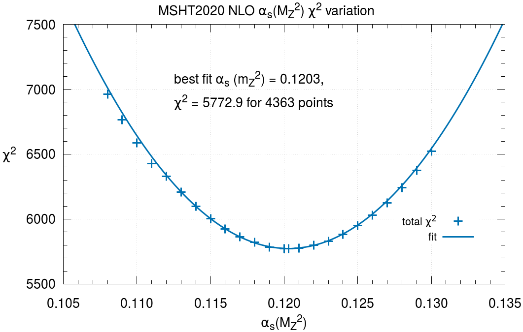
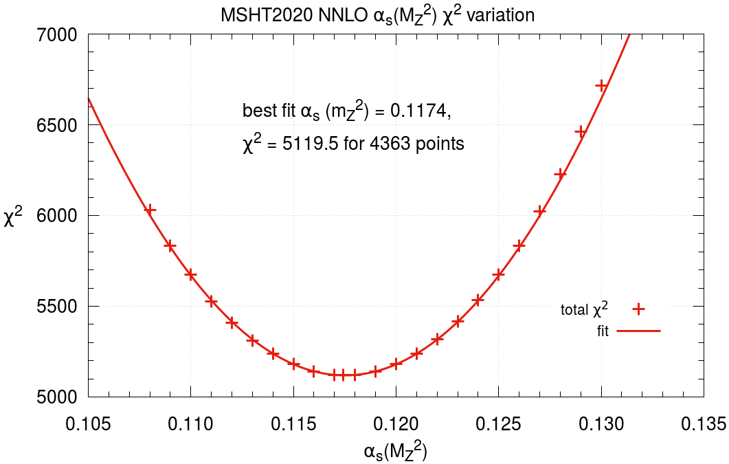
Figure 18: The plots show the total $\chi^{2}$ as a function of $\alpha_{S}(m^{2}_{\mathrm{Z}})$ for NLO (left) and NNLO (right) MSHT20 fits respectively.

Nonetheless, performing such a fit simply extracts the best fit value of the strong coupling, in reality we wish to determine a value of the uncertainty arising on this value from the PDF fit. In order to do this, we utilise the dynamical tolerance method Bailey:2020ooq ; Harland-Lang:2014zoa ; Martin:2009iq which enables the determination of the 68% confidence level interval for the uncertainties on $\alpha_{S}(m^{2}_{\mathrm{Z}})$ by obtaining a “tolerance” $\Delta\chi^{2}$ increase from the best fit value for a particular dataset. Once this is exceeded, it sets the upper and lower bound on a dataset-by-dataset level for the strong coupling. It should be noted this is the same method applied to the determination of the PDF uncertainties. Performing this across the vast array of datasets in MSHT20 one obtains bounds from each dataset on $\alpha_{S}(m^{2}_{\mathrm{Z}})$, the most relevant of which are presented in Fig. 19 for the MSHT20 NNLO fit, further details can be found in Cridge:2021qfd .

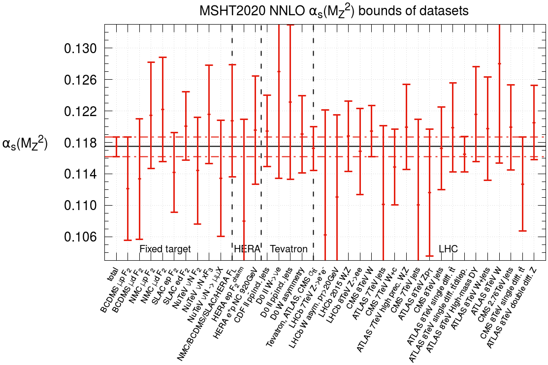
Figure 19: The plot shows the value of $\alpha_{S}(m^{2}_{\mathrm{Z}})$ corresponding to the best fit, together with the upper and lower $1\sigma$ constraints on $\alpha_{S}(m^{2}_{\mathrm{Z}})$ from the more constraining data sets at NNLO. The overall upper and lower bounds taken are given by the horizontal dashed red lines.

As can be observed, different datasets may prefer significantly different values of $\alpha_{S}(m^{2}_{\mathrm{Z}})$ within the context of the global PDF fit and correspondingly offer different bounds. Nonetheless, several general comments can be made. The fixed target and DIS data, and in particular the BCDMS and SLAC proton data, have a preference for lower values of the strong coupling (albeit not universally) in order to slow the fall of the structure function with $Q^{2}$. These represent relatively clean means of determining $\alpha_{S}(m^{2}_{\mathrm{Z}})$ through their high $x$ nature meaning they are dominantly non-singlet. On the other hand, the HERA deep inelastic scattering data has relatively limited sensitivity compared to its large number of points in the fit, this is a reflection of its significant pull on the central values of the PDFs, meaning it naturally sits near the minimum of the profiles. The inclusive jets and Z $p_{\mathrm{T}}$ data from the LHC have direct sensitivity to $\alpha_{S}(m^{2}_{\mathrm{Z}})$ and are seen to generally prefer lower values of the strong coupling within the fit. This is also observed for the top data, certainly at NNLO, however the differential data are dropped from the determination of the global $\alpha_{S}(m^{2}_{\mathrm{Z}})$ bounds due to the fixed top mass available in the theoretical prediction grids utilised, which restricts their utility for the uncertainty determination. Finally, whilst the high precision W, Z data from the LHC have only indirect sensitivity to the strong coupling, these datasets are often still able to provide bounds on $\alpha_{S}(m^{2}_{\mathrm{Z}})$, and are generally seen to favour higher values of $\alpha_{S}(m^{2}_{\mathrm{Z}})$, albeit again not universally.

Examining these bounds on $\alpha_{S}(m^{2}_{\mathrm{Z}})$ across the whole fit, we can then extract the global upper and lower bounds on our strong coupling determinations. At NNLO the BCDMS proton data provides the tightest upper bound, reflecting its preference for a lower $\alpha_{S}(m^{2}_{\mathrm{Z}})$, its $\Delta\chi^{2}$ rises rapidly as the strong coupling is increased and therefore bounds the upward variation of $\alpha_{S}(m^{2}_{\mathrm{Z}})$. On the other hand, the CMS 8 TeV W data provides the most stringent lower bound, fitting with the general trend of the W, Z data favouring larger $\alpha_{S}(m^{2}_{\mathrm{Z}})$ values. Nonetheless, several other datasets would provide only slightly weaker bounds including the SLAC proton data in the upwards direction and the ATLAS 8 TeV Z and high mass Drell–Yan data in the downwards direction. Overall, a symmetrised uncertainty on the strong coupling is obtained of 0.0013, corresponding to a change of $\Delta\chi^{2}_{\rm global}=17$, a similar change in fit quality to that observed for changing the PDFs by their uncertainty in an eigenvector direction. A similar analysis can be performed at NLO, for which the BCDMS proton data again provides the tightest upper bound (followed by the ATLAS 8 TeV Z $p_{\mathrm{T}}$ and ATLAS 7 TeV inclusive jets data, demonstrating their preference for lower $\alpha_{S}(m^{2}_{\mathrm{Z}})$) whilst the LHCb 7 and 8 TeV W,Z data provides the lower bound (closely followed by the SLAC deuterium data). Overall the best fit values and uncertainties on $\alpha_{S}(m^{2}_{\mathrm{Z}})$ within MSHT at NLO and NNLO respectively are determined to be as follows and the NNLO result is consistent with the PDG world average:

$$\alpha_{S}(m^{2}_{\mathrm{Z}})_{\rm NNLO}=0.1174\pm 0.0013,~{}~{}~{}~{}~{}~{}~{}~{}~{}~{}~{}~{}~{}\alpha_{S}(m^{2}_{\mathrm{Z}})_{\rm NLO}=0.1203\pm 0.0015\,.$$

One of the benefits of performing such analyses within the context of global PDF fits, is the incorporation of correlations between the PDFs and the strong coupling, this is investigated in Cridge:2021qfd and the standard method of treating the $\alpha_{S}(m^{2}_{\mathrm{Z}})$ uncertainty as an additional eigenvector in the fit and combining it in quadrature with the PDF uncertainty to obtain the total PDF + $\alpha_{S}(m^{2}_{\mathrm{Z}})$ uncertainty is demonstrated. Given these correlations, there are both direct contributions to the total uncertainty on an observable from the strong coupling change, but also indirect contributions from the associated correlated changes in the PDFs. The latter can partially cancel the direct $\alpha_{S}(m^{2}_{\mathrm{Z}})$ contribution to the uncertainty, for example by probing the gluon below $x\lesssim 0.1$ where it is anticorrelated with the value of the strong coupling. Studies of the heavy quark masses and their correlation with $\alpha_{S}(m^{2}_{\mathrm{Z}})$ were also performed for $m_{\rm charm}$ and demonstrated only limited correlation, with the value of $\alpha_{S}(m^{2}_{\mathrm{Z}})$ extracted rising slightly with the charm quark mass utilised.

The various PDF sets determined within this work are provided for public use on the MSHT website and the LHAPDF repository Buckley:2014ana . In particular, of relevance for this review are the sets provided at NLO and NNLO at fixed $\alpha_{S}(m^{2}_{\mathrm{Z}})$ in steps of 0.001 for the range $0.108\leq\alpha_{S}(m^{2}_{\mathrm{Z}})\leq 0.130$, moreover the $\Delta\chi^{2}_{\rm global}$ in the PDF global fit at each fixed different value of $\alpha_{S}(m^{2}_{\mathrm{Z}})$ in these sets are provided Cridge:2021qfd .

Looking into the future, there are several developments which would facilitate improvements in $\alpha_{S}(m^{2}_{\mathrm{Z}})$ extractions from global PDF fits of deep inelastic scattering and collider data. Firstly, there are questions of the means to incorporate estimates of the theoretical uncertainties into the $\alpha_{S}(m^{2}_{\mathrm{Z}})$ extractions in global PDF fits (beyond relating it to (half) the difference of NLO and NNLO), this is being actively investigated by the various groups and progress is to be expected on this front. Meanwhile, the current uncertainties are limited by the experimental data available, as well as perhaps our understanding of its treatment. The measurements from the LHC in recent years of gluon-sensitive processes, such as inclusive jets and top processes have enabled improvements of our constraints on the PDFs and, in some cases also of $\alpha_{S}(m^{2}_{\mathrm{Z}})$. The rapid availability of grids for theoretical predictions for inclusion in PDFs for $\alpha_{S}(m^{2}_{\mathrm{Z}})$ sensitive processes, such as triple differential jet data, would enable further progress here and this could be complemented by the inclusion of deep inelastic scattering jet data from HERA. The ability to account for the top quark mass dependence in the top differential data would also certainly represent a step forward but is reliant on the provision of theoretical grids at different fixed values, we hope these can be provided in the short term. There is also the possibility of utilising ratios to provide particular sensitivity to $\alpha_{S}(m^{2}_{\mathrm{Z}})$, e.g. the ratio of the inclusive 3- and 2-jet cross-sections CMS:2013vbb , in which the quantities involved are highly correlated (both experimentally and theoretically), these could further supplement the $\alpha_{S}(m^{2}_{\mathrm{Z}})$ sensitivity of the PDFs if included into the global fits. However, more analysis than simply providing the experimental data and corresponding theoretical predictions in a form suitable for inclusion in the PDFs is required. As precision has increased and statistical uncertainties have reduced, systematic uncertainties and their correlations have come to dominate in precision measurements. Correspondingly, increasingly global PDF fits have run into issues with such correlated systematic uncertainties and an improved understanding of such correlations would likely also benefit $\alpha_{S}(m^{2}_{\mathrm{Z}})$ extractions simultaneously to PDF extractions. More broadly, this study emphasises the array of datasets with sensitivity to the strong coupling through the global PDF fits, with older fixed target data providing the tightest bounds in some places and newer LHC inclusive jet and high precision Drell–Yan data providing bounds in others. Therefore the continual evolution of the number and breadth of datasets included, along with their individual precisions, is important for further reducing these uncertainties, and we look forward to further data from the LHC and elsewhere in this regard.

Acknowledgments— T.C. would like to thank the Science and Technology Facilities Council (STFC) for support via grant awards ST/P000274/1 and ST/T000856/1.

7 Strong coupling determinations from the NNPDF global analyses

The model-independent approach based on machine learning which is adopted by the NNPDF Collaboration is specially suitable for the simultaneous extraction of parton distributions together with SM parameters, such as the strong coupling $\alpha_{S}(m^{2}_{\mathrm{Z}})$, the heavy quark masses, and the CKM matrix elements Ball:2009mk as well as BSM parameters such as Wilson coefficients in the Standard Model Effective Field Theory Iranipour:2022iak ; Greljo:2021kvv ; Carrazza:2019sec . In this contribution, we briefly review studies of $\alpha_{S}(m^{2}_{\mathrm{Z}})$ fits in the context of the NNPDF global analyses, and outline ongoing studies in the framework of the NNPDF4.0 determination Ball:2021leu ; NNPDF:2021uiq .

The first determination of the strong coupling in the NNPDF framework was presented in Lionetti:2011pw at NLO and updated in Ball:2011us to NNLO, in both cases based on the NNPDF2.1 dataset and fitting methodology Ball:2011mu ; Ball:2011uy . This dataset contained fixed-target DIS and Drell–Yan data, HERA collider DIS, and gauge boson and jet production measurements from the Tevatron, and hence was devoid of LHC data. A parabolic fit to the $\chi^{2}({\alpha_{S}})$ profile constructed from a large number of uncorrelated Monte Carlo replicas led to a value of the strong coupling

$$\alpha_{S}(m^{2}_{\mathrm{Z}})=0.1173\pm 0.0007_{\rm pdf}\pm 0.0009_{\rm mhou}\,,$$ (108)

at NNLO, where the missing higher order uncertainties (MHOUs) were estimated using the Cacciari–Houdeau method Bagnaschi:2014wea . The stability of this determination with respect to the number of replicas was assessed, and the distribution of pulls from individual datasets was found consistent with statistical expectations.

The extraction of $\alpha_{S}(m^{2}_{\mathrm{Z}})$ within the NNPDF framework was subsequently revisited in Ball:2018iqk , an analysis based on the NNPDF3.1 settings NNPDF:2017mvq . In order to fully account for the PDF- and data-induced correlations on $\alpha_{S}(m^{2}_{\mathrm{Z}})$, a new methodology denoted as the “correlated replica (c-replica) method” was developed. In this approach, one also produces variants of the global fit for different $\alpha_{S}(m^{2}_{\mathrm{Z}})$ values, but in a manner that one has used correlated data- and PDF-replicas which are identical in all settings except for the value of the strong coupling itself. The correlated replica method makes possible a more robust estimate of the methodological uncertainties associated to the $\alpha_{S}(m^{2}_{\mathrm{Z}})$ extraction, at the price of a high computational cost since the number of replicas that need to be generated in this way is $\mathcal{O}(10^{4})$.

Figure 20 (left) displays the NNPDF2.1- and NNPDF3.1-based NNLO determinations of $\alpha_{S}(m^{2}_{\mathrm{Z}})$, compared with the results from the corresponding MMHT14 and ABMP16 analyses as well as to the 2017 PDG average. The thicker error bars correspond to the PDF uncertainties, while the thinner ones indicate the addition in quadrature of PDF and MHO uncertainties. The latter are estimated as half the difference between the NNLO and NLO results. The NNPDF3.1-based NNLO result is found to be

$$\alpha_{S}(m^{2}_{\mathrm{Z}})=0.1185\pm 0.0005_{\rm pdf}\pm 0.0001_{\rm meth}\pm 0.0011_{\rm mhou}\,.$$ (109)

One can observe the good consistency between the two NNPDF determinations among them, as well as with the MMHT14 result and with the PDG average. It is also clear how, specially for the NNPDF3.1-based analysis, MHOUs are currently the limiting factor in strong coupling determinations from global PDF fits. The methodological uncertainties, associated to e.g. the finite number of replicas, are found to be negligible in comparison to both the data and the MHO uncertainties. The role of the choice of figure of merit $\chi^{2}$ was also explored, showing that the frequently used experimental definition leads to a downwards D’Agostini bias which is avoided with the $t_{0}$ definition Ball:2009qv ; Ball:2012wy .

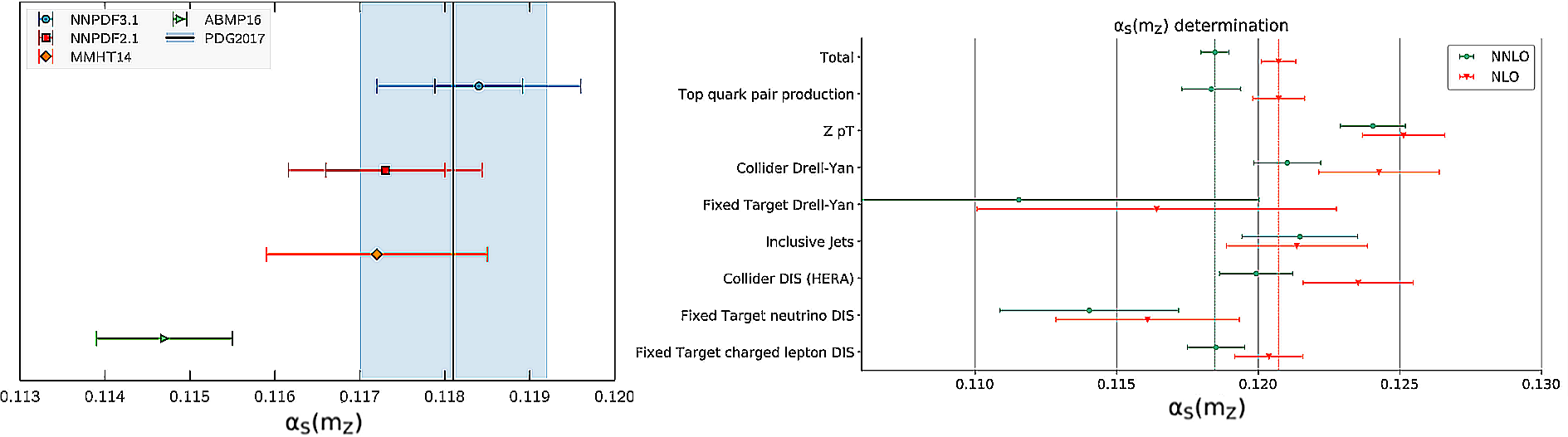
Figure 20: Left: NNPDF2.1- and NNPDF3.1-based NNLO determinations of $\alpha_{S}(m^{2}_{\mathrm{Z}})$, compared with the corresponding results from the MMHT14 and ABMP16 analyses as well as to the 2017 PDG average. The thicker error bars correspond to the PDF uncertainties, while the thinner ones indicate the addition in quadrature of PDF and MHO uncertainties. Right: Central values and 68% CL uncertainties on $\alpha_{S}(m^{2}_{\mathrm{Z}})$ in the NNPDF3.1 NLO and NNLO analyses, comparing the baseline results with those obtained from the partial $\chi^{2}_{p}(\alpha_{S})$ restricted to the specific subsets of processes indicated.

One issue which is frequently raised in the context of PDF-based $\alpha_{S}$ extractions is that of the interplay between the various types of processes that enter the global fit, and whether or not their relative pulls are overall consistent with the global determination. One possible strategy to gain some insight on this is provided by repeating the $\alpha_{S}(m^{2}_{\mathrm{Z}})$ extraction but now using the partial, $\chi^{2}_{p}(\alpha_{S})$, rather than global, $\chi^{2}_{\rm tot}(\alpha_{S})$, profiles. Hence in this case $\alpha_{S}(m^{2}_{\mathrm{Z}})$ is extracted from a $\chi^{2}_{p}(\alpha_{S})$ profile restricted to the contribution of specific groups of processes, i.e. top quark or jet data. It should be emphasised, that, as discussed in detail in Forte:2020pyp , it would not be correct to interpret these results as the value of $\alpha_{S}$ preferred by say top or jet data: such value could only be determined from a PDF fit based exclusively on this specific group of processes. With this caveat, Fig. 20 (right) displays the central values and 68% CL uncertainties on $\alpha_{S}(m^{2}_{\mathrm{Z}})$ in the NNPDF3.1 NLO and NNLO analyses, comparing the baseline results with those obtained from the partial $\chi^{2}_{p}(\alpha_{S})$ restricted to the specific subsets of processes listed. One can observe that collider processes (jets, Z $p_{\mathrm{T}}$, Drell–Yan) tend to favour a larger $\alpha_{S}$ value as compared to the global fit result, while the opposite is found for most fixed-target measurements. The best-fit values from $\chi^{2}_{p}(\alpha_{S})$ for top quark pair production and neutral-current DIS structure functions are similar to the global fit result.

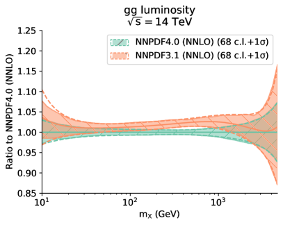
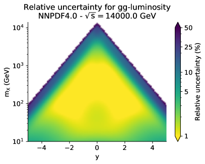
Figure 21: Left: Comparison of the gluon-gluon PDF luminosities at the LHC $\sqrt{s}=14$ TeV as a function of the invariant mass $m_{X}$ between the NNPDF3.1 and NNPDF4.0 NNLO fits, highlighting the impact of the new gluon-sensitive measurements. Right: Relative PDF uncertainties in the double-differential gluon-gluon luminosity as a function of $m_{X}$ and the rapidity $y$ in NNPDF4.0.

Work in progress aims to revisit these $\alpha_{S}(m^{2}_{\mathrm{Z}})$ extractions now based on the recent NNPDF4.0 Ball:2021leu ; NNPDF:2021uiq analysis. NNPDF4.0 benefits from a number of methodological improvements as well as from the addition of several gluon-sensitive measurements, such as dijets AbdulKhalek:2020jut , direct photon production Campbell:2018wfu , and several new top quark production datasets, which in turn provide novel handles on the $\alpha_{S}$ value. The left panel of Fig. 21 compares the gluon-gluon PDF luminosity at the LHC $\sqrt{s}=14$ TeV between the NNPDF3.1 and NNPDF4.0 NNLO fits, highlighting the impact of the new gluon-sensitive measurements both in terms of uncertainty reduction as well as in the shift in central values. The right panel of Fig. 21 displays the percentage PDF uncertainties in the double-differential gluon-gluon luminosity as a function of $m_{X}$ and the rapidity $y$ in NNPDF4.0 NNLO, showing how uncertainties are at the 1% level for most of the kinematic range accessible at the LHC. In order to fully exploit the uncertainty reduction in the PDF determination observed in NNPDF4.0, it will be crucial to assess carefully all other sources of uncertainty that impact the $\alpha_{S}$ extraction of global PDF fit, in particular those associated with MHOUs, which will be tackled using the strategy laid out in NNPDF:2019ubu ; NNPDF:2019vjt .

Future work by the NNPDF collaboration will focus on extending the correlated replica method to the NNPDF4.0 fits and update the determination of the strong coupling constant. Another option that is being considered is the recently developed SIMUnet methodology Iranipour:2022iak , based on an extension of the NNPDF4.0 neural network architecture with an extra layer to simultaneously determine PDFs alongside an arbitrary number of SM and BSM parameters from the direct joint minimisation of the figure of merit $\chi^{2}$. The main advantage of SIMUnet would be to bypass the need of running a very large number of MC replicas, since the simultaneous extraction of $\alpha_{S}(m^{2}_{\mathrm{Z}})$ together with the PDFs would only require $N_{\rm rep}=\mathcal{O}(100)$ replicas as in standard NNPDF fits. Results for the determination of $\alpha_{S}(m^{2}_{\mathrm{Z}})$ from NNPDF4.0 using both SIMUnet and the correlated replica method will be presented in the near future.

8 Measurements of $\alpha_{S}$ from spin structure functions

In this section, we discuss the extraction of $\alpha_{S}$ from nucleon spin structure data. The information is obtained from the cross-section asymmetry of Deep Inelastic scattering (DIS). The cross-section for inclusive lepton scattering is:

$$\frac{d\sigma}{d\Omega\ dx}=\sigma_{\text{Mott}}\big{[}aF_{1}(x,Q^{2})+bF_{2}(x,Q^{2})+cg_{1}(x,Q^{2})+dg_{2}(x,Q^{2})\big{]},$$ (110)

where $\Omega$ is the solid angle, and $\sigma_{\text{Mott}}$, $a$, $b$, $c$ and $d$ are kinematic factors (see e.g. Deur:2018roz for their explicit expressions). In particular, $\sigma_{\text{Mott}}$ is the Mott cross-section for scattering off a point-like target. The information on the nucleon structure is contained in the four structure functions $F_{1}(x,Q^{2})$, $F_{2}(x,Q^{2})$, $g_{1}(x,Q^{2})$ and $g_{2}(x,Q^{2})$. The unpolarized structure functions $F_{1}$ and $F_{2}$ are obtained with unpolarized beam and/or target and are kinematically separated by varying $a$ and $b$. The spin structure functions $g_{1}$ and $g_{2}$ arise when beam and target are both polarized. One accesses $g_{1}$ and $g_{2}$ by measuring beam spin asymmetries. Varying the target polarization direction allows to separate $g_{1}$ from $g_{2}$. One can extract $\alpha_{S}$ from $g_{1}$ ($g_{2}$ is harder to measure and without simple partonic interpretation) by performing a global fit of its $Q^{2}$-evolution, see e.g. Blumlein:2010rn . This is a thorough but complex method, and modeled nonperturbative inputs (quark and gluon PDFs and possibly higher-twists) are required. Alternatively, the $Q^{2}$-evolution of the moment $\Gamma_{1}(Q^{2})\equiv\int_{0}^{1}g_{1}(x,Q^{2})dx$ can be used. The method is much simpler since there is no $x$-dependence, and the nonperturbative inputs are the more-or-less well-measured axial charges $a_{0}$, $a_{3}$ and $a_{8}$ Deur:2018roz (and higher-twists if low-$Q^{2}$ data are used). The difficulty is that the low-$x$ contribution to a moment cannot be measured, as it would require infinite beam energy. Furthermore, $a_{0}$, which is the quark spin contribution to the nucleon spin, is $Q^{2}$-dependent and in some renormalization schemes may receive a contribution from the polarized gluon PDF $\Delta G$. Extracting $\alpha_{S}$ is further simplified when the isovector component of $\Gamma_{1}$ is used, viz, $\Gamma_{1}^{p}-\Gamma_{1}^{n}\equiv\Gamma_{1}^{p-n}$. The relevant axial charge is precisely measured ($a_{3}=g_{A}=1.2762(5)$) Zyla:2020zbs , the $Q^{2}$-evolution of $\Gamma_{1}^{p-n}$ is known to higher order than $\Gamma_{1}^{p,n}$ or $g_{1}$ Kataev:1994gd ; Kataev:2005hv ; Baikov:2010je , and there is no gluon contribution. On the other hand, the low-$x$ issue remains and $\Gamma_{1}^{p-n}$ measurements are demanding since polarized proton and neutron data are needed. We will focus here on using $\Gamma_{1}^{p-n}$.

The Bjorken sum rule Bjorken:1966jh ; Bjorken:1969mm generalized to finite $Q^{2}$ by including QCD radiative and power corrections is Kataev:1994gd ; Kataev:2005hv ; Baikov:2010je :

$$\vspace{-0.2cm}\Gamma_{1}^{p-n}(Q^{2})=\frac{g_{A}}{6}\bigg{[}1-\frac{\alpha_{S}}{\pi}-3.58\left(\frac{\alpha_{S}}{\pi}\right)^{2}-20.21\left(\frac{\alpha_{S}}{\pi}\right)^{3}-175.7\left(\frac{\alpha_{S}}{\pi}\right)^{4}-\sim 893\left(\frac{\alpha_{S}}{\pi}\right)^{5}+\mathcal{O}(\alpha_{S}^{6})\bigg{]}+$$

$$\frac{M^{2}}{Q^{2}}\big{(}a_{2}+4d_{2}+4f_{2}\big{)}+\mathcal{O}(1/Q^{4}),$$ (111)

where the series coefficient values are for $\overline{\mathrm{MS}}$ and $n_{f}=3$. Here, $M^{2}$ is nucleon mass, $a_{2}(Q^{2})$ and $d_{2}(Q^{2})$ are the twist-2 and 3 target mass corrections, respectively, and $f_{2}(Q^{2})$ is the dynamical twist-4 correction. The higher twist coefficients are also subject to QCD radiative corrections and thus depend on $\alpha_{S}$, i.e. $Q^{2}$. To extract $\alpha_{S}$, one can either solve Eq. (111) for $\alpha_{S}$ or fit the $Q^{2}$-dependence of Eq. (111). The latter method is more accurate because it suppresses systematic uncertainties affecting the magnitude of $\Gamma_{1}^{p-n}$ Altarelli:1996nm . We performed such analysis on the data of the Jefferson Lab (JLab) experiment EG1dvcs  CLAS:2015otq ; CLAS:2017qga . The experiment took data during the 6 GeV era of JLab and used the CEBAF Large Acceptance Spectrometer (CLAS) together with polarized NH₃ (for proton) and ND₃ (for neutron) targets and the JLab polarized electron beam. Since EG1dvcs was dedicated to exclusive measurements (DVCS process) it provides inclusive data with very high statistics. We used EG1dvcs data solely to avoid uncorrelated systematics between different experiments since, in contrast to point-to-point correlated systematics (e.g. from polarimetries), uncorrelated errors are not suppressed in the extraction of $\alpha_{S}$. Furthermore, since the EG1dvcs data largely dominate the world data in terms of statistics, including other experiments would only increase the systematic uncertainty on the extraction without being balanced by the gains in $Q^{2}$ leverage and statistics. However, one must recognize that the availability of polarized $g_{1}$ data from higher energy experiments E143:1998hbs ; E142:1996thl ; E154:1997xfa ; E155:1999pwm ; E155:2000qdr ; SpinMuon:1993gcv ; SpinMuonSMC:1997voo ; SpinMuonSMC:1994met ; SpinMuon:1995svc ; SpinMuonSMC:1997ixm ; SpinMuonSMC:1997mkb ; COMPASS:2005xxc ; COMPASS:2006mhr ; COMPASS:2010wkz ; HERMES:1997hjr ; HERMES:1998cbu ; HERMES:2006jyl ; Deur:2004ti ; Deur:2008ej is crucial for this analysis since it allows to control the low-$x$ extrapolation necessary to complement $\Gamma_{1}^{p-n}$. We used the 5 data points of EG1dvcs for which $Q^{2}>2.32$ GeV². The statistical uncertainty is negligible for this analysis. We separated the point-to-point correlated uncertainty from the point-to-point uncorrelated one using the unbiased estimate prescription Schmelling:1994pz ; Zyla:2020zbs , and approximately separated the uncertainties on the low-$x$ extrapolation into $Q^{2}$-dependent and independent parts. Thus, a large fraction of the uncertainties is suppressed in the extraction of $\alpha_{S}$. The dominant errors are the point-to-point uncorrelated (4.4%) and correlated (3.3%) uncertainties. The others are negligible (power corrections: $<$0.1$\%$; Eq. (111) truncation: 1.3%; truncation of the $\beta$-series needed to evolve $\alpha_{S}$ to $m_{\mathrm{Z}}$: 0.1%). In all we obtained $\alpha_{S}(m^{2}_{\mathrm{Z}})=0.1123\pm 0.0061$ Deur:2014vea at N³LO with an N⁴LO correction estimate, see Eq. (111).

Two developments can improve this analysis. The first is experiment EG12 using CLAS12 with the JLab 11 GeV beam and scheduled for June 2022. The expected precision is similar to EG1dvcs, but with a $Q^{2}$ reach of up to 6 GeV and better low-$x$ coverage. The second is the EIC Accardi:2012qut , which we will now summarily investigate.

The optimal $Q^{2}$ range to extract $\alpha_{S}$ from $\Gamma_{1}^{p-n}$ at EIC is $1\lesssim Q^{2}\lesssim 50$ GeV². Below, power corrections could be an issue and above, the unmeasured low-$x$ part of $\Gamma_{1}^{p-n}$ becomes large ($\gtrsim$15%. Since for EIC there will be no higher energy data to guide the low-$x$ extrapolation, it must be kept small). Assuming a luminosity of 2$\times$$10^{33}$cm²s^-1 and an electron (nucleus) beam polarization of 50% (60%), a year of data taking yields statistics ranging from $\Delta\Gamma_{1}^{p-n}=0.5\%$ for $Q^{2}=3$ GeV² to $0.05\%$ for $Q^{2}=15$ GeV². For systematics we assume 4% for deuteron’s nuclear corrections or negligible if the associated proton can be tagged, 100% on the low-$x$ extrapolation, 3% on beam polarimetries, 6% on radiative corrections, 2.5% on the $F_{1}$ structure function necessary to form $g_{1}$ from the measured $A_{1}$ asymmetry Deur:2018roz (specifically, we assumed 2% on $F_{2}$ and 10% on the $R$ ratio). Since $g_{2}$ will be measured at the EIC, correcting for it to obtain $A_{1}$ from the experimental asymmetry $A_{||}$ will not add significant uncertainties. We neglected the contamination from particle misidentification. Detector/trigger efficiencies, acceptance, beam currents uncertainties are negligible for asymmetry measurements. Finally, we assumed that 60% of the systematic is point-to-point uncorrelated, as found for the EG1dvcs data. Fitting the simulated pseudo-data yields $\Delta\alpha_{S}(m^{2}_{\mathrm{Z}})=\pm 0.0033\pm 0.0005$, where the first (second) uncertainty is point-to-point uncorrelated (correlated). The fit was performed over $1.5\leq Q^{2}\leq 15$ GeV². Adding a higher $Q^{2}$ data point only reduces marginally the point-to-point uncorrelated error while significantly increasing the correlated one: $\Delta\alpha_{S}(m^{2}_{\mathrm{Z}})=\pm 0.0030\pm 0.0021$. Increasing the statistics by a factor of 10 and assuming that the proton of the deuteron can be tagged yields $\Delta\alpha_{S}(m^{2}_{\mathrm{Z}})=\pm 0.0016\pm 0.0003$. This simple exercise suggests that an accurate measurement of acceptable precision is possible at EIC, warranting to investigate more seriously the possibility.

Finally, we describe another extraction of $\alpha_{S}$ from $\Gamma_{1}^{p-n}$ at low $Q^{2}$. It uses the gauge-gravity duality, specifically LFHQCD Brodsky:2014yha , a model closely tied to QCD. The Lagrangian of LFHQCD is that of QCD quantized on the light-front, a completely rigorous procedure. The only unknown is the interaction part of the Lagrangian. It can be determined by imposing the approximate chiral symmetry of QCD. Alternatively, one can require QCD’s approximate conformal symmetry and apply de Alfaro–Fubini–Furlan procedure deAlfaro:1976vlx , or require that the light-front potential transformed to the traditional instant-form produces the Cornell potential in the heavy quark case Trawinski:2014msa . The three methods lead to the same semiclassical potential that effectively accounts for the action of the gluons. Imposing upon LFHQCD a nearly exact QCD symmetry to determine the full Lagrangian is the same procedure as used for chiral perturbation theory to determine its Lagrangian. However, contrary to the latter, no counterterms determined from phenomenology are required for LFHQCD since renormalization is unnecessary for nonperturbative frameworks. In fact, LFHQCD has in principle a single free parameter, determined e.g. from a hadron mass or a fit to the $\Gamma_{1}^{p-n}(Q^{2})$ data at low $Q^{2}$. (One free parameter is always needed to set units since they are arbitrary human conventions.) In practice, LFHQCD has a few additional parameters to account for hadronic higher Fock states. They are however of secondary importance and do not enter the determination of $\alpha_{S}$ discussed here. LFHQCD provides a wide range of results that agree with experiments, including hadron spectroscopy Deur:2014qfa , form factors Sufian:2016hwn , polarized and unpolarized PDFs and GPDs deTeramond:2018ecg ; deTeramond:2021lxc ; Liu:2019vsn and $\alpha_{S}(Q^{2})$ Brodsky:2010ur . The latter is obtained by forming the effective charge Grunberg:1980ja ; Grunberg:1982fw ; Deur:2016tte characterizing $\Gamma_{1}^{p-n}(Q^{2})$ and calculating it with LFHQCD. The obtained effective charge, straightforwardly related to $\alpha_{S}$, is valid over the $0\leq Q^{2}\lesssim 2$ GeV² domain. Thus, LFHQCD and pQCD share a domain of applicability over $1\lesssim Q^{2}\lesssim 2$ GeV². Using the analytical expressions of $\alpha_{S}$ from LFHQCD and pQCD one can then deduce the relation between $\Lambda_{s}$ and the LFHQCD scale parameter Deur:2016cxb ; Deur:2016opc . The procedure yields $\alpha_{S}(m^{2}_{\mathrm{Z}})=0.1190\pm 0.0006$ (N³LO). The uncertainty, which is comparable to that of the best lattice results, comes from uncertainties on the LFHQCD scale, on the chiral limit approximation and on the truncations of the Bjorken and $\alpha_{S}$ pQCD series.

In all, we presented two determinations of $\alpha_{S}$ using the Bjorken sum $\Gamma_{1}^{p-n}$. The first yields $\alpha_{S}=0.1123\pm 0.0061$ (N³LO) Deur:2014vea and is based on a fit to the JLab EG1dvcs data. A similar Analysis of the expected EIC data may reduce the uncertainty to $\Delta\alpha_{S}\simeq\pm 0.0016$. The second determination, $\alpha_{S}=0.1190\pm 0.0006$ (N³LO) Deur:2016opc , is obtained by matching the pQCD expression of $\alpha_{S}$ to that from LFHQCD in the domain of validity common to the two approaches.

Acknowledgments— This material is based upon work supported by the U.S. Department of Energy, Office of Science, Office of Nuclear Physics under contract DE-AC05-06OR23177.

9 $\alpha_{S}(m^{2}_{\mathrm{Z}})$ from a combined NNLO analysis of normalized jet cross sections and DIS data

The H1 and NNLOJET Collaborations have performed a simultaneous determination of PDFs and $\alpha_{S}(m^{2}_{\mathrm{Z}})$ using the entire set of inclusive neutral-current and charged-current (NC and CC) DIS data from H1 together with all of H1’s normalized inclusive jet and dijet cross section data H1:2017bml . The methodology of the analysis follows closely the well-established formalism of PDF determinations at HERA, as it was previously employed for HERAPDF-style or H1PDF-style fits H1:2009pze ; H1:2012qti ; Abramowicz:2015mha , but additionally $\alpha_{S}(m^{2}_{\mathrm{Z}})$ is further considered as a free parameter in the fit.

The $\alpha_{S}$ sensitivity in the analysis is obtained by exploiting H1’s normalized inclusive jet and dijet cross sections that were published previously H1:2007xjj ; H1:2014cbm ; H1:2016goa . These jet measurements were performed double-differentially as functions of $Q^{2}$ and $p_{\mathrm{T}}$ (where $p_{\mathrm{T}}$ denotes the transverse momenta of a single jet for inclusive jets, and the average $p_{\mathrm{T}}$ of the dijet system). The data were taken during the HERA-I H1:2007xjj and HERA-II H1:2014cbm ; H1:2016goa running periods and for $Q^{2}$ values lower than 100 GeV² H1:2016goa or above H1:2007xjj ; H1:2014cbm , and jets were measured in the Breit frame in the range of about $4.5<p_{\mathrm{T}}<50$ GeV. Differently than absolute jet cross sections, normalized jet cross are measured as the ratio of absolute jet cross sections to the bin-integrated inclusive NC DIS cross section in the respective $Q^{2}$ interval. Such, some experimental uncertainties are reduced or cancel (like normalization uncertainties), and since the inclusive DIS data themselves are used in the fit, the correlations of the uncertainties between different data sets are correctly treated in the fit. It is also hoped, that the PDF-dependence cancels out to some extent. Since jet cross sections in the Breit frame are proportional to $\mathcal{O}(\alpha_{S}^{1})$ in leading-order pQCD, while inclusive DIS is of $\mathcal{O}(\alpha_{S}^{0})$, the $\alpha_{S}$ is preserved but smaller experimental uncertainties are achieved, when compared to absolute jet cross sections.

The selected inclusive DIS data comprise the full set of H1’s inclusive NC and CC DIS data, and makes particularly use of the combined low-$Q^{2}$ data from HERA-I H1:2010fzx and high-$Q^{2}$ data with polarized lepton beams from HERA-II H1:2012qti . The $x$-dependence of five orthogonal PDFs ($g$, $\bar{u}$, $\bar{d}$, $\bar{U}$, $\bar{D}$) are parameterized at a scale of $\sqrt{1.9}$ GeV using a common HERAPDF-style parameterization. The inclusive DIS data is restricted to $Q^{2}>12\,$GeV², to reduce effects from heavy-quark masses and low-$x$ effects Ball:2017otu . Since the $\alpha_{S}$-sensitivity arises from the matrix elements of the jet data, the $\alpha_{S}$ results are rather insensitive to the exact parameterization of the PDFs. The PDF evolution and structure function calculation is performed using the program QCDNUM Botje:2010ay in ZM-VFNS.

The jet data are confronted for the first time with NNLO predictions Currie:2016ytq ; Currie:2017tpe from NNLOJET Gehrmann:2018szu with five massless flavors and interfaced to fastNLO Britzger:2012bs , and the denominator of the normalized jet cross sections is calculated in NNLO using QCDNUM. Similarly as inclusive DIS data, also jet data are restricted to scales that are two times higher than the $b$-quark mass in order to reduce the impact from heavy quark masses. The renormalization and factorization scales are identified with $\mu^{2}=Q^{2}+p_{\mathrm{T}}^{2}$. The NNLO predictions are corrected for hadronization effects using multiplicative correction factors, which were derived using the MC event generators Djangoh Charchula:1994kf and Rapgap Jung:1993gf .

The fit minimizes a $\chi^{2}$ quantity based on log-normal probability distribution functions. At the minimum $\chi^{2}/n_{\text{dof}}=1.0$ for $n_{\text{dof}}=1516$ degrees of freedom is found, which is an excellent data-to-theory agreement. The value of $\alpha_{S}(m^{2}_{\mathrm{Z}})$ is determined in the PDF+$\alpha_{S}(m^{2}_{\mathrm{Z}})$ fit to H1:2017bml

$$\alpha_{S}(m^{2}_{\mathrm{Z}})=0.1147\,(11)_{\rm exp,had,PDF}\,(2)_{\rm mod}\,(3)_{\rm par}\,(23)_{\rm scale}\,,$$ (112)

where the first uncertainty denotes the fit uncertainty, the second and third component is obtained from variations of model (mod) or parameterization (par) assumptions of the PDF. The last uncertainty denotes scale uncertainties which are obtained from repeating the fit with scale-factors of 0.5 and 2. The $\alpha_{S}$ value is found to be consistent with a determination from non-normalized jet cross sections (see sect. 1). The resulting PDF is denoted H1PDF2017nnlo and is found to be somewhat consistent with NNPDF3.1 NNPDF:2017mvq and being in good consistency with NNPDF3.1sx Ball:2017otu .

In a PDF+$\alpha_{S}(m^{2}_{\mathrm{Z}})$ fit to inclusive DIS data alone, large uncertainties in $\alpha_{S}(m^{2}_{\mathrm{Z}})$ are obtained, and it was shown that the inclusion of normalized jet data reduces the correlation of $\alpha_{S}(m^{2}_{\mathrm{Z}})$ and the gluon density in the PDF+$\alpha_{S}$ fit H1:2017bml . It can be concluded, that the sensitivity to $\alpha_{S}(m^{2}_{\mathrm{Z}})$ arises exclusively from the jet data, but not from the inclusive DIS data, which is also seen from the small (mod) and (par) uncertainties.

A recent reanalysis of the selected H1’s normalized jet cross section data from the H1PDF2017nnlo analysis by a somewhat different author group ZEUS:2021sqd exploits the same NNLO predictions. Differences are in the selection of the DIS data, and the addition of further non-normalized DIS jet data. That analysis finds a consistent result for $\alpha_{S}(m^{2}_{\mathrm{Z}})$, equal-sized experimental uncertainties, and also scale uncertainties of comparable size (albeit a bit higher). It is concluded, that the superior sensitivity of H1’s normalized jet data to $\alpha_{S}(m^{2}_{\mathrm{Z}})$ makes the $\alpha_{S}(m^{2}_{\mathrm{Z}})$ result from the PDF+$\alpha_{S}$ fit rather insensitive to changes in the inclusive DIS data, or to the addition of further, absolute, jet cross sections from HERA. The scope of Ref. ZEUS:2021sqd focuses on different QCD aspects, like PDFs, but it does not supersede the original $\alpha_{S}$ analysis H1:2017bml , since it does not employs improved predictions, or achieves smaller uncertainties in $\alpha_{S}(m^{2}_{\mathrm{Z}})$. Therefore, the present $\alpha_{S}$ from HERA (normalized) jet data from PDF+$\alpha_{S}$ analyses remains is quoted in Ref. H1:2017bml , and eq. (112). Future uncertainty reductions can be achieved with improved predictions, like N³LO, or by adding normalized jet data from more experiments.

V $\alpha_{S}(m^{2}_{\mathrm{Z}})$ from electroweak data

The present QCD coupling world average Zyla:2020zbs contains an “Electroweak precision fit” category where an $\alpha_{S}(m^{2}_{\mathrm{Z}})=0.1208\pm 0.0028$ value is determined from the average of two results: (i) a global fit of the SM of electroweak interactions with the QCD coupling constant left as single free parameter, yielding $\alpha_{S}(m^{2}_{\mathrm{Z}})=0.1194\pm 0.0029$ Haller:2018nnx , and (ii) a fit of three hadronic pseudoobservables measured at LEP and SLC in ${\rm e^{+}e^{-}}$ collisions at the Z mass pole Erler:2019hds , resulting in $\alpha_{S}(m^{2}_{\mathrm{Z}})=0.1221\pm 0.0027$. More recently, Ref. dEnterria:2020cpv has improved both Z-boson-based determinations by incorporating higher-order theoretical corrections Dubovyk:2018rlg ; Dubovyk:2019szj ; Chen:2020xzx and an experimental update of the LEP luminosity corrections Voutsinas:2019hwu . In addition, it has been shown that similar future high-precision measurement of W boson hadronic decays dEnterria:2016rbf ; dEnterria:2020cpv will also provide competitive $\alpha_{S}(m^{2}_{\mathrm{Z}})$ determinations. The results of these two latest $\alpha_{S}(m^{2}_{\mathrm{Z}})$ extractions from Z and W boson decays are summarized below.

1 Strong coupling from electroweak boson decays at N³LO accuracy

The $\alpha_{S}(m^{2}_{\mathrm{Z}})$ value can be neatly extracted from various electroweak-boson hadronic pseudoobservables that can be accurately measured in high-energy ${\rm e^{+}e^{-}}$ collisions, such as:

• The W and Z hadronic widths, computable theoretically through the expression

  $$\Gamma^{\mathrm{had}}_{\mathrm{W,Z}}(Q)=\Gamma^{{}^{\mathrm{Born}}}_{\mathrm{W,Z}}\left(\!1+\sum^{4}_{i=1}a_{i}(Q)\left(\!\frac{\alpha_{S}(Q)}{\pi}\right)^{i}\!\!+\mathcal{O}(\alpha_{S}^{5})+\delta_{{}_{\mathrm{EW}}}+\delta_{\mathrm{mix}}+\delta_{\mathrm{np}}\right)\!,$$ (113)

  where the Born width $\Gamma^{{}^{\mathrm{Born}}}_{\mathrm{W,Z}}=f(G_{\mathrm{F}},\,m_{\mathrm{W,Z}}^{3},\,N_{\mathrm{C}};\mathrm{\sum|V_{ij}|^{2}})$ depends on the Fermi constant $G_{\mathrm{F}}$, the cube of the EW boson mass, the number of colours $N_{\mathrm{C}}$, and, in the W case, also on the sum of CKM matrix elements $\rm|V_{ij}|^{2}$. The $a_{i}(Q)$ and $\delta_{\mathrm{{}_{EW},mix,np}}$ terms are, respectively, higher-order pQCD, EW, mixed, and non-pQCD corrections discussed below. Since the total W and Z widths —given by the sum of hadronic and leptonic partial widths $\Gamma^{\mathrm{tot}}_{\mathrm{W,Z}}=\Gamma^{\mathrm{had}}_{\mathrm{W,Z}}+\Gamma^{\mathrm{lep}}_{\mathrm{W,Z}}$— have smaller experimental uncertainties than the hadronic ones alone, and since $\Gamma^{\mathrm{lep}}_{\mathrm{W,Z}}$ can be both accurately measured and computed, the value of $\Gamma^{\mathrm{tot}}_{\mathrm{W,Z}}$ is often directly used to determine $\alpha_{S}(m^{2}_{\mathrm{Z}})$.

• The ratio of W, Z hadronic-to-leptonic widths, defined theoretically as

  $$\mathrm{R}_{\mathrm{W,Z}}(Q)=\frac{\Gamma^{\mathrm{had}}_{\mathrm{W,Z}}(Q)}{\Gamma^{\mathrm{lep}}_{\mathrm{W,Z}}(Q)}=\mathrm{R}_{\mathrm{W,Z}}^{\mathrm{EW}}\left(1+\sum^{4}_{i=1}a_{i}(Q)\left(\frac{\alpha_{S}(Q)}{\pi}\right)^{i}\!\!+\mathcal{O}(\alpha_{S}^{5})+\delta_{\mathrm{mix}}+\delta_{\mathrm{np}}\right)\!,$$ (114)

  where the $\mathrm{R}_{\mathrm{W,Z}}^{\mathrm{EW}}=f(\alpha,\alpha^{2},\dots)$ prefactor, which depends on the fine structure constant $\alpha$, accounts for the purely electroweak dependence of the calculation. Experimentally, in the W boson case the denominator of the $R_{\mathrm{W}}$ ratio represents the sum of all leptonic decays, which can be accurately determined from the ratio of hadronic over leptonic decay branching ratios: $R_{\mathrm{W}}=\mathcal{B}_{\mathrm{W}}^{\mathrm{had}}/\mathcal{B}_{\mathrm{W}}^{\mathrm{lep}}=2.0684\pm 0.0254$ Zyla:2020zbs . However, in the Z boson case the denominator of $R_{\mathrm{Z}}$ (often labeled $R^{0}_{\ell}$) is the average width over the three charged lepton species, i.e. $R_{\mathrm{Z}}=\Gamma_{\mathrm{Z}}^{\mathrm{had}}/\Gamma_{\mathrm{Z}}^{\mathrm{\ell}}=20.767\pm 0.025$ Zyla:2020zbs with $\Gamma_{\mathrm{Z}}^{\mathrm{\ell}}=\frac{1}{3}(\Gamma_{\mathrm{Z}}^{\mathrm{e}}+\Gamma_{\mathrm{Z}}^{\mathrm{\mu}}+\Gamma_{\mathrm{Z}}^{\mathrm{\tau}})$, which can be more precisely measured.

• In the Z boson case, the hadronic cross section at the resonance peak in ${\rm e^{+}e^{-}}$ collisions, theoretically given by

  $$\sigma_{\mathrm{Z}}^{\mathrm{had}}=\frac{12\pi}{m_{\mathrm{Z}}}\cdot\frac{\Gamma_{\mathrm{Z}}^{e}\,\Gamma_{\mathrm{Z}}^{\mathrm{had}}}{(\Gamma^{\mathrm{tot}}_{\mathrm{Z}})^{2}}\,,$$ (115)

  where $\Gamma_{\mathrm{Z}}^{e}$ is its electronic width. This quantity is also useful because $\sigma_{\mathrm{Z}}^{\mathrm{had}}$ can be measured with small experimental uncertainties in the ${\rm e^{+}e^{-}}\to\mathrm{Z}\to\mathrm{hadrons}$ process, independently of each $\Gamma_{\mathrm{Z}}^{\mathrm{e,had,tot}}$ width appearing in the theoretical equation.

In Ref. dEnterria:2020cpv , two new determinations of the QCD coupling constant at the Z pole have been carried out from detailed comparisons of inclusive W and Z hadronic decays data to state-of-the-art pQCD calculations at next-to-next-to-next-to-leading order (N³LO) accuracy, incorporating the latest experimental and theoretical developments. In the W boson case, the total width computed at N³LO has been used for the first time in the extraction. For the Z boson pseudoobservables, the N³LO results have been complemented with the full two- and partial three-loop EW corrections recently made available, and the experimental values have been updated to account for newly estimated LEP luminosity biases. A combined reanalysis of the Z boson data yields $\alpha_{S}(m^{2}_{\mathrm{Z}})=0.1203\pm 0.0028$, with a 2.3% uncertainty reduced by about 7% compared to the previous state-of-the-art. From the combined W boson data, a value of $\alpha_{S}(m^{2}_{\mathrm{Z}})=0.107\pm 0.035$ is extracted, with still large experimental uncertainties but also reduced compared to previous works. The levels of theoretical and parametric precision required in the context of QCD coupling determinations with permil uncertainties from high-statistics W and Z boson samples expected at future ${\rm e^{+}e^{-}}$ colliders, such as the FCC-ee, are discussed.

a $\alpha_{S}(m^{2}_{\mathrm{Z}})$ from W boson decays

The state-of-the-art analytic unintegrated expressions for the leptonic and hadronic W boson decay widths Denner:1991kt ; Kara:2013dua have been integrated out, and convenient parametrizations of all quantities of interest ($\Gamma^{\mathrm{lep,had,tot}}_{\mathrm{W}}$ and $R_{\mathrm{W}}$) have been derived for the subsequent $\alpha_{S}(m^{2}_{\mathrm{Z}})$ fitting procedure. The parametrizations of all the W boson observables include the full-N³LO QCD $\mathcal{O}(\alpha_{S}^{4})$, the leading EW ${\cal O}(\alpha)$, and mixed QCD+EW ${\cal O}(\alpha_{S}\alpha)$ corrections. The value of $\alpha_{S}(m^{2}_{\mathrm{Z}})$ is then obtained by a combined fit of the theoretical expressions for $\Gamma^{\mathrm{tot}}_{\mathrm{W}}$ and $R_{\mathrm{W}}$ to the experimental data: $\Gamma_{\mathrm{W}}^{\mathrm{tot}}=2085\pm 42$ and $R_{\mathrm{W}}=2.0684\pm 0.0254$ (combining the three leptonic decays, assuming lepton universality). The relative experimental uncertainties of $\Gamma^{\mathrm{tot}}_{\mathrm{W}}$ and $R_{\mathrm{W}}$ are $2\%$ and $1.2\%$, respectively, and combining both observables in the fit, assuming them to be fully uncorrelated ParticleDataGroup:2018ovx ; ALEPH:2013dgf , provides some improvement in the final $\alpha_{S}(m^{2}_{\mathrm{Z}})$ precision. The derived $\alpha_{S}(m^{2}_{\mathrm{Z}})$ values are tabulated in Table 8, and the corresponding goodness-of-fit $\Delta\chi^{2}$ scans are plotted in Fig. 22 (left). Without imposing CKM unitarity, the fitted QCD coupling constant is left basically unconstrained: $\alpha_{S}(m^{2}_{\mathrm{Z}})=0.042\pm 0.052$, due to the large dominant parametric uncertainties of the theoretical $\Gamma_{\mathrm{W}}^{\mathrm{tot}}$ and $R_{\mathrm{W}}$ calculations. Imposing unitary of the CKM matrix leads to an extraction with $\sim$30% uncertainty of experimental origin. The obtained value of $\alpha_{S}(m^{2}_{\mathrm{Z}})=0.107\pm 0.035$ (with comparatively negligible parametric and theoretical uncertainties) is obviously, within its large uncertainties, in perfect accord with the current world average (orange band in Fig. 22). With respect to the previous NNLO extraction, $\alpha_{S}(m^{2}_{\mathrm{Z}})=0.117\pm 0.042$ based on $R_{\mathrm{W}}$ alone dEnterria:2016rbf , our new calculation leads to a $\sim$10% relative improvement in the experimental (as well as more accurate N³LO theoretical and parametric) uncertainties.

Table 8: Values of $\alpha_{S}(m^{2}_{\mathrm{Z}})$ extracted from the combined $\Gamma_{\mathrm{W}}^{\mathrm{tot}}$ and $R_{\mathrm{W}}$ measurements compared to the corresponding N³LO theoretical calculations, assuming or not CKM unitarity, with the breakdown of propagated experimental, parametric, and theoretical uncertainties. The last row lists the $\alpha_{S}(m^{2}_{\mathrm{Z}})$ result expected in ${\rm e^{+}e^{-}}$ collisions at the FCC-ee.

W boson observables	$\alpha_{S}(m^{2}_{\mathrm{Z}})$	$\alpha_{S}(m^{2}_{\mathrm{Z}})$ uncertainties
		exp.	param.	theor.
$\Gamma_{\mathrm{W}}^{\mathrm{tot}}$, $R_{\mathrm{W}}$ (exp. CKM)	$0.042\pm 0.052$	$\pm 0.027$	$\pm 0.045$	$(\pm 0.0014)$
$\Gamma_{\mathrm{W}}^{\mathrm{tot}}$, $R_{\mathrm{W}}$ (CKM unit.)	$0.107\pm 0.035$	$\pm 0.035$	$(\pm 0.0002)$	$(\pm 0.0016)$
$\Gamma_{\mathrm{W}}^{\mathrm{tot}}$, $R_{\mathrm{W}}$ (FCC-ee, CKM unit.)	$0.11790\pm 0.00023$	$\pm 0.00012$	$\pm 0.00004$	$\pm 0.00019$

Achieving a truly competitive $\alpha_{S}(m^{2}_{\mathrm{Z}})$ determination from the W decay data, with propagated experimental uncertainties reduced by a factor of $\times$30 at least (i.e. below the 1% level), requires much larger data samples than those collected in ${\rm e^{+}e^{-}}$ collisions at LEP-2. This can be reached at a future machine such as the FCC-ee, where the total W width can be accurately measured through a threshold ${\rm e^{+}e^{-}}\to\mathrm{W^{+}W^{-}}$ scan around $\sqrt{s}=2m_{\mathrm{W}}$ center-of-mass energies FCC:2018evy , and where the $\mathrm{R}_{\mathrm{W}}$ ratio will benefit from the huge sample of $5\cdot 10^{8}$ W bosons (about 2.000 times larger than those at LEP) collected. Without parallel progress in the measurements of $|V_{\mathrm{cs}}|$, $|V_{cd}|$, and $m_{\mathrm{W}}$, the parametric uncertainty would then largely dominate the precision of any $\alpha_{S}(m^{2}_{\mathrm{Z}})$ extraction, as it is the case today when CKM unitarity is not enforced. However, both CKM elements will be also accurately determined at the FCC-ee by exploiting (i) the huge ${\mathcal{O}}(10^{12})$ and clean samples of charmed mesons available in runs at the Z pole, and (ii) an experimental precision of 0.5 (1.2) MeV for the W mass (width) within reach with 12 ab^-1 accumulated at the W W production threshold.

To assess the ultimate precision achievable from W-boson data, we run a combined $\alpha_{S}(m^{2}_{\mathrm{Z}})$ fit with our N³LO setup employing the following experimental values expected at the FCC-ee of the W observables and all other relevant parameters: (i) $\Gamma^{\mathrm{tot}}_{\mathrm{W}}=2089.5\pm 1.2$ MeV (to be compared to $2085\pm 42$ today) and (ii) $R_{\mathrm{W}}=2.07570\pm 0.00008$ (instead of the current $2.068\pm 0.0025$ value), (iii) CKM unitarity (or, equivalently, $|V_{\mathrm{cs}}|$ and $|V_{cd}|$ uncertainties at the level of $10^{-5}$), and (iv) a W mass with $m_{\mathrm{W}}=80.3800\pm 0.0005$ GeV precision, leads to $\sim$0.1% uncertainties in $\alpha_{S}(m^{2}_{\mathrm{Z}})$ (last row of Table 8). At such high level of experimental and parametric precision, the present propagated theoretical uncertainties would be about ten times larger than the former, although theory improvements are also expected in the coming years Proceedings:2019vxr . The theoretical effort should focus at computing the missing two- and three-loop ${\cal O}(\alpha^{2},\alpha^{3})$ EW, N⁴LO QCD, as well as the mixed QCD+EW $\mathcal{O}(\alpha\alpha_{S}^{2},\,\alpha\alpha_{S}^{3},\,\alpha^{2}\alpha_{S})$ corrections, which are all of about the same size and yield today a relative theoretical uncertainty of $\sim$3–4$\cdot 10^{-4}$ in the W boson observables. With a factor of 10 reduction of the theory uncertainties, a final QCD coupling extraction at the FCC-ee with a 2-permil total uncertainty is possible: $\alpha_{S}(m^{2}_{\mathrm{Z}})=0.11790\pm 0.00012_{\mathrm{exp}}\pm 0.00004_{\mathrm{par}}\pm 0.00019_{\mathrm{th}}$ (Table 8, last row), where the central value quoted is arbitrarily set at the current world average. Figure 22 (right) shows the corresponding $\Delta\chi^{2}$ parabola for the $\alpha_{S}(m^{2}_{\mathrm{Z}})$ determination expected at the FCC-ee compared to the 2019 world average (orange band), with the dashed band covering the range between taking into account all uncertainties (outer curve) or only experimental uncertainties (inner curve).

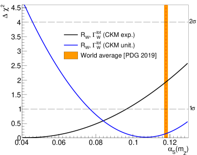
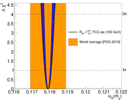
Figure 22: $\Delta\chi^{2}$ fit profiles of the $\alpha_{S}(m^{2}_{\mathrm{Z}})$ determined from the combined N³LO analysis of the total W width and $R_{\mathcal{W}}$ ratio, compared to the 2019 $\alpha_{S}(m^{2}_{\mathrm{Z}})$ world average (vertical orange band). Left: Extraction with the present W data assuming (blue curve) or not (black curve) CKM unitarity. Right: Extraction expected at the FCC-ee, with the total (experimental, parametric, and theoretical in quadrature) uncertainties (outer parabola) and with the experimental uncertainties alone (inner parabola).

b $\alpha_{S}(m^{2}_{\mathrm{Z}})$ from Z boson decays

For the Z boson case, we incorporate into the gfitter v2.2 code Haller:2018nnx all parametrizations of the partial and total Z widths, including the full two-loop ${\cal O}(\alpha^{2})$ electroweak terms given in Ref. Dubovyk:2018rlg , plus the leading fermionic three-loop ${\cal O}(\alpha^{3})$ EW corrections of Ref. Chen:2020xzx . These 2-loop (leading fermionic 3-loop) EW corrections increase the theoretical predictions for $\Gamma_{\mathrm{Z}}^{\mathrm{tot}}$ by $+0.83$ MeV ($+0.33$ MeV), $R_{\mathrm{Z}}$ by $+0.0186$ ($-0.0037$), and $\sigma_{\mathrm{Z}}^{\mathrm{had}}$ by $+1$ pb. The theoretical errors from missing higher-order ${\cal O}(\alpha^{3})$ EW, ${\cal O}(\alpha^{5})$ QCD, and ${\cal O}(\alpha\alpha_{S}^{2},\,\alpha\alpha_{S}^{3},\,\alpha^{2}\alpha_{S})$ mixed corrections estimated in Refs. Dubovyk:2018rlg ; Chen:2020xzx are of relative size of $\sim$1.5$\cdot 10^{-4}$ for $\Gamma_{\mathrm{Z}}^{\mathrm{tot}}$ and $\sigma_{\mathrm{Z}}^{\mathrm{had}}$, and $\sim$2.5$\cdot 10^{-4}$ for $\mathrm{R}_{\mathrm{Z}}$, i.e. they are about a factor of two better than the corresponding theoretical calculations for the W boson pseudoobservables, as expected since the EW accuracy of the latter is only ${\cal O}(\alpha)$ today.

On the experimental data, new studies Voutsinas:2019hwu ; Janot:2019oyi have updated the LEP luminosity corrections at and off the resonance peak that modify the PDG results for the Z boson pseudoobservables $\Gamma_{\mathrm{Z}}^{\mathrm{tot}}$, and $\sigma_{\mathrm{Z}}^{\mathrm{had}}$. The change in $\Gamma_{\mathrm{Z}}^{\mathrm{tot}}$ is of $+0.012\%$. The impact on $\sigma_{\mathrm{Z}}^{\mathrm{had}}$ is the largest of all pseudoobservables, with a $0.144\%$ reduction of the hadronic cross section at the Z peak that brings the data very close to the theoretical prediction. The central $\rm R_{\mathrm{Z}}$ ratios have not changed, but an extra precision digit is added now. The experimental uncertainties today ($\sim$0.1%) are about a factor of four larger than their theoretical or parametric counterparts ($\sim$0.025%). Matching the uncertainties of the current theory state-of-the-art calls for higher precision measurements in ${\rm e^{+}e^{-}}$ collisions at the Z pole with, at least, 20 times larger data samples than those collected at LEP.

The extraction of $\alpha_{S}(m^{2}_{\mathrm{Z}})$ is carried out with 1-D scans of this variable as a free parameter using single and combined observables with our updated version of gfitter 2.2. The results from these fits are listed in Table 9, and the corresponding $\Delta\chi^{2}$ profiles are plotted in Fig. 23. The solid lines represent the results of the present improved calculations and data, whereas the dashed lines are those obtained with gfitter in 2018 Haller:2018nnx . All new QCD couplings are clustered around $\alpha_{S}(m^{2}_{\mathrm{Z}})=0.1200$, whereas previously the extraction from $\sigma_{\mathrm{Z}}^{\mathrm{had}}$ was about 2$\sigma$ lower (and also had larger uncertainties) than the average of the three, and that from $\mathrm{R}_{\mathrm{Z}}$ was 1$\sigma$ above it. Among $\alpha_{S}(m^{2}_{\mathrm{Z}})$ extractions, the most precise is that from $\mathrm{R}_{\mathrm{Z}}$ (3.4% uncertainty), followed by the ones from $\Gamma_{\mathrm{Z}}^{\mathrm{tot}}$ (3.9% uncertainty) and $\sigma_{\mathrm{Z}}^{\mathrm{had}}$ (5.6% uncertainty). The precision did not change appreciably compared to the previous $\Gamma_{\mathrm{Z}}^{\mathrm{tot}}$ and $\mathrm{R}_{\mathrm{Z}}$ results, but the extraction from the hadronic Z cross section has been improved by about 20% thanks mostly to the updated LEP data. When combining various Z observables, their associated correlation matrix is used in the fit. Table 9 lists all results with their propagated uncertainties broken down into experimental, parametric, and theoretical sources. Our final values, $\alpha_{S}(m^{2}_{\mathrm{Z}})=0.1203\pm 0.0028$ from the combined Z boson data, and $\alpha_{S}(m^{2}_{\mathrm{Z}})=0.1202\pm 0.0028$ from the full SM fit, and the PDG electroweak fit result ($\alpha_{S}(m^{2}_{\mathrm{Z}})=0.1203\pm 0.0028$) Zyla:2020zbs are all virtually identical now.

Table 9: Values of $\alpha_{S}(m^{2}_{\mathrm{Z}})$ determined at N³LO accuracy from $\Gamma_{\mathrm{Z}}^{\mathrm{tot}}$, $R_{\mathrm{Z}}$, and $\sigma_{\mathrm{Z}}^{\mathrm{had}}$ individually, combined, as well as from a global SM fit, with propagated experimental, parametric, and theoretical uncertainties broken down. The last two rows list the expected values at the FCC-ee from all Z pseudoobservables combined and from the corresponding SM fit.

Observable	$\alpha_{S}(m^{2}_{\mathrm{Z}})$	uncertainties
		exp.	param.	theor.
$\Gamma_{\mathrm{Z}}^{\mathrm{tot}}$	$0.1192\pm 0.0047$	$\pm 0.0046$	$\pm 0.0005$	$\pm 0.0008$
$R_{\mathrm{Z}}$	$0.1207\pm 0.0041$	$\pm 0.0041$	$\pm 0.0001$	$\pm 0.0009$
$\sigma_{\mathrm{Z}}^{\mathrm{had}}$	$0.1206\pm 0.0068$	$\pm 0.0067$	$\pm 0.0004$	$\pm 0.0012$
All above combined	$0.1203\pm 0.0029$	$\pm 0.0029$	$\pm 0.0002$	$\pm 0.0008$
Global SM fit	$0.1202\pm 0.0028$	$\pm 0.0028$	$\pm 0.0002$	$\pm 0.0008$
All combined (FCC-ee)	$0.12030\pm 0.00026$	$\pm 0.00013$	$\pm 0.00005$	$\pm 0.00022$
Global SM fit (FCC-ee)	$0.12020\pm 0.00026$	$\pm 0.00013$	$\pm 0.00005$	$\pm 0.00022$

At the FCC-ee, combining the $3\cdot 10^{12}$ Z bosons decaying hadronically at the Z pole, and the $\mathcal{O}$(tens of keV)-accurate $\sqrt{s}$ calibration obtained using resonant depolarization Blondel:2021zix , will provide measurements with unparalleled precision. The statistical uncertainties in the Z mass and width, today of $\pm$1.2 MeV and $\pm$2 MeV (dominated by the LEP beam energy calibration), will be reduced to below $\pm$4 keV and $\pm$7 keV respectively. Similarly, the statistical uncertainty in $\mathrm{R}_{\mathrm{Z}}^{\mathrm{exp}}$ will be negligible and the measurement in the Z $\to\mu^{+}\mu^{-}$ final state alone, yielding an experimental precision of 0.001 from the knowledge of the detector acceptance, will suffice to reach an absolute (relative) uncertainty of 0.001 ($5\cdot 10^{-5}$) on the ratio of the hadronic-to-leptonic partial Z widths. Thus, accounting for the dominant experimental systematic uncertainties at the FCC-ee, we expect: $\delta m_{\mathrm{Z}}$ = 0.025–0.1 MeV, $\delta\Gamma_{\mathrm{Z}}^{\mathrm{tot}}=0.1$ MeV, $\delta\sigma_{\mathrm{Z}}^{\mathrm{had}}=4.0$ pb, and $\delta\mathrm{R}_{\mathrm{Z}}=10^{-3}$ relative uncertainties FCC:2018evy . In addition, the QED coupling at the Z peak will be measured with a precision of $\delta\alpha=3\cdot 10^{-5}$ Janot:2015gjr , thereby also reducing the corresponding propagated parametric uncertainties. Implementing the latter uncertainties into our updated gfitter setup, namely taking $\Gamma_{\mathrm{Z}}^{\mathrm{tot}}=2495.2\pm 0.1$ MeV, $\sigma_{\mathrm{Z}}^{\mathrm{had}}=41\,494\pm 4$ pb, and $\mathrm{R}_{\mathrm{Z}}=20.7500\pm 0.0010$, as well as $m_{\mathrm{Z}}=91.18760\pm 0.00001$ GeV, and $\delta\alpha_{\mathrm{had}}^{(5)}(m_{\mathrm{Z}})=0.0275300\pm 0.0000009$, we derive the results listed in the last two rows of Table 9 where, the central $\alpha_{S}(m^{2}_{\mathrm{Z}})$ value is arbitrarily set at the current SM global fit extraction. The final uncertainties in the QCD coupling constant are reduced to the $\sim$0.1% level, namely about three times smaller than the propagated theoretical uncertainties today. Theoretical developments in the years to come should further bring down the latter by a factor of four Proceedings:2019vxr . A final QCD coupling constant extraction at the FCC-ee with a 2-permil total uncertainty is thereby reachable: $\alpha_{S}(m^{2}_{\mathrm{Z}})=0.12030\pm 0.00013_{\mathrm{exp}}\pm 0.00005_{\mathrm{par}}\pm 0.00022_{\mathrm{th}}$ (Table 9). Figure 23 (right) shows the $\Delta\chi^{2}$ parabola for the $\alpha_{S}(m^{2}_{\mathrm{Z}})$ extraction from the Z boson data (or from the SM fit that is almost identical) expected at the FCC-ee (with the central value arbitrarily set to its present result), compared to the same extraction today (blue parabola) and to the 2018 world average (orange band). The large improvement, by more than a factor of ten, in the FCC-ee extraction of $\alpha_{S}(m^{2}_{\mathrm{Z}})$ from the Z boson data (and its comparison to the similar extraction from the W boson, Fig. 22 right) will enable searches for small deviations from the SM predictions that could signal the presence of new physics contributions.

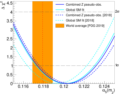
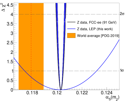
Figure 23: $\Delta\chi^{2}$ fit profiles of $\alpha_{S}(m^{2}_{\mathrm{Z}})$ determined from the combined Z boson pseudoobservables analysis and/or the global SM fit compared to the 2019 world average (orange band). Left: Current results (solid lines) compared to the previous 2018 fit (dashed lines). Right: Extraction expected at the FCC-ee –with central value (arbitrarily) set to $\alpha_{S}(m^{2}_{\mathrm{Z}})=0.12030$ and total (experimental, parametric, and theoretical in quadrature) uncertainties (outer parabola) and experimental uncertainties alone (inner parabola)– compared to the present one from the combined Z data (blue line).

VI $\alpha_{S}(m^{2}_{\mathrm{Z}})$ from hadronic final-states in ${\rm e^{+}e^{-}}$ collisions

1 Hadronic vacuum polarization function, R-ratio, and the strong coupling

The process of electron-positron annihilation into hadrons plays a distinctive role in elementary particle physics. This is primarily caused by a remarkable fact that its theoretical description requires no phenomenological models of hadronization, which forms the experimentally detected final-state particles. In turn, this feature makes it possible to extract the key parameters of the theory from pertinent experimental data in the model-independent way, thereby constituting one of the cleanest methods of their determination.

In the theoretical studies of ${\rm e^{+}e^{-}}$ annihilation into hadrons one needs to operate with the physical observable, which depends on the timelike kinematic variable (namely, the center-of-mass energy squared $s=q^{2}>0$), whereas such basic tools as the perturbative technique and the renormalization group method are directly applicable only to the quantities, which depend on the spacelike kinematic variable $Q^{2}=-q^{2}>0$. The proper description of the strong interactions in the timelike domain substantially relies on the corresponding dispersion relations, which provide the physically consistent way to interrelate the “timelike” experimentally measurable observables (such as the $R$-ratio of ${\rm e^{+}e^{-}}$ annihilation into hadrons) with the “spacelike” theoretically computable quantities (such as the hadronic vacuum polarization function and the Adler function), see, e.g., Ref. Nesterenko:2016pmx and references therein for the details.

The hadronic vacuum polarization function $\Pi(q^{2})$ is defined as the scalar part of the hadronic vacuum polarization tensor

$$\Pi_{\mu\nu}(q^{2})=i\!\int\!d^{4}x\,e^{iqx}\bigl{\langle}0\bigl{|}\,T\!\left\{J_{\mu}(x)\,J_{\nu}(0)\right\}\bigr{|}0\bigr{\rangle}=\frac{i}{12\pi^{2}}(q_{\mu}q_{\nu}-g_{\mu\nu}q^{2})\Pi(q^{2}),\qquad q^{2}<0.$$ (116)

The physical kinematic restrictions on the process on hand define the location of the cut of the function $\Pi(q^{2})$ in the complex $q^{2}$-plane, that, in turn, enables one to write down the corresponding dispersion relation. In particular, as discussed in, e.g., Ref. Feynman:1973xc , for the processes involving final state hadrons the function $\Pi(q^{2})$ (116) possesses the only cut along the positive semiaxis of real $q^{2}$ starting at the hadronic production threshold $q^{2}\geq 4m_{\pi}^{2}$, that implies

$$\Pi(q^{2})-\Pi(q_{0}^{2})=(q^{2}-q_{0}^{2})\!\int\limits_{4m_{\pi}^{2}}^{\infty}\!\frac{R(\sigma)}{(\sigma-q^{2})(\sigma-q_{0}^{2})}\,d\sigma,$$ (117)

where

$$R(s)=\frac{1}{2\pi i}\lim_{\varepsilon\to 0_{+}}\Bigl{[}\Pi(s+i\varepsilon)-\Pi(s-i\varepsilon)\Bigr{]}\!=\frac{1}{\pi}\,{\rm Im}\!\lim_{\varepsilon\to 0_{+}}\!\Pi(s+i\varepsilon).$$ (118)

The function $R(s)$ (118) is commonly identified with the $R$-ratio of ${\rm e^{+}e^{-}}$ annihilation into hadrons $R(s)=\sigma(e^{+}e^{-}\!\to\text{hadrons};s)/\sigma(e^{+}e^{-}\!\to\mu^{+}\mu^{-};s)$. For the practical purposes it proves to be convenient to deal with the Adler function Adler:1974gd

$$D(Q^{2})=-\frac{d\,\Pi(-Q^{2})}{d\ln Q^{2}},\qquad Q^{2}=-q^{2}>0$$ (119)

and the other relations between the functions $\Pi(q^{2})$, $D(Q^{2})$, and $R(s)$ can be directly obtained from Eqs. (117)–(119). Note that the massless limit $m_{\pi}=0$ is assumed in what follows.

In the framework of perturbation theory the Adler function (119) acquires the form of power series in the function $a^{(\ell)}_{{\rm s}}(Q^{2})=\alpha_{S}^{(\ell)}(Q^{2})\,\beta_{0}/(4\pi)$ [with $\alpha_{S}^{(\ell)}(Q^{2})$ being the strong coupling], namely

$$D^{(\ell)}(Q^{2})=1+d^{(\ell)}(Q^{2}),\qquad d^{(\ell)}(Q^{2})=\!\sum_{j=1}^{\ell}d_{j}\!\left[a^{(\ell)}_{{\rm s}}(Q^{2})\right]^{j}\!.$$ (120)

In this equation, $\ell$ specifies the loop level, $d_{1}=4/\beta_{0}$, $\beta_{0}=11-2n_{f}/3$, $n_{f}$ is the number of active flavors, and the common prefactor $N_{\text{c}}\sum_{f=1}^{n_{f}}Q_{f}^{2}$ is omitted throughout, where $N_{\text{c}}=3$ denotes the number of colors and $Q_{f}$ stands for the electric charge of $f$-th quark. The function $a^{(\ell)}_{{\rm s}}(Q^{2})$ entering Eq. (120) can be represented as the double sum

$$a^{(\ell)}_{{\rm s}}(Q^{2})=\sum_{n=1}^{\ell}\sum_{m=0}^{n-1}b^{m}_{n}\,\frac{\ln^{m}(\ln z)}{\ln^{n}z},\qquad z=\frac{Q^{2}}{\Lambda^{2}},$$ (121)

where $\Lambda$ is the QCD scale parameter and $b^{m}_{n}$ (the integer superscript $m$ is not to be confused with respective power) stands for the combination of the $\beta$ function perturbative expansion coefficients (in particular, $b^{0}_{1}=1$, $b^{0}_{2}=0$, $b^{1}_{2}=-\beta_{1}/\beta_{0}^{2}$, see, e.g., Appendix A of Ref. Nesterenko:2016pmx ). The Adler function perturbative expansion coefficients $d_{j}$ (120) were calculated up to the fourth order in the strong coupling ($1\leq j\leq 4$), see Refs. Baikov:2008jh ; Baikov:2010je ; Baikov:2012zn and references therein, whereas the $\beta$ function perturbative expansion coefficients $\beta_{j}$ appearing in Eq. (121) are available up to the five-loop level ($0\leq j\leq 4$), see Refs. Baikov:2016tgj ; Herzog:2017ohr ; Luthe:2017ttg and references therein.

The explicit expression for the $R$-ratio of ${\rm e^{+}e^{-}}$ annihilation into hadrons, which properly accounts for all the effects due to continuation of the spacelike perturbative results into the timelike domain, is obtained at an arbitrary loop level Nesterenko:2017wpb ; Nesterenko:2019rag

$$R^{(\ell)}(s)=1+r^{(\ell)}(s),\qquad r^{(\ell)}(s)=\sum\limits_{j=1}^{\ell}d_{j}\,A^{(\ell)}_{{\rm TL},j}(s).$$ (122)

In this equation $d_{j}$ stand for the Adler function perturbative expansion coefficients (120),

$$A^{(\ell)}_{{\rm TL},j}(s)=\sum_{n_{1}=1}^{\ell}\ldots\sum_{n_{j}=1}^{\ell}\sum_{m_{1}=0}^{n_{1}-1}\ldots\sum_{m_{j}=0}^{n_{j}-1}\Biggl{(}\prod_{i=1}^{j}b^{m_{i}}_{n_{i}}\Biggr{)}\mbox{\tiny$\,$}T\mbox{\tiny$\!$}\Biggl{(}\!s,\sum_{i=1}^{j}n_{i},\sum_{i=1}^{j}m_{i}\!\Biggr{)}$$ (123)

denotes the $\ell$-loop $j$-th order “timelike” effective expansion function (that constitutes the corresponding continuation of the $j$-th power of $\ell$-loop function $\bigl{[}a^{(\ell)}_{{\rm s}}(Q^{2})\bigr{]}^{j}$ from spacelike into the timelike domain), the coefficients $b^{m}_{n}$ are specified in Eq. (121),

$$T(s,n,m)=\begin{cases}\displaystyle-V_{0}^{1}(s),&\text{if $\,n=1\,$ and $\,m=0$},\\[7.11317pt] \displaystyle\sum_{k=0}^{m}\frac{m!}{k!}(n-1)^{k-m-1}\,V_{n-1}^{k}(s),\quad&\text{if $\,n\geq 2$},\end{cases}$$ (124)

$$V_{n}^{m}(s)=\begin{cases}0,\quad&\text{if $\,n=0\,$ and $\,m=0$},\\[3.55658pt] v_{0}^{m}(s),\quad&\text{if $\,n=0\,$ and $\,m\geq 1$},\\[3.55658pt] v_{n}^{0}(s),&\text{if $\,n\geq 1\,$ and $\,m=0$},\\[3.55658pt] v_{n}^{0}(s)u_{0}^{m}(s)+u_{n}^{0}(s)v_{0}^{m}(s),\quad&\text{if $\,n\geq 1\,$ and $\,m\geq 1$},\end{cases}$$ (125)

$$v_{0}^{m}(s) =\!\sum\limits_{k=0}^{K(m)}\!\binom{m}{2k+1}(-1)^{k+1}\pi^{2k}\Bigl{[}L_{1}(y)\Bigr{]}^{m-2k-1}\,\Bigl{[}L_{2}(y)\Bigr{]}^{2k+1},$$ (126)

$$v_{n}^{0}(s) =\frac{1}{(y^{2}+\pi^{2})^{n}}\sum_{k=0}^{K(n)}\!\binom{n}{2k+1}(-1)^{k}\pi^{2k}y^{n-2k-1},$$ (127)

$$u_{0}^{m}(s) =\!\sum\limits_{k=0}^{K(m+1)}\!\binom{m}{2k}(-1)^{k}\pi^{2k}\Bigl{[}L_{1}(y)\Bigr{]}^{m-2k}\,\Bigl{[}L_{2}(y)\Bigr{]}^{2k},$$ (128)

$$u_{n}^{0}(s) =\frac{1}{(y^{2}+\pi^{2})^{n}}\sum_{k=0}^{K(n+1)}\!\binom{n}{2k}(-1)^{k}\pi^{2k}y^{n-2k},$$ (129)

$$L_{1}(y)=\ln\!\sqrt{y^{2}+\pi^{2}},\quad L_{2}(y)=\frac{1}{2}-\frac{1}{\pi}\arctan\biggl{(}\frac{y}{\pi}\biggr{)},\quad\binom{n}{m}=\frac{n!}{m!\,(n-m)!},\quad K(n)=\frac{n-2}{2}+\frac{n\;\mbox{mod}\;2}{2},$$ (130)

$(n\;\mbox{mod}\;m)$ denotes the remainder on division of $n$ by $m$, it is assumed that $\arctan(x)$ is a monotone nondecreasing function of its argument [namely, $-\pi/2\leq\arctan(x)\leq\pi/2$ for $-\infty<x<\infty$], and $y=\ln(s/\Lambda^{2})$, see Refs. Nesterenko:2017wpb ; Nesterenko:2019rag for the details.

At the same time, the commonly employed expression for the $R$-ratio of ${\rm e^{+}e^{-}}$ annihilation into hadrons reads (see, e.g., Ref. Zyla:2020zbs )

$$R^{(\ell)}_{{\rm appr}}(s)=1+\sum_{j=1}^{\ell}r_{j}\Bigl{[}a^{(\ell)}_{{\rm s}}(|s|)\Bigr{]}^{j},\qquad r_{j}=d_{j}-\delta_{j},$$ (131)

where $d_{j}$ stand for the Adler function perturbative expansion coefficients (120) and $\delta_{j}$ embody the contributions of the so-called $\pi^{2}$-terms, which play a significant role in the studies of the process on hand (see, e.g., Ref. Bjorken:1989xw ). The explicit expression for the coefficients $\delta_{j}$ is obtained at an arbitrary loop level Nesterenko:2020nol , specifically ($\delta_{1}=\delta_{2}=0$)

$$\delta_{j}= -\sum_{k=1}^{K(j)}\frac{(-2\pi^{2})^{k}}{(2k+1)!}\sum_{i_{1}=2(k-1)+1}^{j-2}\underbrace{\sum_{i_{2}=2(k-2)+1}^{i_{1}-2}\ldots\sum_{i_{n}=2(k-n)+1}^{i_{n-1}-2}\ldots\sum_{i_{k}=1}^{i_{k-1}-2}}_{\mbox{{\small$(k-1)$~{}sums}}}(j+i_{1})i_{1}\times$$

$$\times\underbrace{(i_{1}+i_{2})i_{2}\times\ldots\times(i_{n-1}+i_{n})i_{n}\times\ldots\times(i_{k-1}+i_{k})i_{k}}_{\mbox{{\small$(k-1)$~{}products}}}\times$$

$$\times\mathfrak{B}_{j-i_{1}-2}\underbrace{\mathfrak{B}_{i_{1}-i_{2}-2}\ldots\mathfrak{B}_{i_{n-1}-i_{n}-2}\ldots\mathfrak{B}_{i_{k-1}-i_{k}-2}}_{\mbox{{\small$(k-1)$~{}terms}}}d_{i_{k}},\quad\mathfrak{B}_{n}=\frac{1}{4}\sum_{i=0}^{n}B_{i}\,B_{n-i},\quad B_{i}=\frac{\beta_{i}}{\beta_{0}^{i+1}},\quad j\geq 3.$$ (132)

It is necessary to emphasize that, as argued in, e.g., Refs. Moorhouse:1976qq ; Pennington:1981cw ; Pennington:1983rz ; Pivovarov:1991bi , the effects due to continuation of the spacelike perturbative results into the timelike domain are only partially accounted for in Eq. (131) by the coefficients $\delta_{j}$, whereas the ignorance (complete or partial) of such effects may yield misleading results. In particular, it was shown Nesterenko:2017wpb ; Nesterenko:2019rag ; Nesterenko:2020nol that the approximation $R_{{\rm appr}}(s)$ (131) factually constitutes the truncated re-expansion of the proper expression $R(s)$ (122) at high energies and the validity range of such re-expansion is strictly limited to $\sqrt{s}>\Lambda\exp(\pi/2)\simeq 4.81\,\Lambda$. Moreover, the contribution of a given order to the proper expression for the $R$-ratio (122) appears to be redistributed over the higher-order terms in its approximate form (131), thereby substantially amplifying them. In turn, this makes the loop convergence of a commonly employed approximation of the $R$-ratio (131) much worse than that of its proper form (122) and increases the resulting theoretical uncertainty of the strong coupling and the QCD scale parameter associated with the higher-loop perturbative corrections disregarded in Eq. (131). Basically, the aforementioned truncation of the re-expansion of the proper expression for the $R$-ratio (122) neglects all the higher-order $\pi^{2}$-terms in Eq. (131), though the latter may not necessarily be negligible. Specifically, it was shown that the higher-order $\pi^{2}$-terms omitted in a commonly employed approximation $R_{{\rm appr}}(s)$ (131) can produce a considerable effect on the determination of the strong coupling and the QCD scale parameter from the experimental data on the $R$-ratio, see Refs. Nesterenko:2017wpb ; Nesterenko:2019rag ; Nesterenko:2020nol for the details.

2 $\alpha_{S}(m^{2}_{\mathrm{Z}})$ from soft parton fragmentation functions

We summarize a derivation of the QCD coupling $\alpha_{S}$ from the energy evolution of the moments of the parton-to-hadron fragmentation functions (FFs) at low hadron Feynman momentum fraction $z$. In Refs. Perez-Ramos:2013eba ; dEnterria:2014lmi ; dEnterria:2014xmb ; Perez-Ramos:2014pua ; dEnterria:2015ljg , the energy evolution of the moments of the parton-to-hadron FFs were computed up to approximate next-next-to-leading-order (NNLO^⋆) fixed-order including next-to-next-to-leading-log (NNLL) resummation corrections. A fit to the corresponding experimental jet data from ${\rm e^{+}e^{-}}$ and deep-inelastic e${}^{\pm},\nu$-p collisions, to the NNLO^∗+NNLL predictions yields $\alpha_{S}(m^{2}_{\mathrm{Z}})=0.1205\pm 0.0010\,\mathrm{(exp)}\pm 0.0022$ (th), in good agreement with the current $\alpha_{S}$ world average. Forthcoming prospects based on full-NNLO calculations are discussed.

The conversion of a quark and gluon (collectively called partons) into a final jet of hadrons is driven by soft and collinear gluon bremsstrahlung Dokshitzer:1982ia followed by the final transformation into hadrons of the last partons produced in the QCD shower at non-perturbative scales approaching $\Lambda_{\mathrm{QCD}}$. The distribution of hadrons inside a jet is described by its fragmentation function, $D_{\rm a\to h}(z,Q)$, that encodes the probability that an initial parton $a$ eventually fragments into a hadron $h$ carrying a fraction $z=p_{\rm hadron}/p_{\rm parton}$ of the parent parton’s momentum. Starting with a parton at a given $\delta$-function energy $Q$, its evolution to any other lower energy scale $Q^{\prime}$ is driven by a branching process of parton radiation and splitting, $a\to b\,c$, that can be perturbatively computed. At large $z\gtrsim 0.1$ one uses the DGLAP evolution equations Gribov:1972ri ; Altarelli:1977zs ; Dokshitzer:1977sg , whereas the Modified Leading Logarithmic Approximation (MLLA) Dokshitzer:1991ej , resumming soft and collinear logs along with hard and collinear logs, provides an appropriate theoretical framework at small $z$. In this latter approach, one writes the FF as a function of the log of the inverse of $z$, i.e. $\xi=\ln(1/z)$, in order to describe the region of low hadron momenta that dominates the jet fragments. Due to colour coherence and interference in gluon radiation (angular ordering), not the softest partons but those with intermediate energies multiply most effectively in QCD cascades, leading to a final FF with a typical “hump-backed plateau” (HBP) shape as a function of $\xi$ (Fig. 24, left). Such a shape can be perfectly reproduced by a distorted Gaussian (DG, Fong:1990nt ) in terms of the hadron multiplicity ${\cal N}$ (giving the integral, and thereby the normalization, of the DG), the mean peak position $\bar{\xi}$, the dispersion $\sigma$, the skewness $s$, and kurtosis $k$ of the distribution.

In Refs. dEnterria:2014lmi , we described a new approach that solves the set of integro-differential equations for the FF evolution combining both DGLAP and MLLA corrections. This is done by expressing the Mellin-transformed hadron distribution in terms of the anomalous dimension $\gamma$: $D\simeq C(\alpha_{S}(t))\exp\left[\int^{t}\gamma(\alpha_{S}(t^{\prime}))dt\right]$ where $t=\ln Q$ is the “time” evolution variable in QCD parton showers. The analysis leads to a series in half powers of $\alpha_{S}$: $\gamma\sim{\cal O}(\alpha_{S}^{{}^{1/2}})+{\cal O}(\alpha_{S})+{\cal O}(\alpha_{S}^{{}^{3/2}})+{\cal O}(\alpha_{S}^{{}^{2}})+{\cal O}(\alpha_{S}^{{}^{5/2}})+\cdots$, where integer powers of $\alpha_{S}$ correspond to fixed-order corrections, and half-integer terms can be identified with increasingly accurate resummations of soft and collinear logarithms. The full set of NLO ${\cal O}(\alpha_{S}^{2})$ terms for the anomalous dimension, including the one-loop splitting functions $P_{ac}^{(1)}$ and the two-loop running of $\alpha_{S}$, plus a fraction of the ${\cal O}(\alpha_{S}^{{}^{5/2}})$ terms, coming from the NNLO expression of $\alpha_{S}$ have been computed DdERPR . Upon inverse-Mellin transformation, one can derive the analytical expressions for the energy evolution of the FF, and its associated moments, as a function of $Y=\ln(E/\Lambda_{\mathrm{QCD}})$, for an initial parton energy $E$, down to a shower cutoff scale $Q_{0}>\Lambda_{\mathrm{QCD}}$ for $N_{f}=3,4,5$ quark flavors. By introducing $\lambda=\ln(Q_{0}/\Lambda_{\mathrm{QCD}})$, the resulting formulas for the energy evolution of the moments depend on $\Lambda_{\mathrm{QCD}}$ as a single free parameter. Simpler expressions can be further obtained for $Q_{0}\to\Lambda_{\mathrm{QCD}}$ (limiting spectrum) motivated by the “local parton hadron duality” hypothesis for inclusive-enough observables. Thus, by fitting to the distorted Gaussian, the measured HBP at various energies, one can determine $\alpha_{S}$ from the corresponding jet energy-dependence of the FF moments ${\cal N}$, $\bar{\xi}$, $\sigma$, $s$, and $k$.

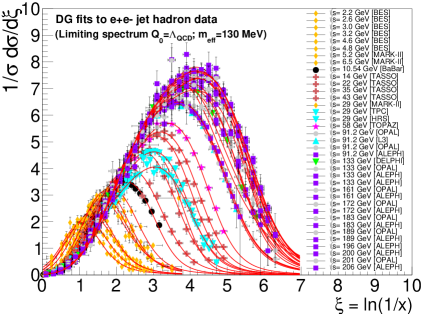
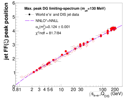
Figure 24: Left: HBP charged-hadron distributions in jets as a function of $\xi=\ln(1/z)$ measured in ${\rm e^{+}e^{-}}$ at $\sqrt{s}\approx$ 2–200 GeV, fitted to a DG distribution. Right: Energy evolution of the peak position of the DG measured in ${\rm e^{+}e^{-}}$ and DIS data fitted to the NNLO^⋆+NNLL predictions.

In the phenomenological analysis, we first start by fitting to the DG all existing jet FF data measured in ${\rm e^{+}e^{-}}$ and e${}^{\pm},\nu$-p collisions over $\sqrt{s}\approx$ 1–200 GeV, and thereby derive the corresponding FF moments at each jet energy Perez-Ramos:2019zxf . The overall normalization of the HBP spectrum (${\cal K}_{\rm ch}$), which determines the average charged-hadron multiplicity of the jet (i.e. the zeroth moment of the FF), is an extra free parameter in the DG fit which, nonetheless, plays no role in the finally derived $\Lambda_{\mathrm{QCD}}$ value since the latter is solely dependent on the relative evolution of the multiplicity, and not on its absolute value at any given jet energy. The impact of finite hadron-mass effects in the DG fit are taken into account through a rescaling of the theoretical (massless) parton momenta with an effective mass $m{{}_{\mathrm{eff}}}\approx m_{\pi}$. Varying such effective mass from zero to a few hundred MeV, results in small propagated uncertainties into the final extracted $\Lambda_{\mathrm{QCD}}$ (and associated $\alpha_{S}(m^{2}_{\mathrm{Z}})$) value, as discussed in Refs. dEnterria:2014lmi .

Once the energy evolution of all FF moments has been obtained from the individual experimental measurements, one can perform a combined fit of them as a function of the original parton energy. In the case of ${\rm e^{+}e^{-}}$ collisions, the latter corresponds to half the centre-of-mass energy $\sqrt{s}/2$ whereas, for DIS, the invariant four-momentum transfer $Q_{{}_{\rm DIS}}$ is used. The experimental and theoretical evolutions of the hadron multiplicity and FF peak position as a function of jet energy are shown in Perez-Ramos:2019zxf . The hadron multiplicities measured in DIS jets appear somewhat smaller (especially at high energy) than those from ${\rm e^{+}e^{-}}$ collisions, due to limitations in the FF measurement only in half (current Breit) e^±-p hemisphere and/or in the determination of the relevant $Q$ scale dEnterria:2014lmi . The NNLO^⋆+NNLL limiting-spectrum ($\lambda=0$) predictions for $N_{f}=5$ active quark flavours (the moments of the lowest-$\sqrt{s}$ data have a few-percent correction applied in order to account for the slightly different ($N_{f}=3,4$) evolutions below the charm and bottom production thresholds), leaving $\Lambda_{\mathrm{QCD}}$ as a free parameter, reproduce very well the data. Fit results for the rest of the FF moments can be found in dEnterria:2014lmi . Figure 24 (right) shows the result of the peak position fit. Among FF moments, the peak position $\xi_{\rm max}$ appears as the most “robust” for the determination of $\Lambda_{\mathrm{QCD}}$, being relatively insensitive to most of the uncertainties associated with the extraction method (DG fits, energy evolution fits, finite-mass corrections, …) as well as to higher-order corrections Perez-Ramos:2019zxf . Finally, the energy evolution of all or a fraction of HBP moments can be simultaneously fitted to the corresponding theoretical predictions in the limiting-spectrum case with just $\Lambda_{\mathrm{QCD}}$ as single free parameter.

The QCD coupling obtained from the combined fit of the multiplicity and peak position is $\alpha_{S}(m^{2}_{\mathrm{Z}})=0.1205\pm 0.0010\,(\mathrm{exp})\,\pm 0.0022\,(\mathrm{theo})$, where the first uncertainty includes all experimentally-related sources discussed in Refs. dEnterria:2014lmi , and the second one is a theoretical scale uncertainty derived at NLO by stopping the parton evolution of the FFs at $Q_{{}_{0}}=1$ GeV rather than at the limiting spectrum value $Q_{{}_{0}}=\Lambda_{\mathrm{QCD}}$. Our extracted $\alpha_{S}(m^{2}_{\mathrm{Z}})$ value is consistent with all other NNLO results from the latest PDG compilation Zyla:2020zbs , as well as with other determinations with a lower degree of theoretical accuracy dEnterria:2018cye . The precision of our result ($\pm 2\%$) is competitive with the other extractions, with a totally different set of experimental and theoretical uncertainties.

Outlook:

Given the robustness of the observables chosen, energy evolution of FF moments, the purely experimental uncertainties of our $\alpha_{S}(m^{2}_{\mathrm{Z}})$ extraction are small, $\sim$0.8%, and will be eventually negligible with the large jet data samples, orders of magnitude larger than those at LEP, expected to be collected at future ${\rm e^{+}e^{-}}$ machines Proceedings:2017ocd ; FCC:2018evy . Thus, the main source of imprecision is of theoretical origin. The main theoretical challenges of the approach presented here are to match the MLLA anomalous dimension to the $\overline{\mathrm{MS}}$ anomalous dimension and to reach full-NNLO pQCD accuracy. It is known that the MLLA anomalous dimension obtained within the massive gluon (MG) regularization scheme Mueller:1982cq turns out to be inconsistent with the expected N⁴LL+NNLO result in the $\overline{\mathrm{MS}}$ scheme. For instance, the inconsistency between NNLO DLs terms to the anomalous dimension calculated in Mueller:1982cq and those calculated in Mitov:2006ic can be explained from the use of different regularization and factorization schemes Albino:2011si . More recently, it has been noticed that the main difference is entirely due to running coupling effects being truncated in a quite severe way Neill:2020tzl . In addition, in order to extract a coupling constant with NNLO fixed-order accuracy from the moments of the FFs, the diagonalisation of the matrix elements (i.e. the splitting functions) beyond the ${\cal O}(\alpha_{S}^{5/2})$ order is a crucial step forwards. The diagonalisation method to be adopted was considered a major technical challenge since the splitting functions do not commute beyond leading order. However, it becomes now possible thanks to the recent work by Kotikov and Teryaev Kotikov:2020ukv . To conclude, the implementation of the approach used in Kotikov:2020ukv and the change from the MG regularization scheme to the $\overline{\mathrm{MS}}$ scheme may make it possible to complete the present programme on the full-NNLO extraction of $\alpha_{S}(m^{2}_{\mathrm{Z}})$ from the moments of FFs within the $\overline{\mathrm{MS}}$ factorization scheme.

3 Power corrections to event-shape distributions and impact on $\alpha_{S}$ extractions

In this brief note we discuss some recent developments on the fits of $\alpha_{S}$ from event-shape distributions at lepton colliders. These determinations rely on the fact that event shape variables that vanish in the two-jet limit are directly sensitive to the QCD $q\bar{q}g$ vertex, and thus arguably offer one of the simplest frameworks to extract the strong coupling constant. The present status of these measurements as reported in the Particle Data Group (PDG) Zyla:2020zbs ; ParticleDataGroup:2018ovx is not very satisfactory. In particular, determinations in which nonperturbative corrections are estimated via analytic models tend to give values for the strong coupling which are systematically smaller than those obtained using Monte Carlo generators to correct for nonperturbative effects. Specifically, some of the most precise $\alpha_{S}(m^{2}_{\mathrm{Z}})$ determinations obtained with analytical nonperturbative models ($\alpha_{S}(m^{2}_{\mathrm{Z}})=0.1135\pm 0.0010$ Abbate:2010xh from fitting thrust data, and $\alpha_{S}(m^{2}_{\mathrm{Z}})=0.1123\pm 0.0015$ Hoang:2015hka from $C$-parameter data), are in tension with the world average of $0.1179\pm 0.0010$ and from other individual precise extractions, such as $0.1185\pm 0.0008$ from lattice step scaling Bruno:2017gxd and $0.1188\pm 0.0013$ from jet rates Verbytskyi:2019zhh . A similar extraction, that of Ref. Gehrmann:2012sc , uses the thrust distribution and an analytical hadronisation model and returns a value for $\alpha_{S}(m^{2}_{\mathrm{Z}})$ compatible with those of Refs. Abbate:2010xh ; Hoang:2015hka , although with larger uncertainties.

A feature common to analytic approaches to nonperturbative corrections (see e.g. Refs. Manohar:1994kq ; Webber:1994cp ; Korchemsky:1994is ; Korchemsky:1999kt ; Dokshitzer:1995zt ; Dokshitzer:1995qm ; Nason:1995np ; Dasgupta:1996ki ; Dokshitzer:1997iz ; Dasgupta:1999mb ; Beneke:1997sr ; Gardi:2003iv ; Davison:2009wzs ; Abbate:2010xh ; Gehrmann:2012sc ; Hoang:2015hka ) is that their application to event shapes relies upon a power series in $1/Q$ (with $Q$ being the centre-of-mass energy of the ${\rm e^{+}e^{-}}$ collision), of which only the leading (linear) term is retained. This linear power correction is proportional to a nonperturbative parameter (that is extracted together with $\alpha_{S}$) via a calculable, observable-dependent coefficient. Furthermore, this coefficient is commonly calculated in the $2$-jet limit, in general supplementing a Sudakov resummation of logarithmic corrections assuming that the above coefficient remains constant across the fit range, which instead covers both $2$- and $3$-jet configurations (see e.g. Gardi:2003iv ; Davison:2009wzs ; Abbate:2010xh ; Gehrmann:2012sc ; Hoang:2015hka ). This assumption has recently been questioned in Refs. Luisoni:2020efy ; Caola:2021kzt , where the first calculations of the nonperturbative correction in three-jet configurations have appeared.

In this note, we briefly discuss the calculation of the leading power correction reported in Refs. Luisoni:2020efy ; Caola:2021kzt . We start by recalling how the calculation is performed in the two-jet limit, and then we outline how it can be performed in the symmetric three-jet limit, as well as in a generic three-jet configuration. Finally, we present some phenomenological considerations on the impact on $\alpha_{S}$ fits, and discuss future developments.

a Definition of the observable

Here we limit our discussion to the $C$-parameter, but analogous considerations apply to other shape variables such as thrust Farhi:1977sg . The $C$-parameter variable for a hadronic final state in ${\rm e^{+}e^{-}}$ annihilation is defined as follows Ellis:1980wv ,

$$C=3\left(\lambda_{1}\lambda_{2}+\lambda_{2}\lambda_{3}+\lambda_{3}\lambda_{1}\right),$$ (133)

in terms of the eigenvalues $\lambda_{i}$ of the linearised momentum tensor $\Theta^{\alpha\beta}$ Parisi:1978eg ; Donoghue:1979vi ,

$$\Theta^{\alpha\beta}=\frac{1}{\sum_{i}|\vec{p}_{i}|}\sum_{i}\frac{{\vec{p}}_{i}^{\,\alpha}{\vec{p}}_{i}^{\,\beta}}{|\vec{p}_{i}|}\,,$$ (134)

where $|\vec{p}_{i}|$ is the modulus of the three momentum of particle $i$ and ${\vec{p}}_{i}^{\,\alpha}$ is its momentum component along spatial dimension $\alpha$ ($\alpha=1,2,3$). In events where all particles are massless, this can also be written as

$$C =3-\frac{3}{2}\sum_{i,j}\frac{(p_{i}\cdot p_{j})^{2}}{(p_{i}\cdot Q)(p_{j}\cdot Q)}=\frac{3}{8}\sum_{i,j}x_{i}x_{j}\sin^{2}\theta_{ij}\,,$$ (135)

where $Q$ is the centre-of-mass energy, $p_{i}$ denotes the four-momentum of particle $i$, $x_{i}=2(p_{i}\cdot Q)/Q^{2}$, and $\theta_{ij}$ is the angle between particles $i$ and $j$. We consider the calculation of the linear power correction in the context of the so-called dispersive model Dokshitzer:1995qm , which postulates that the leading power correction to the cumulative distribution of the event shape, i.e.

$$\Sigma(C)\equiv\int_{0}^{C}dC^{\prime}\frac{d\sigma}{dC^{\prime}}\,,$$ (136)

is due to the radiation of a soft and nonperturbative system with gluon quantum numbers, i.e. a gluer. Starting from a Born configuration of final state momenta $\{\tilde{p}\}$ (e.g. at the leading order $\{\tilde{p}\}\equiv\{\tilde{p}_{q},\tilde{p}_{\bar{q}}\}$ in the two-jet limit and $\{\tilde{p}\}\equiv\{\tilde{p}_{q},\tilde{p}_{\bar{q}},\tilde{p}_{g}\}$ in the three-jet limit), $\Sigma(C)$ schematically reads

$$\Sigma(C)=\sigma-\left\{\int d\sigma(\{\tilde{p}\})\Theta(C(\{\tilde{p}\})-C)+\int d\sigma(\{p\},k)\Theta(C(\{p\},k)-C)\right\}\,,$$ (137)

where $\sigma$ is the total cross section (in which the radiation of the gluer $k$ does not generate any linear correction Dokshitzer:1995qm ), $d\sigma(\{\tilde{p}\})$ includes also the contribution in which the gluer is virtual, and $d\sigma(\{p\},k)$ encodes the one in which the gluer is real. In the latter term, we have denoted with $(\{p\},k)$ the set of hard momenta $\{p\}$ ($\neq\{\tilde{p}\}$ due to kinematic recoil) and the collective set of soft particles ($k$) constituting the gluer system.

b Schematic illustration of the calculation

We now focus our discussion on the two-jet limit, i.e. $\{\tilde{p}\}\equiv\{\tilde{p}_{q},\tilde{p}_{\bar{q}}\}$. Here the value of $C$ approaches zero (i.e. $C(\{\tilde{p}\})=0$) as

$$C(\{p\},k)\sim{\cal O}(k)\,.$$ (138)

Quadratic corrections to the above equation (e.g. due to the recoil of the hard partons against $k$) can be safely ignored if one is interested in the computation of the linear power correction ${\cal O}(1/Q)$. In order to single out the linear contribution ${\cal O}(1/Q)$, we can therefore recast Eq. (137) as

$$\Sigma(C) =\sigma-\left\{\int\left[d\sigma(\{\tilde{p}\})+d\sigma(\{p\},k)\right]\Theta(C(\{\tilde{p}\})-C)\right.$$

$$\qquad\left.+\int d\sigma(\{p\},k)\left[\Theta(C(\{p\},k)-C)-\Theta(C(\{\tilde{p}\})-C)\right]\right\}\,.$$ (139)

The first line in the r.h.s. of Eq. (b) reduces to the total cross section, which is well known to be free from linear corrections. Therefore, the second line in the r.h.s. of Eq. (b) is the only source of linear power corrections. Because of the linear suppression (138), this can be computed in the soft approximation along the lines of Refs. Dokshitzer:1995zt ; Catani:1998sf ; Dokshitzer:1998pt .

The $C$ parameter is special in that it has two singular points which feature a scaling of the type (138). One of them is the two-jet limit discussed in the previous section (i.e. $C=0$) and the second is the symmetric three-jet configuration (i.e. $C=3/4$) at which the distribution features a Sudakov shoulder Catani:1997xc ; Catani:1998sf . Due to this property, the value of the $C$ parameter is nearly constant (i.e. up to quadratic corrections) near the symmetric three-jet limit, and the same considerations used for the two-jet case apply also here. One can therefore apply Eq. (b) by considering only the contribution of the second line and restricting the calculation to the soft approximation as done in Ref. Luisoni:2020efy .

In between the two- and symmetric three-jet configurations (i.e. $0<C<3/4$), the simplifications derived in the above sections do not apply trivially. To simplify the discussion, let us consider for simplicity the radiation of the gluer $k$ off a single colour dipole (the final result is simply obtained by summing over all possible dipoles). Let us assume the existence of a mapping $p\equiv p(\{\tilde{p}\},k)$ that is collinear safe in the limit where the system $k$ is collinear to the ends of the radiating dipole, and such that in the soft limit one has (schematically)

$$p(\{\tilde{p}\},k)=\tilde{p}+{\cal M}(\{\tilde{p}\})\sum_{i}k_{i}+{\cal O}(k^{2})\,,$$ (140)

where the sum runs over all constituents $k_{i}$ of the gluer, and the tensor ${\cal M}$ only depends on $\{\tilde{p}\}$. The master formula (b) can be rewritten as

$$\Sigma(C) =\sigma-\left\{\int\left[d\sigma(\{\tilde{p}\})+d\sigma(\{p(\{\tilde{p}\},k)\},k)\right]\Theta(C(\{\tilde{p}\})-C)\right.$$

$$\qquad\left.+\int d\sigma(\{p(\{\tilde{p}\},k)\},k)\left[\Theta(C(\{p(\{\tilde{p}\},k)\},k)-C)-\Theta(C(\{\tilde{p}\})-C)\right]\right\}\,.$$ (141)

The first line of Eq. (b) represents a cross section that is integrated inclusively over $k$ at fixed $\{\tilde{p}\}$ according to a mapping of the form (140). According to the finding of Ref. Caola:2021kzt , such cross section is free of linear power corrections, and therefore the only linear contribution comes from the second line as in the previous cases. Moreover, the expression in squared brackets of the second line of Eq. (b) is suppressed in the soft limit so that one can once again compute the linear contribution in the soft approximation.

c Results and impact on $\alpha_{S}$ fits

One finds that the leading power correction can be parametrised as

$$\Sigma(C)=\Sigma^{\rm pert}\left(C-\zeta(C)\frac{\alpha_{0}(\mu_{I}^{2})}{Q}\Delta^{\rm NP}\right)\,,$$ (142)

where the quantity $\Delta^{\rm NP}$ does not depend on $C$, and $\Sigma^{\rm pert}$ denotes the perturbative cumulative distribution. The parameter $\alpha_{0}(\mu_{I}^{2})$ is a nonperturbative quantity related to the mean value of the strong coupling constant in a physical scheme at scales smaller than $\mu_{I}$ Dokshitzer:1995qm . It is commonly extracted from fits to experimental data together with $\alpha_{S}$. The entire dependence of the leading power correction on $C$ is encoded in the function $\zeta(C)$, which can be extracted directly from the calculations outlined in the above sections. Specifically, Ref. Luisoni:2020efy obtains that $\zeta(3/4)/\zeta(0)\simeq 0.476$, i.e. the nonperturbative correction in the three-jet limit is about a factor of two smaller than the result in the two-jet limit.

In order to study the intermediate region $0<C<3/4$, Ref. Luisoni:2020efy considered a set of possible functional forms for the function $\zeta(C)$, with which a fit of the strong coupling constant from a differential distribution of the $C$ parameter was performed. This relies on a NNLO+NNLL perturbative calculation obtained with the results of Refs. Gorishnii:1990vf ; Banfi:2014sua ; DelDuca:2016csb and experimental data from Refs. Heister:2003aj ; MovillaFernandez:1998ys (we refer to Ref. Luisoni:2020efy for the technical details). This study reveals that the variation of the functional form of $\zeta(C)$ can impact the extracted value of the strong coupling at the $\sim 4\%$ level. In particular, the standard assumption $\zeta(C)=\zeta(0)$ used in past extractions leads to the following values of $\alpha_{S}(m^{2}_{\mathrm{Z}})$ and $\alpha_{0}(\mu_{I}^{2})$

$$\alpha_{S}(m^{2}_{\mathrm{Z}})=0.1121^{+0.0024}_{-0.0016}\,,\quad\alpha_{0}(\mu_{I}^{2})=0.53^{+0.07}_{-0.05}\,,$$

and agrees well with that of Ref. Hoang:2015hka (albeit with larger uncertainties, in part due to the use of NNLL+NNLO theory in Ref. Luisoni:2020efy rather than N³LL+NNLO Hoang:2014wka as in Ref. Hoang:2015hka ). Conversely, several of the assumed $\zeta(C)$ scalings lead to a $\chi^{2}$ value that is the same as, or smaller than, that for the fit within the $\zeta(C)=\zeta(0)$ assumption. In particular, one of the considered models returns

$$\alpha_{S}(m^{2}_{\mathrm{Z}})=0.1163^{+0.0028}_{-0.0018}\,,\quad\alpha_{0}(\mu_{I}^{2})=0.51^{+0.06}_{-0.04}\,,$$

with a $\chi^{2}$ that is similar to that of the previous fit. This corresponds to a potential additional uncertainty in $\alpha_{S}(m^{2}_{\mathrm{Z}})$ due to nonperturbative corrections of about $3.7\%$. With this uncertainty taken into account, the extracted values of $\alpha_{S}$ become compatible with the world average $\alpha_{S}^{\rm W.A.}=0.1179\pm 0.0010$ PDGQCD2019 .

With the above conclusions, an important question is whether one can calculate $\zeta(C)$ between the two-jet and three-jet limits. As discussed in Sec. b, Ref. Caola:2021kzt demonstrates that such a calculation can be performed in the soft approximation provided certain regularity conditions (140) are met by the kinematic map used to share the recoil due to the radiation of the gluer among the three hard particles in the event. Fig. 25 shows the results of a calculation of this type performed in Ref. Luisoni:2020efy , where it was observed that the displayed $\zeta(C)$ scaling obtained with three commonly used recoil schemes Catani:1996vz ; Dasgupta:2020fwr yielded identical results. Later, in Ref. Caola:2021kzt it was shown that (in a simplified theoretical framework, described in detail in that reference) one obtains the correct power correction if the recoil scheme satisfies scalings of the kind given in Eq. (140). Specifically, as shown in Ref. future , the three recoil schemes considered in Fig. 25 do satisfy an appropriate scaling.

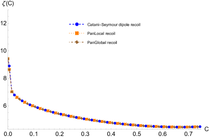
Figure 25: Fixed order calculation of $\zeta(C)$ with different recoil schemes Luisoni:2020efy .

A precise extraction of $\alpha_{S}$ with the above $\zeta(C)$ profile and further in depth studies of the interplay of the nonperturbative corrections discussed in this note with perturbative aspects of the calculation at higher orders are still necessary in order to make conclusive statements on the impact of the developments discussed in this note. Furthermore, similar studies for other event shape observables such as thrust (also addressed in Ref. Caola:2021kzt ) will be essential to shed more light on the current discrepancies among the different event-shape based extractions of $\alpha_{S}$ considered in the world average PDGQCD2019 .

4 The strong coupling from groomed event shapes

Event-shape variables such as thrust have been measured with high precision by the LEP experiments. These observables have played and continue to play an important role in the determination of the value of the strong coupling, see for instance Bethke:2009ehn ; Dissertori:2009ik ; Dissertori:2009qa ; OPAL:2011aa ; Schieck:2012mp ; Davison:2009wzs ; Abbate:2010xh ; Gehrmann:2012sc ; Abbate:2012jh , as well as the discussion in this report. While event shapes can be calculated with astonishing precision within perturbative QCD, both at fixed-order and resummed levels, nonperturbative contributions in particular due to hadronization can be sizable and thus affect the ultimate precision achievable. In the context of jet-substructure analyses of final states produced in hadronic collisions the soft-drop grooming technique offers a handle to reduce nonperturbative corrections Larkoski:2014wba . This idea can be transferred to (global) event shapes in lepton Baron:2018nfz and hadron collisions Baron:2020xoi . With a possibly reduced impact of nonperturbative contributions this can offer an improved precision in extractions of $\alpha_{S}$. In Ref. Marzani:2019evv this has been explored for the soft-drop version of thrust in ${\rm e^{+}e^{-}}$ collisions at $\sqrt{s}=m_{\mathrm{Z}}$.

The soft-drop variant of thrust (and similarly for other event shapes) is defined by first determining the conventional thrust axis and accordingly separating a given event into two hemispheres. The soft-drop procedure is then applied to both hemispheres independently. Soft-drop thrust is calculated based on the remaining constituents of both hemispheres, according to

$$\tau_{\text{SD}}=\frac{\sum_{i\in\mathcal{E}_{\text{SD}}}\left|\vec{p}_{i}\right|}{\sum_{i\in\mathcal{E}}\left|\vec{p}_{i}\right|}\left[1-\frac{\sum_{i\in\mathcal{H}^{L}_{\text{SD}}}\left|\vec{n}_{L}\cdot\vec{p}_{i}\right|+\sum_{i\in\mathcal{H}^{R}_{\text{SD}}}\left|\vec{n}_{R}\cdot\vec{p}_{i}\right|}{\sum_{i\in\mathcal{E}_{\text{SD}}}\left|\vec{p}_{i}\right|}\right],$$ (143)

where $\vec{n}_{L/R}$ denote the axes for the left and the right hemispheres, respectively, and the sums extend over all particles in the full event ($\mathcal{E}$), the soft-dropped event ($\mathcal{E}_{\text{SD}}$) or the left and right hemispheres ($\mathcal{H}^{L/R}$). Thereby, the ${\rm e^{+}e^{-}}$ version of soft drop operates on the hemispheres defined by the thrust axis, reclusters them using the Cambridge–Aachen algorithm and discards soft subjets failing the criterion

$$\frac{\text{min}(E_{i},E_{j})}{E_{i}+E_{j}}>z_{\text{cut}}(1-\cos\theta_{ij})^{\beta/2}\,.$$ (144)

While the parameter $z_{\text{cut}}$ determines how stringent the cut on the subjet energies is, $\beta$ provides an angular suppression to grooming.

Though originally designed to reduce nonperturbative effects like what is usually accounted for in multiple parton interaction (MPI) and underlying event (UE) simulations at hadron colliders Buckley:2011ms , soft drop has been shown to also significantly reduce the impact of hadronization corrections in event shapes and jet observables at lepton colliders in Baron:2018nfz . The viability of using soft-drop thrust in fits of $\alpha_{S}$ was studied in detail in Marzani:2019evv . Theoretical predictions computed at NLO+NLL^′ accuracy were employed in fits to hadron-level pseudodata generated with Sherpa Sherpa:2019gpd based on merging the NLO QCD matrix elements for ${\rm e^{+}e^{-}}\to 2,3,4,5$ partons with the dipole shower Schumann:2007mg , using a nominal value of $\alpha_{S}(m^{2}_{\mathrm{Z}})=0.117$, and the cluster-fragmentation model Winter:2003tt . The main results of this study are summarized in Fig. 26.

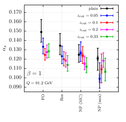
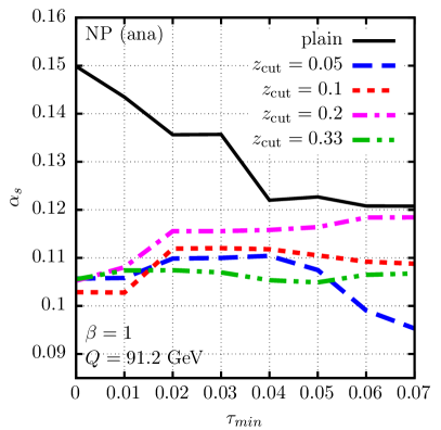
Figure 26: Results of Marzani:2019evv illustrating the advantages of using soft-drop thrust in fits of $\alpha_{S}$. Both are based on fits to pseudodata generated with Sherpa. Left: Dependence of the results on the effects included in the calculation, starting from only fixed order, i.e. NLO QCD, on the left and including effects of resummation, corresponding to NLO+NLL^′ accuracy, and upon including nonperturbative effects in two different approaches. Right: Dependence of the $\alpha_{S}$ best-fit value on the range of (soft-drop) thrust included in the fit.

Firstly, the results obtained from fitting $\alpha_{S}$ in the NLO+NLL^′ prediction for the soft-drop thrust distribution depend less strongly on nonperturbative effects than for plain thrust when using the same Monte Carlo (MC) pseudodata. This is illustrated in the left plot of Fig. 26. While the best-fit $\alpha_{S}$ values obtained from plain thrust change significantly when going from using fixed-order (FO) results to including resummation effects (Res) and again when including nonperturbative (NP) effects, either extracted from MC simulations or from an analytic model (ana). This change is reduced when considering soft-drop thrust, shown in Fig. 26 for $\beta=1$ and a variety of $z_{\text{cut}}$ values. Note, in Ref. Marzani:2019evv also the cases $\beta=0$ and $\beta=2$ have been considered.

Secondly, for soft-drop thrust the value of $\alpha_{S}$ obtained from the fits is less affected by the choice of the considered observable range. This is illustrated in the right plot of Fig. 26. The minimal observable value $\tau_{\text{min}}$ included in the fit is lowered from the default value $\tau_{\text{min}}=0.07$. The upper boundary is thereby kept fixed at $\tau_{\text{max}}=0.25$. For plain thrust, this results in dramatic changes due to increasing and severe hadronization corrections. Consequently, for plain thrust this additional observable range, i.e. phase-space region, can not reliably be used in an $\alpha_{S}$ extraction. However, the results obtained from soft-drop thrust, with the various choices of $z_{\text{cut}}$, are significantly more stable and the fit range could be extended into those areas.

From an experimental point of view, an obvious problem is that soft-drop event shapes have not been measured by the LEP experiments. However, their data are preserved and have recently been reanalysed for other observables Fischer:2015pqa ; Kluth:2017xai ; Chen:2021iyj ; Chen:2021uws . Thus, we believe, it would be very interesting to measure soft-drop event shapes, as well as broader families of (groomed) substructure observables like angularities or energy correlation functions, on archived LEP data and use them to perform novel fits of the strong coupling. On the other hand, soft-drop groomed event shapes can also be studied in hadron collisions Baron:2020xoi , so analogous analyses could be performed at the currently running LHC experiments. The same comment applies to analyses of soft-drop groomed jet substructure observables, see for example Caletti:2021oor ; CMS:2021iwu ; ALICE:2021njq ; Caletti:2021ysv ; Zhu:2021xjn ; Reichelt:2021svh ; Makris:2021drz for recent theoretical and experimental results. However, it should be noted that the study in Proceedings:2018jsb identified a strong correlation between $\alpha_{S}$ and the overall structure of the hard collision, in particular the fraction of quarks and gluons that enter the calculation, as one of the main challenges for extractions of $\alpha_{S}$ from jet-shape measurements in proton-proton collisions. Thus, in this context, it would be important to find observables that can break this degeneracy.

On the theory side, we also anticipate that higher-accuracy calculations will be necessary to be competitive with fits using traditional event shapes. At fixed order, NNLO accurate predictions are in principle available Kardos:2018kth . Furthermore, resummed predictions for soft-drop observables have been obtained at NNLL Frye:2016aiz and some results are available even at N³LL Kardos:2020gty . Regarding all-orders soft-gluon effects, a crucial ingredient is an improved understanding of the transition region where emissions soft enough to be groomed become important for the distribution. The resummed calculations like the ones used in Marzani:2019evv are performed in the strict $\tau\ll z_{\text{cut}}\ll 1$ limit. However, judging from the ranges where $\alpha_{S}$ has been extracted from LEP data of the thrust distribution, and assuming a traditional choice of $z_{\text{cut}}\sim{\cal{O}}(0.1)$, it seems however inevitable that a fit would also rely on the region $\tau\lesssim z_{\text{cut}}$ or even $\tau\sim z_{\text{cut}}$. Extending calculations to this region has been discussed recently in Benkendorfer:2021unv . With this, NNLL accuracy appears to be achievable over the whole range, however still limited to the assumption $z_{\text{cut}}\ll 1$. A better understanding of those power corrections in $z_{\text{cut}}$ is still a missing ingredient to date.

Finally, despite the fact that soft drop successfully reduces the sensitivity to nonperturbative effects, calculations aimed at precision determinations of the strong coupling cannot neglect them. In this context, significant improvement has been recently achieved, both in the analytic and MC approaches. Using effective field theory techniques, a more detailed understanding of power corrections due to hadronization in the presence of soft-drop grooming has been achieved in Refs. Hoang:2019ceu ; Pathak:2020iue . The Monte Carlo approach has also been improved thanks to the implementation of so-called transfer matrices Reichelt:2021svh . This method allows us to better model the effect that the hadronization process has on the event kinematics, although it was shown in Marzani:2019evv to not significantly alter the effect of nonperturbative corrections in the range of soft-drop thrust used for the central fits, like the ones in the left plot of Fig. 26. However, outside of this range, differences might be sizable. In this context, it would be interesting to compare this improved numerical model with the aforementioned first-principle analysis.

VII $\alpha_{S}(m^{2}_{\mathrm{Z}})$ from hadronic final-states in e-p and p-p collisions

1 $\alpha_{S}$ from jet-production cross sections in neutral-current DIS using NNLO predictions

The measurements of jet-production cross sections in neutral-current deep-inelastic scattering (NC DIS) are performed at HERA in the Breit frame of reference and provide clean and precise measurements. The Breit frame is defined as a brick-wall frame, where in leading-order NC DIS the incoming parton, literally, bounces back from the photon wall. Consequently, once the outgoing partons have significant transverse momenta, the process is described by a $2\to 2$ photon-parton scattering process in pQCD and is proportional to $\mathcal{O}(\alpha_{S})$ in leading order. Progress in the antenna subtraction formalism enabled to perform predictions for single-inclusive jet and dijet production cross sections up to next-to-next-to-leading order (NNLO) in pQCD Currie:2016ytq ; Currie:2017tpe . Several measurements of inclusive jet and dijet cross section measurements from the H1 and ZEUS collaborations, from different run-periods and different kinematic ranges in $Q^{2}$, were already exploited for the determination of $\alpha_{S}$.

Methodology

The value of $\alpha_{S}(m^{2}_{\mathrm{Z}})$ is determined from HERA jet cross sections in a $\chi^{2}$-minimization procedure of NNLO predictions to data. After the application of the factorization theorem the pQCD predictions for jet cross sections are

$$\sigma=\sum_{k=q,\bar{q},g}\int\text{d}xf_{k}(x)\hat{\sigma}_{k}(x)\cdot c_{\text{had}}\,,$$ (145)

where $f_{k}$ denotes the parton-distribution functions, $\hat{\sigma}$ the partonic NNLO cross section, and $c_{\text{had}}$ nonperturbative correction factors which account for hadronization effects. Both components at the hard scale, $f_{k}$ and $\hat{\sigma}_{k}$, exhibit a sensitivity to $\alpha_{S}(m^{2}_{\mathrm{Z}})$, which can directly be seen when calculating the partial derivative $\tfrac{\partial\sigma}{\partial\alpha_{S}(m^{2}_{\mathrm{Z}})}$. In order to account for both $\alpha_{S}$-sensitive terms, a constant starting scale $\mu_{0}$ is introduced, similarly as in DGLAP-based PDF-fits, and consequently the PDFs $f_{k}$ are defined through their $x$-dependence at $\mu_{0}$ and evolved to the factorization scale using the DGLAP formalism, where also the $\alpha_{S}$-sensitivity in the DGLAP kernels is exploited in the fitting procedure. The evolution starting scale is chosen to be $\mu_{0}=20$ GeV. In a study by H1 it was observed, that the extracted values of $\alpha_{S}(m^{2}_{\mathrm{Z}})$ are rather insensitive to the exact choice of the starting scale, and that the predominant sensitivity to $\alpha_{S}(m^{2}_{\mathrm{Z}})$ arises from the NNLO coefficients $\hat{\sigma}$. The value of $\alpha_{S}(m^{2}_{\mathrm{Z}})$ is then determined by minimizing the $\chi^{2}$ expression based on log-normal probability distribution functions

$$\chi^{2}=\bm{r}^{T}(V_{\text{exp}}+V_{\text{had}}+V_{\text{PDF}})^{-1}\bm{r}~{}~{}~{}\text{using}~{}~{}~{}r_{i}=\log\sigma_{\text{data},i}-\log\sigma_{\text{pred.},i}\,,$$ (146)

where the covariance matrices are calculated from relative uncertainties of the data ($V_{\text{exp}}$), the hadronization factors ($V_{\text{had}}$) and the PDFs ($V_{\text{PDF}}$) and the cross sections $\sigma_{\text{data},i}$ and $\sigma_{\text{pred.},i}$ refer to data and the NNLO predictions (pred.) in a bin $i$, respectively. The PDF uncertainties are calculated from the eigenvectors or replicas of a given PDF set from an external analysis. Note, by including the PDF uncertainties in the $\chi^{2}$ expression, the fit exploits the same degrees of freedom as the respective PDF fit, and the PDFs become profiled in the minimization procedure. This procedure is de-facto equivalent to adding the HERA jet to the PDF fit, while contrary the $\alpha_{S}(m^{2}_{\mathrm{Z}})$ inference exploits exclusively the jet data and thus ensures a theoretically and experimentally cleaner determination of $\alpha_{S}(m^{2}_{\mathrm{Z}})$ than PDF fits, which mix different predictions and processes.

The NNLO predictions are obtained using the program NNLOJET Currie:2017tpe , which is interfaced Britzger:2019kkb to fastNLO Britzger:2012bs and Applgrid Carli:2010rw to enable repeated calculations with differing values for $\alpha_{S}(m^{2}_{\mathrm{Z}})$ and differing PDFs. The DGLAP evolution is done with QCDNUM Botje:2010ay or Apfelxx Bertone:2017gds , and the hadronization correction factors are provided by the experimental collaborations together with the data and are commonly determined using the MC event generators Djangoh Charchula:1994kf or Rapgap Jung:1993gf . The PDFs are obtained from NNPDF3.1 NNPDF:2017mvq and further PDF sets are studied Alekhin:2017kpj ; Dulat:2015mca ; Harland-Lang:2014zoa ; Abramowicz:2015mha and are used to define a so-called PDFset uncertainty. The renormalization and factorization scales are identified with $\mu^{2}=Q^{2}+p_{\mathrm{T}}^{2}$, where $p_{\mathrm{T}}$ is identified with the single-jet transverse momentum in case of inclusive jets, and with the average $p_{\mathrm{T}}$ of the two leading jets in case of dijet cross sections.

$\alpha_{S}$ from single-jet inclusive cross sections

The value of $\alpha_{S}(m^{2}_{\mathrm{Z}})$ was determined from inclusive jet cross sections from previously published data by H1 in Ref. H1:2017bml , and from H1 and ZEUS inclusive jet cross sections in Ref. Britzger:2019kkb . Both experiments employ the $k_{t}$ jet-algorithm with a distance measure $R=1.0$ and provide double-differential cross section data as functions of $Q^{2}$ and jet transverse momenta $p_{\mathrm{T}}^{\text{jet}}$. The combined analysis of the H1 data using NNLO predictions exploits five independent cross section measurements H1:2000bqr ; H1:2009pze ; H1:2010mgp ; H1:2014cbm ; H1:2016goa in the kinematic range of $5<Q^{2}<15\,000$ GeV² and $4.5<p_{\mathrm{T}}^{\text{jet}}<50$ GeV and yields a value of $\alpha_{S}(m^{2}_{\mathrm{Z}})=0.1157\,(10)_{\text{exp}}\,(36)_{\text{th}}$ H1:2017bml , where the first uncertainty comprises experimental uncertainties, and the second collects theoretical uncertainties from PDFs, hadronization and missing higher orders. The analysis of ZEUS inclusive jet cross sections exploits two data sets from the HERA-I running period ZEUS:2002nms ; ZEUS:2006xvn in the kinematic range $120<Q^{2}<20\,000\,$GeV² and yields $\alpha_{S}(m^{2}_{\mathrm{Z}})=0.1227\,(21)_{\text{exp}}\,(19)_{\text{th}}$ Britzger:2019kkb . Since H1 provides more data, and data at lower scales $\mu$, their experimental uncertainty is smaller as compared to the ZEUS result, while contrary the highly-sensitive low-scale data results in increased scale uncertainties.

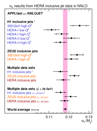
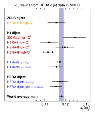
Figure 27: Left: $\alpha_{S}$ from HERA inclusive jet cross section measurements using NNLO pQCD predictions. Right: $\alpha_{S}$ from HERA dijet cross section measurements using NNLO pQCD predictions.

The combined analysis of H1 and ZEUS inclusive jet data yields the most precise result of Britzger:2019kkb

$$\alpha_{S}(m^{2}_{\mathrm{Z}})=0.1178\,(15)_{\text{exp}}\,(21)_{\text{th}}\,,$$ (147)

which is obtained by restricting the selected data to $\mu>28$ GeV. The NNLO predictions provide an excellent description of the data in all aspects and the value of $\chi^{2}/n_{\text{dof}}$ is found to be $79.2/104$. The dominant uncertainty arises from scale variations of the NNLO predictions, while several PDF-related uncertainties are found to be (negligibly) small. Future improved predictions may exploit these low-$\mu$ data and may achieve total uncertainties of less than $\pm 0.002$.

$\alpha_{S}$ from di-jet cross sections

A determination of $\alpha_{S}(m^{2}_{\mathrm{Z}})$ from dijet cross sections in NC DIS was performed by H1. Four previously published double-differential dijet cross section measurements as a function of $Q^{2}$ and the average transverse momenta of the two leading jets in the Breit frame $\langle p_{\mathrm{T}}\rangle$ were analyzed using NNLO pQCD predictions. The data were taken during different HERA run-periods, at different e^±-p center-of-mass energies and different kinematic regions in $Q^{2}$. From all four dijet data sets together a value of H1:2017bml

$$\alpha_{S}(m^{2}_{\mathrm{Z}})=0.1157\,(22)_{\text{exp}}\,(23)_{\text{th}}$$ (148)

is determined, and the fit exhibits an excellent quality with $\chi^{2}/n_{\text{dof}}=31.6/43$. While the above value is restricted to data with $\mu>28$ GeV, a determination from all dijet data yields $\alpha_{S}(m^{2}_{\mathrm{Z}})=0.1174\,(10)_{\text{exp}}\,(36)_{\text{th}}$. Hence, the experimental uncertainty would significantly be reduced, but contrary the theoretical uncertainties increase overly, which is due to enhanced sensitivity to $\alpha_{S}(m^{2}_{\mathrm{Z}})$ of data at lower scales and thus increased scale uncertainties.

An analysis of dijet cross section measurements from ZEUS exploits a single double-differential measurement ZEUS:2010vyw , as a function of $Q^{2}$ and $\langle p_{\mathrm{T}}\rangle$, where data were taken during HERA-I and HERA-II. However, its sensitivity to $\alpha_{S}(m^{2}_{\mathrm{Z}})$ is somewhat reduced, since the most sensitive data at low $\langle p_{\mathrm{T}}\rangle$ have to be omitted since the definition of the dijet observable causes instabilities of the pQCD predictions because of symmetric cuts on the two jets ZEUS:2010vyw ; Currie:2017tpe . The ZEUS dijet cross sections yield a value

$$\alpha_{S}(m^{2}_{\mathrm{Z}})=0.1156\,(34)_{\text{exp}}\,(25)_{\text{th}}\,.$$ (149)

Due to the limited sensitivity of the ZEUS dijet cross sections to $\alpha_{S}(m^{2}_{\mathrm{Z}})$, a combined analysis with H1 data does not improve over the H1 only result. For the future, a reanalysis of these data would be desirable, such that they can have a relevant impact on $\alpha_{S}(m^{2}_{\mathrm{Z}})$, and the analysis would profit from uncorrelated experimental uncertainties of the two independent experiments and high statistics.

$\alpha_{S}$ from jet cross sections of the H1 Collaboration

The H1 Collaboration performed a determination of $\alpha_{S}(m^{2}_{\mathrm{Z}})$ from inclusive jet and dijet data simultaneously using NNLO predictions. Although these observables are highly statistically correlated, this was made possible by a simultaneous analysis of inclusive jet and dijet data, where the statistical uncertainties and their correlations were measured as well H1:2014cbm ; H1:2016goa . The analysis further includes inclusive jet data from H1 from HERA-I and when restricting the data to $\mu>28$ GeV the result yields a value of H1:2017bml

$$\alpha_{S}(m^{2}_{\mathrm{Z}})=0.1166\,(19)_{\text{exp}}\,(24)_{\text{th}}\,.$$ (150)

Since the inclusive jet and dijet data are highly correlated, the result improves only moderately over the result from the respective inclusive jet data alone. The smallest experimental uncertainty is achieved with relaxed cut on $\mu$ and yields an experimental uncertainty of $\delta\alpha_{S}=\pm 0.0009$, which motivates future improved predictions to underbid the experimental precision.

a The running of $\alpha_{S}$ from HERA jet cross sections

Measurements of jet cross sections at HERA can be employed to test the running of the strong coupling, because these measurements cover a wide kinematic range. Once the renormalization scale $\mu_{r}$ is identified with final-state observables, every single cross section measurement of the double-differential data sets covers a well-defined range in $\mu_{r}$. Hence, determinations of $\alpha_{S}(m^{2}_{\mathrm{Z}})$ from selected data points with similar values of $\mu_{r}$ provide a determination of $\alpha_{S}$, where the validity of the renormalization group equation (RGE) is employed only within a limited $\mu_{r}$ range. The value of $\alpha_{S}(m^{2}_{\mathrm{Z}})$ can be translated to $\alpha_{S}(\mu_{r}^{2})$, using a representative value of $\mu_{r}$ of the selected data sets, and multiple measurements at different $\mu_{r}$ provide a test of the running of $\alpha_{S}$.

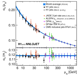
Figure 28: Left: Tests of the running of $\alpha_{S}$ using NNLO pQCD predictions together with H1 inclusive jet data, dijet data, or both together. The lower panel displays $\alpha_{S}(m^{2}_{\mathrm{Z}})$ as obtained in the fit to selected data points, and the upper panel the respective value of $\alpha_{S}(\mu_{r}^{2})$ for a representative value of $\mu_{r}$. The blue shaded band shows the expectation when assuming the world average value from PDG 2016. Right: A comparison of $\alpha_{S}(m^{2}_{\mathrm{Z}})$ and corresponding $\alpha_{S}(\mu_{r}^{2})$ from different measurements Baak:2014ora ; OPAL:2011aa ; Schieck:2012mp ; Dissertori:2007xa ; CMS:2016lna . Both figures taken from Ref. H1:2017bml .

The running of the strong coupling constant is tested using NNLO predictions together with inclusive jet and dijet data from H1 H1:2017bml , or solely inclusive jet data but from H1 and ZEUS were exploited Britzger:2019kkb , respectively. The $\overline{\text{MS}}$ renormalization scheme with 5 active flavors is used. Results from Ref. H1:2017bml are displayed in Fig. 28 and compared to the world average value and other determinations. Good consistency between results from inclusive jet and from dijet cross sections is observed, and all results are in good agreement with the world average value and the expectation from the RGE.

The HERA jet data are capable of testing the running of $\alpha_{S}$ in the range from about 7 to 90 GeV with a considerable precision of about 2.5 to 4 %.

b Further processes

In the recent years, the determination of $\alpha_{S}(m^{2}_{\mathrm{Z}})$ from e-p collision data focused mainly on inclusive jet and dijet data from HERA. This is because the recently achieved NNLO calculations Currie:2016ytq ; Currie:2017tpe provided a significant improvement over previously available NLO predictions H1:2017bml , and since H1 provided a comprehensive set of jet measurements from the HERA-II running period H1:2014cbm ; H1:2016goa . However, many further observables and final states can be exploited for $\alpha_{S}(m^{2}_{\mathrm{Z}})$, either once HERA data are further analyzed or when theoretical advancements are achieved.

Some examples, where future improvements could be possible, would be three-jet cross sections, heavy-flavor cross sections, event-shape observables, jet substructure observables or observables in photoproduction. As an example, three-jet cross sections from measurements by H1 were proven to provide small experimental uncertainties in $\alpha_{S}$ of about 1 % H1:2014cbm ; H1:2016goa , but only NLO Nagy:2001xb predictions are available and thus largely limit the precision, and no corresponding measurement from ZEUS is published either. Similarly, in photoproduction, a precision measurement of inclusive jet cross sections by ZEUS exhibits high sensitivity to $\alpha_{S}$ ZEUS:2012pcn , but no corresponding measurement from H1 is available, and no theoretical advancements were achieved for this process since then. The measurements of various event-shape observables in NC DIS by H1 H1:2005zsk and ZEUS ZEUS:2006vwm from HERA-I data proved a significant sensitivity to $\alpha_{S}$. However, although recent theoretical improvements were achieved Gehrmann:2019hwf and new calculation techniques and observables Kang:2013lga ; Kang:2013nha ; Kang:2015swk , or substructure Makris:2021drz could be studied, no suitable measurement of any such observable was published by the HERA experiments from HERA-II data (though, note the ongoing work in Ref. Hessler:2021usr ). A recent measurement of lepton-jet correlation observables in NC DIS H1:2021wkz , where the jets are defined in the laboratory rest-frame, may provide high sensitivity to $\alpha_{S}(m^{2}_{\mathrm{Z}})$, and also theoretical predictions with considerable precision are available.

c Future prospects

Future electron-proton collider experiments provide many opportunities for precision determinations of $\alpha_{S}$. At lower center-of-mass energies, the electron-ion collider in the USA (EIC) Accardi:2012qut ; AbdulKhalek:2021gbh and in China (EicC) Anderle:2021wcy will provide new high-luminosity data. Early studies investigate a measurement of the 1-jettiness global event shape observable and prospect a determination of $\alpha_{S}(m^{2}_{\mathrm{Z}})$ at a level of a few percent AbdulKhalek:2021gbh .

The proposed Large-Hadron-electron-Collider experiment at CERN (LHeC) LHeCStudyGroup:2012zhm ; LHeC:2020van will provide e^±-p collision data at a center-of-mass energy of 1.3 TeV and hence the measurements of hadronic final state observables cover a considerably larger range than it was possible at HERA. These data will provide new precision measurements of inclusive NC and CC DIS cross section data. Because of an excellent detector acceptance and high-luminosity, also the high-$x$ region will be measured with high precision. This will provide the opportunity to determine $\alpha_{S}$ from inclusive DIS data alone, something that was not possible with HERA data, and an experimental uncertainty of LHeC:2020van

$$\delta\alpha_{S}(m^{2}_{\mathrm{Z}})=\pm 0.00022\,\text{(exp+PDF)}\,,$$ (151)

can be expected in combined determination of PDFs and $\alpha_{S}(m^{2}_{\mathrm{Z}})$. The prospected uncertainties are compared with recent determinations in global PDF fits in Fig. 29.

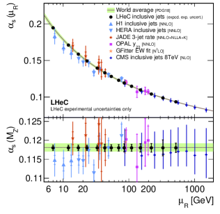
Figure 29: Left: Comparison of prospected determination of $\alpha_{S}(m^{2}_{\mathrm{Z}})$ from inclusive DIS data at the LHeC in comparison to determinations in (global) PDF fits. Right: An illustration of the prospected experimental uncertainties in a study of the running of $\alpha_{S}$ from inclusive jet cross sections at the proposed LHeC experiment. Both figs. taken from Ref. LHeC:2020van .

From a simulation of inclusive jet cross section data with a complete set of systematic uncertainties, a determination of $\alpha_{S}(m^{2}_{\mathrm{Z}})$ with uncertainties of

$$\delta\alpha_{S}(m^{2}_{\mathrm{Z}})=\pm 0.00013\,\text{(exp)}~{}\pm 0.00010\,\text{(PDF)}\,,$$ (152)

where the first uncertainties accounts for experimental uncertainties only and the second for PDF uncertainties, is expected in the LHeC/HL-LHC era. While experimental uncertainties can be well estimated, it is not quite possible to estimate the size of theoretical uncertainties reliably.

Similarly as at HERA, the running of $\alpha_{S}$ can be tested because of the dynamic scale of the jet data. Prospects for scale-dependent determinations of $\alpha_{S}(m^{2}_{\mathrm{Z}})$ (and corresponding values $\alpha_{S}(\mu_{r}^{2})$) are displayed in Fig. 29. It is observed, that from LHeC inclusive jet cross sections, the running can be tested in the range from a few GeV up to about 600 GeV with permille precision. These measurements will become an indispensable experimental confirmation of its validity, which will allow to combine the low-scale $\alpha_{S}$ determinations from $\tau$-decays or lattice QCD with those at the electroweak scale.

2 $\alpha_{S}(m^{2}_{\mathrm{Z}})$ from inclusive W and Z cross sections in p-p collisions

A new determination of $\alpha_{S}(m^{2}_{\mathrm{Z}})$ has been recently proposed dEnterria:2019aat ; CMS:2019oeb based on comparing the fiducial cross sections of electroweak (EW) boson production in p-p collisions at the LHC, $\mathrm{pp\to W,\,Z\,+\,X}$ (with the EW bosons decaying into clean final states with electrons or muons) to the corresponding theoretical cross sections computed at next-to-next-to-leading-order (NNLO) accuracy. The method employed follows a similar approach to that used to derive $\alpha_{S}(m^{2}_{\mathrm{Z}})$ from inclusive top-quark pair cross sections Klijnsma:2017eqp . Such an extraction exploits the fact that, first, there are many W and Z boson cross sections available and that those are the most precisely measured ones at the LHC (with typical $\pm 0.5\%$ statistical uncertainties and $\pm 2\%$ systematic uncertainties, dominated by the integrated luminosity), and, second, that their theoretical values can also be precisely computed (with scale and PDF uncertainties amounting to 0.5–1% and 2–-4%, respectively). Theoretically, the cross sections can be derived from the convolution of parton densities $f_{i}(x_{i},\mu_{F})$ (evaluated at fractional momentum $x_{i}$ and factorization scale $\mu_{F}$) and elementary parton-parton cross sections (evaluated at renormalization scale $\mu_{R}$) written as an expansion in the QCD coupling,

$$\!\!\sigma_{\rm pp\to W,Z+X}=\!\int\!\!\int\mathrm{d}x_{1}\mathrm{d}x_{2}\,f_{1}(x_{1},\mu_{F})f_{2}(x_{2},\mu_{F})\,\left[\hat{\sigma}_{\textsc{lo}}+\alpha_{S}(\mu_{R})\hat{\sigma}_{\textsc{nlo}}+\alpha_{S}^{2}(\mu_{R})\hat{\sigma}_{\textsc{nnlo}}+\cdots\right].$$ (153)

Although the bulk of the cross section, given by $\hat{\sigma}_{\textsc{lo}}$, is a pure EW quantity, the contributions of NLO and NNLO higher-order pQCD corrections increase the overall $\sigma_{\rm W,Z}$ value Anastasiou:2003ds ; Catani:2009sm ; Gavin:2010az ; Campbell:2010ff ; Boughezal:2016wmq , and provide the dependence on $\alpha_{S}(m^{2}_{\mathrm{Z}})$ that allows extracting this parameter from a combined data-theory comparison. The size of the higher-order corrections, encoded in the so-called K-factor given by the ratio of NNLO to LO cross sections, amounts to $\rm K=\sigma_{{}_{\rm NNLO}}/\sigma_{{}_{\rm LO}}\approx$ 1.22, 1.33, and 1.29 in the typical ATLAS, CMS, and LHCb fiducial acceptance for ${\rm W^{\pm}}$ and Z final states, respectively. Such a result indicates that indeed W and Z boson production in p-p collisions is sensitive to $\alpha_{S}(m^{2}_{\mathrm{Z}})$, through $\sim$25% higher-order matrix-elements direct contributions to their total cross sections.

Up to the year 2019, there were $12+9+7=28$ W^±and Z fiducial cross sections measured in p-p collisions by CMS, LHCb, and ATLAS, respectively, that have been exploited in dEnterria:2019aat ; CMS:2019oeb to determine $\alpha_{S}(m^{2}_{\mathrm{Z}})$ by comparing them to the corresponding NNLO theoretical predictions computed with mcfm v.8 Campbell:2010ff ; Boughezal:2016wmq for a variety of PDF sets (CT14 Dulat:2015mca , HERAPDF2.0 Abramowicz:2015mha , MMHT14 Harland-Lang:2014zoa , and NNPDF3.0 NNPDF:2014otw ) and $\alpha_{S}(m^{2}_{\mathrm{Z}})=0.115$–0.121 values. The absolute W^±and Z cross section data exploited here were not used by any of these PDF sets in their global fits to extract the parton densities themselves, so there is no “double counting” of the same data samples in the $\alpha_{S}(m^{2}_{\mathrm{Z}})$ determination. The final numerical accuracy of the calculations is 0.2–0.6%, comparable to $\sim$1% differences found with alternative NNLO calculators such as FEWZ Gavin:2010az or DYNNLO Catani:2009sm . In the theoretical cross sections, we included corrections (mostly negative, of a few percent size) due to EW and photon-induced production processes evaluated at NLO accuracy with mcsanc v.1.01 Bondarenko:2013nu .

Figure 30 shows examples of experimental ATLAS (left) and LHCb (right) cross sections (horizontal lines and bands) compared to the corresponding theoretical predictions per PDF as a function of $\alpha_{S}(m^{2}_{\mathrm{Z}})$ (coloured ellipses). From the computed cross sections, a linear dependence of $\sigma^{\mathrm{th}}_{\mathrm{W,Z}}$ on $\alpha_{S}(m^{2}_{\mathrm{Z}})$ is derived, and the filled ellipses are constructed to represent the contours of the joint probability density functions (Jpdfs) of the theoretical and experimental results, with a width representing a two-dimensional one standard-deviation obtained from the product of both probability densities for each PDF. The uncertainty in the theoretical cross sections is given by the quadratic sum of its associated PDF, scale, and numerical uncertainties. The predictions are consistent with data within uncertainties but not systematically for the same $\alpha_{S}(m^{2}_{\mathrm{Z}})$ value (in particular, HERAPDF2.0 results do not always overlap with any of the others within the 1 std.-dev. region). For a fixed $\alpha_{S}(m^{2}_{\mathrm{Z}})$ value, HERAPDF2.0 (NNPDF3.0) predict larger (smaller) cross sections. Namely, HERAPDF2.0 (NNPDF3.0) favour systematically smaller (larger) $\alpha_{S}(m^{2}_{\mathrm{Z}})$ values, whereas MMHT14 and CT14 predictions are in between and less scattered over the 28 measurements considered. The predictions derived with HERAPDF2.0 (MMHT14) always feature the smallest (largest) slope, i.e. HERAPDF2.0 (MMHT14) cross sections are the least (most) sensitive to underlying $\alpha_{S}(m^{2}_{\mathrm{Z}})$ variations. With the 28 fiducial cross sections computed, we find that for the baseline QCD coupling constant value of $\alpha_{S}(m^{2}_{\mathrm{Z}})=0.118$ of all PDF sets, the data-theory accord is overall better for the predictions calculated with CT14 and MMHT14 (goodness-of-fit per degree of freedom, $\chi^{2}/$ndf $\approx 1$) than those obtained with the HERAPDF2.0 and NNPDF3.0 sets ($\chi^{2}/$ndf $\approx 2.1$).

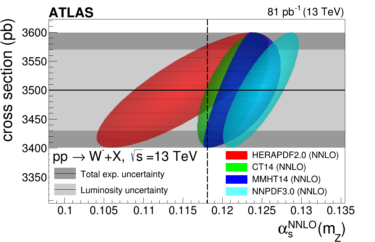
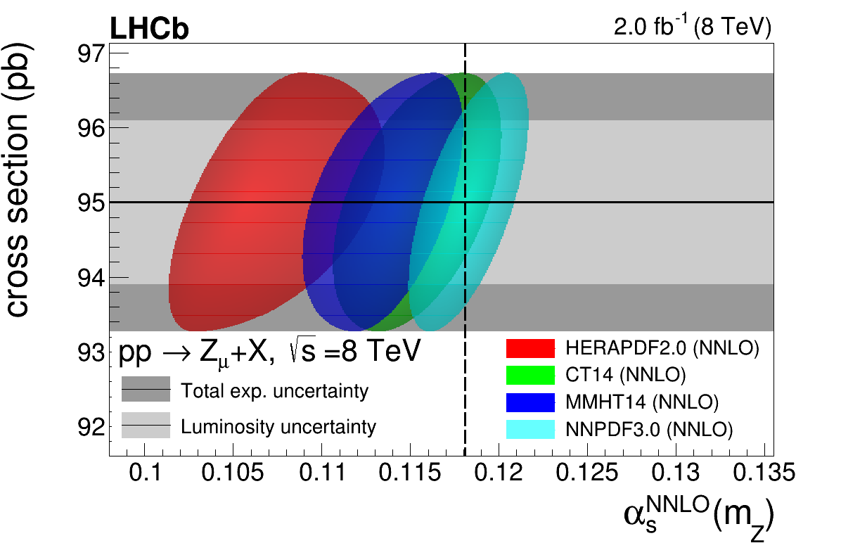
Figure 30: Examples of data-theory comparisons for EW fiducial cross sections in p-p collisions measured by ATLAS (W⁺ bosons at $\sqrt{s}=13$ TeV, left) ATLAS:2016fij and LHCb (Z boson at $\sqrt{s}=8$ TeV, right) LHCb:2015mad . The experimental cross sections are plotted as horizontal black lines with outer darker (inner grey) bands indicating their total (integrated luminosity) uncertainties. The theoretical predictions are computed for each PDF set as a function of $\alpha_{S}(m^{2}_{\mathrm{Z}})$, and combined with the experimental results into Jpdfs shown as filled ellipses. The vertical dashed line indicates the expected predictions for $\alpha_{S}(m^{2}_{\mathrm{Z}})=0.118$.

The cross sections calculated with different $\alpha_{S}(m^{2}_{\mathrm{Z}})$ values are fitted (using $\chi^{2}$-minimization) to a first-order polynomial and the corresponding slope $k$ is extracted for each PDF and measurement. The value of $\alpha_{S}(m^{2}_{\mathrm{Z}})$ preferred by each individual measurement is determined by the crossing point of the fitted linear theoretical curve with the experimental horizontal line. All the individual 28 $\alpha_{S}(m^{2}_{\mathrm{Z}})$ derived per PDF set, and the correlation matrices associated with all their uncertainties, are given as inputs of the convino v1.2 Kieseler:2017kxl program employed to determine the final best estimate of all combined values. Table 10 lists the $\alpha_{S}(m^{2}_{\mathrm{Z}})$ values, along with the uncertainty breakdowns from every source, determined for each PDF set through the combination of the 28 individual determinations. The total symmetrized uncertainties amount to $\sim$1.4% for CT14, $\sim$2.1% for HERAPDF2.0, $\sim$1.3% for MMHT14 and $\sim$1.6% for NNPDF3.0. The last column of Table 10 lists the ($\chi^{2}$/ndf) of the final single combined result compared to the 28 individual $\alpha_{S}(m^{2}_{\mathrm{Z}})$ extractions.

Table 10: Strong coupling constant $\alpha_{S}(m^{2}_{\mathrm{Z}})$ values extracted per PDF set by combining all the individual results obtained for each W^± and Z boson production cross section measurements, listed along with their propagated total and individual uncertainties. The last column tabulates the $\chi^{2}$/ndf of the final single combined result compared to the 28 individual $\alpha_{S}(m^{2}_{\mathrm{Z}})$ determinations.

PDF	$\alpha_{S}(m^{2}_{\mathrm{Z}})$	$\delta\,\text{(stat)}$	$\delta\,\text{(lumi)}$	$\delta\,\text{(syst)}$	$\delta$(PDF)	$\delta$(scale)	$\delta\,\text{(num)}$	$\chi^{2}$/ndf
CT14	$0.1172^{+0.0015}_{-0.0017}$	0.0003	0.0005	0.0006	${}^{+0.0011}_{-0.0013}$	0.0006	0.0003	23.5/27
HERAPDF2.0	$0.1097^{+0.0022}_{-0.0023}$	0.0004	0.0009	0.0009	${}^{+0.0015}_{-0.0016}$	0.0007	0.0005	27.0/27
MMHT14	$0.1188^{+0.0019}_{-0.0013}$	0.0002	0.0008	0.0003	${}^{+0.0015}_{-0.0007}$	0.0007	0.0002	19.3/27
NNPDF3.0	$0.1160\pm 0.0018$	0.0006	0.0004	0.0005	0.0013	0.0006	0.0007	56.9/27

The final $\alpha_{S}(m^{2}_{\mathrm{Z}})$ values determined for each individual PDF are plotted in Fig. 31 (left) compared with the 2018 world average of $\alpha_{S}(m^{2}_{\mathrm{Z}})=0.1181\pm 0.0011$ (orange band) ParticleDataGroup:2018ovx . The (asymmetric) parabolas are constructed to have a minimum at the combined value and are fitted to go through $\Delta\chi^{2}=1$ (horizontal black lines) at the one std. deviation uncertainties quoted in Table 10. The robustness and stability of the final $\alpha_{S}(m^{2}_{\mathrm{Z}})$ determination per PDF is cross-checked by varying key experimental and theoretical ingredients and uncertainties. For this purpose, the convino combination is redone as follows: (i) for a fraction of the data subsets (ATLAS, CMS, or LHCb alone; or for 7, 8, 13 TeV c.m. energies only), (ii) varying the correlation factors of the PDF/scale uncertainties between 0 and 1, (iii) shifting the central values of the computed cross sections by $\pm 1\sigma$ of the theoretical uncertainty prior to combination, and (iv) adding $\pm 1\%$ uncorrelated theoretical uncertainty (to cover differences among NNLO calculators). The results of such tests indicate that the MMHT14 result is the most stable against any variations in the analysis, whereas a few larger-than-1-standard-deviation changes appear in some cases for the results of the other PDF sets. The preferred QCD coupling value extracted from this study is that of MMHT14, $\alpha_{S}(m^{2}_{\mathrm{Z}})=0.1188\pm 0.0016$ plotted in Fig. 31 (right), because (i) it features the largest sensitivity (slope) of $\sigma_{\mathrm{W,Z}}$ to $\alpha_{S}$, (ii) it shows the lowest $\chi^{2}$/ndf of the final single combined result compared to the 28 individual $\alpha_{S}(m^{2}_{\mathrm{Z}})$ extractions, (iii) it has the smallest (symmetrized) propagated uncertainties, and (iv) it is the most stable against any data or theory analysis variations.

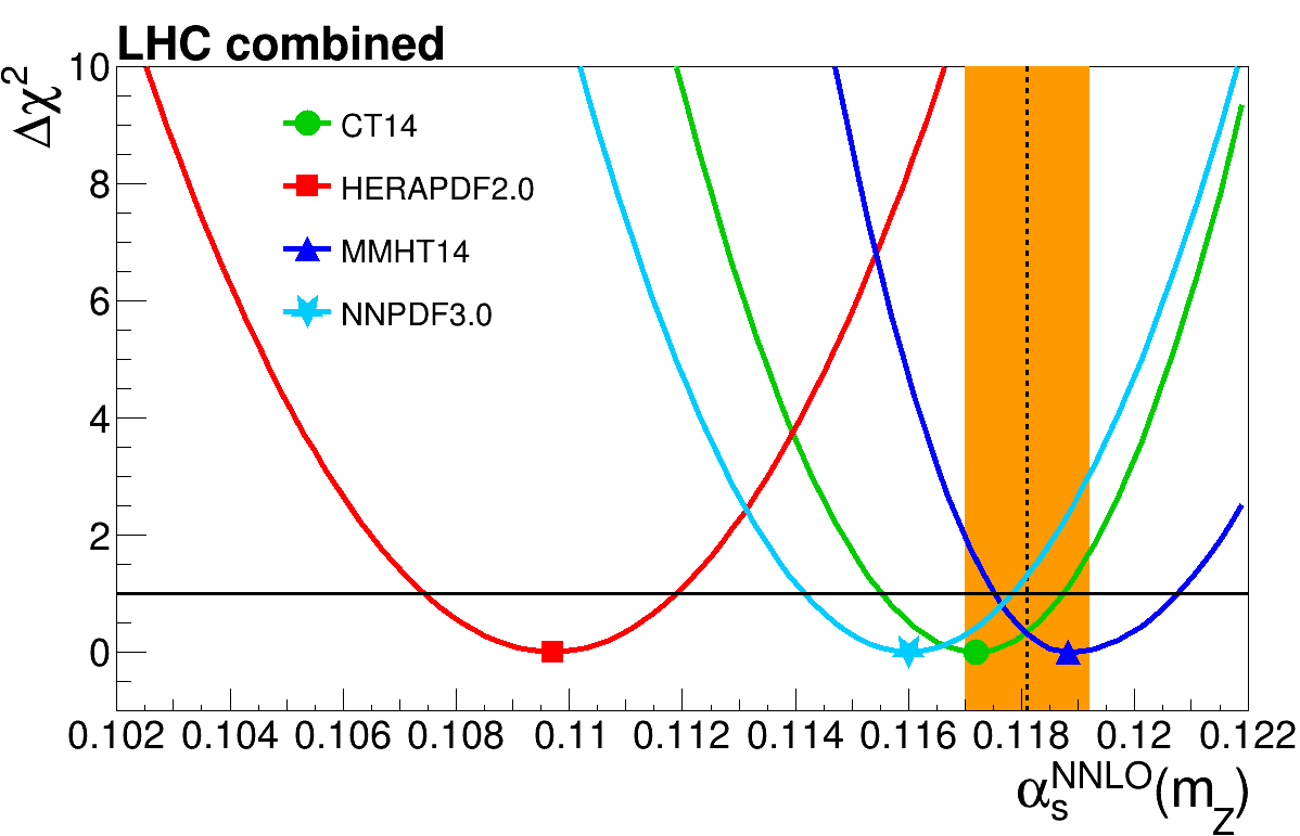
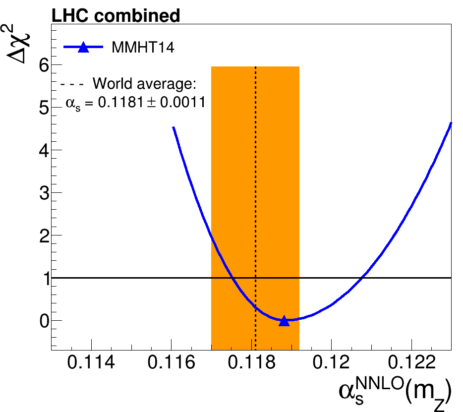
Figure 31: Final $\alpha_{S}(m^{2}_{\mathrm{Z}})$ values determined from the analysis of the EW boson inclusive cross sections at the LHC using the CT14, HERAPDF2.0, MMHT14, and NNPDF3.0 PDF sets (left), and $\alpha_{S}(m^{2}_{\mathrm{Z}})$ extraction from the MMHT14 PDF alone (right), compared to the 2018 world average (vertical orange band).

This study confirms that the total inclusive ${\rm W^{\pm}}$ and Z boson cross sections at hadron colliders are new promising observables that can provide useful constraints on the value of the QCD coupling constant, and that can eventually help improve the precision of the $\alpha_{S}(m^{2}_{\mathrm{Z}})$ world average. The recent availability of N³LO codes Duhr:2020sdp ; Camarda:2021ict for the calculation of inclusive ${\rm W^{\pm}}$ and Z boson production cross sections, with one extra higher degree of theoretical accuracy compared to the one used here, will allow for further reductions of the propagated scale uncertainties, provided that PDF uncertainties are available at the same level of pQCD accuracy. Such theoretical developments, combined with upcoming EW boson measurements at the LHC with $\mathcal{O}($1%) experimental uncertainties, mostly thanks to further reduced integrated luminosity uncertainties, will enable future $\alpha_{S}(m^{2}_{\mathrm{Z}})$ extractions with propagated uncertainties below the 1% level.

3 $\alpha_{S}(m^{2}_{\mathrm{Z}})$ from the transverse-momentum distribution of Z bosons

A new determination of $\alpha_{S}(m^{2}_{\mathrm{Z}})$, using QCD resummed theory predictions and based on a semi-inclusive (i.e. radiation inhibited) observable at hadron-hadron colliders, has been recently proposed in Ref. Camarda:2022qdg . The strong-coupling constant $\alpha_{S}(m^{2}_{\mathrm{Z}})$ is determined from the transverse-momentum distribution of Z bosons measured at $\sqrt{s}=1.96$ TeV with the CDF experiment, using predictions based on $q_{\mathrm{t}}$-resummation at N³LO+N³LL accuracy, as implemented in the DYTurbo Camarda:2019zyx ; Camarda:2021ict program. The measurement is performed through a simultaneous fit of $\alpha_{S}(m^{2}_{\mathrm{Z}})$ and the nonperturbative Sudakov form factor.

This measurement has all the desirable features for a precise determination of $\alpha_{S}(m^{2}_{\mathrm{Z}})$: large observable’s sensitivity to $\alpha_{S}(m^{2}_{\mathrm{Z}})$ compared to the experimental precision; high accuracy of the theoretical prediction; small size of nonperturbative QCD effects.

Measuring $\alpha_{S}(m^{2}_{\mathrm{Z}})$, or equivalently $\Lambda_{\textrm{QCD}}^{\overline{\mathrm{MS}}}$, from semi-inclusive Drell–Yan cross sections was first proposed in Ref. Catani:1990rr , by using Monte Carlo parton showers to determine $\Lambda_{\textrm{QCD}}^{\textrm{MC}}$ and later convert it to $\Lambda_{\textrm{QCD}}^{\overline{\mathrm{MS}}}$. The conversion is based on resummation arguments showing that a set of universal QCD corrections can be absorbed in coherent parton showers by applying a simple rescaling, the so-called Catani-Marchesini-Webber (CMW) rescaling.

The Z-boson transverse-momentum distribution at small transverse momentum is one of such semi-inclusive observables. The recoil of Z bosons produced in hadron collisions is mainly due to QCD initial-state radiation, and the Sudakov form factor is responsible for the existence of a Sudakov peak in the distribution, at transverse-momentum values of approximately 4 GeV. The position of the peak is sensitive to the value of the strong-coupling constant.

For the measurement of $\alpha_{S}(m^{2}_{\mathrm{Z}})$ from the Z-boson transverse-momentum distribution it is necessary to rely on fast computing codes which allow the calculation of variations in the input parameters with small numerical uncertainties. To this end, the DYTurbo program was used.

The CDF measurement of Z-boson transverse-momentum distribution CDF:2012brb at the Tevatron collider is ideal for testing the extraction of $\alpha_{S}(m^{2}_{\mathrm{Z}})$ with DYTurbo predictions. This measurement was performed with the angular coefficients technique, which allows extrapolating the cross section to full-lepton phase space with small theoretical uncertainties. The full-lepton phase space cross section allows fast predictions and avoid any theoretical uncertainties on the modelling of the Z-boson polarisation. Another advantage of this measurement with respect to similar measurements performed at the LHC is the fact that Tevatron is a proton-antiproton collider, and the Z-boson production has reduced contribution from heavy-flavour-initiated processes compared to proton-proton collisions at the LHC.

The CDF measurement is performed in the electron channel, with central ($|\eta^{e}|<1.1$) and forward ($1.2<|\eta^{e}|<2.8$) electrons, allowing a coverage up to Z-boson rapidity of $y=2.8$, and a small extrapolation to the full rapidity range $|y_{\textrm{max}}|\approx 3.1$ of Z-boson production at $\sqrt{s}=1.96$ TeV. The data sample is characterised by low values of the average number of interactions per bunch crossing, and by good electron resolution, at the level of 1 GeV for central electrons, and 1.5 GeV for forward electrons. The good resolution allows fine transverse-momentum binning (0.5 GeV) while keeping the bin-to-bin correlations smaller than 30%.

The nonperturbative QCD corrections to the Z-boson transverse-momentum distribution are modelled by including a nonperturbative term in the Sudakov form factor: $S(b)\to S(b)\cdot S_{\textrm{NP}}(b)$. The general form of $S_{\textrm{NP}}(b)$ is mass and centre-of-mass energy dependent Landry:2002ix . However, at fixed invariant mass $q=m_{Z}$, and for one value of centre-of-mass energy, the form of $S_{\textrm{NP}}(b)$ can be simplified to depend on a single parameter $g$: $S_{\textrm{NP}}(b)=\exp(-g\cdot b^{2})$. The nonperturbative parameter $g$ is generally determined from the data, and its value depends on the chosen prescription to avoid the Landau pole in the impact-parameter b-space, which corresponds to a divergence of the Sudakov form factor. The divergence is avoided by using the so-called $b_{\star}$ prescription, which freezes $b$ at a given value $b_{\textrm{lim}}$: $b\to b_{\star}=\frac{b}{1+b^{2}/b_{\textrm{lim}}^{2}}$. In this analysis $b_{\textrm{lim}}$ is set to the value of 3 GeV^-1.

The sensitivity of the Z-boson transverse-momentum distribution to $\alpha_{S}(m^{2}_{\mathrm{Z}})$ mainly comes from the position of the Sudakov peak, and is related to the average recoil scale $\langle p_{\textrm{T}}\rangle\approx 10$ GeV. The sensitivity of the Z-boson transverse-momentum distribution to $g$ also comes from the position of the Sudakov peak. However the scale of the nonperturbative smearing governed by $g$ corresponds to the value of primordial $k_{\mathrm{T}}$. Typical values of $g\approx 0.6$ GeV² corresponds to a primordial $k_{\mathrm{T}}$ of approximately 1.5 GeV. It is possible to disentangle the perturbative contribution to the Sudakov form factor, governed by $\alpha_{S}(m^{2}_{\mathrm{Z}})$, from the nonperturbative one, determined by $g$, thanks to their different scale, as shown in Fig. 32.

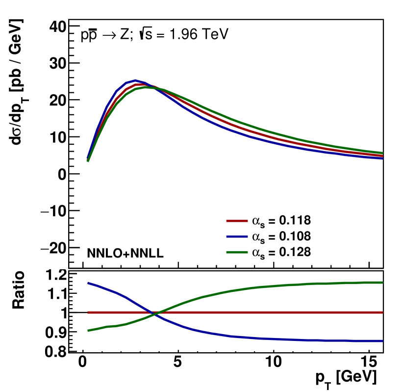
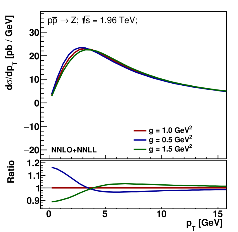
Figure 32: Sensitivity of the Z-boson transverse-momentum distribution to $\alpha_{S}(m^{2}_{\mathrm{Z}})$ (left) and to the nonperturbative QCD parameter $g$ (right).

The statistical analysis leading to the determination of $\alpha_{S}(m^{2}_{\mathrm{Z}})$ is performed by interfacing DYTurbo to xFitter Alekhin:2014irh . The agreement between data and predictions is assessed by means of a $\chi^{2}$ function, which includes experimental and PDFs theoretical uncertainties HERAFitterdevelopersTeam:2015cre . The nonperturbative form factor is added as unconstrained nuisance parameter in the $\chi^{2}$ definition, i.e. it is left free in the fit. The fit to the data is performed in the region of transverse momentum $p_{\textrm{T}}<30$ GeV by minimising the $\chi^{2}$ as a function of $\alpha_{S}(m^{2}_{\mathrm{Z}})$, with $\alpha_{S}$ variations as provided in LHAPDF.

The corrections to the Z-boson transverse-momentum distribution due to QED initial-state radiation are estimated with Pythia8 and the AZ tune ATLAS:2014alx of the parton shower parameters, and applied as multiplicative corrections. They are the level of 1%, and are responsible for a shift in the measured value of $\alpha_{S}(m^{2}_{\mathrm{Z}})$ of $\delta\alpha_{S}(m^{2}_{\mathrm{Z}})=-0.0004$.

The determination of $\alpha_{S}(m^{2}_{\mathrm{Z}})$ with the NNLO NNPDF4.0 PDF set Ball:2021leu yields $\alpha_{S}(m^{2}_{\mathrm{Z}})=0.1187$, with a statistical uncertainty of $\pm 0.0007$, a systematic experimental uncertainty of $\pm 0.0001$, and a PDF uncertainty of $\pm 0.0004$. The value of $g$ determined in the fit is $g=0.66\pm 0.05$ GeV², and the value of the $\chi^{2}$ function at minimum is 41 per 53 degrees of freedom. Various alternative NNLO PDF sets are considered: CT18 Hou:2019efy , CT18Z, MSHT20 Bailey:2020ooq , HERAPDF2.0 Abramowicz:2015mha , and ABMP16 Alekhin:2017kpj . The determined values of $\alpha_{S}(m^{2}_{\mathrm{Z}})$ range from a minimum of 0.1178 with the ABMP16 PDF set to a maximum of 0.1192 with the CT18Z PDF set. The midpoint value in this range of $\alpha_{S}(m^{2}_{\mathrm{Z}})=0.1185$ is considered as nominal result, and the PDF envelope of $\pm 0.0007$ as an additional source of uncertainty. Missing higher order uncertainties are estimated through independent variations of $\mu_{R}$, $\mu_{F}$ and $Q$ in the range $m_{\ell\ell}/2\leq\{\mu_{R},\mu_{F},Q\}\leq 2m_{\ell\ell}$ with the constraints $0.5\leq\{\mu_{F}/\mu_{R},Q/\mu_{R},Q/\mu_{F}\}\leq 2$, leading to 14 variations. The determined values of $\alpha_{S}(m^{2}_{\mathrm{Z}})$ range from a minimum of 0.1177 to a maximum of 0.1193, yielding a scale-variation envelope of $\pm 0.0008$. Alternative fits with a value of $b_{\textrm{lim}}=2$ GeV^-1 in the $b_{*}$ regularization procedure and with the minimal prescription yields an uncertainty of ${}^{+0.0006}_{-0.0004}$. A fit in which the NNPDF4.0 PDF set is evolved with a variable-flavour number scheme yields $\delta\alpha_{S}(m^{2}_{\mathrm{Z}})=-0.0002$. The stability of the results upon variations of the fit range is tested by performing fits in the regions of Z-boson transverse momentum $p_{\mathrm{T}}<20$ GeV and $p_{\mathrm{T}}<40$ GeV. The spread in the determined values of $\alpha_{S}(m^{2}_{\mathrm{Z}})$ is at the level of $\pm 0.0001$ and is not considered as a source of uncertainty. Since the region $20<p_{\mathrm{T}}<40$ GeV is sensitive to the matching of the resummed cross section to the fixed order prediction, this test provides a strong confirmation that the missing O($\alpha_{S}^{3}$) contributions to the asymptotic term and the $V$+jet finite-order cross section are negligible for this analysis. The measured value of the strong-coupling constant is $\alpha_{S}(m^{2}_{\mathrm{Z}})=0.1185^{+0.0015}_{-0.0014}$, with a statistical uncertainty of $\pm 0.0007$, an experimental systematic uncertainty of $\pm 0.0001$, a PDF uncertainty of $\pm 0.0008$, missing higher order uncertainties of $\pm 0.0008$, and additional theory uncertainties of ${}^{+0.0007}_{-0.0004}$. The post-fit predictions are compared to the measured Z-boson transverse-momentum distribution in Fig. 33 (left).

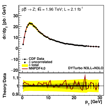
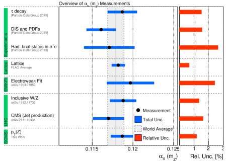
Figure 33: Left: Comparison of the N³LO+N³LL DYTurbo prediction to the measured Z-boson transverse-momentum distribution. Right: Comparison of the $\alpha_{S}(m^{2}_{\mathrm{Z}})$ derived here to the results of other categories of the world-average value.

We make some observations on this determination of $\alpha_{S}(m^{2}_{\mathrm{Z}})$. Contrary to other hadron collider observable, the Z-boson transverse-momentum distribution in the Sudakov region is not included in PDF fits, therefore this determination does not have any issue of correlation with existing PDF sets. The PDF uncertainties are estimated with a conservative approach, including the envelope of six different PDF sets. Missing higher order uncertainties are estimated with the standard approach of computing an envelope of scale variations. The model for nonperturbative QCD effects based on a Gaussian form factor is simple but effective, as it describes the data very well. Generous uncertainties on this model are estimated with variations of the Landau pole prescription. The measured value of $\alpha_{S}(m^{2}_{\mathrm{Z}})$ has a relative uncertainty of $1.2\%$, and is compatible with other determinations and with the world-average value, as illustrated in Fig. 33 (right).

Finally, we outline our personal wish-list for experimental and theoretical developments. LHC measurement of Z-boson transverse-momentum distributions are significantly more precise than measurements at the Tevatron. By analysing LHC data it is likely to reach a few $10^{-4}$ experimental uncertainty on $\alpha_{S}(m^{2}_{\mathrm{Z}})$ with the LHC Run-2 and Run-3 data samples. The main experimental limitation will be the lepton momentum/energy scale, currently known at $\sim 10^{-3}$. Improving the lepton scale to $10^{-4}$ will help to reach high precision on $\alpha_{S}(m^{2}_{\mathrm{Z}})$. Measurements of Drell–Yan transverse-momentum distributions at high mass will bring further sensitivity to $\alpha_{S}(m^{2}_{\mathrm{Z}})$, but resolution may be a limiting factor. Precise measurements of Drell–Yan transverse-momentum at low and intermediate masses will help reducing the nonperturbative uncertainties.

From the point of view of theory predictions, the analysis will clearly benefit from even higher order predictions. The N⁴LL accuracy is likely to be possible in the near future, and approximate N⁴LL’ could also be on reach in the coming years. The required ingredients for N⁴LL are the 5-loop cusp anomalous dimension, the 4-loop rapidity anomalous dimension. For N⁴LL’ also N³LO PDFs, N⁴LO TMD, and the 4-loop quark form factor are needed. In order to make full usage of the extremely precise LHC measurements, it is needed to have an improved heavy-flavour treatment, with variable-flavour number scheme and/or massive corrections. The inclusion of joint $q_{\mathrm{T}}$/small-$x$ resummation Marzani:2015oyb may also be relevant or even required. The precision of the measurement will greatly benefit from first-principle understanding of nonperturbative corrections. As a last remark, the availability of public software for Z+jet predictions at NNLO would help the inclusion of currently missing O($\alpha_{S}^{3}$) terms in the matching to fixed order. In conclusion, prospects to reach subpercent precision in the next 5–10 years mostly rely on theory developments.

4 Crucial aspects of PDF fits relevant for $\alpha_{S}(m^{2}_{\mathrm{Z}})$ determination

Parton densities uncertainties play an important role in $\alpha_{S}(m^{2}_{\mathrm{Z}})$ determinations from hadron collider measurements. A novel analysis at NNLO accuracy for the determination of a new set of proton PDFs using diverse measurements in p-p collisions at $\sqrt{s}$ = 7, 8 and 13 TeV performed by the ATLAS experiment at the LHC, and combined with DIS data from e-p collisions at the HERA collider, has been presented in Ref. ATLAS:2021vod with the resulting set of PDFs called ATLASpdf21. In this analysis, particular attention is paid to the correlation of systematic uncertainties within and between the various ATLAS data sets and to the inclusion of theoretical scale uncertainties, two crucial aspects of PDF fits if an ultimate precision of $\mathcal{O}(1\%)$ is sought on PDFs determination.

Specifically, the correlations of various systematic sources have been considered between different analyses that use jet data: $t\overline{t}$ data in the lepton+jets channel ATLAS:2015lsn ; ATLAS:2019hxz , W/Z $+$ jets data ATLAS:2017irc ; ATLAS:2019bsa , and inclusive jet data ATLAS:2017kux . The difference in the resulting $x\bar{d}$ and gluon $xg$ PDFs when such correlations between the input data sets are considered and when they are not is shown in Fig. 34. Such differences are still visible at LHC energy scales, indeed this figure is made for the scale $Q^{2}=10^{4}$ GeV² to illustrate so.

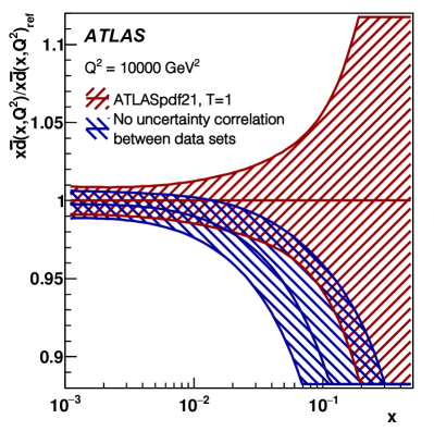
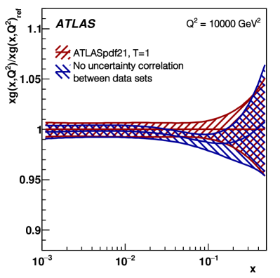
Figure 34: Difference in the gluon and the $x\bar{d}$ PDFs shown in ratio to the ATLASpdf21 (default) PDFs at scale $Q^{2}$ = 10⁴ GeV². The default (red) analysis applies the full correlation of specified systematic sources between the data sets which use jet data, and the alternative (blue) analysis does not apply any correlation of systematics sources between the data sets (apart from the luminosities).

It is visible how correlations of sources of systematic uncertainty both within and between data sets need to be carefully considered in PDF fits and although the difference between the resulting PDFs is not large in the best known kinematic region (namely $0.01<x<0.1$, corresponding to mass scales $\sim$100 GeV $\to$ 1 TeV at the LHC) it can nevertheless be large enough to have impact. In the less well-known regions, at smaller and larger mass scales, the impact can be considerably greater.

Another important aspect to be considered is the inclusion of theoretical scale uncertainties, which are evaluated as follows. The $K$-factors are evaluated for separate changes of the renormalisation ($\mu_{R}$) and factorisation ($\mu_{F}$) scales by factors of 2 and 0.5. The magnitude of the $K$-factor difference is symmetrised as $(K[\mu_{R}(2)]-K[\mu_{R}(0.5)])/2$ and ($K[\mu_{F}(2)]-K[\mu_{F}(0.5)])/2$ and its sign is preserved as positive if the upward variation of $\mu_{R}$ or $\mu_{F}$ makes the $K$-factor increase, and negative if it makes the $K$-factor decrease. In the ATLASpdf21 analysis, for the ATLAS W and Z$/\gamma^{*}$ inclusive data sets at both 7 and 8 TeV, both the total experimental uncertainty and the scale uncertainties approach $\sim 0.5\%$, so the scale uncertainties are considered as additional theoretical uncertainties (the effect of scale uncertainties for the other data sets entering in the fit was studied and was found to be negligible). Due to the similarity of the W and Z processes, both the $\mu_{R}$ and $\mu_{F}$ scales are considered correlated within the W, Z data sets at 7 TeV and between the W and Z data sets at 8 TeV. They are also considered to be correlated between the W and Z data sets at 7 and 8 TeV for the central fit.

Different choices for the treatment of the scale uncertainties in inclusive W, Z data are considered, and two alternative cases are considered:

• the scale uncertainties are not correlated between the 7 and 8 TeV data,

• scale uncertainties are not applied at all.

Fig. 35 shows the results of fits for these two cases, compared with the central fit, are shown as a ratio at a scale $Q^{2}$ = 10⁴ GeV², relevant for LHC physics. The uncertainties are very similar in size. The differences between the shapes of the PDFs are not large, but they can be important if the desired accuracy of the PDFs is $\mathcal{O}(1\%)$. The difference between the cases where the scale uncertainties are applied as being correlated or uncorrelated between the 7 and 8 TeV inclusive W, Z data sets is shown by the green line in these figures and it can be seen that it is generally a smaller effect.

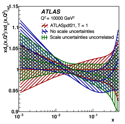
Figure 35: ATLASpdf21, showing the ratios of a fit not including theoretical scale uncertainties in the inclusive W, Z data to the central fit which does include these uncertainties, at the scale $Q^{2}$ = 10⁴ GeV². Left: $xd_{v}$. Right: $xg$.

The two aforedescribed effects should be taken into account properly when performing future precision data analyses, such as the measurement of $m_{\mathrm{W}}$, $\sin^{2}\theta_{\mathrm{W}}$ or $\alpha_{S}(m^{2}_{\mathrm{Z}})$, because fits to these quantities can be very sensitive to (even) small changes.

5 Exact fixed-order pQCD predictions for cross section ratios

In the standard approach, pQCD predictions for ratios of cross sections are computed as the ratio of the fixed-order predictions for the numerator and the denominator. Beyond the lowest order in the perturbative expansion, this result does, however, not correspond to a fixed-order prediction for the ratio. This contribution describes how exact fixed-order results for ratios of arbitrary cross sections can be obtained. Differences between the standard approach and the exact fixed-order results should be regarded as uncertainties of the predictions, related to possible higher-order contributions to the perturbative expansion. While this idea was motivated by our group’s $\alpha_{S}$ determinations from ratios of jet cross sections in hadron collisions (for which pQCD predictions are currently available up to NLO), the method can be applied at any order pQCD, for any processes, and arbitrary cross sections. The full details of the method are documented in Ref. Sawyer:2021bzn . Here, we describe the general method for the computation of the exact fixed-order results and provide specific results for the NLO and NNLO cases. For various multijet cross section ratios in hadron collisions that were previously used in $\alpha_{S}$ determinations, we compare the NLO pQCD predictions for the two methods, and study how they describe the experimental data.

A measurable quantity $R=\frac{\sigma_{n}}{\sigma_{d}}$ is defined as the ratio of two cross sections $\sigma_{n}$ and $\sigma_{d}$. It is assumed that the quantity $R$ is defined in bins of an energy or transverse momentum related variable $p$ which is defined for both $\sigma_{n}$ and $\sigma_{d}$. At a fixed value (or in a given bin) of $p$, the quantity $R$ is given by $R(p)=\frac{\sigma_{n}(p)}{\sigma_{d}(p)}$, and it is assumed that in a pQCD calculation the renormalization scale $\mu_{\mathrm{r}}$ can be related to $p$ by the same simple function (like $\mu_{\mathrm{r}}=p$ or $\mu_{\mathrm{r}}=p/2$) for both, $\sigma_{n}$ and $\sigma_{d}$. In other words, in a given bin of $p$, the ratio $R$ is probing $\alpha_{S}$ and the pQCD matrix elements for $\sigma_{n}$ and $\sigma_{d}$ at the same $\mu_{\mathrm{r}}$. For the sake of brevity, the dependence on $p$ is omitted in the following.

In phenomenological analyses of experimental data, the LO, NLO, and NNLO pQCD prediction for $R$ are usually computed from the ratios of the corresponding pQCD predictions for the numerator and denominator, $\sigma_{n}$ and $\sigma_{d}$, as

$$R_{\rm LO}=\frac{\sigma_{n,\rm LO}}{\sigma_{d,\rm LO}}\qquad\mbox{and}\qquad R_{\rm NLO}=\frac{\sigma_{n,\rm NLO}}{\sigma_{d,\rm NLO}}\qquad\mbox{and}\qquad R_{\rm NNLO}=\frac{\sigma_{n,\rm NNLO}}{\sigma_{d,\rm NNLO}}\,.$$ (154)

While the LO pQCD prediction for $R$ is uniquely defined, the higher-order pQCD predictions can be obtained in different ways. In the following, we refer to the above results as as the “standard” approach. Note that, beyond LO, these ratios are not exact fixed-order pQCD results for the quantity $R$.

We write the perturbative expansion for $\sigma_{n}$ as $\sigma_{n}=\sigma_{n,\rm LO}\cdot(1+k_{n,1}+k_{n,2}+...)$ where $k_{n,1}$ is related to the NLO correction ($k_{n,1}=\frac{\sigma_{n,\rm NLO}-\sigma_{n,\rm LO}}{\sigma_{n,\rm LO}}$) and $k_{n,2}$ to the NNLO correction ($k_{n,2}=\frac{\sigma_{n,\rm NNLO}-\sigma_{n,\rm NLO}}{\sigma_{n,\rm LO}}$). The variables $k_{n,i}$ for $i\geq 3$ (corresponding to corrections beyond NNLO) are defined correspondingly, and also the corresponding variables $k_{d,i}$ $i\geq 1$ for the denominator $\sigma_{d}$. The ratio $R$ is then given by

$$R=R_{\rm LO}\cdot\left(1+k_{n,1}+k_{n,2}+\cdots\right)\cdot\left(1+k_{d,1}+k_{d,2}+\cdots\right)^{-1}\,.$$

To obtain an exact fixed-order result for $R$, the second parenthesis is expanded in a Taylor series $(1+x)^{-1}=1-x+x^{2}-x^{3}+\cdots$ with $x=k_{d,1}+k_{d,2}+\cdots$. The terms of this series are multiplied with the terms in the left parenthesis, and the resulting products of $k_{n,i}$ and $k_{d,j}$ are sorted in powers of $\alpha_{S}$. The infinite series is then truncated at the corresponding order at which $\sigma_{n}$ and $\sigma_{d}$ were computed. This is the general procedure by which exact fixed-order results for $R$ are obtained at arbitrary orders in pQCD. At NLO, (with $x=k_{d,1}$ in the Taylor series) this yields

$$R_{\rm NLO}=R_{\rm LO}\cdot(1+k_{n,1}-k_{d,1})\,,$$ (155)

and at NNLO (with $x=k_{d,1}+k_{d,2}$ in the Taylor series)

$$R_{\rm NNLO}=R_{\rm LO}\cdot\left[1+(k_{n,1}-k_{d,1})+(k_{n,2}-k_{d,2}-k_{d,1}(k_{n,1}-k_{d,1})\right]\,.$$ (156)

In the following discussion, these results are referred to as the “fixed-order” results for $R$.

The obtained formulas for the “standard” and “fixed-order” expressions are now used to compute NLO pQCD predictions for selected quantities which are then compared to each other and to the results from experimental measurements. For this purpose, we focus on five measurements of different multijet cross section ratios at the CERN LHC (in p-p collisions at $\sqrt{s}=7\,$TeV and 8 TeV) and the Fermilab Tevatron Collider (in p-$\bar{\rm p}$ collisions at $\sqrt{s}=1.96$ TeV). These include measurements of the quantities $R_{3/2}$, $R_{\Delta\phi}$, and $R_{\Delta R}$, which are different ratios of three-jet and two-jet production processes. The theoretical predictions for the ratios at NLO are obtained from the LO and NLO pQCD results for the two-jet and three-jet cross section calculations, which are computed using nlojet Nagy:2001fj ; Nagy:2003tz with fastNLO Kluge:2006xs ; Britzger:2012bs . The proton PDFs are taken from the results of the global analysis CT18 Hou:2019efy . The renormalization, $\mu_{\mathrm{r}}$, and factorization scales, $\mu_{\mathrm{f}}$, are set to the same values as used in the experimental publications of the measurement results, either to one of the relevant jet $p_{\mathrm{T}}$ variables, or to half of the total jet $p_{\mathrm{T}}$ sum, $H_{\mathrm{T}}/2$. The uncertainty of the pQCD results due to the $\mu_{\mathrm{r,f}}$ dependence is computed from independent variations of $\mu_{\mathrm{r}}$ and $\mu_{\mathrm{f}}$ by factors of 0.5–2 around the nominal choices. The corresponding range of variations is referred to as “scale dependence”. Correction factors, to account for non-perturbative contributions are taken from the estimates that were obtained in the experimental analyses. PDF uncertainties are not relevant for the following discussions and have not been evaluated. The computations are referred to as “fixed-order” results and “standard” method, respectively.

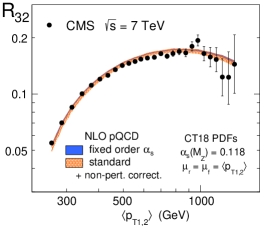
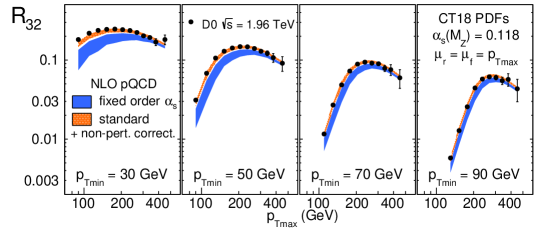
Figure 36: The multijet cross section ratio $R_{3/2}$, measured in p-p collisions at $\sqrt{s}=7$ TeV as a function of $\langle p_{\mathrm{T}1,2}\rangle$ in the CMS experiment CMS:2013vbb and in p-$\bar{\rm p}$ collisions at $\sqrt{s}=1.96$ TeV as a function of $p_{\mathrm{T}}^{\mathrm{max}}$ in the D0 experiment D0:2012dcq . Two sets of pQCD predictions, corrected for non-perturbative contributions, are compared to the data: the fixed-order results for $R_{3/2}$, and the results from the “standard” approach, computed from the ratio of the fixed-order results for the two cross sections. The shaded areas represent the ranges of the scale dependencies of the calculations.

The CMS Collaboration has measured the ratio of the inclusive three-jet and two-jet cross sections, $R_{3/2}$, for jets with $p_{\mathrm{T}}>150\,$GeV and rapidities of $|y|<2.5$ CMS:2013vbb . The results are published as a function of the average transverse momentum of the two leading jets in the event, $\langle p_{\mathrm{T}1,2}\rangle$, over the range $0.42<\langle p_{\mathrm{T}1,2}\rangle<1.39$ TeV, as displayed in Fig. 36 (left). Another measurement of the ratio $R_{3/2}$ was made by the D0 Collaboration for jets with rapidities $|y|<2.4$ and for various lower jet $p_{\mathrm{T}}$ requirements, $p_{\mathrm{T}}^{\mathrm{min}}$. The results are published as a function of the leading jet $p_{\mathrm{T}}$, $p_{\mathrm{T}}^{\mathrm{max}}$, over the range $80<p_{\mathrm{T}}^{\mathrm{max}}<500\,$GeV and for four $p_{\mathrm{T}}^{\mathrm{min}}$ choices from 30 to 90 GeV, as displayed in Fig. 36 (right). The results of the fixed-order and “standard” calculations for the CMS and D0 measurements are compared to the data, with their error bands representing the range of their respective scale dependences. For the CMS results, both methods results are in agreement, and both describe the data equally well. For the D0 data, the fixed-order calculation predicts lower values everywhere and the scale uncertainty bands of the two calculations do either not, or hardly, overlap. Only towards larger $p_{\mathrm{T}}^{\mathrm{min}}$ and larger $p_{\mathrm{T}}^{\mathrm{max}}$, the uncertainty bands get closer.

The D0 Collaboration also published measurements of a new quantity, $R_{\Delta R}$ D0:2012xif which also probes the ratio of three-jet and two-jet production. Starting point is an inclusive jet sample (which probes the two-jet production process). The presence of a neighboring jet with $\Delta R<\pi$ is a sign of an event topology with three or more jets. The fraction of all inclusive jets with a neighboring jet, $R_{\Delta R}$, is therefore also a three- over two-jet cross section ratio. The quantity $R_{\Delta R}$ was measured for different $p_{T}$ requirements, $p_{T\rm min}^{\rm nbr}$, and different angular separations, $\Delta R$, for the neighboring jets, as a function of inclusive jet $p_{T}$ from 50 to 450 GeV. The results of the fixed-order and the “standard” calculations for $R_{\Delta R}$ are compared to the data in Figure 37 (right). In almost all of the phase space the conclusions mirror those for the theoretical description of the CMS $R_{3/2}$ data in Figure 36 (left): The fixed-order pQCD predictions agree with those from the “standard” method, and both give a good description of all data with $p_{T\rm min}^{\rm nbr}\geq 50\,$GeV. Only in the softer regime, for $p_{T\rm min}^{\rm nbr}=30\,$GeV at smaller $p_{T}$, they slightly underestimate the experimental measurement results.

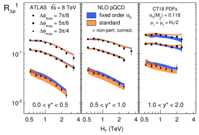
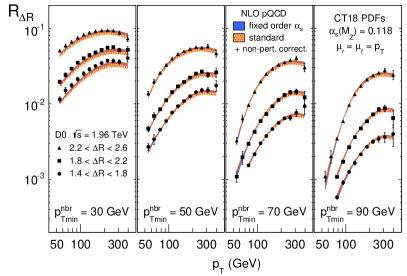
Figure 37: The multijet cross section ratio $R_{\Delta\phi}$, measured in p-p collisions at $\sqrt{s}=8$ TeV in the ATLAS experiment ATLAS:2018sjf (left) as a function of $H_{\mathrm{T}}$, in three regions of $y^{*}$ and for three values of $\Delta\phi_{\rm max}$, and the multijet cross section ratio $R_{\Delta R}$, measured in p-$\bar{\rm p}$ collisions at $\sqrt{s}=1.96$ TeV in the D0 experiment D0:2012xif (right) as a function of $p_{\mathrm{T}}$, in four values of $p_{T\rm min}^{\rm nbr}$ and in three regions of $\Delta R$. Two sets of pQCD predictions, corrected for non-perturbative contributions, are compared to the data: the fixed-order results for $R_{\Delta\phi}$ and $R_{\Delta R}$, and the results from the “standard” approach, computed from the ratio of the fixed-order results for the two cross sections. The shaded areas represent the ranges of the scale dependencies of the calculations.

The measurements of the multijet cross section ratio $R_{\Delta\phi}$ by the D0 and ATLAS Collaborations D0:2012dqa ; ATLAS:2018sjf probe the azimuthal decorrelations of the two leading $p_{T}$ jets in an event, and both analyses follow the recommendations from the original proposal Wobisch:2012au . The ATLAS result is shown in Figure 37 (left). The D0 result is shown in Ref. Sawyer:2021bzn . Both measurements are performed in the same three rapidity regions, $y^{*}$, and for the same azimuthal decorrelation requirements, $\Delta\phi_{\rm max}$. The ATLAS (D0) data are presented as a function of the scalar $p_{T}$ sum of all jets in an event, $H_{T}$, over the range 0.46–4 TeV (180–900 GeV). The degree of agreement between the NLO pQCD predictions from the fixed-order and the “standard” calculations and how they describe the data is pretty much the same for the ATLAS and D0 data sets. In different $y^{*}$ and $\Delta\phi_{\rm max}$ regions, however, the two calculations exhibit a rather different behavior. For $0.<y^{*}<1.$ and $\Delta\phi_{\rm max}=7\pi/8$ and $5\pi/6$, both calculations agree very well, exhibit a relatively small scale dependence, and both describe the data. At $\Delta\phi_{\rm max}=3\pi/4$, the two predictions start to deviate from each other, and in some cases their larger scale uncertainty bands have only a small overlap. The data are described by both predictions. At $1<y^{*}<2$, for $\Delta\phi_{\rm max}=7\pi/8$ and $5\pi/6$, the two predictions have a different $H_{T}$ dependence and disagree at high $H_{T}$. In these regions, the fixed-order calculation gives a better description of the overall $H_{T}$ shape for both data sets.

The results from these comparisons can be summarized as follows: In all cases where the results from the two methods agree with each other (as seen for the CMS $R_{3/2}$, the D0 $R_{\Delta R}$, and some regions of the ATLAS and D0 $R_{\Delta\phi}$ measurements), they also both describe the data. In all cases where the two methods disagree (meaning that their scale uncertainty bands do not overlap, as seen for the D0 $R_{3/2}$ data and the high $H_{T}$ tails in some of the ATLAS and D0 $R_{\Delta\phi}$ data at $y^{*}>1$), one of them (but not always the same) is describing the data. In some intermediate cases, where the scale uncertainty bands from the two methods have little overlap (as for the ATLAS and D0 $R_{\Delta\phi}$ data with $\Delta\phi_{\rm max}=3\pi/4$), both predictions are somehow consistent with the data.

It has to be noted that the “fixed-order” and “standard” method both stand on the same footing. In any given order pQCD, the results from both methods are equally valid representations of the perturbative expansion, and they only differ in higher-order terms. Therefore their discrepancy should be regarded as a genuine uncertainty of a fixed-order calculation, in addition to the scale dependence (since the latter does not always cover the spread of the two methods). The central value can be chosen from either method; there is no fundamental argument, to pick one over the other, and the choice may depend on the specific goal. In $\alpha_{S}$ determinations, where one assumes that the pQCD predictions are able to describe the data, one should possibly pick the method that gives a better description of the data. The proposed treatment of the spread of the two methods as additional uncertainty will provide more realistic estimates of theoretical uncertainties in future $\alpha_{S}$ determinations and other phenomenological studies. A small spread of the two methods can also be a criterion for identifying robust measurable quantities for which the theoretical approximations are more reliable.

6 Energy range for the RGE test and PDF sensitivity in $\alpha_{S}$ evaluations from jet cross section ratios

A series of determinations of $\alpha_{S}$ are performed at the LHC e.g. using jet-based observables, which include the three-jet mass CMS:2014mna , $R_{32}$ ATLAS:2013lla ; CMS:2013vbb ; CMS:2017tvp , transverse energy-energy correlations (TEECs) ATLAS:2017qir and $R_{\Delta\phi}$ ATLAS:2018sjf . We discuss the relevant energy range on which running of the coupling, determined by the renormalisation group equation (RGE), is probed through jet cross-section ratio and event shape observables at hadron colliders, as well as the PDF sensitivity in the corresponding $\alpha_{S}$ evaluations. This contribution is based mainly on remarks made in Refs. Gehrmann:2021qex ; Bogdan_ScalesWorksop_2017 .

For fixed incoming parton kinematics, constructing the ratios between the cross sections for three-jet and two-jet final states can reduce the PDF dependence. At the same time, the resulting $R_{32}$ ratio is still sensitive to $\alpha_{S}$ ATLAS:2013lla ; CMS:2013vbb . The angular decorrelation observable $R_{\Delta\phi}$ in two-jet final states is defined as the ratio between the cross section of events with an azimuthal angular separation below some upper limit and respectively the inclusive dijet cross section. It also allows to probe three-parton final state kinematics and has been used for an $\alpha_{S}$ evaluation ATLAS:2018sjf .

TEECs are event shape variables computed as energy-weighted angular distributions of all individual object pairs in the event. Similarly to e.g. the case of the inclusive jet cross section, a TEEC distribution receives multiple contributions from each event. Since analytical predictions for their distributions can be computed from first principles Dixon:2019uzg , probing hence fundamental symmetries of QCD, the TEECs are particularly attractive observables. The TEECs and the associated asymmetries (ATEEC) were measured by ATLAS and used for a determination of $\alpha_{S}$ ATLAS:2017qir . It is interesting to note that in this study the theoretical prediction is also provided by a three-jet to two-jet cross-section ratio evaluated using NLOJET++ Nagy:2001fj ; Nagy:2003tz , complemented by nonperturbative corrections based on PYTHIA8 Sjostrand:2007gs and HERWIG++ Gieseke:2012ft .

The choice of the scale used in the theoretical calculations for observables like $R_{32}$, $R_{\Delta\phi}$ and (A)TEECs is often based on event-level quantities. Typical examples are the average transverse momentum of the two leading jets CMS:2013vbb ; CMS:2017tvp ; ATLAS:2017qir , the transverse momentum of the leading jet ATLAS:2013lla or half of the scalar sum of the transverse momenta of all the selected jets in the event ATLAS:2018sjf . The evaluated $\alpha_{S}$ values are typically displayed as a function of this same scale, reaching values up to a few TeV (see e.g. Ref. Zyla:2020zbs ). However, we note that the sensitivity to $\alpha_{S}$ for such observables is actually directly related to the probability for emission of extra radiation (yielding a third or higher order jet). This implies that these $\alpha_{S}$ determinations probe the prediction of the renormalisation group equation in QCD at energy scales related to the transverse momentum of the third jet ($p_{\mathrm{T3}}$), rather than to the event-level quantities above. It is to be noted that the typical values for $p_{\mathrm{T3}}$ are indeed significantly lower than the scale based on such event-level quantities. Indeed, in the case of the (A)TEEC studies at 8 TeV ATLAS:2017qir , if the average scales used in the theoretical calculations range between $412$ and $810$ GeV (depending on the bin), the corresponding average $p_{\mathrm{T3}}$ values are between $169$ and $215$ GeV.

It is desirable to achieve consistency between scale used for theory calculation and the scale at which the RGE test is claimed, while taking into account the remarks above. The MiNLO procedure Hamilton:2012np may indeed provide a way forward towards this goal.

The $\alpha_{S}$ determinations from ratios of three-parton-like over two-parton-like final states (i.e. from observables like $R_{32}$, $R_{\Delta\phi}$, (A)TEEC) are impacted by residual PDF uncertainties that have been quantified in the corresponding experimental studies CMS:2014mna ; CMS:2013vbb ; ATLAS:2013lla ; CMS:2017tvp ; ATLAS:2018sjf ; ATLAS:2017qir . Contrary to what one may have initially expected, the PDF uncertainties (originating from the PDF eigenvectors/replicas, as well as from the differences among various PDF sets) are found to be nonnegligible, being typically larger than the combined experimental uncertainties, but smaller than the NLO scale uncertainty (see Table 11). Furthermore, in cases where direct comparisons are possible, it can be noted that the $\alpha_{S}$ determinations from ratio observables can have even larger PDF uncertainties compared to the corresponding absolute cross sections.

Table 11: $\alpha_{S}(m^{2}_{\mathrm{Z}})$ values obtained from various observables are indicated, together with the corresponding uncertainties. The uncertainty components from various sources (experimental, from PDF eigenvectors/replicas, nonperturbative NP, scale variations) or their quadratic sum are displayed, as well as the range of values obtained for various PDF sets. See the corresponding references for any details, in particular for the ensemble of PDF sets considered in each study.

Observable [Ref.]	$\alpha_{S}(m^{2}_{\mathrm{Z}})$	Range PDF variations
$R_{32}$ ATLAS:2013lla	$0.111\pm 0.006\,\mathrm{(exp)}^{+0.016}_{-0.003}\,\mathrm{(PDF,NP,scale)}$	$0.109-0.116$
$R_{32}$ CMS:2013vbb	$0.1148\pm 0.0014\,\mathrm{(exp)}\pm 0.0018\,\mathrm{(PDF)}\pm 0.0050\,\mathrm{(theory)}$	$0.1135-0.1148$
$3$-jet mass CMS:2014mna	$0.1171\pm 0.0013\,\mathrm{(exp)}\pm 0.0024\,\mathrm{(PDF)}\pm 0.0008\,\mathrm{(NP)}^{+0.0069}_{-0.0040}\,\mathrm{(scale)}$	$0.1143-0.1183$
$2$-jets CMS:2017tvp	$0.1159\pm 0.0025\,\mathrm{(exp,PDF,NP)}$	$0.1159-0.1183$
$3$-jets CMS:2017tvp	$0.1161\pm 0.0021\,\mathrm{(exp,PDF,NP)}$	$0.1159-0.1179$
$2$- & 3-jets CMS:2017tvp	$0.1161\pm 0.0021\,\mathrm{(exp,PDF,NP)}$	$0.1161-0.1188$
$R_{32}$ CMS:2017tvp	$0.1150\pm 0.0010\,\mathrm{(exp)}\pm 0.0013\,\mathrm{(PDF)}\pm 0.0015\,\mathrm{(NP)}^{+0.0050}_{-0.0000}\,\mathrm{(scale)}$	$0.1139-0.1184$
TEEC ATLAS:2017qir	$0.1162\pm 0.0011\,\mathrm{(exp)}\pm 0.0018\,\mathrm{(PDF)}\pm 0.0003\,\mathrm{(NP)}^{+0.0076}_{-0.0061}\,\mathrm{(scale)}$	$0.1151-0.1177$
ATEEC ATLAS:2017qir	$0.1196\pm 0.0013\,\mathrm{(exp)}\pm 0.0017\,\mathrm{(PDF)}\pm 0.0004\,\mathrm{(NP)}^{+0.0061}_{-0.0013}\,\mathrm{(scale)}$	$0.1185-0.1206$
$R_{\Delta\phi}$ ATLAS:2018sjf	$0.1127^{+0.0019}_{-0.0018}\,\mathrm{(exp)}\pm 0.0006\,\mathrm{(PDF)}^{+0.0003}_{-0.0001}\,\mathrm{(NP)}^{+0.0052}_{-0.0019}\,\mathrm{(scale)}$	$0.1127-0.1156$

Actually, these features reflect the fact that the three-parton and two-parton processes that are used to define the respective cross section ratios have different composition of partonic initial states (see also contribution by B.M. in Ref. Proceedings:2015eho ). Indeed, the probability of extra radiation (which is what makes these observables nontrivial) is correlated, trough the relevant matrix elements, to the type of partons in the initial state. Furthermore, both the $\alpha_{S}$ and PDF sensitivities of the observables are reduced when taking ratios. Both aspects are relevant for the corresponding evaluations of $\alpha_{S}$, hence the presence of two competing effects resulting in residual PDF uncertainties. This residual PDF sensitivity is especially relevant in phase-space regions where PDFs are not strongly constrained. It can hence be related to the slopes observed in some comparisons of the energy dependence for the extracted $\alpha_{S}$ values, with the corresponding RGE predictions (see e.g. Refs. ATLAS:2017qir ; ATLAS:2018sjf ).

Up to now, the precision of the $\alpha_{S}$ determinations from three-jet-type observables has been limited by the NLO QCD theory uncertainty. This limitation will be overcome due to the NNLO corrections to three-jet production computed recently Czakon:2021mjy , which will allow to perform precision QCD studies with these observables. On the timescale of the FCC projects FCC:2018evy , even more progress on the theoretical predictions for these observables is desirable, allowing to further enhance the precision of these $\alpha_{S}$ evaluations.

7 New results on $\alpha_{S}$ and PDFs: QCD and SMEFT interpretation with inclusive jets at $\sqrt{s}$=13 TeV

Jet production in proton-proton collisions is instrumental for the extraction of the strong coupling constant $\alpha_{S}$ and the parton distribution functions (PDFs). Furthermore, it is sensitive to the presence of physics beyond the standard model (BSM). In the following, the most recent QCD analysis CMS:2021yzl of the inclusive jet cross sections in p-p collisions at the LHC at a center-of-mass energy of 13 TeV is discussed. The data is collected by the CMS Collaboration. The jets are reconstructed using the anti-$k_{T}$ algorithm with the distance parameter $R=0.4$ and $R=0.7$ and the cross sections are measured double-differentially as a function of the individual jet $p_{\mathrm{T}}$ and the absolute rapidity $|y|$. The measurements using $R=0.7$ are used in the QCD analysis and correspond to an integrated luminosity of 33.5 $\mathrm{fb}^{-1}$.

In the QCD analysis, the jet cross sections measured for $R=0.7$ are used, together with the HERA combinedAbramowicz:2015mha inclusive charged- and neutral-current deep inelastic scattering (DIS) cross sections. The fit is performed at NLO and NNLO. In the NLO version of the analysis, together with DIS and CMS jet measurements, the normalized triple-differential cross section of top quark-antiquark ($t\bar{t}$) production measured Sirunyan:2019zvx by the CMS collaboration, are utilized. In the NNLO (NLO) versions of the analysis, the PDFs, the value of $\alpha_{S}(m_{Z})$ (and the value of the top quark pole mass) are determined simultaneously.

Furthermore, an alternative SMEFT analysis is performed at NLO, where the cross section for the inclusive jet production is extended to include the effective contributions of 4-quark contact interactions (CI), exploring three different CI models. In this version of the analysis, the relevant Wilson coefficient is fitted simultaneously with the PDFs and SM parameters, avoiding the possibility of absorbing new physics in the PDF fit. No primary assumptions on the values of the QCD parameters are applied, such that constraints on the SM and BSM parameters are obtained simultaneously, mitigating their possible bias.

The fixed-order QCD predictions for inclusive jet production in p-p collisions are available at NLO and NNLO, obtained with NLOJet++ Nagy:2001fj ; Nagy:2003tz and NNLOJET (rev5918) Currie:2016bfm ; Currie:2018xkj ; Gehrmann:2018szu , respectively, with the NLO calculations implemented in FastNLO Britzger:2012bs . The NLO cross-section is improved to NLO+NLL by using corrections computed using the NLL-Jet calculation, provided by the authors of Ref. Liu:2018ktv , and the MEKS Gao:2012he code. Electroweak and nonperturbative corrections are applied, and their details are given in CMS:2021yzl . The factorisation scale $\mu_{f}$ and renormalisation scale $\mu_{r}$ are set to the individual jet $p_{\mathrm{T}}$ for the inclusive jet cross section, and to the four-momentum transfer $Q$ for the DIS data. In the theory predictions at NLO for the used $t\bar{t}$ production measurements, $\mu_{r}$ and $\mu_{f}$ are set to half the sum of the transverse masses of the partons, following Ref. Sirunyan:2019zvx . The QCD analysis is performed using the xFitter QCD analysis framework Alekhin:2014irh ; Bertone:2017tig with an interface to CIJET Gao:2012qpa ; Gao:2013kp for SMEFT predictions, which are available at NLO.

To illustrate the impact of the 13 TeV data on a global PDF, the profiling procedure Paukkunen:2014zia ; Schmidt:2018hvu ; HERAFitterdevelopersTeam:2015cre is used. The CT14 Dulat:2015mca sets at NLO or NNLO, where appropriate, are chosen. Both the $t\bar{t}$ and jet cross sections are observed to improve the precision of the gluon PDF significantly, as illustrated in Fig. 38 Profiling of the non-PDF parameters, such as the value of $\alpha_{S}(m^{2}_{\mathrm{Z}})$, $m_{t}^{\text{pole}}$ and of the Wilson coefficients of the CI is also performed and the results are summarized in Ref. CMS:2021yzl . The disadvantage of the profiling approach is that the simultaneous extraction of the PDFs and non-PDF parameters is currently not available.

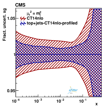
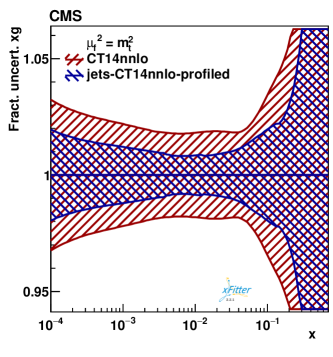
Figure 38: Fractional uncertainties in the gluon distribution, shown as functions of $x$ for the scale $\mu_{f}$ set to the top quark mass. The profiling is performed at NLO with CT14nlo PDF (left) and at NNLO with CT14nnlo, by using the CMS inclusive jet cross section at $\sqrt{s}=13$ TeV. The original uncertainty (red) and the profiled result (blue) uncertainty are shown.

The full QCD analyses, implying the simultaneous fit of the PDF and non-PDF parameters, are performed using SM predictions at NNLO and NLO, or, alternatively, as a SMEFT fit, assuming three SM+CI models. In the SMEFT analyses, the scale of the BSM interaction $\Lambda$ is assumed and the Wilson coefficient $c_{1}$ is a free parameter of the fit, together with the PDF parameters and the values of $\alpha_{S}(m^{2}_{\mathrm{Z}})$ and $m_{t}^{\text{pole}}$. For each of the NLO and NNLO fits, and also for the SMEFT fit, the investigation of the PDF parameterisations is performed independently. The SM fits at NLO and NNLO result in slightly different parameterisations, due to inclusion of the $t\bar{t}$ measurements in the NLO analysis. The SM and SMEFT fits are NLO result in the same solution for the preferred parameterisations.

The uncertainties are estimated following the HERAPDF approach Abramowicz:2015mha , which accounts for the fit, parameterisations and model uncertainties. The Hessian fit uncertainty emerges from the uncertainties in the experimental measurements and is estimated by Hessian method using the tolerance criterion of $\Delta\chi^{2}=1$. The uncertainty is also estimated using the Monte Carlo replica method and the results agree with those obtained by using the Hessian method. The quality of the fit is estimated by $\chi^{2}$ divided by the number of degrees of freedom of $1321/1118$, with somewhat large value driven by the fit to the inclusive DIS data, investigated in detail in Abramowicz:2015mha . The model uncertainties are obtained by varying the assumed non-PDF parameter values such as quark masses, the value of the starting evolution scale, strangeness fraction and the minimum value of $Q^{2}$ of the used DIS data. The theory uncertainties due to missing higher order contributions are obtained by an independent variation of the QCD scales up and down by a factor of 2 (avoiding cases $\mu_{f}/\mu_{f}=4,~{}1/4$). For each of the independent scale choices, the QCD analysis is performed and the difference of the resulting parameters to those obtained for the central scale choice is taken as an uncertainty, which is treated as a model uncertainty. The parameterisations uncertainty arises from adding and removing additional parameters in the PDF parameterisations, one at a time, and constructing a maximum-difference envelope. The total uncertainty in the PDFs is obtained by adding the fit and the model uncertainties in quadrature, while the parameterisations uncertainty is added linearly. To illustrate the improvement in the PDF uncertainty by adding the CMS jet measurements at 13 TeV, the NNLO fit is also performed using only DIS data. A significant improvement in the uncertainty, in particular for the gluon distribution is observed, as shown in Fig. 39. In the same figure, also individual contributions of model, parameterisations and fit uncertainties are shown.

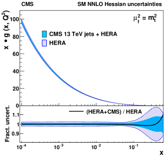
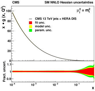
Figure 39: Total (left) and individual (right) fractional uncertainties in the gluon distributions resulting form the NNLO fit, shown as functions of $x$ at the scale $mu_{f}$ of the top quark mass. The filled (hatched) band represents the results of the fit using HERA DIS and the CMS inclusive jet cross section together (using the HERA DIS data only). The line corresponds to the ratio of the central PDF values of the two variants of the fit.

In the SM fit at NNLO, the strong coupling constant $\alpha_{S}(m^{2}_{\mathrm{Z}})$ is obtained simultaneously with the PDFs and results in

$$\alpha_{S}(m^{2}_{\mathrm{Z}})=0.1170\pm 0.0014\,\mathrm{(fit)}\pm 0.0007\,\mathrm{(model)}\pm 0.0008\,\mathrm{(scale)}\pm 0.0001\,\mathrm{(param)},$$ (157)

which agrees with the previous extractions of the strong coupling constant at NNLO at hadron colliders Andreev:2017vxu ; Sirunyan:2018goh , of which it has best precision.

In the SMEFT analysis, the SM Lagrangian is extended with effective operators of dimension 6, introducing vertices with 4 quark legs. The considered operators are colour-singlets and lead to purely left-handed, vector-like and axial vector-like CI models, depending on how the quarks’ handedness may change in the interaction. The operators’ Wilson coefficients are fitted simultaneously with the PDFs, $\alpha_{S}(m^{2}_{\mathrm{Z}})$, and $m_{t}^{\text{pole}}$ at NLO. Independent of the value of $\Lambda$, the strong coupling constant and the top quark mass in these SMEFT fits result to $\alpha_{S}(m^{2}_{\mathrm{Z}})=0.1187\pm 0.0016_{\textrm{(fit)}}\pm 0.0005_{\textrm{(model)}}\pm 0.0023_{\textrm{(scale)}}\pm 0.0018_{\textrm{(param.)}}$, and $m_{t}^{\text{pole}}=170.4\pm 0.6_{\textrm{(fit)}}\pm 0.1_{\textrm{(model)}}\pm 0.1_{\textrm{(scale)}}\pm 0.2_{\textrm{(param.)}}$ GeV. The Wilson coefficients are obtained for different assumed values of $\Lambda$. For illustration, the values of $c_{1}$ are shown for three investigated CI models in Fig. 40 for $\Lambda=50$ TeV.

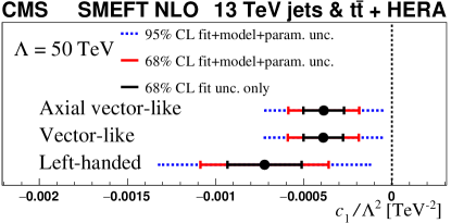
Figure 40: The Wilson coefficients $c_{1}$ obtained in the SMEFT analysis at NLO, divided by $\Lambda^{2}$, for $\Lambda=50$ TeV. The solid (dashed) lines represent the total uncertainty at 68 (95)% CL. The inner (outer) error bars show the fit (total) uncertainty at 68% CL.

To compare to a conventional search for CI, the Wilson coefficients obtained in the SMEFT analysis are translated into unbiased 95% confidence level exclusion limits on $\Lambda$ with $c_{1}=-1$, resulting in the limits of 24 TeV for left-handed, 32 TeV for vector-like, and 31 TeV for axial vector-like CI. The present analysis is the first time such limits are obtained using hadron collider data while following an unbiased search strategy. To compare the PDFs and QCD parameters obtained in the SMEFT fit to respective SM results, the NLO analysis is performed considering only the standard model. The resulting QCD parameters obtained in both variants of the fit, SM and SMEFT, agree well, however the SM results have smaller parametrisation uncertainty. The fit quality of both fits expressed in $\chi^{2}$ divided by number of degrees of freedom results in $1411/1141$ for the SM and $1401/1140$ for SMEFT fits, respectively. The PDFs resulting from the SMEFT fit are shown in Fig. 41 in comparison to the results of the SM fit. Both results agree within the fit uncertainties.

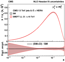
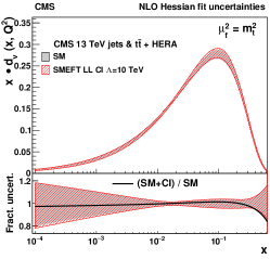
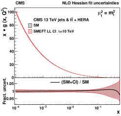
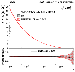
Figure 41: The u-valence (upper left), d-valence (upper right), gluon (lower left), and sea quark (lower right) distributions, shown as functions of $x$ resulting from the fits with and without the CI terms. The SMEFT fit is performed with the left-handed CI model with $\Lambda$ = 10 TeV.

For the future developments, the authors of this measurement and interpretation would appreciate the public availability of the fast-grid techniques for the NNLO prediction of the inclusive jet cross section. Furthermore, the used $t\bar{t}$ data are interpreted at NLO, since the measurements are split into categories according to the presence of an additional jet. In spite of the strong sensitivity of these measurements to the top quark mass, strong coupling constant and to the gluon distribution, these could not be used in the NNLO analysis. A stronger effort in development of the theory calculation for the $t\bar{t}$ production associated with a jet is highly desirable.

The performed SMEFT analysis is only a step towards the global SM+BSM interpretation of the LHC measurements and implies only color-singlet CI contributions. The availability of color-octet contributions and also of the corresponding EFT corrections for the $t\bar{t}$ cross section predictions at NLO, as well as to the other processes, probing the operators of similar structure, would be necessary. Finally, bringing the EFT corrections to the QCD processes to at least NNLO accuracy would be the ultimate goal for the interpretation of the HL-LHC measurements.

8 The strong coupling constant and quark masses

The determination of the strong coupling constant is strongly tied to the determination of other fundamental parameters of the SM and in particular with the quark masses in the QCD Lagrangian. Precise determinations of quark masses typically relies on a comparison of QCD predictions beyond leading-order accuracy with the measurement of experimental observables. These measurements are often sensitive to both the strong coupling constant and the mass value and both parameters should ideally be treated in a simultaneous fit.

Like the strong coupling constant, quark masses are renormalized, scheme-dependent quantities. In the $\overline{\mathrm{MS}}$ scheme the value of the quark mass depends at a given order in perturbation theory on the dimensionful renormalization scale $\mu$. The evolution with this scale, or “running” of the mass, forms a testable prediction of the theory. QCD yields a precise prescription for the scale evolution: given a value for a quark mass at a reference scale, its value at any other scale can be determined using the renormalization group equation (RGE). RGE calculations for the the running quark masses have by now reached the 5-loop (${\cal O}(\alpha_{S}^{5})$) level Vermaseren:1997fq ; Chetyrkin:1997dh ; Baikov:2014qja and software packages such as RunDec Herren:2017osy and REvolver Hoang:2021fhn provide access to state-of-the-art renormalization evolution and scheme conversions.

A large number of measurements over a broad range of energies characterize the evolution of the strong coupling $\alpha_{S}(\mu)$ Zyla:2020zbs . Experimental tests of the running of quark masses have been performed for the charm Gizhko:2017fiu , bottom Abreu:1997ey ; Rodrigo:1997gy ; Abe:1998kr ; Brandenburg:1999nb ; Barate:2000ab ; Abbiendi:2001tw ; Abdallah:2005cv ; Abdallah:2008ac and top quark Sirunyan:2019jyn .

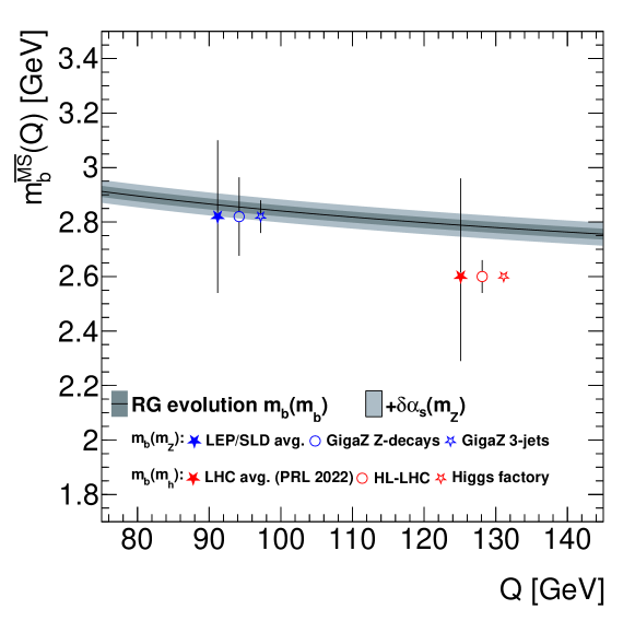
Figure 42: The scale evolution of the bottom quark $\overline{\mathrm{MS}}$ mass. The markers are projections for $m_{b}(m_{\mathrm{Z}})$ from three-jet rates at the Z-pole and for $m_{b}(m_{\mathrm{H}})$ from Higgs boson branching fractions. The prediction of the evolution of the mass is calculated at five-loop precision with REvolver Hoang:2021fhn . The grey error band includes the effect of missing higher orders and the projected parametric uncertainties from $m_{b}(m_{b})$ and $\alpha_{S}$. Note: grey band to be updated with projected $\alpha_{S}$ and $m_{b}(m_{b})$ uncertainty.

Two recent studies revisit the running of the bottom quark mass using Higgs decay measurements at the LHC Aparisi:2021tym and Z-decay rates to bottom quarks at LEP Kluth:2022ucw . The measurement of $m_{b}(m_{\mathrm{H}})$ reaches a competitive precision of 14% with Run-2 measurements. The precision could improve to 2% after the complete LHC programme, including the high-luminosity phase. The method has the potential for a sub-%-level determination at a future electron-positron “Higgs factory”. The three-jet rates in a high-luminosity “GigaZ/TeraZ” Z-pole run at future “Higgs/EW/top factory” electron-positron collider can improve the measurement of $m_{b}(m_{\mathrm{Z}})$ by a factor two ILDnote2020 . The determination of $m_{b}(m_{\mathrm{Z}})$ from the Z $\to b\bar{b}$ decay rate is currently not competitive, but could reach an interesting precision (5%) with a new Z-pole run.

Together, these measurements take the test of the scale evolution of quark masses to a new level of precision Snowmass:bprospects . Figure 42 from Ref. Snowmass:bprospects compares the projections for $m_{b}(m_{\mathrm{Z}})$ and $m_{b}(m_{\mathrm{H}})$ to the current averages and the predicted evolution of the $m_{b}(m_{b})$ world average. The precision of $m_{b}(m_{\mathrm{H}})$ is expected to increase rapidly in Run-3 of the LHC and the HL-LHC programme. A new electron-positron collider operated at the Z-pole and the optimal Higgs-strahlung cross section ($\sim$240–250 GeV) can improve $m_{b}(m_{\mathrm{Z}})$ and $m_{b}(m_{\mathrm{H}})$ further and take tests of the “running” of the bottom quark mass into the precision regime.

The scale evolution of the strong coupling and the quark masses is sensitive to the presence of unknown, massive states that carry colour charge Llorente:2018wup ; Jezabek:1992sq . A combined analysis of the scale evolution of the bottom quark mass and the strong coupling constant is required to consistently treat the impact of the new state on both quantities. A joint fit could possibly include also the charm and top quark masses, that can also be improved with an electron-positron collider Boronat:2019cgt .

With data collected in the next decades at the HL-LHC and a Higgs factory operated at $\sqrt{s}=m_{\mathrm{Z}}$ and $\sqrt{s}\sim$ 250 GeV, the precision of high-scale determinations of the bottom quark mass is expected to increase very significantly, with $m_{b}(m_{\mathrm{H}})$ reaching sub-% precision. A joint analysis of the scale evolution of the strong coupling and the quark masses then provides a powerful and model-independent handle on new coloured states in the mass range between $m_{b}$ and $m_{\mathrm{H}}$.

VIII $\alpha_{S}(m^{2}_{\mathrm{Z}})$ from quarkonium

1 $\alpha_{S}(m^{2}_{\mathrm{Z}})$ from relativistic quarkonium sum rules

One of the classical observables in QCD is the inclusive cross section for $e^{+}e^{-}\to{\rm hadrons}$, which is more conveniently cast in terms of the so-called $R$ ratio defined as

$$R_{q\bar{q}}(s)=\!\frac{3s}{4\pi\alpha^{2}}\sigma_{e^{+}e^{-}\to\,q\bar{q}\,+X}(s)\simeq\dfrac{\sigma_{e^{+}e^{-}\to\,q\bar{q}\,+X}(s)}{\sigma_{e^{+}e^{-}\to\,\mu^{+}\mu^{-}}(s)}\,,$$ (158)

where $\alpha$ is the fine fine-structure constant, $\sqrt{s}$ the center-of-mass energy, and the right-hand side is exact if $\sigma_{e^{+}e^{-}\to\,\mu^{+}\mu^{-}}(s)$ is calculated at tree level for massless muons. Here we are interested in the case of heavy quarks, $q=c,b$.

Integrated moments of $R_{\bar{q}q}(s)$ are particularly suitable for phenomenological studies since, as opposed to local measurements, they have significantly smaller errors and suffer less from residual duality violations, allowing for a direct comparison with computations carried out with partonic degrees of freedom. Furthermore, they can be computed accurately in perturbation theory and receive small nonperturbative corrections, written as an expansion of local operators with increasing dimension. In particular, the inverse moments of $R_{\bar{q}q}(s)$, that we denote $M_{q}^{(n)}$, lead to the following sum rules Shifman:1978bx ; Shifman:1978by

$$M_{q}^{(n)}=\int_{s_{0}}^{\infty}\!\dfrac{{\rm d}s}{s^{n+1}}R_{q\bar{q}}(s)=\dfrac{12\pi^{2}Q_{c}^{2}}{n!}\,\dfrac{{\rm d}^{n}}{{\rm d}s^{n}}\Pi_{q}(s)\Big{|}_{s=0}\,.$$ (159)

On the left-hand side, obtained from experimental data, $s_{0}$ must be below the first $\bar{q}q$ narrow resonance with the same quantum numbers as the photon. On the right-hand side, theoretical moments can be related to derivatives of the heavy-quark vector correlator

$$\!\big{(}g^{\mu\nu}s-p^{\mu}p^{\nu}\big{)}\Pi_{q}(s)=\!-i\!\!\int\!\!{\rm d}x\,e^{i\,p\cdot x}\langle 0|T\,j_{c}^{\mu}(x)j_{c}^{\nu}(0)|0\rangle\,,$$ (160)

evaluated at $s=0$ [ $j_{c}^{\mu}(x)=\bar{q}(x)\gamma^{\mu}q(x)$ ]. The moments are dominated by a short-distance scale given by $\sim m_{q}/n>\Lambda_{\rm QCD}$ (where $m_{q}$ is the quark mass) so restricting $n$ to small values they can be computed in fixed-order QCD and their expansion is known up to $\mathcal{O}(\alpha_{S}^{3})$ for $n\leq 4$ Chetyrkin:1995ii ; Chetyrkin:1996cf ; Boughezal:2006uu ; Czakon:2007qi ; Maier:2007yn ; Chetyrkin:2006xg ; Boughezal:2006px ; Sturm:2008eb ; Maier:2008he ; Maier:2009fz ; Maier:2017ypu . Due to the strong sensitivity of $M_{q}^{(n)}$ to the heavy quark mass, which appears as a prefactor $1/{[2\,\overline{m}_{q}(\mu_{m})]^{2n}}$ in their perturbative expansion, these sum rules have been used for many years to extract $m_{c}$ and $m_{b}$, the masses of the charm and bottom quarks, with very good precision Kuhn:2001dm ; Kuhn:2007vp ; Chetyrkin:2009fv ; Chetyrkin:2010ic ; Chetyrkin:2017lif ; Dehnadi:2011gc ; Dehnadi:2015fra ($\overline{m}_{q}(\mu_{m})$ denotes the $\overline{\rm MS}$ quark mass at scale $\mu_{m}$).

Here we summarize the main results of Refs. Boito:2019pqp ; Boito:2020lyp , where dimensionless ratios of roots of moments $M_{q}^{(n)}$ were considered. Since the ratios of charm-quark moments lead to a more precise determination of the strong coupling (mainly because experimental uncertainties are smaller) we restrict the presentation to the charm-quark moment ratios defined as

$$R_{c}^{V,n}\equiv\frac{\big{(}M_{c}^{(n)}\big{)}^{\frac{1}{n}}}{\big{(}M_{c}^{(n+1)}\big{)}^{\frac{1}{n+1}}}\,.$$ (161)

Ratios of this type were first introduced for the analysis of lattice data for the pseudoscalar correlator Maezawa:2016vgv ; Petreczky:2019ozv (see also the contribution of Petreczky and Weber to this volume, Sec. 4). In the ratios $R_{c}^{V,n}$, the quark-mass dependence from the pre-factor of $M_{c}^{(n)}$ exactly cancels. These dimensionless ratios are suitable for precise $\alpha_{S}$ extractions for the following reasons (some of them already stated):

1. They have a very small residual dependence on the quark mass,

2. are known up to $\mathcal{O}(\alpha_{S}^{3})$ for $1\leq n\leq 3$,

3. contributions from nonperturbative physics are fairly small,

4. they can be determined experimentally from narrow resonance parameters and continuous $R_{\bar{q}q}(s)$ data.

The QCD fixed-order perturbative expansion of the ratios $R_{c}^{V,n}$ reads

$$R^{V,n}_{c}=\sum_{i=0}\bigg{[}\frac{\alpha_{S}(\mu_{\alpha})}{\pi}\bigg{]}^{i}\times\sum_{k=0}^{[i-1]}\sum_{j=0}^{[i-2]}r^{(n)}_{i,j,k}\ln^{j}\biggl{[}\frac{\mu_{m}}{\overline{m}_{c}(\mu_{m})}\biggr{]}\ln^{k}\biggl{[}\frac{\mu_{\alpha}}{\overline{m}_{c}(\mu_{m})}\biggr{]}\,,$$ (162)

where $[i-1]\equiv{\rm Max}(i-1,0)$ and we use $n_{f}=4$ (the $n_{f}$ dependence in $\alpha_{S}$ and the perturbative coefficients will be omitted). The running coupling $\alpha_{S}(\mu_{\alpha})$ and quark mass $\overline{m}_{c}(\mu_{m})$ are expressed in the $\overline{\rm MS}$ scheme and evaluated at the renormalization scales $\mu_{\alpha}$ and $\mu_{m}$, respectively. We do not assume these scales to be the same, as they account for different physics. This leads to a more conservative theory error estimate as argued in Dehnadi:2011gc ; Dehnadi:2015fra . We do avoid, however, large logarithms when varying the scales $\mu_{\alpha}$ and $\mu_{m}$, as discussed below. Note that the leading dependence of the ratios $R^{V,n}_{c}$ on the quark mass is only logarithmic and $\alpha_{S}^{2}$ suppressed. Concretely, for $R_{c}^{V,2}$ at N³LO one finds

$$R_{c}^{V,2}= 1.0449\Bigl{[}1+0.57448\,a_{s}+\bigl{(}0.32576+2.3937\,L_{\alpha}\bigr{)}\,a_{s}^{2}$$ (163)

$$- \bigl{(}2.1093+4.7873L_{m}-6.4009L_{\alpha}-9.9736L_{\alpha}^{2}\bigr{)}\,a_{s}^{3}\,\Bigr{]}\,,$$

with $a_{s}=\alpha_{S}(\mu_{\alpha})/\pi$, $L_{\alpha}=\ln[\,\mu_{\alpha}/\overline{m}_{c}(\mu_{m})\,]$ and $L_{m}=\ln[\,\mu_{m}/\overline{m}_{c}(\mu_{m})\,]$. The total $\alpha_{S}$ corrections are about $12.5\%$ for $R_{c}^{V,1}$, $7.2\%$ for $R_{c}^{V,2}$, and $5.2\%$ for $R_{c}^{V,3}$, which makes these observables rather sensitive to the strong coupling. The dominant nonperturbative correction to these observables stems from the gluon-condensate contribution and is known to NLO. We include it in our analysis, but the numerical impact is small.

We summarize now the determination of the moments $R_{c}^{V,n}$ from experimental data, which consists of three parts: the contribution from the narrow resonances ($J/\psi$ and $\psi^{\prime}$), a contribution from threshold data taken from Refs. Bai:1999pk ; Bai:2001ct ; Ablikim:2004ck ; Ablikim:2006aj ; Ablikim:2006mb ; :2009jsa ; Osterheld:1986hw ; Edwards:1990pc ; Ammar:1997sk ; Besson:1984bd ; :2007qwa ; CroninHennessy:2008yi ; Blinov:1993fw ; Criegee:1981qx ; Abrams:1979cx , and the contribution for $s>10.538$ GeV, where there are no measurements any more, modelled with perturbative QCD (the ‘contiuum contribution’). Since charm threshold data is inclusive in all flavors, one must also perform the subtraction of the $u$, $d$, $s$ background and of the secondary charm production which is not accounted for in theoretical computations. (Small singlet contributions can be neglected Kuhn:2007vp ). It is important to keep the value of $\alpha_{S}$ used in the continuum contribution and the subtraction of the $u$, $d$, $s$ background as a free parameter, otherwise the extraction of the coupling would be biased. For values not too far from the $\alpha_{S}$ world average, the dependence of $R_{c}^{V,n}$ on the strong coupling is linear to an excellent approximation. Parametrizing the results through $\Delta_{\alpha}\equiv\alpha_{S}^{(n_{f}=5)}(m_{Z})-0.1181$ we find

$$R_{c}^{V,1} = (1.770-0.705\,\Delta_{\alpha})\pm 0.017\,,$$ (164)

$$R_{c}^{V,2} = (1.1173-0.1330\,\Delta_{\alpha})\pm 0.0022\,,$$

$$R_{c}^{V,3} = (1.03535-0.04376\,\Delta_{\alpha})\pm 0.00084\,.$$

The above errors are dominated by threshold data and are quite small. This is in part due to positive correlations between the moments $m_{c}^{(n)}$ which produces a partial cancellation of the errors in the ratios.

We extract $\alpha_{S}$ equating the expansions of the type of Eq. (163) with the respective experimental counterparts in Eq. (164) and solving for $\alpha_{S}$ numerically. It is important to carefully and conservatively estimate the theoretical uncertainties arising from the truncation of perturbation theory. In the case of the determination of quark masses, the work of Ref. Dehnadi:2011gc ; Dehnadi:2015fra shows that it is important to vary the two renormalization scales $\mu_{\alpha}$ and $\mu_{m}$ independently. We therefore vary them in the interval $\overline{m}_{c}\leq\mu_{\alpha},\mu_{m}\leq 4~{}{\rm GeV}$ applying the constraint $1/\xi\leq(\mu_{\alpha}/\mu_{m})\leq\xi$ and using $\xi=2$ for our final results. A much less conservative choice, often adopted in related works in the literature, which leads to significantly smaller uncertainties, is to set $\mu_{\alpha}=\mu_{m}$, or equivalently $\xi=1$. We obtain the uncertainties from renormalization scale variation from the spread of values of $\alpha_{S}$ in the $\mu_{m}\times\mu_{\alpha}$ plane, using a grid with 3025 points.

First, we verify the convergence of the extraction of $\alpha_{S}$ order by order in perturbation theory, considering solely the perturbative uncertainty — estimated through the scale variation described above. In Fig. 43 (left), we show that the results display a nice convergence, which indicates that the theory error bars from the truncation of perturbation theory are not underestimated in our analysis. Further light on the perturbative uncertainty can be shed from two-dimensional $\alpha_{S}$ contour plots in the $\mu_{m}\times\mu_{\alpha}$ plane, as shown in Fig. 43 (right) for $R_{c}^{V,2}$. One sees that setting $\mu_{\alpha}=\mu_{m}$ (corresponding to $\xi=1$) the error would be underestimated. Numerically, this choice leads to $\alpha_{S}$ errors obtained from the analysis of $R_{c}^{V,n}$ that are smaller by factors of $3$ ($n=1$), $2$ ($n=2$), and $1.5$ ($n=1$) than those obtained with $\xi=2$.

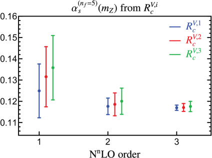
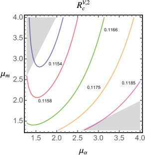
Figure 43: Left: Results for $\alpha_{S}$ obtained from the analysis of $R_{c}^{V,n}$ with $n-=1$, 2, and 3, order by order in perturbation theory. Only truncation errors are shown. Right: Results for $\alpha_{S}$ obtained from $R_{c}^{V,2}$ in the $\mu_{m}\times\mu_{\alpha}$ plane. The shaded region in gray is excluded from the analysis with $\xi=2$ (see text).

We can then extract the final value of $\alpha_{S}$ from our analysis of the charmonium ratios $R_{c}^{V,n}$. Apart from the truncation uncertainty (labelled ‘pt’), discussed in detail above, we include in the final value the experimental error (‘exp’), the incertitude from the residual charm mass dependence (which happens to be negligible), and the nonperturbative error (‘np’, estimated from twice the gluon-condensate contribution). Ratios of moments with lower values of $n$ lead to smaller errors in $\alpha_{S}$ from the truncation of perturbation theory but, on the other hand, have larger experimental uncertainties. In turns out that the optimal determination is obtained from the analysis of $R_{c}^{V,2}$, which gives, after evolving to the Z boson mass scale,

$$\alpha_{S}^{(n_{f}=5)}(m_{Z})=0.1168(15)_{\rm pt}(9)_{\rm exp}(7)_{\rm np}=0.1168(19)\qquad[\,{\rm charm~{}vector~{}current}\,]\,.$$ (165)

This result is fully compatible with the world average Zyla:2020zbs . We remark that by setting $\mu_{\alpha}=\mu_{m}$ the total uncertainty would be reduced to 0.0013, which shows that our error estimate is indeed conservative.

We have applied our method to bottom ratios $R_{b}^{V,n}$ as well, but due to large experimental uncertainties the extracted value for the strong coupling is not competitive. Furthermore, we have reanalysed lattice data on the moments of the pseudoscalar correlator. As opposed to the vector current, the pseudoscalar 0-th moment $m_{c}^{P,0}$, which is scaleless and not sensitive to the charm quark mass, is an observable and therefore a direct comparison to perturbative computations is possible. From higher moments one can construct ratios $R_{c}^{P,n}$ in the same way as displayed in Eq. (161). For either the 0-th moment or the ratios, the exact same program for estimating perturbative errors can be applied, and we find uncertainties that are, in general, larger than what has been quoted in the original lattice articles. In particular, we find that the result in Eq. (165) is slightly more accurate than the extractions that we obtain with our method using lattice results quoted in Refs. HPQCD:2008kxl ; McNeile:2010ji ; Maezawa:2016vgv ; Petreczky:2019ozv ; Nakayama:2016atf .

A slightly more competitive determination can be obtained from a fit to $R_{c}^{V,2}$ and $m_{c}^{P,0}$ (which makes use of the fact that both theoretical and experimental uncertainties for those two observables are uncorrelated), which renders

$$\alpha_{S}^{(n_{f}=5)}(m_{Z})=0.1170\pm(0.0014)_{\rm total}\qquad[\,{\rm lattice\;+\;continuum}\,]\,.$$ (166)

This result can be regarded as a hybrid lattice-continuum determination.

Our ongoing efforts to improve these $\alpha_{S}$ determinations include a more refined treatment of threshold data using an iterative reclustering procedure based on linear splines, in which the new BES-III data BESIII:2021wib on the R-ratio below the charm production threshold has been included. Recent results for the large-order behavior of the perturbative series in the large-$\beta_{0}$ limit of QCD can also guide the design of new moments with reduced perturbative uncertainties, see Ref. Boito:2021wbj . One way of making the bottom sum rules more competitive is taking $n$ large, such that experimental errors virtually vanish. This requires using NRQCD in the theoretical expressions, but the necessary expressions are available since some time already. Finally, as mentioned in the bottomonium section 2, the method explained in the preceding paragraphs should apply equally well to the ratios of bottomonium bound-state masses, which again exhibit experimental errors negligibly small.

Acknowledgments— DB would like to thank the Particle Physics Group of the University of Vienna for hospitality. This work was supported by the FAPESP-USAL SPRINT grant No. 2018/14967-4. DB’s work is supported by the São Paulo Research Foundation (FAPESP) Grants No. 2021/06756-6, the Coordenação de Aperfeiçoamento de Pessoal de Nível Superior – Brasil (CAPES) – Finance Code 001, and by CNPq grant No. 309847/2018-4. VM is supported by the MECD grant PID2019-105439GB-C22, the EU STRONG-2020 project under the program H2020-INFRAIA-2018-1, grant agreement No. 824093 and the COST Action CA16201 PARTICLEFACE.

2 $\alpha_{S}(m^{2}_{\mathrm{Z}})$ determination from bottomonium spectrum

Early attempts to determine $\alpha_{S}$ from quarkonia are based on radiative $\Upsilon(1S)$ decays. Ref. Brambilla:2007cz uses the ratio of the radiative branching ratio over the nonradiative one $\Gamma(\Upsilon(1S)\to X\gamma)/\Gamma(\Upsilon(1S)\to X)$, with $X$ the inclusive set of possible final-state hadrons. The relevant computations can be carried out with partonic degrees of freedom in the final state, and taking into account the charge conjugation of $\Upsilon(1S)$ it reduces to $\Gamma(\Upsilon(1S)\to\gamma gg)/\Gamma(\Upsilon(1S)\to gg)$, where interesting cancellations take place. Hadronic matrix elements also play a role, and need to be computed in the lattice or in the continuum. The theoretical prediction was compared to CLEO data CLEO:2005mdr and the value $\alpha_{S}^{(n_{f}=5)}(m_{\mathrm{Z}})=0.119^{+0.006}_{-0.005}$ was found.

In Ref. Mateu:2017hlz , charmonium and bottomonium spectra were studied within NRQCD, employing the short-distance low-scale scheme for the heavy quark mass known as MSR Hoang:2008yj ; Hoang:2017suc to remove the renormalon inherited from the static potential. Since the bottom and charm quarks are no longer dynamical degrees of freedom they have to be integrated out in the MSR mass as well: this prevents the appearance of large logarithms and the power counting of the theory is not upset. It was shown that for a conservative estimate of perturbative uncertainties the renormalization scales of $\alpha_{S}$ and the MSR mass should be varied independently in a given range determined by the principal quantum number. Furthermore, for a global analysis the scales for the different excited states should be correlated. Even though the main aim of the article was to determine $m_{c}$ and $m_{b}$ from global fits (data for quarkonium masses was taken from the PDG, see Ref. Zyla:2020zbs for updated results), the possibility of obtaining $\alpha_{S}$ from a 2-parameter fit to bottomonium masses was also explored. Since experimental errors on $b\bar{b}$ bound states are tiny, their impact in $\alpha_{S}$ is immaterial. However, the very strong correlation between $m_{b}$ and $\alpha_{S}$ translates into a sizable perturbative uncertainty: $\alpha_{S}^{(n_{f}=5)}(m_{\mathrm{Z}})=0.1178\pm 0.0051$, very similar to that quoted in Ref. Brambilla:2007cz .

A related study Peset:2018ria obtains the strong coupling from a renormalon-free combination of charm and bottom bound-state masses, including $b\bar{c}$, namely $m_{B_{c}}-m_{\eta_{b}}/2-m_{\eta_{c}}/2$, which is also less sensitive to ultrasoft effects. Using the experimental values for the charm and bottom masses as obtained from fits to the masses of $\eta_{c}$ and $\eta_{b}$, respectively, the value $\alpha_{S}^{(n_{f}=5)}(m_{\mathrm{Z}})=0.1195\pm 0.0053$ was obtained, with experimental values for the quarkonium masses taken from the PDG. The uncertainty is very similar to that of Mateu:2017hlz , which opens up the possibility of improving the determination through global fits (determining $m_{c}$, $m_{b}$ and $\alpha_{S}$ simultaneously) to $b\bar{b}$, $c\bar{c}$ and $b\bar{c}$ bound states. Another promising way of obtaining a precise value for the strong coupling is to adapt the strategy of Ref. Boito:2020lyp , see also section 1, to bottomonium. Taking the ratio of bound-states masses with different quantum numbers would cancel most of the heavy quark mass dependence, along with the leading renormalon: the ratios are dimensionless and almost exclusively sensitive to $\alpha_{S}$. Results on this direction will be reported soon.

Acknowledgments— VM is supported by the MECD grant PID2019-105439GB-C22, the EU STRONG-2020 project under the program H2020-INFRAIA-2018-1, grant agreement No. 824093 and the COST Action CA16201 PARTICLEFACE.

IX $\alpha_{S}(m^{2}_{\mathrm{Z}})$ world average

1 Preliminary considerations

We summarize here the current procedure used in the Particle Data Group (PDG) Zyla:2020zbs to obtain the world average value of $\alpha_{S}(m^{2}_{\mathrm{Z}})$ and its uncertainty, and we discuss future prospects for its improvement.

All observables involving the strong interaction depend on the value of the strong coupling constant. This implies that a number of different observables can be used to determine the coupling constant, provided that a suitable theoretical prediction is available for that observable. The following considerations are used to assess if a particular observable is suitable for use in the determination of the strong coupling constant:

• The observable’s sensitivity to $\alpha_{S}$ as compared to the experimental precision. For example, for the ${\rm e^{+}e^{-}}$ cross section to hadrons (e.g. the $R$ ratio), QCD effects are only a small correction, since the perturbative series starts at order $\alpha_{S}^{0}$, but the experimental precision is high. Three-jet production, or event shapes, in ${\rm e^{+}e^{-}}$ annihilation are directly sensitive to $\alpha_{S}$ since they start at order $\alpha_{S}$. Four- and five-jet cross-sections start at $\alpha_{S}^{2}$ and $\alpha_{S}^{3}$ respectively, and hence are very sensitive to $\alpha_{S}$. However, the precision of the measurements deteriorates as the number of jets involved increases.

• The accuracy of the perturbative prediction, or equivalently of the relation between $\alpha_{S}$ and the value of the observable. The minimal requirement is generally considered to be an NLO prediction. The PDG imposes now that at least NNLO accurate predictions be available. In certain cases where phase space restrictions require it, fixed-order predictions are supplemented with resummation. An improved perturbative accuracy is necessary to guarantee that the theoretical uncertainty is assessed in a robust way.

• The size of nonperturbative effects. Sufficiently inclusive quantities, like the ${\rm e^{+}e^{-}}$ cross section to hadrons, have small nonperturbative contributions $\sim{\rm\Lambda}^{4}/Q^{4}$. Other quantities, such as event-shape distributions, typically have contributions $\sim{\rm\Lambda}/Q$. All other aspects being equivalent, observables with smaller nonperturbative corrections are preferable.

• The scale at which the measurement is performed. An uncertainty $\delta$ on a measurement of $\alpha_{S}(Q^{2})$, at a scale $Q$, translates to an uncertainty $\delta^{\prime}=(\alpha_{S}^{2}(m_{\mathrm{Z}}^{2})/\alpha_{S}^{2}(Q^{2}))\cdot\delta$ on $\alpha_{S}(m^{2}_{\mathrm{Z}})$. For example, this enhances the already important impact of precise low-$Q$ measurements, such as from $\tau$ decays, in combinations performed at the $m_{\mathrm{Z}}$ scale.

The PDG determination of $\alpha_{S}$ first separates measurements into a number of different categories, then calculates an average for each category. This average is then used as an input to the world average. The PDG procedure requires four specifications of:

1) the conditions that a determination of $\alpha_{S}$ should fulfill in order be included in the average;

2) the separations of the different extractions of $\alpha_{S}(m^{2}_{\mathrm{Z}})$ into the separate categories;

3) the procedure within each category of the procedure to compute the average and its uncertainty;

4) the manner in which the different subaverages and their uncertainties are combined to determine the final value of $\alpha_{S}(m^{2}_{\mathrm{Z}})$ and its uncertainty.

2 Details of the PDG averaging procedure

In the following, we summarize the procedure adopted in the last edition of the PDG Zyla:2020zbs .

a Criteria for determinations to be included in the world average

In the PDG, the selection of results from which to determine the world average value of $\alpha_{S}(m^{2}_{\mathrm{Z}})$ is restricted to those that are

1. accompanied by reliable estimates of all experimental and theoretical uncertainties;

2. based on the most complete perturbative QCD predictions of at least next-to-next-to leading order (NNLO) accuracy;

3. published in a peer-reviewed journal at the time of writing of the PDG report.

Note that the second condition to some extent follows from the first. In fact, determinations of the strong coupling from observables in ${\rm e^{+}e^{-}}$ involving e.g. five or more jets are very sensitive to $\alpha_{S}$, and could provide additional constraints. However, these observables are currently described only at leading order (LO) or next-to-leading order (NLO), and the determination of the theoretical uncertainty is thus considered not sufficiently robust. It is also important to note that some determinations are included in the PDG, but the uncertainty quoted in the relevant publications is increased by the PDG authors to fulfil the first condition. Similarly, in some cases the central value used in the PDG differs from the one quoted in some publications, but can be extracted from the analysis performed in that work.

b Categories of observables

All observables used in the determination of $\alpha_{S}(m^{2}_{\mathrm{Z}})$ in the PDG exercise are classified in the following categories (Table 12 and Fig. 44):

• “Hadronic $\tau$ decays and low $Q^{2}$ continuum” ($\tau$ decays and low $Q^{2}$):

  Calculations for $\tau$ decays are available at N³LO; there are different approaches to treat the perturbative and nonperturbative contributions, which result in significant differences; the value of $\alpha_{S}$ is determined at the $\tau$ mass;

• “Heavy quarkonia decays and masses” ($Q\overline{Q}$ bound states):

  Calculations are available at NNLO and N³LO;

• “PDF fits” (PDF fits)

  Taken both from global PDF fits and analyses of singlet and non-singlet structure functions; for theory uncertainty, half of the difference between results obtained with NNLO and NLO is added in quadrature;

• “Hadronic final states of ${\rm e^{+}e^{-}}$ annihilations” (${\rm e^{+}e^{-}}$ jets & shapes):

  Taken from measurements at PETRA and LEP; nonperturbative corrections are important and can be estimated either via Monte Carlo simulation or analytic modeling;

• “Observables from hadron-induced collisions” (hadron colliders):

  NNLO calculations for $t\bar{t}$ or jet production at both the LHC and HERA, and Z $+$ jet production at the LHC have allowed measurements for these processes to be used in $\alpha_{S}$ determinations; there is still an open question whether a simultaneous PDF fit has to be carried out to avoid a significant bias;

• “Electroweak precision fit” (electroweak):

  $\alpha_{S}$ determinations are averaged from electroweak fits to data from the Tevatron, LHC, LEP and the SLC; such fits rely on the strict validity of the Standard Model; and

• “Lattice”:

  The average determined by the FLAG group in 2019 from an input of eight determinations was used; the 2021 result came out too late to be included, but the 2021 $\alpha_{S}$ average is very consistent with that of 2019.

Detailed information about which observables are included in the different categories can be found in Ref. Zyla:2020zbs .

c Average and uncertainty in each category

In order to calculate the world average value of $\alpha_{S}(m^{2}_{\mathrm{Z}})$, a preliminary step of pre-averaging results within the each category listed in Sec. b is carried out. For each subfield, except for the “Lattice” category, the unweighted average of all selected results is taken as the pre-average value of $\alpha_{S}(m^{2}_{\mathrm{Z}})$, and the unweighted average of the quoted uncertainties is assigned to be the respective overall error of this pre-average. An unweighted average is used to avoid the situation in which individual measurements, which may be in tension with other measurements and may have underestimated uncertainties, can considerably affect the determination of the strong coupling in a given category. As an example, the determination of $\alpha_{S}(m^{2}_{\mathrm{Z}})$ from ${\rm e^{+}e^{-}}$ jets & shapes currently averages ten determinations and arrives at $\alpha_{S}(m^{2}_{\mathrm{Z}})=0.1171\pm 0.0031$. Since two determinations Abbate:2010xh ; Hoang:2015hka , both based on a similar theoretical framework, arrive at a small value of $\alpha_{S}(m^{2}_{\mathrm{Z}})$ and have a very small uncertainty, if one were to perform a weighted average one would arrive at $\alpha_{S}(m^{2}_{\mathrm{Z}})$ from ${\rm e^{+}e^{-}}$ jets & shapes of $\alpha_{S}(m^{2}_{\mathrm{Z}})=0.1155\pm 0.0006$, which is not compatible with the current world average. This would, in fact, considerably change the world average because of the very small uncertainties. The current procedure is instead robust against $\alpha_{S}(m^{2}_{\mathrm{Z}})$ determinations that are outliers with small uncertainties as compared to the other determinations in the same category. For the “Lattice QCD” (lattice) subfield, we do not perform a pre-averaging step. Instead, we adopt the FLAG2019 average value and uncertainty for this subfield FlavourLatticeAveragingGroup:2019iem . FLAG2019 also requires strict conditions on its own for a determination to be included in their average, which are in line with those used in the PDG. The results of the averages of the categories are given in Table 12. As a follow-up of the workshop the subfields of “$\tau$ decays and low $Q^{2}$” and “$Q\overline{Q}$ bound states” have been updated to account for Ref. Boito:2020xli and Refs. Boito:2019pqp ; Boito:2020lyp , respectively. The world average value does not change.

Table 12: PDG average of the categories of observables [March’22 update of the PDG’21 results]. These are the final input to the world average of $\alpha_{S}(m^{2}_{\mathrm{Z}})$.

category	$\alpha_{S}(m^{2}_{\mathrm{Z}})$	relative $\alpha_{S}(m^{2}_{\mathrm{Z}})$ uncertainty
$\tau$ decays and low $Q^{2}$	$0.1178\pm 0.0019$	1.6%
$Q\overline{Q}$ bound states	$0.1181\pm 0.0037$	3.1%
PDF fits	$0.1162\pm 0.0020$	1.7%
${\rm e^{+}e^{-}}$ jets & shapes	$0.1171\pm 0.0031$	2.6%
electroweak	$0.1208\pm 0.0028$	2.3%
hadron colliders	$0.1165\pm 0.0028$	2.4%
lattice	$0.1182\pm 0.0008$	0.7%
world average (without lattice)	$0.1176\pm 0.0010$	0.9%
world average (with lattice)	$0.1179\pm 0.0009$	0.8%

From the table, it is clear that determinations from different categories are compatible with each other and accordingly can be combined to give rise to a final average.

d Final average

Since the six subfields (excluding lattice) are largely independent of each other, the PDG determines a nonlattice world average value using a standard ‘$\chi^{2}$ averaging’ method. This result in the final average of the six categories of

$$\alpha_{S}(m^{2}_{\mathrm{Z}})=0.1175\pm 0.0010\,,\qquad{\rm(without\,\,lattice)},$$ (167)

which is fully compatible with the lattice determination (Fig. 44). In a last step the PDG performs an unweighted average of the values and uncertainties of $\alpha_{S}(m^{2}_{\mathrm{Z}})$ from the nonlattice result and the lattice result presented in the FLAG2019 report FlavourLatticeAveragingGroup:2019iem , which results in the final average of

$$\alpha_{S}(m^{2}_{\mathrm{Z}})=0.1179\pm 0.0009\,,\qquad{\rm(final\,\,average)}.$$ (168)

Performing a weighted average of all seven categories would instead give rise to $\alpha_{S}(m^{2}_{\mathrm{Z}})=0.1180\pm 0.0006$. The PDG uncertainty is instead more conservative and about 50% larger.

Figure 44: Summary of determinations of $\alpha_{S}(m^{2}_{\mathrm{Z}})$ from seven subfields. The yellow (light shaded) bands and dotted lines indicate the pre-average values of each subfield. The dashed line and blue (dark shaded) band represent the final $\alpha_{S}(m^{2}_{\mathrm{Z}})$ world average [March’22 update of the PDG’21 results Zyla:2020zbs ].

3 Outlook

While the strong coupling remains the least well-known gauge coupling, with an uncertainty of about 1%, it is remarkable that the determinations from all categories agree remarkably well with each other, all within one sigma. Future improvements will be driven by categories which have smallest uncertainties, currently lattice and $\tau$ decays and low $Q^{2}$. The uncertainty quoted in the latter category includes the difference in the extractions that are obtained using contour improved perturbation theory (CIPT) and fixed order perturbation theory (FOPT). Recent arguments suggest that FOPT are to be preferred, see also dedicated discussions on this point in this white paper. If confirmed, this would slightly shift the value of $\alpha_{S}(m^{2}_{\mathrm{Z}})$ in this category to lower values, and would allow one to quote a reduced theoretical uncertainty since this additional source of uncertainty would be completely removed. Further improvements could come from a better understanding of nonperturbative effects. Some progress is also likely to come in the category ${\rm e^{+}e^{-}}$ jets & shapes where the calculation of power corrections in the 3-jet region Luisoni:2020efy ; Caola:2021kzt could have a sizeable impact, and improve fits of the coupling from event shapes. In fact, the region used in the fits are dominated by events with an additional hard emission, therefore the applicability of nonperturbative power corrections computed in the two-jet limit has been questioned and a treatment of these corrections in the three-jet region is certainly more appropriate. The impact of this on $\alpha_{S}(m^{2}_{\mathrm{Z}})$ in this category has still to be assessed. For the hadron collider category it is an open discussion how to deal with correlations between PDF parameters and $\alpha_{S}(m^{2}_{\mathrm{Z}})$ in the cases, where a full fit is not performed simultaneously. In view of many more NNLO results to come we can expect some advances here. Particularly, NNLO for 3-jet production will enable to perform fits of $\alpha_{S}(m^{2}_{\mathrm{Z}})$ from ratios with at least partial cancellation of some uncertainties. Some doubts were raised whether this reduction in uncertainty also holds for the PDF dependence of such ratio predictions. Moreover, for predictions of ratios of cross sections, the central scale definition in numerator and denominator will require more elucidation. Finally, it is important to mention that the last years have seen remarkable advances in the determination of $\alpha_{S}(m^{2}_{\mathrm{Z}})$ from lattice gauge theory, also thanks to the FLAG effort which imposes strict quality criteria for lattice determinations to be included in the FLAG average. This is now the single most precise result of all categories included in the PDG. The challenge is on to still beat it.

X Summary

In this summary section, we provide first an outline of the main points that were the subject of discussions during the $\alpha_{S}(2022)$ workshop, and second we recapitulate the current $\alpha_{S}(m^{2}_{\mathrm{Z}})$ uncertainties of each extraction method as well as the expected experimental and theoretical developments that will help to reduce those in the coming years (and, in some cases, in the longer term of the next generation of collider facilities).

1 Summary of the discussions

During the ECT* workshop, a page on the CERN mattermost service was used to keep notes of the questions and discussions during and after the presentations. Participants were encouraged to join and contribute to the discussions. We provide here a brief summary of the most relevant contributions of the live discussions after the talks, or posted later on the site.

Lattice:

FLAG uses a set of criteria accepted in the community to classify analyses. Only analyses ranking high in all criteria are used to derive the final FLAG determination of the strong coupling. This procedure is very similar to that adopted by the PDG. It was suggested that the FLAG and PDG procedures should be harmonised as much as possible. It was also pointed out that there were updates to individual analyses since the current FLAG 2021 report Aoki:2021kgd was published.

$\tau$ decays:

The discussions covered broadly two areas. The first area concerned the treatment of duality violations (DV) (incomplete asymptotic OPE) terms. One defines moments of the tau spectral function to control and suppress DV terms. However, stronger DV term suppression is correlated with more contributions of condensates leading to a truncated OPE. This was referred to as a kind of “seesaw mechanism” by S. Peris.

The presentation by A. Hoang (Section 4) providing an explanation in terms of renormalon effects of the FOPT vs. CIPT differences in the pQCD predictions, generated considerable interest. The analysis is not yet complete, and further important information would be the value of the gluon condensate normalization. New data would not help directly. The renormalon effects could possibly be studied on the lattice, but this would need a dedicated effort. One would need input from hadronic $\tau$ decay theory to derive observables to be measured on the lattice.

The second topic of discussion involved uncertainties connected with nonperturbative contributions to predictions for the $\tau$ hadronic width that are not directly related to the FOPT vs. CIPT discussion. More and better spectral function data from $\tau$ decays at B-factories or at new ${\rm e^{+}e^{-}}$ colliders, and from ${\rm e^{+}e^{-}}$ annihilation to hadrons at low energies could help to understand and constrain the DV or OPE truncation effects.

Global PDF analyses:

One focus of the discussion in this session was the treatment of theoretical (missing higher-order) uncertainties in the comparison of the predictions with data. The global fit analyses use $\mathcal{O}(1000)$ data points and thus classical $\chi^{2}$-probabilities are hard to interpret, and estimation of parameter uncertainties is difficult. Some authors recommend including the prediction uncertainties in the fits. A critique to this procedure is that this influences and possibly biases the fitted parameter values, including $\alpha_{S}$.

The ATLAS analysis of PDFs (talk by F. Giuli, Section 4) emphasized the importance of a detailed analysis of systematic uncertainties and their correlations in the p-p collision data used in the fit. This was welcomed by global PDF fit groups who would like more detailed information on experimental uncertainties and their correlations.

K. Rabbertz collected a list of open problems in the area of $\alpha_{S}(m^{2}_{\mathrm{Z}})$ determinations from global PDF analyses. This was welcomed in the discussion and could serve as a reference to study and resolve pending and new issues.

${\rm e^{+}e^{-}}$ annihilation to hadronic final states:

The discussions in this area concentrated on the level of understanding of nonperturbative (NP) corrections. The latest results providing a better understanding of power corrections for the $C$-parameter observable (presentation by P. F. Monni and P. Nason, Section 3) were seen as an important step. It was pointed out that a deeper understanding of NP corrections is also needed for other event-shape and for jet-based observables. Other items for improvements were raised such as: NNLO calculations for ${\rm e^{+}e^{-}}\to b\overline{b}g$, NNLL precision parton-shower algorithms and their matching to fixed order predictions and the corresponding retuning of the MC event generators NP parameters (hadronization, colour/flavour/spin correlations etc.). As a potentially useful approach to reduce the NP corrections, groomed observables were discussed. It was stated that by pursuing such an agenda, a better consistency and precision of $\alpha_{S}(m^{2}_{\mathrm{Z}})$ results from ${\rm e^{+}e^{-}}$ annihilation hadronic final states should be possible.

The improved prediction for the $R$-ratio at low energies (A. Nesterenko, Section 1) was discussed as promising, but needs more precise measurements than currently available.

Lepton-hadron colliders:

Analyses at the only so-far operating lepton-hadron collider HERA showed high sensitivity to $\alpha_{S}$ through a large variety of processes with precision measurements available. These include inclusive cross sections, single- or multi-jet production cross sections, event-shape observables, jet-substructure observables, and heavy-flavour cross sections. Unfortunately, most of these measurements were not performed by the HERA experiments using their larger HERA-II data samples, and the only useful published data from HERA-II that achieves 1–2% experimental uncertainties are jet cross sections in neutral-current DIS by H1, and inclusive jet cross section in photoproduction by ZEUS. Since considerable progress on the theory side was made since the HERA times, the H1 and ZEUS collaborations should feel encouraged to continue analyzing their data.

Future e-p experiments provide excellent opportunities for many precision measurements of $\alpha_{S}(m^{2}_{\mathrm{Z}})$. The use of polarized PDFs was highlighted as a novel interesting opportunity at the future EIC. Beyond that, the PDFs from LHeC/FCC-ep will also allow improving many $\alpha_{S}$ analyses done at the HL-LHC.

Hadron colliders:

The analysis presented by D. d’Enterria (Section 2) was discussed for two reasons. First, it was claimed that the use of the MCFM v.8.0 generator to compute inclusive fiducial NNLO cross sections for W and Z bosons could be sensitive to power corrections connected with its subtraction scheme Alekhin:2021xcu . However, in the publication a cross check with a different generator (FEWZ) gave consistent (within few %) results. The second topic was the correlation of $\alpha_{S}(m^{2}_{\mathrm{Z}})$ results from this analysis with results from global PDF analyses, since a few of the more recent PDF global fits also use differential cross section distributions of W- and Z-bosons measured at LHC.

The discussion on this second point moved on to considering merging hadron collider data into global PDF analyses, namely including the inclusive hadron collider cross sections ($t\overline{t}$ and EW bosons at the LHC, and jets at HERA) directly into the global PDF $+\,\alpha_{S}$ fits. The hadron collider extractions use the $\alpha_{S}(m^{2}_{\mathrm{Z}})$ dependence of the public PDF sets to derive the QCD coupling itself, but it was pointed out that this may not converge to the same result as a global PDF $+\,\alpha_{S}$ fit Forte:2020pyp . A complete merging of the “DIS and PDF” and “hadron collider” categories was seen as problematic, since in a global fit with many data sets the impact of a given data set is difficult to quantify. The “Lagrange multiplier” approach of the CT18 group is an advanced example of such studies. One improvement could be to combine a new data set with a PDF fit in order to constrain the PDFs, but report as main result only the obtained $\alpha_{S}$. An example of data sets for individual analysis, possibly together with a PDF fit, are ratios of jet production cross sections. A further problem of global analysis including specific data sets for $\alpha_{S}$ studies is the missing information on correlations of experimental uncertainties between data sets. In addition, the global PDF fits have an intrinsic theory theoretical uncertainty from missing higher-order terms, and any independent $\alpha_{S}(m^{2}_{\mathrm{Z}})$ determination from inclusive cross sections (not used in the fit) provides also a useful cross-check. In any case, since updated PDF (or PDF $+\,\alpha_{S}$) sets are only released every $\sim$5 years, it was clear that keeping the independent measurements of the “hadron collider” $\alpha_{S}$ category of the PDG world-average is appropriate as long as those are not directly incorporated into the global PDF $+\alpha_{S}$ fits.

Other discussions concerned with finding the appropriate choice of renormalisation scale in the pQCD predictions, especially in multiscale observables such as event shapes in p-p collisions (e.g. TEEC, ATEEC, transverse thrust) or (multi)jet production. In addition, the problem of properly determining the correlations between measurements of the different LHC experiments was discussed. Jet production measurements are systematics limited and sensitive to many not easy to control experimental effects. M. Wobisch’s presentation (Section 5) of a different formulation of cross section ratios was seen as another way to estimate theory uncertainties.

The determination of $\alpha_{S}$ from the Z-boson transverse momentum distribution (S. Camarda, Section 3) was seen as a good example for an $\alpha_{S}(m^{2}_{\mathrm{Z}})$ extraction of the hadron collider category since its precision is high (1.3%) and its dependence on PDFs is smaller than other extractions of this subfield. The measurements as well as the theory can further improve in the future.

2 Prospects and wish-lists for high-precision extractions

In Table 13, we summarise the current precision of the seven extraction methods that contribute today to the PDG world average (see Table 12), as well as the expected improvements in the next $\sim$10 years (or in the longer future, in parenthesis) for each one of them. For each category, we list the dominant sources of theoretical and experimental uncertainties that propagate into $\alpha_{S}(m^{2}_{\mathrm{Z}})$ today, and the anticipated progress in the next years (or in the longer term of planned future collider facilities) that will lead to a corresponding reduction of the uncertainties. The last row list the relative uncertainty of the current world-average (0.8%) and of the one expected within the next decade ($\approx$ 0.4%) obtained from taking a weighted average of the individual per-category uncertainties (in parenthesis, we provide the permil precision expected in the longer term from lattice-QCD and/or electroweak fits at a future high-luminosity ${\rm e^{+}e^{-}}$ facility). Of course, the latter result assumes that no new physics impacts any of the extraction methods and, as a matter of fact, significant inconsistency among independent determinations would indicate either a problem in our theoretical/experimental understanding of any given observable, or provide a potential indirect evidence of BSM physics.

Table 13: Summary of current and expected future (within the decade ahead or, in parenthesis, longer time scales) uncertainties in the $\alpha_{S}(m^{2}_{\mathrm{Z}})$ extractions used today to derive the world average. Acronyms and symbols: CIPT=‘contour-improved perturbation theory’, FOPT=‘fixed-order perturbation theory’, NP=‘nonperturbative QCD’, SF=‘structure functions’, PS=‘Monte Carlo parton shower’.

	Relative $\alpha_{S}(m^{2}_{\mathrm{Z}})$ uncertainty
Method	Current	Near (long-term) future
	theory & exp. uncertainties sources	theory & experimental progress
(1) Lattice	$0.7\%$	$\approx\,0.3\%~{}(0.1\%)$
	Finite lattice spacing & stats.	Reduced latt. spacing. Add more observables
	N2,3LO pQCD truncation	Add N3,4LO, active charm (QED effects)
		Higher renorm. scale via step-scaling to more observ.
(2) $\tau$ decays	$1.6\%$	$<1.\%$
	N3LO CIPT vs. FOPT diffs.	Add N4LO terms. Solve CIPT–FOPT diffs.
	Limited $\tau$ spectral data	Improved $\tau$ spectral functions at Belle II
(3) $Q\overline{Q}$ bound states	$3.3\%$	$\approx\,1.5\%$
	N2,3LO pQCD truncation	Add N3,4LO & more $(c\overline{c})$, $(b\overline{b})$ bound states
	$m_{c,b}$ uncertainties	Combined $m_{c,b}+\alpha_{S}$ fits
(4) DIS & PDF fits	$1.7\%$	$\approx\,1\%$ (0.2%)
	N2,(3)LO PDF (SF) fits	N3LO fits. Add new SF fits: $F^{p,d}_{2},\,g_{i}$ (EIC)
	Span of PDF-based results	Better corr. matrices. More PDF data (LHeC/FCC-eh)
(5) ${\rm e^{+}e^{-}}$ jets & evt shapes	$2.6\%$	$\approx\,1.5\%$ ($<1$%)
	NNLO+N(1,2,3)LL truncation	Add N2,3LO+N3LL, power corrections
	Different NP analytical & PS corrs.	Improved NP corrs. via: NNLL PS, grooming
	Limited datasets w/ old detectors	New improved data at B factories (FCC-ee)
(6) Electroweak fits	$2.3\%$	($\approx\,0.1\%$)
	N3LO truncation	N4LO, reduced param. uncerts. ($m_{\mathrm{W,Z}},\,\alpha,$ CKM)
	Small LEP+SLD datasets	Add W boson. Tera-Z, Oku-W datasets (FCC-ee)
(7) Hadron colliders	2.4%	$\approx\,1.5\%$
	NNLO(+NNLL) truncation, PDF uncerts.	N3LO+NNLL (for color-singlets), improved PDFs
	Limited data sets ($t\overline{t}$, W, Z, e-p jets)	Add more datasets: Z $p_{\mathrm{T}}$, p-p jets, $\sigma_{i}/\sigma_{j}$ ratios,…
World average	$0.8\%$	$\approx\,0.4\%$ (0.1%)

Lattice:

The current $\pm 0.7\%$ precision of the lattice-QCD extraction of $\alpha_{S}(m^{2}_{\mathrm{Z}})$ can be reduced by about a factor of two within the next $\sim$10 years. In order to improve the lattice-QCD based determinations of $\alpha_{S}$, it would be important to reach higher renormalization scales. This requires to add more advanced lattice simulations and incorporate improved (higher order) pQCD counterpart calculations. In view of recursive step-scaling strategies, also nonstandard perturbative techniques for selected finite volume renormalization schemes should be developed. Lattice simulations should be run with smaller lattice spacings, allow continuum extrapolation, and include charm quark effects (2+1+1 calculations). Perturbative improvements require calculating N³LO, N⁴LO, and/or N³LL contributions, depending on the process under study. In addition, treatment of QED (and isospin-breaking) effects in the determination of both the scale and the running of $\alpha_{S}$ may be needed in some cases (in particular, when aiming at longer-term 0.1% uncertainties).

$\tau$ decays:

The present $\alpha_{S}(m^{2}_{\mathrm{Z}})$ value of the $\tau$ lepton category has a $\pm 1.6\%$ uncertainty as derived from the pre-averaging of four different determinations. Solving the CIPT vs. FOPT discrepancies, e.g. through the method proposed in Benitez-Rathgeb:2022yqb , is a basic prerequisite to reduce in about a half the current theoretical uncertainty assigned to this extraction method. Although hard to compute, a calculation of the $\mathcal{O}(\alpha_{S}^{5})$ pQCD term (N⁴LO) would be also beneficial, given the sometimes slow convergence of terms with typical weights. On the nonperturbative side, increased data precision would allow more stringent tests of the duality-violation contributions. In particular, more precise 2-pion and 4-pion exclusive-mode $\tau$ data from Belle II would also help to disentangle perturbative and nonperturbative contributions.

$Q\overline{Q}$ bound states:

The $\alpha_{S}(m^{2}_{\mathrm{Z}})$ value derived from quarkonium decays and masses has today a $\pm 3.1\%$ uncertainty from the pre-averaging of six different determinations at NNLO or N³LO accuracy. Improved determinations can be obtained by performing combined fits of $\alpha_{S}$ and charm or bottom quark masses, adding one extra degree of pQCD accuracy to the NNLO predictions, and/or adding more $c\overline{c}$, $b\overline{b}$ bound-states data.

Global PDF analyses:

The current $\alpha_{S}(m^{2}_{\mathrm{Z}})$ value of the parton densities category has a $\pm 1.7\%$ uncertainty as derived from the pre-averaging of six different determinations (two analyses of structure functions, and four from global PDF fits). With complete N³LO predictions for DIS, the residual theoretical uncertainty due to the scale variation and the truncation of the perturbative series will be limited to $\approx$1% in the range of parton kinematics relevant for the current world DIS data and the EIC. Adding new observables, such as e.g. deuteron and spin-dependent structure functions, will also provide new useful constraints. One may hope for progress from analyses at future e-p colliders such as the EIC, LHeC, or FCC-eh. Ultimately, an experimental precision of $\delta\alpha_{S}(m^{2}_{\mathrm{Z}})\sim 0.2\%$ is projected at the LHeC/FCC-eh.

For PDF + $\alpha_{S}$ extractions, future N³LO fits (or, in the shorter term, an improved quantification of the impact of missing higher-order corrections) are required to reach $\approx$1% precision on $\alpha_{S}(m^{2}_{\mathrm{Z}})$. Achieving such a higher degree of pQCD accuracy will likely reduce the present broad span of $\alpha_{S}(m^{2}_{\mathrm{Z}})$ central values among global PDF fits. In addition, the availability of LHC experimental data with more complete information on correlations would improve the global analyses.

${\rm e^{+}e^{-}}$ annihilation to hadronic final states:

The present precision of the $\alpha_{S}(m^{2}_{\mathrm{Z}})$ determination from the ${\rm e^{+}e^{-}}$ category of the PDG world-average is of $\pm 2.6\%$, as obtained by pre-averaging 10 different extractions based on event shapes and/or jet rates. Such a comparatively large uncertainty is driven by the large span among central values derived from measurements where NP corrections have been obtained with Monte Carlo parton showers (PS) or analytically. The former (latter) corrections tend to give larger (smaller) QCD couplings than the world average. The main reduction of this uncertainty will therefore come through an improved convergence between the theoretical (analytical and MC) descriptions of NP effects. First, detailed analytical studies of nonperturbative power corrections exists now for the $C$-parameter that need to be applied to other similar observables, such as thrust, to clarify the current discrepancies. Second, improved parton-shower algorithms (e.g. of the PanXX family) reaching NNLL accuracy are needed, followed by matching to fixed-order (NNLO) predictions plus a full retuning of the hadronization and other final-state parameters (color reconnection, spin correlations,…) of the event generators. In parallel, improved soft-drop grooming techniques should be applied to the ${\rm e^{+}e^{-}}$ data to evaluate their impact in the reduction of NP effects.

Electroweak fits:

The $\alpha_{S}(m^{2}_{\mathrm{Z}})$ uncertainty of the EW category is of $\pm 2.3\%$ and is dominantly driven by the statistical uncertainty in the measurements of the Z-boson pseudoobservables at LEP (the W-boson determination is even much less precise, and features a $\pm 30\%$ uncertainty). Such an $\alpha_{S}(m^{2}_{\mathrm{Z}})$ determination is extremely clean, and can reach the 0.1% precision provided one collects the $10^{12}$ and $10^{8}$ Z- and W-bosons data samples expected at a future high-luminosity ${\rm e^{+}e^{-}}$ collider such as the FCC-ee. To reach such a level of precision will require also to compute missing higher-order pQCD (N⁴LO), EW ${\cal O}(\alpha^{2,3})$, and mixed pQCD+EW $\mathcal{O}(\alpha\alpha_{S}^{2},\,\alpha\alpha_{S}^{3},\,\alpha^{2}\alpha_{S})$ corrections that, today, are negligible compared to the experimental uncertainties.

Hadron colliders:

The QCD coupling derived from the hadron-collider category, obtained from the pre-averaging of 5 different extractions at NNLO accuracy, has a $\pm 2.4\%$ precision today. Theoretical (experimental) uncertainties are driven mostly by the scale and PDF (luminosity) uncertainties. A natural way to reduce the $\alpha_{S}(m^{2}_{\mathrm{Z}})$ uncertainties would be to incorporate N³LO corrections, but this seems realistically feasible in the next years only for color-singlet cross sections, and requires PDFs at the same level of accuracy. A faster way to reduce the current uncertainties by about a half may come from the expected addition of many more upcoming observables (Z $p_{\mathrm{T}}$ peak at $N^{3}$LO, p-p jets and $\sigma_{i}/\sigma_{j}$ ratios at NNLO,…) and/or extended high-precision datasets (integrated luminosity uncertainties at the LHC have been lately reduced to the $\approx$1% level).

a Final wish-list

The determination of the strong coupling has the potential to witness considerable improvements in the decade ahead, with an anticipated reduction in the $\alpha_{S}(m^{2}_{\mathrm{Z}})$ world average uncertainty by a factor of about two (from 0.8% to $\approx$ 0.4%) over this time scale through well-identified experimental and theoretical developments. Such a progress will have an important impact in the theoretical calculations and associated interpretation of upcoming LHC data and in searches for new physics through high-precision SM studies. Such advances will be facilitated by:

• Sufficient dedicated computing resources to generate state-of-the-art samples for lattice QCD analyses. Enough person-power to develop perturbation theory for selected observables in a finite space-time volume, and compute identified higher-order pQCD corrections to match improved lattice QCD samples as necessary basis for $\alpha_{S}$ extractions.

• Beyond lattice-related calculations, person-power is needed for all other important theory efforts. These include the completion of the hadronic $\tau$ decay renormalon analysis, the three-jet power corrections for ${\rm e^{+}e^{-}}$ event shapes and jet algorithms, NNLL accuracy parton shower algorithms and their matching to fixed order, NNLO MCs for complex final states in ${\rm e^{+}e^{-}}$, e-p or p-p scattering, and differential NNLO predictions for HERA and LHC multi-jet observables, among others.

• Incorporation of multiple new precision observables and/or datasets measured at the LHC into NNLO hadron-collider- or PDF- based extractions, with an improved treatment of the experimental correlation uncertainties among measurements, will lead to a visible improvement of the accuracy and precision of the world $\alpha_{S}(m^{2}_{\mathrm{Z}})$ average.

• Measurements of DIS with new high-energy facilities (EIC first and, in the longer term LHeC/FCC-eh) will allow determining PDFs $+\,\alpha_{S}$ over a large phase space covering LHC kinematics. This would resolve PDF-$\alpha_{S}$ ambiguities in hadron-collider analyses, and provide new precision $\alpha_{S}(m^{2}_{\mathrm{Z}})$ determinations. A direct extraction of $\alpha_{S}$ and studies of its energy evolution will also benefit from high-precision PDFs over a large kinematic range.

• Arguably, the only way known to actually reach permil $\alpha_{S}(m^{2}_{\mathrm{Z}})$ uncertainty from purely experimental measurements, without lattice-QCD data simulations, is through the study of hadronic Z (and W) decays. A high-energy lepton collider (Higgs factory, ILC, FCC-ee) with a Giga- or Tera-Z program and low-energy ($\sqrt{s}<m_{Z}$) runs will massively improve ${\rm e^{+}e^{-}}$ determinations of $\alpha_{S}(m^{2}_{\mathrm{Z}})$ via Z- and W-boson hadronic decays, $\tau$ decays, jets rates and event shapes, significantly also improving our understanding of parton showers and nonperturbative effects, and providing accurate tests of the $\alpha_{S}$ evolution.

References

- (1) Particle Data Group Collaboration, P. Zyla et al., “Review of Particle Physics,” PTEP 2020 (2020) 083C01.
- (2) C. Anastasiou, C. Duhr, F. Dulat, E. Furlan, T. Gehrmann, F. Herzog, A. Lazopoulos, and B. Mistlberger, “High precision determination of the gluon fusion Higgs boson cross-section at the LHC,” JHEP 05 (2016) 058, arXiv:1602.00695 [hep-ph].
- (3) A. M. Cooper-Sarkar, M. Czakon, M. A. Lim, A. Mitov, and A. S. Papanastasiou, “Simultaneous extraction of and from LHC differential distributions,” arXiv:2010.04171 [hep-ph].
- (4) A. Blondel, J. Gluza, S. Jadach, P. Janot, and T. Riemann, eds., Theory for the FCC-ee: Report on the 11th FCC-ee Workshop Theory and Experiments, vol. 3/2020 of CERN Yellow Reports: Monographs. CERN, Geneva, May, 2019. arXiv:1905.05078 [hep-ph].
- (5) S. Heinemeyer, S. Jadach, and J. Reuter, “Theory requirements for SM Higgs and EW precision physics at the FCC-ee,” Eur. Phys. J. Plus 136 (2021) 911, arXiv:2106.11802 [hep-ph].
- (6) A. Blondel et al., “Standard model theory for the FCC-ee Tera-Z stage,” in Mini Workshop on Precision EW and QCD Calculations for the FCC Studies : Methods and Techniques, vol. 3/2019 of CERN Yellow Reports: Monographs. CERN, Geneva, 2018. arXiv:1809.01830 [hep-ph].
- (7) A. H. Hoang, “What is the Top Quark Mass?,” Ann. Rev. Nucl. Part. Sci. 70 (2020) 225, arXiv:2004.12915 [hep-ph].
- (8) K. G. Chetyrkin and M. F. Zoller, “Leading QCD-induced four-loop contributions to the -function of the Higgs self-coupling in the SM and vacuum stability,” JHEP 06 (2016) 175, arXiv:1604.00853 [hep-ph].
- (9) J. Llorente and B. P. Nachman, “Limits on new coloured fermions using precision jet data from the Large Hadron Collider,” Nucl. Phys. B 936 (2018) 106, arXiv:1807.00894 [hep-ph].
- (10) S. Bethke et al., eds., Workshop on Precision Measurements of . Sept., 2011. arXiv:1110.0016 [hep-ph].
- (11) D. d’Enterria and P. Z. Skands, eds., Proceedings, High-Precision Measurements from LHC to FCC-ee. CERN, Geneva, Oct., 2015. arXiv:1512.05194 [hep-ph].
- (12) D. d’Enterria and S. Kluth, eds., (2019): Precision measurements of the QCD coupling. PoS ALPHAS2019, July, 2019. arXiv:1907.01435 [hep-ph].
- (13) K. G. Wilson, “Nonlagrangian models of current algebra,” Phys. Rev. 179 (1969) 1499.
- (14) K. Symanzik, “Continuum limit and improved action in lattice theories 1: Principles and theory,” Nucl. Phys. B 226 (1983) 187.
- (15) K. Symanzik, “Continuum limit and improved action in lattice theories 2: O() nonlinear sigma model in perturbation theory,” Nucl. Phys. B 226 (1983) 205.
- (16) J. Komijani, P. Petreczky, and J. H. Weber, “Strong coupling constant and quark masses from lattice QCD,” Prog. Part. Nucl. Phys. 113 (2020) 103788, arXiv:2003.11703 [hep-lat].
- (17) L. Del Debbio and A. Ramos, “Lattice determinations of the strong coupling,” arXiv:2101.04762 [hep-lat].
- (18) Y. Aoki et al., “FLAG Review 2021,” arXiv:2111.09849 [hep-lat].
- (19) K. G. Wilson, “Confinement of quarks,” Phys. Rev. D 10 (1974) 2445.
- (20) G. S. Bali, C. Bauer, and A. Pineda, “Perturbative expansion of the plaquette to in four-dimensional SU(3) gauge theory,” Phys. Rev. D 89 (2014) 054505, arXiv:1401.7999 [hep-ph].
- (21) G. S. Bali, C. Bauer, and A. Pineda, “Model-independent determination of the gluon condensate in four-dimensional SU(3) gauge theory,” Phys. Rev. Lett. 113 (2014) 092001, arXiv:1403.6477 [hep-ph].
- (22) HPQCD Collaboration, Q. Mason, H. D. Trottier, C. T. H. Davies, K. Foley, A. Gray, G. P. Lepage, M. Nobes, and J. Shigemitsu, “Accurate determinations of from realistic lattice QCD,” Phys. Rev. Lett. 95 (2005) 052002, arXiv:hep-lat/0503005.
- (23) HPQCD Collaboration, C. T. H. Davies, K. Hornbostel, I. D. Kendall, G. P. Lepage, C. McNeile, J. Shigemitsu, and H. Trottier, “Update: Accurate determinations of from realistic lattice QCD,” Phys. Rev. D 78 (2008) 114507, arXiv:0807.1687 [hep-lat].
- (24) K. Maltman, D. Leinweber, P. Moran, and A. Sternbeck, “The realistic lattice determination of revisited,” Phys. Rev. D 78 (2008) 114504, arXiv:0807.2020 [hep-lat].
- (25) Flavour Lattice Averaging Group Collaboration, S. Aoki et al., “FLAG Review 2019: Flavour Lattice Averaging Group (FLAG),” Eur. Phys. J. C 80 (2020) 113, arXiv:1902.08191 [hep-lat].
- (26) PACS-CS Collaboration, S. Aoki et al., “Precise determination of the strong coupling constant in = 2+1 lattice QCD with the Schrodinger functional scheme,” JHEP 10 (2009) 053, arXiv:0906.3906 [hep-lat].
- (27) C. McNeile, C. T. H. Davies, E. Follana, K. Hornbostel, and G. P. Lepage, “High-precision and masses, and QCD coupling from current-current correlators in lattice and continuum QCD,” Phys. Rev. D 82 (2010) 034512, arXiv:1004.4285 [hep-lat].
- (28) B. Chakraborty, C. T. H. Davies, B. Galloway, P. Knecht, J. Koponen, G. C. Donald, R. J. Dowdall, G. P. Lepage, and C. McNeile, “High-precision quark masses and QCD coupling from lattice QCD,” Phys. Rev. D 91 (2015) 054508, arXiv:1408.4169 [hep-lat].
- (29) ALPHA Collaboration, M. Bruno, M. Dalla Brida, P. Fritzsch, T. Korzec, A. Ramos, S. Schaefer, H. Simma, S. Sint, and R. Sommer, “QCD Coupling from a Nonperturbative Determination of the Three-Flavor Parameter,” Phys. Rev. Lett. 119 (2017) 102001, arXiv:1706.03821 [hep-lat].
- (30) TUMQCD Collaboration, A. Bazavov, N. Brambilla, X. Garcia i Tormo, P. Petreczky, J. Soto, A. Vairo, and J. H. Weber, “Determination of the QCD coupling from the static energy and the free energy,” Phys. Rev. D 100 (2019) 114511, arXiv:1907.11747 [hep-lat].
- (31) C. Ayala, X. Lobregat, and A. Pineda, “Determination of from an hyperasymptotic approximation to the energy of a static quark-antiquark pair,” JHEP 09 (2020) 016, arXiv:2005.12301 [hep-ph].
- (32) S. Cali, K. Cichy, P. Korcyl, and J. Simeth, “Running coupling constant from position-space current-current correlation functions in three-flavor lattice QCD,” Phys. Rev. Lett. 125 (2020) 242002, arXiv:2003.05781 [hep-lat].
- (33) A. Athenodorou, J. Finkenrath, F. Knechtli, T. Korzec, B. Leder, M. Marinković Krstić, and R. Sommer, “How perturbative are heavy sea quarks?,” Nucl. Phys. B 943 (2019) 114612, arXiv:1809.03383 [hep-lat].
- (34) W. Bernreuther and W. Wetzel, “Decoupling of heavy quarks in the minimal subtraction scheme,” Nucl. Phys. B 197 (1982) 228. [Erratum: Nucl. Phys. B513, 758 (1998)].
- (35) A. G. Grozin, M. Hoeschele, J. Hoff, and M. Steinhauser, “Simultaneous decoupling of bottom and charm quarks,” JHEP 09 (2011) 066, arXiv:1107.5970 [hep-ph].
- (36) K. G. Chetyrkin, J. H. Kühn, and C. Sturm, “QCD decoupling at four loops,” Nucl. Phys. B 744 (2006) 121, arXiv:hep-ph/0512060.
- (37) Y. Schröder and M. Steinhauser, “Four-loop decoupling relations for the strong coupling,” JHEP 01 (2006) 051, arXiv:hep-ph/0512058.
- (38) B. A. Kniehl, A. V. Kotikov, A. I. Onishchenko, and O. L. Veretin, “Strong-coupling constant with flavor thresholds at five loops in the anti-MS scheme,” Phys. Rev. Lett. 97 (2006) 042001, arXiv:hep-ph/0607202.
- (39) M. Gerlach, F. Herren, and M. Steinhauser, “Wilson coefficients for Higgs boson production and decoupling relations to ,” JHEP 11 (2018) 141, arXiv:1809.06787 [hep-ph].
- (40) M. Lüscher, R. Narayanan, P. Weisz, and U. Wolff, “The Schrodinger functional: A Renormalizable probe for nonAbelian gauge theories,” Nucl. Phys. B 384 (1992) 168, arXiv:hep-lat/9207009 [hep-lat].
- (41) S. Weinberg, “New approach to the renormalization group,” Phys. Rev. D 8 (1973) 3497.
- (42) M. Lüscher, P. Weisz, and U. Wolff, “A Numerical method to compute the running coupling in asymptotically free theories,” Nucl. Phys. B 359 (1991) 221.
- (43) N. Husung, A. Nada, and R. Sommer, “Yang Mills short distance potential and perturbation theory,” PoS LATTICE2019 (2020) 263.
- (44) ALPHA Collaboration, M. Dalla Brida, R. Höllwieser, F. Knechtli, T. Korzec, A. Ramos, and R. Sommer, “Non-perturbative renormalization by decoupling,” Phys. Lett. B 807 (2020) 135571, arXiv:1912.06001 [hep-lat].
- (45) M. Dalla Brida, “Past, present, and future of precision determinations of the QCD parameters from lattice QCD,” Eur. Phys. J. A 57 (2021) 66, arXiv:2012.01232 [hep-lat].
- (46) M. Dalla Brida and A. Ramos, “The gradient flow coupling at high-energy and the scale of SU(3) Yang–Mills theory,” Eur. Phys. J. C 79 (2019) 720, arXiv:1905.05147 [hep-lat].
- (47) A. Nada and A. Ramos, “An analysis of systematic effects in finite size scaling studies using the gradient flow,” Eur. Phys. J. C 81 (2021) 1, arXiv:2007.12862 [hep-lat].
- (48) ALPHA Collaboration, M. D. Brida, R. Höllwieser, F. Knechtli, T. Korzec, A. Nada, A. Ramos, S. Sint, and R. Sommer, “Results for from the decoupling strategy,” in 38th International Symposium on Lattice Field Theory. Dec., 2021. arXiv:2112.09623 [hep-lat].
- (49) ALPHA Collaboration, M. Dalla Brida, P. Fritzsch, T. Korzec, A. Ramos, S. Sint, and R. Sommer, “A non-perturbative exploration of the high energy regime in QCD,” Eur. Phys. J. C 78 (2018) 372, arXiv:1803.10230 [hep-lat].
- (50) ALPHA Collaboration, M. Dalla Brida, P. Fritzsch, T. Korzec, A. Ramos, S. Sint, and R. Sommer, “Determination of the QCD parameter and the accuracy of perturbation theory at high energies,” Phys. Rev. Lett. 117 (2016) 182001, arXiv:1604.06193 [hep-ph].
- (51) R. Sommer and U. Wolff, “Non-perturbative computation of the strong coupling constant on the lattice,” Nucl. Part. Phys. Proc. 261 (2015) 155, arXiv:1501.01861 [hep-lat].
- (52) K. Jansen, C. Liu, M. Lüscher, H. Simma, S. Sint, et al., “Nonperturbative renormalization of lattice QCD at all scales,” Phys. Lett. B 372 (1996) 275, hep-lat/9512009.
- (53) ALPHA Collaboration, M. Dalla Brida, P. Fritzsch, T. Korzec, A. Ramos, S. Sint, and R. Sommer, “Slow running of the Gradient Flow coupling from 200 MeV to 4 GeV in QCD,” Phys. Rev. D 95 (2017) 014507, arXiv:1607.06423 [hep-lat].
- (54) S. Weinberg, “Effective gauge theories,” Phys. Lett. B 91 (1980) 51.
- (55) ALPHA Collaboration, M. Bruno, J. Finkenrath, F. Knechtli, B. Leder, and R. Sommer, “Effects of heavy sea quarks at low energies,” Phys. Rev. Lett. 114 (2015) 102001, arXiv:1410.8374 [hep-lat].
- (56) ALPHA Collaboration, F. Knechtli, T. Korzec, B. Leder, and G. Moir, “Power corrections from decoupling of the charm quark,” Phys. Lett. B 774 (2017) 649, arXiv:1706.04982 [hep-lat].
- (57) ALPHA Collaboration, R. Höllwieser, F. Knechtli, and T. Korzec, “Scale setting for QCD,” Eur. Phys. J. C 80 (2020) 349, arXiv:2002.02866 [hep-lat].
- (58) B. Dehnadi, A. H. Hoang, and V. Mateu, “Bottom and Charm Mass Determinations with a Convergence Test,” JHEP 08 (2015) 155, arXiv:1504.07638 [hep-ph].
- (59) D. Boito and V. Mateu, “Precise determination of from relativistic quarkonium sum rules,” JHEP 03 (2020) 094, arXiv:2001.11041 [hep-ph].
- (60) C. Sturm, “Moments of Heavy Quark Current Correlators at Four-Loop Order in Perturbative QCD,” JHEP 09 (2008) 075, arXiv:0805.3358 [hep-ph].
- (61) Y. Kiyo, A. Maier, P. Maierhofer, and P. Marquard, “Reconstruction of heavy quark current correlators at ,” Nucl. Phys. B 823 (2009) 269, arXiv:0907.2120 [hep-ph].
- (62) A. Maier, P. Maierhofer, P. Marquard, and A. V. Smirnov, “Low energy moments of heavy quark current correlators at four loops,” Nucl. Phys. B 824 (2010) 1, arXiv:0907.2117 [hep-ph].
- (63) HPQCD Collaboration, I. Allison et al., “High-Precision Charm-Quark Mass from Current-Current Correlators in Lattice and Continuum QCD,” Phys. Rev. D 78 (2008) 054513, arXiv:0805.2999 [hep-lat].
- (64) Y. Maezawa and P. Petreczky, “Quark masses and strong coupling constant in 2+1 flavor QCD,” Phys. Rev. D 94 (2016) 034507, arXiv:1606.08798 [hep-lat].
- (65) P. Petreczky and J. H. Weber, “Strong coupling constant and heavy quark masses in (2+1)-flavor QCD,” Phys. Rev. D 100 (2019) 034519, arXiv:1901.06424 [hep-lat].
- (66) P. Petreczky and J. H. Weber, “Strong coupling constant from moments of quarkonium correlators revisited,” Eur. Phys. J. C 82 (2022) 64, arXiv:2012.06193 [hep-lat].
- (67) K. Nakayama, B. Fahy, and S. Hashimoto, “Short-distance charmonium correlator on the lattice with Möbius domain-wall fermion and a determination of charm quark mass,” Phys. Rev. D 94 (2016) 054507, arXiv:1606.01002 [hep-lat].
- (68) G. P. Lepage and P. B. Mackenzie, “On the viability of lattice perturbation theory,” Phys. Rev. D 48 (1993) 2250, arXiv:hep-lat/9209022.
- (69) J. H. Weber, “Strong coupling constant and heavy quark masses in (2+1)-flavor QCD,” PoS LATTICE2019 (2020) 101.
- (70) N. Brambilla, A. Pineda, J. Soto, and A. Vairo, “Potential NRQCD: An Effective theory for heavy quarkonium,” Nucl. Phys. B 566 (2000) 275, arXiv:hep-ph/9907240.
- (71) N. Brambilla, A. Pineda, J. Soto, and A. Vairo, “The Infrared behavior of the static potential in perturbative QCD,” Phys. Rev. D 60 (1999) 091502, arXiv:hep-ph/9903355.
- (72) C. Anzai, Y. Kiyo, and Y. Sumino, “Static QCD potential at three-loop order,” Phys. Rev. Lett. 104 (2010) 112003, arXiv:0911.4335 [hep-ph].
- (73) A. V. Smirnov, V. A. Smirnov, and M. Steinhauser, “Three-loop static potential,” Phys. Rev. Lett. 104 (2010) 112002, arXiv:0911.4742 [hep-ph].
- (74) A. Pineda and J. Soto, “The Renormalization group improvement of the QCD static potentials,” Phys. Lett. B 495 (2000) 323, arXiv:hep-ph/0007197.
- (75) N. Brambilla, X. Garcia i Tormo, J. Soto, and A. Vairo, “The Logarithmic contribution to the QCD static energy at N4LO,” Phys. Lett. B 647 (2007) 185, arXiv:hep-ph/0610143.
- (76) N. Brambilla, A. Vairo, X. Garcia i Tormo, and J. Soto, “The QCD static energy at NNNLL,” Phys. Rev. D 80 (2009) 034016, arXiv:0906.1390 [hep-ph].
- (77) T. Appelquist, M. Dine, and I. J. Muzinich, “The Static Potential in Quantum Chromodynamics,” Phys. Lett. B 69 (1977) 231.
- (78) A. Pineda and J. Soto, “Effective field theory for ultrasoft momenta in NRQCD and NRQED,” Nucl. Phys. B Proc. Suppl. 64 (1998) 428, arXiv:hep-ph/9707481.
- (79) A. Bazavov, N. Brambilla, X. Garcia i Tormo, P. Petreczky, J. Soto, and A. Vairo, “Determination of from the QCD static energy,” Phys. Rev. D 86 (2012) 114031, arXiv:1205.6155 [hep-ph].
- (80) S. Necco and R. Sommer, “The N(f) = 0 heavy quark potential from short to intermediate distances,” Nucl. Phys. B 622 (2002) 328, arXiv:hep-lat/0108008.
- (81) A. Pineda, “The Static potential: Lattice versus perturbation theory in a renormalon based approach,” J. Phys. G 29 (2003) 371, arXiv:hep-ph/0208031.
- (82) N. Brambilla, X. Garcia i Tormo, J. Soto, and A. Vairo, “Precision determination of from the QCD static energy,” Phys. Rev. Lett. 105 (2010) 212001, arXiv:1006.2066 [hep-ph]. [Erratum: Phys.Rev.Lett. 108, 269903 (2012)].
- (83) A. Bazavov, N. Brambilla, X. G. Tormo, I, P. Petreczky, J. Soto, and A. Vairo, “Determination of from the QCD static energy: An update,” Phys. Rev. D 90 (2014) 074038, arXiv:1407.8437 [hep-ph]. [Erratum: Phys.Rev.D 101, 119902 (2020)].
- (84) J. H. Weber, A. Bazavov, and P. Petreczky, “Equation of state in (2+1) flavor QCD at high temperatures,” PoS Confinement2018 (2019) 166, arXiv:1811.12902 [hep-lat].
- (85) A. Bazavov, P. Petreczky, and J. H. Weber, “Equation of state in 2+1 flavor QCD at high temperatures,” Phys. Rev. D 97 (2018) 014510, arXiv:1710.05024 [hep-lat].
- (86) S. Steinbeißer, N. Brambilla, R. L. Delgado, A. S. Kronfeld, V. Leino, P. Petreczky, A. Vairo, and J. H. Weber, “The static energy in 2+1+1-flavor QCD,” in 38th International Symposium on Lattice Field Theory. Nov., 2021. arXiv:2111.02288 [hep-lat].
- (87) H. Takaura, T. Kaneko, Y. Kiyo, and Y. Sumino, “Determination of from static QCD potential: OPE with renormalon subtraction and lattice QCD,” JHEP 04 (2019) 155, arXiv:1808.01643 [hep-ph].
- (88) H. Takaura, T. Kaneko, Y. Kiyo, and Y. Sumino, “Determination of from static QCD potential with renormalon subtraction,” Phys. Lett. B 789 (2019) 598, arXiv:1808.01632 [hep-ph].
- (89) HotQCD Collaboration, A. Bazavov et al., “Equation of state in (2+1)-flavor QCD,” Phys. Rev. D 90 (2014) 094503, arXiv:1407.6387 [hep-lat].
- (90) JLQCD Collaboration, T. Kaneko, S. Aoki, G. Cossu, H. Fukaya, S. Hashimoto, and J. Noaki, “Large-scale simulations with chiral symmetry,” PoS LATTICE2013 (2014) 125, arXiv:1311.6941 [hep-lat].
- (91) A. Vairo, “A low-energy determination of at three loops,” EPJ Web Conf. 126 (2016) 02031, arXiv:1512.07571 [hep-ph].
- (92) N. Brambilla, V. Leino, O. Philipsen, C. Reisinger, A. Vairo, and M. Wagner, “Lattice gauge theory computation of the static force,” arXiv:2106.01794 [hep-lat].
- (93) V. Leino, N. Brambilla, J. Mayer-Steudte, and A. Vairo, “The static force from generalized Wilson loops using gradient flow,” EPJ Web Conf. 258 (2022) 04009, arXiv:2111.10212 [hep-lat].
- (94) M. Berwein, N. Brambilla, P. Petreczky, and A. Vairo, “Polyakov loop correlator in perturbation theory,” Phys. Rev. D 96 (2017) 014025, arXiv:1704.07266 [hep-ph]. [Addendum: Phys.Rev.D 101, 099903 (2020)].
- (95) TUMQCD Collaboration, A. Bazavov, N. Brambilla, P. Petreczky, A. Vairo, and J. H. Weber, “Color screening in (2+1)-flavor QCD,” Phys. Rev. D 98 (2018) 054511, arXiv:1804.10600 [hep-lat].
- (96) A. Pich, “Precision physics with inclusive QCD processes,” Prog. Part. Nucl. Phys. 117 (2021) 103846, arXiv:2012.04716 [hep-ph].
- (97) E. Braaten, S. Narison, and A. Pich, “QCD analysis of the tau hadronic width,” Nucl. Phys. B 373 (1992) 581.
- (98) M. A. Shifman, A. I. Vainshtein, and V. I. Zakharov, “QCD and Resonance Physics. Theoretical Foundations,” Nucl. Phys. B 147 (1979) 385.
- (99) P. A. Baikov, K. G. Chetyrkin, and J. H. Kuhn, “Order QCD corrections to and decays,” Phys. Rev. Lett. 101 (2008) 012002, arXiv:0801.1821 [hep-ph].
- (100) F. Le Diberder and A. Pich, “Testing QCD with tau decays,” Phys. Lett. B 289 (1992) 165.
- (101) M. González-Alonso, A. Pich, and A. Rodríguez-Sánchez, “Updated determination of chiral couplings and vacuum condensates from hadronic decay data,” Phys. Rev. D 94 (2016) 014017, arXiv:1602.06112 [hep-ph].
- (102) M. Davier, A. Höcker, B. Malaescu, C.-Z. Yuan, and Z. Zhang, “Update of the ALEPH non-strange spectral functions from hadronic decays,” Eur. Phys. J. C 74 (2014) 2803, arXiv:1312.1501 [hep-ex].
- (103) A. Pich and A. Rodríguez-Sánchez, “Determination of the QCD coupling from ALEPH decay data,” Phys. Rev. D 94 (2016) 034027, arXiv:1605.06830 [hep-ph].
- (104) ALEPH Collaboration, S. Schael et al., “Branching ratios and spectral functions of tau decays: Final ALEPH measurements and physics implications,” Phys. Rept. 421 (2005) 191, arXiv:hep-ex/0506072.
- (105) CLEO Collaboration, T. Coan et al., “Measurement of from tau decays,” Phys. Lett. B 356 (1995) 580.
- (106) OPAL Collaboration, K. Ackerstaff et al., “Measurement of the strong coupling constant and the vector and axial vector spectral functions in hadronic tau decays,” Eur. Phys. J. C 7 (1999) 571, arXiv:hep-ex/9808019.
- (107) A. Pich, “Precision Tau Physics,” Prog. Part. Nucl. Phys. 75 (2014) 41, arXiv:1310.7922 [hep-ph].
- (108) F. Le Diberder and A. Pich, “The perturbative QCD prediction to revisited,” Phys. Lett. B 286 (1992) 147.
- (109) A. A. Pivovarov, “Renormalization group analysis of the tau lepton decay within QCD,” Z. Phys. C 53 (1992) 461, arXiv:hep-ph/0302003 [hep-ph]. [Sov. J. Nucl. Phys.54,676(1991); Yad. Fiz.54,1114(1991)].
- (110) A. Pich and A. Rodríguez-Sánchez, “Updated determination of from tau decays,” Mod. Phys. Lett. A 31 (2016) 1630032, arXiv:1606.07764 [hep-ph].
- (111) A. Pich, “Tau-decay determination of the strong coupling,” SciPost Phys. Proc. 1 (2019) 036, arXiv:1811.10067 [hep-ph].
- (112) C. Ayala, G. Cvetic, and D. Teca, “Using improved Operator Product Expansion in Finite Energy Sum Rules with ALEPH decay data, and determination of pQCD coupling,” arXiv:2112.01992 [hep-ph].
- (113) ALEPH Collaboration, R. Barate et al., “Measurement of the spectral functions of axial - vector hadronic tau decays and determination of ,” Eur. Phys. J. C 4 (1998) 409.
- (114) M. Beneke, “Renormalons,” Phys. Rept. 317 (1999) 1, arXiv:hep-ph/9807443.
- (115) M. Beneke and M. Jamin, “ and the tau hadronic width: fixed-order, contour-improved and higher-order perturbation theory,” JHEP 09 (2008) 044, arXiv:0806.3156 [hep-ph].
- (116) M. Beneke, D. Boito, and M. Jamin, “Perturbative expansion of tau hadronic spectral function moments and extractions,” JHEP 01 (2013) 125, arXiv:1210.8038 [hep-ph].
- (117) A. H. Hoang and C. Regner, “Borel Representation of Hadronic Spectral Function Moments in Contour-Improved Perturbation Theory,” arXiv:2008.00578 [hep-ph].
- (118) A. H. Hoang and C. Regner, “On the Difference between FOPT and CIPT for Hadronic Tau Decays,” Eur. Phys. J. ST 230 (2021) , arXiv:2105.11222 [hep-ph].
- (119) D. Boito, M. Golterman, K. Maltman, S. Peris, M. V. Rodrigues, and W. Schaaf, “Strong coupling from an improved vector isovector spectral function,” Phys. Rev. D 103 (2021) 034028, arXiv:2012.10440 [hep-ph].
- (120) M. A. Benitez-Rathgeb, D. Boito, A. H. Hoang, and M. Jamin, “Reconciling the Contour-Improved and Fixed-Order Approaches for Hadronic Spectral Moments I: Renormalon-Free Gluon Condensate Scheme,” arXiv:2202.10957 [hep-ph].
- (121) E. C. Poggio, H. R. Quinn, and S. Weinberg, “Smearing the Quark Model,” Phys. Rev. D 13 (1976) 1958.
- (122) B. Blok, M. A. Shifman, and D.-X. Zhang, “An Illustrative example of how quark hadron duality might work,” Phys. Rev. D 57 (1998) 2691, arXiv:hep-ph/9709333. [Erratum: Phys.Rev.D 59, 019901 (1999)].
- (123) I. I. Y. Bigi, M. A. Shifman, N. Uraltsev, and A. I. Vainshtein, “Heavy flavor decays, OPE and duality in two-dimensional ’t Hooft model,” Phys. Rev. D 59 (1999) 054011, arXiv:hep-ph/9805241.
- (124) D. Boito, I. Caprini, M. Golterman, K. Maltman, and S. Peris, “Hyperasymptotics and quark-hadron duality violations in QCD,” Phys. Rev. D 97 (2018) 054007, arXiv:1711.10316 [hep-ph].
- (125) O. Catà, M. Golterman, and S. Peris, “Duality violations and spectral sum rules,” JHEP 08 (2005) 076, arXiv:hep-ph/0506004 [hep-ph].
- (126) D. Boito, O. Catà, M. Golterman, M. Jamin, K. Maltman, J. Osborne, and S. Peris, “A new determination of from hadronic decays,” Phys. Rev. D 84 (2011) 113006, arXiv:1110.1127 [hep-ph].
- (127) D. Boito, M. Golterman, M. Jamin, A. Mahdavi, K. Maltman, J. Osborne, and S. Peris, “An Updated determination of from decays,” Phys. Rev. D 85 (2012) 093015, arXiv:1203.3146 [hep-ph].
- (128) D. Boito, M. Golterman, K. Maltman, and S. Peris, “Strong coupling from hadronic decays: A critical appraisal,” Phys. Rev. D 95 (2017) 034024, arXiv:1611.03457 [hep-ph].
- (129) D. Boito, M. Golterman, K. Maltman, and S. Peris, “Evidence against naive truncations of the OPE from hadrons below charm,” Phys. Rev. D 100 (2019) 074009, arXiv:1907.03360 [hep-ph].
- (130) D. Boito, M. Golterman, K. Maltman, J. Osborne, and S. Peris, “Strong coupling from the revised ALEPH data for hadronic decays,” Phys. Rev. D 91 (2015) 034003, arXiv:1410.3528 [hep-ph].
- (131) A. Keshavarzi, D. Nomura, and T. Teubner, “Muon and : a new data-based analysis,” Phys. Rev. D 97 (2018) 114025, arXiv:1802.02995 [hep-ph].
- (132) A. Keshavarzi, D. Nomura, and T. Teubner, “ of charged leptons, , and the hyperfine splitting of muonium,” Phys. Rev. D 101 (2020) 014029, arXiv:1911.00367 [hep-ph].
- (133) D. Boito, M. Golterman, A. Keshavarzi, K. Maltman, D. Nomura, S. Peris, and T. Teubner, “Strong coupling from hadrons below charm,” Phys. Rev. D 98 (2018) 074030, arXiv:1805.08176 [hep-ph].
- (134) C. Ayala, G. Cvetic, and D. Teca, “Determination of perturbative QCD coupling from ALEPH decay data using pinched Borel–Laplace and Finite Energy Sum Rules,” Eur. Phys. J. C 81 (2021) 930, arXiv:2105.00356 [hep-ph].
- (135) BaBar Collaboration, J. P. Lees et al., “Measurement of the spectral function for the decay,” Phys. Rev. D 98 (2018) 032010, arXiv:1806.10280 [hep-ex].
- (136) M. Davier, S. Descotes-Genon, A. Hocker, B. Malaescu, and Z. Zhang, “The determination of from tau decays revisited,” Eur. Phys. J. C 56 (2008) 305, arXiv:0803.0979 [hep-ph].
- (137) FCC Collaboration, A. Abada et al., “FCC-ee: The Lepton Collider: Future Circular Collider Conceptual Design Report Volume 2,” Eur. Phys. J. ST 228 (2019) 261.
- (138) M. Dam, “The challenges at FCC-ee,” Eur. Phys. J. Plus 136 (2021) 963.
- (139) Belle Collaboration, M. Fujikawa et al., “High-Statistics Study of the Decay,” Phys. Rev. D 78 (2008) 072006, arXiv:0805.3773 [hep-ex].
- (140) HFLAV Collaboration, Y. S. Amhis et al., “Averages of b-hadron, c-hadron, and -lepton properties as of 2018,” Eur. Phys. J. C 81 (2021) 226, arXiv:1909.12524 [hep-ex].
- (141) A. L. Kataev and V. V. Starshenko, “Estimates of the higher order QCD corrections to R(s), R(tau) and deep inelastic scattering sum rules,” Mod. Phys. Lett. A 10 (1995) 235, arXiv:hep-ph/9502348.
- (142) D. Boito, P. Masjuan, and F. Oliani, “Higher-order QCD corrections to hadronic decays from Padé approximants,” JHEP 08 (2018) 075, arXiv:1807.01567 [hep-ph].
- (143) G. Cvetič, “Renormalon-motivated evaluation of QCD observables,” Phys. Rev. D 99 (2019) 014028, arXiv:1812.01580 [hep-ph].
- (144) D. Boito, D. Hornung, and M. Jamin, “Anomalous dimensions of four-quark operators and renormalon structure of mesonic two-point correlators,” JHEP 12 (2015) 090, arXiv:1510.03812 [hep-ph].
- (145) C. Ayala, G. Cvetic, R. Kogerler, and I. Kondrashuk, “Nearly perturbative lattice-motivated QCD coupling with zero IR limit,” J. Phys. G 45 (2018) 035001, arXiv:1703.01321 [hep-ph].
- (146) I. Caprini, “Conformal mapping of the Borel plane: going beyond perturbative QCD,” Phys. Rev. D 102 (2020) 054017, arXiv:2006.16605 [hep-ph].
- (147) D. Boito, M. Jamin, and R. Miravitllas, “Scheme Variations of the QCD Coupling and Hadronic Decays,” Phys. Rev. Lett. 117 (2016) 152001, arXiv:1606.06175 [hep-ph].
- (148) M. Beneke, “Pole mass renormalon and its ramifications,” Eur. Phys. J. ST 230 (2021) 2565, arXiv:2108.04861 [hep-ph].
- (149) M. A. Benitez-Rathgeb, D. Boito, A. H. Hoang, and M. Jamin, “Reconciling the FOPT and CIPT Predictions for the Hadronic Tau Decay Rate,” in 16th International Workshop on Tau Lepton Physics. Nov., 2021. arXiv:2111.09614 [hep-ph].
- (150) F. Herzog, B. Ruijl, T. Ueda, J. A. M. Vermaseren, and A. Vogt, “On Higgs decays to hadrons and the R-ratio at N4LO,” JHEP 08 (2017) 113, arXiv:1707.01044 [hep-ph].
- (151) A. H. Hoang, A. Jain, I. Scimemi, and I. W. Stewart, “R-evolution: Improving perturbative QCD,” Phys. Rev. D 82 (2010) 011501, arXiv:0908.3189 [hep-ph].
- (152) S. Alekhin, J. Blümlein, and S. O. Moch, “ from global fits of parton distribution functions,” Mod. Phys. Lett. A 31 (2016) 1630023.
- (153) S. Moch et al., “High precision fundamental constants at the TeV scale,” arXiv:1405.4781 [hep-ph].
- (154) S. Alekhin et al., “The PDF4LHC Working Group Interim Report,” arXiv:1101.0536 [hep-ph].
- (155) A. Accardi et al., “A Critical Appraisal and Evaluation of Modern PDFs,” Eur. Phys. J. C 76 (2016) 471, arXiv:1603.08906 [hep-ph].
- (156) J. Blümlein, H. Böttcher, and A. Guffanti, “Non-singlet QCD analysis of deep inelastic world data at ,” Nucl. Phys. B 774 (2007) 182, arXiv:hep-ph/0607200.
- (157) J. Blümlein and M. Saragnese, “The N3LO scheme-invariant QCD evolution of the non-singlet structure functions and ,” Phys. Lett. B 820 (2021) 136589, arXiv:2107.01293 [hep-ph].
- (158) D. Boer et al., “Gluons and the quark sea at high energies: Distributions, polarization, tomography,” arXiv:1108.1713 [nucl-th].
- (159) LHeC Study Group Collaboration, J. L. Abelleira Fernandez et al., “A Large Hadron Electron Collider at CERN: Report on the Physics and Design Concepts for Machine and Detector,” J. Phys. G 39 (2012) 075001, arXiv:1206.2913 [physics.acc-ph].
- (160) S. Moch, J. A. M. Vermaseren, and A. Vogt, “The Three loop splitting functions in QCD: The Nonsinglet case,” Nucl. Phys. B 688 (2004) 101, arXiv:hep-ph/0403192.
- (161) J. Blümlein, P. Marquard, C. Schneider, and K. Schönwald, “The three-loop unpolarized and polarized non-singlet anomalous dimensions from off shell operator matrix elements,” Nucl. Phys. B 971 (2021) 115542, arXiv:2107.06267 [hep-ph].
- (162) P. A. Baikov and K. G. Chetyrkin, “New four loop results in QCD,” Nucl. Phys. B Proc. Suppl. 160 (2006) 76.
- (163) S. Moch, B. Ruijl, T. Ueda, J. A. M. Vermaseren, and A. Vogt, “Four-Loop Non-Singlet Splitting Functions in the Planar Limit and Beyond,” JHEP 10 (2017) 041, arXiv:1707.08315 [hep-ph].
- (164) J. A. M. Vermaseren, A. Vogt, and S. Moch, “The Third-order QCD corrections to deep-inelastic scattering by photon exchange,” Nucl. Phys. B 724 (2005) 3, arXiv:hep-ph/0504242.
- (165) J. Ablinger, A. Behring, J. Blümlein, A. De Freitas, A. Hasselhuhn, A. von Manteuffel, M. Round, C. Schneider, and F. Wißbrock, “The 3-Loop Non-Singlet Heavy Flavor Contributions and Anomalous Dimensions for the Structure Function and Transversity,” Nucl. Phys. B 886 (2014) 733, arXiv:1406.4654 [hep-ph].
- (166) M. Buza, Y. Matiounine, J. Smith, R. Migneron, and W. L. van Neerven, “Heavy quark coefficient functions at asymptotic values ,” Nucl. Phys. B 472 (1996) 611, arXiv:hep-ph/9601302.
- (167) J. Blümlein, G. Falcioni, and A. De Freitas, “The Complete Non-Singlet Heavy Flavor Corrections to the Structure Functions , , and the Associated Sum Rules,” Nucl. Phys. B 910 (2016) 568, arXiv:1605.05541 [hep-ph].
- (168) C. Guyot, A. Milsztajn, A. Ouraou, A. Staude, and K. Teichert, “A new fixed target experiment for a precise test of QCD,” Sept., 1988.
- (169) T. Alexopoulos et al., “Electron deuteron scattering with HERA, a letter of intent for an experimental programme with the H1 detector,” 12, 2003.
- (170) S. Alekhin, J. Blümlein, and S. Moch, “Parton Distribution Functions and Benchmark Cross Sections at NNLO,” Phys. Rev. D 86 (2012) 054009, arXiv:1202.2281 [hep-ph].
- (171) L. W. Whitlow, E. M. Riordan, S. Dasu, S. Rock, and A. Bodek, “Precise measurements of the proton and deuteron structure functions from a global analysis of the SLAC deep inelastic electron scattering cross-sections,” Phys. Lett. B 282 (1992) 475.
- (172) L. W. Whitlow, “Deep Inelastic Structure Functions From Electron Scattering on Hydrogen, Deuterium, and Iron at 0.6-GeV-GeV2,” other thesis, March, 1990.
- (173) New Muon Collaboration, M. Arneodo et al., “Measurement of the proton and deuteron structure functions, and , and of the ratio ,” Nucl. Phys. B 483 (1997) 3, arXiv:hep-ph/9610231.
- (174) BCDMS Collaboration, A. C. Benvenuti et al., “A high statistics measurement of the proton structure functions and from deep inelastic muon scattering at high ,” Phys. Lett. B 223 (1989) 485.
- (175) BCDMS Collaboration, A. C. Benvenuti et al., “A high statistics measurement of the deuteron structure functions and R from deep inelastic muon scattering at high ,” Phys. Lett. B 237 (1990) 592.
- (176) BCDMS Collaboration, A. C. Benvenuti et al., “A high statistics measurement of the nucleon structure function from deep inelastic muon-carbon scattering at high ,” Phys. Lett. B 195 (1987) 91.
- (177) G. Altarelli, R. K. Ellis, and G. Martinelli, “Leptoproduction and Drell–Yan Processes Beyond the Leading Approximation in Chromodynamics,” Nucl. Phys. B 143 (1978) 521. [Erratum: Nucl.Phys.B 146, 544 (1978)].
- (178) B. G. Shaikhatdenov, A. V. Kotikov, V. G. Krivokhizhin, and G. Parente, “QCD coupling constant at NNLO from DIS data,” Phys. Rev. D 81 (2010) 034008, arXiv:0912.4672 [hep-ph]. [Erratum: Phys.Rev.D 81, 079904 (2010)].
- (179) A. V. Kotikov, V. G. Krivokhizhin, and B. G. Shaikhatdenov, “Improved nonsinglet QCD analysis of fixed-target DIS data,” J. Phys. G 42 (2015) 095004, arXiv:1411.1236 [hep-ph].
- (180) A. V. Kotikov, V. G. Krivokhizhin, and B. G. Shaikhatdenov, “Gottfried sum rule in QCD NS analysis of DIS fixed target data,” Phys. Atom. Nucl. 81 (2018) 244, arXiv:1612.06412 [hep-ph].
- (181) V. G. Krivokhizhin and A. V. Kotikov, “A systematic study of QCD coupling constant from deep-inelastic measurements,” Phys. Atom. Nucl. 68 (2005) 1873.
- (182) V. G. Krivokhizhin and A. V. Kotikov, “Functions of the nucleon structure and determination of the strong coupling constant,” Phys. Part. Nucl. 40 (2009) 1059.
- (183) A. J. Buras, “Asymptotic freedom in deep inelastic processes in the leading order and beyond,” Rev. Mod. Phys. 52 (1980) 199.
- (184) D. I. Kazakov and A. V. Kotikov, “Total Correction to Deep Inelastic Scattering Cross-section Ratio, R = in QCD. Calculation of Longitudinal Structure Function,” Nucl. Phys. B 307 (1988) 721. [Erratum: Nucl.Phys.B 345, 299 (1990)].
- (185) A. V. Kotikov and V. N. Velizhanin, “Analytic continuation of the Mellin moments of deep inelastic structure functions,” arXiv:hep-ph/0501274.
- (186) A. V. Kotikov, “Gluon distribution for small ,” Phys. Atom. Nucl. 57 (1994) 133.
- (187) G. Parisi and N. Sourlas, “A simple parametrization of the dependence of the quark distributions in QCD,” Nucl. Phys. B 151 (1979) 421.
- (188) V. G. Krivokhizhin, S. P. Kurlovich, V. V. Sanadze, I. A. Savin, A. V. Sidorov, and N. B. Skachkov, “QCD analysis of singlet structure functions using Jacobi polynomials: The description of the method,” Z. Phys. C 36 (1987) 51.
- (189) V. G. Krivokhizhin, S. P. Kurlovich, R. Lednicky, S. Nemecek, V. V. Sanadze, I. A. Savin, A. V. Sidorov, and N. B. Skachkov, “Next-to-leading order QCD analysis of structure functions with the help of Jacobi polynomials,” Z. Phys. C 48 (1990) 347.
- (190) F. James and M. Roos, “Minuit: A System for Function Minimization and Analysis of the Parameter Errors and Correlations,” Comput. Phys. Commun. 10 (1975) 343.
- (191) A. V. Kotikov, V. G. Krivokhizhin, and B. G. Shaikhatdenov, “Analytic and ’frozen’ QCD coupling constants up to NNLO from DIS data,” Phys. Atom. Nucl. 75 (2012) 507, arXiv:1008.0545 [hep-ph].
- (192) D. V. Shirkov and I. L. Solovtsov, “Analytic model for the QCD running coupling with universal (0) value,” Phys. Rev. Lett. 79 (1997) 1209, arXiv:hep-ph/9704333.
- (193) G. Cvetic, A. Y. Illarionov, B. A. Kniehl, and A. V. Kotikov, “Small- behavior of the structure function F(2) and its slope for ’frozen’ and analytic strong-coupling constants,” Phys. Lett. B 679 (2009) 350, arXiv:0906.1925 [hep-ph].
- (194) A. V. Kotikov and G. Parente, “Small behavior of parton distributions with soft initial conditions,” Nucl. Phys. B 549 (1999) 242, arXiv:hep-ph/9807249.
- (195) A. Y. Illarionov, A. V. Kotikov, and G. Parente Bermudez, “Small behavior of parton distributions. A Study of higher twist effects,” Phys. Part. Nucl. 39 (2008) 307, arXiv:hep-ph/0402173.
- (196) A. V. Kotikov, G. Parente, and J. Sanchez Guillen, “Renormalization scheme invariant analysis of the DIS structure functions F2 and F(L),” Z. Phys. C 58 (1993) 465.
- (197) G. Parente, A. V. Kotikov, and V. G. Krivokhizhin, “Next to next-to-leading order QCD analysis of DIS structure functions,” Phys. Lett. B 333 (1994) 190, arXiv:hep-ph/9405290.
- (198) G. Grunberg, “Renormalization Group Improved Perturbative QCD,” Phys. Lett. B 95 (1980) 70. [Erratum: Phys.Lett.B 110, 501 (1982)].
- (199) G. Grunberg, “Renormalization Scheme Independent QCD and QED: The Method of Effective Charges,” Phys. Rev. D 29 (1984) 2315.
- (200) A. Vogt, S. Moch, and J. A. M. Vermaseren, “The Three-loop splitting functions in QCD: The Singlet case,” Nucl. Phys. B 691 (2004) 129, arXiv:hep-ph/0404111.
- (201) W. L. van Neerven and E. B. Zijlstra, “Order contributions to the deep inelastic Wilson coefficient,” Phys. Lett. B 272 (1991) 127.
- (202) E. B. Zijlstra and W. L. van Neerven, “Order QCD corrections to the deep inelastic proton structure functions and ,” Nucl. Phys. B 383 (1992) 525.
- (203) E. B. Zijlstra and W. L. van Neerven, “Order correction to the structure function in deep inelastic neutrino-hadron scattering,” Phys. Lett. B 297 (1992) 377.
- (204) S. Moch and J. A. M. Vermaseren, “Deep inelastic structure functions at two loops,” Nucl. Phys. B 573 (2000) 853, arXiv:hep-ph/9912355.
- (205) S. Alekhin, J. Blümlein, S. Moch, and R. Placakyte, “Parton distribution functions, , and heavy-quark masses for LHC Run II,” Phys. Rev. D 96 (2017) 014011, arXiv:1701.05838 [hep-ph].
- (206) E. Laenen, S. Riemersma, J. Smith, and W. L. van Neerven, “Complete corrections to heavy flavor structure functions in electroproduction,” Nucl. Phys. B 392 (1993) 162.
- (207) S. Alekhin, J. Blümlein, and S. Moch, “Heavy-flavor PDF evolution and variable-flavor number scheme uncertainties in deep-inelastic scattering,” Phys. Rev. D 102 (2020) 054014, arXiv:2006.07032 [hep-ph].
- (208) A. Bodek et al., “Experimental Studies of the Neutron and Proton Electromagnetic Structure Functions,” Phys. Rev. D 20 (1979) 1471.
- (209) M. D. Mestayer, W. B. Atwood, E. D. Bloom, R. L. Cottrell, H. C. DeStaebler, C. Y. Prescott, L. S. Rochester, S. Stein, R. E. Taylor, and D. Trines, “The ratio from deep inelastic electron scattering,” Phys. Rev. D 27 (1983) 285.
- (210) L. W. Whitlow, S. Rock, A. Bodek, E. M. Riordan, and S. Dasu, “A Precise extraction of from a global analysis of the SLAC deep inelastic e p and e d scattering cross-sections,” Phys. Lett. B 250 (1990) 193.
- (211) H1, ZEUS Collaboration, F. D. Aaron et al., “Combined Measurement and QCD Analysis of the Inclusive e±p Scattering Cross Sections at HERA,” JHEP 01 (2010) 109, arXiv:0911.0884 [hep-ex].
- (212) H1, ZEUS Collaboration, H. Abramowicz et al., “Combination of measurements of inclusive deep inelastic e±p scattering cross sections and QCD analysis of HERA data,” Eur. Phys. J. C 75 (2015) 580, arXiv:1506.06042 [hep-ex].
- (213) Particle Data Group Collaboration, C. Patrignani et al., “Review of Particle Physics,” Chin. Phys. C 40 (2016) 100001.
- (214) S. Moch, B. Ruijl, T. Ueda, J. A. M. Vermaseren, and A. Vogt, “Low moments of the four-loop splitting functions in QCD,” Phys. Lett. B 825 (2022) 136853, arXiv:2111.15561 [hep-ph].
- (215) S. Moch and M. Rogal, “Charged current deep-inelastic scattering at three loops,” Nucl. Phys. B 782 (2007) 51, arXiv:0704.1740 [hep-ph].
- (216) S. Moch, M. Rogal, and A. Vogt, “Differences between charged-current coefficient functions,” Nucl. Phys. B 790 (2008) 317, arXiv:0708.3731 [hep-ph].
- (217) S. Moch, J. A. M. Vermaseren, and A. Vogt, “Third-order QCD corrections to the charged-current structure function ,” Nucl. Phys. B 813 (2009) 220, arXiv:0812.4168 [hep-ph].
- (218) S. Moch, B. Ruijl, T. Ueda, J. A. M. Vermaseren, and A. Vogt, “On quartic colour factors in splitting functions and the gluon cusp anomalous dimension,” Phys. Lett. B 782 (2018) 627, arXiv:1805.09638 [hep-ph].
- (219) T.-J. Hou et al., “New CTEQ global analysis of quantum chromodynamics with high-precision data from the LHC,” Phys. Rev. D 103 (2021) 014013, arXiv:1912.10053 [hep-ph].
- (220) S. Dulat, T.-J. Hou, J. Gao, M. Guzzi, J. Huston, P. Nadolsky, J. Pumplin, C. Schmidt, D. Stump, and C. P. Yuan, “New parton distribution functions from a global analysis of quantum chromodynamics,” Phys. Rev. D 93 (2016) 033006, arXiv:1506.07443 [hep-ph].
- (221) T.-J. Hou, S. Dulat, J. Gao, M. Guzzi, J. Huston, P. Nadolsky, J. Pumplin, C. Schmidt, D. Stump, and C. P. Yuan, “CTEQ-TEA parton distribution functions and HERA Run I and II combined data,” Phys. Rev. D 95 (2017) 034003, arXiv:1609.07968 [hep-ph].
- (222) ATLAS Collaboration, M. Aaboud et al., “Precision measurement and interpretation of inclusive W+, W- and Z production cross sections with the ATLAS detector,” Eur. Phys. J. C 77 (2017) 367, arXiv:1612.03016 [hep-ex].
- (223) Particle Data Group Collaboration, M. Tanabashi et al., “Review of Particle Physics,” Phys. Rev. D 98 (2018) 030001.
- (224) H.-L. Lai, J. Huston, Z. Li, P. Nadolsky, J. Pumplin, D. Stump, and C. P. Yuan, “Uncertainty induced by QCD coupling in the CTEQ global analysis of parton distributions,” Phys. Rev. D 82 (2010) 054021, arXiv:1004.4624 [hep-ph].
- (225) D. Stump, J. Pumplin, R. Brock, D. Casey, J. Huston, J. Kalk, H. L. Lai, and W. K. Tung, “Uncertainties of predictions from parton distribution functions. 1. The Lagrange multiplier method,” Phys. Rev. D 65 (2001) 014012, arXiv:hep-ph/0101051.
- (226) K. Kovařík, P. M. Nadolsky, and D. E. Soper, “Hadronic structure in high-energy collisions,” Rev. Mod. Phys. 92 (2020) 045003, arXiv:1905.06957 [hep-ph].
- (227) ATLAS Collaboration, G. Aad et al., “Measurement of the transverse momentum and distributions of Drell–Yan lepton pairs in proton–proton collisions at TeV with the ATLAS detector,” Eur. Phys. J. C 76 (2016) 291, arXiv:1512.02192 [hep-ex].
- (228) LHCb Collaboration, R. Aaij et al., “Measurement of forward W and Z boson production in collisions at TeV,” JHEP 01 (2016) 155, arXiv:1511.08039 [hep-ex].
- (229) ATLAS Collaboration, G. Aad et al., “Measurement of the inclusive jet cross-section in proton-proton collisions at TeV using 4.5 fb-1 of data with the ATLAS detector,” JHEP 02 (2015) 153, arXiv:1410.8857 [hep-ex]. [Erratum: JHEP 09, 141 (2015)].
- (230) D0 Collaboration, V. M. Abazov et al., “Measurement of the inclusive jet cross-section in collisions at TeV,” Phys. Rev. Lett. 101 (2008) 062001, arXiv:0802.2400 [hep-ex].
- (231) ATLAS Collaboration, G. Aad et al., “Measurements of top-quark pair differential cross-sections in the lepton+jets channel in collisions at TeV using the ATLAS detector,” Eur. Phys. J. C 76 (2016) 538, arXiv:1511.04716 [hep-ex].
- (232) CMS Collaboration, S. Chatrchyan et al., “Measurement of the ratio of inclusive jet cross sections using the anti- algorithm with radius parameters and 0.7 in pp collisions at TeV,” Phys. Rev. D 90 (2014) 072006, arXiv:1406.0324 [hep-ex].
- (233) CMS Collaboration, V. Khachatryan et al., “Measurement and QCD analysis of double-differential inclusive jet cross sections in pp collisions at TeV and cross section ratios to 2.76 and 7 TeV,” JHEP 03 (2017) 156, arXiv:1609.05331 [hep-ex].
- (234) R. Barlow, “Systematic errors: Facts and fictions,” in Conference on Advanced Statistical Techniques in Particle Physics, p. 134. July, 2002. arXiv:hep-ex/0207026.
- (235) M. Guzzi et al., “NNLO constraints on proton PDFs from the SeaQuest and STAR experiments and other developments in the CTEQ-TEA global analysis,” in 28th International Workshop on Deep Inelastic Scattering and Related Subjects. 8, 2021. arXiv:2108.06596 [hep-ph].
- (236) H1 Collaboration, V. Andreev et al., “Measurement of jet production cross sections in deep-inelastic scattering at HERA,” Eur. Phys. J. C 77 (2017) 215, arXiv:1611.03421 [hep-ex]. [Erratum: Eur.Phys.J.C 81, 739 (2021)].
- (237) ZEUS, H1 Collaboration, I. Abt et al., “Impact of jet-production data on the next-to-next-to-leading-order determination of HERAPDF2.0 parton distributions,” arXiv:2112.01120 [hep-ex].
- (238) H1, ZEUS Collaboration, H. Abramowicz et al., “Combination and QCD analysis of charm and beauty production cross-section measurements in deep inelastic scattering at HERA,” Eur. Phys. J. C 78 (2018) 473, arXiv:1804.01019 [hep-ex].
- (239) D. Britzger et al., “Calculations for deep inelastic scattering using fast interpolation grid techniques at NNLO in QCD and the extraction of from HERA data,” Eur. Phys. J. C 79 (2019) 845, arXiv:1906.05303 [hep-ph]. [Erratum: Eur.Phys.J.C 81, 957 (2021)].
- (240) LHeC, FCC-he Study Group Collaboration, P. Agostini et al., “The Large Hadron-Electron Collider at the HL-LHC,” J. Phys. G 48 (2021) 110501, arXiv:2007.14491 [hep-ex].
- (241) S. Bailey, T. Cridge, L. A. Harland-Lang, A. D. Martin, and R. S. Thorne, “Parton distributions from LHC, HERA, Tevatron and fixed target data: MSHT20 PDFs,” Eur. Phys. J. C 81 (2021) 341, arXiv:2012.04684 [hep-ph].
- (242) T. Cridge, L. A. Harland-Lang, A. D. Martin, and R. S. Thorne, “QED parton distribution functions in the MSHT20 fit,” Eur. Phys. J. C 82 (2022) 90, arXiv:2111.05357 [hep-ph].
- (243) T. Cridge, L. A. Harland-Lang, A. D. Martin, and R. S. Thorne, “An investigation of the and heavy quark mass dependence in the MSHT20 global PDF analysis,” Eur. Phys. J. C 81 (2021) 744, arXiv:2106.10289 [hep-ph].
- (244) L. A. Harland-Lang, A. D. Martin, P. Motylinski, and R. S. Thorne, “Uncertainties on in the MMHT2014 global PDF analysis and implications for SM predictions,” Eur. Phys. J. C 75 (2015) 435, arXiv:1506.05682 [hep-ph].
- (245) L. A. Harland-Lang, A. D. Martin, P. Motylinski, and R. S. Thorne, “Parton distributions in the LHC era: MMHT 2014 PDFs,” Eur. Phys. J. C 75 (2015) 204, arXiv:1412.3989 [hep-ph].
- (246) A. D. Martin, W. J. Stirling, R. S. Thorne, and G. Watt, “Parton distributions for the LHC,” Eur. Phys. J. C 63 (2009) 189, arXiv:0901.0002 [hep-ph].
- (247) A. Buckley, J. Ferrando, S. Lloyd, K. Nordström, B. Page, M. Rüfenacht, M. Schönherr, and G. Watt, “LHAPDF6: parton density access in the LHC precision era,” Eur. Phys. J. C 75 (2015) 132, arXiv:1412.7420 [hep-ph].
- (248) CMS Collaboration, S. Chatrchyan et al., “Measurement of the ratio of the inclusive 3-jet cross section to the inclusive 2-jet cross section in pp collisions at = 7 TeV and first determination of the strong coupling constant in the TeV Range,” Eur. Phys. J. C 73 (2013) 2604, arXiv:1304.7498 [hep-ex].
- (249) NNPDF Collaboration, R. D. Ball, L. Del Debbio, S. Forte, A. Guffanti, J. I. Latorre, A. Piccione, J. Rojo, and M. Ubiali, “Precision determination of electroweak parameters and the strange content of the proton from neutrino deep-inelastic scattering,” Nucl. Phys. B 823 (2009) 195, arXiv:0906.1958 [hep-ph].
- (250) S. Iranipour and M. Ubiali, “A new generation of simultaneous fits to LHC data using deep learning,” arXiv:2201.07240 [hep-ph].
- (251) A. Greljo, S. Iranipour, Z. Kassabov, M. Madigan, J. Moore, J. Rojo, M. Ubiali, and C. Voisey, “Parton distributions in the SMEFT from high-energy Drell–Yan tails,” JHEP 07 (2021) 122, arXiv:2104.02723 [hep-ph].
- (252) S. Carrazza, C. Degrande, S. Iranipour, J. Rojo, and M. Ubiali, “Can new physics hide inside the proton?,” Phys. Rev. Lett. 123 (2019) 132001, arXiv:1905.05215 [hep-ph].
- (253) R. D. Ball et al., “The path to proton structure at one-percent accuracy,” arXiv:2109.02653 [hep-ph].
- (254) NNPDF Collaboration, R. D. Ball et al., “An open-source machine learning framework for global analyses of parton distributions,” Eur. Phys. J. C 81 (2021) 958, arXiv:2109.02671 [hep-ph].
- (255) S. Lionetti, R. D. Ball, V. Bertone, F. Cerutti, L. Del Debbio, S. Forte, A. Guffanti, J. I. Latorre, J. Rojo, and M. Ubiali, “Precision determination of using an unbiased global NLO parton set,” Phys. Lett. B 701 (2011) 346, arXiv:1103.2369 [hep-ph].
- (256) R. D. Ball, V. Bertone, L. Del Debbio, S. Forte, A. Guffanti, J. I. Latorre, S. Lionetti, J. Rojo, and M. Ubiali, “Precision NNLO determination of using an unbiased global parton set,” Phys. Lett. B 707 (2012) 66, arXiv:1110.2483 [hep-ph].
- (257) R. D. Ball, V. Bertone, F. Cerutti, L. Del Debbio, S. Forte, A. Guffanti, J. I. Latorre, J. Rojo, and M. Ubiali, “Impact of heavy quark masses on parton distributions and LHC phenomenology,” Nucl. Phys. B 849 (2011) 296, arXiv:1101.1300 [hep-ph].
- (258) NNPDF Collaboration, R. D. Ball, V. Bertone, F. Cerutti, L. Del Debbio, S. Forte, A. Guffanti, J. I. Latorre, J. Rojo, and M. Ubiali, “Unbiased global determination of parton distributions and their uncertainties at NNLO and at LO,” Nucl. Phys. B 855 (2012) 153, arXiv:1107.2652 [hep-ph].
- (259) E. Bagnaschi, M. Cacciari, A. Guffanti, and L. Jenniches, “An extensive survey of the estimation of uncertainties from missing higher orders in perturbative calculations,” JHEP 02 (2015) 133, arXiv:1409.5036 [hep-ph].
- (260) NNPDF Collaboration, R. D. Ball, S. Carrazza, L. Del Debbio, S. Forte, Z. Kassabov, J. Rojo, E. Slade, and M. Ubiali, “Precision determination of the strong coupling constant within a global PDF analysis,” Eur. Phys. J. C 78 (2018) 408, arXiv:1802.03398 [hep-ph].
- (261) NNPDF Collaboration, R. D. Ball et al., “Parton distributions from high-precision collider data,” Eur. Phys. J. C 77 (2017) 663, arXiv:1706.00428 [hep-ph].
- (262) NNPDF Collaboration, R. D. Ball, L. Del Debbio, S. Forte, A. Guffanti, J. I. Latorre, J. Rojo, and M. Ubiali, “Fitting parton distribution data with multiplicative normalization uncertainties,” JHEP 05 (2010) 075, arXiv:0912.2276 [hep-ph].
- (263) R. D. Ball et al., “Parton Distribution Benchmarking with LHC Data,” JHEP 04 (2013) 125, arXiv:1211.5142 [hep-ph].
- (264) S. Forte and Z. Kassabov, “Why cannot be determined from hadronic processes without simultaneously determining the parton distributions,” Eur. Phys. J. C 80 (2020) 182, arXiv:2001.04986 [hep-ph].
- (265) R. Abdul Khalek et al., “Phenomenology of NNLO jet production at the LHC and its impact on parton distributions,” Eur. Phys. J. C 80 (2020) 797, arXiv:2005.11327 [hep-ph].
- (266) J. M. Campbell, J. Rojo, E. Slade, and C. Williams, “Direct photon production and PDF fits reloaded,” Eur. Phys. J. C 78 (2018) 470, arXiv:1802.03021 [hep-ph].
- (267) NNPDF Collaboration, R. Abdul Khalek et al., “Parton Distributions with Theory Uncertainties: General Formalism and First Phenomenological Studies,” Eur. Phys. J. C 79 (2019) 931, arXiv:1906.10698 [hep-ph].
- (268) NNPDF Collaboration, R. Abdul Khalek et al., “A first determination of parton distributions with theoretical uncertainties,” Eur. Phys. J. C (2019) 79, arXiv:1905.04311 [hep-ph].
- (269) A. Deur, S. J. Brodsky, and G. F. De Téramond, “The spin structure of the nucleon,” arXiv:1807.05250 [hep-ph].
- (270) J. Blümlein and H. Böttcher, “QCD analysis of polarized deep inelastic scattering data,” Nucl. Phys. B 841 (2010) 205, arXiv:1005.3113 [hep-ph].
- (271) A. L. Kataev, “The Ellis-Jaffe sum rule: The estimates of the next to next-to-leading order QCD corrections,” Phys. Rev. D 50 (1994) R5469, arXiv:hep-ph/9408248.
- (272) A. L. Kataev, “Deep inelastic sum rules at the boundaries between perturbative and nonperturbative QCD,” Mod. Phys. Lett. A 20 (2005) 2007, arXiv:hep-ph/0505230.
- (273) P. A. Baikov, K. G. Chetyrkin, and J. H. Kuhn, “Adler function, Bjorken sum rule, and the Crewther relation to order in a general gauge theory,” Phys. Rev. Lett. 104 (2010) 132004, arXiv:1001.3606 [hep-ph].
- (274) J. D. Bjorken, “Applications of the Chiral U(6)(6) Algebra of Current Densities,” Phys. Rev. 148 (1966) 1467.
- (275) J. D. Bjorken, “Inelastic Scattering of Polarized Leptons from Polarized Nucleons,” Phys. Rev. D 1 (1970) 1376.
- (276) G. Altarelli, R. D. Ball, S. Forte, and G. Ridolfi, “Determination of the Bjorken sum and strong coupling from polarized structure functions,” Nucl. Phys. B 496 (1997) 337, arXiv:hep-ph/9701289.
- (277) CLAS Collaboration, N. Guler et al., “Precise determination of the deuteron spin structure at low to moderate with CLAS and extraction of the neutron contribution,” Phys. Rev. C 92 (2015) 055201, arXiv:1505.07877 [nucl-ex].
- (278) CLAS Collaboration, R. Fersch et al., “Determination of the proton spin structure functions for GeV2 using CLAS,” Phys. Rev. C 96 (2017) 065208, arXiv:1706.10289 [nucl-ex].
- (279) E143 Collaboration, K. Abe et al., “Measurements of the proton and deuteron spin structure functions and ,” Phys. Rev. D 58 (1998) 112003, arXiv:hep-ph/9802357.
- (280) E142 Collaboration, P. L. Anthony et al., “Deep inelastic scattering of polarized electrons by polarized He-3 and the study of the neutron spin structure,” Phys. Rev. D 54 (1996) 6620, arXiv:hep-ex/9610007.
- (281) E154 Collaboration, K. Abe et al., “Precision determination of the neutron spin structure function ,” Phys. Rev. Lett. 79 (1997) 26, arXiv:hep-ex/9705012.
- (282) E155 Collaboration, P. L. Anthony et al., “Measurement of the deuteron spin structure function for 1-(GeV/c)-(GeV/c)2,” Phys. Lett. B 463 (1999) 339, arXiv:hep-ex/9904002.
- (283) E155 Collaboration, P. L. Anthony et al., “Measurements of the dependence of the proton and neutron spin structure functions and ,” Phys. Lett. B 493 (2000) 19, arXiv:hep-ph/0007248.
- (284) Spin Muon Collaboration, B. Adeva et al., “Measurement of the spin dependent structure function of the deuteron,” Phys. Lett. B 302 (1993) 533.
- (285) Spin Muon (SMC) Collaboration, B. Adeva et al., “The spin dependent structure function of the proton from polarized deep inelastic muon scattering,” Phys. Lett. B 412 (1997) 414.
- (286) Spin Muon (SMC) Collaboration, D. Adams et al., “Measurement of the spin dependent structure function of the proton,” Phys. Lett. B 329 (1994) 399, arXiv:hep-ph/9404270. [Erratum: Phys. Lett. B 339 (1994) 332].
- (287) Spin Muon Collaboration, D. Adams et al., “A new measurement of the spin dependent structure function of the deuteron,” Phys. Lett. B 357 (1995) 248.
- (288) Spin Muon (SMC) Collaboration, D. Adams et al., “The Spin dependent structure function of the deuteron from polarized deep inelastic muon scattering,” Phys. Lett. B 396 (1997) 338.
- (289) Spin Muon (SMC) Collaboration, D. Adams et al., “Spin structure of the proton from polarized inclusive deep inelastic muon - proton scattering,” Phys. Rev. D 56 (1997) 5330, arXiv:hep-ex/9702005.
- (290) COMPASS Collaboration, E. S. Ageev et al., “Measurement of the spin structure of the deuteron in the DIS region,” Phys. Lett. B 612 (2005) 154, arXiv:hep-ex/0501073.
- (291) COMPASS Collaboration, V. Y. Alexakhin et al., “The Deuteron Spin-dependent Structure Function and its First Moment,” Phys. Lett. B 647 (2007) 8, arXiv:hep-ex/0609038.
- (292) COMPASS Collaboration, M. G. Alekseev et al., “The Spin-dependent Structure Function of the Proton and a Test of the Bjorken Sum Rule,” Phys. Lett. B 690 (2010) 466, arXiv:1001.4654 [hep-ex].
- (293) HERMES Collaboration, K. Ackerstaff et al., “Measurement of the neutron spin structure function with a polarized He-3 internal target,” Phys. Lett. B 404 (1997) 383, arXiv:hep-ex/9703005.
- (294) HERMES Collaboration, A. Airapetian et al., “Measurement of the proton spin structure function with a pure hydrogen target,” Phys. Lett. B 442 (1998) 484, arXiv:hep-ex/9807015.
- (295) HERMES Collaboration, A. Airapetian et al., “Precise determination of the spin structure function of the proton, deuteron and neutron,” Phys. Rev. D 75 (2007) 012007, arXiv:hep-ex/0609039.
- (296) A. Deur et al., “Experimental determination of the evolution of the Bjorken integral at low ,” Phys. Rev. Lett. 93 (2004) 212001, arXiv:hep-ex/0407007.
- (297) A. Deur et al., “Experimental study of isovector spin sum rules,” Phys. Rev. D 78 (2008) 032001, arXiv:0802.3198 [nucl-ex].
- (298) M. Schmelling, “Averaging correlated data,” Phys. Scripta 51 (1995) 676.
- (299) A. Deur, Y. Prok, V. Burkert, D. Crabb, F. X. Girod, K. A. Griffioen, N. Guler, S. E. Kuhn, and N. Kvaltine, “High precision determination of the evolution of the Bjorken Sum,” Phys. Rev. D 90 (2014) 012009, arXiv:1405.7854 [nucl-ex].
- (300) A. Accardi et al., “Electron Ion Collider: The Next QCD Frontier: Understanding the glue that binds us all,” Eur. Phys. J. A 52 (2016) 268, arXiv:1212.1701 [nucl-ex].
- (301) S. J. Brodsky, G. F. de Teramond, H. G. Dosch, and J. Erlich, “Light-Front Holographic QCD and Emerging Confinement,” Phys. Rept. 584 (2015) 1, arXiv:1407.8131 [hep-ph].
- (302) V. de Alfaro, S. Fubini, and G. Furlan, “Conformal Invariance in Quantum Mechanics,” Nuovo Cim. A 34 (1976) 569.
- (303) A. P. Trawiński, S. D. Głazek, S. J. Brodsky, G. F. de Téramond, and H. G. Dosch, “Effective confining potentials for QCD,” Phys. Rev. D 90 (2014) 074017, arXiv:1403.5651 [hep-ph].
- (304) A. Deur, S. J. Brodsky, and G. F. de Teramond, “Connecting the Hadron Mass Scale to the Fundamental Mass Scale of Quantum Chromodynamics,” Phys. Lett. B 750 (2015) 528, arXiv:1409.5488 [hep-ph].
- (305) R. S. Sufian, G. F. de Téramond, S. J. Brodsky, A. Deur, and H. G. Dosch, “Analysis of nucleon electromagnetic form factors from light-front holographic QCD : The spacelike region,” Phys. Rev. D 95 (2017) 014011, arXiv:1609.06688 [hep-ph].
- (306) HLFHS Collaboration, G. F. de Teramond, T. Liu, R. S. Sufian, H. G. Dosch, S. J. Brodsky, and A. Deur, “Universality of Generalized Parton Distributions in Light-Front Holographic QCD,” Phys. Rev. Lett. 120 (2018) 182001, arXiv:1801.09154 [hep-ph].
- (307) HLFHS Collaboration, G. F. de Téramond, H. G. Dosch, T. Liu, R. S. Sufian, S. J. Brodsky, and A. Deur, “Gluon matter distribution in the proton and pion from extended holographic light-front QCD,” Phys. Rev. D 104 (2021) 114005, arXiv:2107.01231 [hep-ph].
- (308) T. Liu, R. S. Sufian, G. F. de Téramond, H. G. Dosch, S. J. Brodsky, and A. Deur, “Unified Description of Polarized and Unpolarized Quark Distributions in the Proton,” Phys. Rev. Lett. 124 (2020) 082003, arXiv:1909.13818 [hep-ph].
- (309) S. J. Brodsky, G. F. de Teramond, and A. Deur, “Nonperturbative QCD Coupling and its -function from Light-Front Holography,” Phys. Rev. D 81 (2010) 096010, arXiv:1002.3948 [hep-ph].
- (310) A. Deur, S. J. Brodsky, and G. F. de Teramond, “The QCD running coupling,” Nucl. Phys. 90 (2016) 1, arXiv:1604.08082 [hep-ph].
- (311) A. Deur, S. J. Brodsky, and G. F. de Teramond, “On the interface between perturbative and nonperturbative QCD,” Phys. Lett. B 757 (2016) 275, arXiv:1601.06568 [hep-ph].
- (312) A. Deur, S. J. Brodsky, and G. F. de Teramond, “Determination of at five loops from holographic QCD,” J. Phys. G 44 (2017) 105005, arXiv:1608.04933 [hep-ph].
- (313) H1 Collaboration, V. Andreev et al., “Determination of the strong coupling constant in next-to-next-to-leading order QCD using H1 jet cross section measurements,” Eur. Phys. J. C 77 (2017) 791, arXiv:1709.07251 [hep-ex]. [Erratum: Eur.Phys.J.C 81, 738 (2021)].
- (314) H1, ZEUS Collaboration, F. D. Aaron et al., “Combined Measurement and QCD Analysis of the Inclusive e±-p Scattering Cross Sections at HERA,” JHEP 01 (2010) 109, arXiv:0911.0884 [hep-ex].
- (315) H1 Collaboration, F. D. Aaron et al., “Inclusive Deep Inelastic Scattering at High with Longitudinally Polarised Lepton Beams at HERA,” JHEP 09 (2012) 061, arXiv:1206.7007 [hep-ex].
- (316) H1 Collaboration, A. Aktas et al., “Measurement of inclusive jet production in deep-inelastic scattering at high and determination of the strong coupling,” Phys. Lett. B 653 (2007) 134, arXiv:0706.3722 [hep-ex].
- (317) H1 Collaboration, V. Andreev et al., “Measurement of multijet production in collisions at high and determination of the strong coupling ,” Eur. Phys. J. C 75 (2015) 65, arXiv:1406.4709 [hep-ex].
- (318) H1 Collaboration, F. D. Aaron et al., “Measurement of the Inclusive e\pmp Scattering Cross Section at High Inelasticity y and of the Structure Function ,” Eur. Phys. J. C 71 (2011) 1579, arXiv:1012.4355 [hep-ex].
- (319) R. D. Ball, V. Bertone, M. Bonvini, S. Marzani, J. Rojo, and L. Rottoli, “Parton distributions with small- resummation: evidence for BFKL dynamics in HERA data,” Eur. Phys. J. C 78 (2018) 321, arXiv:1710.05935 [hep-ph].
- (320) M. Botje, “QCDNUM: Fast QCD Evolution and Convolution,” Comput. Phys. Commun. 182 (2011) 490, arXiv:1005.1481 [hep-ph].
- (321) J. Currie, T. Gehrmann, and J. Niehues, “Precise QCD predictions for the production of dijet final states in deep inelastic scattering,” Phys. Rev. Lett. 117 (2016) 042001, arXiv:1606.03991 [hep-ph].
- (322) J. Currie, T. Gehrmann, A. Huss, and J. Niehues, “NNLO QCD corrections to jet production in deep inelastic scattering,” JHEP 07 (2017) 018, arXiv:1703.05977 [hep-ph]. [Erratum: JHEP 12, 042 (2020)].
- (323) T. Gehrmann, X. Chen, J. Cruz-Martinez, J. R. Currie, E. W. N. Glover, T. A. Morgan, J. Niehues, D. M. Walker, R. Gauld, A. G.-D. Ridder, A. Huss, and J. Pires, “Jet cross sections and transverse momentum distributions with NNLOJET,” PoS RADCOR2017 (2018) 074, arXiv:1801.06415 [hep-ph].
- (324) fastNLO Collaboration, D. Britzger, K. Rabbertz, F. Stober, and M. Wobisch, “New features in version 2 of the fastNLO project,” in 20th International Workshop on Deep-Inelastic Scattering and Related Subjects, p. 217. 2012. arXiv:1208.3641 [hep-ph].
- (325) K. Charchula, G. A. Schuler, and H. Spiesberger, “Combined QED and QCD radiative effects in deep inelastic lepton - proton scattering: The Monte Carlo generator DJANGO6,” Comput. Phys. Commun. 81 (1994) 381.
- (326) H. Jung, “Hard diffractive scattering in high-energy e p collisions and the Monte Carlo generator RAPGAP,” Comput. Phys. Commun. 86 (1995) 147.
- (327) J. Haller, A. Hoecker, R. Kogler, K. Mönig, T. Peiffer, and J. Stelzer, “Update of the global electroweak fit and constraints on two-Higgs-doublet models,” Eur. Phys. J. C 78 (2018) 675, arXiv:1803.01853 [hep-ph].
- (328) J. Erler and M. Schott, “Electroweak Precision Tests of the Standard Model after the Discovery of the Higgs Boson,” Prog. Part. Nucl. Phys. 106 (2019) 68, arXiv:1902.05142 [hep-ph].
- (329) D. d’Enterria and V. Jacobsen, “Improved strong coupling determinations from hadronic decays of electroweak bosons at N3LO accuracy,” arXiv:2005.04545 [hep-ph].
- (330) I. Dubovyk, A. Freitas, J. Gluza, T. Riemann, and J. Usovitsch, “Complete electroweak two-loop corrections to Z boson production and decay,” Phys. Lett. B 783 (2018) 86, arXiv:1804.10236 [hep-ph].
- (331) I. Dubovyk, A. Freitas, J. Gluza, T. Riemann, and J. Usovitsch, “Electroweak pseudo-observables and Z-boson form factors at two-loop accuracy,” JHEP 08 (2019) 113, arXiv:1906.08815 [hep-ph].
- (332) L. Chen and A. Freitas, “Leading fermionic three-loop corrections to electroweak precision observables,” JHEP 07 (2020) 210, arXiv:2002.05845 [hep-ph].
- (333) G. Voutsinas, E. Perez, M. Dam, and P. Janot, “Beam-beam effects on the luminosity measurement at LEP and the number of light neutrino species,” Phys. Lett. B 800 (2020) 135068, arXiv:1908.01704 [hep-ex].
- (334) D. d’Enterria and M. Srebre, “ and determination, and CKM unitarity test, from W decays at NNLO,” Phys. Lett. B 763 (2016) 465, arXiv:1603.06501 [hep-ph].
- (335) A. Denner, “Techniques for calculation of electroweak radiative corrections at the one loop level and results for W physics at LEP-200,” Fortsch. Phys. 41 (1993) 307, arXiv:0709.1075 [hep-ph].
- (336) D. Kara, “Corrections of Order to W Boson Decays,” Nucl. Phys. B 877 (2013) 683, arXiv:1307.7190 [hep-ph].
- (337) ALEPH, DELPHI, L3, OPAL, LEP Electroweak Collaboration, S. Schael et al., “Electroweak Measurements in Electron-Positron Collisions at W-Boson-Pair Energies at LEP,” Phys. Rept. 532 (2013) 119, arXiv:1302.3415 [hep-ex].
- (338) P. Janot and S. Jadach, “Improved Bhabha cross section at LEP and the number of light neutrino species,” Phys. Lett. B 803 (2020) 135319, arXiv:1912.02067 [hep-ph].
- (339) A. Blondel and E. Gianfelice, “The challenges of beam polarization and keV-scale centre-of-mass energy calibration at the FCC-ee,” Eur. Phys. J. Plus 136 (2021) 1103.
- (340) P. Janot, “Direct measurement of at the FCC-ee,” JHEP 02 (2016) 053, arXiv:1512.05544 [hep-ph]. [Erratum: JHEP 11, 164 (2017)].
- (341) A. V. Nesterenko, Strong interactions in spacelike and timelike domains: Dispersive approach. Elsevier, 2017.
- (342) R. P. Feynman, Photon-hadron interactions. Reading, Massachusetts, 1972.
- (343) S. L. Adler, “Some simple vacuum-polarization phenomenology: hadrons; the muonic-atom x-ray discrepancy and ,” Phys. Rev. D 10 (1974) 3714.
- (344) P. A. Baikov, K. G. Chetyrkin, J. H. Kuhn, and J. Rittinger, “Adler function, sum rules and Crewther relation of order : The singlet case,” Phys. Lett. B 714 (2012) 62, arXiv:1206.1288 [hep-ph].
- (345) P. A. Baikov, K. G. Chetyrkin, and J. H. Kühn, “Five-loop running of the QCD coupling constant,” Phys. Rev. Lett. 118 (2017) 082002, arXiv:1606.08659 [hep-ph].
- (346) F. Herzog, B. Ruijl, T. Ueda, J. A. M. Vermaseren, and A. Vogt, “The five-loop beta function of Yang–Mills theory with fermions,” JHEP 02 (2017) 090, arXiv:1701.01404 [hep-ph].
- (347) T. Luthe, A. Maier, P. Marquard, and Y. Schroder, “The five-loop beta function for a general gauge group and anomalous dimensions beyond Feynman gauge,” JHEP 10 (2017) 166, arXiv:1709.07718 [hep-ph].
- (348) A. V. Nesterenko, “Electron-positron annihilation into hadrons at the higher-loop levels,” Eur. Phys. J. C 77 (2017) 844, arXiv:1707.00668 [hep-ph].
- (349) A. V. Nesterenko, “Explicit form of the R-ratio of electron-positron annihilation into hadrons,” J. Phys. G 46 (2019) 115006, arXiv:1902.06504 [hep-ph].
- (350) J. D. Bjorken, “Two topics in Quantum Chromodynamics,” in 1989 Cargese Summer Institute in Particle Physics. Nov., 1989.
- (351) A. V. Nesterenko, “Recurrent form of the renormalization group relations for the higher-order hadronic vacuum polarization function perturbative expansion coefficients,” J. Phys. G 47 (2020) 105001, arXiv:2004.00609 [hep-ph].
- (352) R. G. Moorhouse, M. R. Pennington, and G. G. Ross, “What can asymptotic freedom say about hadrons?,” Nucl. Phys. B 124 (1977) 285.
- (353) M. R. Pennington and G. G. Ross, “Perturbative QCD for timelike processes: What is the best expansion parameter?,” Phys. Lett. B 102 (1981) 167.
- (354) M. R. Pennington, R. G. Roberts, and G. G. Ross, “How to continue the predictions of perturbative QCD from the spacelike region where they are derived to the timelike regime where experiments are performed,” Nucl. Phys. B 242 (1984) 69.
- (355) A. A. Pivovarov, “Renormalization group summation of perturbative series in timelike momentum region,” Nuovo Cim. A 105 (1992) 813.
- (356) R. Perez-Ramos and D. d’Enterria, “Energy evolution of the moments of the hadron distribution in QCD jets including NNLL resummation and NLO running-coupling corrections,” JHEP 08 (2014) 068, arXiv:1310.8534 [hep-ph].
- (357) D. d’Enterria and R. Perez-Ramos, “Extraction of from the energy evolution of jet fragmentation functions at low ,” in 49th Rencontres de Moriond on QCD and High Energy Interactions, p. 315. 2014. arXiv:1408.2865 [hep-ph].
- (358) D. d’Enterria and R. Pérez-Ramos, “Uncertainties on the determination of the strong coupling from the energy evolution of jet fragmentation functions at low ,” Nucl. Part. Phys. Proc. 273 (2016) 1943, arXiv:1410.4818 [hep-ph].
- (359) R. Pérez-Ramos and D. d’Enterria, “Determination of at NLO*+NNLL from a global fit of the low- parton-to-hadron fragmentation functions in and DIS collisions,” EPJ Web Conf. 90 (2015) 04001, arXiv:1412.2102 [hep-ph].
- (360) D. d’Enterria and R. Pérez-Ramos, “ determination at NNLO⋆+NNLL accuracy from the energy evolution of jet fragmentation functions at low ,” in 50th Rencontres de Moriond on QCD and High Energy Interactions, p. 117. May, 2015. arXiv:1505.02624 [hep-ph].
- (361) Y. L. Dokshitzer, V. S. Fadin, and V. A. Khoze, “On the sensitivity of the inclusive distributions in parton jets to the coherence effects in QCD gluon cascades,” Z. Phys. C 18 (1983) 37.
- (362) V. N. Gribov and L. N. Lipatov, “Deep inelastic e p scattering in perturbation theory,” Sov. J. Nucl. Phys. 15 (1972) 438.
- (363) G. Altarelli and G. Parisi, “Asymptotic Freedom in Parton Language,” Nucl. Phys. B 126 (1977) 298.
- (364) Y. L. Dokshitzer, “Calculation of the Structure Functions for Deep Inelastic Scattering and Annihilation by Perturbation Theory in Quantum Chromodynamics. (In Russian),” Sov. Phys. JETP 46 (1977) 641–653.
- (365) Y. L. Dokshitzer, V. A. Khoze, and S. I. Troian, “Inclusive particle spectra from QCD cascades,” Int. J. Mod. Phys. A 7 (1992) 1875.
- (366) C. P. Fong and B. R. Webber, “One and two particle distributions at small in QCD jets,” Nucl. Phys. B 355 (1991) 54.
- (367) R. Perez-Ramos and D. d’Enterria in preparation .
- (368) R. Pérez-Ramos and D. d’Enterria, “ from soft QCD jet fragmentation functions,” PoS ALPHAS2019 (2019) 94.
- (369) D. d’Enterria, “ status and perspectives (2018),” PoS DIS2018 (2018) 109, arXiv:1806.06156 [hep-ex].
- (370) D. d’Enterria et al., eds., Proceedings, Parton Radiation and Fragmentation from LHC to FCC-ee: CERN, Geneva, Switzerland, November 22-23, 2016. Jan., 2017. arXiv:1702.01329 [hep-ph].
- (371) A. H. Mueller, “Multiplicity and hadron distributions in QCD jets: Nonleading terms,” Nucl. Phys. B 213 (1983) 85.
- (372) A. Mitov, S. Moch, and A. Vogt, “Next-to-Next-to-Leading Order Evolution of Non-Singlet Fragmentation Functions,” Phys. Lett. B 638 (2006) 61, arXiv:hep-ph/0604053.
- (373) S. Albino, P. Bolzoni, B. A. Kniehl, and A. Kotikov, “Fully double-logarithm-resummed cross sections,” Nucl. Phys. B 851 (2011) 86, arXiv:1104.3018 [hep-ph].
- (374) D. Neill, “The fragmentation spectrum from space-time reciprocity,” JHEP 03 (2021) 081, arXiv:2010.02934 [hep-ph].
- (375) A. V. Kotikov and O. V. Teryaev, “SUSY, Casimir scaling, and probabilistic properties of gluon and quark-jet evolution,” Phys. Rev. D 103 (2021) 034002, arXiv:2001.07976 [hep-ph].
- (376) R. Abbate et al., “Thrust at N3LL with power corrections and a precision global fit for ,” Phys.Rev. D 83 (2011) 074021, arXiv:1006.3080 [hep-ph].
- (377) A. Hoang et al., “Precise determination of from the -parameter distribution,” Phys. Rev. D 91 (2015) 094018, arXiv:1501.04111 [hep-ph].
- (378) A. Verbytskyi, A. Banfi, A. Kardos, P. F. Monni, S. Kluth, G. Somogyi, Z. Szőr, Z. Trócsányi, Z. Tulipánt, and G. Zanderighi, “High precision determination of from a global fit of jet rates,” JHEP 08 (2019) 129, arXiv:1902.08158 [hep-ph].
- (379) T. Gehrmann, G. Luisoni, and P. F. Monni, “Power corrections in the dispersive model for a determination of the strong coupling constant from the thrust distribution,” Eur. Phys. J. C 73 (2013) 2265, arXiv:1210.6945 [hep-ph].
- (380) A. V. Manohar and M. B. Wise, “Power suppressed corrections to hadronic event shapes,” Phys. Lett. B 344 (1995) 407, arXiv:hep-ph/9406392.
- (381) B. R. Webber, “Estimation of power corrections to hadronic event shapes,” Phys. Lett. B 339 (1994) 148, arXiv:hep-ph/9408222.
- (382) G. P. Korchemsky and G. F. Sterman, “Nonperturbative corrections in resummed cross-sections,” Nucl. Phys. B 437 (1995) 415, arXiv:hep-ph/9411211.
- (383) G. P. Korchemsky and G. F. Sterman, “Power corrections to event shapes and factorization,” Nucl. Phys. B 555 (1999) 335, arXiv:hep-ph/9902341.
- (384) Y. L. Dokshitzer and B. R. Webber, “Calculation of power corrections to hadronic event shapes,” Phys. Lett. B 352 (1995) 451, arXiv:hep-ph/9504219 [hep-ph].
- (385) Y. L. Dokshitzer, G. Marchesini, and B. R. Webber, “Dispersive approach to power behaved contributions in QCD hard processes,” Nucl. Phys. B 469 (1996) 93, arXiv:hep-ph/9512336 [hep-ph].
- (386) P. Nason and M. H. Seymour, “Infrared renormalons and power suppressed effects in jet events,” Nucl. Phys. B 454 (1995) 291, arXiv:hep-ph/9506317.
- (387) M. Dasgupta and B. R. Webber, “Power corrections and renormalons in fragmentation functions,” Nucl. Phys. B 484 (1997) 247, arXiv:hep-ph/9608394.
- (388) Y. L. Dokshitzer, A. Lucenti, G. Marchesini, and G. P. Salam, “Universality of corrections to jet-shape observables rescued,” Nucl. Phys. B 511 (1998) 396, arXiv:hep-ph/9707532 [hep-ph]. [Erratum: Nucl. Phys.B593,729(2001)].
- (389) M. Dasgupta, L. Magnea, and G. Smye, “Universality of corrections revisited,” JHEP 11 (1999) 025, arXiv:hep-ph/9911316 [hep-ph].
- (390) M. Beneke, V. M. Braun, and L. Magnea, “Phenomenology of power corrections in fragmentation processes in annihilation,” Nucl. Phys. B 497 (1997) 297, arXiv:hep-ph/9701309 [hep-ph].
- (391) E. Gardi and L. Magnea, “The parameter distribution in annihilation,” JHEP 08 (2003) 030, arXiv:hep-ph/0306094.
- (392) R. A. Davison and B. R. Webber, “Non-perturbative contribution to the thrust distribution in annihilation,” Eur. Phys. J. C 59 (2009) 13, arXiv:0809.3326 [hep-ph].
- (393) G. Luisoni, P. F. Monni, and G. P. Salam, “-parameter hadronisation in the symmetric 3-jet limit and impact on fits,” Eur. Phys. J. C 81 (2021) 158, arXiv:2012.00622 [hep-ph].
- (394) F. Caola, S. F. Ravasio, G. Limatola, K. Melnikov, and P. Nason, “On linear power corrections in certain collider observables,” JHEP 01 (2022) 093, arXiv:2108.08897 [hep-ph].
- (395) E. Farhi, “A QCD test for jets,” Phys. Rev. Lett. 39 (1977) 1587.
- (396) R. Ellis, D. Ross, and A. Terrano, “The perturbative calculation of jet structure in annihilation,” Nucl. Phys. B 178 (1981) 421.
- (397) G. Parisi, “Super inclusive cross-sections,” Phys. Lett. B 74 (1978) 65.
- (398) J. F. Donoghue, F. E. Low, and S.-Y. Pi, “Tensor analysis of hadronic jets in quantum chromodynamics,” Phys. Rev. D 20 (1979) 2759.
- (399) S. Catani and B. R. Webber, “Resummed parameter distribution in annihilation,” Phys. Lett. B 427 (1998) 377, arXiv:hep-ph/9801350 [hep-ph].
- (400) Y. L. Dokshitzer, A. Lucenti, G. Marchesini, and G. P. Salam, “On the universality of the Milan factor for power corrections to jet shapes,” JHEP 05 (1998) 003, arXiv:hep-ph/9802381 [hep-ph].
- (401) S. Catani and B. R. Webber, “Infrared safe but infinite: Soft gluon divergences inside the physical region,” JHEP 10 (1997) 005, arXiv:hep-ph/9710333 [hep-ph].
- (402) S.G. Gorishnii, A.L. Kataev and S.A. Larin, “The -corrections to hadrons) and hadrons) in QCD,” Phys. Lett. B 259 (1991) 144.
- (403) A. Banfi, H. McAslan, P. F. Monni, and G. Zanderighi, “A general method for the resummation of event-shape distributions in annihilation,” JHEP 05 (2015) 102, arXiv:1412.2126 [hep-ph].
- (404) V. Del Duca et al., “Three-jet production in electron-positron collisions at next-to-next-to-leading order accuracy,” Phys. Rev. Lett. 117 (2016) 152004, arXiv:1603.08927 [hep-ph].
- (405) ALEPH Collaboration, A. Heister et al., “Studies of QCD at centre-of-mass energies between 91 GeV and 209 GeV,” Eur. Phys. J. C 35 (2004) 457–486.
- (406) JADE Collaboration, P. A. Movilla Fernandez, O. Biebel, and S. Bethke, “Measurement of parameter and determinations of from parameter and jet broadening at PETRA energies,” in High-energy physics. Proceedings, 29th International Conference, ICHEP’98, Vancouver, Canada, July 23-29, 1998. Vol. 1, 2. 1998. arXiv:hep-ex/9807007 [hep-ex].
- (407) A. H. Hoang, D. W. Kolodrubetz, V. Mateu, and I. W. Stewart, “-parameter distribution at N3LL′ including power corrections,” Phys. Rev. D 91 (2015) 094017, arXiv:1411.6633 [hep-ph].
- (408) J. Huston, K. Rabbertz, and G. Zanderighi, “2019 update to the quantum Chromodynamics review,” 2019. http://pdg.lbl.gov/2019/reviews/rpp2019-rev-qcd.pdf.
- (409) S. Catani and M. Seymour, “A General algorithm for calculating jet cross-sections in NLO QCD,” Nucl. Phys. B 485 (1997) 291, arXiv:hep-ph/9605323. [Erratum: Nucl.Phys.B 510, 503 (1998)].
- (410) M. Dasgupta, F. A. Dreyer, K. Hamilton, P. F. Monni, G. P. Salam, and G. Soyez, “Parton showers beyond leading logarithmic accuracy,” Phys. Rev. Lett. 125 (2020) 052002, arXiv:2002.11114 [hep-ph].
- (411) F. Caola, S. F. Ravasio, G. Limatola, K. Melnikov, P. Nason, and M. Ozcelik in preparation .
- (412) JADE Collaboration, S. Bethke, S. Kluth, C. Pahl, and J. Schieck, “Determination of the strong coupling from hadronic event shapes with and resummed QCD predictions using JADE data,” Eur. Phys. J. C 64 (2009) 351, arXiv:0810.1389 [hep-ex].
- (413) G. Dissertori, A. Gehrmann-De Ridder, T. Gehrmann, E. W. N. Glover, G. Heinrich, G. Luisoni, and H. Stenzel, “Determination of the strong coupling constant using matched NNLO+NLLA predictions for hadronic event shapes in annihilations,” JHEP 08 (2009) 036, arXiv:0906.3436 [hep-ph].
- (414) G. Dissertori et al., “Precise determination of the strong coupling constant at NNLO in QCD from the three-jet rate in electron-positron annihilation at LEP,” Phys. Rev. Lett. 104 (2010) 072002, arXiv:0910.4283 [hep-ph].
- (415) OPAL Collaboration, G. Abbiendi et al., “Determination of using OPAL hadronic event shapes at –209 GeV and resummed NNLO calculations,” Eur. Phys. J. C 71 (2011) 1733, arXiv:1101.1470 [hep-ex].
- (416) JADE Collaboration, J. Schieck, S. Bethke, S. Kluth, C. Pahl, and Z. Trocsanyi, “Measurement of the strong coupling from the three-jet rate in annihilation using JADE data,” Eur. Phys. J. C 73 (2013) 2332, arXiv:1205.3714 [hep-ex].
- (417) R. Abbate, M. Fickinger, A. H. Hoang, V. Mateu, and I. W. Stewart, “Precision thrust cumulant moments at LL,” Phys. Rev. D 86 (2012) 094002, arXiv:1204.5746 [hep-ph].
- (418) A. J. Larkoski, S. Marzani, G. Soyez, and J. Thaler, “Soft Drop,” JHEP 05 (2014) 146, arXiv:1402.2657 [hep-ph].
- (419) J. Baron, S. Marzani, and V. Theeuwes, “Soft-drop thrust,” JHEP 08 (2018) 105, arXiv:1803.04719 [hep-ph]. [Erratum: JHEP05,056(2019)].
- (420) J. Baron, D. Reichelt, S. Schumann, N. Schwanemann, and V. Theeuwes, “Soft-drop grooming for hadronic event shapes,” JHEP 07 (2021) 142, arXiv:2012.09574 [hep-ph].
- (421) S. Marzani, D. Reichelt, S. Schumann, G. Soyez, and V. Theeuwes, “Fitting the strong coupling constant with soft-drop thrust,” JHEP 11 (2019) 179, arXiv:1906.10504 [hep-ph].
- (422) A. Buckley et al., “General-purpose event generators for LHC physics,” Phys. Rept. 504 (2011) 145, arXiv:1101.2599 [hep-ph].
- (423) Sherpa Collaboration, E. Bothmann et al., “Event Generation with Sherpa 2.2,” SciPost Phys. 7 (2019) 034, arXiv:1905.09127 [hep-ph].
- (424) S. Schumann and F. Krauss, “A Parton shower algorithm based on Catani-Seymour dipole factorisation,” JHEP 03 (2008) 038, arXiv:0709.1027 [hep-ph].
- (425) J.-C. Winter, F. Krauss, and G. Soff, “A Modified cluster hadronization model,” Eur. Phys. J. C 36 (2004) 381, arXiv:hep-ph/0311085.
- (426) OPAL Collaboration, N. Fischer, S. Gieseke, S. Kluth, S. Plätzer, and P. Skands, “Measurement of observables sensitive to coherence effects in hadronic Z decays with the OPAL detector at LEP,” Eur. Phys. J. C 75 (2015) 571, arXiv:1505.01636 [hep-ex].
- (427) OPAL Collaboration, S. Kluth and A. Verbytskyi, “Measurements of jet rates with the anti-kt and SISCone algorithms at LEP with the OPAL detector,” EPJ Web Conf. 141 (2017) 02003.
- (428) Y. Chen, Y.-J. Lee, M. Maggi, P. Chang, Y.-T. Chien, C. McGinn, and D. Perepelitsa, “Analysis note: jet reconstruction, energy spectra, and substructure analyses with archived ALEPH data,” arXiv:2108.04877 [hep-ex].
- (429) Y. Chen et al., “Jet energy spectrum and substructure in collisions at 91.2 GeV with ALEPH Archived Data,” arXiv:2111.09914 [hep-ex].
- (430) S. Caletti, O. Fedkevych, S. Marzani, D. Reichelt, S. Schumann, G. Soyez, and V. Theeuwes, “Jet angularities in Z+jet production at the LHC,” JHEP 07 (2021) 076, arXiv:2104.06920 [hep-ph].
- (431) CMS Collaboration, A. Tumasyan et al., “Study of quark and gluon jet substructure in Z+jet and dijet events from pp collisions,” JHEP 01 (2022) 188, arXiv:2109.03340 [hep-ex].
- (432) ALICE Collaboration, S. Acharya et al., “Measurements of the groomed and ungroomed jet angularities in pp collisions at TeV,” arXiv:2107.11303 [nucl-ex].
- (433) S. Caletti, O. Fedkevych, S. Marzani, and D. Reichelt, “Tagging the initial-state gluon,” Eur. Phys. J. C 81 (2021) 844, arXiv:2108.10024 [hep-ph].
- (434) J. Zhu, D. Kang, and T. Maji, “Angularity in DIS at next-to-next-to-leading log accuracy,” JHEP 11 (2021) 026, arXiv:2106.14429 [hep-ph].
- (435) D. Reichelt, S. Caletti, O. Fedkevych, S. Marzani, S. Schumann, and G. Soyez, “Phenomenology of jet angularities at the LHC,” arXiv:2112.09545 [hep-ph].
- (436) Y. Makris, “Revisiting the role of grooming in DIS,” Phys. Rev. D 103 (2021) 054005, arXiv:2101.02708 [hep-ph].
- (437) Les Houches 2017: Physics at TeV Colliders Standard Model Working Group Report. March, 2018. arXiv:1803.07977 [hep-ph].
- (438) A. Kardos, G. Somogyi, and Z. Trócsányi, “Soft-drop event shapes in electron–positron annihilation at next-to-next-to-leading order accuracy,” Phys. Lett. B 786 (2018) 313, arXiv:1807.11472 [hep-ph].
- (439) C. Frye, A. J. Larkoski, M. D. Schwartz, and K. Yan, “Factorization for groomed jet substructure beyond the next-to-leading logarithm,” JHEP 07 (2016) 064, arXiv:1603.09338 [hep-ph].
- (440) A. Kardos, A. J. Larkoski, and Z. Trócsányi, “Groomed jet mass at high precision,” Phys. Lett. B 809 (2020) 135704, arXiv:2002.00942 [hep-ph].
- (441) K. Benkendorfer and A. J. Larkoski, “Grooming at the cusp: all-orders predictions for the transition region of jet groomers,” JHEP 11 (2021) 188, arXiv:2108.02779 [hep-ph].
- (442) A. H. Hoang, S. Mantry, A. Pathak, and I. W. Stewart, “Nonperturbative corrections to soft drop jet mass,” JHEP 12 (2019) 002, arXiv:1906.11843 [hep-ph].
- (443) A. Pathak, I. W. Stewart, V. Vaidya, and L. Zoppi, “EFT for Soft Drop Double Differential Cross Section,” JHEP 04 (2021) 032, arXiv:2012.15568 [hep-ph].
- (444) T. Carli, D. Clements, A. Cooper-Sarkar, C. Gwenlan, G. P. Salam, F. Siegert, P. Starovoitov, and M. Sutton, “A posteriori inclusion of parton density functions in NLO QCD final-state calculations at hadron colliders: The APPLGRID Project,” Eur. Phys. J. C 66 (2010) 503, arXiv:0911.2985 [hep-ph].
- (445) V. Bertone, “APFEL++: A new PDF evolution library in C++,” PoS DIS2017 (2018) 201, arXiv:1708.00911 [hep-ph].
- (446) H1 Collaboration, C. Adloff et al., “Measurement and QCD analysis of jet cross-sections in deep inelastic positron - proton collisions at GeV,” Eur. Phys. J. C 19 (2001) 289, arXiv:hep-ex/0010054.
- (447) H1 Collaboration, F. D. Aaron et al., “Jet production in ep collisions at low and determination of ,” Eur. Phys. J. C 67 (2010) 1, arXiv:0911.5678 [hep-ex].
- (448) ZEUS Collaboration, S. Chekanov et al., “Inclusive jet cross-sections in the Breit frame in neutral current deep inelastic scattering at HERA and determination of ,” Phys. Lett. B 547 (2002) 164, arXiv:hep-ex/0208037.
- (449) ZEUS Collaboration, S. Chekanov et al., “Inclusive-jet and dijet cross-sections in deep inelastic scattering at HERA,” Nucl. Phys. B 765 (2007) 1, arXiv:hep-ex/0608048.
- (450) ZEUS Collaboration, H. Abramowicz et al., “Inclusive dijet cross sections in neutral current deep inelastic scattering at HERA,” Eur. Phys. J. C 70 (2010) 965, arXiv:1010.6167 [hep-ex].
- (451) Gfitter Group Collaboration, M. Baak, J. Cúth, J. Haller, A. Hoecker, R. Kogler, K. Mönig, M. Schott, and J. Stelzer, “The global electroweak fit at NNLO and prospects for the LHC and ILC,” Eur. Phys. J. C 74 (2014) 3046, arXiv:1407.3792 [hep-ph].
- (452) G. Dissertori et al., “First determination of the strong coupling constant using NNLO predictions for hadronic event shapes in annihilations,” JHEP 02 (2008) 040, arXiv:0712.0327 [hep-ph].
- (453) Z. Nagy and Z. Trocsanyi, “Multijet cross-sections in deep inelastic scattering at next-to-leading order,” Phys. Rev. Lett. 87 (2001) 082001, arXiv:hep-ph/0104315.
- (454) ZEUS Collaboration, H. Abramowicz et al., “Inclusive-jet photoproduction at HERA and determination of ,” Nucl. Phys. B 864 (2012) 1, arXiv:1205.6153 [hep-ex].
- (455) H1 Collaboration, A. Aktas et al., “Measurement of event shape variables in deep-inelastic scattering at HERA,” Eur. Phys. J. C 46 (2006) 343, arXiv:hep-ex/0512014.
- (456) ZEUS Collaboration, S. Chekanov et al., “Event shapes in deep inelastic scattering at HERA,” Nucl. Phys. B 767 (2007) 1, arXiv:hep-ex/0604032.
- (457) T. Gehrmann, A. Huss, J. Mo, and J. Niehues, “Second-order QCD corrections to event shape distributions in deep inelastic scattering,” Eur. Phys. J. C 79 (2019) 1022, arXiv:1909.02760 [hep-ph].
- (458) Z.-B. Kang, X. Liu, and S. Mantry, “1-jettiness DIS event shape: NNLL+NLO results,” Phys. Rev. D 90 (2014) 014041, arXiv:1312.0301 [hep-ph].
- (459) D. Kang, C. Lee, and I. W. Stewart, “Using 1-jettiness to measure 2 jets in DIS 3 ways,” Phys. Rev. D 88 (2013) 054004, arXiv:1303.6952 [hep-ph].
- (460) D. Kang, C. Lee, and I. W. Stewart, “DIS Event Shape at N3LL,” PoS DIS2015 (2015) 142.
- (461) H1 Collaboration, J. Hessler, D. Britzger, and S. Lee, “Measurement of 1-jettiness in deep-inelastic scattering at HERA,” PoS EPS-HEP2021 (2022) 367, arXiv:2111.11364 [hep-ex].
- (462) H1 Collaboration, V. Andreev et al., “Measurement of lepton-jet correlation in deep-inelastic scattering with the H1 detector using machine learning for unfolding,” arXiv:2108.12376 [hep-ex].
- (463) R. Abdul Khalek et al., “Science Requirements and Detector Concepts for the Electron-Ion Collider: EIC Yellow Report,” arXiv:2103.05419 [physics.ins-det].
- (464) D. P. Anderle et al., “Electron-ion collider in China,” Front. Phys. (Beijing) 16 (2021) 64701, arXiv:2102.09222 [nucl-ex].
- (465) D. d’Enterria and A. Poldaru, “Extraction of the strong coupling from a combined NNLO analysis of inclusive electroweak boson cross sections at hadron colliders,” JHEP 06 (2020) 016, arXiv:1912.11733 [hep-ph].
- (466) CMS Collaboration, A. M. Sirunyan et al., “Determination of the strong coupling constant from measurements of inclusive W± and Z boson production cross sections in proton-proton collisions at and 8 TeV,” JHEP 06 (2020) 018, arXiv:1912.04387 [hep-ex].
- (467) T. Klijnsma, S. Bethke, G. Dissertori, and G. P. Salam, “Determination of the strong coupling constant from measurements of the total cross section for top-antitop quark production,” Eur. Phys. J. C 77 (2017) 778, arXiv:1708.07495 [hep-ph].
- (468) C. Anastasiou, L. J. Dixon, K. Melnikov, and F. Petriello, “High precision QCD at hadron colliders: Electroweak gauge boson rapidity distributions at NNLO,” Phys. Rev. D 69 (2004) 094008, arXiv:hep-ph/0312266.
- (469) S. Catani, L. Cieri, G. Ferrera, D. de Florian, and M. Grazzini, “Vector boson production at hadron colliders: a fully exclusive QCD calculation at NNLO,” Phys. Rev. Lett. 103 (2009) 082001, arXiv:0903.2120 [hep-ph].
- (470) R. Gavin, Y. Li, F. Petriello, and S. Quackenbush, “FEWZ 2.0: A code for hadronic Z production at next-to-next-to-leading order,” Comput. Phys. Commun. 182 (2011) 2388–2403, arXiv:1011.3540 [hep-ph].
- (471) J. M. Campbell and R. K. Ellis, “MCFM for the Tevatron and the LHC,” Nucl. Phys. B Proc. Suppl. 205-206 (2010) 10, arXiv:1007.3492 [hep-ph].
- (472) R. Boughezal, J. M. Campbell, R. K. Ellis, C. Focke, W. Giele, X. Liu, F. Petriello, and C. Williams, “Color singlet production at NNLO in MCFM,” Eur. Phys. J. C 77 (2017) 7, arXiv:1605.08011 [hep-ph].
- (473) NNPDF Collaboration, R. D. Ball et al., “Parton distributions for the LHC Run II,” JHEP 04 (2015) 040, arXiv:1410.8849 [hep-ph].
- (474) S. G. Bondarenko and A. A. Sapronov, “NLO EW and QCD proton-proton cross section calculations with mcsanc-v1.01,” Comput. Phys. Commun. 184 (2013) 2343, arXiv:1301.3687 [hep-ph].
- (475) ATLAS Collaboration, G. Aad et al., “Measurement of and -boson production cross sections in collisions at TeV with the ATLAS detector,” Phys. Lett. B 759 (2016) 601, arXiv:1603.09222 [hep-ex].
- (476) J. Kieseler, “A method and tool for combining differential or inclusive measurements obtained with simultaneously constrained uncertainties,” Eur. Phys. J. C 77 (2017) 792, arXiv:1706.01681 [physics.data-an].
- (477) C. Duhr, F. Dulat, and B. Mistlberger, “Charged current Drell-Yan production at N3LO,” JHEP 11 (2020) 143, arXiv:2007.13313 [hep-ph].
- (478) S. Camarda, L. Cieri, and G. Ferrera, “Drell–Yan lepton-pair production: qT resummation at N3LL accuracy and fiducial cross sections at N3LO,” Phys. Rev. D 104 (2021) L111503, arXiv:2103.04974 [hep-ph].
- (479) S. Camarda, G. Ferrera, and M. Schott, “Determination of the strong-coupling constant from the -boson transverse-momentum distribution,” arXiv:2203.05394 [hep-ph].
- (480) S. Camarda et al., “DYTurbo: Fast predictions for Drell–Yan processes,” Eur. Phys. J. C 80 (2020) 251, arXiv:1910.07049 [hep-ph]. [Erratum: Eur.Phys.J.C 80, 440 (2020)].
- (481) S. Catani, B. R. Webber, and G. Marchesini, “QCD coherent branching and semiinclusive processes at large ,” Nucl. Phys. B 349 (1991) 635.
- (482) CDF Collaboration, T. Aaltonen et al., “Transverse momentum cross section of pairs in the -boson region from collisions at TeV,” Phys. Rev. D 86 (2012) 052010, arXiv:1207.7138 [hep-ex].
- (483) F. Landry, R. Brock, P. M. Nadolsky, and C. P. Yuan, “Tevatron Run-1 boson data and Collins-Soper-Sterman resummation formalism,” Phys. Rev. D 67 (2003) 073016, arXiv:hep-ph/0212159.
- (484) S. Alekhin et al., “HERAFitter, open source QCD fit project,” Eur. Phys. J. C 75 (2015) 304, arXiv:1410.4412 [hep-ph].
- (485) HERAFitter developers’ team, “QCD analysis of W- and Z-boson production at Tevatron,” Eur. Phys. J. C 75 (2015) 458, arXiv:1503.05221 [hep-ph].
- (486) ATLAS Collaboration, G. Aad et al., “Measurement of the boson transverse momentum distribution in collisions at = 7 TeV with the ATLAS detector,” JHEP 09 (2014) 145, arXiv:1406.3660 [hep-ex].
- (487) S. Marzani, “Combining and small- resummations,” Phys. Rev. D 93 (2016) 054047, arXiv:1511.06039 [hep-ph].
- (488) ATLAS Collaboration, G. Aad et al., “Determination of the parton distribution functions of the proton using diverse ATLAS data from collisions at , 8 and 13 TeV,” arXiv:2112.11266 [hep-ex].
- (489) ATLAS Collaboration, G. Aad et al., “Measurements of top-quark pair differential and double-differential cross-sections in the +jets channel with collisions at TeV using the ATLAS detector,” Eur. Phys. J. C 79 (2019) 1028, arXiv:1908.07305 [hep-ex]. [Erratum: Eur.Phys.J.C 80, 1092 (2020)].
- (490) ATLAS Collaboration, G. Aad et al., “Measurement of differential cross sections and cross-section ratios for boson production in association with jets at TeV with the ATLAS detector,” JHEP 05 (2018) 077, arXiv:1711.03296 [hep-ex]. [Erratum: JHEP 10, 048 (2020)].
- (491) ATLAS Collaboration, G. Aad et al., “Measurement of the inclusive cross-section for the production of jets in association with a Z boson in proton-proton collisions at 8 TeV using the ATLAS detector,” Eur. Phys. J. C 79 (2019) 847, arXiv:1907.06728 [hep-ex].
- (492) ATLAS Collaboration, G. Aad et al., “Measurement of the inclusive jet cross-sections in proton-proton collisions at TeV with the ATLAS detector,” JHEP 09 (2017) 020, arXiv:1706.03192 [hep-ex].
- (493) L. Sawyer, C. Waits, and M. Wobisch, “Perturbative QCD predictions in fixed order for cross section ratios,” arXiv:2112.01449 [hep-ph].
- (494) Z. Nagy, “Three jet cross-sections in hadron-hadron collisions at next-to-leading order,” Phys. Rev. Lett. 88 (2002) 122003, arXiv:hep-ph/0110315 [hep-ph].
- (495) Z. Nagy, “Next-to-leading order calculation of three jet observables in hadron-hadron collision,” Phys. Rev. D 68 (2003) 094002, arXiv:hep-ph/0307268.
- (496) T. Kluge, K. Rabbertz, and M. Wobisch, “FastNLO: Fast pQCD calculations for PDF fits,” in 14th International Workshop on Deep Inelastic Scattering, pp. 483–486. 9, 2006. arXiv:hep-ph/0609285.
- (497) D0 Collaboration, V. M. Abazov et al., “Measurement of the ratio of three-jet to two-jet cross sections in collisions at TeV,” Phys. Lett. B 720 (2013) 6, arXiv:1209.1140 [hep-ex].
- (498) D0 Collaboration, V. M. Abazov et al., “Measurement of angular correlations of jets at TeV and determination of the strong coupling at high momentum transfers,” Phys. Lett. B 718 (2012) 56, arXiv:1207.4957 [hep-ex].
- (499) ATLAS Collaboration, ATLAS, “Measurement of dijet azimuthal decorrelations in collisions at TeV with the ATLAS detector and determination of the strong coupling,” Phys. Rev. D 98 (2018) 092004, arXiv:1805.04691 [hep-ex].
- (500) D0 Collaboration, V. M. Abazov et al., “Measurement of the combined rapidity and dependence of dijet azimuthal decorrelations in collisions at TeV,” Phys. Lett. B 721 (2013) 212–219, arXiv:1212.1842 [hep-ex].
- (501) M. Wobisch, K. Chakravarthula, R. Dhullipudi, L. Sawyer, and M. Tamsett, “A new quantity for studies of dijet azimuthal decorrelations,” JHEP 01 (2013) 172, arXiv:1211.6773 [hep-ph].
- (502) CMS Collaboration, V. Khachatryan et al., “Measurement of the inclusive 3-jet production differential cross section in proton-proton collisions at 7 TeV and determination of the strong coupling constant in the TeV range,” Eur. Phys. J. C 75 (2015) 186, arXiv:1412.1633 [hep-ex].
- (503) ATLAS Collaboration, “Measurement of multi-jet cross-section ratios and determination of the strong coupling constant in proton-proton collisions at TeV with the ATLAS detector,” ATLAS-CONF-2013-041.
- (504) CMS Collaboration, “Determination of the strong coupling constant from the measurement of inclusive multijet event cross sections in pp collisions at ,” CMS-PAS-SMP-16-008.
- (505) ATLAS Collaboration, M. Aaboud et al., “Determination of the strong coupling constant from transverse energy–energy correlations in multijet events at using the ATLAS detector,” Eur. Phys. J. C 77 (2017) 872, arXiv:1707.02562 [hep-ex].
- (506) T. Gehrmann and B. Malaescu, “Precision QCD Physics at the LHC,” arXiv:2111.02319 [hep-ph].
- (507) B. Malaescu, “Scale choices, uncertainties and correlations for jet observables.” https://indico.cern.ch/event/555452/contributions/2495852/attachments/1436555/2222319/ScalesJetObservables_Malaescu.pdf, 2017. talk at the workshop: Taming Unphysical Scales for Physical Predictions.
- (508) L. J. Dixon, I. Moult, and H. X. Zhu, “Collinear limit of the energy-energy correlator,” Phys. Rev. D 100 (2019) 014009, arXiv:1905.01310 [hep-ph].
- (509) T. Sjöstrand, S. Mrenna, and P. Z. Skands, “A Brief Introduction to PYTHIA 8.1,” Comput. Phys. Commun. 178 (2008) 852, arXiv:0710.3820 [hep-ph].
- (510) S. Gieseke, C. Rohr, and A. Siodmok, “Colour reconnections in Herwig++,” Eur. Phys. J. C 72 (2012) 2225, arXiv:1206.0041 [hep-ph].
- (511) K. Hamilton, P. Nason, and G. Zanderighi, “MINLO: Multi-Scale Improved NLO,” JHEP 10 (2012) 155, arXiv:1206.3572 [hep-ph].
- (512) M. Czakon, A. Mitov, and R. Poncelet, “Next-to-next-to-leading order study of three-jet production at the LHC,” Phys. Rev. Lett. 127 (2021) 152001, arXiv:2106.05331 [hep-ph].
- (513) CMS Collaboration, A. Tumasyan et al., “Measurement and QCD analysis of double-differential inclusive jet cross sections in proton-proton collisions at = 13 TeV,” arXiv:2111.10431 [hep-ex].
- (514) CMS Collaboration, A. M. Sirunyan et al., “Measurement of normalised multi-differential cross sections in pp collisions at tev, and simultaneous determination of the strong coupling strength, top quark pole mass, and parton distribution functions,” Eur. Phys. J. C 80 (2020) 658, arXiv:1904.05237 [hep-ex].
- (515) J. Currie, E. W. N. Glover, and J. Pires, “Next-to-next-to leading order QCD predictions for single jet inclusive production at the LHC,” Phys. Rev. Lett. 118 (2017) 072002, arXiv:1611.01460 [hep-ph].
- (516) J. Currie, A. Gehrmann-De Ridder, T. Gehrmann, E. W. N. Glover, A. Huss, and J. Pires, “Infrared sensitivity of single jet inclusive production at hadron colliders,” JHEP 10 (2018) 155, arXiv:1807.03692 [hep-ph].
- (517) X. Liu, S.-O. Moch, and F. Ringer, “Phenomenology of single-inclusive jet production with jet radius and threshold resummation,” Phys. Rev. D 97 (2018) 056026, arXiv:1801.07284 [hep-ph].
- (518) J. Gao, Z. Liang, D. E. Soper, H.-L. Lai, P. M. Nadolsky, and C. P. Yuan, “MEKS: a program for computation of inclusive jet cross sections at hadron colliders,” Comput. Phys. Commun. 184 (2013) 1626, arXiv:1207.0513 [hep-ph].
- (519) V. Bertone, M. Botje, D. Britzger, et al., “xFitter 2.0.0: An open source QCD fit framework,” PoS DIS2017 (2018) 203, arXiv:1709.01151 [hep-ph].
- (520) J. Gao, C. S. Li, and C. P. Yuan, “NLO QCD corrections to dijet production via quark contact interactions,” JHEP 07 (2012) 037, arXiv:1204.4773 [hep-ph].
- (521) J. Gao, “CIJET: A program for computation of jet cross sections induced by quark contact interactions at hadron colliders,” Comput. Phys. Commun. 184 (2013) 2362, arXiv:1301.7263 [hep-ph].
- (522) H. Paukkunen and P. Zurita, “PDF reweighting in the Hessian matrix approach,” JHEP 12 (2014) 100, arXiv:1402.6623 [hep-ph].
- (523) C. Schmidt, J. Pumplin, C. P. Yuan, and P. Yuan, “Updating and optimizing error parton distribution function sets in the Hessian approach,” Phys. Rev. D 98 (2018) 094005, arXiv:1806.07950 [hep-ph].
- (524) H1 Collaboration, V. Andreev et al., “Determination of the strong coupling constant in next-to-next-to-leading order QCD using H1 jet cross section measurements,” Eur. Phys. J. C 77 (2017) 791, arXiv:1709.07251 [hep-ex].
- (525) CMS Collaboration, A. M. Sirunyan et al., “Measurement of the production cross section, the top quark mass, and the strong coupling constant using dilepton events in p-p collisions at ,” Eur. Phys. J. C 79 (2019) 368, arXiv:1812.10505 [hep-ex].
- (526) J. A. M. Vermaseren, S. A. Larin, and T. van Ritbergen, “The four loop quark mass anomalous dimension and the invariant quark mass,” Phys. Lett. B 405 (1997) 327, arXiv:hep-ph/9703284.
- (527) K. G. Chetyrkin, “Quark mass anomalous dimension to ,” Phys. Lett. B 404 (1997) 161, arXiv:hep-ph/9703278.
- (528) P. A. Baikov, K. G. Chetyrkin, and J. H. Kühn, “Quark Mass and Field Anomalous Dimensions to ,” JHEP 10 (2014) 076, arXiv:1402.6611 [hep-ph].
- (529) F. Herren and M. Steinhauser, “Version 3 of RunDec and CRunDec,” Comput. Phys. Commun. 224 (2018) 333, arXiv:1703.03751 [hep-ph].
- (530) A. H. Hoang, C. Lepenik, and V. Mateu, “REvolver: Automated running and matching of couplings and masses in QCD,” arXiv:2102.01085 [hep-ph].
- (531) A. Gizhko et al., “Running of the charm-quark mass from HERA deep-inelastic scattering data,” Phys. Lett. B 775 (2017) 233–238, arXiv:1705.08863 [hep-ph].
- (532) DELPHI Collaboration, P. Abreu et al., “ at ,” Phys. Lett. B 418 (1998) 430–442.
- (533) G. Rodrigo, A. Santamaria, and M. S. Bilenky, “Do the quark masses run? Extracting m-bar(b) (m(z)) from LEP data,” Phys. Rev. Lett. 79 (1997) 193–196, arXiv:hep-ph/9703358 [hep-ph].
- (534) SLD Collaboration, K. Abe et al., “An Improved test of the flavor independence of strong interactions,” Phys. Rev. D 59 (1999) 012002, arXiv:hep-ex/9805023 [hep-ex].
- (535) A. Brandenburg, P. N. Burrows, D. Muller, N. Oishi, and P. Uwer, “Measurement of the running b quark mass using events,” Phys. Lett. B 468 (1999) 168, arXiv:hep-ph/9905495 [hep-ph].
- (536) ALEPH Collaboration, R. Barate et al., “A Measurement of the b quark mass from hadronic Z decays,” Eur. Phys. J. C 18 (2000) 1, arXiv:hep-ex/0008013 [hep-ex].
- (537) OPAL Collaboration, G. Abbiendi et al., “Determination of the b quark mass at the Z mass scale,” Eur. Phys. J. C 21 (2001) 411, arXiv:hep-ex/0105046 [hep-ex].
- (538) DELPHI Collaboration, J. Abdallah et al., “Determination of the b quark mass at the M(Z) scale with the DELPHI detector at LEP,” Eur. Phys. J. C 46 (2006) 569, arXiv:hep-ex/0603046 [hep-ex].
- (539) DELPHI Collaboration, J. Abdallah et al., “Study of b-quark mass effects in multijet topologies with the DELPHI detector at LEP,” Eur. Phys. J. C 55 (2008) 525, arXiv:0804.3883 [hep-ex].
- (540) CMS collaboration, “Running of the top quark mass from proton-proton collisions at 13 TeV,” Phys. Lett. B 803 (2020) 135263, arXiv:1909.09193 [hep-ex].
- (541) J. Aparisi et al., “ at : the running bottom quark mass and the Higgs boson,” arXiv:2110.10202 [hep-ph].
- (542) S. Kluth, “ revisited with Zedometry,” arXiv:2201.02417 [hep-ph].
- (543) J. Fuster, A. Irles, S. Tairafune, G. Rodrigo, M. Vos, H. Yamamoto, and R. Yonamine, “Prospects for the measurement of the bottom quark mass at the ILC,” ILD note , ILD-PHYS-PUB--2021-001.
- (544) J. Aparisi, J. Fuster, M. Vos, and H. Yamamoto, “Snowmass White Paper: prospects for measurements of the running bottom quark mass,” arXiv:2203.xxxxx [hep-ph].
- (545) M. Jezabek and J. H. Kuhn, “Light gluinos in Z0 decays?,” Phys. Lett. B 301 (1993) 121, arXiv:hep-ph/9211322.
- (546) M. Boronat, E. Fullana, J. Fuster, P. Gomis, A. Hoang, V. Mateu, M. Vos, and A. Widl, “Top quark mass measurement in radiative events at electron-positron colliders,” Phys. Lett. B 804 (2020) 135353, arXiv:1912.01275 [hep-ph].
- (547) M. A. Shifman, A. I. Vainshtein, and V. I. Zakharov, “QCD and Resonance Physics: Applications,” Nucl. Phys. B 147 (1979) 448–518.
- (548) K. G. Chetyrkin, J. H. Kühn, and M. Steinhauser, “Heavy quark vacuum polarization to three loops,” Phys. Lett. B 371 (1996) 93–98, arXiv:hep-ph/9511430 [hep-ph].
- (549) K. G. Chetyrkin, J. H. Kühn, and M. Steinhauser, “Three loop polarization function and corrections to the production of heavy quarks,” Nucl. Phys. B 482 (1996) 213–240, arXiv:hep-ph/9606230 [hep-ph].
- (550) R. Boughezal, M. Czakon, and T. Schutzmeier, “Four-loop tadpoles: Applications in QCD,” Nucl. Phys. Proc. Suppl. 160 (2006) 160, arXiv:hep-ph/0607141.
- (551) M. Czakon and T. Schutzmeier, “Double fermionic contributions to the heavy-quark vacuum polarization,” JHEP 07 (2008) 001, arXiv:0712.2762 [hep-ph].
- (552) A. Maier, P. Maierhofer, and P. Marquard, “Higher Moments of Heavy Quark Correlators in the Low Energy Limit at ,” Nucl. Phys. B 797 (2008) 218, arXiv:0711.2636 [hep-ph].
- (553) K. G. Chetyrkin, J. H. Kühn, and C. Sturm, “Four-loop moments of the heavy quark vacuum polarization function in perturbative QCD,” Eur. Phys. J. C 48 (2006) 107, arXiv:hep-ph/0604234.
- (554) R. Boughezal, M. Czakon, and T. Schutzmeier, “Charm and bottom quark masses from perturbative QCD,” Phys. Rev. D 74 (2006) 074006, arXiv:hep-ph/0605023.
- (555) A. Maier, P. Maierhofer, and P. Marquard, “The second physical moment of the heavy quark vector correlator at ,” Phys. Lett. B 669 (2008) 88–91, arXiv:0806.3405 [hep-ph].
- (556) A. Maier and P. Marquard, “Validity of Padé approximations in vacuum polarization at three- and four-loop order,” Phys. Rev. D 97 (2018) 056016, arXiv:1710.03724 [hep-ph].
- (557) J. H. Kühn and M. Steinhauser, “Determination of and heavy quark masses from recent measurements of ,” Nucl. Phys. B 619 (2001) 588, arXiv:hep-ph/0109084 [hep-ph]. [Erratum: Nucl. Phys.B640,415(2002)].
- (558) J. H. Kühn, M. Steinhauser, and C. Sturm, “Heavy quark masses from sum rules in four-loop approximation,” Nucl. Phys. B 778 (2007) 192, arXiv:hep-ph/0702103.
- (559) K. G. Chetyrkin et al., “Charm and Bottom Quark Masses: an Update,” Phys. Rev. D 80 (2009) 074010, arXiv:0907.2110 [hep-ph].
- (560) K. Chetyrkin, J. H. Kühn, A. Maier, P. Maierhofer, P. Marquard, M. Steinhauser, and C. Sturm, “Precise Charm- and Bottom-Quark Masses: Theoretical and Experimental Uncertainties,” Theor. Math. Phys. 170 (2012) 217, arXiv:1010.6157 [hep-ph].
- (561) K. G. Chetyrkin, J. H. Kühn, A. Maier, P. Maierhofer, P. Marquard, M. Steinhauser, and C. Sturm, “Addendum to “Charm and bottom quark masses: An update”,” Phys. Rev. D 96 (2017) 116007, arXiv:1710.04249 [hep-ph].
- (562) B. Dehnadi, A. H. Hoang, V. Mateu, and S. M. Zebarjad, “Charm Mass Determination from QCD Charmonium Sum Rules at Order ,” JHEP 09 (2013) 103, arXiv:1102.2264 [hep-ph].
- (563) D. Boito and V. Mateu, “Precise determination from charmonium sum rules,” Phys. Lett. B 806 (2020) 135482, arXiv:1912.06237 [hep-ph].
- (564) BES Collaboration, J. Z. Bai et al., “Measurement of the Total Cross Section for Hadronic Production by Annihilation at Energies between 2.6-5 GeV,” Phys. Rev. Lett. 84 (2000) 594–597, arXiv:hep-ex/9908046.
- (565) BES Collaboration, J. Z. Bai et al., “Measurements of the Cross Section for hadrons at Center-of-Mass Energies from 2 to 5 GeV,” Phys. Rev. Lett. 88 (2002) 101802, arXiv:hep-ex/0102003.
- (566) BES Collaboration, M. Ablikim et al., “Measurement of Cross Sections for and Production in Annihilation at GeV,” Phys. Lett. B 603 (2004) 130, arXiv:hep-ex/0411013.
- (567) BES Collaboration, M. Ablikim et al., “Measurements of the cross sections for hadrons at 3.650 GeV, 3.6648 GeV, 3.773 GeV and the branching fraction for non ,” Phys. Lett. B 641 (2006) 145, arXiv:hep-ex/0605105.
- (568) M. Ablikim et al., “Measurements of the continuum and values in annihilation in the energy region between 3.650 GeV and 3.872 GeV,” Phys. Rev. Lett. 97 (2006) 262001, arXiv:hep-ex/0612054.
- (569) BES Collaboration, M. Ablikim et al., “ value measurements for annihilation at 2.60, 3.07 and 3.65 GeV,” Phys. Lett. B 677 (2009) 239, arXiv:0903.0900 [hep-ex].
- (570) A. Osterheld et al., “Measurements of total hadronic and inclusive cross-sections in annihilations between GeV and GeV,” SLAC-PUB-4160 (1986) .
- (571) C. Edwards et al., “Hadron production in annihilation from GeV to GeV,” SLAC-PUB-5160 (1990) .
- (572) CLEO Collaboration, R. Ammar et al., “Measurement of the total cross section for hadrons at GeV,” Phys. Rev. D 57 (1998) 1350, arXiv:hep-ex/9707018.
- (573) CLEO Collaboration, D. Besson et al., “Observation of new structure in the annihilation cross-section above B threshold,” Phys. Rev. Lett. 54 (1985) 381.
- (574) CLEO Collaboration, D. Besson et al., “Measurement of the total hadronic cross section in annihilations below 10.56 GeV,” Phys. Rev. D 76 (2007) 072008, arXiv:0706.2813 [hep-ex].
- (575) CLEO Collaboration, D. Cronin-Hennessy et al., “Measurement of Charm Production Cross Sections in Annihilation at Energies between 3.97 and 4.26 GeV,” Phys. Rev. D 80 (2009) 072001, arXiv:0801.3418 [hep-ex].
- (576) A. E. Blinov et al., “The Measurement of R in annihilation at center-of- mass energies between GeV and GeV,” Z. Phys. C 70 (1996) 31–38.
- (577) L. Criegee and G. Knies, “Review of experiments with PLUTO from GeV to GeV,” Phys. Rept. 83 (1982) 151.
- (578) G. S. Abrams et al., “Measurement of the parameters of the resonance,” Phys. Rev. D 21 (1980) 2716.
- (579) BESIII Collaboration, M. Ablikim et al., “Measurement of the cross section for hadrons at energies from 2.2324 to 3.6710 GeV,” arXiv:2112.11728 [hep-ex].
- (580) D. Boito, V. Mateu, and M. V. Rodrigues, “Small-momentum expansion of heavy-quark correlators in the large-0 limit and extractions,” JHEP 08 (2021) 027, arXiv:2106.05660 [hep-ph].
- (581) N. Brambilla, X. Garcia i Tormo, J. Soto, and A. Vairo, “Extraction of from radiative Upsilon(1S) decays,” Phys. Rev. D 75 (2007) 074014, arXiv:hep-ph/0702079.
- (582) CLEO Collaboration, D. Besson et al., “Measurement of the direct photon momentum spectrum in Upsilon(1S), Upsilon(2S), and Upsilon(3S) decays,” Phys. Rev. D 74 (2006) 012003, arXiv:hep-ex/0512061.
- (583) V. Mateu and P. G. Ortega, “Bottom and Charm Mass determinations from global fits to bound states at N3LO,” JHEP 01 (2018) 122, arXiv:1711.05755 [hep-ph].
- (584) A. H. Hoang, A. Jain, I. Scimemi, and I. W. Stewart, “Infrared renormalization group flow for heavy quark masses,” Phys. Rev. Lett. 101 (2008) 151602, arXiv:0803.4214 [hep-ph].
- (585) A. H. Hoang, A. Jain, C. Lepenik, V. Mateu, M. Preisser, I. Scimemi, and I. W. Stewart, “The MSR mass and the renormalon sum rule,” JHEP 04 (2018) 003, arXiv:1704.01580 [hep-ph].
- (586) C. Peset, A. Pineda, and J. Segovia, “The charm/bottom quark mass from heavy quarkonium at N3LO,” JHEP 09 (2018) 167, arXiv:1806.05197 [hep-ph].
- (587) S. Alekhin, A. Kardos, S. Moch, and Z. Trócsányi, “Precision studies for Drell–Yan processes at NNLO,” Eur. Phys. J. C 81 (2021) 573, arXiv:2104.02400 [hep-ph].