Nematic single-component superconductivity and loop-current order from pair-density wave instability
Abstract
We investigate the nematic and loop-current type orders that may arise as vestigial precursor phases in a model with an underlying pair-density wave (PDW) instability. We discuss how such a vestigial phase gives rise to a highly anisotropic stiffness for a coexisting single-component superconductor with low intrinsic stiffness, as is the case for the underdoped cuprate superconductors. Next, focusing on a regime with a mean-field PDW ground state with loop-current and nematic (B2g) order, we find a preemptive transition into a low and high-temperature vestigial phase with loop-current and nematic order corresponding to (B2g) and (B1g) symmetry respectively. Near the transition between the two phases, a state of soft nematic order emerges for which we expect that the nematic director is readily pinned away from the high-symmetry directions in the presence of an external field. Results are discussed in relation to findings in the cuprates, especially to the recently inferred highly anisotropic superconducting fluctuations [Wårdh et al., “Colossal transverse magnetoresistance due to nematic superconducting phase fluctuations in a copper oxide”, arXiv:2203.06769], giving additional evidence for an underlying ubiquitous PDW instability in these materials.
I Introduction
One major challenge in the study of cuprate high-temperature superconductors is to unravel the intricate interplay of ”intertwined” electronics orders [fradkin2015colloquium], and their relation to the pseudogap. Spin and charge orders have been shown to be ubiquitous phenomena in these compounds [tranquada1995evidence; ghiringhelli2012long; chang2012direct; le2014inelastic], as well as nematic order [keimer2015quantum; lawler2010intra; fujita2014simultaneous; zheng2017study; doi:10.1126/science.abc8372]. Another pertinent electronic order is the spatially modulated superconducting state, known as a pair-density wave (PDW)[agterberg2020physics; himeda2002stripe], which is conceptually related to the Fulde-Ferrell-Larkin-Ovchinnikov[fulde1964superconductivity; larkin1965inhomogeneous] (FFLO) type states. The PDW came to prominence in the cuprate context to explain the anomalous suppression of superconductivity at doping in the striped superconductor La2-xBaxCuO4 [berg2007dynamical; berg2009theory; moodenbaugh1988superconducting; tranquada1995evidence; li2007two]. More recently, to explain the apparent residual superconductivity in the pseudogap, in the form of a prevalent diamagnetic response [li2010diamagnetism], together with the omnipresent charge-density wave (CDW), PDW order has also been suggested as the ”mother state” of the pseudogap itself[chakravarty2001hidden; lee2014amperean]. Related to this, PDW has been discussed in the context of Fermi-arcs [baruch2008spectral], and the anomalous quantum oscillations at large magnetic fields[zelli2011mixed; norman2018quantum; PhysRevResearch.3.023199]. More direct signatures have been reported based on scanning tunneling spectroscopy[hamidian2016detection; edkins2018magnetic]. Furthermore, numerous evidence points towards a time-reversal breaking intra-unit cell magnetic order present in the pseudogap phase [kaminski2002spontaneous; fauque2006magnetic; li2008unusual; li2011magnetic; sidis2013evidence; mangin2014characterization]. This has spurred the suggestion of various kinds of magnetoelectric(ME) orders, specifically so-called loop-current orders [varma2000proposal; simon2002detection; varma2006theory; orenstein2011optical; yakovenko2015tilted], which breaks time-reversal symmetry and parity, but preserves their product.
Another recent theme in the physics of strongly correlated materials and the cuprates is that of vestigial orders, which refers to the emergence of a secondary order parameter that breaks a subgroup of symmetries of a multicomponent order parameter at a critical temperature that may surpass that of the underlying order. Such discrete broken symmetry has been discussed both in the context of nematic order[fernandes2012preemptive; fernandes2014drives; fernandes2019intertwined] and broken time reversal symmetry[PhysRevB.81.134522; PhysRevB.88.220511; PhysRevB.89.104509; https://doi.org/10.48550/arxiv.2102.06158], as well as partially broken continuous symmetry phases of multicomponent superconductors[babaev2004superconductor].
Vestigial order is natural to appeal to as a source for intra-cell order when the multicomponent order is related to the point group of the lattice and have been studied as a source of nematicity, with evidence in iron-based, topological, and cuprate superconductors[fernandes2019intertwined; shibauchi2020exotic; fernandes2022iron; cho2020z3; mukhopadhyay2019evidence]. In hole doped Ba1-xKxFe2As2 a recent study shows evidence for a state with incoherent pairing but broken time reversal symmetry consistent with a vestigial state of a multiband superconductor[grinenko2021state]. In the cuprates, vestigial-nematic order has been suggested to possibly arise both from spin and charge order[nie2014quenched; PhysRevB.96.085142], as well as PDW[agterberg2015emergent]. It has also been shown that loop-current orders can arise as a vestigial order that preempts a magnetoelectric PDW state (ME-PDW)[agterberg2015emergent].
|
|
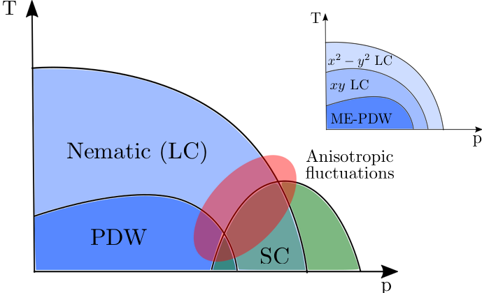
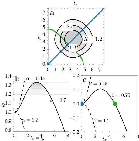
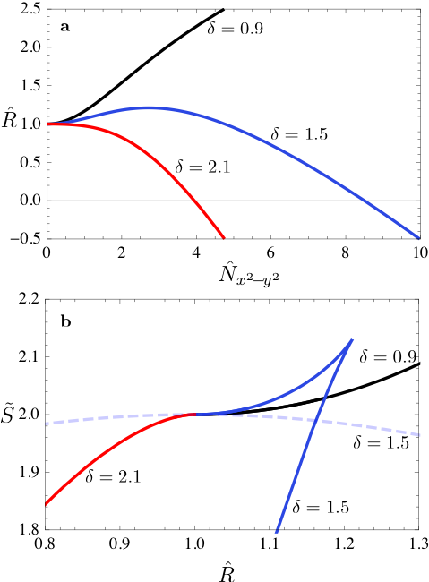
In this paper we explore the occurrence and competition between various PDW-vestigial phases, motivated both by an explicit model for stabilizing PDW order based on pair-hopping interactions[waardh2017effective; waardh2018suppression] (see also [wu2022pair]), and by recent experiments on strongly nematic phase fluctuations in a cuprate superconductor[wardh2019inprep]. First, we show how the relation between PDW and homogeneous superconductivity naturally generates an anisotropic superconducting state in a vestigial nematic PDW phase. In turn, this anisotropy can become strongly enhanced due to low phase-stiffness[emery1995importance; uemura1989universal], which in itself may also be related to a proximate PDW instability[waardh2017effective; waardh2018suppression]. Transport measurements in La2-xSrxCuO4 (LSCO) have shown evidence of an electronic nematic order[wu2017spontaneous]. These measurements indicate highly anisotropic superconducting fluctuations near the underdoped critical point, with only a small anisotropy of the normal electrons[wardh2019inprep]. This is consistent with the collective dynamics of the superconductor being highly susceptible to nematic order, along the lines presented in the present paper. A caricature of a phase diagram based on such a scenario, with interplay between superconductivity and vestigial PDW order, is presented in Figure 1.
In tetragonal symmetry, loop-current (LC) order is associated with a vector , transforming in the Eu representation. In the second part of the paper we will explore a scenario with an underlying ME-PDW state with LC order, which is invariant under reflection in the crystallographic diagonal (), with subleading (or B2g) nematic order . This phase is naturally preempted by a phase without the long-range PDW order but with vestigial LC and nematic order[agterberg2015emergent], which we refer to as an LC phase. We show that this preemptive transition can be split further into a low and and high-temperature phase. The low-temperature phase coincides with the LC phase, while the high-temperature phase breaks the tetragonal symmetry differently, by developing LC order which is invariant under reflection in the crystallographic axis , i.e. (or B1g) nematic order . We refer to this as an LC phase. Besides giving a richer phase diagram with both B1g and B2g symmetric orders, arising from the same underlying ME-PDW state, we find near the first-order transition between the and LC phase a state with approximate rotational symmetry in . This yields a very soft nematic order with is highly susceptible to external fields that may pin the nematic director away from the high symmetry directions.
I.1 Outline
This paper is composed of two main results parts and is outlined as follows. In Section II the considered model is discussed. This model is based on the phenomenology of an instability to a PDW state developed in[waardh2017effective; waardh2018suppression], but shares features with other discussed models for a PDW state[lee2014amperean; agterberg2015checkerboard; https://doi.org/10.48550/arxiv.2110.13138; setty2022exact; wu2022pair]. In the first results part, Section III, the model is decomposed into possible vestigial order parameters which is then used to develop an effective model of a uniform, but anisotropic, superconducting state, Eqn. 18. In Section III.2 we discuss how the proximity to a PDW instability, with concomitant vestigial nematic order, can give rise to a very large stiffness anisotropy of the superconductor.
II Model
A PDW state denotes a state where paired electrons have finite momenta . We consider the situation when a PDW state (with a spatially modulated superconducting order) is near degenerate with a homogeneous superconducting state. The partition function takes the form with
| (1) |
where . The action is given by the most general (2D) Ginzburg-Landau expression, with interaction , to fourth order in superconducting order, which respects gauge symmetry, translational symmetry, and the point-group symmetry . In order to describe an instability towards PDW order the superconducting ”dispersion” should develop minima at finite momenta. We consider a general dispersion to sixth order in in momenta
| (2) |
to ensure stability we take . This renormalized dispersion naturally occur in models with pair-hopping interactions[waardh2017effective; waardh2018suppression], but can also be considered a phenomenological model for coexisting zero- and finite-momentum superconductivity.
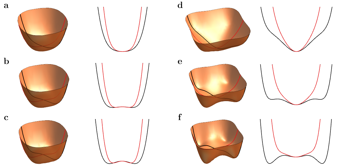
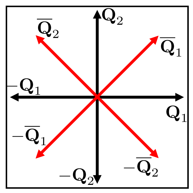
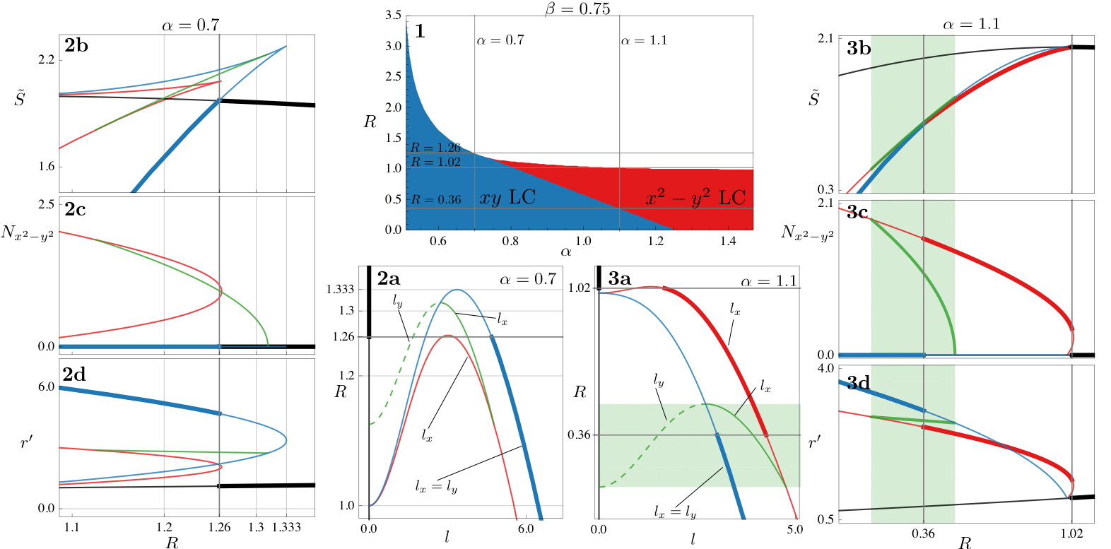
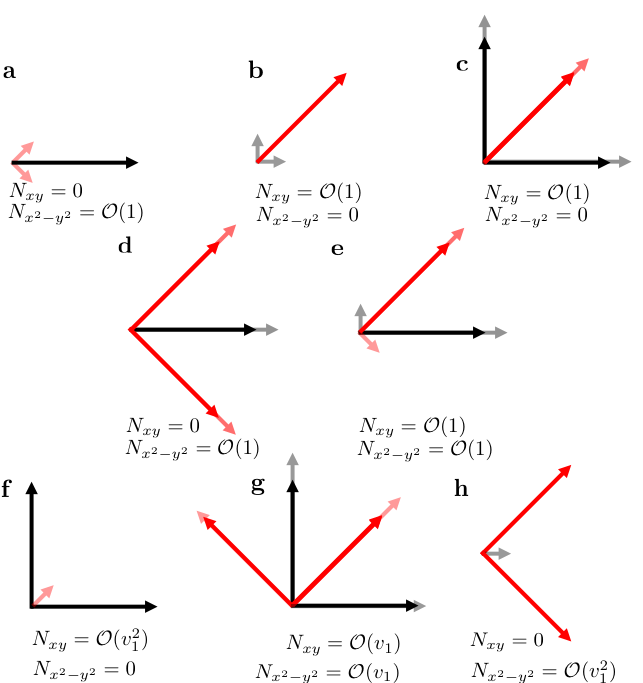
The instability to PDW order can occur in two different ways. The first, as shown in Figure 2a,b and c, is a continuous evolution of the pairing momenta from to finite , parametrized by going from positive to negative for . When the dispersion of the homogeneous superconductor becomes flat, constituting a Lifshitz-point, where the stiffness to fluctuations goes to zero. The second, occurring when and shown in Figure 2d,e and f, is a discontinuous jump in through the development of a distinct metastable state at finite momenta , which becomes stable when is decreased sufficiently. The dispersion (2) allows local minima both along the axes and the diagonals. In general eight finite momentum vectors are allowed given by , , and .
In order to analyze the fluctuations near the onset of these finite momentum orders we will go on re-expressing (1) by expanding in the various finite momentum superconducting order parameters. We will, however, leave the explicit form of the fourth order term in (1) unspecified and instead infer the expansion by considering all symmetry allowed terms. Before writing down the expression for the expanded action, we first discuss formally what terms are allowed.
II.1 Symmetry and order parameters
We consider the tetragonal point-group symmetry generated by , where is a four-fold rotation about the -axis, reflection in the plane and reflection in the plane. The different momenta of the PDW order leads to eight different complex order parameters, and one ordinary homogeneous superconducting field . The latter is assumed to be a single-component complex field, transforming in a one-dimensional representation of the point group, e.g. a wave order. The set of order parameters, , is divided into three sectors, A, B, and SC, . and contains the PDW fields, and do not transform into each other under , but their form is related by a twist. These are denoted by black and red in Figure 2. Besides the point-group symmetry, the action will be invariant under gauge symmetry, translational symmetry and time-reversal symmetry. Under these symmetries the order parameters transforms as , , and .
II.1.1 Composite order parameters
| Bilinears | Irrep. | ||
|---|---|---|---|
| A1g, | |||
| A1g, | |||
| B1g, | |||
| Eu, | |||
| A1g, | |||
| B2g, | |||
|
|
Eu, |
The action will be made up of all possible products of , that transform trivially under the full symmetry group . These will be second order, , and fourth order terms . (Terms including derivatives are discussed in Section II.1.2.) The possible vestigial phases will be described by a set of order parameters, , which are to second order in the primary fields , and transforming in non-trivial irreducible representations. We re-express the action in these composite order parameters, integrating out the PDW fields, . The new action will thus be made up of products of these composite order parameters, that transform trivially under the full symmetry group. The breaking of symmetries and emergence of vestigial phases is then understood in the language of a Landau phase transition where the order parameter develops a non-zero expectation value for , thus breaking the corresponding symmetry of the system.
We are especially interested in composite orders that only break the point-group symmetries, i.e. non-superconducting intra-unit cell orders. There are 9 bilinears that transforms trivially under , which we write as , where and . Again, and do not mix under and can be decomposed further into their irreducible representations: and , which are listed in Table 1.
The decomposition into bilinears implies the existence of two nematic order parameters, transforming as B1g and B2g, as well as two polar vector orders, transforming as Eu. The polar-vector order is odd under parity and has the symmetry of a toroidal moment, which shares symmetry with the so-called loop-current (LC) order, and we will refer to it as such. We will refer to an ME-PDW as a PDW with finite expectation value on LC order.
II.1.2 Derivative terms
Derivative terms arise by forming products between (transforming as Eu), and the bilinears . For , transforming as A1g, no linear derivative terms can arise to any order in . Mixing with PDW bilinears, transforming as , linear derivatives are allowed both to second and fourth order in fields. But, terms linear in derivatives implies an instability of the PDW momenta. Thus, expanding around stable local minima of (2), will to first non-vanishing order generate second-order terms in derivative and fields.
We do have the possibility of including derivative terms that are to fourth order in fields. However, usually, these terms are irrelevant compared to derivative terms arising to second order in fields. We will assume this is still true for the PDW fields, for which these terms will be neglected. However, near the Lifshitz point, where the dispersion for becomes flat, derivative terms acting on , occurring to fourth order in fields, will be important to include. To second order in derivatives and to fourth order in fields, we can form products between an A1g derivative term and the A1g bilinears, or the B1g(B2g) derivative term with the B1g(B2g) bilinears. The first term contributes to the isotropic stiffness and is of no particular interest (it can be included in the overall renormalization), the second type of term will, however, generate an anisotropic stiffness in the presence of (vestigial) nematic order from the PDW fields.
Terms linear in derivative do occur by coupling to the Eu bilinears. This coupling will shift the zero momentum in the presence of LC. But as long as the dispersion is well approximated with a parabola, this shift will not change the dispersion around the stable point, and the response will remain isotropic. Therefore we will neglect these terms even in the presence of LC order.
II.2 Expanded action
We find the expanded action (1) in terms of the irreducible representation discussed above as where contains the homogeneous superconducting field
| (3) |
the PDW fields, and their interaction. can be divided further, , one for each sector respectively, which will take the same form, but with independent parameters
| (4) |
where we absorbed a factor in all coefficients. As stated previously, the coefficients could be traced back to the exact form of the full Ginzburg-Landau model, 1, but we will consider them as independent parameters 111E.g. for a local interaction we find ..
has the same form as with and where . When in need of specifying both sectors we will append the subscript A or B to . The second-order term coefficient are assumed to be proportional to the temperature , changing sign at the mean-field transition temperature .
The interaction of the two sectors occurs in fourth-order terms and only involve the A1g and Eu representation of both sectors. Throughout the text, we will only explicitly assume a stable A sector, meaning that (2) only supports local minima of momenta along the axis, for which and drops out. However, we will reinsert the B sector when the result is directly generalizable. Discussion regarding the inclusion of both the A and B sectors are found in Appendix E. As mentioned above, we have left out terms consisting of bilinears that transform non-trivially under : , . These secondary order parameters refers to so-called 4e superconducting order[berg2009charge], which we neglect in subsequent analysis.
III Effective anisotropic superconductor
Now we will discuss the fate of the superconducting order in the presence of PDW vestigial order without any specific assumptions about the underlying instability or parameter regime. (Exploration of the ME-PDW vestigial phases is left for Section IV.) In the absence of long-range PDW order, , it is straightforward to integrate the PDW fields out, leaving an action only dependent on the vestigial order parameters and SC .
We begin by promoting the secondary order parameters to independent fields, which we do by decoupling the fourth-order terms in (4) using the Hubbard-Stratonovich transformation
| (5) |
Here is a vector of the bilinears listed in Table 1 and the corresponding vector of the auxiliary field to decouple that bilinear. The matrix is inferred from (4) and contains the coupling constants. We will assume only a stable A sector, yielding a diagonal . We denote the auxiliary fields with , dropping the A subindex, corresponding to the bilinear they decouple (see Table 1). Using this transformation, we express the partition function as
| (6) |
with the effective action given by
| (7) |
where and . We have left out the gauge field (absorbing it in the phase gradient), considering an extreme type-II superconductor, for which the electromagnetic field energy can be ignored. We will treat on a mean-field level and only keep the uniform component (i.e. etc.). The composite field will always have a non-zero and positive expectation value since it describes the fluctuations of the PDW state,
| (8) |
and is, therefore, not an order parameter. Similarly, developing a non-zero expectation value on any of the vestigial-orders parameters imply
| (9) |
respectively. Even in absence of PDW order we find non-equivalent uniform static susceptibilities once the vestigial order parameters are finite
| (10) |
here (see (24) for the full static susceptibilities). Without vestigial ordering, the transition temperature would be given by . Thus we see a splitting of the transition into the ordered PDW state and that the preemptive transition enhances the transition temperature.
III.1 Superconducting action
The effective action (7) can be written on the form
| (11) |
where is the volume, and we have moved to momentum representation.
The kernel is given by
| (12) |
Integrating over the PDW fields in (7) we arrive at the effective action for the vestigial and homogeneous superconducting fields alone
| (13) |
The new action takes the form
| (14) |
where
| (15) |
are functionals of the superconducting field. We expand the action in and around their mean-field values (see (23))
| (16) |
is the action at the mean-field solution, and the effective superconducting action. Above the superconducting transition temperature () we find
| (17) |
In real space the effective superconducting action takes the form
| (18) |
Here we have reintroduced both the A and B sectors and used the mean-field equations (23) to identify the order-parameters. (The mean-field equations for the two primary nematic orders remain unaltered even in the presence of both A and B sector, see Appendix E.)
The superconducting effective action (18) is expressed in terms of an anisotropic pair-mass (with ), induced by the nematic order parameters through the trace-less symmetric matrix . (Here we have only explicitly included the primary nematic fields, that are linear in the PDW fluctuations .) This anisotropic pair mass is equivalent to an anisotropic stiffness, that may be observed for example as an anisotropy of the in-plane penetration depth in the supercondcuting state, or through an anisotropy of the near normal state conductivity due to superconducting fluctuations [wardh2019inprep].
The coupling is the renormalized inverse static susceptibility. Since is single component, and its amplitude is rotationally symmetric, it cannot couple directly to the nematic order, as seen from the fact that only the symmetric PDW fluctuations contribute. As discussed in Section II.1.2, the expression (18) is expected to hold even in the presence of LC order, although the superconductor would acquire a small finite momentum.
III.2 Enhancement of anisotropic superconducting fluctuations near PDW instability
In (18) we have found an effective superconducting action, renormalized by the PDW fluctuations and the possible vestigial nematic order parameters and . Note that the superconductor is anisotropic in its dynamics, and at this level, the static order parameter is still isotropic. However, in the ordered SC state, the nematic order will affect the order parameter. In assuming d-wave superconductivity, there is a coupling (not considered here), which will induce a subleading s-wave component, effectively shifting the gap nodes. Nevertheless, as we argue below, for a superconductor with low phase stiffness, the effect of even a weak nematic field on the fluctuations may be dramatic, even though the effect on the static gap may be small.
As a digression, we note that this scenario of the effect of vestigial nematic order from superconducting fluctuations on the superconductor is similar in spirit but also different from electron-doped Bi2Se3. The latter has a multicomponent SC order parameter, which may itself form a vestigial nematic phase, which in turn would also affect the dynamics in the normal state[hecker2018vestigial]. In our case, instead, it is the finite momentum (PDW) superconducting components that give rise to the vestigial nematic order.
One way to probe the anisotropic stiffness of the superconductor is to study the contribution to the conductivity from superconducting fluctuations above , the paraconductivity. At , this contribution will diverge, reflecting the lifetime of Cooper pairs, and we expect to see a strong signature of the nematic order near . As derived in [wardh2019inprep], the Aslamazov-Larkin expression for the in-plane paraconductivity of a layered superconductor (inter-layer distance ) with anisotropic stiffness is given by
| (19) |
where refers to the principal axes of the conductivity, such that the last expression holds in the principal frame. Given a nematic distortion, in the form of (18), the pair-mass quotient is given by
| (20) |
where the angle of the axis (corresponding to the axis of highest conductivity) to the crystal -axis is given by
| (21) |
Thus, in the presence of both (i.e. ) and (i.e. ) the principal axes of conductivity will not be aligned with the symmetry axes of the crystal, and will rotate if the relative amplitude of the two fields change with temperature.
There is, in fact, evidence for highly anisotropic superconducting fluctuations in transport measurements done on thin films of underdoped LSCO [wu2017spontaneous; wardh2019inprep; bovzovic2023nematicity], consistent with a high pair-mass ratio . This ratio increases as the underdoped critical point is approached, while the quotient of normal masses remains near 1 [wardh2019inprep]. The crystals show very weak signs of lattice distortion, remaining effectively tetragonal, which is in line with the development of electronic nematicity coupling directly to the superconductor, and not through strain[wu2017spontaneous; bovzovic2023nematicity], consistent with the anisotropic superconductor described in (18). In addition, the principal axes of the paraconductivity (seen close to ) and the normal conductivity are in general not aligned with each other, or with the crystal axes, which is consistent with the presence of both and nematic order.
Nevertheless, the analysis leading up to (18) does not by itself explain why the superconducting stiffness-anisotropy would be enhanced compared to other observables that couple to nematicity, such as the normal electron conductivity, orthorhombic lattice distortions, and the superconducting gap (as discussed above). However, a natural explanation for this is evident in the expression for the pair-mass ratio (20); if the isotropic pair mass is sufficiently large (i.e. stiffness small), the quotient will become large even for a small nematic tensor . Without an explicit microscopic model of how the nematic order couples to normal and paired electrons this is only a qualitative statement, but that the phase stiffness is small in the underdoped cuprates is well-established[emery1995importance].
In fact, proximity to a PDW instability provides a unified conceptual framework in which both the low stiffness and the more recently observed nematic distortion thereof can be understood. As discussed in Section II, and more detailed in [waardh2018suppression], such an instability is expected to influence also the uniform component by deforming the spectrum of superconducting fluctuations giving a large effective pair mass. In other words, the availability of low energy finite momentum pair excitations suppresses the stiffness to real space deformations. Also, as we will further elucidate in the next section, the fluctuations of a (metastable) PDW state can generate vestigial nematic order that acts to deform the stiffness. Thus, approaching the finite momentum instability provides a mechanism for generating highly anisotropic superconducting fluctuations, both through creating a low phase-stiffness, yielding a high susceptibility towards an anisotropic distortion, as well as providing the distortion itself. This scenario is depicted in Figure 1, where the pseudogap is made up of vestigial phases set up by an underlying PDW state (possibly ME-PDW, as discussed in the following sections), with anisotropic superconducting fluctuations.
IV Intertwined nematic and loop-current orders in the vestigial ME-PDW phase
In this section we will investigate the various possible vestigial phases from an action of the form (4). Specifically we are interested in the nature of generation of the nematic order coupling to the dynamic response of the homogeneous superconductor through the action (18).
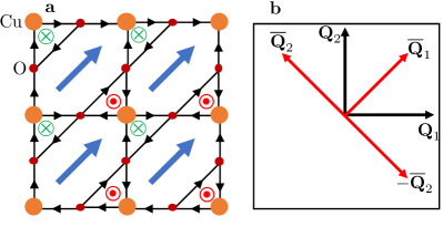
The ME-PDW state argued to be consistent with polarized ARPES measurements[kaminski2002spontaneous] has LC order corresponding to , which we will refer to as ME-PDW. In Figure 3a the PDW momenta for the ME-PDW state is shown alongside its circulating current analogue[simon2002detection]. As a speculative scenario for the cuprates, we will consider ME-PDW as a mean-field ground state for the pseudogap phase.
The overall stability of the action (4) requires . When no point-group symmetry is broken. For we have the possibility for nematic order without LC order, while is necessary for LC order. The mean-field solutions of in (4), and the corresponding stable vestigial phase, for are presented in Table 2. Here and subsequently, we use the notation
| (22) |
which parameterize the relative repulsion strength of fluctuation and primary nematic field. (The stability of the action (4) requires for and for .)
|
|
|
|
|
||||||||||||
|
|
|
LC | 1st | ||||||||||||
|
|
|
LC | 1st | ||||||||||||
|
|
|
LC |
|
||||||||||||
|
|
|
LC | 1st | ||||||||||||
|
|
|
(
|
|
||||||||||||
|
|
|
LC |
|
The mean-field state breaks both continuous gauge symmetry and the discrete point-group symmetry simultaneously. In the vestigial phase, the point-group symmetry breaking preempts the continuous symmetry breaking. Given that fluctuations act to restore the continuous symmetry, we expect that the vestigial phase breaks the same point-group symmetry as the mean-field solution. From this line of reasoning we expect to find a vestigial LC phase ( without long-range PDW order) above the transition to the ME-PDW. Surprisingly, for we find that the LC phase can become unstable to a LC phase () at higher temperature (see Figure 4). Thus, the mean-field ground state is preempted by a low-temperature vestigial phase, sharing the same symmetry, and a high-temperature vestigial phase, with a different symmetry (). This possibility can be understood as a result of a fluctuation induced transition between the mean-field ground and first excited state, which are both listed in Table 2. Near this transition we find a state with soft nematic order, which is discussed in Section IV.3 and V)
In the continuation of this section we derive the content of Table 2 and study the phase diagram for , presented in Figure 4. Some details are left for the Appendix A, B and C.
IV.1 Note on primary and subleading nematic orders
Again, for simplicity, we assume that only sector A is stable for the following development. However, it is important to note that the A and B sector supports different primary nematic fields, and respectively, while both supports the subleading nematic order and . A finite LC order implies subleading nematic order , transforming as B1g and B2g, respectively. The subleading nematic orders are to fourth order in PDW fields, while the primary nematic fields (listed in Table 1) are to second order in the PDW fields. Specifically, sector A only supports the primary nematic order , but not . Thus, an LC order, , implies subleading B2g nematic order, , but no primary, . In contrast, an LC order implies both secondary and primary B1g order, . (The reverse is true for the B sector.)
IV.2 Vestigial mean-field solutions
We will explore the possibility of vestigial-ordering by considering the mean-field solutions for , of the effective action (17), given by the solutions to the mean-field equations ,
| (23) |
where
| (24) |
are the static susceptibilities with , .
The most extreme example of a preemptive transition into a vestigial phase happens in 2D, where the integral for is infrared-divergent. This divergence leads to finite PDW susceptibilities (24), implying no long-range PDW order. This is just a restatement of the Mermin-Wagner theorem: Continuous symmetries will not form long-range order at finite temperature in 2D. The vestigial order parameters, however, being discrete Ising-like orders can break the point-group symmetries. Continuing with the 2D case, we find the mean-field equations of (17) as
| (25a) | ||||
| (25b) | ||||
| (25c) | ||||
| (25d) | ||||
where we introduced , , and as the momentum cut-off. Instead of using we have expressed the mean-field equations in terms of , where we assume . This is natural since describes Gaussian fluctuations of the PDW fields, which renormalizes the bare static susceptibility .
Care must be taken when considering solutions to (25). First, in the absence of long-range PDW order, only solutions fulfilling can be considered physical. Secondly, solutions to (25) are generally singular, meaning that solutions with finite order do not generally coincide with solutions without order in the limiting cases. Therefore we will have to consider all possible combinations of ordering independently. In addition to the trivial normal state without any ordering we find the following solutions
- (i)
-
(ii)
LC saddle-point solution: Unstable LC ordered state with both and nematic order, . Solutions are presented in Appendix A.
-
(iii)
LC state: LC ordered state with with nematic order, and . Solutions are presented in Appendix B.
Solutions with only nematic order and no LC order is of secondary interest and presented in Appendix D, for completeness.
In finding the vestigial mean-field solutions it is convenient to re-scale the order parameters to unit less quantities, , and equivalently for other variables. (See Appendix A and B for details.) However, for notational clearness we will suppress the tilde even when the parameters should be interpreted as unit less. The susceptibility gains an additional shift
| (26) |
Here is assumed to be tunable with temperature through its dependence on the bare susceptibility .
The mean-field solutions only guarantee local stability, and we must compare the absolute energy of the different phases in order to find the ground state. The energy is presented in Appendix C. The energy expression (42) was used to find the stable vestigial phases listed in Table2. For (), the () LC state is the stable state, regardless of (and for low enough ). In contrast, for , there is a transition between the and LC states for , as () is lowered, while the LC state is the only possible ordered state for . Thus, after including fluctuations, there is an induced transition between the would-be mean-field ground and first excited state (see Table 2), resulting in a high-temperature LC and low-temperature LC phase, separated by a first-order transition.
IV.3 Phase diagram and the and LC transition
As a representative case of , the phase diagram and the evolution of the order parameters is presented in Figure 4 for , and . (For the normal, and LC phase all coexist. It is possible to show that this holds in general for .)
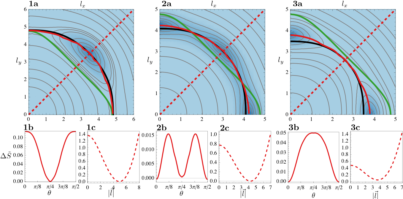
The saddle-point solution () only has support for a finite range of , as indicated by the green regions in Figure 4.3a-d, and forms closed paths in the -plane (see also Figure 7a in Appendix A). As is tuned from to , by lowering the temperature, twists from with to with .
To explore this transition further we consider the absolute energy in terms of 333Care must be taken when expressing the energy solely in terms of , see end of Appendix C. The energy is presented in Figure 5 for , just below () and above () the support for the saddle-point solution, as well as near the transition .
The and LC solutions lie on a semi-circular shaped valley in the energy landscape. Because of periodicity, the number of maxima equals the number of minima. Thus, in order for the and LC to be simultaneously stable, two intermediate maxima have to be introduced along the valley (in each quadrant). These are the solutions, and their energy can be seen as the height of the barrier between the two (meta)stable solutions. Nevertheless, these are saddle-point solutions in the full energy landscape. As is seen both from Figure 4.3b and Figure 5.2b, this barrier height is small compared to the energy scale in the radial direction. Thus, the solutions are easily excited along the valley-direction.
The relative smallness of the stiffness in the valley direction should be understood as a result of the valley direction being a compact dimension whose length is tunable to zero. Alternatively, it follows from expanding around a rotational invariant point . This effect is perhaps most easily seen from comparing Figure 5.1,3 with Figure 5.2. In the former, the dispersion is only about twice as soft in the valley direction, while in the latter, the inclusion of three additional stationary points forces the dispersion to become even flatter in the valley direction. In the limit , this feature is expected to become more pronounced. To confirm, we expand (39a) and (39b) for small , and find
| (27) |
describing two concentric circles. This implies that at all points around the valley will be arbitrarily close to a local maximum, thus the valley direction will be essentially flat. This expansion becomes exact for , and according to Table 2, there will be a second-order phase-transition for , where the and LC states are degenerate. Thus, the first-order transition gets tuned into second-order transition. As a corollary, we expect a small stiffness in the valley-direction whenever there is only a small region of support for the solutions.
V Soft nematic state
We have seen how the vicinity of the first-order transition between and LC gives rise to an arbitrarily flat energy landscape, associated with a rotation of the LC order. Thus, a small field would be able to pin the LC order in any direction, promoting a state with, in general, both B1g and B2g nematic order. For concreteness, we can consider a correction to the superconducting mass, like the one found in (18), due to the LC order
| (28) |
The principal direction of will in general not be aligned with the crystallographic axis, as well as being easily pinned in any direction. We will refer to this as a “soft” nematic state. (Note that does not constitute an nematic order parameter unless .)
There are some evidence for such a soft nematic state for the cuprates. A detachment of the nematic director from the lattice is seen in transport measurements on LSCO films[wu2017spontaneous]. A signature which is strongest near optimum doping. This state is also expected to be sensitive to quenched disorder, which might explain the decreasing nematic domain size in BSSCO[fujita2014simultaneous], approaching optimum doping. This would suggest that the underlying nematic state seen both in LSCO and BSSCO is of the same origin; an underlying ME-PDW preempted by a and/or LC state in turn setting up a soft nematic state, of the type described here; in LSCO the nematicity may be aligned by an external symmetry breaking field, while in BSCCO it is pinned to impurities. We include this scenario in the inset of Figure 1, where the vestigial nematic phase is divided in a high and low temperature phase with and nematic order respectively, with a soft nematic state at the boundary of the two phases.
V.1 Emergent overdamped Goldstone mode
The approximate rotational symmetry for the LC order near the first-order transition implies the existence of low-lying collective excitations. In the limit of an exact rotational symmetry this would corresponds to a Goldstone mode. To explore the the signatures of the soft nematic state near the transition we here consider the the spectral function of this “emergent” Goldstone mode.
The collective modes of the and LC states involves not only the LC order but couples all fields in the complete space; as change, and changes accordingly. Thus, in general, a collective mode is associated with variations in the combined space of . In (7), we neglected the time-dependence of the (bosonic) fields, corresponding to a high-temperature (classical) limit, where only the first bosonic Matsubara frequency is kept. Now we reintroduce the Matsubara frequencies to find the excitation spectra by analytic continuation to real frequencies.
The PDW part of the effective action (7) (for the A sector) can be written as
| (29) |
where we included an integral and fields in the Matsubara representation , with the bosonic Matsubara frequencies . We introduced the short-hand notation and , and . We find the kernel as
| (30) |
where , and . We assume that the PDW fields are coherently propagating, and not damped. (This would be the case if PDW arose from a strong-coupled BEC scenario[waardh2018suppression].) The effective action is found in terms of by integrating over the PDW fields. We proceed by expanding around the uniform mean-field solution , given by ,
| (31) |
Expanding the action to second order in
| (32) |
In the high-temperature limit, keeping only the first Matsubara term , is given by (14) (with reinserted). The correction can be written
| (33) |
Here is the propagator of fluctuations of , with . The self-energy term is given by
| (34) |
where
| (35) |
and where . The propagator is in general off-diagonal. However, when approaching the to LC transition from the LC state, with and , is block diagonal, . In this case the valley-direction lies solely along , with all other fields stationary.
The static, zero-frequency part of the propagator is associated with the stiffness to uniform deformation. Here can be related with the stiffness along the valley direction, which we set to zero and identify it with the transverse propagator for a nematic director along the -axis, . After analytic continuation of
| (36) |
we can obtain the retarded transverse propagator. In the high-temperature limit, after expanding in and (assuming , i.e. far from the PDW transition) we find
| (37) |
where , , , where is the angle of to the -axis.
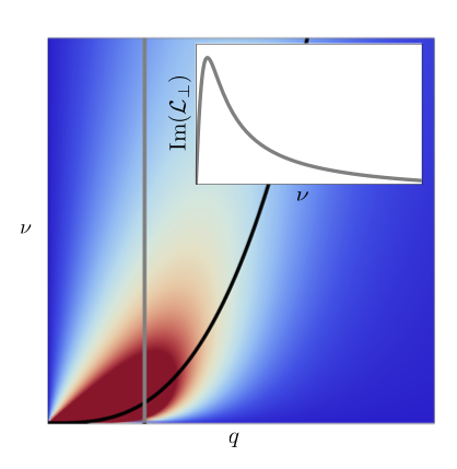
In Figure 6, the spectral density is shown, and we see an overdamped bosonic mode, with .
These results are reminiscent of the results for a nematic Fermi fluid[oganesyan2001quantum], where an overdamped Goldstone mode is found within the broken symmetry phase. (The reason has to do with the non-commuting property of the broken symmetry and translation[watanabe2014criterion].) In a fermionic system, an overdamped bosonic mode coupling to the fermions usually leads to the destruction of the Fermi liquid. This is of special interest in cuprates as a possible origin of the strange metal phase[keimer2015quantum; varma1989phenomenology].
A Goldstone mode associated with spatial rotation is not expected in a crystalline system since there is no rotational symmetry. However, as seen in this work, a competition between a vestigial and a LC phase leads to a very small gap and an emerging symmetry. It is intriguing to note that this phenomenology again points towards an emergent rotational symmetry near the overdoped critical point (possibly a soft nematic state), over which the strange metal phase is located. Indeed, at this level, these results are only speculative. First of all, in the model considered here, the bosonic mode does not couple directly to fermions, but to PDW fluctuations. The fate of the PDW fields, and the underlying fermions are left for future work.
VI Summary and Outlook
In this paper, we study vestigial orders of a PDW state with pair-momenta that are aligned with the high symmetry directions of a tetragonal crystal, focusing on phases that only break the point-group symmetry. Of particular interest is the influence of vestigial nematic order on a homogenous single component superconductor, giving rise to an anisotropic superfluid stiffness. We stress that if the nematicity arises from a PDW state, i.e., from finite momentum fluctuations of the superconducting field itself, the superconductor can become highly susceptible to this nematic distortion due to the natural proximity of a Lifshitz point with vanishing superfluid stiffness. Crucially, even a nominally weak nematic field, as observed through anisotropy of the normal electron response or the superconducting gap, may give a large relative renormalization of a small stiffness. We argue that this may explain why the observed anisotropy in transport measurements on LSCO [wu2017spontaneous] can be ascribed to highly anisotropic superconducting fluctuations coexisting with an essentially isotropic normal conductivity [wardh2019inprep]. Probing vortex dynamics, also expected to be sensitive to stiffness anisotropy, near , could be a fruitful pursuit to investigate this unusual manifestation of nematicity further.
In the later part of the paper we focus on vestigial orders of a magnetoelectric (ME) PDW, containing both nematic order and loop-current type order.We have shown that a preemptive transition into a vestigial phase of an ME-PDW with () nematic order can split into a high and low-temperature phase, that correspond to distinct and () phases. This feature is not specific to PDW, but is expected for any other field transforming in the (or ) representation. Near the transition between the high and low-temperature phases, the nematic order will be soft and easy to pin in either direction, yielding an approximate rotational symmetry, with possible relevance to observations of nematic order in LSCO and BSCCO. Also, as a start for further investigation, the emergence of an overdamped Goldstone mode due to this approximate rotational symmetry may have interesting implications for the single-particle properties of electrons coupling to this mode.
In conclusion, the results lend support and warrant further investigation into the proposal of pair-density wave order as the underlying source of the abundance of broken symmetries and exotic phenomenology seen in the cuprate superconductors.
Note: After the initial posting of this work an experimental study of overdoped Bi2Sr2CaCu2O8+x using scanning Josephson tunneling microscopy has presented evidence for a nematic state with short range PDW order, interpreted as a disorder-pinned realization of a state with vestigial nematic PDW order[chen2022identification].
VII Acknowledgements
We thank I. Božović for valuable discussions.
References
- Fradkin et al. [2015] E. Fradkin, S. A. Kivelson, and J. M. Tranquada, “Colloquium: Theory of intertwined orders in high temperature superconductors,” Reviews of Modern Physics 87, 457 (2015).
- Tranquada et al. [1995] J. M. Tranquada, B. J. Sternlieb, J. D. Axe, Y. Nakamura, and S. Uchida, “Evidence for stripe correlations of spins and holes in copper oxide superconductors,” Nature 375, 561 (1995).
- Ghiringhelli et al. [2012] G. Ghiringhelli, M. Le Tacon, M. Minola, S. Blanco-Canosa, C. Mazzoli, N. B. Brookes, G. M. De Luca, A. Frano, D. G. Hawthorn, F. He, et al., “Long-range incommensurate charge fluctuations in (Y,Nd)Ba2Cu3O6+x,” Science 337, 821–825 (2012).
- Chang et al. [2012] J. Chang, E. Blackburn, A. T. Holmes, N. B. Christensen, J. Larsen, J. Mesot, R. Liang, D. A. Bonn, W. N. Hardy, A. Watenphul, et al., “Direct observation of competition between superconductivity and charge density wave order in YBa2Cu3O6.67,” Nature Physics 8, 871 (2012).
- Le Tacon et al. [2014] M. Le Tacon, A. Bosak, S. M. Souliou, G. Dellea, T. Loew, R. Heid, K. P. Bohnen, G. Ghiringhelli, M. Krisch, and B. Keimer, “Inelastic X-ray scattering in YBa2Ca3O6.6 reveals giant phonon anomalies and elastic central peak due to charge-density-wave formation,” Nature Physics 10, 52 (2014).
- Keimer et al. [2015] B. Keimer, S. A. Kivelson, M. R. Norman, S. Uchida, and J. Zaanen, “From quantum matter to high-temperature superconductivity in copper oxides,” Nature 518, 179–186 (2015).
- Lawler et al. [2010] M. J. Lawler, K. Fujita, J. Lee, A. R. Schmidt, Y. Kohsaka, C. K. Kim, H. Eisaki, S. Uchida, J. C. Davis, J. P. Sethna, et al., “Intra-unit-cell electronic nematicity of the high-Tc copper-oxide pseudogap states,” Nature 466, 347 (2010).
- Fujita et al. [2014] K. Fujita, C. K. Kim, I. Lee, J. Lee, M. H. Hamidian, I. A. Firmo, S. Mukhopadhyay, H. Eisaki, S. Uchida, M.J. Lawler, et al., “Simultaneous transitions in cuprate momentum-space topology and electronic symmetry breaking,” Science 344, 612–616 (2014).
- Zheng et al. [2017] Y. Zheng, Y. Fei, K. Bu, W. Zhang, Y. Ding, X. Zhou, J. E. Hoffman, and Y. Yin, “The study of electronic nematicity in an overdoped (Bi,Pb)2Sr2CuO6+δ superconductor using scanning tunneling spectroscopy,” Scientific Reports 7, 8059 (2017).
- Wahlberg et al. [2021] Eric Wahlberg, Riccardo Arpaia, Götz Seibold, Matteo Rossi, Roberto Fumagalli, Edoardo Trabaldo, Nicholas B. Brookes, Lucio Braicovich, Sergio Caprara, Ulf Gran, Giacomo Ghiringhelli, Thilo Bauch, and Floriana Lombardi, “Restored strange metal phase through suppression of charge density waves in underdoped yba2cu3o7-δ,” Science 373, 1506–1510 (2021).
- Agterberg et al. [2020] D. F. Agterberg, J. S. Davis, S. D. Edkins, E. Fradkin, D. J. Van Harlingen, S. A. Kivelson, P. A. Lee, L. Radzihovsky, J. M. Tranquada, and Y. Wang, “The physics of pair-density waves: Cuprate superconductors and beyond,” Annual Review of Condensed Matter Physics 11, 231–270 (2020).
- Himeda et al. [2002] A. Himeda, T. Kato, and M. Ogata, “Stripe states with spatially oscillating d-wave superconductivity in the two-dimensional t-t’-j model,” Physical review letters 88, 117001 (2002).
- Fulde and Ferrell [1964] P. Fulde and R. A. Ferrell, “Superconductivity in a strong spin-exchange field,” Physical Review 135, A550 (1964).
- Larkin and Ovchinnikov [1965] A. I. Larkin and I. U. N. Ovchinnikov, “Inhomogeneous state of superconductors (Production of superconducting state in ferromagnet with fermi surfaces, examining green function),” Soviet Physics-JETP 20, 762–769 (1965).
- Berg et al. [2007] E. Berg, E. Fradkin, E-A. Kim, S. A. Kivelson, V. Oganesyan, J. M. Tranquada, and S. C. Zhang, “Dynamical layer decoupling in a stripe-ordered high-Tc superconductor,” Physical review letters 99, 127003 (2007).
- Berg et al. [2009a] E. Berg, E. Fradkin, and S. A. Kivelson, “Theory of the striped superconductor,” Physical Review B 79, 064515 (2009a).
- Moodenbaugh et al. [1988] A. R. Moodenbaugh, Y. Xu, M. Suenaga, T. J. Folkerts, and R. N. Shelton, “Superconducting properties of La2-x BaxCuO4,” Physical Review B 38, 4596 (1988).
- Li et al. [2007] Q. Li, M. Hücker, G. D. Gu, A. M. Tsvelik, and J. M. Tranquada, “Two-dimensional superconducting fluctuations in stripe-ordered La1.875Ba0.125CuO4,” Physical review letters 99, 067001 (2007).
- Li et al. [2010] L. Li, Y. Wang, S. Komiya, S. Ono, Y. Ando, G. D. Gu, and N. P. Ong, “Diamagnetism and cooper pairing above Tc in cuprates,” Physical Review B 81, 054510 (2010).
- Chakravarty et al. [2001] S. Chakravarty, R. B. Laughlin, D. K. Morr, and C. Nayak, “Hidden order in the cuprates,” Physical Review B 63, 094503 (2001).
- Lee [2014] P. A. Lee, “Amperean pairing and the pseudogap phase of cuprate superconductors,” Physical Review X 4, 031017 (2014).
- Baruch and Orgad [2008] S. Baruch and D. Orgad, “Spectral signatures of modulated d-wave superconducting phases,” Physical Review B 77, 174502 (2008).
- Zelli et al. [2011] M. Zelli, C. Kallin, and A. J. Berlinsky, “Mixed state of a -striped superconductor,” Physical Review B 84, 174525 (2011).
- Norman and Davis [2018] M. R. Norman and J. C. S. Davis, “Quantum oscillations in a biaxial pair density wave state,” Proceedings of the National Academy of Sciences 115, 5389–5391 (2018).
- Caplan and Orgad [2021] Yosef Caplan and Dror Orgad, “Quantum oscillations from a pair-density wave,” Phys. Rev. Research 3, 023199 (2021).
- Hamidian et al. [2016] M. H. Hamidian, S. D. Edkins, S. H. Joo, A. Kostin, H. Eisaki, S. Uchida, M. J. Lawler, E-A. Kim, A. P. Mackenzie, K. Fujita, et al., “Detection of a cooper-pair density wave in Bi2Sr2CaCu2O8+x,” Nature 532, 343–347 (2016).
- Edkins et al. [2019] S. D. Edkins, A. Kostin, K. Fujita, A. P. Mackenzie, H. Eisaki, S. Uchida, S. Sachdev, M. J. Lawler, E-A. Kim, J. C. Davis, et al., “Magnetic field–induced pair density wave state in the cuprate vortex halo,” Science 364, 976–980 (2019).
- Kaminski et al. [2002] A. Kaminski, S. Rosenkranz, H. M. Fretwell, J. C. Campuzano, Z. Li, H. Raffy, W. G. Cullen, H. You, C. G. Olson, C. M. Varma, et al., “Spontaneous breaking of time-reversal symmetry in the pseudogap state of a high-Tc superconductor,” Nature 416, 610 (2002).
- Fauqué et al. [2006] B. Fauqué, Y. Sidis, V. Hinkov, S. Pailhes, C. T. Lin, X. Chaud, and P. Bourges, “Magnetic order in the pseudogap phase of high-Tc superconductors,” Physical Review Letters 96, 197001 (2006).
- Li et al. [2008] Y. Li, V. Balédent, N. Barišić, Y. Cho, B. Fauqué, Y. Sidis, G. Yu, X. Zhao, P. Bourges, and M. Greven, “Unusual magnetic order in the pseudogap region of the superconductor HgBa2CuO4+δ,” Nature 455, 372 (2008).
- Li et al. [2011] Y. Li, V. Balédent, N. Barišić, Y. C. Cho, Y. Sidis, G. Yu, X. Zhao, P. Bourges, and M. Greven, “Magnetic order in the pseudogap phase of HgBa2CuO4+δ studied by spin-polarized neutron diffraction,” Physical Review B 84, 224508 (2011).
- Sidis and Bourges [2013] Y. Sidis and P. Bourges, “Evidence for intra-unit-cell magnetic order in the pseudo-gap state of high-Tc cuprates,” in Journal of Physics: Conference Series, Vol. 449 (IOP Publishing, 2013) p. 012012.
- Mangin-Thro et al. [2014] L. Mangin-Thro, Y. Sidis, P. Bourges, S. De Almeida-Didry, F. Giovannelli, and I. Laffez-Monot, “Characterization of the intra-unit-cell magnetic order in Bi2Sr2CaCu2o8+δ,” Physical Review B 89, 094523 (2014).
- Varma [2000] C. M. Varma, “Proposal for an experiment to test a theory of high-temperature superconductors,” Physical Review B 61, R3804 (2000).
- Simon and Varma [2002] M. E. Simon and C. M. Varma, “Detection and implications of a time-reversal breaking state in underdoped cuprates,” Physical review letters 89, 247003 (2002).
- Varma [2006] C. M. Varma, “Theory of the pseudogap state of the cuprates,” Physical Review B 73, 155113 (2006).
- Orenstein [2011] J. Orenstein, “Optical nonreciprocity in magnetic structures related to high-Tc superconductors,” Physical review letters 107, 067002 (2011).
- Yakovenko [2015] V. M. Yakovenko, “Tilted loop currents in cuprate superconductors,” Physica B: Condensed Matter 460, 159–164 (2015).
- Fernandes et al. [2012] R. M. Fernandes, A. V. Chubukov, J. Knolle, I. Eremin, and J. Schmalian, “Preemptive nematic order, pseudogap, and orbital order in the iron pnictides,” Physical Review B 85, 024534 (2012).
- Fernandes et al. [2014] R. M. Fernandes, A. V. Chubukov, and J. Schmalian, “What drives nematic order in iron-based superconductors?” Nature physics 10, 97 (2014).
- Fernandes et al. [2019] R. M. Fernandes, P. P. Orth, and J. Schmalian, “Intertwined vestigial order in quantum materials: nematicity and beyond,” Annual Review of Condensed Matter Physics 10, 133–154 (2019).
- Stanev and Tešanović [2010] Valentin Stanev and Zlatko Tešanović, “Three-band superconductivity and the order parameter that breaks time-reversal symmetry,” Phys. Rev. B 81, 134522 (2010).
- Bojesen et al. [2013] Troels Arnfred Bojesen, Egor Babaev, and Asle Sudbø, “Time reversal symmetry breakdown in normal and superconducting states in frustrated three-band systems,” Phys. Rev. B 88, 220511 (2013).
- Bojesen et al. [2014] Troels Arnfred Bojesen, Egor Babaev, and Asle Sudbø, “Phase transitions and anomalous normal state in superconductors with broken time-reversal symmetry,” Phys. Rev. B 89, 104509 (2014).
- Zeng et al. [2021] Meng Zeng, Lun-Hui Hu, Hong-Ye Hu, Yi-Zhuang You, and Congjun Wu, “Phase-fluctuation induced time-reversal symmetry breaking normal state,” (2021).
- Babaev et al. [2004] Egor Babaev, Asle Sudbø, and NW Ashcroft, “A superconductor to superfluid phase transition in liquid metallic hydrogen,” Nature 431, 666–668 (2004).
- Shibauchi et al. [2020] Takasada Shibauchi, Tetsuo Hanaguri, and Yuji Matsuda, “Exotic superconducting states in fese-based materials,” Journal of the Physical Society of Japan 89, 102002 (2020).
- Fernandes et al. [2022] R. M. Fernandes, A. I. Coldea, H. Ding, I. R. Fisher, P. J. Hirschfeld, and G. Kotliar, “Iron pnictides and chalcogenides: a new paradigm for superconductivity,” Nature 601, 35–44 (2022).
- Cho et al. [2020] C. Cho, J. Shen, J. Lyu, O. Atanov, Q. Chen, S. H. Lee, Y. S. Hor, D. J. Gawryluk, E. Pomjakushina, M. Bartkowiak, et al., “Z3-vestigial nematic order due to superconducting fluctuations in the doped topological insulators NbxBi2Se3 and CuxBi2Se3,” Nature communications 11, 1–8 (2020).
- Mukhopadhyay et al. [2019] Sourin Mukhopadhyay, Rahul Sharma, Chung Koo Kim, Stephen D Edkins, Mohammad H Hamidian, Hiroshi Eisaki, Shin-ichi Uchida, Eun-Ah Kim, Michael J Lawler, Andrew P Mackenzie, et al., “Evidence for a vestigial nematic state in the cuprate pseudogap phase,” Proceedings of the National Academy of Sciences 116, 13249–13254 (2019).
- Grinenko et al. [2021] Vadim Grinenko, Daniel Weston, Federico Caglieris, Christoph Wuttke, Christian Hess, Tino Gottschall, Ilaria Maccari, Denis Gorbunov, Sergei Zherlitsyn, Jochen Wosnitza, et al., “State with spontaneously broken time-reversal symmetry above the superconducting phase transition,” Nature Physics 17, 1254–1259 (2021).
- Nie et al. [2014] L. Nie, G. Tarjus, and S. A. Kivelson, “Quenched disorder and vestigial nematicity in the pseudogap regime of the cuprates,” Proceedings of the National Academy of Sciences 111, 7980–7985 (2014).
- Nie et al. [2017] L. Nie, A. V. Maharaj, E. Fradkin, and S. A. Kivelson, “Vestigial nematicity from spin and/or charge order in the cuprates,” Phys. Rev. B 96, 085142 (2017).
- Agterberg et al. [2015] D. F. Agterberg, D. S. Melchert, and M. K. Kashyap, “Emergent loop current order from pair density wave superconductivity,” Physical Review B 91, 054502 (2015).
- Wu et al. [2017] J. Wu, A. T. Bollinger, X. He, and I. Božović, “Spontaneous breaking of rotational symmetry in copper oxide superconductors,” Nature 547, 432 (2017).
- Wårdh et al. [2022] J. Wårdh, M. Granath, J. Wu, X. He, and I. Božović, “Colossal transverse magnetoresistance due to nematic superconducting phase fluctuations in a copper oxide,” arXiv preprint (2022), 10.48550/arXiv.2203.06769.
- Wårdh and Granath [2017] J. Wårdh and M. Granath, “Effective model for a supercurrent in a pair-density wave,” Physical Review B 96, 224503 (2017).
- Wårdh et al. [2018] J. Wårdh, B. M. Andersen, and M. Granath, “Suppression of superfluid stiffness near a lifshitz-point instability to finite-momentum superconductivity,” Physical Review B 98, 224501 (2018).
- Wu et al. [2022] Yi-Ming Wu, PA Nosov, Aavishkar A Patel, and S Raghu, “Pair density wave order from electron repulsion,” arXiv preprint arXiv:2209.09254 (2022).
- Emery and Kivelson [1995] V. J. Emery and S. A. Kivelson, “Importance of phase fluctuations in superconductors with small superfluid density,” Nature 374, 434 (1995).
- Uemura et al. [1989] Y. J. Uemura, G. M. Luke, B. J. Sternlieb, J. H. Brewer, J. F. Carolan, W. N. Hardy, R. Kadono, J. R. Kempton, R. F. Kiefl, S. R. Kreitzman, et al., “Universal correlations between and (carrier density over effective mass) in high-Tc cuprate superconductors,” Physical review letters 62, 2317 (1989).
- Agterberg and Garaud [2015] D. F. Agterberg and J. Garaud, “Checkerboard order in vortex cores from pair-density-wave superconductivity,” Physical Review B 91, 104512 (2015).
- Setty et al. [2021] Chandan Setty, Laura Fanfarillo, and P. J. Hirschfeld, “Microscopic mechanism for fluctuating pair density wave,” (2021), 10.48550/ARXIV.2110.13138.
- Setty et al. [2022] Chandan Setty, Jinchao Zhao, Laura Fanfarillo, Edwin W Huang, Peter J Hirschfeld, Philip W Phillips, and Kun Yang, “Exact solution for finite center-of-mass momentum cooper pairing,” arXiv preprint arXiv:2209.10568 (2022).
- Note [1] E.g. for a local interaction we find .
- Berg et al. [2009b] E. Berg, E. Fradkin, and S. A. Kivelson, “Charge-4e superconductivity from pair-density-wave order in certain high-temperature superconductors,” Nature Physics 5, 830–833 (2009b).
- Hecker and Schmalian [2018] M. Hecker and J. Schmalian, “Vestigial nematic order and superconductivity in the doped topological insulator CaxBi2Se3,” npj Quantum Materials 3, 26 (2018).
- Božović et al. [2023] Ivan Božović, Xi He, Anthony T Bollinger, and Roberta Caruso, “Is nematicity in cuprates real?” Condensed Matter 8, 7 (2023).
- Note [2] Only considering the A sector we do not find any primary () B2g nematic order, as discussed in IV.1.
- Note [3] Care must be taken when expressing the energy solely in terms of , see end of Appendix C.
- Oganesyan et al. [2001] V. Oganesyan, S. A. Kivelson, and E. Fradkin, “Quantum theory of a nematic fermi fluid,” Physical Review B 64, 195109 (2001).
- Watanabe and Vishwanath [2014] H. Watanabe and A. Vishwanath, “Criterion for stability of goldstone modes and fermi liquid behavior in a metal with broken symmetry,” Proceedings of the National Academy of Sciences 111, 16314–16318 (2014).
- Varma et al. [1989] C. M. Varma, P. B. Littlewood, S. Schmitt-Rink, E. Abrahams, and A. E. Ruckenstein, “Phenomenology of the normal state of Ca-O high-temperature superconductors,” Physical Review Letters 63, 1996 (1989).
- Chen et al. [2022] Weijiong Chen, Wangping Ren, Niall Kennedy, MH Hamidian, Shin-ichi Uchida, H Eisaki, Peter D Johnson, Shane M O’Mahony, and JC Séamus Davis, “Identification of a nematic pair density wave state in Bi2Sr2CaCu2o8+x,” Proceedings of the National Academy of Sciences 119, e2206481119 (2022).
Appendix A LC state and saddle-point solution,
Let us start by assuming that both and are nonzero. All equations (25) respects the symmetry , thus we can focus on . Non-trivial solutions of (25c)(25d) take the form
| (38) |
from which we see the need for to ensure . The existence of primary B1g nematic order, , is equivalent to as seen from (25b) which ensures if , while (25c),(25d) implies if , unless . Only considering the A sector we do not find any primary () B2g nematic order for the solution. However, if both the A and B sector were stable, the subleading () B2g nematic order would induce a finite primary B2g nematic order (supported by sector B) through the coupling set by in (4). In Appendix E we discuss the inclusion of both sectors, but for the present discussion this will be implicit.
Back to solving (25). Using (38) to simplify (25a) and (25b) we receive two new (reduced) mean-field equations
| (39a) | ||||
| (39b) | ||||
where we introduced the normalization , and . Note that equation (38) is not valid in the limit , since it implies , whereas (25c) and (25d) do not put any constraints on . Thus must be considered independently.
We find and by simultaneously solving (39a) and (39b), which we can interpret graphically as in Figure 7. Equation (39b) is always solved for , corresponding to (meta)stable solutions. Equation (39a) determines the evolution of , as is changed. For there is an onset of stable solutions at and , corresponding to a second-order phase-transition. For a locally stable solutions occur at a finite for some , implying a first-order phase-transition.
Equation (39b) also admits solutions with for , as can be seen from Figure 7. These solutions, only supported for a finite range in , will evolve along a curved path in the -plane, with a corresponding change in as changes. These solutions are unstable; however, as will be clarified, their existence indicates that a and a LC state are simultaneously stable. We will refer to this solution as the saddle-point solution since it constitutes a saddle-point in the energy landscape. Indeed, in the Section IV.3 we will see how admits a first-order transition between the and LC states, with the possibility of a superheated and supercooled phase.
Appendix B LC state,
Now we assume the stability of the LC solutions with only one finite LC order component, say . Equations (25d) puts no constraint on , while (25c) still implies . For physical solutions we must require as well as . In this case, we can directly solve for and using (25a) and (25b)
| (40a) | ||||
| (40b) | ||||
where denotes the product-logarithm. (For take and .) With , non-trivial solutions evolves as is lowered and (40a) starts admitting solutions. For and there is an onset of solutions at , corresponding to a second-order phase-transition. For solutions occur at a finite , corresponding to a first-order phase-transition. With similar arguments for , we find the transitions included in Table 2.
Appendix C Vestigial mean-field energy
The mean-field solutions only guarantee local stability, and we must compare the absolute energy of the different phases in order to find the ground state. Therefore, we need the normal-state solutions , as well, which are always admitted by (25b)(25c)(25d). Equation (25a) is readily solved by
| (41) |
requiring .
The energy (17) has an explicit dependence on the cutoff , which also renormalizes . In the limit the cutoff dependency can be absorbed in a constant energy term, given that the mean-field solution (25a) fulfilled
| (42) |
where . This energy was used to find the stable vestigial phases listed in Table 2.
It is important to note that the energy in 42 only holds if (25a) is fulfilled. In order to present the energy as a function solely on , as in Figure 5, we numerically solve (25a) and (25b) given an arbitrary by rewriting (25a),(25b) as first order differential equations. As boundary conditions (41) and were used at . The absolute energy in terms of was then found by inserting the solutions into (42).
Appendix D Additional solutions to the vestigial mean-field equations
One set of solutions that were not considered in the main development is that of only primary nematic order without loop-current(LC) order , the pure nematic phase. Equation (25c),(25d) always admits the solution, and puts no constraint on and . Non-trivial solutions to (25b) take the form
| (43) |
From which we find the expected requirement that we need , in order for . Assuming we can rewrite (43) as
| (44) |
which inserted in (25a) yields
| (45) |
where and . Equation (45) admits similar solutions as the LC case (39a) (see Figure 8), where we introduced . For there is one unstable branch for and none for . For there is an unstable branch for small and a stable one for bigger , which leads to a first-order transition. For there is one stable branch for and evolves continuously from zero, yielding a second-order transition.
So far has not entered the analysis and the solution is locally stable as long as , regardless of . For the pure nematic phase is the only locally stable solution. For , the and LC phases are in general stable as well and we have to compare the the absolute energy (42) of the different phases. Taking into account the general stability of (4) for we find that the pure nematic phase is stable for and the LC phase is stable for .
Appendix E Coupling between A and B sector
Bilinears of our model transforms in two distinct sectors, which we denote A and B. The stability of these two sectors, determined by the local minima of the dispersion (2), are independent, and we can consider situations where either one or both of the sectors are present.
The structures of both sectors are identical, and the above analysis holds equally for both sectors if we take into account that the states refer to the principal axes of
the A and B sector frame respectively, which are rotated 45∘ to each other. For concreteness, the LC and LC phase of the A sector map to the LC and LC phase of the B sector.
If both sectors are present they will couple through fourth order terms, tuned by in (4). We will study this situation by including a weak interaction between the two sectors. Including non-zero couplings in (4) means that the matrix in the Hubbard-Stratonovich transformation (5), will no longer be diagonal. Instead it will take the form
| (46) |
and the auxiliary field vector . Here is the B components along the () diagonals. After integrating out the PDW field the effective action is given by (neglecting the superconducting field, which can be analogously introduced as before)
| (47) |
The third term represents interaction between the A and B sectors, and the first two terms referring to the action of the A and B sectors respectively (17). Due to the inversion of the off-diagonal matrix, , the couplings become renormalized (indicated by the tilde in (47)) , , and . The two sectors do not couple directly through the primary nematic order-parameters . The bilinear term in the LC orders of the two sectors implies mutual induction: A finite LC order in one sector will induce LC order in the other sector. This is evident from the (new) mean-field equations
| (48a) | ||||
| (48b) | ||||
| (48c) | ||||
| (48d) | ||||
(analogously for the B sector). Assuming a weak mixing , we can expand in orders of . To first-order in we can solve the system by asserting , , where are solutions to the uncoupled case . To first order
| (49a) | |||
| (49b) | |||
| (49c) | |||
| (49d) | |||
and similar for the B sector. Here we used the static susceptibilities of the unperturbed state (24) and introduced . The correction to the vestigial mean-field solutions because of finite coupling between the sectors is illustrated in Figure 9, where black (red) arrows indicate the LC order in the A(B) sector. In Figure 9a the A sector is ordered in its LC state (), while the B sector is not ordered to zeroth order in . By turning on the coupling, an LC order in the B sector is induced . This state, being symmetric for reflections in the -axis, already has a finite expectation value for the primary nematic field, , in the unperturbed case (analogous case for the B sector is shown in Figure 9b). Similar cases is shown Figure 9c-e where no additional primary nematic order is induced, since it is present already for .
In contrast, for the case noted above, an LC phase in the A sector, which only have subleading nematic order, , the coupling will induce a primary nematic (stemming from the B sector). This is depicted in Figure 9f (and similarly in g,h).