Unified Visual Transformer Compression

Abstract

Vision transformers (ViTs) have gained popularity recently. Even without customized image operators such as convolutions, ViTs can yield competitive performance when properly trained on massive data. However, the computational overhead of ViTs remains prohibitive, due to stacking multi-head self-attention modules and else. Compared to the vast literature and prevailing success in compressing convolutional neural networks, the study of Vision Transformer compression has also just emerged, and existing works focused on one or two aspects of compression. This paper proposes a unified ViT compression framework that seamlessly assembles three effective techniques: pruning, layer skipping, and knowledge distillation. We formulate a budget-constrained, end-to-end optimization framework, targeting jointly learning model weights, layer-wise pruning ratios/masks, and skip configurations, under a distillation loss. The optimization problem is then solved using the primal-dual algorithm. Experiments are conducted with several ViT variants, e.g. DeiT and T2T-ViT backbones on the ImageNet dataset, and our approach consistently outperforms recent competitors. For example, DeiT-Tiny can be trimmed down to 50% of the original FLOPs almost without losing accuracy. Codes are available online: https://github.com/VITA-Group/UVC.

1 Introduction

Convolution neural networks (CNNs) (LeCun et al., 1989; Krizhevsky et al., 2012; He et al., 2016) have been the de facto architecture choice for computer vision tasks in the past decade. Their training and inference cost significant and ever-increasing computational resources.

Recently, drawn by the scaling success of attention-based models (Vaswani et al., 2017) in natural language processing (NLP) such as BERT (Devlin et al., 2018), various works seek to leverage the Transformer architecture to computer vision (Parmar et al., 2018; Child et al., 2019; Chen et al., 2020a). The Vision Transformer (ViT) architecture (Dosovitskiy et al., 2020), and its variants, have been demonstrated to achieve comparable or superior results on a series of image understanding tasks compared to the state of the art CNNs, especially when pretrained on datasets with sufficient model capacity (Han et al., 2021).

Despite the emerging power of ViTs, such architecture is shown to be even more resource-intensive than CNNs, making its deployment impractical under resource-limited scenarios. That is due to the absence of customized image operators such as convolution, the stack of self-attention modules that suffer from quadratic complexity with regard to the input size, among other factors. Owing to the substantial architecture differences between CNNs and ViTs, although there is a large wealth of successful CNN compression techniques (Liu et al., 2017; Li et al., 2016; He et al., 2017; 2019), it is not immediately clear whether they are as effective as for ViTs. One further open question is how to best integrate their power for ViT compression, as one often needs to jointly exploit multiple compression means for CNNs (Mishra & Marr, 2018; Yang et al., 2020b; Zhao et al., 2020b).

On the other hand, the NLP literature has widely explored the compression of BERT (Ganesh et al., 2020), ranging from unstructured pruning (Gordon et al., 2020; Guo et al., 2019), attention head pruning (Michel et al., 2019) and encoder unit pruning (Fan et al., 2019); to knowledge distillation (Sanh et al., 2019), layer factorization (Lan et al., 2019), quantization (Zhang et al., 2020; Bai et al., 2020) and dynamic width/depth inference (Hou et al., 2020). Lately, earlier works on compressing ViTs have also drawn ideas from those similar aspects: examples include weight/attention pruning (Zhu et al., 2021; Chen et al., 2021b; Pan et al., 2021a), input feature (token) selection (Tang et al., 2021; Pan et al., 2021a), and knowledge distillation (Touvron et al., 2020; Jia et al., 2021). Yet up to our best knowledge, there has been no systematic study that strives to either compare or compose (even naively cascade) multiple individual compression techniques for ViTs – not to mention any joint optimization like (Mishra & Marr, 2018; Yang et al., 2020b; Zhao et al., 2020b) did for CNNs. We conjecture that may potentially impede more performance gains from ViT compression.

This paper aims to establish the first all-in-one compression framework that organically integrates three different compression strategies: (structured) pruning, block skipping, and knowledge distillation. Rather than ad-hoc composition, we propose a unified vision transformer compression (UVC) framework, which seamlessly integrates the three effective compression techniques and jointly optimizes towards the task utility goal under the budget constraints. UVC is mathematically formulated as a constrained optimization problem and solved using the primal-dual algorithm from end to end. Our main contributions are outlined as follows:

• We present UVC that unleashes the potential of ViT compression, by jointly leveraging multiple ViT compression means for the first time. UVC only requires to specify a global resource budget, and can automatically optimize the composition of different techniques.

• We formulate and solve UVC as a unified constrained optimization problem. It simultaneously learns model weights, layer-wise pruning ratios/masks, and skip configurations, under a distillation loss and an overall budget constraint.

• Extensive experiments are conducted with popular variants of ViT, including several DeiT backbones and T2T-ViT on ImageNet, and our proposal consistently performs better than or comparably with existing methods.

  For example, UVC on DeiT-Tiny (with/without distillation tokens) yields around 50% FLOPs reduction, with little performance degradation (only 0.3%/0.9% loss compared to the uncompressed baseline).

2 Related Work

2.1 Vision transformer

Transformer (Vaswani et al., 2017) architecture stems from natural language processing (NLP) applications first, with the renowned technique utilizing Self-Attention to exploit information from sequential data. Though intuitively the transformer model seems inept to the special inductive bias of space correlation for images-oriented tasks, it has proved itself of capability on vision tasks just as good as CNNs (Dosovitskiy et al., 2020). The main point of Vision Transformer is that they encode the images by partitioning them into sequences of patches, projecting them into token embeddings, and feeding them to transformer encoders (Dosovitskiy et al., 2020). ViT outperforms convolutional nets if given sufficient training data on various image classification benchmarks.

Since then, ViT has been developed to various different variants first on data efficiency towards training, like DeiT (Touvron et al., 2020) and T2T-ViT (Yuan et al., 2021) are proposed to enhance ViT’s training data efficiency, by leveraging teacher-student and better-crafted architectures respectively. Then modifications are made to the general structure of ViT to tackle other popular downstream computer vision tasks, including object detection (Zheng et al., 2020; Carion et al., 2020; Dai et al., 2021; Zhu et al., 2020), semantic segmentation (Wang et al., 2021a; b), image enhancement (Chen et al., 2021a; Yang et al., 2020a), image generation (Jiang et al., 2021), video understanding (Bertasius et al., 2021), and 3D point cloud processing (Zhao et al., 2020a).

2.2 Model Compression

Pruning.

Pruning methods can be broadly categorized into: unstructured pruning (Dong et al., 2017; Lee et al., 2018; Xiao et al., 2019) by removing insignificant weight via certain criteria; and structured pruning (Luo et al., 2017; He et al., 2017; 2018; Yu et al., 2018; Lin et al., 2018; Guo et al., 2021; Yu et al., 2021; Chen et al., 2021b; Shen et al., 2021) by zero out parameters in a structured group manner. Unstructured pruning can be magnitude-based (Han et al., 2015a; b), hessian-based (LeCun et al., 1990; Dong et al., 2017), and so on. They result in irregular sparsity, causing sparse matrix operations that are hard to accelerate on hardware  (Buluc & Gilbert, 2008; Gale et al., 2019). This can be addressed with structured pruning where algorithms usually calculate an importance score for some group of parameters (e.g., convolutional channels, or matrix rows). Liu et al. (2017) uses the scaling factor of the batch normalization layer as the sensitivity metric. Li et al. (2016) proposes channel-wise summation over weights as the metric. Lin et al. (2020) proposes to use channel rank as sensitivity metric while  (He et al., 2019) uses the geometric median of the convolutional filters as pruning criteria. Particularly for transformer-based models, the basic structures that many consider pruning with include blocks, attention heads, and/or fully-connected matrix rows (Chen et al., 2020b; 2021b). For example,  (Michel et al., 2019) canvasses the behavior of multiple attention heads and proposes an iterative algorithm to prune redundant heads. (Fan et al., 2019) prunes entire layers to extract shallow models at inference time.

Knowledge Distillation.

Knowledge distillation (KD) is a special technique that does not explicitly compress the model from any dimension of the network. KD lets a student model leverage ··soft” labels coming from a teacher network (Hinton et al., 2015) to boost the performance of a student model. This can be regarded as a form of compression from the teacher model into a smaller student. The soft labels from the teacher are well known to be more informative than hard labels and leads to better student training (Yuan et al., 2020; Wei et al., 2020)

Skip Configuration.

Skip connection plays a crucial role in transformers  (Raghu et al., 2021), by tackling the vanishing gradient problem (Vaswani et al., 2017), or by preventing their outputs from degenerating exponentially quickly with respect to the network depth (Dong et al., 2021).

Meanwhile, transformer has an inborn advantage of a uniform block structure. A basic transformer block contains a Self-Attention module and a Multi-layer Perceptron module, and its output size matches the input size. That implies the possibility to manipulate the transformer depth by directly skipping certain layers or blocks.  (Xu et al., 2020) proposes to randomly replace the original modules with their designed compact substitutes to train the compact modules to mimic the behavior of the original modules.  (Zhang & He, 2020) designs a Switchable-Transformer Blocks to progressively drop layers from the architecture. To flexibly adjust the size and latency of transformers by selecting adaptive width and depth, DynaBERT (Hou et al., 2020) first trains a width-adaptive BERT and then allows for both adaptive width and depth. LayerDrop (Fan et al., 2019) randomly drops layers at training time; while at test time, it allows for sub-network selection to any desired depth.

3 Methodology

3.1 Preliminary

Vision Transformer (ViT) Architecture.

To unfold the unified algorithm in the following sections, here we first introduce the notations. There are totally $L$ transformer blocks. In each block $l$ of the ViT, there are two constituents, namely the Multi-head Self-Attention (MSA) module and the MLP module. Uniformly, each MSA for transformer block $l$ has $H$ attention heads originally.

In the Multi-head Self-Attention module, $W^{(l)}_{Q}$, $W^{(l)}_{K}$, $W^{(l)}_{V}$ are the weights of the three linear projection matrix in block $l$ that uses the block input $X^{l}$ to calculate attention matrices: $Q^{l}$, $K^{l}$, $V^{l}$. The weights of the projection module that follows self-attention calculation are denoted as $W^{(l,1)}$, represent the first linear projection module in block $l$. The MLP module consists of two linear projection modules $W^{(l,2)}$ and $W^{(l,3)}$.

Compression Targets

The main parameters that can be potentially compressed in a ViT block are $W^{(l)}_{Q}$, $W^{(l)}_{K}$, $W^{(l)}_{V}$ and $W^{(l,1)}$, $W^{(l,2)}$, $W^{(l,3)}$. Our goal is to prune the head number and head dimensions simultaneously inside each layer, associated with the layer level skipping, solved in a unified framework. Currently, we do not extend the scope to reduce other dimensions such as input patch number or token size. However, our framework can also pack these parts together easily.

For head number and head dimensions pruning, instead of going into details of QKV computation, we innovate to use $\{W^{(l,1)}\}_{1\leq l\leq L}$ to be the proxy pruning targets. Pruning on these linear layers is equivalent to the pruning of head number and head dimension. We also add $\{W^{(l,3)}\}_{1\leq l\leq L}$ as our pruning targets, since these linear layers do not have dimension alignment issues with other parts, they can be freely pruned, while the output of $\{W^{(l,2)}\}$ should match with the dimension of block input. We do not prune $W^{(l)}_{Q}$, $W^{(l)}_{K}$, $W^{(l)}_{V}$ inside each head, since $Q^{l}$, $K^{l}$, $V^{l}$ should be of the same shape for computing self-attention.

Besides, skip connection is recognized as another important component to enhance the performance of ViTs (Raghu et al., 2021). The dimension between $X^{l}$ and the output of the linear projection module should be aligned. For this sake, $W^{(l,2)}$ is excluded from our compression. Eventually, the weights to be compressed in our subsequent framework are $\{W^{(l,1)},W^{(l,3)}\}_{1\leq l\leq L}$.

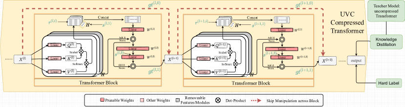
Figure 1: The overall framework of UVC, that integrates three compression strategies: (1) Pruning within a block: In a transformer block, we targeting on pruning Self-Attention head numbers ($s^{(l,1)}$), neuron numbers within a Self-Attention head ($r^{l,i}$) and the hidden size of MLP module ($s^{(l,3)}$) as well. (2) Skipping manipulation across blocks: When $\bm{gt}^{(l,0)}$ dominates, directly skip block $l$ and send $X^{l}$ into block $l+1$; Otherwise, pass $X^{l}$ into block $l$ without skip connection. (3) Knowledge distillation: The original uncompressed model is used to provide soft labels for knowledge distillation.

3.2 Resource-Constrained End-to-End ViT Compression

We target a principled constrained optimization framework jointly optimizing all weights and compression hyperparameters. We consider two strategies to compress ViT: (1) structural pruning of linear projection modules in a ViT block; and (2) adjusting the skipping patterns across different ViT blocks, including skipping/dropping an entire block. The second point, to our best knowledge, is the first time to be ever considered in ViT compression. The full framework is illustrated in Figure 1.

Alternatively, the two strategies could be considered as enforcing mixed-level group sparsity: the head dimension level, the head number level, and the block number level. The rationale is: when enforced with the same pruning ratios, models that are under finer-grained sparsity (i.e., pruning in smaller groups) are unfriendly to latency, while models that are under coarser-grained sparsity (i.e., pruning in larger groups) is unfriendly to accuracy. The mixed-level group sparsity can hence more flexibly trade-off between latency and accuracy.

The knowledge distillation is further incorporated into the objective to guide the end-to-end process. Below we walk through each component one-by-one, before presenting the unified optimization.

Pruning within a Block

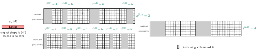
Figure 2: The two sparsity levels for pruning within a block: the head dimension level as controlled by $r^{(l,i)}$, and the head number level as controlled by $s^{(l,1)}$. When reaching the same pruning ratio, neuron-level sparsity will not remove any head, which is usually unfriendly to latency; while head level sparsity will only remove attention heads, which is usually unfriendly to accuracy.

To compress each linear projection module on width, we first denote $s^{(l,3)}$ as the number of columns to be pruned for weights $W^{(l,3)}$. Compression for weights $W^{(l,1)}$ is more complicated as it is decided by two degrees of freedom. As the input tensor to be multiplied with $W^{(l,1)}$ is the direct output of attention heads. Hence, within each layer $l$, we denote $s^{(l,1)}$ to be the attention head numbers that need to be pruned, and $r^{(l,i)}$ the number of output neurons to be pruned for each attention head $i$. Figure 2 illustrates the two sparsity levels: the head dimension level as controlled by $r^{(l,i)}$, and the head number level as controlled by $s^{(l,1)}$. They give more flexibility to transformer compression by selecting the optimal architecture in a multi-grained way. We emphasize again that those variables above are not manually picked, but rather optimized globally.

Skipping Manipulation across Blocks

The next component to jointly optimize is the skip connectivity pattern, across different ViT blocks. For vanilla ViTs, skip connection plays a crucial role in ensuring gradient flow and avoiding feature collapse (Dong et al., 2021). Raghu et al. (2021) suggests that skip connections in ViT are even more influential than in ResNets, having strong effects on performance and representation similarity. However, few existing studies have systematically studied how to strategically adjust skip connections provided a ViT architecture, in order to optimize the accuracy and efficiency trade-off.

In general, it is known that more skip connections help CNNs’ accuracy without increasing the parameter volume (Huang et al., 2017); and ViT seems to favor the same trend (Raghu et al., 2021). Moreover, adding a new skip connection over an existing block would allow us to “skip" it during inference, or “drop" it. This represents more aggressive “layer-wise" pruning, compared to the aforementioned element-wise or conventional structural pruning

While directly dropping blocks might look aggressive at the first glance, there are two unique enabling factors in ViTs that facilitate so. Firstly, unlike in CNNs, ViTs have uniform internal structures: by default, the input/output sizes of Self-Attention (SA) module, MLP module and thus the entire block, are all identical. That allows to painlessly drop any of those components and directly re-concatenating the others, without causing any feature dimension incompatibility. Secondly, Phang et al. (2021) observed that the top few blocks of fine-tuned transformers can be discarded without hurting performance, even with no further tuning. That is because deeper layer features tend to have high cross-layer similarities (while being dissimilar to early layer features), making additional blocks add little to the discriminative power. Zhou et al. (2021) also reported that in deep ViTs, the attention maps gradually become similar and even nearly identical after certain layers. Such cross-block “feature collapse" justifies our motivation to drop blocks.

In view of those, we introduce skip manipulation as a unique compression means to ViT for the first time.

Specifically, for each transformer block with the skip connection, we denote $gt^{(l,0)}$ and $gt^{(l,1)}$ as two binary gating variables (summing up to 1), to decide whether to skip this block or not.

The Constraints:

We next formulate weight sparsity constraints for the purpose of pruning. As discussed in Sec 3.1, the target of the proposed method is to prune the head number and head dimension simultaneously, which can actually be modeled as a two-level group sparsity problem when choosing $\{W^{(l,1)}\}_{1\leq l\leq L}$ as proxy compression targets. Specifically, the input dimension of $\{W^{(l,1)}\}_{1\leq l\leq L}$ is equivalent to the sum of the dimensions of all heads. Then we can put a two-level group sparsity regularization on $\{W^{(l,1)}\}_{1\leq l\leq L}$ input dimension to compress head number and head dimension at the same time, as shown in 1a and 1b. $r^{(l,i)}$ corresponding to the pruned size of $i_{th}$ head. $s^{(l,1)}$ means the pruned number of heads. For $\{W^{(l,3)}\}_{1\leq l\leq L}$, it is our compression target, we just perform standard one level group sparsity regularization on its input dimension, as shown in 1c.

$$\sum_{j}\mathbb{I}\left(\left\|\bm{W}_{g_{ij},.}^{(l,1)}\right\|_{2}^{2}=0\right)\geq r^{(l,i)},$$ (1a)

$$\sum_{i}\mathbb{I}\left(\left\|\bm{W}_{g_{i},.}^{(l,1)}\right\|_{2}^{2}=0\right)\geq s^{(l,1)},$$ (1b)

$$\sum_{i}\mathbb{I}\left(\left\|\bm{W}_{i,.}^{(l,3)}\right\|_{2}^{2}=0\right)\geq s^{(l,3)},\,$$ (1c)

$$\forall\,l=1,2,...,L,\forall\,i=1,2,...,H$$ (1d)

where $\bm{W}_{i,.}$ denotes the $i$-th column of $\bm{W}$; $\bm{W}_{g_{i},.}$ denotes the $i$-th grouped column matrix of $\bm{W}$, i.e. the $i$-th head; and $\bm{W}_{g_{ij},.}$ the $j$-th column of $\bm{W}_{g_{i},.}$, which is the $j$-th column of the $i$-th head. In other words, in Eqn. 1b, column matrices are grouped by attention heads. Hence among the original $H$ heads in total at block $l$, at least $s^{(l,1)}$ heads should be discarded. Similarly,  Eqn. 1c demands that at least $s^{(l,3)}$ input neurons should be pruned at this linear projection module. Furthermore,  Eqn. 1a requests that in the $i$-th attention head at block $l$, $r{(l,i)}$ of the output units should be set to zeros.

Our method is formulated as a resource constrained compression framework, given a target resource budget, it will compress the model until the budget is reached.

Given a backbone architecture, the FLOPs is the function of $\bm{s}$, $\bm{r}$ and $\bm{gt}$, denoted as $\mathcal{R}_{\textrm{Flops}}(\bm{s},\bm{r},\bm{gt})$. We have the constraint as:

$$\mathcal{R}_{\textrm{Flops}}(\bm{s},\bm{r},\bm{gt})\leq\mathcal{R}_{\textrm{budget}},\\$$ (2)

where $\bm{s}=\{s^{(l,1)},s^{(l,3)}\}_{1\leq l\leq L}$ and $\bm{r}=\{r^{(l,i)}\}_{1\leq l\leq L,1\leq i\leq H}$. $\mathcal{R}_{\textrm{budget}}$ is the resource budget. We present detailed flops computation equations in terms of $\bm{s}$, $\bm{r}$ and $\bm{gt}$ in Appendix.

Those inequalities can be further rewritten into equation forms to facilitate optimization. As an example, we follow (Tono et al., 2017) to reformulate  Eqn. 1b as:

$$\sum_{i}\mathbb{I}\left(\left\|\bm{W}_{.,g_{i}}\right\|_{2}^{2}=0\right)\geq s\Leftrightarrow\left\|\bm{W}_{\cdot,g}\right\|_{s,2}^{2}=0.$$ (3)

where $\left\|\bm{W}_{\cdot,g}\right\|_{s,2}^{2}$ denotes the Frobenius norm of the sub-matrix of $\bm{W}$ consisting of $s$ groups of $\bm{W}$ with smallest group norms.  Eqn. 1a and Eqn. 1c have same conversions.

The Objective:

The target objective could be written as ($\lambda$ is a coefficient):

$$\min_{\bm{W},\bm{gt}}\,\,\mathcal{L}(\bm{W},\bm{gt})=\ell(\bm{W},\bm{gt})+\lambda\ell_{distill}(\bm{W},\bm{W}_{t}),\\$$ (4)

where $\bm{W}_{t}$ denotes the weights from teacher model, i.e., the uncompressed transformer model, and $\ell_{distill}(*,*)$ is defined as the knowledge distillation loss. We choose the simper $\ell_{2}$ norm as its implementation, as its performance was found to be comparable to the more traditional K-L divergence (Kim et al., 2021).

The Final Unified Formulation:

Summarizing all above, we arrive at our unified optimization as a mini-max formulation, by leveraging the primal-dual method (Buchbinder & Naor, 2009):

$$\min_{{\bm{W}},\bm{s},\bm{r},\bm{gt}}\max_{\bm{p},\bm{y},z\geq 0}\mathcal{L}_{\textrm{pruning}}=\min_{{\bm{W}},\bm{s},\bm{r},\bm{gt}}\max_{\bm{p},\bm{y},z\geq 0}\mathcal{L}({\bm{W}},\bm{gt})+\underbrace{z\left(R_{\textrm{Flops}}(\bm{s},\bm{r},\bm{gt})-R_{\textrm{budget}}\right)}_{\textrm{resource loss}}+$$ (5)

$$\underbrace{\sum_{l=1}^{L}\bigg{(}y^{(l,1)}\left\|\bm{W}_{.,g}^{(l,1)}\right\|_{\lceil s^{(l,1)}\rceil,2}^{2}+y^{(l,3)}\left\|\bm{W}_{.,.}^{(l,3)}\right\|_{\lceil s^{(l,3)}\rceil,2}^{2}\bigg{)}+\sum_{l=1}^{L}\sum_{i=1}^{H}p^{(l,i)}\left\|\bm{W}_{.,g_{i}.}^{(l,1)}\right\|_{\lceil r^{(l,i)}\rceil,2}^{2}}_{\textrm{sparsity loss: }{\bm{S}}(\bm{y},\bm{s},\bm{p},\bm{r},\bm{gt},{\bm{W}})}$$

Eventually, we use the solution of the above mini-max problem, i.e. $\bm{s}$ and $\bm{r}$ to determine the compression ratio of each layer, and $\bm{gt}$ to determine the selection of skip configuration. Here, we select the pruned groups of the parameters by directly ranking columns by their norms, and remove those with the smallest magnitudes.

The general updating policy follows the idea of primal-dual algorithm. The full algorithm is outlined in  Algorithm 1 in Appendix. We introduce the solutions to each sub-problem in Appendix as well.

4 Experimental Results

Datasets and Benchmarks

We conduct experiments for image classification on ImageNet (Krizhevsky et al., 2012). We implement UVC on DeiT (Touvron et al., 2020), which has basically the identical architecture compared with ViT (Dosovitskiy et al., 2020) except for an extra distillation token; and a variant of ViT – T2T-ViT (Yuan et al., 2021), with a special token embedding layer that aggregates neighboring tokens into one token and a backbone with a deep-narrow structure. Experiment has been conducted on DeiT-Tiny/Small/Base and T2T-ViT-14 models. For DeiT-Tiny, we also try it without/with the distillation token. We measure all resource consumptions (including the UVC resource constraints) in terms of inference FLOPs.

Training Settings

The whole process of our method consists of two steps.

• Step 1: UVC training. We firstly conduct the primal-dual algorithm to the pretrained DeiT model to produce the compressed model under the given resource budget.

• Step 2: Post training. When we have the sparse model, we finetune it for another round of training to regain its accuracy loss during compression.

In the two steps mentioned above, we mainly follow the training settings of DeiT (Touvron et al., 2020) except for a relatively smaller learning rate which benefits finetuning of converged models.

For distillation, we select the pretrained uncompressed model to teach the pruned model.

Numerically, the learning rate for parameter $z$ is always changing during the primal-dual algorithm process. Thurs, we propose to use a dynamic learning rate for the parameter $z$ that controls the budget constraint. We use a four-step schedule of $\{1,5,9,13,17\}$ in practice.

Baseline methods

We adopt several latest compression methods which fall under two categories:

• Category 1: Input Patch Reduction, including $(i)$ PoWER (Goyal et al., 2020) : which accelerates language model BERT inference by eliminating word-vector in a progressive way. $(ii)$ HVT (Pan et al., 2021b): which reduce the token sequence dimension by using max-pooling hierarchically. $(iii)$ PatchSlimming (Tang et al., 2021): which identifies the effective patches in the last layer and then use them to guide the patch selection process of previous layers; and $(iv)$ IA-RED² (Pan et al., 2021a): which dynamically and hierarchical drops visual tokens at different levels using a learned policy network.

• Category 2: Model Weight Pruning, including $(v)$ SCOP (Tang et al., 2020): which is originally a channel pruning method used on CNN, we follow (Tang et al., 2021) and implement it on ViT. $(vi)$ Vision Transformer Pruning (VTP) (Zhu et al., 2021): which trains transformers with sparsity regularization to let important dimensions emerge. $(vii)$ SViTE (Chen et al., 2021b): which jointly optimizes model parameters and explores sparse connectivity throughout training, ending up with one final sparse network. SViTE belongs to the most competitive accuracy-efficiency trade-off achieved so far, for ViT pruning. We choose its structured variant to be fair with UVC.

4.1 Main Results

The main results are listed in  Tab. 1. Firstly, we notice that most existing methods cannot save beyond 50% FLOPs without sacrificing too much accuracy. In comparison, UVC can easily go with larger compression rates (up to $\geq$ 60% FLOPS saving) without compromising as much.

For example, when compressing DeiT-Tiny (with distillation token), UVC can trim the model down to a compelling $\geq$50% of the original FLOPs while losing only 0.3% accuracy (Tab. 3). Especially, compared with the latest SViTE (Chen et al., 2021b) that can only save up to around 30% FLOPs, we observe UVC to significantly outperform ig at DeiT-Tiny/Small, at less accuracy drops (0.9/0.4, versus 2.1/0.6) with much more aggressive FLOPs savings (50.7%/42.4%, versus 23.7%/31.63). For the larger DeiT-Base, while UVC can save 45% of its FLOPs, we fin that SViTE cannot be stably trained at such high sparsity. UVC also yield comparable accuracy with the other ViT model pruning approach, VTP (Zhu et al., 2021), with more than 10% FLOPs savings w.r.t. the original backbone.

Secondly, UVC obtains strong results compared with Patch Reduction based methods. UVC performs clearly better than IA-RED² (Pan et al., 2021a) at DeiT-Base, and outperforms HVT (Pan et al., 2021b) on both DeiT-Tiny/Small models, which are latest and strong competitors. Compared to Patch Slimming Tang et al. (2021), UVC at DeiT-Small reaches 79.44% top-1 accuracy, while the compression ratio measured by FLOPs is comparable. On other models, we observe UVC to generally save more FLOPs, yet also sacrificing more accuracies. Moreover, as we explained in Section 3.1, those input token reduction methods represent an orthogonal direction to the model weight sparsification way that UVC is pursuing. UVC can also be seamlessly extended to include token reduction into the joint optimization - a future work that we would pursue.

Thirdly, we test UVC on compressing T2T-ViT (Yuan et al., 2021). In the last row of  Tab. 1, UVC with 44% FLOPs achieves only a 2.6% accuracy drop. Meanwhile, UVC achieves a 1.9% accuracy drop with 51.5% of the original FLOPs. With 60.4% FLOPs, UVC only suffers from a 1.1% accuracy drop, already outperforming PoWER with 72.9% FLOPs.

Table 1: Comparison of the vision transformers compressed by UVC with different benchmarks on ImageNet. FLOPs remained denotes the remained ratio of FLOPs to the full-model FLOPs.

Model	Method	Top-1 Acc. (%)	FLOPs(G)	FLOPs remained(%)
DeiT-Tiny	Baseline	72.2	1.3	100
	SViTE	70.12 (-2.08)	0.99	76.31
	PatchSlimming	72.0 (-0.2)	0.7	53.8
	UVC	71.8 (-0.4)	0.69	53.1
	HVT	69.7 (-2.5)	0.64	49.23
	UVC	71.3 (-0.9)	0.64	49.23
	UVC	70.6 (-1.6)	0.51	39.12
DeiT-Small	Baseline	79.8	4.6	100
	SViTE	79.22 (-0.58)	3.14	68.36
	PoWER	78.3 (-1.5)	2.7	58.7
	UVC	79.44 (-0.36)	2.65	57.61
	SCOP	77.5 (-2.3)	2.6	56.4
	PatchSlimming	79.4 (-0.4)	2.6	56.5
	HVT	78.0 (-1.8)	2.40	52.2
	UVC	78.82 (-0.98)	2.32	50.41
DeiT-Base	Baseline	81.8	17.6	100
	IA-RED2	80.3 (-1.5)	11.8	67.04
	SViTE	82.22 (+0.42)	11.87	66.87
	VTP	80.7 (-1.1)	10.0	56.8
	PatchSlimming	81.5 (-0.3)	9.8	55.7
	UVC	80.57 (-1.23)	8.0	45.50
T2T-ViT-14	Baseline	81.5	4.8	100
	PoWER	79.9 (-1.6)	3.5	72.9
	UVC	80.4 (-1.1)	2.90	60.4
	UVC	79.6 (-1.9)	2.47	51.5
	UVC	78.9 (-2.6)	2.11	44.0

Table 2: Ablation study on the modules implemented in UVC. The first part present single technique ablation. The second part presents the result to sequentially apply Skip configuration and Pruning.

Method	DeiT-Tiny
	Acc. (%)	FLOPs remained(%)
Uncompressed baseline	72.2	100
Only skip manipulation	68.72	51.85
Only pruning within a block	70.52	50.69
Without Knowledge Distillation	69.34	51.23
Skip$\to$Prune 71.49%$\to$49.39%	66.84	49.39
Prune$\to$Skip 69.96%$\to$54.88%	69.68	54.88
Prune$\to$Skip 63.25%$\to$50.73%	70.02	50.73
UVC	71.3	49.23

4.2 Ablation study

As UVC highlights the integration of three different compression techniques into one joint optimization framework, it would be natural to question whether each moving part is necessary for the pipeline, and how they each contribute to the final result. We conduct this ablation study, and the results are presented in Tab. 2.

Skip Manipulation only.

We first present the result when we only conduct skip manipulation and knowledge distillation in our framework, but not pruning within a block. All other protocols remain unchanged. This two-in-a-way method is actually reduced into LayerDropping (Lin et al., 2018). We have the following findings: Firstly, implementing only skip connection manipulation will incur high instability. During optimization, the objective value fluctuates heavily due to the large architecture changes (adding or removing one whole block) and barely converges to a stable solution. Secondly, only applying skip manipulation will be damaging the accuracy remarkably, e.g., by nearly 4% drop on DeiT-Tiny. That is expected, as only manipulating the model architecture with such a coarse granularity (keeping or skipping a whole transformer block) is very inflexible and prone to collapse.

Pruning within a Block only.

We then conduct experiments without using the gating control for skip connections. That leads to only integrating neuron-level and attention-head-level pruning, with knowledge distillation. It turns out to deliver much better accuracy than only skip manipulation, presumably owing to its finer-grained operation. However, it still has a margin behind our joint UVC method, as the latter also benefits from removing block-level redundancy a priori, which is recently observed to widely exist in fine-tuned transformers Phang et al. (2021). Overall, the ablation results endorse the effectiveness of jointly optimizing those components altogether.

Applying Individual Compression Methods Sequentially

Our method is a joint optimization process for skip configuration manipulation and pruning, but is this joint optimization necessary?

To address this curiosity, we mark Prune$\to$Skip as the process of pruning first, manipulating skip configuration follows, while Skip$\to$Prune vice versa. Note that Skip$\to$Prune 71.49%$\to$49.39% denotes the pipeline that use skip configuration first to enforce the model FLOPs to be 71.49% of the original FLOPs, then apply pruning to further compress the model to 49.39%. Without loss of generality, we approximate both the pruning procedure and skipping procedure to compress 70% of the previous model, which will approximately result in a model with 50% of the original FLOPs. Based on this, we implement:$(i)$ Skip$\to$Prune 71.49%$\to$49.39% It first compresses the model to 71% by skipping then applies pruning on the original model and results in the worse performance at 66.84%. $(ii)$Prune$\to$Skip 69.96%$\to$54.88% It applies pruning to 70% FLOPs then skipping follows. We observe that applying pruning first can stabilize the choice of skip configuration and result in a top-1 accuracy of 69.68%. Both results endorse the superior trade-off found by UVC.

Furthermore, we design a better setting (Prune$\to$Skip 63.25%$\to$50.73%) to simulate the compression ratio found by UVC. Details can be found in Appendix. The obtained result is much better than previous ones, but still at a 1% performance gap from the result provided by UVC. We assign the extra credit to jointly optimizing the architecture and model weights.

5 Conclusion

In this paper, we propose UVC, a unified ViT compression framework that seamlessly assembles pruning, layer skipping, and knowledge distillation as one. A budget-constrained optimization framework is formulated for joint learning. Experiments demonstrate that UVC can aggressively trim down the prohibit computational costs in an end-to-end way. Our future work will extend UVC to incorporating weight quantization as part of the end-to-end optimization as well.

Appendix A Appendix

A.1 Updating policy

Updating Weights ${\bm{W}}$

Different from other pruning methods in CNN that use fixed pre-trained weights to select the pruned channels/groups with certain pre-defined metrics (Lin et al., 2020; He et al., 2019), here our subproblem could be considered as following dynamic pruning criteria that will be updated along. Specifically, we solve the following subproblem:

$$\textrm{Prox}_{\eta_{1}{\bm{S}}\left(\bm{y},\bm{s},\bm{p},\bm{r},{\bm{W}}\right)}(\bar{{\bm{W}}})={\textrm{arg}\min}_{{\bm{W}}}\,\,\frac{1}{2}\left\|{\bm{W}}-\bar{{\bm{W}}}\right\|^{2}+\eta_{1}{\bm{S}}\left(\bm{y},\bm{s},\bm{p},\bm{r},{\bm{W}}\right),$$ (6)

where $\bar{{\bm{W}}}={\bm{W}}^{t}-\eta_{1}\hat{{\nabla}}_{{\bm{W}}}\ell\left({\bm{W}}^{t}\right)$. The solution admits a bi-level projection (Yang et al., 2016):

$$\bm{W}^{(l,1)*}_{.,g_{ij}}=\begin{cases}\bar{\bm{W}}_{.,g_{ij}}^{(l,1)},\quad&\textrm{if $\left\|\bar{\bm{W}}_{.,g_{ij}}^{(l,1)}\right\|_{2}^{2}\geq\left\|\bm{W}_{.,g_{i\textrm{least-}\lceil r^{(l,i)}\rceil}}^{(l,1)}\right\|_{2}^{2}$},\\ \frac{1}{1+2\eta_{1}p^{(l,i)}}\bar{\bm{W}}_{i},&\textrm{otherwise},\end{cases}$$

$$\bm{W}^{(l,1)*}_{.,g_{i}}=\begin{cases}\bar{\bm{W}}_{.,g_{i}}^{(l,1)},\quad&\textrm{if $\left\|\bar{\bm{W}}_{.,g_{i}}^{(l,1)}\right\|_{2}^{2}\geq\left\|\bm{W}_{.,g_{\textrm{least-}\lceil s^{(l,1)}\rceil}}^{(l,1)}\right\|_{2}^{2}$},\\ \frac{1}{1+2\eta_{1}y^{(l,1)}}\bar{\bm{W}}_{.,g_{i}},&\textrm{otherwise},\end{cases}$$

$$\bm{W}^{(l,3)*}_{.,i}=\begin{cases}\bar{\bm{W}}_{.,i}^{(l,3)},\quad&\textrm{if $\left\|\bar{\bm{W}}_{.,i}^{(l,3)}\right\|_{2}^{2}\geq\left\|\bm{W}_{.,\textrm{least-}\lceil s^{(l,3)}\rceil}^{(l,3)}\right\|_{2}^{2}$},\\ \frac{1}{1+2\eta_{1}y^{(l,3)}}\bar{\bm{W}}_{.,i},&\textrm{otherwise},\end{cases}$$

where least-$j$ denotes the index of the (group) columns of $\bm{W}$ that have $j$-th least (group) norm.

Updating $\bm{gt}$

$\bm{gt}^{l}=(\bm{gt}^{(l,0)},\bm{gt}^{(l,1)})$ are used to generate a binomial categorical distribution to decide whether pass through block $l$ or directly skip it. As the two variables are discrete, we apply the renowned Gumbel-Softmax (GSM) trick (Jang et al., 2016) to obtain differentiable and polarized sampling. For $\bm{gt}^{l}=(\bm{gt}^{(l,0)},\bm{gt}^{(l,1)})$, given i.i.d Gumbel noise $g$ drawn from $Gumbel(0,1)$ distribution, a soft categorical sample can be drawn by

$$G^{l}=GSM(\bm{gt}^{l})=Softmax((log(\bm{gt}^{l})+g)/\tau)\in\mathbb{R}^{2},$$ (7)

where $G^{(l,1)}$ refers to the continuous possibility to preserve current block $l$ while $G^{(l,0)}$ to drop it.

Directly applying the chain rule on $\mathcal{L}(\bm{W},\bm{gt})$ w.r.t $\bm{gt}$ can now calculate $\tilde{\nabla}_{\bm{gt}}\mathcal{L}({\bm{W}}^{t},\bm{gt}^{t})$.

Also, $\bm{gt}$ participates in the calculation of FLOPs, by deciding whether to pass certain blocks. Since passing or skipping a block is a dynamic choice during training, we estimate the FLOPs of the $l$-th block $\mathcal{R}_{\textrm{Flops}}(\bm{s},\bm{r},\bm{gt})$ with skip gating by using its expectation. To be specific,

$$\mathcal{R}_{\textrm{Flops}_{l}}(\bm{s}_{l},\bm{r}_{l},\bm{gt}_{l}) =\mathbb{E}[\mathcal{R}_{\textrm{Flops}_{l}}(\bm{s}_{l},\bm{r}_{l},\bm{gt}_{l})|\bm{s}_{l},\bm{r}_{l}]$$ (8a)

$$=G^{(l,0)}\mathcal{R}_{\textrm{Flops}_{l}}(Identity)+G^{(l,1)}\mathcal{R}_{\textrm{Flops}_{l}}(\bm{s}_{l},\bm{r}_{l})$$ (8b)

$$=G^{(l,1)}\mathcal{R}_{\textrm{Flops}_{l}}(\bm{s}_{l},\bm{r}_{l})$$ (8c)

Hence, updating policy for $\bm{gt}$ is formulated as:

$$\bm{gt}^{t+1} =\bm{gt}^{t}-\eta_{4}\ \left(\tilde{\nabla}_{\bm{gt}}\mathcal{L}\left({\bm{W}},\bm{gt}^{t}\right)+\tilde{\nabla}_{\bm{gt}}z\left(R_{\textrm{Flops}}\left(\bm{s},\bm{r},\bm{gt}^{t}\right)-R_{\text{budget}}\right)\right)$$ (9)

$$=\bm{gt}^{t}-\eta_{4}\ \left(\tilde{\nabla}_{\bm{gt}}\mathcal{L}\left({\bm{W}},\bm{gt}^{t}\right)+\tilde{\nabla}_{\bm{gt}}zR_{\textrm{Flops}}(\bm{s},\bm{r})GSM(\bm{gt}^{t})\right)$$ (10)

Updating $\bm{s}$ and $\bm{r}$

Similar to the updating policy of $\bm{gt}$, one gradient term w.r.t. $\bm{s}$ and $\bm{r}$ are $\tilde{\nabla}_{\bm{s}}z\left(R_{\textrm{Flops}}\left(\bm{s},\bm{r},\bm{gt}\right)-R_{\text{budget}}\right)$, $\tilde{\nabla}_{\bm{r}}z\left(R_{\textrm{Flops}}\left(\bm{s},\bm{r},\bm{gt}\right)-R_{\text{budget}}\right)$ respectively.

The other gradient term is calculated on the unified formulation Eqn. 5. Refer to that, $\bm{s}$ and $\bm{r}$ are floating-point numbers during the optimization process. In practise, ceiling functions are operated on them to determine the integer number that should be pruned for each layer. However, the ceiling function $\lceil.\rceil$ is non-differentiable. To solve this problem, we implement Straight-through estimator(STE) (Bengio et al., 2013) to provide a proxy of the gradient when performing the backward pass. We set $\frac{\tilde{\partial}\lceil s\rceil}{\tilde{\partial}s}=1.$

As for $\left\|\bm{W}_{.,g}\right\|_{s,2}^{2}$ term in the sparsity loss, we use $\left\|\bm{W}_{.,g}\right\|_{s+1,2}^{2}-\left\|\bm{W}_{.,g}\right\|_{s,2}^{2}$ as the proxy of partial derivative of $\left\|\bm{W}_{.,g}\right\|_{s,2}^{2}$ with respect to $s$:

$$\frac{\tilde{\partial}\left\|\bm{W}_{.,g}\right\|_{s,2}^{2}}{\tilde{\partial}s}=\left\|{\bm{W}_{.,g_{\textrm{least-min}\{\textrm{Dim}(\bm{W}),s+1\}}}}\right\|_{2}^{2},$$ (11)

where Dim$(\bm{W})$ is the number of column groups of $\bm{W}$. The other two terms in the sparsity loss can be processed similarly.

A.2 Main Algorithm

The general updating policy follows the idea of primal-dual algorithm. The full algorithm is outlined in  Algorithm 1.

1

Input: Resource budget $R_{\text{budget}}$, learning rates $\eta_{1},\eta_{2},\eta_{3},\eta_{4},\eta_{5},\eta_{6}$, number of total iterations $\tau$.

Result: Transformer pruned weights ${\bm{W}}^{*}$.

Initialize $t=1,{\bm{W}}^{1}$ ;

  // random or a pre-trained dense model

2 for $t\leftarrow 1$ to $\tau$ do

       ${\bm{W}}^{t+1}=\textrm{Prox}_{\eta_{1}{\bm{S}}\left(\bm{y}^{t},\bm{s}^{t},\bm{p}^{t},\bm{r}^{t},{\bm{W}}^{t}\right)}\left({\bm{W}}^{t}-\eta_{1}\hat{{\nabla}}_{{\bm{W}}}\mathcal{L}\left({\bm{W}}^{t},\bm{gt}\right)\right)$ ;

        // Proximal-SGD

       $\bm{s}^{t+1}=\bm{s}^{t}-\eta_{2}\ \left(\tilde{\nabla}_{\bm{s}}{\bm{S}}\left(\bm{y}^{t},\bm{s}^{t},\bm{p}^{t},\bm{r}^{t},\bm{gt}^{t},{\bm{W}}^{t+1}\right)+\tilde{\nabla}_{\bm{s}}z^{t}\left(R_{\textrm{Flops}}\left(\bm{s}^{t},\bm{r}^{t},\bm{gt}^{t}\right)-R_{\text{budget}}\right)\right)$ ;

        // Gradient (STE) Descent

       $\bm{r}^{t+1}=\bm{r}^{t}-\eta_{3}\ \left(\tilde{\nabla}_{\bm{r}}{\bm{S}}\left(\bm{y}^{t},\bm{s}^{t+1},\bm{p}^{t},\bm{r}^{t},\bm{gt}^{t},{\bm{W}}^{t+1}\right)+\tilde{\nabla}_{\bm{r}}z^{t}\left(R_{\textrm{Flops}}\left(\bm{s}^{t+1},\bm{r}^{t},\bm{gt}^{t}\right)-R_{\text{budget}}\right)\right)$ ;

        // Gradient (STE) Descent

       $\bm{gt}^{t+1}=\bm{gt}^{t}-\eta_{4}\ \left(\tilde{\nabla}_{\bm{gt}}\mathcal{L}\left({\bm{W}}^{t+1},\bm{gt}^{t}\right)+\tilde{\nabla}_{\bm{gt}}z^{t}\left(R_{\textrm{Flops}}\left(\bm{s}^{t+1},\bm{r}^{t+1},\bm{gt}^{t}\right)-R_{\text{budget}}\right)\right)$ ;

        // Gradient Descent

        $z^{t+1}=z^{t}+\eta_{7}\left(R_{\textrm{Flops}}\left(\bm{s}^{t+1},\bm{r}^{t+1},\bm{gt}^{t+1}\right)-R_{\text{budget}}\right)$ ;

        // Gradient Ascent

       ${y^{(l,1)}}^{t+1}={y^{(l,1)}}^{t}+\eta_{5}\left(\left\|{\bm{W}_{.,g}^{(l,1)}}^{t+1}\right\|_{\left\lceil{s^{(l,1)}}^{t+1}\right\rceil,2}^{2}\right)$ ;

        // Gradient Ascent

3       ${y^{(l,3)}}^{t+1}={y^{(l,3)}}^{t}+\eta_{5}\left(\left\|{\bm{W}_{.,.}^{(l,3)}}^{t+1}\right\|_{\left\lceil{s^{(l,3)}}^{t+1}\right\rceil,2}^{2}\right),\ \forall\,\,l=1,\cdots,L$  ${p^{(l,i)}}^{t+1}={p^{(l,i)}}^{t}+\eta_{6}\left(\left\|{\bm{W}_{.,g_{i}.}^{(l,1)}}^{t+1}\right\|_{\left\lceil{r^{(l,i)}}^{t+1}\right\rceil,2}^{2}\right),\ \forall\,\,i=1,\cdots,H,\ \forall\,\,l=1,\cdots,L$

4${\bm{W}}^{*}={\bm{W}}$

Algorithm 1 Gradient-based algorithm to solve problem (5) for Unified ViT Compression.

A.3 Visualization

To reveal more intuitions how UVC  optimize the architecture, we present two groups of visualizations:

• Sparse connectivity patterns: We first visualize the sparse connectivity patterns in Fig. 3 (a), i.e, how many attention heads are preserved, and how they (sparsely) distribute over all blocks. For the smaller DeiT-Tiny model, UVC tends to more evenly drop attention heads across layers; meanwhile, for the larger DeiT-Base, UVC clearly prefers to drop more attention heads in the early layers.

• Skip connection patterns: We next draw the result of skip connection patterns Fig. 3 (b), showing what layers are learned to be directly skipped under unified optimization. We observe UVC’s obvious tendency to drop later layers, which coincides nicely with the observations by (Phang et al., 2021; Zhou et al., 2021).

As is observed in  Fig. 3, DeiT-Tiny discarded 2 blocks in total, which results in 84% of compression ratio. Thus, in Sec. 4.2, to design an optimal architecture for sequentially applying compression methods, we first prune the DeiT-Tiny to 63% and apply skipping to indulge a 50% FLOPs’ model to mimick the behavior of UVC.

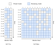
(a) attention head

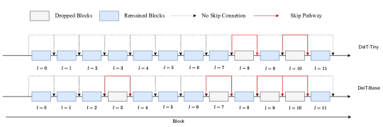
(b) skip connection

Figure 3: Visualizations of: (a) sparse attention head patterns for DeiT-Tiny (left) and DeiT-Base (right); (b) skip connection patterns for DeiT-Tiny (top) and DeiT-Base (bottom).

A.4 Extra results

In this section, we present the result of DeiT with distillation token to extract the best performance vision transformer can reach under UVC framework. Results are shown in 3.

Table 3: Result with distillation token of DeiT

Model	Method	Top-1 Acc. (%)	FLOPs(G)	FLOPs remained(%)
DeiT-Tiny (dist token)	Baseline	74.4	1.3	100
	UVC	74.1(-0.3)	0.66	50.58

References

- Bai et al. (2020) Haoli Bai, Wei Zhang, Lu Hou, Lifeng Shang, Jing Jin, Xin Jiang, Qun Liu, Michael Lyu, and Irwin King. Binarybert: Pushing the limit of bert quantization. arXiv preprint arXiv:2012.15701, 2020.
- Bengio et al. (2013) Yoshua Bengio, Nicholas Léonard, and Aaron Courville. Estimating or propagating gradients through stochastic neurons for conditional computation. arXiv preprint arXiv:1308.3432, 2013.
- Bertasius et al. (2021) Gedas Bertasius, Heng Wang, and Lorenzo Torresani. Is space-time attention all you need for video understanding? arXiv preprint arXiv:2102.05095, 2021.
- Buchbinder & Naor (2009) Niv Buchbinder and Joseph Naor. The design of competitive online algorithms via a primal-dual approach. Now Publishers Inc, 2009.
- Buluc & Gilbert (2008) Aydin Buluc and John R Gilbert. Challenges and advances in parallel sparse matrix-matrix multiplication. In 2008 37th International Conference on Parallel Processing, pp. 503–510. IEEE, 2008.
- Carion et al. (2020) Nicolas Carion, Francisco Massa, Gabriel Synnaeve, Nicolas Usunier, Alexander Kirillov, and Sergey Zagoruyko. End-to-end object detection with transformers. In European Conference on Computer Vision, pp. 213–229. Springer, 2020.
- Chen et al. (2021a) Hanting Chen, Yunhe Wang, Tianyu Guo, Chang Xu, Yiping Deng, Zhenhua Liu, Siwei Ma, Chunjing Xu, Chao Xu, and Wen Gao. Pre-trained image processing transformer. In Proceedings of the IEEE/CVF Conference on Computer Vision and Pattern Recognition, pp. 12299–12310, 2021a.
- Chen et al. (2020a) Mark Chen, Alec Radford, Rewon Child, Jeffrey Wu, Heewoo Jun, David Luan, and Ilya Sutskever. Generative pretraining from pixels. In International Conference on Machine Learning, pp. 1691–1703. PMLR, 2020a.
- Chen et al. (2020b) Tianlong Chen, Jonathan Frankle, Shiyu Chang, Sijia Liu, Yang Zhang, Zhangyang Wang, and Michael Carbin. The lottery ticket hypothesis for pre-trained bert networks. Advances in neural information processing systems, 33:15834–15846, 2020b.
- Chen et al. (2021b) Tianlong Chen, Yu Cheng, Zhe Gan, Lu Yuan, Lei Zhang, and Zhangyang Wang. Chasing sparsity in vision transformers: An end-to-end exploration. arXiv preprint arXiv:2106.04533, 2021b.
- Child et al. (2019) Rewon Child, Scott Gray, Alec Radford, and Ilya Sutskever. Generating long sequences with sparse transformers. arXiv preprint arXiv:1904.10509, 2019.
- Dai et al. (2021) Zhigang Dai, Bolun Cai, Yugeng Lin, and Junying Chen. Up-detr: Unsupervised pre-training for object detection with transformers. In Proceedings of the IEEE/CVF Conference on Computer Vision and Pattern Recognition, pp. 1601–1610, 2021.
- Devlin et al. (2018) Jacob Devlin, Ming-Wei Chang, Kenton Lee, and Kristina Toutanova. Bert: Pre-training of deep bidirectional transformers for language understanding. arXiv preprint arXiv:1810.04805, 2018.
- Dong et al. (2017) Xin Dong, Shangyu Chen, and Sinno Pan. Learning to prune deep neural networks via layer-wise optimal brain surgeon. In Advances in Neural Information Processing Systems, pp. 4857–4867, 2017.
- Dong et al. (2021) Yihe Dong, Jean-Baptiste Cordonnier, and Andreas Loukas. Attention is not all you need: Pure attention loses rank doubly exponentially with depth. arXiv preprint arXiv:2103.03404, 2021.
- Dosovitskiy et al. (2020) Alexey Dosovitskiy, Lucas Beyer, Alexander Kolesnikov, Dirk Weissenborn, Xiaohua Zhai, Thomas Unterthiner, Mostafa Dehghani, Matthias Minderer, Georg Heigold, Sylvain Gelly, et al. An image is worth 16x16 words: Transformers for image recognition at scale. arXiv preprint arXiv:2010.11929, 2020.
- Fan et al. (2019) Angela Fan, Edouard Grave, and Armand Joulin. Reducing transformer depth on demand with structured dropout. arXiv preprint arXiv:1909.11556, 2019.
- Gale et al. (2019) Trevor Gale, Erich Elsen, and Sara Hooker. The state of sparsity in deep neural networks. arXiv preprint arXiv:1902.09574, 2019.
- Ganesh et al. (2020) Prakhar Ganesh, Yao Chen, Xin Lou, Mohammad Ali Khan, Yin Yang, Deming Chen, Marianne Winslett, Hassan Sajjad, and Preslav Nakov. Compressing large-scale transformer-based models: A case study on bert. arXiv preprint arXiv:2002.11985, 2020.
- Gordon et al. (2020) Mitchell A Gordon, Kevin Duh, and Nicholas Andrews. Compressing bert: Studying the effects of weight pruning on transfer learning. arXiv preprint arXiv:2002.08307, 2020.
- Goyal et al. (2020) Saurabh Goyal, Anamitra Roy Choudhury, Saurabh Raje, Venkatesan Chakaravarthy, Yogish Sabharwal, and Ashish Verma. Power-bert: Accelerating bert inference via progressive word-vector elimination. In International Conference on Machine Learning, pp. 3690–3699. PMLR, 2020.
- Guo et al. (2019) Fu-Ming Guo, Sijia Liu, Finlay S Mungall, Xue Lin, and Yanzhi Wang. Reweighted proximal pruning for large-scale language representation. arXiv preprint arXiv:1909.12486, 2019.
- Guo et al. (2021) Yi Guo, Huan Yuan, Jianchao Tan, Zhangyang Wang, Sen Yang, and Ji Liu. Gdp: Stabilized neural network pruning via gates with differentiable polarization. In Proceedings of the IEEE/CVF International Conference on Computer Vision, pp. 5239–5250, 2021.
- Han et al. (2021) Kai Han, Yunhe Wang, Hanting Chen, Xinghao Chen, Jianyuan Guo, Zhenhua Liu, Yehui Tang, An Xiao, Chunjing Xu, Yixing Xu, Zhaohui Yang, Yiman Zhang, and Dacheng Tao. A survey on vision transformer, 2021.
- Han et al. (2015a) Song Han, Huizi Mao, and William J Dally. Deep compression: Compressing deep neural networks with pruning, trained quantization and huffman coding. arXiv preprint arXiv:1510.00149, 2015a.
- Han et al. (2015b) Song Han, Jeff Pool, John Tran, and William Dally. Learning both weights and connections for efficient neural network. In Advances in neural information processing systems, pp. 1135–1143, 2015b.
- He et al. (2016) Kaiming He, Xiangyu Zhang, Shaoqing Ren, and Jian Sun. Deep residual learning for image recognition. In Proceedings of the IEEE conference on computer vision and pattern recognition, pp. 770–778, 2016.
- He et al. (2019) Yang He, Ping Liu, Ziwei Wang, Zhilan Hu, and Yi Yang. Filter pruning via geometric median for deep convolutional neural networks acceleration. In Proceedings of the IEEE Conference on Computer Vision and Pattern Recognition, pp. 4340–4349, 2019.
- He et al. (2017) Yihui He, Xiangyu Zhang, and Jian Sun. Channel pruning for accelerating very deep neural networks. In The IEEE International Conference on Computer Vision (ICCV), Oct 2017.
- He et al. (2018) Yihui He, Ji Lin, Zhijian Liu, Hanrui Wang, Li-Jia Li, and Song Han. Amc: Automl for model compression and acceleration on mobile devices. In Proceedings of the European Conference on Computer Vision (ECCV), pp. 784–800, 2018.
- Hinton et al. (2015) Geoffrey Hinton, Oriol Vinyals, and Jeff Dean. Distilling the knowledge in a neural network. arXiv preprint arXiv:1503.02531, 2015.
- Hou et al. (2020) Lu Hou, Zhiqi Huang, Lifeng Shang, Xin Jiang, Xiao Chen, and Qun Liu. Dynabert: Dynamic bert with adaptive width and depth. arXiv preprint arXiv:2004.04037, 2020.
- Huang et al. (2017) Gao Huang, Zhuang Liu, Laurens Van Der Maaten, and Kilian Q Weinberger. Densely connected convolutional networks. In Proceedings of the IEEE conference on computer vision and pattern recognition, pp. 4700–4708, 2017.
- Jang et al. (2016) Eric Jang, Shixiang Gu, and Ben Poole. Categorical reparameterization with gumbel-softmax. arXiv preprint arXiv:1611.01144, 2016.
- Jia et al. (2021) Ding Jia, Kai Han, Yunhe Wang, Yehui Tang, Jianyuan Guo, Chao Zhang, and Dacheng Tao. Efficient vision transformers via fine-grained manifold distillation. arXiv preprint arXiv:2107.01378, 2021.
- Jiang et al. (2021) Yifan Jiang, Shiyu Chang, and Zhangyang Wang. Transgan: Two pure transformers can make one strong gan, and that can scale up. Advances in Neural Information Processing Systems, 34, 2021.
- Kim et al. (2021) Taehyeon Kim, Jaehoon Oh, NakYil Kim, Sangwook Cho, and Se-Young Yun. Comparing kullback-leibler divergence and mean squared error loss in knowledge distillation. arXiv preprint arXiv:2105.08919, 2021.
- Krizhevsky et al. (2012) Alex Krizhevsky, Ilya Sutskever, and Geoffrey E Hinton. Imagenet classification with deep convolutional neural networks. Advances in neural information processing systems, 25:1097–1105, 2012.
- Lan et al. (2019) Zhenzhong Lan, Mingda Chen, Sebastian Goodman, Kevin Gimpel, Piyush Sharma, and Radu Soricut. Albert: A lite bert for self-supervised learning of language representations. arXiv preprint arXiv:1909.11942, 2019.
- LeCun et al. (1989) Yann LeCun, Bernhard Boser, John S Denker, Donnie Henderson, Richard E Howard, Wayne Hubbard, and Lawrence D Jackel. Backpropagation applied to handwritten zip code recognition. Neural computation, 1(4):541–551, 1989.
- LeCun et al. (1990) Yann LeCun, John S Denker, and Sara A Solla. Optimal brain damage. In Advances in neural information processing systems, pp. 598–605, 1990.
- Lee et al. (2018) Namhoon Lee, Thalaiyasingam Ajanthan, and Philip HS Torr. Snip: Single-shot network pruning based on connection sensitivity. arXiv preprint arXiv:1810.02340, 2018.
- Li et al. (2016) Hao Li, Asim Kadav, Igor Durdanovic, Hanan Samet, and Hans Peter Graf. Pruning filters for efficient convnets. arXiv preprint arXiv:1608.08710, 2016.
- Lin et al. (2020) Mingbao Lin, Rongrong Ji, Yan Wang, Yichen Zhang, Baochang Zhang, Yonghong Tian, and Ling Shao. Hrank: Filter pruning using high-rank feature map. In Proceedings of the IEEE/CVF Conference on Computer Vision and Pattern Recognition, pp. 1529–1538, 2020.
- Lin et al. (2018) Shaohui Lin, Rongrong Ji, Yuchao Li, Yongjian Wu, Feiyue Huang, and Baochang Zhang. Accelerating convolutional networks via global & dynamic filter pruning. In IJCAI, pp. 2425–2432, 2018.
- Liu et al. (2017) Zhuang Liu, Jianguo Li, Zhiqiang Shen, Gao Huang, Shoumeng Yan, and Changshui Zhang. Learning efficient convolutional networks through network slimming. In ICCV, 2017.
- Luo et al. (2017) Jian-Hao Luo, Jianxin Wu, and Weiyao Lin. Thinet: A filter level pruning method for deep neural network compression. In Proceedings of the IEEE international conference on computer vision, pp. 5058–5066, 2017.
- Michel et al. (2019) Paul Michel, Omer Levy, and Graham Neubig. Are sixteen heads really better than one? arXiv preprint arXiv:1905.10650, 2019.
- Mishra & Marr (2018) Asit Mishra and Debbie Marr. Apprentice: Using knowledge distillation techniques to improve low-precision network accuracy. In International Conference on Learning Representations, 2018.
- Pan et al. (2021a) Bowen Pan, Yifan Jiang, Rameswar Panda, Zhangyang Wang, Rogerio Feris, and Aude Oliva. Ia-red2: Interpretability-aware redundancy reduction for vision transformers. arXiv preprint arXiv:2106.12620, 2021a.
- Pan et al. (2021b) Zizheng Pan, Bohan Zhuang, Jing Liu, Haoyu He, and Jianfei Cai. Scalable vision transformers with hierarchical pooling. In Proceedings of the IEEE/CVF International Conference on Computer Vision, pp. 377–386, 2021b.
- Parmar et al. (2018) Niki Parmar, Ashish Vaswani, Jakob Uszkoreit, Lukasz Kaiser, Noam Shazeer, Alexander Ku, and Dustin Tran. Image transformer. In International Conference on Machine Learning, pp. 4055–4064. PMLR, 2018.
- Phang et al. (2021) Jason Phang, Haokun Liu, and Samuel R Bowman. Fine-tuned transformers show clusters of similar representations across layers. arXiv preprint arXiv:2109.08406, 2021.
- Raghu et al. (2021) Maithra Raghu, Thomas Unterthiner, Simon Kornblith, Chiyuan Zhang, and Alexey Dosovitskiy. Do vision transformers see like convolutional neural networks? arXiv preprint arXiv:2108.08810, 2021.
- Sanh et al. (2019) Victor Sanh, Lysandre Debut, Julien Chaumond, and Thomas Wolf. Distilbert, a distilled version of bert: smaller, faster, cheaper and lighter. arXiv preprint arXiv:1910.01108, 2019.
- Shen et al. (2021) Jiayi Shen, Haotao Wang, Shupeng Gui, Jianchao Tan, Zhangyang Wang, and Ji Liu. Umec: Unified model and embedding compression for efficient recommendation systems. In International Conference on Learning Representations, 2021. URL https://openreview.net/forum?id=BM---bH_RSh.
- Tang et al. (2020) Yehui Tang, Yunhe Wang, Yixing Xu, Dacheng Tao, Chunjing Xu, Chao Xu, and Chang Xu. Scop: Scientific control for reliable neural network pruning. arXiv preprint arXiv:2010.10732, 2020.
- Tang et al. (2021) Yehui Tang, Kai Han, Yunhe Wang, Chang Xu, Jianyuan Guo, Chao Xu, and Dacheng Tao. Patch slimming for efficient vision transformers. arXiv preprint arXiv:2106.02852, 2021.
- Tono et al. (2017) Katsuya Tono, Akiko Takeda, and Jun-ya Gotoh. Efficient dc algorithm for constrained sparse optimization. arXiv preprint arXiv:1701.08498, 2017.
- Touvron et al. (2020) Hugo Touvron, Matthieu Cord, Matthijs Douze, Francisco Massa, Alexandre Sablayrolles, and Hervé Jégou. Training data-efficient image transformers & distillation through attention. arXiv preprint arXiv:2012.12877, 2020.
- Vaswani et al. (2017) Ashish Vaswani, Noam Shazeer, Niki Parmar, Jakob Uszkoreit, Llion Jones, Aidan N Gomez, Lukasz Kaiser, and Illia Polosukhin. Attention is all you need. arXiv preprint arXiv:1706.03762, 2017.
- Wang et al. (2021a) Huiyu Wang, Yukun Zhu, Hartwig Adam, Alan Yuille, and Liang-Chieh Chen. Max-deeplab: End-to-end panoptic segmentation with mask transformers. In Proceedings of the IEEE/CVF Conference on Computer Vision and Pattern Recognition, pp. 5463–5474, 2021a.
- Wang et al. (2021b) Yuqing Wang, Zhaoliang Xu, Xinlong Wang, Chunhua Shen, Baoshan Cheng, Hao Shen, and Huaxia Xia. End-to-end video instance segmentation with transformers. In Proceedings of the IEEE/CVF Conference on Computer Vision and Pattern Recognition, pp. 8741–8750, 2021b.
- Wei et al. (2020) Longhui Wei, An Xiao, Lingxi Xie, Xiaopeng Zhang, Xin Chen, and Qi Tian. Circumventing outliers of autoaugment with knowledge distillation. In Computer Vision–ECCV 2020: 16th European Conference, Glasgow, UK, August 23–28, 2020, Proceedings, Part III 16, pp. 608–625. Springer, 2020.
- Xiao et al. (2019) Xia Xiao, Zigeng Wang, and Sanguthevar Rajasekaran. Autoprune: Automatic network pruning by regularizing auxiliary parameters. In Advances in Neural Information Processing Systems, pp. 13681–13691, 2019.
- Xu et al. (2020) Canwen Xu, Wangchunshu Zhou, Tao Ge, Furu Wei, and Ming Zhou. Bert-of-theseus: Compressing bert by progressive module replacing. arXiv preprint arXiv:2002.02925, 2020.
- Yang et al. (2020a) Fuzhi Yang, Huan Yang, Jianlong Fu, Hongtao Lu, and Baining Guo. Learning texture transformer network for image super-resolution. In Proceedings of the IEEE/CVF Conference on Computer Vision and Pattern Recognition, pp. 5791–5800, 2020a.
- Yang et al. (2016) Haichuan Yang, Yijun Huang, Lam Tran, Ji Liu, and Shuai Huang. On benefits of selection diversity via bilevel exclusive sparsity. In Proceedings of the IEEE Conference on Computer Vision and Pattern Recognition, pp. 5945–5954, 2016.
- Yang et al. (2020b) Haichuan Yang, Shupeng Gui, Yuhao Zhu, and Ji Liu. Automatic neural network compression by sparsity-quantization joint learning: A constrained optimization-based approach. In Proceedings of the IEEE/CVF Conference on Computer Vision and Pattern Recognition, pp. 2178–2188, 2020b.
- Yu et al. (2018) Ruichi Yu, Ang Li, Chun-Fu Chen, Jui-Hsin Lai, Vlad I Morariu, Xintong Han, Mingfei Gao, Ching-Yung Lin, and Larry S Davis. Nisp: Pruning networks using neuron importance score propagation. In Proceedings of the IEEE Conference on Computer Vision and Pattern Recognition, pp. 9194–9203, 2018.
- Yu et al. (2021) Shixing Yu, Zhewei Yao, Amir Gholami, Zhen Dong, Michael W Mahoney, and Kurt Keutzer. Hessian-aware pruning and optimal neural implant. arXiv preprint arXiv:2101.08940, 2021.
- Yuan et al. (2020) Li Yuan, Francis EH Tay, Guilin Li, Tao Wang, and Jiashi Feng. Revisiting knowledge distillation via label smoothing regularization. In Proceedings of the IEEE/CVF Conference on Computer Vision and Pattern Recognition, pp. 3903–3911, 2020.
- Yuan et al. (2021) Li Yuan, Yunpeng Chen, Tao Wang, Weihao Yu, Yujun Shi, Zihang Jiang, Francis EH Tay, Jiashi Feng, and Shuicheng Yan. Tokens-to-token vit: Training vision transformers from scratch on imagenet, 2021.
- Zhang & He (2020) Minjia Zhang and Yuxiong He. Accelerating training of transformer-based language models with progressive layer dropping. arXiv preprint arXiv:2010.13369, 2020.
- Zhang et al. (2020) Wei Zhang, Lu Hou, Yichun Yin, Lifeng Shang, Xiao Chen, Xin Jiang, and Qun Liu. Ternarybert: Distillation-aware ultra-low bit bert. arXiv preprint arXiv:2009.12812, 2020.
- Zhao et al. (2020a) Hengshuang Zhao, Li Jiang, Jiaya Jia, Philip Torr, and Vladlen Koltun. Point transformer. arXiv preprint arXiv:2012.09164, 2020a.
- Zhao et al. (2020b) Yang Zhao, Xiaohan Chen, Yue Wang, Chaojian Li, Haoran You, Yonggan Fu, Yuan Xie, Zhangyang Wang, and Yingyan Lin. Smartexchange: Trading higher-cost memory storage/access for lower-cost computation. In 2020 ACM/IEEE 47th Annual International Symposium on Computer Architecture (ISCA), pp. 954–967. IEEE, 2020b.
- Zheng et al. (2020) Minghang Zheng, Peng Gao, Xiaogang Wang, Hongsheng Li, and Hao Dong. End-to-end object detection with adaptive clustering transformer. arXiv preprint arXiv:2011.09315, 2020.
- Zhou et al. (2021) Daquan Zhou, Bingyi Kang, Xiaojie Jin, Linjie Yang, Xiaochen Lian, Zihang Jiang, Qibin Hou, and Jiashi Feng. Deepvit: Towards deeper vision transformer, 2021.
- Zhu et al. (2021) Mingjian Zhu, Kai Han, Yehui Tang, and Yunhe Wang. Visual transformer pruning. arXiv preprint arXiv:2104.08500, 2021.
- Zhu et al. (2020) Xizhou Zhu, Weijie Su, Lewei Lu, Bin Li, Xiaogang Wang, and Jifeng Dai. Deformable detr: Deformable transformers for end-to-end object detection. arXiv preprint arXiv:2010.04159, 2020.