ergm 4: Computational Improvements

Abstract

The ergm package supports the statistical analysis and simulation of network data. It anchors the statnet suite of packages for network analysis in R introduced in a special issue in Journal of Statistical Software in 2008. This article provides an overview of the performance improvements in the 2021 release of ergm version 4. These include performance enhancements to the Markov chain Monte Carlo and maximum likelihood estimation algorithms as well as broader and faster searching for networks with certain target statistics using simulated annealing.

Keywords statnet  $\cdot$ ERGM  $\cdot$ exponential-family random graph models

1 Introduction

The statnet suite of packages for R (R Core Team, 2021) was first introduced in 2008, in volume 24 of Journal of Statistical Software, a special issue devoted to statnet. Together, these packages, which had already gone through the maturing process of multiple releases, provided an integrated framework for the statistical analysis of network data: from data storage and manipulation, to visualization, estimation and simulation. Since that time the existing packages have undergone continual updates to improve and add capabilities, and many new packages have been added to extend the range of network data that can be modeled (e.g., dynamic, valued, sampled, multilevel). It is the ergm package, however, that provides the statistical foundation for all of the other modeling packages in the statnet suite. Version 4 of ergm, released in 2021, is a major upgrade, representing more than a decade of changes and improvements since Hunter et al. (2008). This paper describes updates to the central MCMC and SAN algorithms in the package, demonstrating that these changes have produced substantial improvement in computational speed and efficiency. It is a companion to Krivitsky, Hunter, et al. (2022), which discusses improvements to the user interface and modelling capabilities of ergm.

We repeat the brief presentation from Krivitsky, Hunter, et al. (2022) of the fully general ERGM framework, referring interested readers to Schweinberger et al. (2020) for additional technical details. A random network $\mathbf{Y}$ is distributed according to an ERGM, written $\mathbf{Y}\sim\operatorname{ERGM}_{\mathcal{Y},h,\bm{\eta},\mathbf{g}}({\bm{\theta}})$, if

$$\operatorname{Pr}_{{\bm{\theta}},\mathcal{Y},h,\bm{\eta},\mathbf{g}}(\mathbf{Y}=\mathbf{y})=\frac{h(\mathbf{y})\exp\{\bm{\eta}({\bm{\theta}})^{\top}\mathbf{g}(\mathbf{y})\}}{\kappa_{h,\bm{\eta},\mathbf{g}}({\bm{\theta}},\mathcal{Y})},\ {\mathbf{y}\in\mathcal{Y}}.$$ (1)

In Equation (1), $\mathcal{Y}$ is the sample space of networks; ${\bm{\theta}}$ is a $q$-dimensional parameter vector; $h(\mathbf{y})$ is a reference measure, typically a constant in the case of binary ERGMs; $\bm{\eta}$ is a mapping from ${\bm{\theta}}$ to the $p$-vector of canonical parameters, given by the identity mapping in non-curved ERGMs; $\mathbf{g}$ is a $p$-vector of sufficient statistics; and $\kappa_{h,\bm{\eta},\mathbf{g}}({\bm{\theta}},\mathcal{Y})$ is the normalizer given by $\sum_{{\mathbf{y}^{\prime}\in\mathcal{Y}}}h(\mathbf{y}^{\prime})\exp\{\bm{\eta}({\bm{\theta}})^{\top}\mathbf{g}(\mathbf{y}^{\prime})\}$, which is often intractable for models that seek to reproduce the dependence across ties induced by social effects such as triadic closure. The natural parameter space of the model is $\bm{\Theta}_{\text{N}}\stackrel{{\scriptstyle\text{def}}}{{=}}\{{\bm{\theta}}:\kappa_{h,\bm{\eta},\mathbf{g}}({\bm{\theta}},\mathcal{Y})<\infty\}$.

In the examples throughout the paper we assume that the reader is familiar with the basic syntax and features of ergm included in the 2008 JoSS volume. Where possible we demonstrate new, more general, functionality by comparison, using the old syntax and the new to produce the same result, then moving on with the new syntax to demonstrate the additional utilities.

The source code for the latest development version of the ergm package, along with the LICENSE information under GPL-3, is available at https://github.com/statnet/ergm.

2 Markov chain Monte Carlo enhancements

The simulation of random networks distributed according to a particular ERGM with a known value of the parameter $\bm{\eta}$ is central to nearly all functionality of the ergm package. Clearly, simulation is useful to examine population characteristics of an ERGM using Monte Carlo methods; potentially less obvious is the role that simulation plays in the process of maximum likelihood estimation itself. Markov chain Monte Carlo (MCMC) methods are the means by which ergm implements simulation of networks, and these methods are therefore the workhorses of the package.

2.1 Summary of Metropolis–Hastings algorithms

As explained by Hunter et al. (2008), the goal of MCMC is to create a Markov chain whose stationary distribution is exactly equal to the ERGM with a given value of $\bm{\eta}$. After letting the chain run for a long time, its state may be taken to be an approximate draw from the ERGM in question. The ergm package does this via a Metropolis–Hastings algorithm, a special case of MCMC in which at each iteration, a move from the current network to a new network is proposed according to some probability distribution. The M–H algorithm operates by allowing only two possibilities following this proposal: Either the chain remains at the current network for the next iteration, or the proposed network becomes the current network for the next iteration. The latter possibility occurs with probability

$$\min\left\{1,\frac{\operatorname{Pr}_{{\bm{\theta}},\mathcal{Y},h,\bm{\eta},\mathbf{g}}(\mathbf{Y}=\mathbf{y}^{\text{proposed}})}{\operatorname{Pr}_{{\bm{\theta}},\mathcal{Y},h,\bm{\eta},\mathbf{g}}(\mathbf{Y}=\mathbf{y}^{\text{current}})}\times\frac{q(\mathbf{y}^{\text{current}}\mathop{\,|\,}\nolimits\mathbf{y}^{\text{proposed}})}{q(\mathbf{y}^{\text{proposed}}\mathop{\,|\,}\nolimits\mathbf{y}^{\text{current}})}\right\},$$ (2)

where $q$ denotes the proposal distribution; more specifically, $q({\bf a}\mathop{\,|\,}\nolimits{\bf b})$ is the probability of proposing ${\bf a}$ if the current state is ${\bf b}$.

It is useful to introduce a change statistic or change score

$$\bm{\Delta}_{i,j}\mathbf{g}(\mathbf{y})\stackrel{{\scriptstyle\text{def}}}{{=}}\mathbf{g}[\mathbf{y}\cup\{{(i,j)}\}]-\mathbf{g}[\mathbf{y}\setminus\{{(i,j)}\}],$$ (3)

the effect on the vector of statistics if one were to change the state of the $(i,j)$ relationship from 0 to 1 while holding the rest of the network $\mathbf{y}$ fixed. Let us assume for now that $q$ only allows for changing, or toggling, at most one dyad, which is to say that $q({\bf a}\mathop{\,|\,}\nolimits{\bf b})$ must be zero whenever ${\bf a}$ and ${\bf b}$ differ by more than a single edge. If we call the ratio in Expression (2) the “acceptance ratio,” or AR, then for the proposed toggle of dyad $y_{i,j}$,

$$\log\text{AR}=\pm\bm{\eta}^{\top}\bm{\Delta}_{i,j}\mathbf{g}(\mathbf{y})+\log\frac{q(\mathbf{y}^{\text{current}}\mathop{\,|\,}\nolimits\mathbf{y}^{\text{proposed}})}{q(\mathbf{y}^{\text{proposed}}\mathop{\,|\,}\nolimits\mathbf{y}^{\text{current}})},$$ (4)

where the sign in front of $\bm{\eta}^{\top}\bm{\Delta}_{i,j}\mathbf{g}(\mathbf{y})$ is positive when $y_{i,j}^{\text{proposed}}=1$ and negative when $y_{i,j}^{\text{proposed}}=0$.

It is useful to consider a couple of special cases of the Metropolis–Hastings algorithm (2). When we define $q(\mathbf{y}^{\text{proposed}}\mathop{\,|\,}\nolimits\mathbf{y}^{\text{current}})$ to be proportional to $\operatorname{Pr}_{{\bm{\theta}},\mathcal{Y},h,\bm{\eta},\mathbf{g}}(\mathbf{Y}=\mathbf{y}^{\text{proposed}})$, the value of AR is always 1, which implies that the proposal is always accepted and the resulting algorithm is called full-conditional Gibbs sampling. Another special case is the symmetric proposal, in which $q({\bf a}\mathop{\,|\,}\nolimits{\bf b})=q({\bf b}\mathop{\,|\,}\nolimits{\bf a})$ for all ${\bf a}$ and ${\bf b}$, in which case $\log\mbox{AR}$ is simply $\pm\bm{\eta}\bm{\Delta}_{i,j}\mathbf{g}(\mathbf{y})$. In particular, perhaps the most basic network-based Metropolis–Hastings algorithm for binary networks with $N$ possible edges operates by selecting $\mathbf{y}^{\text{proposed}}$ uniformly from among all $N$ networks that differ from $\mathbf{y}^{\text{current}}$ by exactly one edge toggle; thus, $q(\mathbf{y}^{\text{proposed}}\mathop{\,|\,}\nolimits\mathbf{y}^{\text{current}})$ equals $N^{-1}$ or 0, depending on whether or not $\mathbf{y}^{\text{proposed}}$ and $\mathbf{y}^{\text{current}}$ differ by exactly one toggle.

Simulation of networks from an ERGM using MCMC can be done using simulate, documented at ?simulate.ergm. In place of its original statsonly= argument, simulate methods now take a more versatile output argument, which defaults to "network" for returning a list of generated network objects, "stats" for network statistics, "edgelist" for a more compact representation of the network, or a user-defined function to be evaluated on the sampler state and returned. For example, the following code produces triangle counts for fifty random undirected 10-node networks where each edge occurs independently with probability 2/3. Also, the model statistics—in this case, edge counts—are attached to the result as an attribute "stats":

# Below, we use the fact that logit(2/3) = log(2)

triangles <- function(nwState, ...) summary(as.network(nwState) ~ triangles)

nw10 <- network(10, directed = FALSE)

out <- simulate(nw10 ~ edges, nsim = 50, coef = log(2), output = triangles)

unlist(out, use.names = FALSE)

##  [1] 22 78 41 45 22 50 34 42 42 32 37 48 38 28 65 17 23 29 40 23 66 24 26 39 35 34 33 39 35 39
## [31] 61 27 35 23 32 64 34 20 40 56 30 44 34 36 72 42 30 43 11 32

head(attr(out, "stats"))

##      edges
## [1,]    26
## [2,]    39
## [3,]    32
## [4,]    31
## [5,]    26
## [6,]    33

2.2 MCMC Proposal hints

In Equation (2), basically any proposal distribution $q$ that can, through multiple steps, reach any given point in $\mathcal{Y}$ leads in theory to a Markov chain with the correct stationary distribution. In practice, however, some choices of $q$ may result in rejection of nearly all proposals, a situation informally called “slow mixing.” Thus, it is helpful to have access to different proposals to deploy in different situations.

For example, most real-world social networks are sparse: The vast majority of potential ties are not realized. This results in the basic uniform proposal spending a lot of computing effort proposing toggles to non-edges that are rejected by the Metropolis–Hastings algorithm.

The TNT, or tie/no tie, proposal was introduced in the ergm package specifically to address this slow mixing due to sparsity. TNT proposes a toggle to a uniformly randomly chosen existing edge with probability 1/2, or a toggle to a uniformly randomly chosen dyad—including both edges and non-edges—with probability 1/2. (The description of TNT in Morris et al. (2008) is slightly erroneous; under TNT, the probability of proposing a non-edge for toggling is less than 1/2, not equal to 1/2.) For sparse networks, the set of edges is much smaller than the set of non-edges, so TNT speeds mixing by making many more ‘off’-toggle proposals than would occur if all dyads had the same probability of being proposed for a toggle.

ergm 4 introduces a concept of a hint to enable the user to inform the sampling and estimation algorithm about the properties of the network model that, while they do not affect its stationary distribution, can be helpful in sampling. This information is specified via the MCMC.prop= or obs.MCMC.prop= control parameters as a one-sided formula. For example, MCMC.prop=~sparse (the default) informs the proposal selection algorithm that the sampling should be optimized for sparse networks, which typically means enabling the above-described TNT algorithm. As another example, the code in Section 5 includes the following line within an ergm call:

MCMC.prop = ~strat(attr = ~race, empirical = TRUE) + sparse

The strat hint in this case instructs the proposal distribution to take the race attribute of nodes into account when proposing dyads to toggle; in particular, empirical = TRUE instructs the proposal to weight every possible node-pair race combination according to the proportions of such combinations observed in the network used at the beginning of the Markov chain. Alternatively, the user may pass the strat hint an explicit matrix of weights via the pmat argument. Additional information about hints currently implemented in ergm is available via ? ergmHint, with help("[name]-ergmHint") or ergmHint?[name] for more details about a specific hint.

2.3 MCMC Proposal constraints

It is possible to constrain the sample space of possible networks allowed to have positive probability under the ERGM or, equivalently, to define a subset of networks as having zero probability under the model. Technically, such constraints need not influence our choice of $q$ in Equation (2), since any proposed network whose probability under the model is zero cannot be accepted by the Metropolis–Hastings algorithm. However, in practice it is a waste of computing effort to propose such networks in the first place. The ergm package allows certain types of constraints to be respected by $q$, leading to substantial gains in efficiency when these constraints exist.

The new ergm proposal BDStratTNT, in addition to supporting the strat and sparse hints described in Section 2.2, allows the user to fix edge states of dyads of specified mixing types according to a vertex attribute via the blocks constraint. It also allows for upper bounds on a node’s degree via the bd constraint’s maxout, maxin, and attribs arguments. Documentation for all MCMC proposals visible to ergm is available via ?ergmProposal and, for a specific proposal, help("[name]-ergmProposal") or the shorthand ergmProposal?[name].

In addition, the tergm package includes a generalization of BDStratTNT that specifically supports dynamic models by considering a dyad’s discordance, i.e., whether the dyad is in the same state that it was in at the beginning of the time step when the Markov chain for that step was initialized.

As an example application of the BDStratTNT proposal, the examples of Section 5 contain the following line:

constraints = ~bd(maxout = 1) + blocks(attr = ~sex, levels2 = diag(TRUE, 2))

This line ensures that the sample space of possible networks includes only networks in which no node has a degree of 2 or more—the networks in these examples are undirected—and in which no changes in dyad status between nodes of the same sex value are allowed. These constraints are used to model a network of monogamous heterosexual relationships.

2.4 Adaptive MCMC via effective sample size

ergm 4 implements adaptive MCMC sampling. Monte-Carlo-based approximate maximum likelihood estimation, sometimes abbreviated MCMLE, for an ERGM depends only on the MCMC sample of the sufficient statistic values and is agnostic to the underlying graphs once the statistics have been calculated (Hunter & Handcock, 2006; Krivitsky, 2012; Krivitsky & Butts, 2017). Furthermore, while different algorithms approach the problem in different ways, the estimation ultimately entails matching the mean of the simulated statistic under ${\bm{\theta}}$ to the observed statistic. Thus, the sampling algorithm can focus on obtaining a particular effective sample size of the multivariate sufficient statistic.

The user or the estimation algorithm specifies the target effective sample size, typically via the control parameter MCMC.effectiveSize or, for estimation, MCMLE.effectiveSize, as well as the initial MCMC thinning interval (MCMC.interval) and sample size (MCMC.samplesize). The algorithm then iterates the following steps:

1. Run the Markov chain MCMC.samplesize$\times$MCMC.interval steps forward to obtain an initial sample of size MCMC.samplesize.

2. If the size of the Markov chain’s cumulative sample size exceeds $2\times$MCMC.samplesize, discard every other draw and double MCMC.interval for future runs.

3. Identify a candidate “burn-in” period by fitting a multivariate regression model to the sampled statistics or estimating functions. That is, considering an MCMC sample of $S$ statistics $\mathbf{g}(\mathbf{Y}^{(1)}),\dotsc,\mathbf{g}(\mathbf{Y}^{(S)})$, we find a least-squares fit for

   $$\bm{\eta}^{\prime}({\bm{\theta}})^{\top}\mathbf{g}(\mathbf{Y}^{(s)})=\bm{\beta}_{0}+\bm{\beta}_{1}2^{-s/s_{0}}+\bm{e}^{(s)},\ s=1,\dotsc,S,$$

   where $s_{0}>0$ is the candidate burn-in, $\bm{\beta}_{0},\bm{\beta}_{1}\in\mathbb{R}^{q}$ are (nuisance) parameters, and $\bm{e}^{(s)}\in\mathbb{R}^{q}$ are the residuals. In practice, this estimator can be determined numerically for a given $s_{0}$, so we perform a bisection search over the possible $s_{0}$. Loosely, $s_{0}$ is the number of iterations needed to reduce the expected difference between the current value of the statistic and its equilibrium value by a factor of 2.

4. Evaluate a multivariate extension of the Geweke (1991) convergence diagnostic after discarding sample units up to the estimated $s_{0}$.

5. If nonconvergence is detected, repeat from Step 1, accumulating draws.

6. Calculate the effective sample size of the retained draws using the method of Vats et al. (2019). If satisfied, return.

7. Extrapolate to estimate the additional number of Markov chain steps to obtain the target effective sample size given the current ratio of the sample size to the effective sample size. Advance the estimated number of steps, accumulating draws.

8. Continue from Step 2.

3 Maximum likelihood estimation enhancements

Frequentist inference for ERGMs calls for finding an estimator given observed data on a network or networks, along with estimates of the variability of that estimator that are generally expressed in the form of standard errors. We consider the gold standard of estimation to be the maximum likelihood estimator (MLE), while the maximum pseudo-likelihood estimator (MPLE) is an alternative with certain advantages and disadvantages relative to the MLE. Calculating estimates like these along with their standard errors is the core functionality of the ergm package, and in this section we describe multiple enhancements to the package as of version 4.

The likelihood function is, by definition, the function of Equation (1) when that expression is viewed as a function of ${\bm{\theta}}$. Also in the likelihood function, we often replace the generic $\mathbf{y}$ by $\mathbf{y}^{\text{obs}}$ when an observed network is at hand. The natural logarithm of the likelihood function is often denoted $\ell({\bm{\theta}})$. The MLE $\hat{{\bm{\theta}}}$ is the maximizer of $\ell({\bm{\theta}})$. Alternatively, the MLE is a zero of the gradient of the log-likelihood, also known as the score function (Hunter & Handcock, 2006, Equation 3.1), i.e., $\mathbf{U}(\hat{{\bm{\theta}}})=\operatorname{\mathbf{0}}$, where

$$\mathbf{U}({\bm{\theta}})\stackrel{{\scriptstyle\text{def}}}{{=}}\bm{\nabla}_{{\bm{\theta}}}\ell({\bm{\theta}})=\bm{\eta}^{\prime}({\bm{\theta}})^{\top}[\mathbf{g}(\mathbf{y}^{\text{obs}})-\operatorname{E}_{{\bm{\theta}};\mathcal{Y},h,\bm{\eta},\mathbf{g}}\mathbf{g}(\mathbf{Y})].$$ (5)

The normalizing constant $\kappa_{h,\bm{\eta},\mathbf{g}}({\bm{\theta}},\mathcal{Y})$ of Equation (1) has the property that $\bm{\nabla}_{{\bm{\theta}}}\log\kappa_{h,\bm{\eta},\mathbf{g}}({\bm{\theta}},\mathcal{Y})=\operatorname{E}_{{\bm{\theta}};\mathcal{Y},h,\bm{\eta},\mathbf{g}}\mathbf{g}(\mathbf{Y})$, which gives rise to (5). Often this constant is computationally intractable, and a number of approaches (e.g., Snijders, 2002; Hummel et al., 2012) have been proposed for approximating the MLE. The ergm package defaults to the importance sampling approach of Hunter & Handcock (2006): The likelihood ratio is expressed as an expectation with respect to one of the parameter configurations (that of the $t$th guess, denoted ${\bm{\theta}}^{t}$), and a simulation from that configuration is used to maximize this ratio with respect to ${\bm{\theta}}$ to obtain the next guess ${\bm{\theta}}^{t+1}$. In particular,

$${\bm{\theta}}^{t+1}=\arg\max_{{\bm{\theta}}}\bigg{(}\{\bm{\eta}({\bm{\theta}})-\bm{\eta}({\bm{\theta}}^{t})\}^{\top}\mathbf{g}(\mathbf{y}^{\text{obs}})-\log\frac{1}{S}\sum_{s=1}^{S}\exp[\{\bm{\eta}({\bm{\theta}})-\bm{\eta}({\bm{\theta}}^{t})\}^{\top}\mathbf{g}(\mathbf{y}^{{\bm{\theta}}^{t},s})]\bigg{)},$$ (6)

where $\mathbf{y}^{{\bm{\theta}}^{t},1},\ldots,\mathbf{y}^{{\bm{\theta}}^{t},S}$ is an approximate sample from $\operatorname{Pr}_{{\bm{\theta}}^{t};\mathcal{Y},h,\bm{\eta},\mathbf{g}}$ obtained via MCMC. It is because an MCMC-generated sample is used to obtain an approximate MLE that this and related procedures are sometimes called MCMCMLE; the fact that this approach is a central pillar of ergm underscores how integral the MCMC algorithms are to nearly all facets of the package.

3.1 Missing data

Handcock (2003) observed that for a non-curved family, i.e., where $\bm{\eta}({\bm{\theta}})\equiv{\bm{\theta}}$, there is no maximizer in Equation (6) if $\mathbf{g}(\mathbf{y}^{\text{obs}})$ is not in the convex hull of the sample $\mathbf{g}(\mathbf{y}^{{\bm{\theta}}^{t},s})$. This can be seen because if $\mathbf{g}(\mathbf{y}^{\text{obs}})$ is outside of the convex hull, then one can increase the maximand arbitrarily by selecting ${\bm{\theta}}^{\prime}=\alpha\mathbf{g}(\mathbf{y}^{\text{obs}})+{\bm{\theta}}^{t}$ with $\alpha\to\infty$: the first term in (6) would grow faster than any summand or combination of summands of the second. Conversely, if $\mathbf{g}(\mathbf{y}^{\text{obs}})$ is in the interior of the convex hull, then for any direction for ${\bm{\theta}}^{\prime}$, some combinations of summands would grow faster than the first term. Hummel et al. (2012) therefore proposed to translate $\mathbf{g}(\mathbf{y}^{\text{obs}})$ in the direction of the centroid of $\mathbf{g}(\mathbf{y}^{{\bm{\theta}}^{t},s})$ until it is sufficiently deep inside the convex hull, making an update that would be guaranteed to be a unique maximizer in the correct general direction. Krivitsky (2017) extended this approach to curved ERGMs.

When there are missing data or an observation process, as described in Section 7 of Krivitsky, Hunter, et al. (2022), the form of the maximand becomes

$$\log\frac{1}{S}\sum_{s=1}^{S}\exp[\{\bm{\eta}({\bm{\theta}}^{\prime})-\bm{\eta}({\bm{\theta}}^{t})\}^{\top}\mathbf{g}(\mathbf{y}^{{\bm{\theta}}^{t},s}|\mathbf{y}^{\text{obs}})]-\log\frac{1}{S}\sum_{s=1}^{S}\exp[\{\bm{\eta}({\bm{\theta}}^{\prime})-\bm{\eta}({\bm{\theta}}^{t})\}^{\top}\mathbf{g}(\mathbf{y}^{{\bm{\theta}}^{t},s})],$$

where $\mathbf{y}^{{\bm{\theta}}^{t},s}|\mathbf{y}^{\text{obs}}$ are draws from the distribution $\operatorname{ERGM}_{\mathcal{Y}(\mathbf{y}^{\text{obs}})}({\bm{\theta}}^{t})$. This expression can be maximized to infinity if any of $\mathbf{g}(\mathbf{y}^{{\bm{\theta}}^{t},s}|\mathbf{y}^{\text{obs}})$ is outside of the convex hull of $\mathbf{g}(\mathbf{y}^{{\bm{\theta}}^{t},s})$, as that summand could then dominate all others in both summations.

ergm therefore scales all $\mathbf{g}(\mathbf{y}^{{\bm{\theta}}^{t},s}|\mathbf{y}^{\text{obs}})$ toward the centroid of $\mathbf{g}(\mathbf{y}^{{\bm{\theta}}^{t},s})$ until they are all sufficiently deep in the convex hull. That they are being scaled towards a point guarantees that such a scaling factor exists, unless the rank of $\mathbf{y}^{{\bm{\theta}}^{t},s}|\mathbf{y}^{\text{obs}}$ is higher than that of $\mathbf{g}(\mathbf{y}^{{\bm{\theta}}^{t},s})$. Version 4 of the ergm package introduces substantial improvements to the algorithm that determines whether a point is inside the convex hull of a given set of points. For instance, the algorithm now returns, after solving a single linear program, the exact multiplier that scales the point so that it lies on the boundary of the convex hull; furthermore, ergm now uses the Rglpk package rather than the lpSolveAPI package when the former is installed, which according to our tests solves the convex hull linear program substantially more efficiently. Further details of the improvements to the convex hull algorithm are in Krivitsky, Kuvelkar, et al. (2022).

3.2 Standard errors for maximum pseudo-likelihood estimation

To define the maximum pseudo-likelihood estimator (MPLE) for a binary network, we must first define the pseudo-likelihood function. To this end, let us consider that Equation (4) arises due to the fact that under the ERGM of Equation (1),

$$\log\frac{\operatorname{Pr}_{{\bm{\theta}},\mathcal{Y},h,\bm{\eta},\mathbf{g}}(\mathbf{y}\cup\{{(i,j)}\})}{\operatorname{Pr}_{{\bm{\theta}},\mathcal{Y},h,\bm{\eta},\mathbf{g}}(\mathbf{y}\setminus\{{(i,j)}\})}=\log\frac{\operatorname{Pr}_{{\bm{\theta}},\mathcal{Y},h,\bm{\eta},\mathbf{g}}(Y\!_{i,j}=1\,|\,\mathbf{y}_{ij}^{c})}{\operatorname{Pr}_{{\bm{\theta}},\mathcal{Y},h,\bm{\eta},\mathbf{g}}(Y\!_{i,j}=0\,|\,\mathbf{y}_{ij}^{c})}=\bm{\eta}^{\top}\bm{\Delta}_{i,j}\mathbf{g}(\mathbf{y}),$$ (7)

where $\mathbf{y}_{ij}^{c}$ is the entirety of $\mathbf{y}$ except $y_{i,j}$. If we imagine that all $Y\!_{i,j}$ are mutually independent Bernoulli random variables with distributions given by (7)—i.e., that $\operatorname{logit}\operatorname{Pr}_{{\bm{\theta}},\mathcal{Y},h,\bm{\eta},\mathbf{g}}(Y\!_{i,j}=1)=\bm{\eta}^{\top}\bm{\Delta}_{i,j}\mathbf{g}(\mathbf{y})$—then multiplying their individual probability mass functions gives a function called the pseudo-likelihood, whose maximizer is known as the maximum pseudo-likelihood estimator (MPLE).

As discussed in Hunter et al. (2008), the ergm function uses logistic regression to obtain MPLEs in non-curved models. The glm function in R returns not only estimated logistic regression coefficients (parameters) but also standard errors for those coefficients. Earlier versions of ergm had simply reported these standard errors without modification whenever the user asked for MPLE model output; however, these standard errors are inaccurate when the edges are not independent. Indeed, a straightforward Taylor approximation (Schmid & Hunter, 2021) gives

$$\operatorname{var}_{{\bm{\theta}};\mathcal{Y},h,\bm{\eta},\mathbf{g}}(\hat{{\bm{\theta}}}_{\text{MPLE}})\approx[J({\bm{\theta}})]^{-1}\operatorname{var}_{{\bm{\theta}};\mathcal{Y},h,\bm{\eta},\mathbf{g}}({\mathbf{U}}({\bm{\theta}}))[J({\bm{\theta}})]^{-1},$$ (8)

where we assume that the ERGM with parameter ${\bm{\theta}}$ is the true model for the distribution that gave rise to the observed network and $J({\bm{\theta}})$ is the negative Hessian of the logarithm of the pseudo-likelihood function. Since ${\bm{\theta}}$ is of course unknown, in practice we may approximate the right hand side above by substituting $\hat{{\bm{\theta}}}_{\text{MPLE}}$ for ${\bm{\theta}}$.

Whenever the form of $\mathbf{g}(\mathbf{y})$ results in all $Y\!_{i,j}$ being mutually independent, as discussed in Krivitsky, Hunter, et al. (2022), the MPLE equals the MLE. This also implies $J({\bm{\theta}})=\operatorname{var}_{{\bm{\theta}};\mathcal{Y},h,\bm{\eta},\mathbf{g}}[{\mathbf{U}}({\bm{\theta}})]$ for all ${\bm{\theta}}$, so the expression on the right hand side simplifies to $[J({\bm{\theta}})]^{-1}$. Indeed, the standard errors returned by the logistic regression algorithm are those given by $[J(\hat{{\bm{\theta}}}_{\text{MPLE}})]^{-1}$. Yet for non-dyad-independent models, these logistic-regression-based standard errors are poor approximations to the true standard deviations of the parameter estimates. The ergm package therefore implements the technique described by Schmid & Hunter (2021), using (8) with $\hat{{\bm{\theta}}}_{\text{MPLE}}$ in place of ${\bm{\theta}}$ to provide standard errors. For this purpose, the middle term must be estimated by the sample covariance matrix from a random sample obtained using Markov chain Monte Carlo with $\hat{{\bm{\theta}}}_{\text{MPLE}}$ as the true parameter value. Alternatively, ergm can approximate MPLE standard errors via a bootstrap method, as proposed by Schmid & Desmarais (2017).

Logistic regression to obtain the MPLE is performed automatically when estimate="MPLE" is used with the ergm function. The ergm package also provides a function ergmMPLE that produces the response vector and predictor matrix that may be used, for instance, to produce the logistic regression output directly via the glm function in R. The ergmMPLE function gives its output in the form of weighted response/predictor combinations, weighted according to their multiplicity, in order to conserve memory in cases where particular combinations occur frequently.

data(g4)

print(lr <- ergmMPLE(g4 ~ edges + triangle))

## $response
## [1] 0 0 0 1 1 1
##
## $predictor
##      edges triangle
## [1,]     1        1
## [2,]     1        0
## [3,]     1        2
## [4,]     1        0
## [5,]     1        1
## [6,]     1        2
##
## $weights
## [1] 2 1 4 1 2 2

The weights vector sums to $4\times 3$, the number of potential relations in the network. We may verify that the MPLE obtained via ergm matches direct logistic regression estimates:

rbind(coef(ergm(g4~edges + triangle, estimate="MPLE")),

  coef(glm(response ~ predictor - 1, weights  = weights, data = lr, family = "binomial")))

##          edges   triangle
## [1,] 0.2057346 -0.4114692
## [2,] 0.2057346 -0.4114692

The predictor vector associated with dyad $(i,j)$ is the change statistic vector for that dyad under the model, and the change statistics can be queried directly to produce an array of change statistics corresponding to each tail, head, and statistic combination using the output="array" argument:

ergmMPLE(g4 ~ edges + triangle, output = "array")$predictor

## , , term = edges
##
##     head
## tail V1 V2 V3 V4
##   V1 NA  1  1  1
##   V2  1 NA  1  1
##   V3  1  1 NA  1
##   V4  1  1  1 NA
##
## , , term = triangle
##
##     head
## tail V1 V2 V3 V4
##   V1 NA  0  1  2
##   V2  0 NA  2  1
##   V3  1  2 NA  2
##   V4  2  1  2 NA

Alternatively output="dyadlist" produces an uncompressed list:

ergmMPLE(g4 ~ edges + triangle, output = "dyadlist")$predictor

##       tail head edges triangle
##  [1,]    1    2     1        0
##  [2,]    1    3     1        1
##  [3,]    1    4     1        2
##  [4,]    2    1     1        0
##  [5,]    2    3     1        2
##  [6,]    2    4     1        1
##  [7,]    3    1     1        1
##  [8,]    3    2     1        2
##  [9,]    3    4     1        2
## [10,]    4    1     1        2
## [11,]    4    2     1        1
## [12,]    4    3     1        2

3.3 Log-likelihood estimation

Likelihood-based estimation relies not only on the value of the maximizer $\hat{{\bm{\theta}}}$ of the log-likelihood function, but also on the maximum value $\ell(\hat{{\bm{\theta}}})$ that function obtains. Model selection criteria such as AIC and BIC are based on this maximized log-likelihood—they are equal to $-2\ell(\hat{{\bm{\theta}}})+2p$ and $-2\ell(\hat{{\bm{\theta}}})+p\log d$, respectively, where $p$ is the number of model parameters and $d$ is the number of observed, non-fixed potential relations in the network—as are the standard chi-squared tests based on drop-in-deviance.

Hunter & Handcock (2006) point out that the null deviance, which is equal to $-2\ell(\operatorname{\mathbf{0}})$, is straightforward to calculate; in the case of binary networks, it equals $2N\log 2$, where again $N$ is the number of observed, non-fixed potential edges. Yet log-likelihood values are sometimes computationally intractable, as mentioned in Section 1. A novel method currently employed by the ergm package is to first identify all dyadic dependent terms in the model, then find the MLE and corresponding log-likelihood value in the constrained parameter space that fixes the values of the coefficients corresponding to those terms at zero. This calculation is straightforward using logistic regression, as explained in Section 3.2. If we denote the MLE of this sub-model as $\tilde{{\bm{\theta}}}$, then our task becomes estimation of $\ell(\hat{{\bm{\theta}}})-\ell(\tilde{{\bm{\theta}}})$, since the second term in this expression is known from logistic regression output.

Section 5 of Hunter & Handcock (2006) addresses the problem of likelihood ratio testing, which on the logarithmic scale is exactly the problem of calculating the difference of two log-likelihoods such as $\ell(\hat{{\bm{\theta}}})-\ell(\tilde{{\bm{\theta}}})$. That paper describes the idea of path sampling (Gelman & Meng, 1998), which is based on the following observation: if we define a smooth path in parameter space from $\tilde{{\bm{\theta}}}$ to $\hat{{\bm{\theta}}}$, that is, a differentiable function $\mathbf{m}$ that maps the closed unit interval $[0,1]$ into the parameter space so that $\mathbf{m}(0)=\tilde{{\bm{\theta}}}$ and $\mathbf{m}(1)=\hat{{\bm{\theta}}}$, then

$$\log\kappa_{h,\bm{\eta},\mathbf{g}}(\hat{{\bm{\theta}}},\mathcal{Y})-\log\kappa_{h,\bm{\eta},\mathbf{g}}(\tilde{{\bm{\theta}}},\mathcal{Y})=\int_{0}^{1}\operatorname{E}_{\mathbf{m}(u);\mathcal{Y},h,\bm{\eta},\mathbf{g}}\left\{{\frac{d}{du}}\bm{\eta}[\mathbf{m}(u)]\right\}^{\top}\mathbf{g}(\mathbf{Y})\,du$$ (9)

by the fundamental theorem of calculus, where $\kappa_{h,\bm{\eta},\mathbf{g}}({\bm{\theta}},\mathcal{Y})$ is the normalizing constant of Equation (1). Pulling the expectation and differentiation operators outside of the integral, the expression remaining under the integral sign is also an expectation with respect to a random variable $U$ uniformly distributed on $(0,1)$. Thus, Equation (9) implies that

$$\log\kappa_{h,\bm{\eta},\mathbf{g}}(\hat{{\bm{\theta}}},\mathcal{Y})-\log\kappa_{h,\bm{\eta},\mathbf{g}}(\tilde{{\bm{\theta}}},\mathcal{Y})=\operatorname{E}_{\mathcal{Y},h,\bm{\eta},\mathbf{g}}\left\{\frac{d}{dU}\bm{\eta}[\mathbf{m}(U)]\right\}^{\top}\mathbf{g}(\mathbf{Y}),$$ (10)

where the expectation is taken with respect to the joint distribution of $U$ and $\mathbf{Y}$, where $U\sim\operatorname{Unif}(0,1)$ and $\mathbf{Y}\mathop{\,|\,}\nolimits U$ is distributed according to the ERGM of Equation (1) with parameter $\mathbf{m}(U)$. Here, we introduce a shifted version of the vector $\mathbf{g}(\cdot)$ of sufficient statistics,

$$\bm{z}(\mathbf{y})\stackrel{{\scriptstyle\text{def}}}{{=}}\mathbf{g}(\mathbf{y})-\mathbf{g}(\mathbf{y}^{\text{obs}}),$$

where if missing data are present we replace $\mathbf{g}(\mathbf{y}^{\text{obs}})$ by $\operatorname{E}_{{\bm{\theta}};\mathcal{Y},h,\bm{\eta},\mathbf{g}}\mathbf{g}(\mathbf{Y}\mathop{\,|\,}\nolimits\mathbf{y}^{\text{obs}})$; yet here we assume for simplicity of notation that $\bm{z}(\mathbf{y})$ does not depend on ${\bm{\theta}}$. If $\bm{z}(\cdot)$ is substituted for $\mathbf{g}(\cdot)$, then $\ell({\bm{\theta}})=-\log\kappa_{h,\bm{\eta},\bm{z}}({\bm{\theta}},\mathcal{Y})$, so for instance Equation (10) gives a convenient expression for $\ell(\tilde{{\bm{\theta}}})-\ell(\hat{{\bm{\theta}}})$.

In practice, the problem with Equation (10) is that simulating the first network $\mathbf{Y}$ from a given parameter configuration ${\bm{\theta}}=\mathbf{m}(U)$ requires a long “burn-in” period, which makes the direct approach of drawing a $U_{k}$ then a $\mathbf{Y}_{k}|U_{k}$ for $k=1,\dotsc,K$ impractical. On the other hand, once “burned in,” subsequent draws $\mathbf{Y}_{2},\dotsc,\mathbf{Y}_{K}$ from the same distribution cost relatively little additional effort. For this reason, the ergm package currently implements a technique known as bridge sampling (Meng & Wong, 1996) as an approximation of Equation (10).

Bridge sampling in ergm partitions the unit interval into $J$ sub-intervals, each of length $1/J$, where $u_{j}$ is taken to be the center of the $j$th sub-interval for $j=1,\dotsc,J$. For each $j$, we simulate a random sample $\mathbf{Y}_{j1},\ldots,\mathbf{Y}_{jK}$ of networks from the ERGM with parameter $\mathbf{m}(u_{j})$. Since the $u_{j}$ values may be viewed as a rough approximation of a uniform sample on $[0,1]$, the idea of Equation (10) leads to

$$\ell(\hat{{\bm{\theta}}})-\ell(\tilde{{\bm{\theta}}})\approx-\frac{1}{JK}\sum_{j=1}^{J}\sum_{k=1}^{K}\nabla\mathbf{m}(u_{j})\nabla\bm{\eta}[\mathbf{m}(u_{j})]\bm{z}(\mathbf{Y}_{jk}).$$ (11)

(The analogous Equation 5.4 of Hunter & Handcock (2006) omits the needed factor $-1/J$.)

Equation (11) entails two different approximations of Equation 10: One in approximating the expectation of $\mathbf{Y}$ using simulated networks and one in approximating the $\operatorname{Unif}(0,1)$ distribution by $u_{0},\ldots,u_{J}$. The first of these is due to Monte Carlo error, so it may be quantified; this is the source of the standard errors reported for AIC and BIC for dyadic-dependent models. The user can specify a control parameter bridge.target.se, via control.logLik.ergm() or snctrl(), to continue bridge sampling at values $u_{l,j}$ for $j=1,\dotsc,J$ and $l=1,2,\dotsc$ ad infinitum, until the estimated standard error due to the first approximation is below it.

The second approximation leads to a bias even in the idealized case where $K\to\infty$, which only vanishes as $J\to\infty$. Our experiments suggest that this bias is small, but in the adaptive mode triggered by bridge.target.se, it is addressed by shifting each series of $J$ points by a value from a low-discrepancy sequence in one dimension: $u_{l,j}=(j-1/2+v_{l})/J$, for $v_{l}=\operatorname{mod}((l-1)/\phi+1/2,1)-1/2$, a shifted Kronecker sequence with $v_{1}=0$ and the inverse of the Golden Ratio $\phi$ as its coefficient. The “weight” of each $u_{l,j}$ in Equation 11 is then adjusted to be proportional to the size of its Voronoi cell, which is the length of the region of points on the unit interval that are nearer to $u_{l,j}$ than to any other point $u_{l^{\prime},j^{\prime}}$ sampled so far.

As a further optimization, the algorithm reduces the need for burning-in by reordering points $u_{l,j}$ for a given $l$ such that $u_{l+1,1}$ is as close to $u_{l,J}$ as possible, $u_{l+1,2}$ to $u_{l+1,1}$, and so on.

3.4 Curved MPLE and curved ERGMs as “first-class” models

Curved ERGMs—those for which $\bm{\eta}({\bm{\theta}})\neq{\bm{\theta}}$—were introduced by Hunter & Handcock (2006) to facilitate estimation of the decay parameter in the geometrically-weighted triadic degree and triadic terms. They stated a score function for such models and outlined an MCMLE algorithm that could be used to update ${\bm{\theta}}$ given a sample of sufficient statistics from the previous guess.

However, the implementation prior to ergm 4 was incomplete in the following respect: While it could estimate curved ERGMs, it required the end-user to specify the initial values for their parameters. This is because maximum pseudo-likelihood estimation (MPLE) for curved models had not been derived and implemented. Non-MCMLE methods did not support curved ERGMs at all.

The score function for the curved ERGM MPLE was derived by Krivitsky (2017) and is implemented in ergm 4. Thus, to fit a curved model with geometrically weighted degree, one previously had to specify an initial value, as in:

data(florentine)

ergm(flomarriage ~ edges + gwdegree(0.25))  # Initial guess for the decay parameter = 0.25

Now, the initial value is determined automatically if we simply specify

data(florentine)

ergm(flomarriage ~ edges + gwdegree)

##
## Call:
## ergm(formula = flomarriage ~ edges + gwdegree)
##
## Last MCMC sample of size 486 based on:
##          edges        gwdegree  gwdegree.decay
##        -1.5334         -0.1318          0.6730
##
## Monte Carlo Maximum Likelihood Coefficients:
##          edges        gwdegree  gwdegree.decay
##     -1.6255705      -0.0008501       0.2259348

In situations where the decay parameter is fixed and known, its value may be specified directly or via the partial offset capability, also new in ergm 4. Thus, the two ergm calls below are equivalent, though their coefficient estimates differ slightly because the fitting algorithm is stochastic:

data(sampson)

coef(ergm(samplike~edges+gwesp(0.25, fix=TRUE), control=snctrl(MCMLE.maxit=2)))

##            edges gwesp.fixed.0.25
##       -1.6374758        0.4136882

coef(ergm(samplike~edges+offset(gwesp(), c(FALSE,TRUE)), offset.coef=0.25,

          control=snctrl(MCMLE.maxit=2)))

##               edges               gwesp offset(gwesp.decay)
##          -1.6152582           0.4011794           0.2500000

3.5 Contrastive Divergence

Contrastive divergence (CD) is a technique taken from the computer science literature and proposed in the context of ERGMs by Asuncion et al. (2010). Much more detail about its use for ERGMs is provided by Krivitsky (2017). Essentially, CD provides a spectrum of estimation algorithms with MPLE at one extreme and MLE at the other. Little is presently known about the efficacy of algorithms lying between these two extremes.

The ergm package implements CD estimates, which may be obtained by passing estimate="CD" to the ergm function. Since not much is known about the quality of these estimates, their most promising use at present is as starting values for MCMC-based maximum likelihood estimation as described at the beginning of Section 3; that is, they are used for the initial guess ${\bm{\theta}}^{t}$ for $t=0$. By default, they are used where available implementations of MPLE are inapplicable, in particular valued ERGMs or binary ERGMs with dyad-dependent sample space constraints: unlike MPLE, which must be rederived for each reference distribution and sample space constraint, contrastive divergence can reuse the proposals from the MCMC implementation (Krivitsky, 2017).

3.6 Confidence stopping criterion

The ergm package implements several methods to determine when to declare convergence in an MCMLE algorithm and report the results. They are selected via the MCMLE.termination parameter as follows:

MCMLE.termination="Hotelling"

Convergence is declared if an autocorrelation-adjusted Hotelling $T^{2}$ test is unable to reject the null hypothesis that the estimating function equals zero, which for non-curved models on fully observed networks means simply that the expected value of the simulated statistic equals the observed statistic at a high level ($\alpha=0.5$ by default). Krivitsky (2017) provides additional details.

MCMLE.termination="Hummel"

The algorithm of Hummel et al. (2012) is used: Convergence is declared if for two consecutive parameter updates, the observed statistic is sufficiently deep in the interior of the convex hull of the sample of simulated statistics. (For curved models, sample values of estimating functions are used instead.) However, this criterion can be problematic for partially observed networks, as it requires that every point in the constrained (conditional) sample be in the interior of the convex hull of the unconstrained sample, which can be problematic when the fraction of the missing dyads and the dimension of the parameter vector are moderately high.

MCMLE.termination="confidence"

Loosely based on the algorithms of Vats et al. (2019), this method, which is the default in ergm 4, implements a form of equivalence testing. The general idea of equivalence testing is to define the null hypothesis to be that the difference between the observed and the expected statistics large enough to be interesting. Thus, rejecting the null hypothesis entails deciding that the difference is small enough that convergence is declared.

4 Simulated Annealing

ergm has enhanced its flexibility in the use of simulated annealing (SAN) to randomly generate networks with a particular set of network statistics. This capability is used by the package in the process of finding an MLE, particularly when estimating from sufficient statistics alone rather than an entire network. At least some of the methods enabled by SAN are the subject of ongoing research. For instance, Schmid & Hunter (2020) find that SAN can be used to find effective starting values for the iterative algorithm described at the beginning of Section 3. The rest of this section describes simulated annealing and details some of its capabilities and uses within the ergm package.

4.1 Formulation of SAN algorithm

Let $\mathbf{g}$ be a vector of target statistics for the network we wish to construct. That is, we are given an arbitrary network $\mathbf{y}^{0}\in\mathcal{Y}$, and we seek a network $\mathbf{y}\in\mathcal{Y}$ such that $\mathbf{g}(\mathbf{y})\approx\mathbf{g}$—ideally equality is achieved, but in practice we may have to settle for a close approximation. The variant of simulated annealing used in ergm is as follows.

The energy function is defined $E_{W}(\mathbf{y})=\{\mathbf{g}(\mathbf{y})-\mathbf{g}\}^{\top}W\{\mathbf{g}(\mathbf{y})-\mathbf{g}\}$, with $W$ a symmetric positive (barring multicollinearity in statistics) definite matrix of weights. This function achieves 0 only if the target is reached. A good choice of this matrix yields a more efficient search.

A standard simulated annealing loop is used, as described below, with some modifications. In particular, we allow the user to specify a vector of offsets $\bm{\eta}$ to bias the annealing, with $\eta_{k}=0$ denoting no offset. As illustrated in the example below, offsets can be used with SAN to forbid certain statistics from ever increasing or decreasing. As with ergm, offset terms are specified using the offset() decorator and their coefficients specified with the offset.coef argument. By default, finite offsets are ignored by, but this can be overridden by setting the control argument SAN.ignore.finite.offsets = FALSE.

The number of simulated annealing runs is specified by the SAN.maxit control parameter and the initial value of the temperature $T$ is set to SAN.tau. The value of $T$ decreases linearly until $T=0$ at the last run, which implies that all proposals that increase $E_{W}(\mathbf{y})$ are rejected. The weight matrix $W$ is initially set to $I_{p}/p$, where $I_{p}$ is the identity matrix of an appropriate dimension.

For weight $W$ and temperature $T$, the simulated annealing iteration proceeds as follows:

1. Test if $E_{W}(\mathbf{y})=0$. If so, then exit.

2. Generate a perturbed network $\mathbf{y}^{\star}$ from a proposal that respects the model constraints. (This is typically the same proposal as that used for MCMC.)

3. Store the quantity $\mathbf{g}(\mathbf{y}^{\star})-\mathbf{g}(\mathbf{y})$ for later use.

4. Calculate acceptance probability

   $$\alpha=\exp[-\{E_{W}(\mathbf{y}^{\star})-E_{W}(\mathbf{y})\}/T+\bm{\eta}^{\top}\{\mathbf{g}(\mathbf{y}^{\star})-\mathbf{g}(\mathbf{y})\}].$$

   (If $\lvert\eta_{k}\rvert=\infty$ and $g_{k}(\mathbf{y}^{\star})-g_{k}(\mathbf{y})=0$, their product is defined to be $0$.)

5. Replace $\mathbf{y}$ with $\mathbf{y}^{\star}$ with probability $\min(1,\alpha)$.

After the specified number of iterations, $T$ is updated as described above, and $W$ is recalculated by first computing a matrix $S$, the sample covariance matrix of the proposed differences stored in Step 3 (i.e., whether or not they were rejected), then $W=S^{+}/\operatorname{tr}(S^{+})$, where $S^{+}$ is the Moore–Penrose pseudoinverse of $S$. The differences in Step 3 closely reflect the relative variances and correlations among the network statistics.

In Step 2, the many options for MCMC proposals, including those newly added to the ergm package as covered in Section 5.1, can provide for effective means of speeding the SAN algorithm’s search for a viable network. This phenomenon is illustrated in Section 5.3.

The example below illustrates the use of offsets in a 100-node network in which each node has a sex attribute with possible values "M" and "F". Suppose that we wish to construct a network with 30 edges in which no edges are allowed between nodes of the same sex value, nor that result in any node having more than one edge—constraints that would arise, for example, if we wished to model a network of heterosexual, monogamous relationships. SAN can find such a network by placing offset parameters valued at -Inf on ERGM terms corresponding to nodematch("sex") and concurrent:

nw <- network.initialize(100, directed = FALSE)

nw %v% "sex" <- rep(c("M","F"), 50)

example <- san(nw ~ edges + offset(nodematch("sex")) + offset(concurrent),

               offset.coef = c(-Inf, -Inf), target.stats = 30)

summary(example ~ edges + nodematch("sex") + concurrent)

##         edges nodematch.sex    concurrent
##            30             0             0

The output of the summary function above verifies that the constraints are satisfied by the generated network example.

5 Computing efficiency tests on large networks

Version 4 of the ergm package enables substantial gains in computing efficiency relative to earlier versions of the packages. There are many reasons for these gains, including better algorithms (e.g., improvements to simulated annealing and maximum pseudo-likelihood estimation), better use of parallelism, and new MCMC proposals. As pointed out elsewhere, improved MCMC proposals lead to performance improvements across a wide range of ergm package functionality due to the pervasive use of simulation in the ergm workflow. Where these improvements have greatest impact, we see speedups of as much as two orders of magnitude for comparable computing tasks. This section highlights some of the key changes and demonstrates their impacts, using in some cases networks with one million nodes.

The code used to produce the results in each subsection of Section 5 is given in that subsection. Each test is based on a hypothetical network constructed from the cohab dataset in the ergm package, where the nodes are persons and the edges represent cohabiting pairs. The distribution of nodal attributes and edges is based on aggregated statistics from the National Survey of Family Growth (NSFG) (National Center for Health Statistics, 2020). The nodes have demographic attributes—sex, age, and race/ethnicity/immigration status—sampled using the NSFG post-stratification weights that have been adjusted to match the demographics of King County in Washington State. The edges represent heterosexual cohabitation relationships observed in the data, which imposes two constraints on the network that we can exploit for computing efficiency gains: the networks are bipartite, i.e., only edges between male and female nodes are allowed, and nodal degree is capped at one. In addition to demographic attributes, the test dataset includes two more nodal variables as distributed in the adjusted NSFG data: sexual identity and whether the node has at least one persistent non-cohabiting partner. The data and model are a simplified version of an actual applied research project that models the spread of HIV. Additional information about these data are available by typing help(cohab).

5.1 Impact of new proposals on Markov chain mixing

This section examines the evolution of a Markov chain based on a particular ERGM for a million-node network whose nodal covariates are based on the demographic statistics of the cohab dataset. The Markov chain is initialized at an empty network, i.e., one with no edges, and we compare the approach of the ERGM statistics to a set of target values using each of three different proposals. Again, these target values are based on the cohab dataset. The model has 15 statistics, defined by the formula used for the simulation:

data(cohab)

CohabFormula <-

  nw ~ edges + nodefactor("sex.ident", levels = 3) + nodecov("age") + nodecov("agesq") +

       nodefactor("race", levels = -5) + nodefactor("othr.net.deg", levels = -1) +

       nodematch("race", diff = TRUE) + absdiff("sqrt.age.adj")

Additionally, as explained above, constraints are imposed to prevent edges between nodes with the same sex attribute and also to prevent concurrent partnerships, so a node’s degree in this network can be only 0 or 1.

The code below prepares the simulation by estimating ERGM parameters for a network of 50,000 nodes that give mean statistics equal to the target statistics based on data collected in King County.

net_size <- 50000

set.seed(0)

inds <- sample(seq_len(NROW(cohab_PopWts)), net_size, TRUE, cohab_PopWts$weight)

if(RunMode != "Skip") {

  nw <- network.initialize(net_size, directed = FALSE)

  set.vertex.attribute(nw, names(cohab_PopWts)[-1], cohab_PopWts[inds,-1])

  fit <- ergm(nw ~ edges + nodefactor("sex.ident", levels = 3) + nodecov("age") + nodecov("agesq") +

                   nodefactor("race", levels = -5) + nodefactor("othr.net.deg", levels = -1) +

                   nodematch("race", diff = TRUE) + absdiff("sqrt.age.adj") +

                   offset(nodematch("sex", diff = FALSE)) + offset(concurrent),

                   target.stats = cohab_TargetStats,

                   offset.coef = c(-Inf, -Inf),

                   eval.loglik = FALSE,

                   constraints = ~bd(maxout = 1) + blocks(attr = ~sex, levels2 = diag(TRUE, 2)),

                   control = snctrl(MCMC.prop = ~strat(attr = ~race, empirical = TRUE) + sparse,

                                    init.method = "MPLE", init.MPLE.samplesize = 5e7,

                                    MPLE.constraints.ignore = TRUE, MCMLE.effectiveSize = NULL,

                                    MCMC.burnin = 5e4, MCMC.interval = 5e4, MCMC.samplesize = 7500,

                                    parallel = ncores, SAN.nsteps = 5e7,

                                    SAN.prop=~strat(attr = ~race, pmat = cohab_MixMat) + sparse))

  el <- do.call(rbind, lapply(fit$newnetworks, as.edgelist))

  attrs <- cbind(nw %v% "race", nw %v% "age")

  colnames(attrs) <- c("race", "age")

  tailattrs <- attrs[el[,1],]

  headattrs <- attrs[el[,2],]

  attrnames <- "race"

  levs <- sort(unique(apply(attrs[,attrnames,drop=FALSE], 1, paste, collapse = ".")))

  tails <- factor(apply(tailattrs[,attrnames,drop=FALSE], 1, paste, collapse = "."), levels = levs)

  heads <- factor(apply(headattrs[,attrnames,drop=FALSE], 1, paste, collapse = "."), levels = levs)

  mmr <- table(from = tails, to = heads)

  mmr <- mmr + t(mmr) - diag(diag(mmr))

  attrnames <- c("race", "age")

  levs <- sort(unique(apply(attrs[,attrnames,drop=FALSE], 1, paste, collapse = ".")))

  tails <- factor(apply(tailattrs[,attrnames,drop=FALSE], 1, paste, collapse = "."), levels = levs)

  heads <- factor(apply(headattrs[,attrnames,drop=FALSE], 1, paste, collapse = "."), levels = levs)

  mmra <- table(from = tails, to = heads)

  mmra <- mmra + t(mmra) - diag(diag(mmra))

  mmra[mmra == 0] <- 1/2 ## ensure positive proposal weight for all allowed pairings

}

The next block of code initializes a Markov chain at an empty million-node network and tests three different Metropolis–Hastings proposals, each with equilibrium distribution given by the ERGM corresponding to the estimated coefficients from above, adjusted as needed for a network 20 times as large as the network used above. This code is written to exploit parallel computing and can take a while to execute, depending on the value of nsim, the required number of simulated vectors of statistics which, when multiplied by interval, gives the total number of Metropolis–Hastings proposals in each Markov chain.

multiplier <- 20

if (RunMode != "Skip") {

  library(parallel)

  nw <- network.initialize(net_size * multiplier, directed = FALSE)

  indsLong <- rep(inds, length.out = net_size * multiplier)

  set.vertex.attribute(nw, names(cohab_PopWts)[-1], cohab_PopWts[indsLong,-1])

  coef <- coef(fit)[seq_len(length(coef(fit)) - 2)]

  coef[1] <- coef[1] - log(multiplier)

  TargetStatsLarge <- cohab_TargetStats * multiplier

  attribs <- matrix(FALSE, nrow = network.size(nw), ncol = 2)

  attribs[nw %v% "sex" == "M", 1] <- TRUE

  attribs[nw %v% "sex" == "F", 2] <- TRUE

  maxout <- matrix(0, nrow = network.size(nw), ncol = 2)

  maxout[nw %v% "sex" == "M", 2] <- 1

  maxout[nw %v% "sex" == "F", 1] <- 1

  Constraints1 <- list("TNT"~bd(attribs = attribs, maxout = maxout),

                   ~bd(maxout = 1) + blocks(attr = "sex", levels2 = diag(TRUE, 2))

                   + strat(attr = ~paste(race, sep = "."), pmat = mmr),

                   ~bd(maxout = 1) + blocks(attr = "sex", levels2 = diag(TRUE, 2))

                   + strat(attr = ~paste(race, age, sep = "."), pmat = mmra))

  ConstraintNames1 <- c("\"TNT\"~bd(sex,1)", "~bd(1)+blocks(sex)+strat(race)",

                 "~bd(1)+blocks(sex)+strat(race,age)")

  nsim <- ifelse(RunMode =="Large", 1e5, 50)

  interval <- 1e6

  run_simulate <- function(constraint) {

    library(ergm)

    elapsed <- system.time ({

      x <- simulate(CohabFormula, coef = coef, constraints = constraint, output = "stats",

                  nsim = nsim, control = snctrl(MCMC.interval = interval, MCMC.burnin = interval))

    })

    x <- matrix(c(x), nrow = nsim, dimnames = dimnames(x))

    list(statsmatrix = x, elapsed=elapsed)

  }

  cl <- makeCluster(length(Constraints1))

  clusterExport(cl, "nw")

  clusterExport(cl, "CohabFormula")

  clusterExport(cl, "coef")

  clusterExport(cl, "mmr")

  clusterExport(cl, "mmra")

  clusterExport(cl, "nsim")

  clusterExport(cl, "interval")

  clusterExport(cl, "attribs")

  clusterExport(cl, "maxout")

  rv <- clusterApply(cl, Constraints1, run_simulate)

  stopCluster(cl)

  z1 <- lapply(rv, `[[`, "statsmatrix")

  times1 <- lapply(rv, `[[`, "elapsed")

}

The trace plots of Figure 1 show how the Markov chain, starting from the empty network, evolves as a function of the total number of proposals made. Only four of the fifteen ERGM statistics are depicted to save space, and the horizontal axis starts at 3 becuase statistics are sampled only every 1000 proposals. We see that all four of the statistics depicted have stabilized at their target values after roughly $10^{7}$ proposals using the BDStratTNT proposal stratified on both race and age. On the other hand, TNT without any stratification has not yet converged to the target values after $10^{9}$ proposals; in longer tests, we find that even after $10^{11}$ proposals the nodematch.race.B statistic has not quite achieved the target value using TNT.

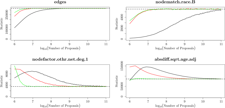
Figure 1: Approach to equilibrium of Markov chains using TNT (black), BDStratTNT stratified only on race (red), and BDStratTNT stratified jointly on race and age (green). Target values are shown as horizontal dotted lines.

Figure 1 shows that the BDStratTNT proposal stratifying on only race holds roughly an order of magnitude advantage over TNT for three of the four statistics shown, and this advantage increases to 3 or more orders of magnitude for the statistic representing homophily for race group B (nodematch.race.B). The BDStratTNT proposal stratifying on both race and age roughly matches the performance of the race-only stratification for the statistics representing density (edges) and homophily for race group B, but it does significantly better for the terms representing the effects of age differences (absdiff.sqrt.age.adj) and having at least one persistent relationship in another network (nodefactor.othr.net.deg.1).

The faster convergence of the absdiff.sqrt.age.adj statistic when the proposal considers stratification by age is expected, since the model favors ties on dyads where the nodes have similar ages and such dyads will have toggles proposed more frequently when proposals are stratified according to age mixing.

There is a modest sex asymmetry in the age mixing, with females tending to be about 1.5 years younger than their male partners; however, taking this asymmetry into account in the proposal stratification via the pmat argument of the strat hint does not produce significant additional gains. The faster convergence of nodefactor.othr.net.deg.1 may arise because nodes having positive othr.net.deg tend to be younger than the population average age, so proposal age stratification can hasten equilibration of the nodefactor.othr.net.deg.1 statistic.

5.2 Gains in Effective Sample Size

This section compares Markov chains based on effective sample size (ESS), as calculated by the coda package (Plummer et al., 2006), for the 15 individual statistics of the ERGM of Section 5.1. The network in these tests has 50,000 nodes, and the Markov chains are sampled every 100 proposals until a total of 500,000 vectors of statistics are produced. (In longer runs, we have generated 10 million vectors per chain.) ESS gives a way to compare various Markov chains that all have the same equilibrium distribution, since chains that do not mix well do not produce samples that vary much, which in turn reduces their ESS.

Among the Metropolis–Hastings algorithms we test, some stratify the nodes by the race variable when proposing node pairs to toggle. We may use the pmat argument to explicitly pass a matrix of probabilities that the algorithm should assign to each possible combination of levels of race, and in our tests we use two versions of this pmat argument. The first, called mmr, simply assigns probabilities based on the edge fractions observed in the cohab dataset. The second, called mmr_mod, gives more weight, in selecting potential MCMC edge toggles, to smaller race groups than their edge fraction would dictate: Finally, the mmra matrix, used for the proposal that stratifies by both race and age, simply uses the observed edge fractions for each stratum.

if (RunMode != "Skip") {

  mmr_mod <- mmr

  mmr_mod[-(4:5),] <- mmr_mod[,-(4:5)]*sqrt(6)

  mmr_mod[,-(4:5)] <- mmr_mod[-(4:5),]*sqrt(6)

  mmr_mod[3,] <- mmr_mod[3,]*sqrt(2)

  mmr_mod[,3] <- mmr_mod[,3]*sqrt(2)

  mmr_mod[4,] <- 1.5*mmr_mod[4,]

  mmr_mod[,4] <- 1.5*mmr_mod[,4]

}

Now that the network and all necessary supporting objects are in place, we can run the test. The value of nsimESS gives the number of 15-dimensional vectors of statistics, sampled once every 100 proposals according to the value of interval, produced before the Markov chain is stopped.

nsimESS <- ifelse(RunMode =="Small", 1e5, 1e7)

intervalESS <- 100

if (RunMode != "Skip") {

  nw <- fit$newnetworks[[1]] # Use network from previous 50000-node fit

  coef <- coef(fit)[seq_len(length(coef(fit)) - 2)] # Use estimates from previous fit

#  save(nw, coef, file="nwANDcoef.RData")

#}

  attribs <- matrix(FALSE, nrow = network.size(nw), ncol = 2)

  attribs[nw %v% "sex" == "M", 1] <- TRUE

  attribs[nw %v% "sex" == "F", 2] <- TRUE

  maxout <- matrix(0, nrow = network.size(nw), ncol = 2)

  maxout[nw %v% "sex" == "M", 2] <- 1

  maxout[nw %v% "sex" == "F", 1] <- 1

  Constraints2 <- list("TNT"~bd(attribs = attribs, maxout = maxout),

                 ~bd(maxout = 1) + blocks(attr = "sex", levels2 = diag(TRUE, 2)),

                 ~bd(maxout = 1) + blocks(attr = "sex", levels2 = diag(TRUE, 2))

                                 + strat(attr = ~paste(race, sep = "."), pmat = mmr),

                 ~bd(maxout = 1) + blocks(attr = "sex", levels2 = diag(TRUE, 2))

                                 + strat(attr = ~paste(race, sep = "."), pmat = mmr_mod),

                 ~bd(maxout = 1) + blocks(attr = "sex", levels2 = diag(TRUE, 2))

                                 + strat(attr = ~paste(race, age, sep = "."), pmat = mmra))

  ConstraintNames2 <- c("\"TNT\"~bd(sex,1)",

               "~bd(1)+blocks(sex)",

               "~bd(1)+blocks(sex)+strat(race)",

               "~bd(1)+blocks(sex)+strat(race.mod)",

               "~bd(1)+blocks(sex)+strat(race,age)")

  set.seed(0)

  z2 <- matrix(0, 5, 15)

  rownames(z2) <- ConstraintNames2

  times2 <- list()

  for(i in seq_along(Constraints2)) {

    times2[[i]] <- system.time({

        x <- simulate(CohabFormula,

                  coef = coef,

                  constraints = Constraints2[[i]],

                  nsim = nsimESS,

                  output = "stats",

                  control = snctrl(MCMC.interval = intervalESS,

                                   MCMC.burnin = intervalESS))

    z2[i,] <- coda::effectiveSize(x)

    })

  }

}

The first column in Table 1 indicates, in abbreviated form, the hints and/or constraints that were specified, in addition to the default sparse hint used for all rows. Thus, the first row uses the TNT proposal, while all other rows use BDStratTNT with varying levels of complexity in the hints and constraints passed to the proposal.

Table 1: Effective sample sizes for 4 of the 15 statistics from an MCMC sample of size 1e+07 with interval 100 using the hints and constraints shown in the leftmost column in addition to the sparse hint, which is used in all cases.

	edges	race B homoph.	other net deg. 1+	$\sqrt{\text{age diff.}}$
"TNT" bd(sex,1)	2862.0	207.8	5495.6	2149.4
bd(1)+blocks(sex)	25720.3	1016.7	10671.4	12228.1
bd(1)+blocks(sex)+strat(race)	27421.0	4336.6	11706.8	13732.8
bd(1)+blocks(sex)+strat(race.mod)	20206.4	12715.2	10565.9	10360.8
bd(1)+blocks(sex)+strat(race,age)	28086.4	4941.7	15569.6	6892.2

Of the proposals tested, only TNT was available in ergm prior to version 3.10. The various versions of the BDStratTNT proposal all produce larger ESS values for every statistic measured. If we compare the first row of Table 1 with, say, the fourth row, representing the BDStratTNT proposal that stratifies on the modified race effect and respects the heterosexual nature of the model and the bound placed on degree—no node is ever allowed to have more than one tie—we see that the smallest value in row 4, 570.4, is roughly 70 times as large as the smallest value in row 1, 8.2. Indeed, these two ESS values are the smallest in their respective rows across all fifteen statistics:

min(z2[4, ])/min(z2[1, ])

## [1] 95.2256

Since different proposals require different computing effort, we may also compare the proposals by dividing ESS by the total time required. Table 2 summarizes these ESS per minute measurements. Comparing rows 1 and 4 as before, we see that the improvement in minimum ESS per minute across all 15 statistics is roughly 86-fold.

Table 2: Effective sample sizes per minute for 4 of the 15 statistics from an MCMC sample of size 1e+07 with interval 100 using the hints and constraints shown in the leftmost column in addition to the sparse hint, which is used in all cases.

	edges	race B homoph.	other net deg. 1+	$\sqrt{\text{age diff.}}$
"TNT" bd(sex,1)	310.2	22.5	595.7	233.0
bd(1)+blocks(sex)	3397.2	134.3	1409.5	1615.1
bd(1)+blocks(sex)+strat(race)	3401.1	537.9	1452.0	1703.3
bd(1)+blocks(sex)+strat(race.mod)	2461.8	1549.2	1287.3	1262.3
bd(1)+blocks(sex)+strat(race,age)	2185.4	384.5	1211.5	536.3

5.3 Impact of MCMC improvements on simulated annealing speed

The trace plots in Figure 2 show how various statistics approach their target values during a run of ergm’s simulated annealing algorithm, starting from an empty million-node network, with each of three different proposals. The horizontal axis is the base 10 logarithm of the number of proposals made, and the vertical axis is the statistic value, with the target value indicated as the horizontal purple line. Statistics are sampled every 1000 proposals, so the horizontal axis starts at 3. The SAN run takes place at a fixed temperature of 0, with the matrix of weights being the diagonal matrix of reciprocal squared target statistics divided by their sum. This choice of temperature and weight matrix settings was made to try to minimize the effect of these choices on the algorithm’s behavior and thereby isolate the different effects of the proposals, yet we find that using the default TNT settings explained in Section 4.1 leads to similar behavior to that reported in Figure 2.

Figure 2 shows that the BDStratTNT proposal stratifying on only race yields an advantage of roughly 1 to 2 orders of magnitude over TNT for these statistics, with the BDStratTNT proposal stratifying on both race and age yielding an additional half an order of magnitude or less. Here is the code used to produce the figure:

if (RunMode != "Skip") {

  library(parallel)

  set.seed(0)

  nw <- network.initialize(net_size * multiplier, directed = FALSE)

  set.vertex.attribute(nw, names(cohab_PopWts)[-1], cohab_PopWts[indsLong,-1])

  attribs <- matrix(FALSE, nrow = network.size(nw), ncol = 2)

  attribs[nw %v% "sex" == "M", 1] <- TRUE

  attribs[nw %v% "sex" == "F", 2] <- TRUE

  maxout <- matrix(0, nrow = network.size(nw), ncol = 2)

  maxout[nw %v% "sex" == "M", 2] <- 1

  maxout[nw %v% "sex" == "F", 1] <- 1

  samplesize <- ifelse(RunMode  =="Large", 1e6, 5e4)

  nsteps <- ifelse(RunMode  =="Large", 1e9, 5e7)

  invcov <- diag(1/(TargetStatsLarge**2))

  invcov <- invcov/sum(invcov)

  run_san <- function(constraint) {

    library(ergm)

    elapsed <- system.time({

      rv <- san(CohabFormula,

              constraints = constraint,

              target.stats = TargetStatsLarge,

              control = snctrl(SAN.maxit = 1,

                               SAN.invcov = invcov,

                               SAN.nsteps = nsteps,

                               SAN.samplesize = samplesize))

    })

    sm <- attr(rv, "stats")

    sm <- t(t(sm) + TargetStatsLarge)

    list(statsmatrix = sm, elapsed = elapsed)

  }

  cl <- makeCluster(length(Constraints1))

  clusterExport(cl, "CohabFormula")

  clusterExport(cl, "nw")

  clusterExport(cl, "mmr")

  clusterExport(cl, "mmra")

  clusterExport(cl, "samplesize")

  clusterExport(cl, "nsteps")

  clusterExport(cl, "invcov")

  clusterExport(cl, "TargetStatsLarge")

  clusterExport(cl, "attribs")

  clusterExport(cl, "maxout")

  rv <- clusterApply(cl, Constraints1, run_san)

  stopCluster(cl)

  z3 <- lapply(rv, `[[`, "statsmatrix")

  times3 <- lapply(rv, `[[`, "elapsed")

}

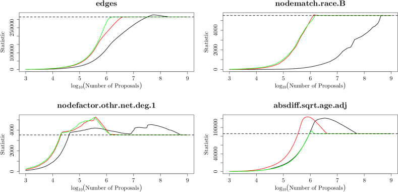
Figure 2: Approach to target values of SAN runs using proposals TNT (black), BDStratTNT stratified only on race (red), and BDStratTNT stratified jointly on race and age (green). Target values are shown as horizontal lines.

5.4 Impact of MCMC improvements on estimation time

The cumulative effect of the myriad improvements to the computing machinery of the ergm package are perhaps best appreciated by comparing version 4 with earlier versions of the package. Table 3 shows computing times for fitting the model described in Section 5.1 to a network with 50,000 nodes. The two versions of ergm are the latest version 4 as well as version 3.10, which may be obtained from CRAN archives. While version 3.10 was released in 2019 and is therefore quite a bit more recent than the version (2.1) that was published along with Hunter et al. (2008), the efficiency improvements are nonetheless substantial for this particular model-fitting example.

For the MCMC proposals, the version 4 runs use BDStratTNT, while the proposals that allow for stratification while taking bounded degree constraints into account were not available for version 3.10; thus, the 3.10 runs use plain TNT. All the runs enforce network constraints via offset terms with coefficients set to $-\infty$ when maximizing the pseudolikelihood, as the MPLE procedure cannot handle such constraints. The “3.10 without bd” fits also utilize these offsets to enforce constraints during MCMC, while the offsets are redundant in MCMC for the “3.10 with bd” and version 4 fits. An important difference between “3.10 with bd” and version 4, which also uses bd, is the implementation of bd: in ergm 3.10, the only bd implementation available was a rejection algorithm, while in ergm 4, the BDStratTNT proposal maintains the necessary state to avoid the need for a rejection algorithm when imposing upper bounds on degree.

In this particular model, we have a target mean degree of about 0.63, meaning that approximately 86% of randomly chosen dyads cannot be toggled without violating the degree bound when the network is near equilibrium. Of the 14% that can, half cannot be toggled due to the heterosexuality constraint, which is also taken into account by BDStratTNT. The BDStratTNT proposal is thus naively about 15 times as efficient for this model as a proposal that does not constructively take the constraints into account. The stratification of proposals by race, also handled by BDStratTNT, yields still further improvement. This expected baseline increase in efficiency, together with the effective sample size results described in 5.2, explains the choice of fixed interval values 1/20 as large in the third row of Table 3 as in the first two rows. The rightmost column of Table 3 uses adaptive MCMC to fit the model, which is new in ergm 4 and is the default. One may disable adaptive MCMC by setting MCMLE.effectiveSize = NULL.

All fits reported in the table parallelize MCMC using an iMac with 6 cores, so improvements in parallelization between ergm versions 3.10 and 4 are also represented in Table 3.

A few words are in order regarding the bd constraint and its relationship with simulated annealing in earlier versions of ergm. As mentioned above, it is possible to enforce a constraint such as a bound on degree without using bd by adding an offset term to the model, say, degree(k) where k is one larger than the maximum allowable degree, and fixing its coefficient value at -Inf. However, offsets were previously ignored by san, the simulated annealing function used to produce an initial network, potentially resulting in an initial network not satisfying the constraints. This in turn could produce a poor initial parameter value, as obtained from the MPLE of the network generated by san. Indeed, we see in the first row of Table 3 that models fit in 3.10 without using bd produce much longer fit times for this particular model. The san function now respects offsets, but the facts that multiple algorithms in ergm might rely on constraints and not all such algorithms currently optimize their treatment of both offsets and explicit constraints lead us to recommend the redundancy in specifying such constraints.

First, we present the code used to test version 4. There is no "Small" option for the tests in this subsection; using RunMode=="Small" employs the results from a previously saved run, whereas RunMode=="Large" takes a very long time, possibly several days, to finish.

if (RunMode == "Large") { # There is no "Small" option here; "Small" works like "Skip"

  net_size <- 5e4

  V4Times <- list()

  reps <- ifelse(RunMode =="Large", 5, 1)

  for(i in seq_len(reps)) { # number of repetitions

    set.seed(i)

    for (j in 1:3) { # first two nonadaptive; third adaptive

      nw <- network.initialize(net_size, directed = FALSE)

      inds <- sample(seq_len(NROW(cohab_PopWts)), net_size, TRUE, cohab_PopWts$weight)

      set.vertex.attribute(nw, names(cohab_PopWts)[-1], cohab_PopWts[inds,-1])

      elapsed <- system.time({

        interval <- 500*10^j; if (j==3) interval <- NULL

        samplesize <- 7500; if (j==3) samplesize <- NULL

        effectiveSize <- 64; if (j<3) effectiveSize <- NULL

        fit <- ergm(nw ~ edges +

                    nodefactor("sex.ident", levels = 3) +

                    nodecov("age") +

                    nodecov("agesq") +

                    nodefactor("race", levels = -5) +

                    nodefactor("othr.net.deg", levels = -1) +

                    nodematch("race", diff = TRUE) +

                    absdiff("sqrt.age.adj") +

                    offset(nodematch("sex", diff = FALSE)) +

                    offset(concurrent),

                    target.stats = cohab_TargetStats,

                    offset.coef = c(-Inf, -Inf),

                    eval.loglik = FALSE,

                    constraints = ~bd(maxout = 1) + blocks(attr = ~sex, levels2 = diag(TRUE, 2)),

                    control = snctrl(MCMC.prop = ~strat(attr = ~race, empirical = TRUE) + sparse,

                                     init.method = "MPLE",

                                     init.MPLE.samplesize = 5e7,

                                     MPLE.constraints.ignore = TRUE,

                                     MCMLE.effectiveSize = effectiveSize,

                                     MCMC.burnin = interval,

                                     MCMC.interval = interval,

                                     MCMC.samplesize = samplesize,

                                     parallel = ncores,

                                     SAN.nsteps = 5e7,

                                     SAN.prop=~strat(attr = ~race, pmat = cohab_MixMat) + sparse))

      })

      V4Times[[j + (i-1)*3]] <- elapsed[3] # save elapsed time

    }

  }

}

To test ergm version 3.10, we use the callr package to open a new R process, install the older version of ergm along with the related packages statnet.common and network, and run a lengthy example in the new process. To run this code requires the installation of the dplyr and lpSolve packages, which were dependencies of ergm 3.10, along with the callr package.

Version3Code <- function(cohab_PopWts, cohab_TargetStats, ncores) {

  # First, install older versions of three packages including ergm 3.10 to current dir

  archv <- "https://cran.r-project.org/src/contrib/Archive/"

  install.packages(paste(archv, "statnet.common/statnet.common_4.3.0.tar.gz", sep=""),

                   repos = NULL, type = "source", lib=".")

  library(statnet.common, lib=".")

  install.packages(paste(archv, "network/network_1.15.tar.gz", sep=""),

                   repos = NULL, type = "source", lib=".")

  library(network, lib=".")

  install.packages(paste(archv, "ergm/ergm_3.10.4.tar.gz", sep=""),

                   repos = NULL, type = "source", lib=".")

  library(ergm, lib=".")

  net_size <- 5e4

  set.seed(1)

  nw <- network.initialize(net_size, directed = FALSE)

  inds <- sample(seq_len(NROW(cohab_PopWts)), net_size, TRUE, cohab_PopWts$weight)

  set.vertex.attribute(nw, names(cohab_PopWts)[-1], cohab_PopWts[inds,-1])

  attrib_mat <- matrix(FALSE, nrow = net_size, ncol = 2)

  attrib_mat[nw %v% "sex" == "F", 1] <- TRUE

  attrib_mat[nw %v% "sex" == "M", 2] <- TRUE

  maxout_mat <- matrix(0, nrow = net_size, ncol = 2)

  maxout_mat[nw %v% "sex" == "F", 2] <- 1

  maxout_mat[nw %v% "sex" == "M", 1] <- 1

  V3Times <- list()

  trial <- 1

  for(interval in c(1e5, 1e6)) {

  # calculate fit without bounded degree contraints

    elapsed <- system.time ({

      fit <- ergm(nw ~ edges +

                   nodefactor("sex.ident", levels = 3) +

                   nodecov("age") +

                   nodecov("agesq") +

                   nodefactor("race", levels = -5) +

                   nodefactor("othr.net.deg", levels = -1) +

                   nodematch("race", diff = TRUE) +

                   absdiff("sqrt.age.adj") +

                   offset(nodematch("sex", diff = FALSE)) +

                   offset(concurrent),

                   target.stats = cohab_TargetStats,

                   offset.coef = c(-Inf, -Inf),

                   eval.loglik = FALSE,

                   control = control.ergm(init.method = "MPLE",

                                          MCMC.burnin = interval,

                                          MCMC.interval = interval,

                                          MCMC.samplesize = 7500,

                                          parallel = ncores,

                                          MCMLE.maxit = 1000,

                                          MCMLE.termination = "none",

                                          SAN.control = control.san(SAN.nsteps = 1e4)))

    })

    V3Times[[trial]] <- elapsed[3]

    trial <- trial + 1

    # calculate fit with bounded degree contraints

    elapsed <- system.time({

      fit <- ergm(nw ~ edges +

                   nodefactor("sex.ident", levels = 3) +

                   nodecov("age") +

                   nodecov("agesq") +

                   nodefactor("race", levels = -5) +

                   nodefactor("othr.net.deg", levels = -1) +

                   nodematch("race", diff = TRUE) +

                   absdiff("sqrt.age.adj") +

                   offset(nodematch("sex", diff = FALSE)) +

                   offset(concurrent),

                   target.stats = cohab_TargetStats,

                   offset.coef = c(-Inf, -Inf),

                   eval.loglik = FALSE,

                   constraints = ~bd(attribs = attrib_mat, maxout = maxout_mat),

                   control = control.ergm(init.method = "MPLE",

                                          MCMC.burnin = interval,

                                          MCMC.interval = interval,

                                          MCMC.samplesize = 7500,

                                          parallel = ncores,

                                          MCMLE.maxit = 1000,

                                          MCMLE.termination = "none",

                                          SAN.control = control.san(SAN.nsteps = 1e4)))

    })

    V3Times[[trial]] <- elapsed[3] # save elapsed time

    trial <- trial + 1;

  }

  V3Times

}

if (RunMode == "Large") { # There is no "Small" option here; "Small" works like "Skip"

  library(dplyr) # Both dplyr and lpSolve are dependencies of ergm 3.10

  library(lpSolve)

  library(callr)

  V3Times <- r(Version3Code, args=list(cohab_PopWts=cohab_PopWts,

                                       cohab_TargetStats=cohab_TargetStats, ncores=ncores))

}

Table 3: Model fit times for various ergm versions and settings using fixed short, fixed long, and adaptive MCMC intervals.

	Short	Long	Adaptive
3.10 without bd	22.64 hours (1e5 interval)	4.41 hours (1e6 interval)	N/A
3.10 with bd	5.72 hours (1e5 interval)	1.3 hours (1e6 interval)	N/A
4.1	281.5 seconds (5e3 interval)	658.2 seconds (5e4 interval)	569 seconds

6 Discussion

This paper describes and tests the many changes in the ergm package since version 2.1 was released concurrently with Hunter et al. (2008) that influence the computing efficiency of the various Monte Carlo-based algorithms upon which it depends. Among other things, we demonstrate that the computing algorithms have improved by up to several orders of magnitude; coupled with the concomitant increase of processor speed, these developments enable ergm users to model networks of a size that was infeasible a decade ago. Furthermore, ergm the many related packages in the statnet suite for R (R Core Team, 2021) are undergoing continual development, and we intend that this trend will continue.

References

Asuncion, A., Liu, Q., Ihler, A., & Smyth, P. (2010). Learning with blocks: Composite likelihood and contrastive divergence. In Y. W. Teh & M. Titterington (Eds.), Proceedings of the thirteenth international conference on artificial intelligence and statistics (Vol. 9, pp. 33–40). PMLR. http://proceedings.mlr.press/v9/asuncion10a.html

R Core Team. (2021). R: A language and environment for statistical computing. R Foundation for Statistical Computing. http://www.R-project.org/

Gelman, A., & Meng, X.-L. (1998). Simulating normalizing constants: From importance sampling to bridge sampling to path sampling. Statistical Science, 13, 163–185.

Geweke, J. (1991). Bayesian statistics 4 (J. M. Bernado, J. O. Berger, A. P. Dawid, & A. F. M. Smith, Eds.). Federal Reserve Bank of Minneapolis, Research Department Minneapolis, MN, USA.

Handcock, M. S. (2003). Assessing degeneracy in statistical models of social networks. University of Washington. https://csss.uw.edu/files/working-papers/2003/wp39.pdf

Hummel, R. M., Hunter, D. R., & Handcock, M. S. (2012). Improving simulation-based algorithms for fitting ERGMs. Journal of Computational and Graphical Statistics, 21(4), 920–939. https://doi.org/10.1080/10618600.2012.679224

Hunter, D. R., & Handcock, M. S. (2006). Inference in curved exponential family models for networks. Journal of Computational and Graphical Statistics, 15(3), 565–583. https://doi.org/10.1198/106186006x133069

Hunter, D. R., Handcock, M. S., Butts, C. T., Goodreau, S. M., & Morris, M. (2008). ergm: A package to fit, simulate and diagnose exponential-family models for networks. Journal of Statistical Software, 24(3), 1–29. https://doi.org/10.18637/jss.v024.i03

Krivitsky, P. N. (2012). Exponential-family random graph models for valued networks. Electronic Journal of Statistics, 6, 1100–1128. https://doi.org/10.1214/12-EJS696

Krivitsky, P. N. (2017). Using contrastive divergence to seed Monte Carlo MLE for exponential-family random graph models. Computational Statistics & Data Analysis, 107, 149–161. https://doi.org/10.1016/j.csda.2016.10.015

Krivitsky, P. N., & Butts, C. T. (2017). Exponential-family random graph models for rank-order relational data. Sociological Methodology, 47(1), 68–112. https://doi.org/10.1177/0081175017692623

Krivitsky, P. N., Hunter, D. R., Morris, M., & Klumb, C. (2022). ergm 4: New features. https://arxiv.org/abs/2106.04997v2

Krivitsky, P. N., Kuvelkar, A. R., & Hunter, D. R. (2022). Likelihood-based inference for exponential-family random graph models via linear programming. https://arxiv.org/abs/2202.03572v1

Meng, X.-L., & Wong, W. H. (1996). Simulating ratios of normalizing constants via a simple identity: A theoretical exploration. Statistica Sinica, 6, 831–860.

Morris, M., Handcock, M. S., & Hunter, D. R. (2008). Specification of exponential-family random graph models: Terms and computational aspects. Journal of Statistical Software, 24(4), 1–24. https://doi.org/10.18637/jss.v024.i04

National Center for Health Statistics. (2020). 2006–2015 national survey of family growth. https://www.cdc.gov/nchs/nsfg/index.htm

Plummer, M., Best, N., Cowles, K., & Vines, K. (2006). CODA: Convergence diagnosis and output analysis for MCMC. R News, 6(1), 7–11. https://journal.r-project.org/archive/

Schmid, C. S., & Desmarais, B. A. (2017). Exponential random graph models with big networks: Maximum pseudolikelihood estimation and the parametric bootstrap. 2017 IEEE International Conference on Big Data (Big Data), 116–121. https://doi.org/10.1109/bigdata.2017.8257919

Schmid, C. S., & Hunter, D. R. (2020). Improving ERGM starting values using simulated annealing. https://arxiv.org/abs/2009.01202

Schmid, C. S., & Hunter, D. R. (2021). Accounting for model misspecification when using pseudolikelihood for ERGMs.

Schweinberger, M., Krivitsky, P. N., Butts, C. T., & Stewart, J. R. (2020). Exponential-family models of random graphs: Inference in finite, super and infinite population scenarios. Statistical Science, 35(4), 627–662. https://doi.org/10.1214/19-STS743

Snijders, T. A. B. (2002). Markov chain Monte Carlo estimation of exponential random graph models. Journal of Social Structure, 3(2). https://www.cmu.edu/joss/content/articles/volume3/Snijders.pdf

Vats, D., Flegal, J. M., & Jones, G. L. (2019). Multivariate output analysis for Markov chain Monte Carlo. Biometrika, 106(2), 321–337. https://doi.org/10.1093/biomet/asz002