Bianchi type-I Barrow holographic dark energy model in symmetric teleparallel gravity

Abstract

In this work, we have discussed a spatially homogeneous and anisotropic Bianchi type-I space-time in the presence of Barrow holographic dark energy (infrared cut-off is the Hubble’s horizon) proposed by Barrow recently (Physics Letters B 808 (2020): 135643) and matter in the framework of $f(Q)$ gravity where the non-metricity $Q$ is responsible for the gravitational interaction for the specific choice of $f(Q)=\lambda Q^{2}$ (where $\lambda<0$ is a constant). To find the exact solutions to the field equations we consider the deceleration parameter $q$ is a function of the Hubble’s parameter $H$ i.e. $q=b-\frac{n}{H}$ (where $b$ and $n$ are constants). We have studied the physical behavior of important cosmological parameters such as the EoS parameter, BHDE and matter density, skewness parameter, squared sound speed, and $\omega_{B}-\omega_{B}^{{}^{\prime}}$ plane. Also, we constrain the values of the model parameters $b$ and $n$ using $57$ Hubble’s parameter measurements.

Keywords: Bianchi type-I space-time, $f(Q)$ gravity, Barrow holographic dark energy, Cosmology

I Introduction

The astrophysical clarifications established the occurrence of dark energy in the Cosmos and the modification in its stake in the mass energy budget of the Cosmos. Dark energy is supposed to be accountable for the speeded up opening out of the Cosmos [1, 2, 3, 4]. The dark energy produce a negative equation of state parameter which is the ratio of the pressure $(p)$ to its energy density $(\rho)$ as $(\omega=\frac{p}{\rho})$. The modest dark energy candidate is the vacuum energy $(\omega=-1)$ which is accurately analogous to the cosmological constant $(\Lambda)$. The supplementary conventional development of action, which can be designated by minimally coupled scalar fields, such are quintessence field $(\omega>-1)$, phantom field $(\omega<-1)$ and quintom (that can across from phantom region to quintessence region as evolved) and $\omega\ll-1$ is fixed just before the present cosmological data also have time-dependent equation of state parameter. The observational results that come from Supernovae type-Ia (SNe-Ia) data and a mixture of SNe-Ia data with Cosmic Microwave Background Radiation (CMBR) and GRS respectively acquired $-1.66<\omega<-0.62$ and $-1.33<\omega<-0.79$. Further, the most modern conclusion in 2009 reserved from the dark energy equation of state parameter to $-1.44<\omega<-0.92$. The present Planck data tells that there is $68.3\%$ dark energy of the total energy contents of the universe. A variety of dark energy models have been deliberated in which cosmological constant is the crucial dark energy candidate for re-counting dark energy phenomenon but it has some thoughtful problems. Due to some serious problems, several dark energy models like a family of scalar fields such as quintessence, phantom, quintom, tachyon, K-essence along with various Chaplygin gas models like generalized Chaplygin gas, extended Chaplygin gas and modified Chaplygin gas has been produced.

In the middle of altered dynamical dark energy models, particularly, the holographic dark energy model has been turn out to be a positive way as of late to anticipate the dark energy mystery. It is observed that holographic dark energy are much helpful to explain the accelerated expansion of the cosmos [5, 6, 7, 8]. Some of the models of Holographic dark energy are mentioned in [9, 10, 11, 12, 13, 14]. Next, the holographic dark energy model by changing standard holographic dark energy as Barrow holographic dark energy. Barrow holographic dark energy model is an inventive one surrounded by the existing approach in enlightening the recent speeding up of the universe. Bearing in mind quantum gravitational effects, Barrow have articulated, the black hole surface. Succeeding this viewpoint, Barrow have suggested that the black hole entropy would gratify a more universal relation [15],

$$S_{h}=\left(\frac{A}{A_{0}}\right)^{(1+\bigtriangleup/2)},$$ (1)

where $A$ and $A_{0}$ are the area of the black hole horizon and plank area respectively. $\bigtriangleup$ be the exponent which computes the extent of quantum-gravitational deformation effects.

The standard holographic dark energy is given by the inequality $\rho L^{4}\leq S$ where $L$ is the horizon length, and under the imposition $S\propto A\propto L^{2}$ [16], the energy density of the Barrow holographic dark energy is expressed as

$$\rho_{B}=CL^{\Delta-2},$$ (2)

where $C$ is a parameter with dimension $\left[L\right]^{-2-\Delta}$, $L$ can be considered as the size of the current Universe such as the Hubble’s scale and the future event horizon, and $\Delta$ is a free parameter. It can be seen that $\rho_{B}$ reduces to the standard holographic dark energy model $3M_{p}^{2}L^{-2}$ at $\Delta=0$, where $C=3M_{p}^{2}$. Generally, in the case of the deformation effects produced by $\Delta$ when it is not zero, we get the Barrow holographic dark energy that can be distinguished from the standard expression. Recently, Nandhida and Mathew [17] considered the Barrow holographic dark energy as a dynamical vacuum, with Granda-Oliveros length as IR cut-off [18] and studied the evolution of cosmological parameters with the best estimated model parameters extracted using the combined data-set of SN-Ia and observational Hubble’s data (OHD). Adhikary et al. [19] constructed a Barrow holographic dark energy in the case of non-flat universe in particular, considering closed and open spatial geometry and observed that the scenario can describe the thermal history of the universe, with the sequence of matter and dark energy epochs. Considering Barrow holographic dark energy Sarkar and Chattopadhyay [20] reconstruct $f(R)$ gravity as the form of background evolution and point out the equation of state can have a transition from quintessence to phantom with the possibility of Little Rip singularity.

Another one way to look beyond the dark energy and its models is to change the left hand side of the Einstein’s equation, foremost to a modified theories of gravity. A numerous modified theories of gravity are existing such as $f(R)$ which is obtained by the replacement of Ricci scalar with an arbitrary function of the Ricci scalar [21, 22, 23]. Next, $f(T)$ is obtained by replacing torsion with curvature [24, 25, 26]. Next, $f(R,T)$ is obtained by the replacement of Ricci scalar with an arbitrary function of both Ricci scalar and trace of energy tensor [27, 28, 29, 30]. Further, $f(G)$ in which $f(G)$ is a generic function of the Gauss-Bonnet invariant $G$, [31, 32, 33] have taken remarkable effort in $f(G)$ gravity. Next, $f(R,G)$ which combines Ricci scalar and Gauss-Bonnet scalar [34, 35]. After that, $f(T,B)$ which involve torsion and boundary term [36]. Further, recently proposed symmetric teleparallel gravity say $f(Q)$ gravity in which non-metricity term $Q$ is responsible for the gravitational interaction [37]. References [38, 39] include the first $f(Q)$ gravity cosmological solutions, while [40, 41] provide the corresponding $f(Q)$ cosmography and energy conditions. A power-law model has been considered for quantum cosmology [42]. For a polynomial functional form of $f(Q)$, cosmological solutions and growth index of matter perturbations have been researched [43]. By assuming a power-law function, Harko et al. examined the coupling matter in $f(Q)$ gravity [44]. An attractive investigation of $f(Q)$ gravity was done by Frusciante, where he examined the signatures of non-metricity gravity in its’ fundamental level [45].

Hence, motivated with the above discussion and observations, in the present article we studied Barrow holographic dark energy in the symmetric teleparallel gravity with an anisotropic background. The out-lines of the analysis are as: In Sec. II we provide the brief review of $f(Q)$ gravity with the equation of source. In Sec. III, we mention the metric and components of field equations. The solution of the field equations and the parameters of the cosmological models are found in Sec. IV while in Sec. V an observational constraints from the set of 57 Hubble’s data point are obtained. Finally, we summarize our results in conclusion Sec. VI.

II $f(Q)$ gravity and source

In $f(Q)$ gravity, the action is given by [37]

$$S=\int\left[\frac{1}{2}f(Q)+L_{m}\right]d^{4}x\sqrt{-g},$$ (3)

where $f(Q)$ is an arbitrary function of the non-metricity $Q$, $g$ is the determinant of the metric tensor $g_{\mu\nu}$ and $L_{m}$ is the matter Lagrangian density. The non-metricity tensor and its two traces are such that

$$Q_{\gamma\mu\nu}=\nabla_{\gamma}g_{\mu\nu},$$ (4)

$$Q_{\gamma}=Q_{\gamma}{}^{\mu}{}_{\mu},\text{ \ \ \ \ }\overset{\sim}{Q}_{\gamma}=Q^{\mu}{}_{\gamma\mu}.$$ (5)

In addition, the superpotential as a function of non-metricity tensor is given by

$$P_{\mu\nu}^{\gamma}=\frac{1}{4}\left(-Q_{\mu\nu}^{\gamma}+2Q_{\left(\mu^{\gamma}\nu\right)}-Q^{\gamma}g_{\mu\nu}-\overset{\sim}{Q^{\gamma}}g_{\mu\nu}-\delta^{\gamma}\left({}_{\gamma}Q_{\nu}\right),\right)$$ (6)

where the trace of non-metricity tensor (5) has the form

$$Q=-Q_{\gamma\mu\nu}P^{\gamma\mu\nu}.$$ (7)

In addition, we can also take the variation of (3) with respect to the connection, which gives

$$\nabla_{\mu}\nabla_{\gamma}\left(\sqrt{-g}f_{Q}P^{\gamma}{}_{\mu\nu}\right)=0.$$ (8)

The energy-momentum tensor is given by

$$T_{\mu\nu}=-\frac{2}{\sqrt{-g}}\frac{\delta\left(\sqrt{-g}L_{m}\right)}{\partial g^{\mu\nu}}.$$ (9)

The variation of the action $\left(S\right)$ in Eq.(3) with respect to the metric, we get the gravitational field equation given by

$$\frac{2}{\sqrt{-g}}\nabla_{\gamma}\left(\sqrt{-g}f_{Q}P^{\gamma}{}_{\mu\nu}\right)-\frac{1}{2}fg_{\mu\nu}+f_{Q}\left(P_{\mu\gamma i}Q_{\nu}{}^{\gamma i}-2Q_{\gamma i\mu}P^{\gamma i}{}_{\nu}\right)=\left(T_{\mu\nu}+\overline{T}_{\mu\nu}\right),$$ (10)

where $f_{Q}=\frac{df}{dQ}$. The energy-momentum tensor for matter $\left(T_{\mu\nu}\right)$ and Barrow holographic dark energy $(\overline{T}_{\mu\nu})$ are defined as

$$T_{\mu\nu}=\rho_{m}u_{\mu}u_{\nu}=diag\left[-1,0,0,0\right]\rho_{m},$$ (11)

and

$$\overline{T}_{\mu\nu}=\left(\rho_{B}+p_{B}\right)u_{\mu}u_{\nu}+g_{\mu\nu}p_{B}=diag\left[-1,\omega_{B},\omega_{B},\omega_{B}\right]\rho_{B},$$ (12)

it can be parameterized as

$$\overline{T}_{\mu\nu}=diag\left[-1,\omega_{B},\left(\omega_{B}+\delta\right),\left(\omega_{B}+\delta\right)\right]\rho_{B},$$ (13)

where $\rho_{m}$, $\rho_{B}$ are the energy densities of matter and the Barrow holographic dark energy, respectively, and $p_{B}$ is the pressure of the Barrow holographic dark energy. Also, the equation of state parameter is given by $\omega_{B}=\frac{P_{B}}{\rho_{B}}$ and $\delta$ in the above equation is called the skewness parameter, representing the deviations from equation of state parameter in $y$ and $z$ directions.

III Metric and symmetric teleparallel field equations

We examine the spatially homogeneous and anisotropic Bianchi type-I space-time mentioned by the following metric

$$ds^{2}=-dt^{2}+A^{2}\left(t\right)dx^{2}+B^{2}\left(t\right)\left(dy^{2}+dz^{2}\right),$$ (14)

where $A\left(t\right)$ and $B\left(t\right)$ represents the metric potentials of the Universe.

The spatial volume $\left(V\right)$ and scale factor $\left(a\right)$ of the space-time (1) is,

$$V=AB^{2}=a^{3},$$ (15)

The directional Hubble’s parameters of the space-time (1) is $H_{i}$ $\left(i=x,y,z\right)$,

$$H_{x}=\frac{\overset{.}{A}}{A},\text{ \ \ \ \ }H_{y}=H_{z}=\frac{\overset{.}{B}}{B}.$$ (16)

Also, we assume that the deceleration parameter $q$ is a function of the Hubble parameter $H$ as [46]

$$q=-\frac{a\overset{..}{a}}{\overset{.}{a}^{2}}=b-\frac{n}{H},$$ (17)

where, $b$ and $n$ are constants, and $n>0$.

The motivation for presumed a variable deceleration parameter is the fact that the expansion of the universe transits from the initial deceleration phase to the current accelerated phase, confirmed by recent astrophysical observations such as supernova type-Ia and cosmic microwave background (CMB) anisotropy [1, 2, 3, 4]. The deceleration parameter is a dimensionless variable quantity, given in Eq. (17). It describes the cosmic evolution, if $q>0$ indicates the cosmic deceleration while $q<0$ indicates the acceleration of the expansion of the Universe.

The non-metricity scalar $Q$ for Bianchi type-I space-time is given by

$$Q=-2\left(\frac{\overset{.}{B}}{B}\right)^{2}-4\frac{\overset{.}{A}}{A}\frac{\overset{.}{B}}{B}.$$ (18)

The symmetric teleparallel field equations for Bianchi type-I space-time (14) with the help of Eq. (13) can be formulated as [49]

$$\frac{f}{2}+f_{Q}\left[4\frac{\overset{.}{A}}{A}\frac{\overset{.}{B}}{B}+2\left(\frac{\overset{.}{B}}{B}\right)^{2}\right]=\rho_{m}+\rho_{B},$$ (19)

$$\frac{f}{2}-f_{Q}\left[-2\frac{\overset{.}{A}}{A}\frac{\overset{.}{B}}{B}-2\frac{\overset{..}{B}}{B}-2\left(\frac{\overset{.}{B}}{B}\right)^{2}\right]+2\frac{\overset{.}{B}}{B}\overset{.}{Q}f_{QQ}=-\omega_{B}\rho_{B},$$ (20)

$$\frac{f}{2}-f_{Q}\left[-3\frac{\overset{.}{A}}{A}\frac{\overset{.}{B}}{B}-\frac{\overset{..}{A}}{A}-\frac{\overset{..}{B}}{B}-\left(\frac{\overset{.}{B}}{B}\right)^{2}\right]+\left(\frac{\overset{.}{A}}{A}+\frac{\overset{.}{B}}{B}\right)\overset{.}{Q}f_{QQ}=-\left(\omega_{B}+\delta\right)\rho_{B},$$ (21)

where an over dot $\left(\overset{.}{}\right)$ denote derivatives with respect to the cosmic time $t$. In the coming sections, we will find the exact solutions to the field equations (19)-(21), so we will give expressions for some of the quantities that we will need in this context.

IV Solution of field equations and cosmological models

Now, we only get three independent field equations with seven unknown parameters, i.e. $A$, $B$, $\rho_{m}$, $\rho_{B}$, $\omega_{B}$, $\delta$, $f$. Therefore, the system of equations (19) - (21) is undetermined and supplementary equations relating these parameters are needed to obtain explicit solutions of this system. In the literature, the various investigators use several different assumptions that can be made to solve this system: the shear scalar $\left(\sigma^{2}\right)$ in the model is proportional to the scalar expansion $\left(\theta\right)$, which leads to a relationship between metric potentials as

$$A=B^{m},$$ (22)

where $m\neq 1$ is a positive constant which takes care of the anisotropy behavior of the space-time. The solution of the field equations is obtained by considering the quadratic form of the $f\left(Q\right)$ function as [47, 48, 40]

$$f\left(Q\right)=\lambda Q^{2},$$ (23)

where $\lambda<0$ is a constant. Solving Eq. (17) we obtain the following form for the scale factor

$$a=k\left(e^{nt}-1\right)^{\frac{1}{1+b}},$$ (24)

where $k$ is a constant. The following equation accounts for the relationship between the scale factor $a$ and red-shift $z$

$$a=\frac{a_{0}}{1+z},$$ (25)

where $a_{0}$ is the current value of the scale factor. Here, we take $a_{0}=1$.

The above Eq. (24) can be reformulated as

$$\frac{1}{1+z}=k\left(e^{nt}-1\right)^{\frac{1}{1+b}}.$$ (26)

From Eq. (26), the expression for cosmic time $t$ in terms of red-shift $z$ is obtained as

$$t\left(z\right)=\frac{1}{n}\log\left[1+\frac{1}{\left(k\left(1+z\right)\right)^{1+b}}\right].$$ (27)

Now, from Eqs. (15) and (23), we get the metric potentials

$$A=k_{1}\left(e^{nt}-1\right)^{\frac{3m}{\left(1+b\right)\left(2+m\right)}},$$ (28)

$$B=C=k_{2}\left(e^{nt}-1\right)^{\frac{3}{\left(1+b\right)\left(2+m\right)}}.$$ (29)

where, $k_{1}=k^{\frac{3m}{2+m}}$ and $k_{2}=k^{\frac{3}{2+m}}$.

Using the metric potentials (28) and (29) in space-time (14), we can write

$$ds^{2}=-dt^{2}+k_{1}^{2}\left(e^{nt}-1\right)^{\frac{6m}{\left(1+b\right)\left(2+m\right)}}dx^{2}+k_{2}^{2}\left(e^{nt}-1\right)^{\frac{6}{\left(1+b\right)\left(2+m\right)}}\left(dy^{2}+dz^{2}\right).$$ (30)

Using Eq. (24), the mean Hubble’s parameter $H$ can be derived as

$$H=\frac{\overset{.}{a}}{a}=\frac{1}{3}\left(H_{1}+2H_{2}\right)=\frac{ne^{nt}}{\left(1+b\right)\left(e^{nt}-1\right)}.$$ (31)

From Eq. (17), the deceleration parameter is obtained as

$$q=-1+\left(1+b\right)e^{-nt},$$ (32)

The model parameters $n$, $b$, and $k$ are constrained by Hubble datasets (see Sec. V). Also, the plot of the deceleration parameter versus red-shift $\left(z\right)$ is shown in the Fig. 1. It can be observed from the Fig. 1 that the $q$ passes from positive to negative value as the red-shift increases and it converges towards $-1$ when $z=-1$. Thus, our model of the Universe goes from an early deceleration phase $\left(q>0\right)$ to a current acceleration phase $\left(q<0\right)$. From Eq. (32), the phase transition occurs for $b=e^{nt}-1$ which leads to $q=0$. Therefore, our model is in good agreement with recent observation data.

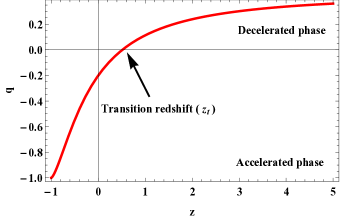
Figure 1: Plot of Deceleration parameter $\left(q\right)$ versus red-shift $\left(z\right)$.

Using Eqs. (28) and (29) in (18), we get the non-metricity scalar $Q$ as

$$Q=\frac{-18\left(1+2m\right)}{\left(m+2\right)^{2}}H^{2}.$$ (33)

We examine the Hubble’s horizon ( $L=H^{-1}$) as the IR cut-off of the system, where $H$ is the Hubble’s parameter of the model. Therefore, in symmetric teleparallel gravity the energy density of Barrow holographic dark energy (2) takes the form

$$\rho_{B}=CH^{2-\Delta}.$$ (34)

The motives for using this new formula introduced by Barrow is that he thinks it is important in comprehension the evolution of the Universe for a large horizon length $L$, in particular an anisotropic Universe.

From Eqs. (31) and (34) , we get the energy density of the Barrow holographic dark energy as

$$\rho_{B}=C\left[\frac{ne^{nt}}{\left(1+b\right)\left(e^{nt}-1\right)}\right]^{2-\Delta}.$$ (35)

Using (33) and (34) in (19), the energy density of the matter in terms of Hubble’s parameter as

$$\rho_{m}=\frac{-486\lambda\left(1+2m\right)^{2}}{\left(m+2\right)^{4}}H^{4}-CH^{2-\Delta}.$$ (36)

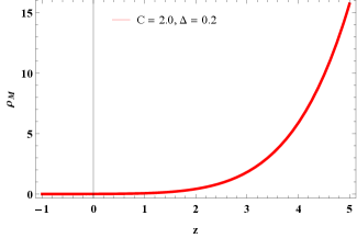
Figure 2: Plot of energy density $\left(\rho_{m}\right)$ of matter versus red-shift $\left(z\right)$.

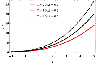
Figure 3: Plot of energy density $\left(\rho_{B}\right)$ of Barrow holographic dark energy versus red-shift $\left(z\right)$.

In Figs. 3 and 3, we plot the behavior of the energy density of matter $\left(\rho_{m}\right)$ and Barrow holographic dark energy $\left(\rho_{B}\right)$ with the Hubble’s horizon cut-off with respect to the red-shift $\left(z\right)$ for the appropriate values of model parameters, respectively. It is observed that both $\rho_{m}$ and $\rho_{B}$ are positive and decreasing function of red-shift while energy density of matter becomes null and energy density of Barrow holographic dark energy attends a specific small constant value.

The skewness parameter $\delta$ as

$$\delta=\frac{324\lambda\left(1+2m\right)\left(1-m\right)}{\rho_{B}\left(m+2\right)^{3}}H^{4}\left[\left(1+b\right)e^{-nt}-1\right].$$ (37)

Fig. 5 shows the evolution of the skewness parameter $\left(\delta\right)$ versus red-shift $z$. It can be observed that $\delta$ of our model varies between positive and negative values throughout cosmic evolution. Moreover, we can see that the skewness parameter at the initial epoch decreases until it reaches a negative value in the present epoch (i.e $z=0$) and in the future (i.e $z\rightarrow-1$). Therefore, our model is anisotropic throughout the evolution of the Universe. From Eqs. (35) and (38), we observe that the energy densities of matter and Barrow holographic dark energy are decreasing functions of cosmic time.

$$\rho_{m}=\frac{-486\lambda\left(1+2m\right)^{2}}{\left(m+2\right)^{4}}H^{4}-CH^{2-\Delta}.$$ (38)

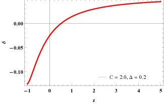
Figure 4: Plot of skewness parameter $\left(\delta\right)$ versus red-shift $\left(z\right)$

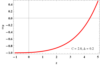
Figure 5: Plot of $\left(\omega_{B}\right)$ versus red-shift $\left(z\right)$.

The equation of state parameter of Barrow holographic dark energy is given by

$$\omega_{B}=\frac{-162\lambda\left(1+2m\right)}{C\left(m+2\right)^{3}}H^{2+\Delta}\left[\frac{\left(1+2m\right)}{\left(m+2\right)}+4\left\{\left(1+b\right)e^{-nt}-1\right\}\right].$$ (39)

The evolution of equation of state is shown as a function of red-shift $z$ in Fig. 5. From this figure, the equation of state parameter of our model transitions from positive to negative value with cosmic evolution, indicating the Universe’s initial phase of deceleration with positive pressure and the current phase of acceleration with negative pressure. Also, at $z=0$, $\omega_{B}$ approaches $-1$ in the current era.

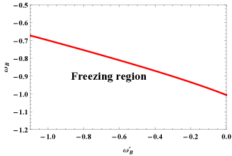
Figure 6: Plot of $\omega_{B}$ versus $\omega_{B}^{{}^{\prime}}$.

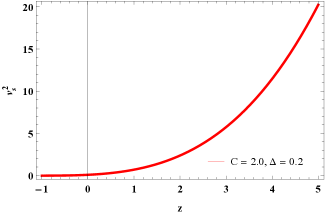
Figure 7: Plot of squared sound speed $\left(v_{s}^{2}\right)$ versus red-shift $\left(z\right)$.

We can see from Eq.(39), that the equation of state parameter is a function of time. However, the model starts from matter-dominated era, varies in the quintessence region $-1<\omega_{B}<-\frac{1}{3}$ and finally approached to phantom region $\omega_{B}<-1$. At present the current value of equation of state parameter is $\omega_{0}\sim-1$, i.e. the Universe is dominated by $\Lambda$ cold dark matter $\left(\Lambda CDM\right)$. The results obtained in our model are consistent with the constraints of the equation of state parameter for the Planks Collaboration and WMAP which give the ranges for Equation of state parameter as: $-0.92\leq\omega\leq-1.26$ (Planck+WP+Union 2.1), $-0.89\leq\omega\leq-1.38$ (Planck+WP+BAO), $-0.983\leq\omega\leq-1.162$ (WMAP+eCMB+BAO+H0). Finally, the behavior of the obtained model is in good agreement with recent observational data of SNe-Ia.

Next, the author Caldwell and Linder [50], proposed the ($\omega_{B}-\omega_{B}^{{}^{\prime}}$)- plane to describe the dynamical properties of the quintessence scalar field. In $\omega_{B}^{{}^{\prime}}$, prime designate the derivative of equation of state parameter with respect to $x=\ln a$. By ($\omega_{B}-\omega_{B}^{{}^{\prime}}$)- plane analysis, we consider two distinct thawing and freezing regions respectively corrosponds to $\left(\omega_{B}^{{}^{\prime}}>0\text{, }\omega_{B}<0\right)$ and $\left(\omega_{B}^{{}^{\prime}}<0\text{, }\omega_{B}<0\right)$.
Using Eq. (39), we get

$$\omega_{B}^{{}^{\prime}}=\frac{-162\lambda\left(1+2m\right)}{C\left(m+2\right)^{3}}H^{1+\Delta}\left[\left(2+\Delta\right)\frac{H}{\overset{.}{H}}\left\{\frac{\left(1+2m\right)}{\left(m+2\right)}+4\left\{\left(1+b\right)e^{-nt}-1\right\}\right\}-4n\left(1+b\right)e^{-nt}\right].$$ (40)

where $\overset{.}{H}=\frac{-n^{2}e^{nt}}{\left(e^{nt}-1\right)^{2}\left(b+1\right)}$ .
The plot of the ($\omega_{B}-\omega_{B}^{{}^{\prime}}$)- plane of the model is given in Fig. 7. Also, we can see that $\omega_{B}^{{}^{\prime}}<0$ and $\omega_{B}<0$ which indicates the freezing region of the Universe. In this scenario, the squared sound speed $\left(v_{s}^{2}\right)$ is used for studying the stability of the dark energy models which is given as $v_{s}^{2}=\frac{dp_{B}}{d\rho_{B}}=\frac{\overset{.}{p}_{B}}{\overset{.}{\rho}_{B}}$. If $v_{s}^{2}>0$, we obtain a stable model and if $v_{s}^{2}<0$, we obtain unstable model. For our Barrow holographic dark energy model, $v_{s}^{2}$ takes the following form

$$v_{s}^{2}=\frac{-648\lambda\left(1+2m\right)}{C\left(m+2\right)^{3}\left(2-\Delta\right)}H^{2+\Delta}\left[\frac{\left(1+2m\right)}{\left(m+2\right)}+\left(1+b\right)\left\{4-n\frac{H}{\overset{.}{H}}\right\}e^{-nt}-4\right]$$ (41)

Fig. 7 shows the evolution of the squared sound speed in terms of red-shift $(z)$. It is clear that the Barrow holographic dark energy model is stable i.e. $v_{s}^{2}>0$ with the cosmic expansion of the Universe.

Sahni et al. [51] have instituted the geometrical diagnostic pair named the state-finder pair $\left\{r,s\right\}$ to differentiate dark energy models. Here, $r$ is produced from the average scale factor $a$ and its derivatives with regard to the cosmic time up to the third-order and $s$ is a simple composite of $r$. The state-finder pair $\left\{r,s\right\}$ is defined as

$$r=\frac{\overset{...}{a}}{aH^{3}}\text{, \ \ }s=\frac{r-1}{3\left(q-\frac{1}{2}\right)}.$$ (42)

The values of the state-finder parameter for our model are observed as

$$r=1-\frac{3n+\left(1+b\right)^{2}\left(1-e^{-2nt}\right)}{\left(e^{nt}-1\right)}.$$ (43)

$$s=\frac{2\left(1+b\right)^{2}\left(1-e^{-2nt}\right)-6n}{\left(e^{nt}-1\right)\left[6\left(1+b\right)e^{-nt}-9\right]}.$$ (44)

For $\left\{r=1,s=0\right\}$, we obtain the $\Lambda CDM$ model, while for $\left\{r=1,s=1\right\}$, we obtain the cold dark matter $\left(CDM\right)$ limit. In addition, for $\left\{r<1,s>0\right\}$ we obtain a quintessence region. It can be observed from Fig. 8 that when $z\rightarrow-1$, $\left\{r=1,s=0\right\}$ and as $z=0$, $\left\{r<1,s>0\right\}$. This, indicates that our model starts from a quintessence epoch and approaches the $\Lambda CDM$ Universe.

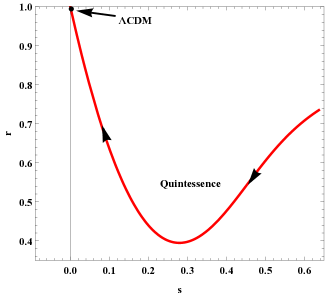
Figure 8: Plot of state-finder parameter $\left\{r,s\right\}$.

V Observational constraints

In this section, we have constrained the model parameters with the observational data. We have found the best fit value for the model parameters $b$, $n$ and $k$ and the current value of the Hubble’s parameter $H_{0}$ in our model. For this, we will use $51$ homogenized and model-independent Hubble’s parameter measurements in the range $0.07\leq z\leq 2.36$ [52]. In this set of $57$ Hubble’s data points, $31$ points measured via the method of Differential Age (DA) and remaining $26$ points through BAO and other methods (see Tabl. 1) [53]. The Hubble’s parameter $H$ in terms of red-shift $z$ as

$$H\left(z\right)=\frac{n}{\left(1+b\right)}\left[1+\left(k\left(1+z\right)\right)^{1+b}\right].$$ (45)

The technique $R^{2}$-test to find the best fit value of the model parameters defined by following statistical formula

$$R^{2}=1-\frac{\sum_{i=1}^{57}\left[\left(H_{i}\right)_{ob}-\left(H_{i}\right)_{th}\right]^{2}}{\sum_{i=1}^{57}\left[\left(H_{i}\right)_{ob}-\left(H_{i}\right)_{mean}\right]^{2}},$$ (46)

where, $\left(H_{i}\right)_{ob}$ and $\left(H_{i}\right)_{th}$ are observed and predicted values of Hubble’s parameter, respectively.

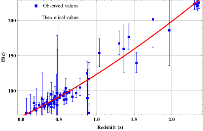
Figure 9: Best fit curve of Hubble’s parameter $\left(H\right)$ versus red-shift $\left(z\right)$.

By minimizing $R^{2}$, we find the best fit values for the model parameters $b=0.444$, $n=40.73$ and $k=1.159$ (with 95% confidence bounds). Also, we find $R^{2}=0.9335$ and root mean square error $\left(RMSE\right)=11.54$ for the model under consideration with $57$ Hubble’s parameter measurements. If $R^{2}=1$ corresponds to the ideal case when the observed data and corresponding values of theoretical function agree exactly. Now, Eq. (45) becomes

$$H\left(z\right)=28.2063+34.9047\left(1+z\right)^{1.444}.$$ (47)

Using Eq. (47), the current value of Hubble’s parameter $H$ for the obtained model, have calculated as $H_{0}=63.111\pm 11.54Km/s/Mpc$. Fig. 9 shows the best fit curve of the Hubble’s parameter versus red-shift $z$ using $57$ Hubble’s parameter measurements.

$z$	$H(z)$	$\sigma_{H}$	$z$	$H\left(z\right)$	$\sigma_{H}$
0.070	69	19.6	0.4783	80	99
0.90	69	12	0.480	97	62
0.120	68.6	26.2	0.593	104	13
0.170	83	8	0.6797	92	8
0.1791	75	4	0.7812	105	12
0.1993	75	5	0.8754	125	17
0.200	72.9	29.6	0.880	90	40
0.270	77	14	0.900	117	23
0.280	88.8	36.6	1.037	154	20
0.3519	83	14	1.300	168	17
0.3802	83	13.5	1.363	160	33.6
0.400	95	17	1.430	177	18
0.4004	77	10.2	1.530	140	14
0.4247	87.1	11.2	1.750	202	40
0.4497	92.8	12.9	1.965	186.5	50.4
0.470	89	34
$z$	$H\left(z\right)$	$\sigma_{H}$	$z$	$H\left(z\right)$	$\sigma_{H}$
0.24	79.69	2.99	0.52	94.35	2.64
0.30	81.7	6.22	0.56	93.34	2.3
0.31	78.18	4.74	0.57	87.6	7.8
0.34	83.8	3.66	0.57	96.8	3.4
0.35	82.7	9.1	0.59	98.48	3.18
0.36	79.94	3.38	0.60	87.9	6.1
0.38	81.5	1.9	0.61	97.3	2.1
0.40	82.04	2.03	0.64	98.82	2.98
0.43	86.45	3.97	0.73	97.3	7.0
0.44	82.6	7.8	2.30	224	8.6
0.44	84.81	1.83	2.33	224	8
0.48	87.90	2.03	2.34	222	8.5
0.51	90.4	1.9	2.36	226	9.3

Table 1: 57 points of $H(z)$ data: $31$ (DA) + $26$ (BAO+other) [53].

VI Conclusions

In this paper, we have considered a spatially homogeneous and anisotropic Bianchi type-I space-time in the presence of Barrow holographic dark energy (infrared cut-off is the Hubble’s horizon) suggested by Barrow recently (Physics Letters B 808 (2020): 135643) and matter in quadratic form of $f(Q)$ gravity i.e. $f(Q)=\lambda Q^{2}$ (where $\lambda<0$ is a constant). The exact solutions to the field equations are obtained assuming that the deceleration parameter $q$ is a function of the Hubble’s parameter $H$ i.e. $q=b-\frac{n}{H}$ (where $b$ and $n$ are constants). First, we have studied the behavior of this form of deceleration parameter given in Eq. (32) and it turns out that passes from positive to negative value as the red-shift increases and it converges towards $-1$ when $z=-1$. Hence, our model of the Universe goes from an early deceleration phase to a current acceleration phase which is in good agreement with recent observation data. Next, we have got the energy densities of matter and Barrow holographic dark energy both are positive decreases as Universe expands, the energy density of matter becomes null and energy density of Barrow holographic dark energy attends a specific small constant value. Also, the equation of state parameter of our model transitions from positive to negative value with cosmic evolution. The model starts from matter-dominated era, varies in the quintessence region $-1<\omega_{B}<-\frac{1}{3}$ and finally approached to $\Lambda$CDM region ($\omega_{B}=-1$). At present the current value of equation of state parameter is $\omega_{0}\sim-1$, i.e. the Universe is dominated by $\Lambda CDM$. Thus, the behavior of the obtained model is in good agreement with recent observational data.

The skewness parameter represents same behavior as that of the equation of state parameter. At the initial epoch it decreases until reaches a negative value in the present and future epoch which confirms that the model is anisotropic throughout the evolution of the Universe. For the proposed plane of Caldwell and Linder, it is observed that the equation of state parameter and the argument of equation of state parameter with lna both are non-negative which represents freezing region of the Universe where as the stability parameter in term of squared sound speed is stable i.e. $v_{s}^{2}>0$ with the cosmic expansion of the Universe. In $\left\{r,s\right\}$-plane, Initially $\left\{r<1,s>0\right\}$ and with cosmic expansion $\left\{r,s\right\}=\left\{1,0\right\}$. This, indicates that our model starts from a quintessence epoch and approaches the $\Lambda CDM$ Universe.

- [1] A. G. Riess et al., Astron. J. 116, 1009 (1998).
- [2] S. Perlmutter et al., Nature 391, 51 (1998).
- [3] Planck Collab. (P.A.R. Ade et al.), Astron. Astrophys. 594, A13 (2016).
- [4] Planck Collab. (N. Aghanim et al.), Astron. Astrophys. 641, A6 (2020).
- [5] A. G. Cohen, D. B. Kaplan and A. E. Nelson, Phys. Rev. Lett. 82, 4971 (1999).
- [6] B. Wang et al., Rep. Prog. Phys. 79, 096901 (2016).
- [7] Y. Wang and M. Li, Phys. Rep. 1, 696 (2017).
- [8] S. Srivastava, U. K. Sharma and A. Pradhan, New Astron. 68, 57 (2019).
- [9] S. H. Shekh, Phys. Dark Universe 33, 100850 (2021).
- [10] S. H. Shekh, P. H. R. S. Moraes and P. K. Sahoo, Universe 7, 67 (2021).
- [11] M. Koussour and M. Bennai, Int J Mod Phys A 37, 05 (2022).
- [12] S. H. Shekh, V. R. Chirde and P. K. Sahoo, Commun. Theor. Phys. 72, 085402 (2020).
- [13] A. Pradhan, A. Dixit and V. K. Bhardwaj, Int. J. of Mod. Phy. A 36, 2150030 (2021) arXiv:2101.00176 [gr-qc]
- [14] V. K. Bhardwaj, A. Dixit, A. Pradhan, S. Krishannair, arXiv:2109.12963v2 [gr-qc]
- [15] J. D. Barrow, Phys. Lett. B 808, 135643 (2020).
- [16] S. Wang, Y. Wang and M. Li, Phys. Rept. 696, 1 (2017).
- [17] P. K. Nandhida, T. K. Mathew, arXiv:2112.07310 [gr-qc].
- [18] L. N. Granda and A. Oliveros, Phys. Lett. B 669, 5 (2008).
- [19] P. Adhikary, S. Das, S. Basilakos, and E. N. Saridakis, Phys. Rev. D 104, 123519 (2021).
- [20] A. Sarkar and S. Chattopadhyay, Int. J. of Geom. Meth. in Modern Physics 18, 09 (2021).
- [21] Nojiri, Shin’ichi, and Sergei D. Odintsov, Phys. Rept. 505, 2-4 (2011).
- [22] Nojiri, Shin’ichi, and Sergei D. Odintsov, Gen. Relativ. Gravit. 36, 8 (2004).
- [23] Nojiri, Shin’ichi, and Sergei D. Odintsov, Phys. Lett. B 657, 4-5 (2007).
- [24] G. Bengochea and R. Ferraro, Phys. Rev. D 79, 124019 (2009).
- [25] K. Bamba et al., J. Cosmol. Astropart. Phys. 01 021 (2011).
- [26] Bahamonde, Sebastian, et al., arXiv preprint arXiv:2106.13793 (2021).
- [27] T. Harko, F. S. N. Lobo, S. Nojiri and S. D. Odintsov, Phys. Rev. D 84, 024020 (2011).
- [28] P. K. Sahoo, B. Mishra and R. Chakradhar, Eur. Phys. J. Plus. 129, 49 (2014).
- [29] M. Koussour and M. Bennai, Int. J. of Geom. Meth. in Modern Physics 19, 03 (2021).
- [30] M. Koussour and M. Bennai, Afrika Matematika 33, 01 (2022).
- [31] S. Nojiri and S. D. Odintsov, J. Phys. Conf. Ser. 66, 012005 (2007).
- [32] M. Koussour et al., Nucl. Phys. B 978, 115738 (2022).
- [33] S. H. Shekh, S.D. Katore, V.R. Chirde and S.V. Raut, New Astron. 84, 101535 (2021).
- [34] S. H. Shekh, S. Arora, V. R. Chirde and P. K. Sahoo, Int. J. of Geo. Methods in Mod. Phy. 17, 2050048 (2020).
- [35] S. H. Shekh, New Astron. 83, 101464 (2021)..
- [36] S. H. Shekh, V. R. Chirde and P. K. Sahoo, Commun. Theor. Phys. 72, 085402 (2020).
- [37] J. B. Jimenez et al., Phys. Rev. D, 98 044048 (2018).
- [38] J.B. Jimenez et al., Phys. Rev. D 101, 103507 (2020).
- [39] W. Khyllep et al., Phys. Rev. D 103, 103521 (2021).
- [40] S. Mandal et al., Phys. Rev. D 102, 124029 (2020).
- [41] S. Mandal et al., Phys. Rev. D 102, 024057 (2020).
- [42] N. Dimakis, A. Paliathanasis and T. Christodoulakis, Class. Quant. Grav. 38, 225003 (2021). arXiv:2108.01970 [gr-qc].
- [43] W. Khyllep, A. Paliathanasis and J. Dutta, Phys. Rev. D 103, 103521 (2021).
- [44] T. Harko et al., Phys. Rev. D 98, 084043 (2018).
- [45] N. Frusciante, Phys. Rev. D 103, 4 (2021).
- [46] Tiwari, R. K., Değer Sofuoğlu and V. K. Dubey, Int. J. of Geo. Methods in Mod. Phy. 17, 12 (2020).
- [47] P. Sahoo et al., Communications in Theoretical Physics (2022). doi: 10.1088/1572-9494/ac8d8a.
- [48] S. Capozziello and R. D’Agostino, Phys. Lett. B 832, 137229 (2022).
- [49] A. De et al., Eur. Phys. J. C 82 1-11 (2022).
- [50] R.R. Caldwell and E.V. Linder, Phys. Rev. Lett. 95, 141301 (2005).
- [51] V. Sahni et al., JETP Lett. 77, 201 (2003).
- [52] G. S. Sharov and V. O. Vasiliev, Mathematical Modelling and Geometry 6, 1 (2018).
- [53] C. H. Chuang and Y. Wang, Mon. Not. Roy. Astron. Soc. 435, 255 (2013).