Kerr-Sen-like Lorentz violating black holes and Superradiance phenomena

Abstract

Abstract

A Kerr-Sen-like black hole solution results from Einstein-bumblebee gravity. It contains a Lorentz violating (LV) parameter that enters when the bumblebee field receives vacuum expectation value through a spontaneously breaking of the symmetry of the classical action. The geometrical structure concerning the singularity of this spacetime is studied with reference to the parameters involved in the Kerr-Sen-like metric. We introduce this Einstein-bumblebee modified gravity to probe the role of spontaneous Lorentz violation on the superradiance scattering phenomena and the instability associated with it. We observe that for the low-frequency range of the scalar wave the superradiance scattering gets enhanced when the Lorentz-violating parameter $\ell$ takes the negative values and it reduces when values of $\ell$ are positive. The study of the black hole bomb issue reveals that for the negative values of $\ell$, the parameter space of the scalar field instability increase prominently, however, for its positive values, it shows a considerable reduction. We also tried to put constraints on the parameters contained in the Kerr-Sen-like black hole by comparing the deformation of the shadow produced by the black hole parameters with the observed deviation from circularity and the angular deviation from the $M87*$ data.

I Introduction

In a gravitational system, the scattering of radiation off absorbing rotating objects produce waves with amplitude larger than incident one under certain conditions which is known as rotational superradiance ZEL0 ; ZEL1 . In 1971, Zel’dovich showed that scattering of radiation off rotating absorbing surfaces result in waves with a larger amplitude as $\omega<m\Omega$ where $\omega$ is the frequency of the incident monochromatic radiation with m, the azimuthal number with respect to the rotation axis and $\Omega$ is the angular velocity of the rotating gravitational system. For review we would like to mention the lecture notes REVIEW , and the references therein. Rotational superradiance belongs to a wider class of classical problems displaying stimulated or spontaneous energy emission, such as the Vavilov-Cherenkov effect, the anomalous Doppler effect. When quantum effects were incorporated, it was argued that rotational superradiance would become a spontaneous process and that rotating bodies including black holes would slow down by spontaneous emission of photons. From the historic perspective, the discovery of black-hole evaporation HAW was well understood from the studies of black-hole superradiance.

Interest in the study of black-hole superradiance has recently been revived in different areas, including astrophysics, high-energy physics via the gauge/gravity duality along with fundamental issues in General Relativity. Superradiant instabilities can be used to constrain the mass of ultralight degrees of freedom INST00 ; INST0 ; INST1 ; INST2 , with important applications to dark-matter searches. The black hole superradiance is also associated with the existence of new asymptotically flat hairy black-hole solutions HAIR and with phase transitions between spinning or charged black objects and asymptotically anti-de Sitter (AdS) spacetime ADS0 ; ADS1 ; ADS2 or in higher dimensions MSHO . Finally, the knowledge of superradiance is instrumental in describing the stability of black holes and in determining the fate of the gravitational collapse in confining geometries ADS1 .

During the last few decades, the standard theories of general relativity have been continuing to explain many important experimental results. However, there is still some room to the use of alternative theories of the general theory of relativity. From a theoretical viewpoint, having an ultraviolet complete theory of general relativity is complimentary as well as supportive. Moreover from the observational point of view, general relativity has shortcomings to describe some gravitational phenomena at a large scale such as the dark side of the universe. These shortcomings automatically demand modified theories of general relativity. The modifications may render some imprints in astrophysical phenomena where it is expected that the strong gravity triggers the events in the vicinity of celestial bodies like astrophysical black holes and neutron stars. Black holes can be used as a potential probe to investigate the possible high-energy modifications to general relativity in the regime where gravity is sufficiently strong. In this respect, the use of alternative theories of gravity would be of cardinal importance to study the astrophysical aspects of black hole. The important astrophysical phenomena namely black hole superradiance is extremely sensitive to the spacetime geometries linked with it. Recently, several investigations have been carried out on superradiance phenomena and on the issues closely linked to it with the extended framework of modified theories of gravity MODG0 ; MODG1 ; MODG2 ; MODG3 ; MODG4 ; MODG5 ; MODG6 ; MODG7 ; MODG8 ; MODG9 ; MODG10 ; MODG11 ; MODG12 ; MODG13 . As an extension in this direction, an attempt has been made here to study the superradiance of the spinning black holes within the framework of Lorentz-violating gravity. It is commonly known as the ’Einstein-bumblebee model KOSTEL0 which involves the innovative ’spontaneous Lorentz symmetry breaking’ principle. From the theoretical point of view, it arrived from one of the standard issues of quantization of gravity through string theory. Although the Lorentz symmetry is the fundamental underlying symmetry of two successful field theories describing the universe, i.e. GR and the standard model of particle, however, it is more or less accepted from all corners that it may break at quantum gravity scales. The LSB has been introduced through the formulation of an effective field theory, known as ’standard model extension(SME), where particle standard model along with GR has been attempted to bring together in one framework, and every operator is expected to break the Lorentz symmetry KOSTEL1 ; COLL0 ; COLL1 ; COLE . Standard model extension provides essential inputs to probe LSB both in high energy particle physics and astrophysics. The SME can be used in analysis of most modern experimental results indeed. Einstein- bumblebee model is essentially a simple model that contains Lorentz symmetry breaking scenario in a significant manner in which the physical Lorentz symmetry breaks down through an axial vector field known as the bumblebee field. The breaking of the Lorentz symmetry in a local Lorentz frame takes place when at least one quantity carrying local Lorentz indices receives a non-vanishing vacuum expectation value. In the Einstein bumblebee model, it is the bumblebee field that receives it. Over the last few years, a remarkable enthusiasm has been noticed among the physicist to study the different interesting physical phenomena in the framework of Einstein Bumblebee model SEIF ; JPAR ; DCAP ; CASANA ; OLIV ; OAV ; OAV1 ; OLIVE ; DING . Recently, the superradiance phenomenon corresponding to Kerr black hole is studied in MK in this framework. The black hole solution considered there was Kerr-like. The study of superradiance phenomena of black holes through the Einstein bumblebee model using Kerr-sen-like black hole solution is a natural extension. This new investigation is likely to be useful in the study of black holes in the quantum gravity realm since it would be possible to compare the contribution of LV to the superradiance phenomenon.

The article is organized as follows. In Sec.2 a brief discussion of Einstein-bumblebee gravity with Kerr-Sen-like black hole solutionis given. A subsection of Sec.2 contains the discussion of Horizon, Ergosphere, and static limit surface. Sec.3 is devoted with the superradience scattering of scalar field off Kerr-Sen-like black hole. Amplification factor for superradiance sacttering off Kerr-Sen-like black hole has been calculated in Sec.4 and a subsection of which is devoted with the superradiant instability issue for Kerr-Sen-like black hole. In Sec.5 Constraining of the parameter of this black hole is made from the observed data for $\mathrm{M}87^{*}$. Final Sec. 6 contains a brief summary and discussions.

II EXACT KERR-SEN LIKE BLACK HOLE SOLUTION IN EINSTEIN-BUMBLEBEE MODEL

Einstein-bumblebee theory is an extension of Einstein’s theory where a vector boson is involved that plays a pivotal role in the existing symmetry of Einstein’s theory CASANA ; ARS ; ARS1 ; OLIVE ; DING ; ARS2 . It is an effective classical field theory where the vector field involved in the theory receives vacuum expectation when spontaneous braking of an existing symmetry of the action takes place and a Lorentz violation enters into the theory as an outcome. Einstein-bumblebee theory is described by the action

$$\mathcal{S}=\int d^{4}x\sqrt{-g}\left[\frac{1}{16\pi G_{N}}\left(\mathcal{R}+\varrho B^{\mu}B^{\nu}\mathcal{R}_{\mu\nu}\right)-\frac{1}{4}B^{\mu\nu}B_{\mu\nu}-V\left(B^{\mu}\right)\right].$$ (1)

Here $\varrho^{2}$ stands for the real coupling constant. It controls the non-minimal gravity interaction to the bumblebee field $B_{\mu}$ (with the mass dimension 1). The coupling constant $\varrho^{2}$ has mass dimension $-1$.

The action (1) leads to the following gravitational field equation in vacuum

$$\mathcal{R}_{\mu\nu}-\frac{1}{2}g_{\mu\nu}\mathcal{R}=\kappa T_{\mu\nu}^{B},$$ (2)

where $\kappa=8\pi G_{N}$ is the gravitational coupling. The bumblebee energy momentum tensor $T_{\mu\nu}^{B}$ reads

$$T_{\mu\nu}^{B} = B_{\mu\alpha}B_{\nu}^{\alpha}-\frac{1}{4}g_{\mu\nu}B^{\alpha\beta}B_{\alpha\beta}-g_{\mu\nu}V+2B_{\mu}B_{\nu}V^{\prime}$$ (3)

$$+ \frac{\varrho}{\kappa}[\frac{1}{2}g_{\mu\nu}B^{\alpha}B^{\beta}R_{\alpha\beta}-B_{\mu}B^{\alpha}R_{\alpha\nu}-B_{\nu}B^{\alpha}R_{\alpha\mu}$$

$$+ \frac{1}{2}\nabla_{\alpha}\nabla_{\mu}\left(B^{\alpha}B_{\nu}\right)+\frac{1}{2}\nabla_{\alpha}\nabla_{\nu}\left(B^{\alpha}B_{\mu}\right)-\frac{1}{2}\nabla^{2}\left(B^{\mu}B_{\nu}\right)-\frac{1}{2}g_{\mu\nu}\nabla_{\alpha}\nabla_{\beta}\left(B^{\alpha}B^{\beta}\right)].$$

Here prime(’) denotes the differentiation with respect to the argument.

Einstein’s equation in the present situation is generalized to

$$\mathcal{R}_{\mu\nu}-\kappa b_{\mu\alpha}b_{\nu}^{\alpha}+\frac{\kappa}{4}g_{\mu\nu}b^{\alpha\beta}b_{\alpha\beta}+\varrho b_{\mu}b^{\alpha}\mathcal{R}_{\alpha\nu}+\varrho b_{\nu}b^{\alpha}\mathcal{R}_{\alpha\mu}$$

$$-\frac{\varrho}{2}g_{\mu\nu}b^{\alpha}b^{\beta}\mathcal{R}_{\alpha\beta}-\frac{\varrho}{2}\left[\nabla_{\alpha}\nabla_{\mu}\left(b^{\alpha}b_{\nu}\right)+\nabla_{\alpha}\nabla_{\nu}\left(b^{\alpha}b_{\mu}\right)-\nabla^{2}\left(b_{\mu}b_{\nu}\right)\right]=0$$

$$\Rightarrow\bar{R}_{\mu\nu}=0,$$ (4)

with

$$\bar{R}_{\mu\nu} = \mathcal{R}_{\mu\nu}-\kappa b_{\mu\alpha}b_{\nu}^{\alpha}+\frac{\kappa}{4}g_{\mu\nu}b^{\alpha\beta}b_{\alpha\beta}+\varrho b_{\mu}b^{\alpha}\mathcal{R}_{\alpha\nu}+\varrho b_{\nu}b^{\alpha}\mathcal{R}_{\alpha\mu}-\frac{\varrho}{2}g_{\mu\nu}b^{\alpha}b^{\beta}\mathcal{R}_{\alpha\beta}+\bar{B}_{\mu\nu},$$

$$\bar{B}_{\mu\nu} = -\frac{\varrho}{2}\left[\nabla_{\alpha}\nabla_{\mu}\left(b^{\alpha}b_{\nu}\right)+\nabla_{\alpha}\nabla_{\nu}\left(b^{\alpha}b_{\mu}\right)-\nabla^{2}\left(b_{\mu}b_{\nu}\right)\right].$$ (5)

If we now adopt the standard Boyer-Lindquist coordinates we find that the underlying generalized gravity model admits a Kerr-Sen-like black hole solution:

$$ds^{2}=-\left(1-\frac{2Mr}{\rho^{2}}\right)dt^{2}-\frac{4Mra\sqrt{1+\ell}\sin^{2}\theta}{\rho^{2}}dtd\varphi+\frac{\rho^{2}}{\Delta}dr^{2}+\rho^{2}d\theta^{2}+\frac{A\sin^{2}\theta}{\rho^{2}}d\varphi^{2},$$ (6)

where

$$\rho^{2}=r(r+b)+(1+\ell)a^{2}\cos^{2}\theta,\Delta=\frac{r(r+b)-2Mr}{1+\ell}+a^{2},A=\left[r(r+b)+(1+\ell)a^{2}\right]^{2}-\Delta(1+\ell)^{2}a^{2}\sin^{2}\theta.$$ (7)

Here $a=\frac{J}{M}$ represents the rotation (Kerr) parameter $b=\frac{Q^{2}}{M}$, the Sen parameter related to the electric charge, and $\ell$ the Lorentz-violating parameter. M, J, and Q are representing respectively the mass, angular momentum, and charge of the black hole. Note that when $\ell\rightarrow 0$ it recovers the usual Kerr-Sen metric ASEN .

II.1 Horizon, Ergosphere, and static limit surface

The metric is singular when $\Delta=0$. The roots of the equation depend on the parameter $M$,$a$, $b$, and $\ell$. Having a maximum of two real roots, or two equal roots, and no real roots are the possibilities to occur from the condition$\Delta=0$ SGG ; SGG1 ; SGG2 ; TJDP . The horizons correspond to the two real roots which are given by

$$r_{\pm}=M-\frac{b}{2}\pm\frac{\sqrt{(b-2M)^{2}-4a^{2}(1+\ell)}}{2},$$ (8)

where $\pm$ signs correspond to the outer and inner horizon respectively. The event horizon and Cauchy horizon are labelled with $r_{eh}$ and $r_{ch}$ respectively. We will have a black hole only when

$$|b-2M|\geq 2a\sqrt{1+l}.$$ (9)

When $r_{-}=r_{+}$ we have extremal black hole. The parameter space $(a,b)$ for three different values values of Lorentz violating parameter $\ell=-0.5,0$, and $+0.5$ are shown here.

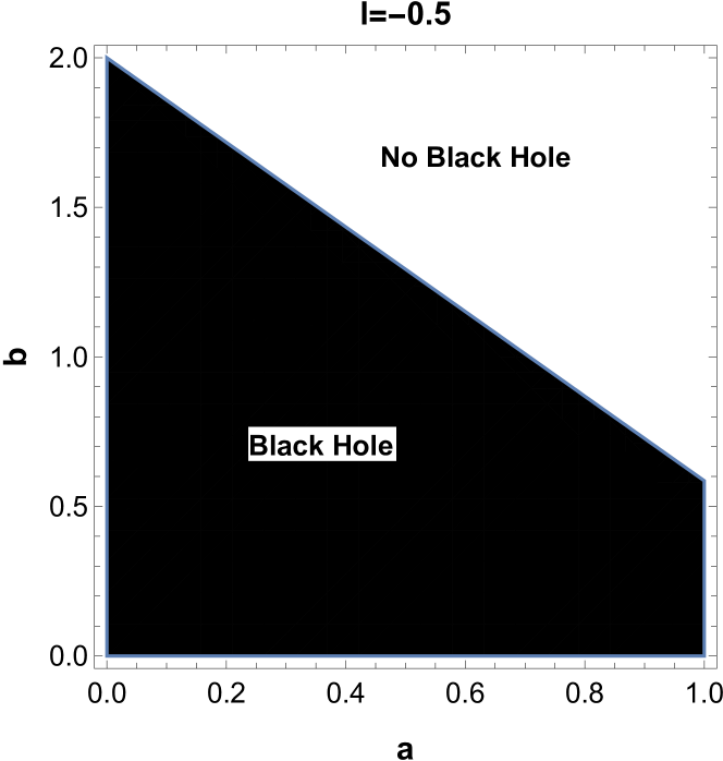
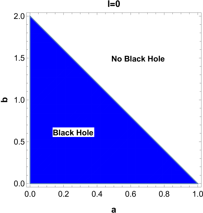
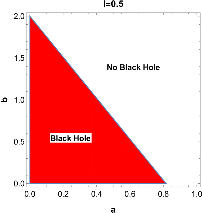
Figure 1: Parameter space($a$,$b$) for various values of $l$.

Fig.1 shows that parameter space for which we have a black hole is shrinking with an increase in the LV parameter $\ell$. So increase in $\ell$ makes the system less probable for having a black hole and the reverse is the case when LV parameter $\ell$ decreases. We now plot the $\Delta$ versus $r/M$ for various different variation of $a$, $b$, and $\ell$. In the plots when the variation of one parameter is considered the other two are held fixed.

From Fig. 2 and Fig. 3, we readily observe that there exist a critical value $a_{c}$ for the parameter $a$ for fixed values of $bl$ and $l$. Similarly, there is a critical value $b_{c}$ for the parameter $b$ when the parameter $a$ and $l$ care kept fixed. For fixed values of the parameter $b$ and $a$, $l_{c}$ comes out as critical value for the parameter $\ell$. At these critical values two roots of the $\Delta=0$ becomes identical which indicate extremal black holes. For instance, when $b=0.7,l=0.4$ we have $a_{c}=0.54935$, when $a=0.6,l=0.4$ we have $b_{c}=0.580141$, and when $a=0.6,b=0.7$ we have $l_{c}=0.173611$. Therefore, for $a<a_{c}$ we have black hole and for $a>a_{c}$ we have naked singularity. Similarly, $b<b_{c}$ indicates existence of a black hole and for $b>b_{c}$ it is a naked singularity. For $l<l_{c}$, in a similar way, we have black hole and $l>l_{c}$ signifies naked singularity.

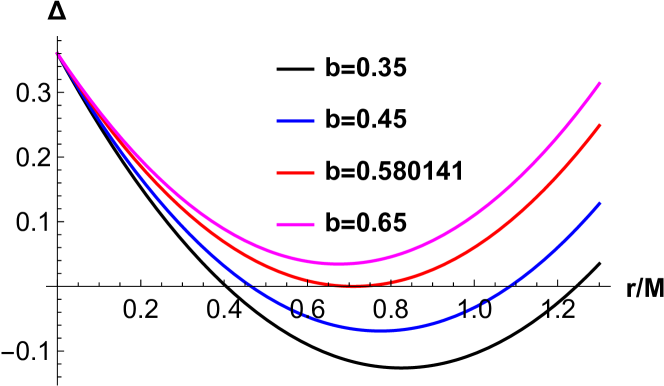
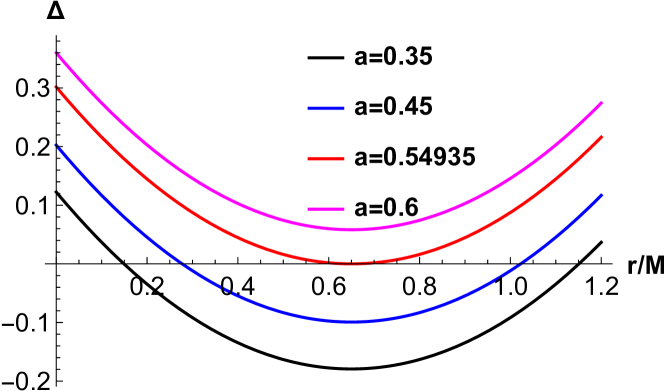
Figure 2: The left one gives variation of $\Delta$ for various values of $b$ with $a=0.6$ and $l=0.4$ and the right one gives variation for various values of $a$ with $b=0.7$ and $l=0.4$.

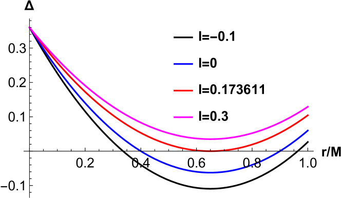
Figure 3: It gives variation of $\Delta$for various values of $l$ with $b=0.7$ and $a=0.6$.

Let us now turn towards the static limit surface (SLS) where the asymptotic time-translational Killing vector becomes null which gives

$$g_{tt}=\rho^{2}-2Mr=0.$$ (10)

The real positive solutions of the above equation give radial coordinates of the ergosphere given by

$$r_{\pm}^{ergo}=M-\frac{b}{2}\pm\frac{\sqrt{(b-2M)^{2}-4a^{2}(1+\ell)\cos^{2}\theta}}{2}.$$ (11)

Inside the SLS no observer can stay static and they are bound to co-rotate around the black hole. The region between the SLS and the event horizon is called the ergosphere shown below in Fig. 4. According to Penrose PENR ; PENR1 energy can be extracted from black hole’s ergosphere.

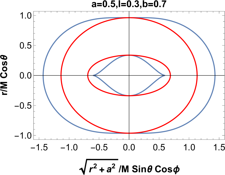
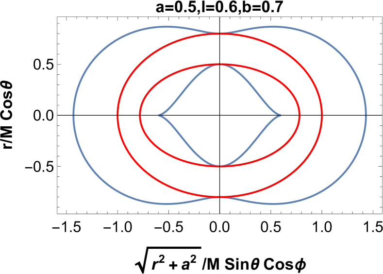
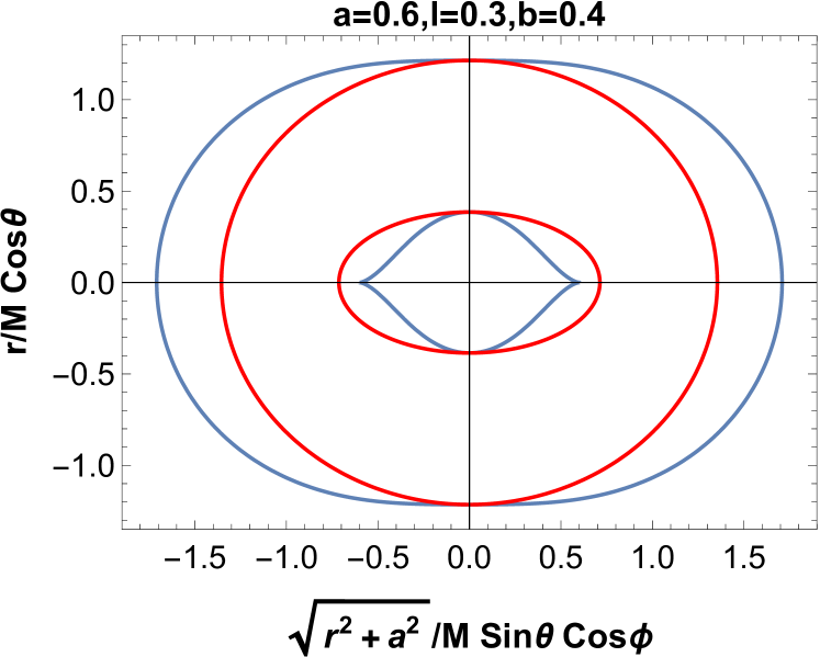
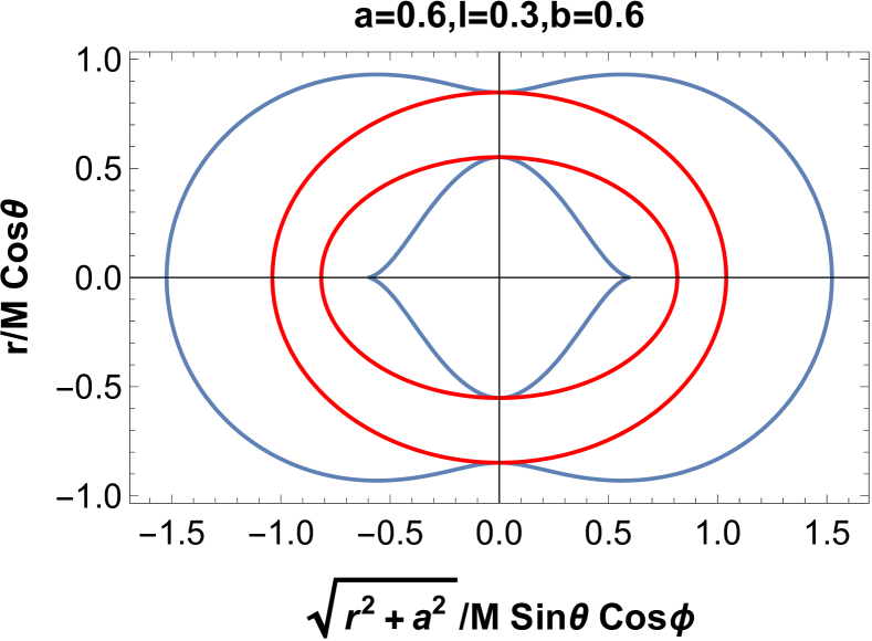
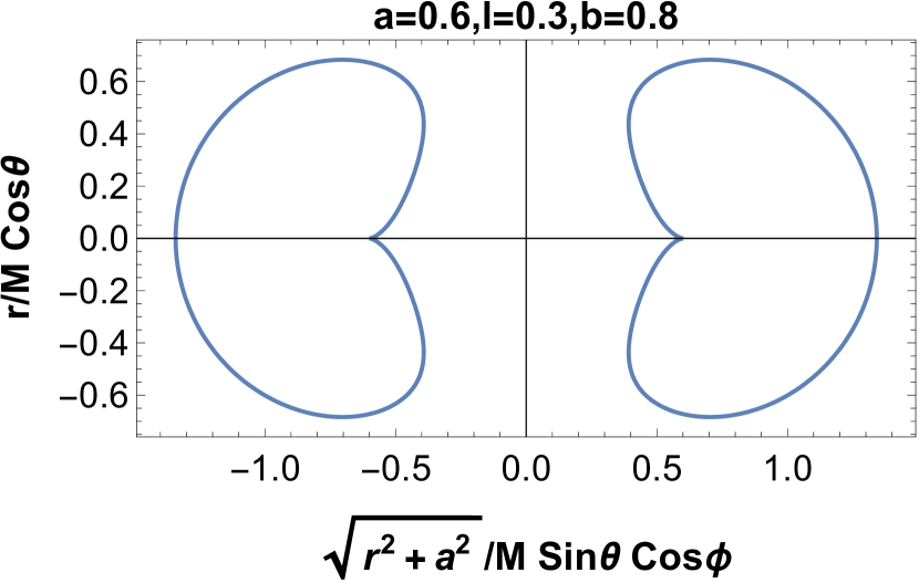
Figure 4: The cross-section of event horizon (outer red line), SLS (outer blue dotted line) and ergoregion of Kerr-Sen like black holes.

Fig. 4 shows that the shape of the ergosphere closely depends on parameters $a,b,$ and $l$. A careful look reveals that the size of the ergosphere is enhancing with the increase in the LV parameter $\ell$ when $a$ and $b$ remain fixed. The value of the parameter $b$ also has an influence on the size of the ergosphere. The size of the ergosphere increases with the increase in the value of the parameter $b$ as well when $a$ and $l$ remain unchanged.

Horizon angular velocity is found out to be

$$\hat{\Omega}=\frac{a\sqrt{1+l}}{r_{eh}\left(r_{eh}+b\right)+a^{2}\left(1+\ell\right)}.$$ (12)

III Superradience scattering of scalar field off Kerr-Sen-like black hole

To study the superradiance scattering of a scalar field $\Phi$ with mass $\mu$ we consider the Klein-Gordon equation in curved spacetime

$$\left(\bigtriangledown_{\alpha}\bigtriangledown^{\alpha}+\mu^{2}\right)\Phi(t,r,\theta,\phi)=\left[\frac{-1}{\sqrt{-g}}\partial_{\sigma}\left(g^{\sigma\tau}\sqrt{-g}\partial_{\tau}\right)+\mu^{2}\right]\Phi(t,r,\theta,\phi) = 0.$$ (13)

Adopting the separation of variables method on the equation (13) it is possible to separate it into radial and angular part using the following ansatz in the standard Boyer-Lindquist coordinates $(t,r,\theta,\phi)$

$$\Phi(t,r,\theta,\phi)=R_{\omega jm}(r)\Theta(\theta)e^{-i\omega t}e^{im\phi},\quad j\geq 0,\quad-j\leq m\leq j,\quad\omega>0,$$ (14)

where $R_{\omega jm}(r)$ is the radial function and $\Theta(\theta)$ is the oblate spheroidal wave function. The symbols $j$, $m$, and $\omega$ respectively stand for the angular eigenfunction, angular quantum number, and the positive frequency of the field, which is under investigation, as measured by a far away observer. Using the the ansatz (14) the differential equation (13), is found to get separated into the following two ordinary differential equations. For radial part the equation reads

$$\frac{d}{dr}(\Delta\frac{dR_{\omega jm}(r)}{dr})+(\frac{((r(r+b)+a^{2}(1+\ell))\omega-am\sqrt{1+\ell})^{2}}{\Delta(1+\ell)})R_{\omega lm}(r)$$

$$-(\mu^{2}r(r+b)+j(j+1)+a^{2}(1+\ell)\omega^{2}-2m\omega a\sqrt{1+\ell})R_{\omega lm}(r)=0,$$ (15)

and for the angular part it reads

$$\sin\theta\frac{d}{d\theta}\left(\sin\theta\frac{d\Theta_{\omega jm}(\theta)}{d\theta}\right)+\left(j(j+1)\sin^{2}\theta-\left(\left(a\sqrt{1+\ell}\omega\sin^{2}\theta-m\right)^{2}\right)\right)\Theta_{\omega jm}(\theta)$$

$$+a^{2}(1+\ell)\mu^{2}\sin^{2}\theta\cos^{2}\theta~{}\Theta_{\omega jm}(\theta)=0.$$ (16)

We can have a general solution of the radial equation (15) using the earlier investigation BEZERRA ; KRANIOTIS . We have given it as an appendix-A. However we are intended to study the scattering of the field $\Phi$ following the articles STRO1 ; STRO2 ; TEUK ; PAGE , and in this situation we have used the asymptotic matching procedure which is explicitely used in RAN . This article however is an extension of the important works STRO1 ; STRO2 ; TEUK ; PAGE . Use of asymptotic matching also has been found in MK . This led us to land onto the required result without using the general solution. Let us first focus on the radial equation. To deal with the radial equation according to our need we apply a Regge-Wheeler-like coordinate $r_{*}$ which is defined by

$$r_{*}\equiv\int dr\frac{r(r+b)+a^{2}(1+\ell)}{\Delta},\quad\left(r_{*}\rightarrow-\infty\quad\text{at event horizon},\quad r_{*}\rightarrow\infty\quad\text{at infinity}\right)$$ (17)

To transform the equation into the desired shape, we introduce a new radial function $\mathcal{R}_{\omega jm}\left(r_{*}\right)=\sqrt{r(r+b)+a^{2}(1+\ell)}R_{\omega jm}(r)$. After a few steps of algebra, we obtain the radial equation with our desired form where an effective potential took its entry into the picture.

$$\frac{d^{2}\mathcal{R}_{\omega lm}\left(r_{*}\right)}{dr_{*}^{2}}+V_{\omega jm}(r)\mathcal{R}_{\omega jm}\left(r_{*}\right)=0.$$ (18)

The effective potential that has the crucial role on the scattering reads

$$V_{\omega jm}(r) = \frac{1}{1+\ell}\left(\omega-\frac{m\hat{a}}{r(r+b)+\hat{a}^{2}}\right)^{2}-\frac{\Delta}{\left(r(r+b)+\hat{a}^{2}\right)^{2}}\left[\right.j(j+1)+\hat{a}^{2}\omega^{2}-2m\hat{a}\omega+\mu^{2}r(r+b)$$

$$\left.+\sqrt{r(r+b)+\hat{a}^{2}}\frac{d}{dr}\left(\frac{\Delta(2r+b)}{2\left(r(r+b)+\hat{a}^{2}\right)^{\frac{3}{2}}}\right)\right],$$

where $\tilde{a}=a(1+\ell)^{\frac{1}{2}}$. We are intended to study the scattering of the scalar field $\Phi$ under this effective potential. In this context, it is beneficial to study the asymptotic behavior of the scattering potential at the event horizon and at spatial infinity. In the asymptotic limit the potential at the event horizon looks

$$\lim_{r\rightarrow r_{eh}}V_{\omega jm}(r)=\frac{1}{1+\ell}\left(\omega-m\tilde{\Omega}_{h}\right)^{2}\equiv k_{eh}^{2},$$ (20)

$$\lim_{r\rightarrow\infty}V_{\omega jm}(r)=\omega^{2}-\lim_{r\rightarrow\infty}\frac{\mu^{2}r(r+b)\Delta}{\left(r(r+b)+\tilde{a}^{2}\right)^{2}}=\frac{\omega^{2}}{1+\ell}-\hat{\mu}^{2}\equiv k_{\infty}^{2},~{}~{}~{}\hat{\mu}=\frac{\mu}{\sqrt{\ell+1}}.$$ (21)

Note that at the two extremal points, event horizon and spatial infinity, the potential asymptotically shows constant behavior. However, the values of the constants are different indeed.

We are now in a position to see the asymptotic behavior of the radial equation. It is found that the radial equation (18) has the following asymptotic solutions

$$R_{\omega jm}(r)\rightarrow\left\{\begin{array}[]{cl}\frac{A_{in}^{eh}e^{-ik_{eh}r_{*}}}{\sqrt{r_{eh}(r_{eh}+b)+\hat{a}^{2}}}&\text{ for }r\rightarrow r_{eh}\\ \mathcal{A}_{in}^{\infty}\frac{e^{-ik_{\infty}r_{*}}}{r}+\mathcal{A}_{ref}^{\infty}\frac{e^{ik_{\infty}r_{*}}}{r}&\text{ for }r\rightarrow\infty\end{array}\right.$$ (22)

Here $\mathcal{A}_{in}^{eh}$ represents the amplitude of the incoming scalar wave at event horizon(”eh”), and $\mathcal{A}_{in}^{\infty}$ is the corresponding quantity of the incoming scalar wave at infinity$("\infty")$. Along with these, the amplitude of the reflected part of scalar wave at infinity $("\infty")$ is $\mathcal{A}_{ref}^{\infty}$.

Let us now compute the Wronskian for the region adjacent to the event horizon and at infinity. It is found that Wronskian for this region is

$$W_{eh}=\left(R_{\omega jm}^{eh}\frac{dR_{\omega jm}^{*eh}}{dr_{*}}-R_{\omega jm}^{*eh}\frac{dR_{\omega jm}^{eh}}{dr_{*}}\right),$$ (23)

and the Wronskian at infinity reads

$$W_{\infty}=\left(R_{\omega jm}^{\infty}\frac{dR_{\omega jm}^{*\infty}}{dr_{*}}-R_{\omega jm}^{*\infty}\frac{dR_{\omega jm}^{\infty}}{dr_{*}}\right).$$ (24)

The solutions are linearly independent. From the knowledge of standard theory of ordinary differential equation it can be understandable that the Wronskian corresponding to the solutions will be independent of $r^{*}$. Thus, the Wronskian evaluated at horizon does amenable to equate with the Wronskian evaluated at infinity. In physical sense, it is reflecting the flux conservation REVIEW . It results an important relation between the amplitudes of incoming and reflected waves at different regions of interest.

$$\left|\mathcal{A}_{ref}^{\infty}\right|^{2}=\left|\mathcal{A}_{in}^{\infty}\right|^{2}-\frac{k_{eh}}{k_{\infty}}\left|\mathcal{A}_{in}^{eh}\right|^{2}.$$ (25)

The above equation transpires that if $\frac{k_{eh}}{k_{\infty}}<0$ i.e., $\omega<m\hat{\Omega}_{eh}$, the scalar wave will be superradiantly amplified, because in this situation, the relation $\left|\mathcal{A}_{ref}^{\infty}\right|^{2}>\left|\mathcal{A}_{in}^{\infty}\right|^{2}$ holds explicitly.

IV Amplification factor $Z_{jm}$ for superradiance

We now rewrite the radial equation (15) as

$$\Delta^{2}\frac{d^{2}R_{\omega jm}(r)}{dr^{2}}+\Delta\frac{d\Delta}{dr}\cdot\frac{dR_{\omega jm}(r)}{dr}$$

$$+\left(\frac{\left(\left(r(r+b)+\hat{a}^{2}\right)\omega-\hat{a}m\right)^{2}}{1+\ell}-\Delta\left(\mu^{2}r(r+b)+j(j+1)+\hat{a}^{2}\omega^{2}-2m\hat{a}\omega\right)\right)R_{\omega jm}(r)=0.$$ (26)

We now turn to derive the near-region as well as the far-region solution and try to find out a single solution matching the near-region solution at infinitely with the far-region solution at its initial point such that this single solution works in the vicinity of the cardinal region. We apply the change of variable $x=\frac{r-r_{eh}}{r_{eh}-r_{ch}}$. Using this change of variable equation (26) under the approximation $\hat{a}\omega\ll 1$ turns into

$$\frac{x^{2}(x+1)^{2}}{(\ell+1)^{2}}\frac{\mathrm{d}^{2}R_{\omega jm}(x)}{\mathrm{d}x^{2}}+\frac{x(x+1)(2x+1)}{(\ell+1)^{2}}\frac{\mathrm{d}R_{\omega jm}(x)}{\mathrm{d}x}$$ (27)

$$+\left(\frac{P^{2}x^{4}}{1+\ell}+\frac{B^{2}}{1+\ell}-\frac{j(j+1)}{\ell+1}x(x+1)-\frac{\hat{\mu}^{2}P^{2}}{\omega^{2}}x^{3}(x+1)-\hat{\mu}^{2}r_{eh}^{2}x(x+1)-\frac{2\hat{\mu}^{2}r_{eh}P}{\omega}x^{2}(x+1)\right.$$

$$\left.-\frac{\hat{\mu}^{2}Pb}{\omega}x^{2}(1+x)-\hat{\mu}^{2}br_{eh}x(1+x)\right)R_{\omega jm}(x)=0,$$

where $P=\left(r_{eh}-r_{ch}\right)\omega$ and $B=\frac{(\omega-m\hat{\Omega})}{r_{eh}-r_{ch}}r_{eh}^{2}$. For near-region we have $Px\ll 1$ and $\hat{\mu}^{2}r_{eh}^{2}\ll 1$ and hence the above equation reduces to

$$x^{2}(x+1)^{2}\frac{\mathrm{d}^{2}R_{\omega jm}(r)}{\mathrm{d}x^{2}}+x(x+1)(2x+1)\frac{\mathrm{d}R_{\omega jm}(r)}{\mathrm{d}x}+\left((\ell+1)B^{2}-j(j+1)(\ell+1)x(x+1)\right)R_{\omega jm}(r)=0.$$ (28)

The approximation $\left(\hat{\mu}^{2}r_{eh}^{2}\ll 1\right)$ is originated from the consideration that the Compton wavelength of the boson participating in the scattering process is much smaller than the size of the black hole. The general solution of the above equation in terms of associated Legendre function of the first kind $P_{\lambda}^{\nu}(y)$ can be written down as

$$R_{\omega jm}(x)=cP^{2i\sqrt{1+\ell}B}_{\frac{\sqrt{1+4j(j+1)(l+1)}-1}{2}}(1+2x).$$ (29)

We now use the relation

$$P_{\lambda}^{\nu}(z)=\frac{1}{\Gamma(1-\nu)}\left(\frac{1+z}{1-z}\right)^{\nu/2}{}_{2}F_{1}\left(-\lambda,\lambda+1;1-\nu;\frac{1-z}{2}\right).$$ (30)

It enables us to express $R_{\omega jm}(x)$ in terms of the ordinary hypergeometric functions ${}_{2}F_{1}(a,b;c;z)$ :

$$R_{\omega jm}(x)=c\left(\frac{x}{x+1}\right)^{-i\sqrt{\ell+1}B}{}_{2}F_{1}\left(\frac{1-\sqrt{1+4(\ell+1)j(j+1)}}{2},\frac{1+\sqrt{1+4(\ell+1)j(j+1)}}{2};1-2i\sqrt{\ell+1}B;-x\right).$$ (31)

As we have mentioned, we require a single solution using the matching condition at the desired position where the two solutions mingle with each other. In this respect, we need to observe the large $x$ behavior of the above expression. The Eqn. (31) for large x $(x\to\infty$) turns into

$$R_{\text{near-large }x}\sim c \left(\frac{\Gamma(\sqrt{1+4(\ell+1)j(j+1)})\Gamma(1-2i\sqrt{\ell+1}B)}{\Gamma\left(\frac{1+\sqrt{1+4(\ell+1)j(j+1)}}{2}-2i\sqrt{\ell+1}B\right)\Gamma\left(\frac{1+\sqrt{1+4(\ell+1)j(j+1)}}{2}\right)}x^{\frac{\sqrt{1+4(\ell+1)j(j+1)}-1}{2}}+\right.$$ (33)

$$\frac{\Gamma(-\sqrt{1+4(\ell+1)j(j+1)})\Gamma(1-2i\sqrt{\ell+1}B)}{\Gamma\left(\frac{1-\sqrt{1+4(\ell+1)j(j+1)}}{2}\right)\Gamma\left(\frac{1-\sqrt{1+4(\ell+1)j(j+1)}}{2}-2i\sqrt{\ell+1}B\right)}x^{\left.-\frac{\sqrt{1+4(\ell+1)j(j+1)}+1}{2}\right)}.$$

For the far-region, we can use the approximations $x+1\approx x$ and $\hat{\mu}^{2}r_{eh}^{2}\ll 1$. We may drop all the terms except those which describe the free motion with momentum $j$ and that reduces equation (26) to

$$\frac{\mathrm{d}^{2}R_{\omega jm}(x)}{\mathrm{d}x^{2}}+\frac{2}{x}\frac{\mathrm{d}R_{\omega jm}(x)}{\mathrm{d}x}+\left(k_{l}^{2}-\frac{j(j+1)(\ell+1)}{x^{2}}\right)R_{\omega jm}(x)=0,$$ (34)

where $k_{l}\equiv\frac{P\sqrt{1+\ell}}{\omega}\sqrt{\omega^{2}-\mu^{2}}$. Equation (34) has the general solution

$$R_{\omega jm,\text{ far }}=e^{-ikx}\left(d_{1}x^{\frac{\sqrt{1+4(\ell+1)j(j+1)}-1}{2}}M\left(\frac{1+\sqrt{1+4(\ell+1)j(j+1)}}{2},1+\sqrt{1+4(\ell+1)l(l+1)},2ik_{l}x\right)+\right.$$

$$\left.d_{2}x^{-\frac{\sqrt{1+4(\alpha+1)j(j+1)}+1}{2}}M\left(\frac{1-\sqrt{1+4(\ell+1)j(j+1)}}{2},1-\sqrt{1+4(\ell+1)j(j+1)},2ik_{l}x\right)\right),$$ (35)

where $M(a,b,y)$ refers to the confluent hypergeometric Kummer function of first kind. In order to match the solution with (33), we look for the small $x$ behavior of the solution (35). For small $x(x\to 0)$, the equation (35) takes the form

$$R_{\omega jm,\text{ far-small }\mathrm{x}}\sim d_{1}x^{\frac{\sqrt{1+4(\ell+1)j(j+1)}-1}{2}}+d_{2}x^{-\frac{1+\sqrt{1+4(\ell+1)j(j+1)}}{2}}.$$ (36)

The solution (33) and (36) are susceptible for matching, since these two have common region of interest. The matching of the asymptotic solutions (33) and (36) enables us to compute the scalar wave flux at infinity resulting in

$$d_{1}= \left.c\frac{\Gamma(\sqrt{1+4(\ell+1)j(j+1)})\Gamma(1-2i\sqrt{\ell+1}B)}{\left.\Gamma\left(\frac{1+\sqrt{1+4(\ell+1)j(j+1)}}{2}\right)-2i\sqrt{\alpha+1}B\right)\Gamma\left(\frac{1+\sqrt{1+4(\ell+1)j(j+1)}}{2}\right.}\right),$$ (37)

$$\ d_{2}= c\frac{\Gamma(-\sqrt{1+4(\ell+1)j(j+1)})\Gamma(1-2i\sqrt{\ell+1}B)}{\left.\Gamma\left(\frac{1-\sqrt{1+4(\ell+1)j(j+1)}}{2}\right)-2i\sqrt{\alpha+1}B\right)\Gamma\left(\frac{1-\sqrt{1+4(\ell+1)j(j+1)}}{2}\right)}.$$ (38)

We expand equation (35) around infinity which after expansion results

$$d_{1}\frac{\Gamma(1+\sqrt{1+4(\ell+1)j(j+1)})}{\Gamma\left(\frac{1+\sqrt{1+4(\ell+1)j(j+1)}}{2}\right)}k_{l}^{-\frac{1+\sqrt{1+4(\ell+1)j(j+1)}}{2}}\left((-2i)^{-\frac{1+\sqrt{1+4(\ell+1)j(j+1)}}{2}}\frac{e^{-ik_{l}x}}{x}+(2i)^{-\frac{1+\sqrt{1+4(\ell+1)j(j+1)}}{2}}\frac{e^{ik_{l}x}}{x}\right)+$$ (39)

$$d_{2}\frac{\Gamma(1-\sqrt{1+4(\ell+1)j(j+1)})}{\frac{1-\sqrt{1+4(\ell+1)j(j+1)}}{2}}k_{l}^{\frac{\sqrt{1+4(\ell+1)j(j+1)}-1}{2}}\left((-2i)^{\frac{\sqrt{1+4(\ell+1)j(j+1)}-1}{2}}\frac{e^{-ik_{l}x}}{x}+(2i)^{\frac{\sqrt{1+4(\ell+1)j(j+1)}-1}{2}}\frac{e^{ik_{l}x}}{x}\right).$$

With the approximations $\frac{1}{x}\sim\frac{P}{\omega}\cdot\frac{1}{r},\quad e^{\pm ik_{l}x}\sim e^{\pm i\sqrt{(1+\ell)(\omega^{2}-\mu^{2})}r}$, if we match the above solution with the radial solution (22)

$$R_{\infty}(r)\sim\mathcal{A}_{in}^{\infty}\frac{e^{-i\sqrt{\frac{\omega^{2}}{1+\ell}-\hat{\mu}^{2}}r^{*}}}{r}+\mathcal{A}_{ref}^{\infty}\frac{e^{i\sqrt{\frac{\omega^{2}}{1+\ell}-\hat{\mu}^{2}}r^{*}}}{r},\quad\text{ for }\quad r\rightarrow\infty$$

we get

$$\begin{array}[]{c}\mathcal{A}_{in}^{\infty}=\frac{P}{\omega}\left(d_{1}(-2i)^{-\frac{1+\sqrt{1+4(\ell+1)j(j+1)}}{2}}\frac{\Gamma(1+\sqrt{1+4(\ell+1)j(j+1)})}{\Gamma\left(\frac{1+\sqrt{1+4(\ell+1)j(j+1)}}{2}\right)}k_{l}^{-\frac{1+\sqrt{1+4(\ell+1)j(j+1)}}{2}}+\right.\\ \left.d_{2}(-2i)^{\frac{\sqrt{1+4(\ell+1)j(j+1)}-1}{2}}\frac{\Gamma(1-\sqrt{1+4(\ell+1)j(j+1)})}{\Gamma\left(\frac{1-\sqrt{1+4(\ell+1)j(j+1)}}{2}\right)}k_{l}^{\frac{\sqrt{1+4(\ell+1)j(j+1)}-1}{2}}\right),\end{array}$$

and

$$\begin{array}[]{l}\mathcal{A}_{ref}^{\infty}=\frac{P}{\omega}\left(d_{1}(2i)^{-\frac{1+\sqrt{1+4(\ell+1)j(j+1)}}{2}}\frac{\Gamma(1+\sqrt{1+4(\ell+1)j(j+1)})}{\Gamma\left(\frac{1+\sqrt{1+4(\ell+1)j(j+1)}}{2}\right)}k_{l}^{-\frac{1+\sqrt{1+4(\ell+1)j(j+1)}}{2}}+\right.\\ \left.d_{2}(2i)\frac{\sqrt{1+4(\ell+1)j(j+1)}-1}{2}\frac{\Gamma(1-\sqrt{1+4(\ell+1)j(j+1)})}{\Gamma\left(\frac{1-\sqrt{1+4(\ell+1)j(j+1)}}{2}\right)}k_{l}^{\frac{\sqrt{1+4(\ell+1)j(j+1)}-1}{2}}\right).\end{array}$$

Substituting the expressions of $d_{1}$ and $d_{2}$ from Eqn. (38) into the above expressions we have

$$\mathcal{A}_{in}^{\infty} = \frac{c(-2i)^{-\frac{1+\sqrt{1+4(\ell+1)j(j+1)}}{2}}}{\sqrt{(1+\ell)(\omega^{2}-\mu^{2})}}\cdot\frac{\Gamma(\sqrt{1+4(\ell+1)j(j+1)})\Gamma(1+\sqrt{1+4(\ell+1)j(j+1)})}{\Gamma\left(\frac{1+\sqrt{1+4(\ell+1)j(j+1)}}{2}-2i\sqrt{\ell+1}B\right)\left(\Gamma\left(\frac{1+\sqrt{1+4(\ell+1)j(j+1)}}{2}\right)\right)^{2}}\times$$

$$\Gamma(1-2i\sqrt{\alpha+1}B)k_{l}^{\frac{1-\sqrt{1+4(\ell+1)j(j+1)}}{2}}+\frac{c(-2i)^{\frac{\sqrt{1+4(\ell+1)j(j+1)}-1}{2}}}{\sqrt{(1+\ell)(\omega^{2}-\hat{\mu}^{2})}}\times$$

$$\frac{\Gamma(1-\sqrt{1+4(\ell+1)j(j+1)})\Gamma(-\sqrt{1+4(\ell+1)j(j+1)})}{\left(\Gamma\left(\frac{1-\sqrt{1+4(\ell+1)j(j+1)}}{2}\right)\right)^{2}\Gamma\left(\frac{1-\sqrt{1+4(\ell+1)j(j+1)}}{2}-2i\sqrt{\ell+1}B\right)}\Gamma(1-2i\sqrt{\ell+1}B)k_{l}^{\frac{1+\sqrt{1+4(\ell+1)j(j+1)}}{2}},$$

and

$$\mathcal{A}_{ref}^{\infty} = \frac{c(2i)^{-\frac{1+\sqrt{1+4(\ell+1)j(j+1)}}{2}}}{\sqrt{(1+\ell)(\omega^{2}-\mu^{2})}}\cdot\frac{\Gamma(\sqrt{1+4(\ell+1)j(j+1)})\Gamma(1+\sqrt{1+4(\ell+1)j(j+1)})}{\Gamma\left(\frac{1+\sqrt{1+4(\ell+1)j(j+1)}}{2}-2i\sqrt{\ell+1}B\right)\left(\Gamma\left(\frac{1+\sqrt{1+4(\ell+1)j(j+1)}}{2}\right)\right)^{2}}\times$$

$$\Gamma(1-2i\sqrt{\alpha+1}B)k_{l}^{\frac{1-\sqrt{1+4(\ell+1)j(j+1)}}{2}}+\frac{c(2i)^{\frac{\sqrt{1+4(\ell+1)j(j+1)}-1}{2}}}{\sqrt{(1+\ell)(\omega^{2}-\hat{\mu}^{2})}}\times$$

$$\frac{\Gamma(1-\sqrt{1+4(\ell+1)j(j+1)})\Gamma(-\sqrt{1+4(\ell+1)j(j+1)})}{\left(\Gamma\left(\frac{1-\sqrt{1+4(\ell+1)j(j+1)}}{2}\right)\right)^{2}\Gamma\left(\frac{1-\sqrt{1+4(\ell+1)j(j+1)}}{2}-2i\sqrt{\ell+1}B\right)}\Gamma(1-2i\sqrt{\ell+1}B)k_{l}^{\frac{1+\sqrt{1+4(\ell+1)j(j+1)}}{2}}.$$

The amplification factor ultimately results out to be

$$Z_{jm}\equiv\frac{\left|\mathcal{A}_{ref}^{\infty}\right|^{2}}{\left|\mathcal{A}_{in}^{\infty}\right|^{2}}-1.$$ (42)

Equation (42) is a general expression of the amplification factor obtained by making use of the asymptotic matching method. When $\frac{\left|\mathcal{A}_{ref}^{\infty}\right|^{2}}{\left|\mathcal{A}_{in}^{\infty}\right|^{2}}$ acquires a value greater than unity there will be a gain in amplification factor that corresponds to superradiance phenomena. However, a negative value of the amplification factor indicates a loss that corresponds to the nonappearance of superradiance. To study the effect of Lorentz violation on the superradiance phenomena, it will be useful to plot $Z_{jm}$ versus $M\omega$ for different LV parameters. In Fig. (6), we present the variation $Z_{jm}$ versus $M\omega$ for the leading multipoles $J=1$, and $2$ taking different values (both negative and positive) of LV Parameter. From the fig. (5) along with fig. (6), it is evident that superradiance for a particular $j$ occurs when the allowed values of $m$ are restricted to $m>0$.

For negative $m$ amplification factor takes negative value which refers to the nonoccurrence of superradiance. The plots also show transparently that with the decrease in the value of the LV paraneters the superradiance process enhances and the reverse is the case when the value of the LV parameter decreases. In Fig. (8) we have also studied the effect of the parameter $b=\frac{Q^{2}}{M}$ on the superradiance scenario. It shows that the superradiance scenario gets diminished with the increase in the value of the parameter $b$. In ARS we have noticed that the size of the shadow decreases with the increase in the value of both the parameters $l$ and $b$. The only difference is that $l$ can take both positive values, however, $b$ as per definition can not be negative. Therefore, an indirect relation of superradiance with the size of the shadow is being revealed through this analysis. A decrease in the value of $b$ and $l$ indicate the increase in the size of the shadow.

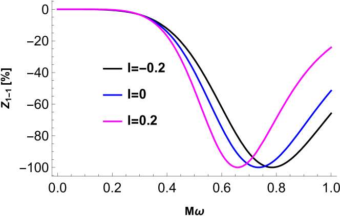
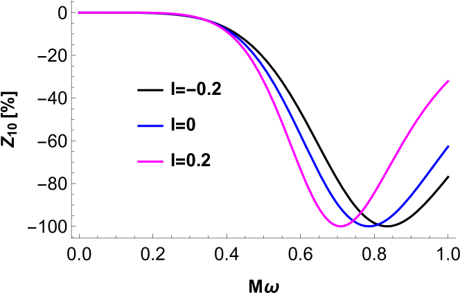
Figure 5: Variation of amplification factors with $\ell$ for non-superradiant multipoles with $\hat{\mu}=0.1,b=0.1$, and $\hat{a}=0.4$.

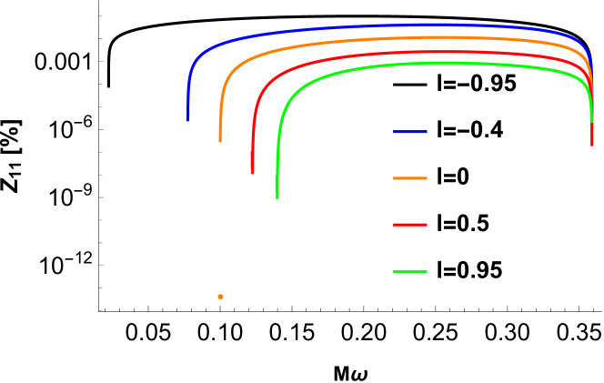
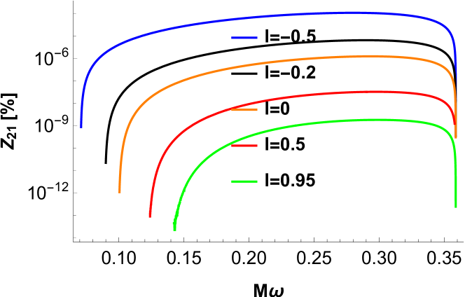
Figure 6: Variation of amplification factors with $\ell$ for various multipoles with $\hat{\mu}=0.1,b=0.1$, and $\hat{a}=0.9$.

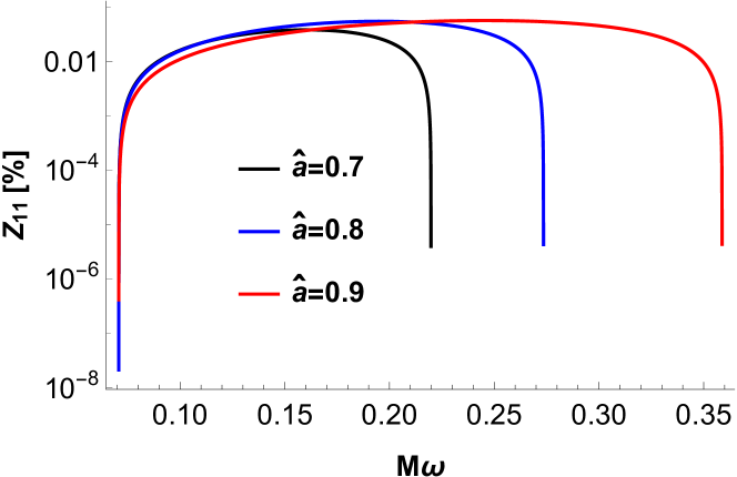
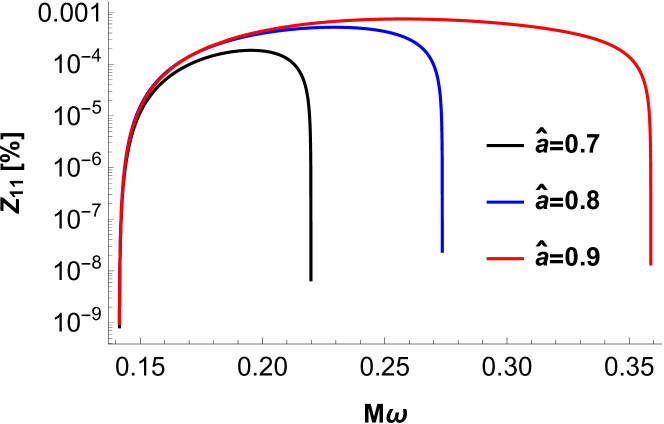
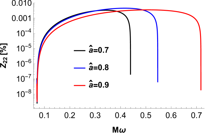
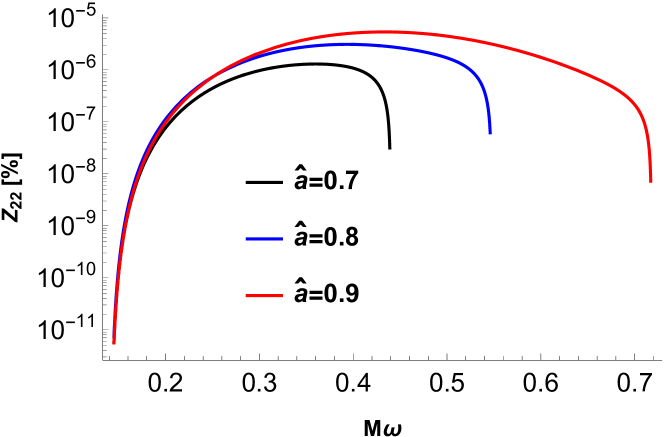
Figure 7: Variation of amplification factors with $\hat{a}$ for various multipoles with $\hat{\mu}=0.1$ and $b=0.1$. For left ones $\ell=-0.5$ and for right ones $\ell=1$.

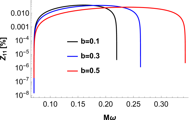
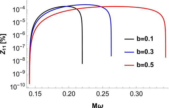
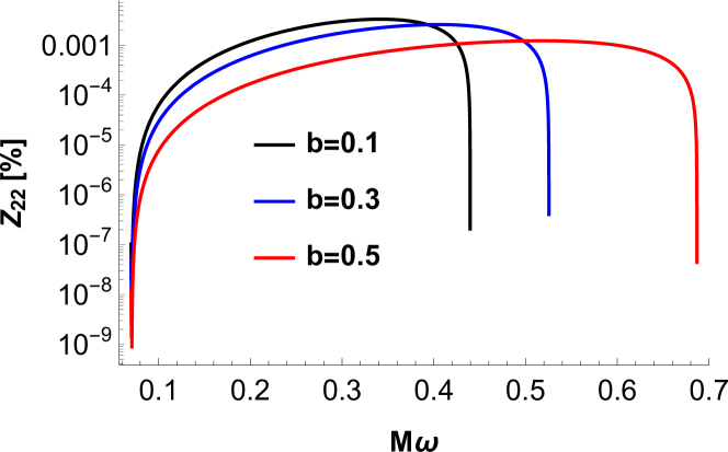
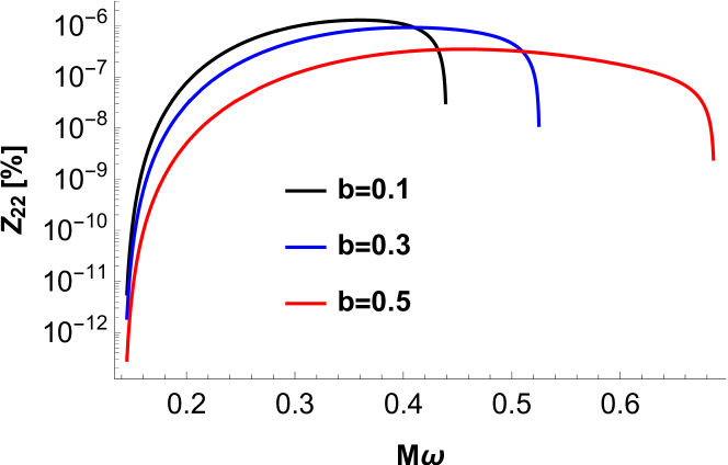
Figure 8: Variation of amplification factors with $b$ for various multipoles with $\hat{\mu}=0.1$ and $\hat{a}=0.7$. For left ones $\ell=-0.5$ and for right ones $\ell=1$.

IV.1 Superradiant instability for Kerr-Sen-like black hole

From equation (15) we have

$$\Delta\frac{d}{dr}\left(\Delta\frac{dR_{\omega jm}}{dr}\right)+\xi R_{\omega jm}=0,$$ (43)

where for a slowly rotating black hole $(\hat{a}\omega\ll 1)$

$$\xi\equiv\frac{\left(\left(r(r+b)+\hat{a}^{2}\right)\omega-m\hat{a}\right)^{2}}{1+\ell}+\Delta\left(2m\hat{a}\omega-l(l+1)-\mu^{2}r(r+b)\right).$$

Demanding the black hole bomb mechanism, we should have the following solutions for the radial equation (43)

$$R_{\omega jm}\sim\left\{\begin{array}[]{ll}e^{-i(\omega-m\hat{\Omega})r_{*}}&\text{ as }r\rightarrow r_{eh}\left(r_{*}\rightarrow-\infty\right)\\ \frac{e^{-\sqrt{\mu^{2}-\omega^{2}r_{*}}}}{r}&\text{ as }r\rightarrow\infty\left(r_{*}\rightarrow\infty\right)\end{array}\right.$$

The above solution represents the physical boundary conditions that the scalar wave at the black hole horizon is purely ingoing while at spatial infinity it is decaying exponentially (bounded) solution, provided that $\omega^{2}<\mu^{2}$. With the new radial function

$$\psi_{\omega jm}\equiv\sqrt{\Delta}R_{\omega jm},$$

the radial equation (43) becomes

$$\left(\frac{d^{2}}{dr^{2}}+\omega^{2}(1+\ell)-V\right)\psi_{\omega jm}=0.$$

with

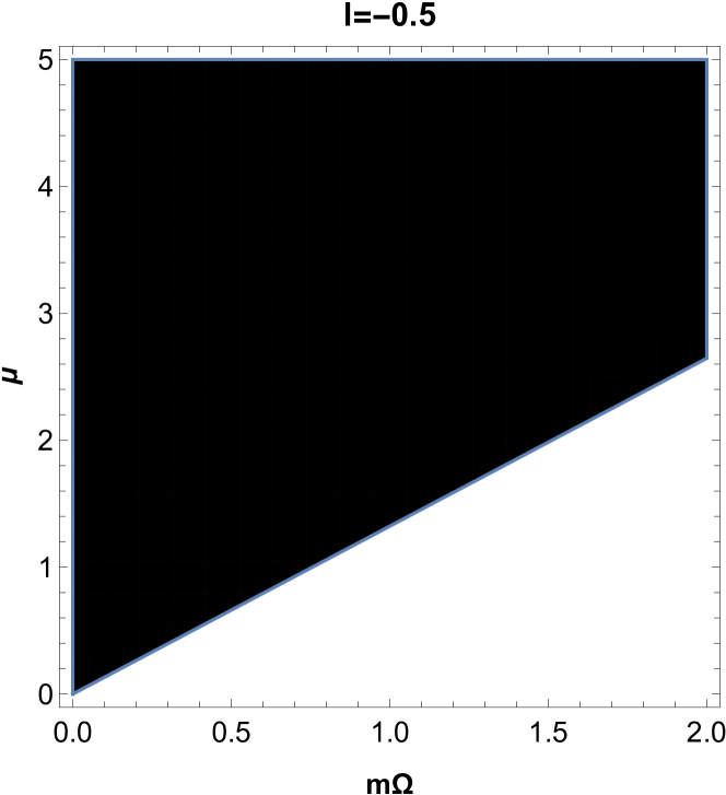
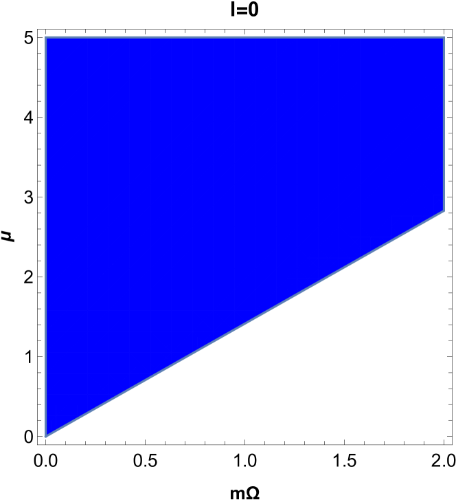
Figure 9: Parameter space($m\Omega$-$\mu$) for massive scalar field where colored area represents region with stable dynamics and non-colored area represents region with unstable dynamics.

$$\omega^{2}(1+\ell)-V=\frac{\xi\left(1+\ell\right)+M^{2}-\hat{a}^{2}+\frac{b^{2}}{4}-bM}{\Delta^{2}},$$

which is the Regge-Wheel equation. By discarding the terms $\mathcal{O}\left(1/r^{2}\right)$ the asymptotic form of the effective potential $V(r)$ reads

$$V(r)=\mu^{2}\left(1+\ell\right)-\left(1+\ell\right)\frac{4M\omega^{2}}{r}+(\ell+1)\frac{2M\mu^{2}}{r}.$$

To realize the trapping meaningfully by the above effective potential it is necessary that its asymptotic derivative be positive i.e. $V^{\prime}\rightarrow 0^{+}$ as $r\rightarrow\infty[33]$. This along with the fact that superradiance amplification of scattered waves occur when $\omega<m\hat{\Omega}$ we get the regime

$$\frac{\mu}{\sqrt{2}}<\omega^{2}<m\hat{\Omega},$$

in which the integrated system of Kerr-Sen bumblebee black hole and massive scalar field may experience a superradiant instability, known as the black hole bomb. The dynamics of the massive scalar field in Kerr-Sen like black hole will remain stable when $\mu\geq\sqrt{2}m\hat{\Omega}$.

V Constraining from the observed data for $\mathrm{M}87^{*}$

This section is devoted to constraining the parameters from the observed data for $\mathrm{M}87^{*}$. After the announcement of the capturing of the shadow there have been several attempts to constraint the parameters used in different modified theories of gravity MISBAM87 ; MK ; SGM87 . However, before going towards constraining parameters let us give a brief description of the photon orbit in this Kerr-Sen-like spacetime background and see how the shadow gets deformed with the additional parameters of this Lorentz violating spacetime.

V.1 Mathematical formulation of the deviation from circularity

The Hamiltonian for a massless particle like the photon is given by

$$H\left(x^{\tau},p_{\tau}\right)=\frac{1}{2}\left[g^{\tau\nu}p_{\tau}p_{\nu}-\left(p_{0}\sqrt{-g^{00}}\right)^{2}\right].$$ (44)

The standard definitions $x^{\tau}=\partial H/\partial p_{\tau}$, and $\dot{p_{\tau}}=\partial H/\partial x^{\tau}$ renders the equations of motion for the photon. Then the null geodesics in the bumblebee rotating black hole spacetime in terms of $\xi$ are given by

$$\rho^{2}\frac{dr}{d\lambda}=\pm\sqrt{R},\qquad\rho^{2}\frac{d\theta}{d\lambda}=\pm\sqrt{\Theta},$$

$$(1+\ell)\Delta\rho^{2}\frac{dt}{d\lambda}=A-2\sqrt{1+\ell}\operatorname{Mra\xi},$$

$$(1+\ell)\Delta\rho^{2}\frac{d\phi}{d\lambda}=2\sqrt{1+\ell}Mra+\frac{\xi}{\sin^{2}\theta}\left(\rho^{2}-2Mr\right),$$ (45)

where $\lambda$ is the affine parameter and

$$R(r)=\left[\frac{r(r+b)+(1+\ell)a^{2}}{\sqrt{1+\ell}}-a\xi\right]^{2}-\Delta\left[\eta+(\xi-\sqrt{1+\ell}a)^{2}\right],\Theta(\theta)=\eta+(1+\ell)a^{2}\cos^{2}\theta-\xi^{2}\cot^{2}\theta.$$ (46)

In the Eqns. (45) and (46), we introduce two conserved parameters $\xi$ and $\eta$ as usual which are defined by

$$\xi=\frac{L_{z}}{E}\quad\textrm{and}\quad\eta=\frac{\mathcal{Q}}{E^{2}},$$ (47)

where $E$, $L_{z}$, and $\mathcal{Q}$ are the energy, the axial component of the angular momentum, and the $Carter~{}constant$ respectively. The radial equation of motion can be cast into the known form

$$\left(\rho^{2}\frac{dr}{d\lambda}\right)^{2}+V_{eff}=0.$$ (48)

The effective potential $V_{eff}$ in this situation is written down as

$$V_{eff}=-[\frac{r(r+b)+(1+l)a^{2}}{\sqrt{1+l}}-a\xi]^{2}+\Delta\left[\eta+(\xi-\sqrt{1+l}a)^{2}\right]-\frac{\left[r(r+b)+a^{2}(1+l)\right]^{2}}{1+l}.$$ (49)

Note that it has explicit dependence on the LV factor $\ell$ and $a$. So it is natural that the structure the of photon orbit will depend on the parameters $a$ and $l$. The unstable spherical orbit on the equatorial plane is given by the following equations

$$\theta=\frac{\pi}{2},\quad R(r)=0,\quad\frac{dR}{dr}=0,\quad\frac{d^{2}R}{dr^{2}}<0,\quad\mathrm{and}\quad\eta=0.$$ (50)

For more generic orbits $\theta\neq\pi/2$ and $\eta\neq 0,$ the solution of Eqn. (50) $r=r_{s}$, gives the $r-$ constant orbit, which is also called spherical orbit and the conserved parameters of the spherical orbits can be expressed in the following form

$$\begin{aligned} \xi_{s}&=\frac{a^{2}\left(1+\mathrm{l}\right)\left(2M+2r_{\mathrm{s}}+b\right)+r_{\mathrm{s}}\left(2r_{\mathrm{s}}^{2}+3br_{\mathrm{s}}+b^{2}-2M\left(3r_{\mathrm{s}}+b\right)\right)}{a\sqrt{1+\mathrm{l}}\left(2M-2r_{\mathrm{s}}-b\right)},\\ \eta_{s}&=-\frac{r_{\mathrm{s}}^{2}\left(-8a^{2}\left(1+\mathrm{l}\right)M\left(2r_{\mathrm{s}}+b\right)+\left(2r_{\mathrm{s}}^{2}+3br_{\mathrm{s}}+b^{2}-2M\left(3r_{\mathrm{s}}+b\right)\right)^{2}\right)}{a^{2}\left(1+\mathrm{l}\right)\left(2M-2r_{\mathrm{s}}-b\right)^{2}}.\end{aligned}$$ (51)

The two celestial coordinates which are used to describe the shape of the shadow that an observer see in the sky, can be given by

$$\alpha(\xi,\eta;\theta) = \lim_{r\rightarrow\infty}\frac{-rp^{(\varphi)}}{p^{(t)}}=-\xi_{s}\csc\theta,$$

$$\beta(\xi,\eta;\theta) = \lim_{r\rightarrow\infty}\frac{rp^{(\theta)}}{p^{(t)}}=\sqrt{\left(\eta_{s}+a^{2}\cos^{2}\theta-\xi_{s}^{2}\cot^{2}\theta\right)},$$

where $(p^{(t)},p^{(r)},p^{(\theta)}$, and $p^{(\phi)})$ are the tetrad components of the photon momentum with respect to locally non-rotating reference frames BARDEEN .

V.2 Constraining with respect to deviation from circularity data: $\Delta C\leq 0.10$

We now proceed towards constraining the parameters involved in this spacetime metric from the available experimental findings of the $M87^{*}$ as a new window for testing gravity in the strong-field regime has been opened after the announcement of the news of capturing the image of supermassive black hole $M87^{*}$ at $1.3mm$ wavelength with the angular resolution of $20\mu as$. The angular diameter of the shadow of $M87^{*}$ was fund to be $\theta_{d}=42\pm 3\mu as$ and the deviation from circularity was $\Delta C\leq 10$ which was consistent with the Kerr black hole’s image as predicted from the theory of General Relativity EHT1 ; EHT2 ; EHT3 ; EHT4 ; EHT5 ; EHT6 . Let us first proceed to constrain the parameter from the observation of $M87^{*}$ concerning $\Delta C\leq.10$. We have considered Kerr-Sen-like black holes, which have additional parameters $b$, $l$ along with the Kerr black hole parameters, and the parameters $b$ and $l$ produce deviation from Kerr geometry with a considerably good configuration. It is also found that the LV parameter quantitatively influences the structure of the event horizon by reducing its radius significantly than that of the Kerr black hole ARS , for a given $b$ and $a$, and the resulting increase in ergosphere area is thereby likely to have an impact on energy extraction ARS . The boundary of the shadow is described by the polar coordinate $(R(\phi),\phi)$ with the origin at the center of the shadow $(\alpha_{C},\beta_{C})$, where $\alpha_{C}=\frac{|\alpha_{max}+\alpha_{min}|}{2}$ and $\beta_{C}=0$. If a point $(\alpha,\beta)$ over the boundary of the image subtends an angle $\phi$ on the $\alpha$ axis at the geometric center, $\left(\alpha_{C},0\right)$ and $R(\phi)$ be the distance between the point $(\alpha,\beta)$ and $\left(\alpha_{C},0\right)$, then the average radius $R_{\text{avg}}$ of the image is given by CBK

$$R_{\text{avg}}^{2}\equiv\frac{1}{2\pi}\int_{0}^{2\pi}d\phi R^{2}(\phi),\\$$ (53)

where $R(\phi)\equiv\sqrt{\left(\alpha(\phi)-\alpha_{C}\right)^{2}+\beta(\phi)^{2}}$, and $\phi=tan^{-1}\frac{\beta(\phi)}{\alpha(\phi)-\alpha_{C}}$

With the above inputs, the circularity deviation $\Delta C$ is defined by TJDP ,

$$\Delta C\equiv 2\sqrt{\frac{1}{2\pi}\int_{0}^{2\pi}d\phi\left(R(\phi)-R_{\text{avg }}\right)^{2}}.$$ (54)

In the figures below, the deviation from circularity $\Delta C$ is shown for Kerr-Sen-like black holes for inclination angles $\theta=90^{o}$ and $17^{o}$ respectively.

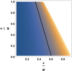
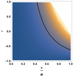
Figure 10: The left one is for $\ell=0.1$ and the right one is for $b=0.1$ where the inclination angle is $90^{o}$. The black solid lines correspond to $\Delta C=0.1$.

     

Figure 11: The left one is for $\ell=0.1$ and the right one is for $b=0.1$ where the inclination angle is $17^{o}$.

We compare the shadows produced from the numerical calculation by the Kerr-Sen-like black holes with the observed one for the $\mathrm{M}87^{*}$ black hole. For comparison, we consider the experimentally obtained astronomical data for the circularity deviation $\Delta\leq 0.10$ in this subsection. The next section is devoted to constrain the parameter from observation of angular diameter $\theta_{d}=42\pm 3\mu as$ EHT1 ; EHT2 ; EHT3 ; EHT4 ; EHT5 ; EHT6 .

V.3 Constraining from the observation of angular diameter $\theta_{d}=42\pm 3\mu as$

We now consider the shadow angular diameter which is define by

$$\theta_{d}=\frac{2}{d}\sqrt{\frac{A}{\pi}},$$ (55)

Where $A=2\int_{r_{-}}^{r_{+}}\beta d\alpha$ is the shadow area and $d=16.8Mpc$ is the distance of $M87^{*}$ from the earth. These relations enable us to accomplish a comparison between the theoretical predictions for Kerr-Sen-like black-hole shadows and the experimental findings of the Event Horizon Telescope collaboration. In the figures below, the angular diameter $\theta_{d}$ is shown for Kerr-Sen-like black holes for inclination angles $\theta=90^{o}$ and $17^{o}$ respectively.

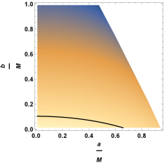
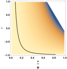
Figure 12: The left one is for $\ell=0.1$ and the right one is for $b=0.1$ where the inclination angle is $90^{o}$.The black solid lines correspond to $\theta_{d}=39\mu as$.

     

Figure 13: The left one is for $\ell=0.1$ and the right one is for $b=0.1$ where the inclination angle is $17^{o}$.The black solid lines correspond to $\theta_{d}=39\mu as$.

VI Summary and discussions

In this article, we have studied the superradiance phenomena of the scalar field scattered off Kerr-sen-like black holes along with the study of some salient features of the Kerr-sen-like Lorentz violating spacetime. The LV parameter enters into the Kerr-Sen-like background via a spontaneous symmetry breaking when the pseudovector field of the bumblebee field receives a vacuum expectation value. The Kerr-Sen-like spacetime is a solution to Einstein’s bumblebee gravity model. Along with the parameter $M$, $a$ (which are contained in the Kerr spacetime metric) the Kerr-Sen-like metric has two more parameters, $b$ and the LV parameter $\ell$.The presence of these four parameters has a crucial role in the spacetime geometry associated with the matric. Depending on the value of the parameter we can have non-extremal and extremal cases. We can even have a naked singularity. We observed that the parameter space formed by $a$ and $b$ that corresponds to black hole singularity is getting reduced with an increase in the value of the LV parameter. We have also observed that the size of the ergosphere gets enhanced with the increase in the value LV parameter. The increase in the value of $b$ also results in an increase in the size of the ergosphere like the increase in the value of $\ell$.

If we look towards the superradiance phenomena of the scalar field scattered off Kerr-sen-like black holes we find that the LV effect has a great influence on the superradiance phenomena. How the superradiance phenomena and the instability associated with it get influenced by the Lorentz violation effect is studied in detail. We consider the Klein-Gordon equation in the Kerr-Sen-like background and employ asymptotic matching of the scalar wave, and establish transparently from the equation (25) that in the low-frequency limit, i.e., for $\omega<m\hat{\Omega}_{eh}$, the scalar waves show the superradiant mode, i.e. it becomes amplified in a superradiant manner. The numerical computation, however, shows that for $m\leq 0$ the massive scalar field has a non-superradiant mode. For $m\geq 0$ it is superradiant. The role of the LV parameter in the superradiant phenomena as we have observed is as follows. The superradiant process enhances with the decrease in the value of the LV parameter and reverse is the case when the LV parameter increases irrespective of the sign of the value of this parameter please vide Fig.6.

Our observation also transpires that the superradiant process gets influenced by the parameter $b$ also. From Fig. 8, it is clear that the superradiance enhances with the decrease of the positive value of the parameter $b$. Note that $b=\frac{Q^{2}}{M}$. So it cannot be negative.

Extending the issue of the black hole bomb, the analytical study of superradiant instability is made. Fig. 9 related to the study of superradiant instability reveals that the LV parameter remarkably affects the instability regime. In the background with negative LV Parameter, the scalar field has more chances to acquire unstable dynamics and for the positive values of the LV parameter, these chances are less. Therefore, the LV has a significant influence on the superradiance scattering phenomena and the corresponding instability linked with it.

In his article we have also tried to put constraints on parameters contained in the Kerr-Sen-like spacetime metric from the observation of $M87^{*}$, and observed that the circularity deviation $\delta C\leq 0.1$ EHT1 ; EHT2 ; EHT3 ; EHT4 ; EHT5 ; EHT6 is satisfied exhaustively for the entire $(a-l)$ and $(b-l)$ parameter space at $\theta=17^{0}$ inclination angle but at inclination angle $\theta=90^{0}$ it is satisfied for a finite $(a-l)$ and $(b-l)$ space. The angular diameter satisfies $\theta_{d}=42\pm 3\mu as$ within the $1\sigma$ region EHT1 ; EHT2 ; EHT3 ; EHT4 ; EHT5 ; EHT6 over a finite $(a-b)$ and $(a-l)$ space. However, when we compare with angular diameter $\theta_{d}=42\pm 3\mu as$ data it is found that agreeable $(a-b)$ parameter space is smaller than the $(a-l)$ parameter space and it is more restricted.

Besides we should make some comments in connection with the recent article MALUF . The comment of the article although does not target our study of superradiance directly, the $b=0$ limit of our metric has to pass through this unfavorable situation. In fact, the comment made in MALUF is all about the inconsistency of the black hole solution obtained in DING which is a special case: b=0 of the metric used here. Even if that inconsistency is taken as granted in the metric developed in DING , it has been pointed out in the article KANGI , that in the slow rotating limit $a\rightarrow 0$ the metric has a consistent outcome. With this limit, the metric turns into a true slowly rotating black hole solution of Einstein-bumblebee gravity DINGC . Moreover, for $a=b=0$, one lands onto the flawless Schwarzschild-like solution of the Einstein-bumblebee gravity presented in CASANA .

Appendix-A

Following the procedure as followed in BEZERRA the general solution of equation (15) is given by

$$R(z)=\frac{M}{\sqrt{\Delta(1+1)}}e^{\frac{1}{2}\alpha z}(z-1)^{\frac{1}{2}(1+\gamma)}z^{\frac{1}{2}(1+\beta)}\times$$ (56)

$$\left\{C_{1}\text{HeunC }(\alpha,\beta,\gamma,\delta,\eta,z)+C_{2}z^{-\beta}\text{ HeunC }(\alpha,-\beta,\gamma,\delta,\eta,z)\right\}$$

with

$$2Md=r_{+}-r_{-},z=-\frac{1}{2Md}(r-r_{+})$$

$$\alpha=4dM\left(\mu^{2}-\omega^{2}\right)^{1/2}\sqrt{1+l}$$

$$\beta=\sqrt{1-\frac{4A}{M^{2}}},$$

$$\gamma=\sqrt{1-\frac{4C}{M^{2}}},\delta=-\frac{2d}{M^{2}}(B+D)$$

$$\eta=\frac{1}{2}+\frac{2Bd}{M^{2}}$$

where

$$A =\frac{1}{4d^{2}}\left[4M^{4}\omega^{2}(1+l)(d+1)^{2}+\left(Mb-\frac{b^{2}}{4}\right)\omega^{2}(1+l)+\hat{a}^{2}m^{2}(1+l)\right.$$

$$+4\hat{a}\omega mMb(1+l)+M^{2}d^{2}+\left(2Mb\omega^{2}\left(Mb-\frac{b^{2}}{4}\right)(1+l)\right.$$

$$\left.-4M^{2}\left(Mb-\frac{b^{2}}{4}\right)\omega^{2}(1+l)-4\hat{a}\omega mM^{2}(1+l)\right)(d+1)$$

$$\left.+\left(M^{2}b^{2}-4M^{3}b\right)\omega^{2}(d+1)^{2}(1+l)\right]$$

$$B =\frac{1}{4d^{3}}\left[4M^{4}\omega^{2}(d+1)^{2}(2d-1)(1+l)+\left(M^{2}b^{2}-4M^{3}b\right)\omega^{2}\left(d^{2}-1\right)(1+l)\right.$$

$$-\left(Mb-\frac{b^{2}}{4}\right)\omega^{2}(1+l)-\hat{a}^{2}m^{2}(1+l)-4\hat{a}\omega mMb(1+l)-M^{2}d^{2}$$

$$-\left(2Mb\omega^{2}\left(Mb-\frac{b^{2}}{4}\right)(1+l)-4M^{2}\left(Mb-\frac{b^{2}}{4}\right)\omega^{2}(1+l)\right.$$

$$-\left.4\hat{a}\omega mM^{2}(1+l)\right)+2d^{2}(d+1)\left(-2M^{3}b\omega^{2}(1+l)\right.$$

$$\left.+\mu^{2}M^{3}b(1+l)\right)+2d^{2}\left(-2M^{2}\omega^{2}(1+l)\left(Mb-\frac{b^{2}}{4}\right)\right.$$

$$-\left.\left.\mu^{2}M^{4}(d+1)^{2}(1+l)-\left(\hat{a}^{2}\omega^{2}+j(1+j)\right)M^{2}(1+l)\right)\right]$$

$$C =\frac{1}{4d^{2}}\left[4M^{4}\omega^{2}(d-1)^{2}(1+l)+\left(M^{2}b^{2}-4M^{3}b\right)\omega^{2}(d-1)^{2}(1+l)\right.$$

$$+\left(Mb-\frac{b^{2}}{4}\right)\omega^{2}(1+l)+\hat{a}^{2}m^{2}(1+l)+4\hat{a}\omega mMb(1+l)+M^{2}d^{2}$$

$$-(d-1)\left(2Mb\omega^{2}\left(Mb-\frac{b^{2}}{4}\right)(1+l)-4M^{2}\left(Mb-\frac{b^{2}}{4}\right)\omega^{2}(1+l)\right.$$

$$\left.\left.-4\hat{a}\omega mM^{2}(1+l)\right)\right]$$

$$D =\frac{1}{4d^{3}}\left[4M^{4}\omega^{2}(d-1)^{2}(2d+1)(1+l)-\left(d^{2}-1\right)\left(M^{2}b^{2}-4M^{3}b\right)\omega^{2}(1+l)\right.$$

$$+\left(Mb-\frac{b^{2}}{4}\right)\omega^{2}(1+l)+\hat{a}^{2}m^{2}(1+l)+4\hat{a}\omega mMb(1+l)+M^{2}d^{2}$$

$$+2Mb\omega^{2}\left(Mb-\frac{b^{2}}{4}\right)(1+l)-4M^{2}\left(Mb-\frac{b^{2}}{4}\right)\omega^{2}(1+l)$$

$$-4\hat{a}\omega mM^{2}(1+l)+2d^{2}(d-1)\left(-2M^{3}b\omega^{2}(1+l)\right.$$

$$\left.+\mu^{2}M^{3}b(1+l)\right)+2d^{2}\left(2M^{2}\omega^{2}(1+l)\left(Mb-\frac{b^{2}}{4}\right)\right.$$

$$\left.\left.+\mu^{2}M^{4}(d+1)^{2}(1+l)+\left(\hat{a}^{2}\omega^{2}+j(1+j)\right)M^{2}(1+l)\right)-2\mu^{2}M^{4}(1+l)\right]$$

In the limit $z\rightarrow 0\Rightarrow r\rightarrow r_{+}$ we have

$$R(r)=\frac{M}{\sqrt{\Delta(1+1)}}\left[C_{1}\left\{-\frac{1}{2Md}\left(r-r_{+}\right)\right\}^{\frac{1}{2}(1+\beta)}+C_{2}\left\{-\frac{1}{2Md}\left(r-r_{+}\right)\right\}^{\frac{1}{2}(1-\beta)}\right]\text{,}$$

and in the limit $z\rightarrow\infty\Rightarrow r\rightarrow\infty$ we land onto

$$R(r) =\frac{M}{\sqrt{\Delta(1+l)}}\left[C_{1}e^{-i\sqrt{\omega^{2}-\mu^{2}}\sqrt{l+l}\left(r-r_{+}\right)}z^{k}\right.$$

$$\left.+C_{2}e^{i\sqrt{\omega^{2}-\mu^{2}}\sqrt{1+l}\left(r-r_{+}\right)}z^{-k}\right]$$

where

$$k=-\delta/\alpha$$

The solution of near and far region should agree with the solution used hare in our study of superradence. However it is an involved mathematical issue and it is beyond the scope of this article.

References

- (1) Y. B. Zel’dovich Pis’ma Zh. Eksp. Teor. Fiz. 14 (1971) 270 [JETP Lett. 14, 180 (1971)].
- (2) Y. B. Zel’dovich Zh. Eksp. Teor. Fiz 62 (1972) 2076 [Sov.Phys. JETP 35, 1085 (1972)].
- (3) R. Brito, V. Cardoso, P. Pani: Lecture Notes in Physics (2nd edition) 971 (2020)
- (4) S. Hawking, Commun.Math.Phys. 43 (1975) 199
- (5) A. Arvanitaki, S. Dimopoulos, S. Dubovsky, N. Kaloper, and J. March-Russell, Phys.Rev. D81(2010) 123530,
- (6) A. Arvanitaki,S. Dubovsky, Phys.Rev. D83 (2011) 044026,
- (7) P. Pani, V. Cardoso, L. Gualtieri, E. Berti, A. Ishibashi, Phys.Rev.Lett. 109 (2012) 131102,
- (8) R. Brito, V. Cardoso, P. Pani, Phys. Rev. D88 (2013) 023514
- (9) C. A. R. Herdeiro and E. Radu, Phys.Rev.Lett. 112 (2014) 221101,
- (10) V. Cardoso and O. J. Dias, Phys.Rev. D70 (2004) 084011,
- (11) O. J. Dias, P. Figueras, S. Minwalla, P. Mitra, R. Monteiro, et al. JHEP 1208(2012) 117
- (12) O. J. Dias, G. T. Horowitz, and J. E. Santos, JHEP 1107 (2011) 115,
- (13) M. Shibata and H. Yoshino, Phys. Rev. D81 (2010) 104035,
- (14) P. Pani, C. F. B. Macedo, L. C. B. Crispino and V. Cardoso, Phys. Rev. D 84 (2011) 087501
- (15) B. Kleihaus, J. Kunz and E. Radu, Phys. Rev. Lett. 106 (2011) 151104
- (16) T. Delsate, C. Herdeiro and E. Radu, Phys. Lett. B787 (2018) 8
- (17) P. V. P. Cunha, C. A. R. Herdeiro and E. Radu, Phys. Rev. Lett. 123 (2019) 011101
- (18) V. Cardoso, I. P. Carucci, P. Pani and T. P. Sotiriou, Phys. Rev. D88 (2013) 044056
- (19) V. Cardoso, I. P. Carucci, P. Pani and T. P. Sotiriou, Phys. Rev. Lett. 111 (2013) 111101
- (20) A. N. Aliev, JCAP 1411 (2014) 029
- (21) C. Y. Zhang, S. J. Zhang and B. Wang, JHEP 1408 (2014) 011
- (22) O. Fierro, N. Grandi and J. Oliva, Class. Quant. Grav. 35 (2018) 105007
- (23) M. F. Wondrak, P. Nicolini and J. W. Moffat, JCAP 1812 (2018) 021
- (24) T. Kolyvaris, M. Koukouvaou, A. Machattou and E. Papantonopoulos, Phys. Rev. D 98 (2018) 024045
- (25) A. Rahmani, M. Honardoost and H. R. Sepangi, Phys. Rev. D 101 (2020) 084036
- (26) M. Khodadi, A. Talebian and H. Firouzjahi, arXiv:2002.10496
- (27) C. Y. Zhang, S. J. Zhang, P. C. Li M. Guo, JHEP 2008 (2020) 105
- (28) V. A. Kostelecky, Phys. Rev. D 69 (2004) 105009
- (29) V. A. Kostelecky and R. Potting, Phys. Lett. B 381 (1996) 89
- (30) D. Colladay and V. A. Kostelecky, Phys. Rev. D 55 (1997) 6760
- (31) D. Colladay and V. A. Kostelecky, Phys. Rev. D 58 (1998) 116002
- (32) S. R. Coleman and S. L. Glashow, Phys. Rev. D 59 (1999) 116008
- (33) M. D. Seifert, Phys. Rev. D 81 (2010) 065010
- (34) J. Paramos and G. Guiomar, Phys. Rev. D 90 (2014) 082002
- (35) D. Capelo and J. Paramos, Phys. Rev. D 91 (2015) 104007
- (36) R. Oliveira, D. M. Dantas, V. Santos and C. A. S. Almeida, Class. Quant. Grav. 36 105013 (2019)
- (37) A. Ovgun, K. Jusufi, I. Sakalli, Annals Phys. 399 (2018) 193
- (38) A. Ovgun, K. Jusufi, I. Sakalli, Phys. Rev. D99 (2019) 024042
- (39) R. Oliveira, D. M. Dantas, C. A. S. Almeida EPL 135 10003 2021
- (40) C. Ding, C. Liu, R. Casana, A. Cavalcante: Eur. Phys. J. C 80 (2020) 178
- (41) R. Casana, A. Cavalcante, F. P. Poulis and E. B. Santos, Phys. Rev. D97 104001 (2018)
- (42) S. K. Jha, A. Rahaman: Eur.Phys.J. C81 (2021) 345
- (43) S. K. Jha, H. Barnan A. Rahaman:JCAP 2104 (2021) 036
- (44) S. K. Jha, S. Aziz: A Rahaman:arXiv:2103.17021 (2021), to appear in Eur. Phys. J
- (45) A. Sen: Phys.Rev.Lett. 69 1006 (1992)
- (46) M. Khodadi: Phys.Rev. D103, 064051 (2021)
- (47) S. U. Islam, S. G. Ghosh: Phys. Rev. D 103, 124052 (2021)
- (48) S. G. Ghosh , M. Amir, S. D. Maharaj: Nucl. Phys.B957,115088 (2020)
- (49) M. Amir, B. P. Singh, S. G. Ghosh: Eur. Phys. J. C78, 399 (2018)
- (50) T. Johannsen and D. Psaltis, Astrophys. J. 718, 446 (2010).
- (51) R. Penrose, Riv. Nuovo Cim. 1, 252 (1969).
- (52) R. Penrose, M. R. Floyd: Nature, 229, 177 (1971)
- (53) V. B. Bezerra , H. S. Vieira and A. A. Costa: Class.Quantum Grav. 31 045003 (2014)
- (54) G. V. Kraniotis: Class.Quant.Grav. 33 225011 (2016)
- (55) S. Q. Wu J. Math. Phys. 44, 1084 (2003)
- (56) Ran Li: Phys. Lett. B714 337 (2012)
- (57) A. A. Starobinsky, Zh. Eksp. Teor. Fiz. 64, 48 (1973) [Sov.Phys. JETP 37, 28 ( 1973)]
- (58) A. A. Starobinsky and S. M. Churilov: Zh. Eksp. Teor. Fiz. 65, 3 (1973) [Sov. Phys. JETP 38, 1 (1973)].
- (59) S. A. Teukolsky, W. H. Press: Astrophys. J. 193 443 (1974)
- (60) D. N. Page: Phys. Rev. D13 198 (1976)
- (61) C. Bambi, K. Freese, S. Vagnozzi, L. Visinelli, Phys.Rev.D100(4):044057(2019).
- (62) S. G. Ghosh , R. Kumara, S. U. Islama: JCAP, 03, 056 (2021)
- (63) M. Afrin, R. Kumar, S. G. Ghosh MNRAS 504 5927 (2021)
- (64) S. G. Ghosh, R. Kumar, S. U. Islam JCAP03 056 (2021)
- (65) J. M. Bardeen, W. H. Press and S. A. Teukolsky, Astro-phys. J. 178, 347 (1972).
- (66) K. Akiyama et al. (Event Horizon Telescope Collaboration), First M87 Event Horizon Telescope results. I. The shadow of the supermassive black hole, Astrophys. J. 875, L1 (2019).
- (67) K. Akiyama et al. (Event Horizon Telescope Collaboration), First M87 Event Horizon Telescope results. II. Array and instrumentation, Astrophys. J. 875, L2 (2019).
- (68) K. Akiyama et al. (Event Horizon Telescope Collaboration), First M87 Event Horizon Telescope results. III. Data processing and calibration, Astrophys. J. 875, L3 (2019).
- (69) K. Akiyama et al. (Event Horizon Telescope Collaboration), First M87 Event Horizon Telescope results. IV. Imaging the central supermassive black hole, Astrophys. J. 875, L4 (2019).
- (70) K. Akiyama et al. (Event Horizon Telescope Collaboration), First M87 Event Horizon Telescope results. V. Physical origin of the asymmetric ring, Astrophys. J. 875, L5 (2019).
- (71) K. Akiyama et al. (Event Horizon Telescope Collaboration), First M87 Event Horizon Telescope results. VI. The shadow and mass of the central black hole, Astrophys. J. 875, L6 (2019)
- (72) R.V. Maluf, C.R Muniz:Eur.Phys.J.C 82 1, 94 (2022)
- (73) S. Kanzi, I. Sakall: Eur. Phys. J. C 82:93 (2022)
- (74) C. Ding, X. Chen, Chin. Phys. C 45(2), 025106 (2021)