Final m/s version of paper published in Neural Computation 34(10) 2037-2046 (2022), with an addendum (arXiv only) added in March 2023. On Suspicious Coincidences and
Pointwise Mutual Information

Abstract

Barlow, (1985) hypothesized that the co-occurrence of two events $A$ and $B$ is ‘suspicious’ if $P(A,B)\gg P(A)P(B)$. We first review classical measures of association for $2\times 2$ contingency tables, including Yule’s $Y$ (Yule,, 1912), which depends only on the odds ratio $\lambda$, and is independent of the marginal probabilities of the table. We then discuss the mutual information (MI) and pointwise mutual information (PMI), which depend on the ratio $P(A,B)/P(A)P(B)$, as measures of association. We show that, once the effect of the marginals is removed, MI and PMI behave similarly to $Y$ as functions of $\lambda$. The pointwise mutual information is used extensively in some research communities for flagging suspicious coincidences. We discuss the pros and cons of using it in this way, bearing in mind the sensitivity of the PMI to the marginals, with increased scores for sparser events.

Barlow, (1985) hypothesized that “the cortex behaves like a gifted detective, noting suspicious coincidences in its afferent input, and thereby gaining knowledge of the non-random, causally related, features in its environment”. More specifically, Barlow wrote (p. 40):

The coincident occurrence of two events $A$ and $B$ is ‘suspicious’ if they occur jointly more than would be expected from the probabilities of their individual occurrence, i.e. the coincidence $A\&B$ is suspicious if $P(A\&B)\gg P(A)\times P(B)$. Any detective knows that, for a coincidence to be suspicious, the events themselves must be rare ones, and that if they are rare enough, even a single occurrence is significant.

Edelman et al., (2002) refer to the principle of suspicious coincidences as where “two candidate fragments $A$ and $B$ should be combined into a composite object if the probability of their joint appearance $P(A,B)$ is much higher than $P(A)P(B)$ …”

The fundamental problem here is to detect if there is a significant association between events $A$ and $B$. This can arise in many different contexts, such as:

• an animal detecting that eating a certain plant is associated with subsequent illness;

• detecting that a certain drug is associated with a particular adverse drug reaction;

• detecting the association between a visual stimulus that contains an image of the subject’s grandmother or not, and the response of a putative “grandmother cell”;

• detecting that particular successive words in text are associated more frequently than by chance—this is called a “collocation”, an example being the bigram “carbon dioxide”;

• a geneticist determining that two genes are in linkage disequilibrium (see e.g., Lewontin, 1964);

• detecting that the pattern of two edges in a visual scene making a corner junction occur more frequently than by chance.

Below we review various measures of association from the literature, notably Yule’s $Y$ (Yule,, 1912), which depends solely on the odds ratio and is invariant to the marginal distributions of the two variables. We then discuss measures of association based on the mutual information and pointwise mutual information, which make use of the ratio $P(A,B)/P(A)P(B)$, as proposed by Barlow and others across diverse literatures. Finally we consider the pros and cons of using PMI to flag up suspicious coincidences, and discuss its estimation from data when (some of) the counts in the table are low.

$2\times 2$ Contingency Tables

Consider two random variables $X$ and $Y$ that take on values of 0 or 1. The $2\times 2$ contingency table has the form

$$P=\left(\!\begin{array}[]{cc}p_{00}&p_{01}\\ p_{10}&p_{11}\end{array}\!\right),$$ (1)

where, for example, $p_{01}=p(X=0,Y=1)$. We will also say the event $x$ occurs if $X=1$, and similarly for $y$. We denote the marginals with “dot” notation, so that e.g. $p_{1\cdot}=p(X=1)=p_{10}+p_{11}$.

$P$ is defined by 3 degrees of freedom (as the entries sum to 1). Two of these are taken up by the marginals, leaving one additional degree of freedom. Given a table $P$ we can manipulate the marginals by multiplying the rows and columns with positive numbers and renormalizing. Such a transformation is shown, e.g., in Hasenclever and Scholz, (2016, eq. 1), viz,

$$g_{\mu,\nu}(P)=\frac{1}{Z(\mu,\nu)}\left(\!\begin{array}[]{cc}\mu\nu p_{00}&\mu p_{01}\\ \nu p_{10}&p_{11}\end{array}\!\right),$$ (2)

where $Z(\mu,\nu)=\mu\nu p_{00}+\mu p_{01}+\nu p_{10}+p_{11}$. The odds ratio

$$\lambda=\frac{p_{00}p_{11}}{p_{01}p_{10}}$$ (3)

can be seen to be invariant to the action of this margin manipulation transformation, and thus defines the third degree of freedom. An odds ratio of 1 implies that there is no association, and that $P$ is equal to the product of the marginals.

The “canonical” table with marginals of $1/2$ but with the same odds ratio as $P$ is given by

$$P_{can}=\left(\!\begin{array}[]{cc}\frac{\sqrt{\lambda}}{2(1+\sqrt{\lambda})}&\frac{1}{2(1+\sqrt{\lambda})}\\ \frac{1}{2(1+\sqrt{\lambda})}&\frac{\sqrt{\lambda}}{2(1+\sqrt{\lambda})}\end{array}\!\right),$$ (4)

as shown by Yule, (1912). Like a copula for continuous variables, this allows a separation of the marginals from the dependence structure between $X$ and $Y$.

The table $P$ can also be expressed in terms of a deviation from the product of the marginals (see e.g. Hasenclever and Scholz, 2016, p. 24) as

$$P=\left(\!\begin{array}[]{cc}p_{0\cdot}p_{\cdot 0}+D&p_{0\cdot}p_{\cdot 1}-D\\ p_{1\cdot}p_{\cdot 0}-D&p_{1\cdot}p_{\cdot 1}+D\end{array}\!\right),$$ (5)

where $D=p_{00}p_{11}-p_{01}p_{10}=p_{11}-p_{1\cdot}p_{\cdot 1}$ etc. In genetics $D$ is known as the coefficient of linkage disequilibrium for two genes.

Estimation from Data:

Eq. 1 is given in terms of probabilities such as $p_{01}$. However, observational data does not directly provide such probabilities, but counts associated with the corresponding cells. The maximum likelihood estimator (MLE) for $p_{ij}$ is, of course, $n_{ij}/n$, where $n_{ij}$ is the count associated with cell $ij$, and $n$ is the total number of counts. The MLE has well-known issues when (some of) the counts are small. Bayesian approaches to address this are discussed below in the section headed Detecting Associations with Pointwise Mutual Information.

Classical Measures of Association

For two Gaussian continuous random variables, there is a natural measure of their association, the correlation coefficient. This is independent of the individual (marginal) variances of each variable, and lies in the interval $[-1,1]$.

For the $2\times 2$ table many measures of association have been devised. One such is Yule’s $Y$ (Yule,, 1912), where

$$Y=\frac{\sqrt{\lambda}-1}{\sqrt{\lambda}+1}.$$ (6)

Like the correlation coefficient, $Y$ also lies in the range of $[-1,1]$, with a value of 0 reflecting that there is no association. Its dependence only on $\lambda$ means that it is invariant to the marginals in the table. $Y(1/\lambda)=-Y(\lambda)$, so $Y$ is an odd function of $\log(\lambda)$. Edwards, (1963) argued that measures of association must be functions of the odds ratio.

There are a number of desirable properties for a measure of association $\eta$ between binary variables. For example Hasenclever and Scholz, (2016, p. 22) list:

• $\eta$ is zero on independent tables.

• $\eta$ is a strictly increasing function of the odds-ratio when restricted to tables with fixed margins.

• $\eta$ respects the symmetry group $D_{4}$, namely (1) $\eta$ is symmetric in the markers, i.e. invariant to matrix transposition, and (2) $\eta$ changes sign when the states of a marker are transposed (row or column transposition).

• The range of the function is restricted to $(-1,1)$.

As well as Yule’s $Y$, several other measures of association have been proposed; indeed Tan et al., (2004) list 21. Other measures of association include Lewontin’s $D^{\prime}$ Lewontin, (1964), which standardizes $D$ from eq. 5 by dividing it by the maximum value it can take on, which depends on the marginals of the table; and the binary correlation coefficient $r$ which standardizes $D$ by $\sqrt{p_{0\cdot}p_{\cdot 0}p_{1\cdot}p_{\cdot 1}}$. For the canonical table, it turns out that $D^{\prime}=r=Y$.

Information Theoretic Measures of Association

Barlow’s definition of a suspicious coincidence suggests consideration of the quantity

$$i(x,y)=\log\frac{p(x,y)}{p(x)p(y)}.$$ (7)

Indeed $i(x,y)$ has been proposed in different literatures; for example Church and Hanks, (1990) studied it for word associations in linguistics. $i(x,y)$ is termed the pointwise mutual information (PMI), e.g. in the statistical natural language processing textbook of Manning and Schütze, (1999). In pharmacovigilance, Bate et al., (1998) call $i(x,y)$ the information component (IC), as it is one component of the mutual information calculation in a $2\times 2$ table, and it is also studied in DuMouchel, (1999). And in the data mining literature Silverstein et al., (1998) define the interest to be the ratio $p(x,y)/(p(x)p(y))$ (i.e. without the $\log$).

Note that while $Y$, $D^{\prime}$ and $r$ consider the difference $D=p_{11}-p_{1\cdot}p_{\cdot 1}=p(x,y)-p(x)p(y)$, $i(x,y)$ considers the log ratio of these terms. Thus $i(x,y)$ considers the ratio of the observed and expected probabilities for the event $(x,y)$, where the expected model is that of independence.

The mutual information (MI) is defined as

$$I(X;Y)=\sum_{i,j\in\{0,1\}}p(X=i,Y=j)\log\frac{P(X=i,Y=j)}{P(X=i)P(Y=j)}.$$ (8)

We have that $I(X;Y)\geq 0$, with $I(X;Y)=0$ when $X$ and $Y$ are independent.

Both PMI and MI as defined above depend on the marginal probabilities in the table. To see this, use $p(x,y)\leq p(x)$ or $p(x,y)\leq p(y)$, so $i(x,y)\leq\min(-\log p(x),\;-\log p(y))$, i.e. favouring “sparsity” (low probability). The MI is maximal for a diagonal (or anti-diagonal) table with marginals of $1/2$, the opposite trend to PMI.

There have been various proposals to normalize the PMI and MI to make them fit in the range $[-1,1]$ and $[0,1]$ respectively. For example Bouma, (2009) defined the normalized PMI (NPMI) as $i_{n}(x,y)=i(x,y)/h(x,y)$ for $p(x,y)>0$, where $h(x,y)=-\log p(x,y)$. NPMI ranges from $+1$ when events $x$ and $y$ only occur together, through 0 when they are independent, to $-1$ when $x$ and $y$ occur separately but not together. Similarly there are a number of proposals for normalizing the mutual information; Bouma, (2009) suggests $I_{n}(X;Y)=I(X;Y)/H(X,Y)$, where $H(X,Y)$ is the joint entropy of $X$ and $Y$. $I_{n}(X;Y)$ (termed the normalized MI or NMI) takes on a value of $+1$ if $X$ and $Y$ are perfectly associated, and 0 if they are independent. Alternative normalizations of the MI by $H(X)$ or $H(Y)$ have also been proposed, these are termed uncertainty coefficients in Press et al., (2007, sec. 14.7.4). NMI is not strictly a measure of association as defined above, as it does not take on negative values, but following the construction in Hasenclever and Scholz, (2016, p. 24), one can e.g. define the signed NMI as $\mathrm{sign}(D)I_{n}(X;Y)$.

Given that the canonical table removes the effect of the marginals, it is natural to consider PMI and MI as a function of $\lambda$. Using the canonical table from eq. 4, we obtain

$$i_{\lambda}(x,y)=\log\frac{2\sqrt{\lambda}}{1+\sqrt{\lambda}},$$ (9)

which takes on a value of 0 for $\lambda=1$ (independence), and tends to a value of $\log(2)$ as $\lambda$ tends to infinity. For $\lambda<1$ the value of $i_{\lambda}(x,y)$ becomes negative and diverges to $-\infty$ as $\lambda\rightarrow 0$. However, by studying the canonical table it would make more sense in this case to consider one of the “anti-diagonal” cells in $P_{can}$ which will have a probability greater than $1/2$ as the “event”. In general we can treat all four cells of the contingency table as the “joint event”, compute the PMI for each, and return the maximum. For the canonical table with $\lambda<1$ this means that we transform $\lambda\rightarrow 1/\lambda$ and compute $i_{\lambda}$ as per eq. 9.

For the MI of the canonical table, we obtain (after some manipulation)

$$I_{\lambda}(X;Y)=\frac{\sqrt{\lambda}}{1+\sqrt{\lambda}}\log\sqrt{\lambda}-\log(1+\sqrt{\lambda})+\log 2.$$ (10)

Analysis of $I_{\lambda}(X;Y)$ shows that it is invariant if we transform $\lambda$ to $1/\lambda$, so a plot of $I_{\lambda}(X;Y)$ against $\log(\lambda)$ is symmetric around 0, and tends to the value $\log(2)$ as $\lambda$ tends to 0 or infinity.

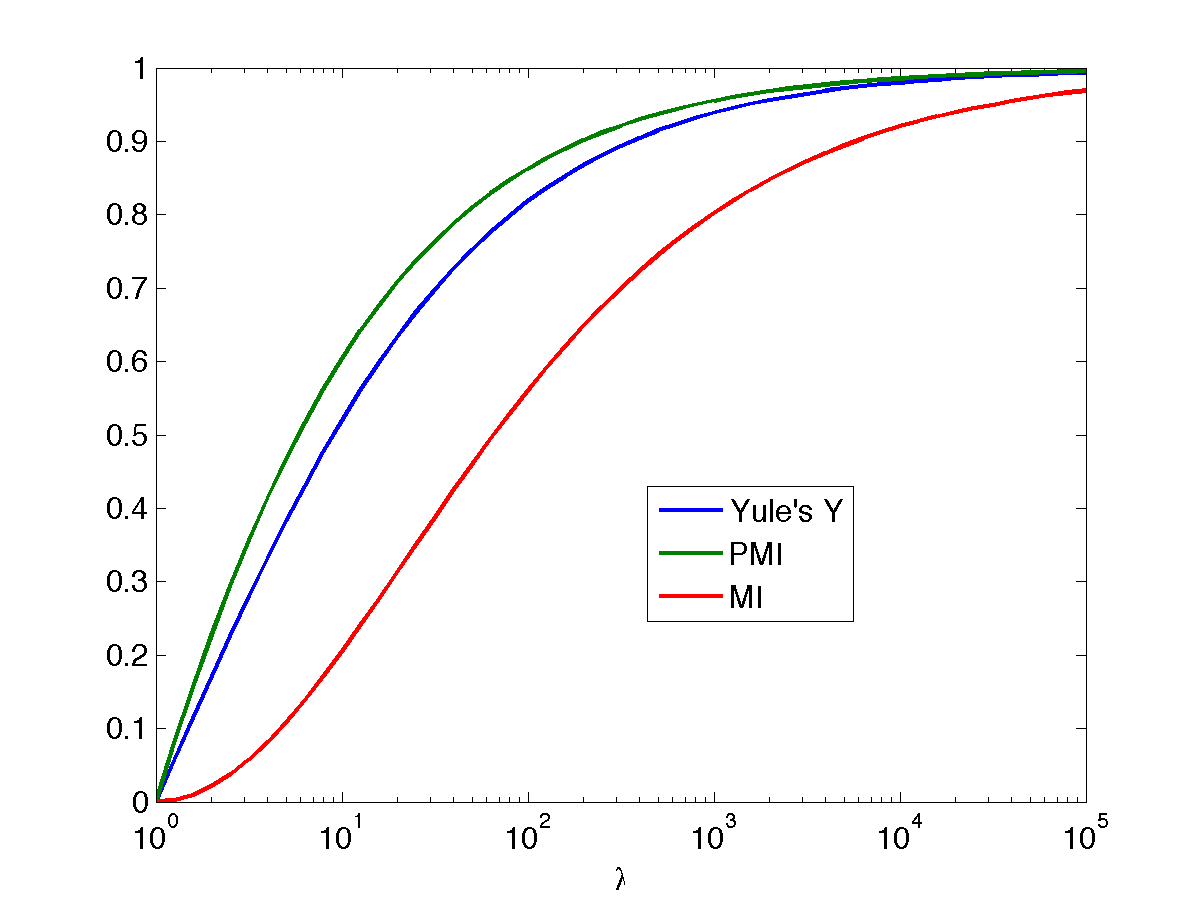
Figure 1: Plots of $Y$, $i_{\lambda}$ (PMI) and $I_{\lambda}$ (MI) against $\lambda$ (log scale) for $\lambda\geq 1$.

Plots of $Y$, $i_{\lambda}$ and $I_{\lambda}$ for $\lambda\geq 1$ in Figure 1 show a similar behaviour, monotonically increasing to a maximum value as $\lambda\rightarrow\infty$. If we choose logs to base 2, then the maximum value is 1 in all three cases. As $Y$ is already well-established (since 1912!), it does not seem necessary to promote $i_{\lambda}$ or $I_{\lambda}$ as alternatives, when considering the canonical table.

recover die marginals vaccinated 0.840 0.043 0.883 unvaccinated 0.059 0.058 0.117 marginals 0.899 0.101	0.476 0.024 0.500 0.252 0.248 0.500 0.728 0.272	0.408 0.092 0.500 0.092 0.408 0.500 0.500 0.500
PMI = 2.300, MI = 0.108	PMI = 0.866, MI = 0.205	PMI = 0.705, MI = 0.310
(a) original table	(b) vaccination rate 50%	(c) canonical table

Table 1: $2\times 2$ contingency tables for the association between vaccination and death from smallpox. (a) is the original table based on the data in Yule, (1912), (b) adjusts the marginals for vaccinated/unvaccinated to be 50/50, and (c) is the canonical table where the marginals are both 50/50. In all three tables, Yule’s $Y=0.630$.

Detecting Associations with Pointwise Mutual Information

As we have seen, the raw PMI score is not invariant to the distribution of the marginals. This can be seen in Table 1, which concerns the association between vaccination and death from smallpox; the original proportions in panel (a) are based on the Sheffield data in Table I of Yule, (1912). In panel (b) the marginals of the table wrt vaccination have been adjusted to 50/50 (as may have happened if these data had been collected in a randomized controlled trial), and in panel (c) we have the canonical table where both marginals are 50/50. Notice that the PMI is highest for the original (unbalanced) table, and decreases as the marginals are balanced. Conversely the MI is lowest in the the original (unbalanced) table, and increases as the marginals are balanced. Of course Yule’s $Y$ is constant throughout, by construction.

As another example, consider fixing $\lambda$ but adjusting the marginal probabilities of events $x$ and $y$. For example, for $\lambda=16$, PMI takes on the values of 0.678, 1.642, 2.293, 3.642 and 3.958 (using logs to base 2) as $p(x)=p(y)$ varies from 0.5, 0.2, 0.1, 0.01 and 0.001. This is particularly problematic as low counts will give rise to uncertainty in the estimation of the required probabilities (especially of the joint event). In the context of word associations, Manning and Schütze, (1999, sec. 5.4) argue that PMI “does not capture the intuitive notion of an interesting collocation very well”, and mention work which multiplies it by $p(x,y)$ as one strategy to compensate for the bias in favour of rare events.

On the other hand, Barlow, (1985) suggested that sparsity is important for the detection of suspicious coincidences, i.e. that “the events themselves must be rare ones”. It is true that a low $p(y)$ gives more “headroom” for the ratio $p(y|x)/p(y)$ to be large. The PMI score is used extensively in pharmacovigilance, where the aim is to detect associations between drugs taken and adverse drug reactions (ADRs). In this context, the ratio $p(x,y)/p(x)p(y)=p(y|x)/p(y)$ is termed the relative reporting ratio (RRR), and compares the relative probability of an adverse drug reaction $y$ given treatment with drug $x$, compared to the base rate $p(y)$. Another commonly used measure is the proportional reporting ratio (PRR), defined as $p(y|x)/p(y|\neg x)$. The US Food and Drug Administration (FDA) white paper (Duggirala et al.,, 2018) describes the use of both RRR and PRR for detecting ADRs in routine surveillance activities.

Above we have described maximum likelihood estimation for the probabilities in the $2\times 2$ table, based on counts. However, there are well-known issues with the MLE when (some of) the counts are small. This naturally suggests a Bayesian approach, and there is a considerable literature on the Bayesian analysis of contingency tables, as reviewed e.g. in Agresti, (2013). There are different sampling models depending on how the data is assumed to be generated, as described in Agresti, (2013, sec. 2.1.5). If all 4 counts are unrestricted, a natural assumption is that each $n_{ij}$ is drawn from a Poisson distribution with mean $\mu_{ij}$, which can be given a Gamma prior. Alternatively if $n$ is fixed, the sampling model is a multinomial, and the conjugate prior is a Dirichlet distribution. If one set of marginals is fixed, then the data is drawn from two Binomial distributions, each of which can be given a Beta prior. If both marginal totals are fixed, this corresponds to Fisher’s famous “Lady Tasting Tea” experiment, and the sampling distribution of any cell in the table follows a hypergeometric distribution. Section 3.6 of Agresti, (2013) covers Bayesian inference for two-way contingency tables, and Agresti and Min, (2005) discuss Bayesian confidence intervals for association parameters, such as the odds ratio.

DuMouchel, (1999) applied an Empirical Bayes approach to consider sampling variability for PMI (aka RRR) in the context of adverse drug reactions. He assumed that each $n_{11}$ is a draw from a Poisson distribution with unknown mean $\mu_{11}$, and that the object of interest is $\rho_{11}=\mu_{11}/E_{11}$, where $E_{11}$ is the expected count (assumed known) under the assumption that the variables are independent. Using a mixture of Gamma distributions prior for $\rho_{11}$, DuMouchel obtained the posterior mean $E[\log(\rho_{11})|n_{11}]$, rather than just considering the sample estimate $n_{11}/E_{11}$. The mixture prior was used to express the belief that when testing many associations, most will have a PMI of near 0, but there will be some that have significantly larger values. This method is known as the Multi-Item Gamma Poisson Shrinker (MGPS). The value of this approach is that Bayesian shrinkage corrects for the high variability in the RRR sample estimate $n_{11}/E_{11}$ that results from small counts.

Summary

Motivated by Barlow’s hypothesis about suspicious coincidences, we have reviewed the properties of $2\times 2$ contingency tables for association analysis, with a focus on the odds ratio $\lambda$ and Yule’s $Y$. We have considered the mutual information and pointwise mutual information as measures of association, along with normalized versions thereof. We have shown that, considered as functions of $\lambda$ in the canonical table, MI and PMI behave similarly to $Y$ for $\lambda\geq 1$, increasing monotonically with $\lambda$ (and can be made similar for $0<\lambda<1$).

As well as $Y$, the PMI measure $i(x,y)=\log p(x,y)/(p(x)p(y)$ can also be used to identify suspicious coincidences, and it is used in practice, for example, in pharmacovigilance. We have discussed the pros and cons of using it in this way, bearing in mind the sensitivity of the PMI to the marginals, with increased scores for sparser events. When some of the counts in the table are low, Bayesian approaches can be useful for the estimation of PMI from raw counts.

Addendum: Earlier Work on Pointwise Mutual Information

Subsequent to the publication of this paper, I became aware of the paper by Good, (1956), which terms pointwise mutual information the “association factor”. In this paper on p. 114 Good mentions a number of earlier references to this quantity. I have been able to trace discussion of PMI to Woodward, (1953, p. 53) (where it is termed the “information transfer between x and y”), and (without the log) to Keynes, (1921, p. 170) (where it is termed the “coefficient of dependence”). For the latter reference, the paper by Brössel, (2015) was helpful in tracking down the citation.

References

- Agresti, (2013) Agresti, A. (2013). Categorical Data Analysis. John Wiley and Sons, Third edition.
- Agresti and Min, (2005) Agresti, A. and Min, Y. (2005). Frequentist Performance of Bayesian Confidence Intervals for Comparing Proportions in Contingency Tables. Biometrics, 61:515–523.
- Barlow, (1985) Barlow, H. B. (1985). Cerebral cortex as model builder. In Rose, D. and Dobson, V. G., editors, Models of the Visual Cortex, page 37–46. John Wiley & Sons Ltd.
- Barlow, (1987) Barlow, H. B. (1987). Cerebral Cortex as Model Builder. In Vaina, L. M., editor, Matters of Intelligence: conceptual structures in cognitive neuroscience , pages 395–406. D. Reidel Publishing Company.
- Bate et al., (1998) Bate, A. et al. (1998). A Bayesian neural network method for adverse drug reaction signal detection. European Journal of Clinical Pharmacology, 54:315–321.
- Bouma, (2009) Bouma, G. (2009). Normalized (Pointwise) Mutual Information in Collocation Extraction. In Proceedings of the Biennial GSCL Conference 2009.
- Brössel, (2015) Brössel P. (2015). Keynes’s Coefficient of Dependence Revisited. Erkenntnis, 80:521–553.
- Church and Hanks, (1990) Church, K. W. and Hanks, P. (1990). Word association norms, mutual information, and lexicography. Comput. Linguist., 16(1):22–29.
- Duggirala et al., (2018) Duggirala, H. J. et al. (2018). Data Mining at FDA—White Paper. Available from https://www.fda.gov/science-research/data-mining/data-mining-fda-white-paper. Content is specified as current as of 08/20/2018.
- DuMouchel, (1999) DuMouchel, W. (1999). Bayesian Data Mining in Large Frequency Tables, with an Application to the FDA Spontaneous Reporting System. American Statistician, 53(3):177–190.
- Edelman et al., (2002) Edelman, S., Hiles, B., Yang, H., and Intrator, N. (2002). Probabilistic principles in unsupervised learning of visual structure: human data and a model. In Dietterich, T., Becker, S., and Ghahramani, Z., editors, Advances in Neural Information Processing Systems, volume 14. MIT Press.
- Edwards, (1963) Edwards, A. W. F. (1963). The Measure of Association in a Table. Journal of the Royal Statistical Society. Series A (General), 126(1):109–114.
- Good, (1956) Good, I. J. (1956). On the Estimation of Small Frequencies in Contingency Tables. Journal of the Royal Statistical Society. Series B (Methodological), 18(1):113–124.
- Hasenclever and Scholz, (2016) Hasenclever, D. and Scholz, M. (2016). Comparing Measures of Association in Probability Tables. The Open Statistics & Probability Journal, 7:20–35.
- Keynes, (1921) Keynes, J. M. (1921). A Treatise on Probability. London, Macmillan.
- Lewontin, (1964) Lewontin, R. C. (1964). The Interaction of Selection and Linkage. I. General Considerations; Heterotic Models. Genetics, 49(1):49–67.
- Manning and Schütze, (1999) Manning, C. and Schütze, H. (1999). Foundations of Statistical Natural Language Processing. MIT Press.
- Press et al., (2007) Press, W. H., Teukolsky, S. A., Vetterling, W. T., and Flannery, B. P. (2007). Numerical Recipes: The Art of Scientific Computing. Cambridge University Press, Third edition.
- Silverstein et al., (1998) Silverstein, C., Brin, S., and Motwani, R. (1998). Beyond Market Baskets: Generalizing Association Rules to Dependence Rules. Data Mining and Knowledge Discovery, 2(1):39–68.
- Tan et al., (2004) Tan, P.-N., Kumar, V., and Srivastva, J. (2004). Selecting the right objective measure for association analysis. Information Systems, 29:293–313.
- Woodward, (1953) Woodward, P. M.. (1953). Probability and Information Theory, with Applications to Radar. London, Pergamon Press.
- Yule, (1912) Yule, G. U. (1912). On the Methods of Measuring Association Between Two Attributes. Journal of the Royal Statistical Society, 75(6):579–652.