Interacting electrons and bosons in the doubly screened $G\widetilde{W}$ approximation: A time-linear scaling method for first-principles simulations

Abstract

We augment the time-linear formulation of the Kadanoff-Baym equations for systems of interacting electrons and quantized phonons or photons with the $G\widetilde{W}$ approximation, the Coulomb interaction $\widetilde{W}$ being dynamically screened by both electron-hole pairs and bosonic particles. We also show how to combine different approximations to include simultaneously multiple correlation effects in the dynamics. The final outcome is a versatile framework comprising $2^{12}$ distinct diagrammatic methods, each scaling linearly in time and preserving all fundamental conservation laws. The dramatic improvement over current state-of-the-art approximations brought about by $G\widetilde{W}$ is demonstrated in a study of the correlation-induced charge migration of the glycine molecule in an optical cavity.

Introduction: After Feynman’s visionary idea in 1949 [1] the Green’s function (GF) diagrammatic theory has developed into a powerful and versatile approach in nearly every field of theoretical physics. In condensed matter theory [2, 3, 4, 5] efforts toward the nonequilibrium extension of the formalism (NEGF) [6, 7] culminated in the so-called Kadanoff-Baym equations (KBE) [8, 9]. The KBE govern the dynamics of correlated electrons and bosons and give access to the electronic, magnetic and optical properties of any quantum system, from simple molecules to bulk materials. As for any exact reformulation of the many-body Schrödinger equation the applicability of the KBE relies on accurate approximations and efficient implementation schemes [10, 11, 12, 13].

In Ref. [14] we built on the Generalized Kadanoff-Baym Ansatz (GKBA) for electrons [15] and bosons [16] and on the time-linear formulation of the GKBA-KBE with electron-electron ($e$-$e$) [17, 18] and electron-boson ($e$-$b$) [16] interactions to map a broad class of NEGF approximations onto a coupled system of ordinary differential equations (ODE). Available methods to treat $e$-$e$ correlations include $GW$ [19], $T$-matrix (either without or with exchange) and Faddeev [20] while $e$-$b$ correlations are described by Ehrenfest and second-order diagrams in the $e$-$b$ coupling [21, 22, 23, 24]. Every method in this NEGF toolbox guarantees the fulfillment of all fundamental conservation laws [25, 26, 9].

In this work we present a substantial advance in the treatment of correlations, requiring no extra computational cost and preserving all conserving properties. Specifically we include the effects of dynamical screening due to both $e$-$e$ and $e$-$b$ interactions ($G\widetilde{W}$ approximation) [27, 28]. The $G\widetilde{W}$ extention opens the door to a wealth of phenomena ranging from carrier relaxation [29, 30] and exciton recombination [31, 32] to molecular charge migration and transfer in optical or plasmonic cavities [33, 34, 35, 36]. We further show how to combine different methods without incurring any double counting. The final outcome is a NEGF toolbox that can be used to investigate the correlated dynamics of electrons and bosons in $2^{12}$ distinct diagrammatic approximations. Real-time simulations of the correlation-induced charge migration of the glycine molecule in an optical (or plasmonic) cavity demonstrates the superiority of the $G\widetilde{W}$ method over other approximations.

Preliminaries: We consider a system of electrons with one-particle time-dependent Hamiltonian $h_{ij}(t)$ and $e$-$e$ interaction $v_{ijmn}$ (Latin indices $i,j,\ldots$ etc. specify the spin-orbitals of an orthonormal basis) coupled linearly to the displacement $\hat{\phi}_{\mbox{\scalebox{0.7}{$\scriptscriptstyle\mbox{\boldmath$\mu$}$}},1}\equiv\hat{x}_{\mbox{\scalebox{0.7}{$\scriptscriptstyle\mbox{\boldmath$\mu$}$}}}=(\hat{a}^{{\dagger}}_{\mbox{\scalebox{0.7}{$\scriptscriptstyle\mbox{\boldmath$\mu$}$}}}+\hat{a}_{\mbox{\scalebox{0.7}{$\scriptscriptstyle\mbox{\boldmath$\mu$}$}}})/\sqrt{2}$ and momentum $\hat{\phi}_{\mbox{\scalebox{0.7}{$\scriptscriptstyle\mbox{\boldmath$\mu$}$}},2}=\hat{p}_{\mbox{\scalebox{0.7}{$\scriptscriptstyle\mbox{\boldmath$\mu$}$}}}=i(\hat{a}^{{\dagger}}_{\mbox{\scalebox{0.7}{$\scriptscriptstyle\mbox{\boldmath$\mu$}$}}}-\hat{a}_{\mbox{\scalebox{0.7}{$\scriptscriptstyle\mbox{\boldmath$\mu$}$}}})/\sqrt{2}$ of a set of bosonic modes of frequency $\omega_{\mbox{\scalebox{0.7}{$\scriptscriptstyle\mbox{\boldmath$\mu$}$}}}$. Introducing the Greek index $\mu=(\mbox{\boldmath$\mu$},\xi)$ with $\xi=1,2$, we denote by $g_{\mu,ij}$ the interaction strength of the $e$-$b$ coupling. The equation of motion (EOM) for the one-electron density matrix $\rho^{<}_{ij}(t)\equiv\langle\hat{d}_{j}^{\dagger}(t)\hat{d}_{i}(t)\rangle$ [with $\hat{d}^{({\dagger})}$’s the electronic annihilation (creation) operators] and one-boson density matrix $\gamma_{\mu\nu}^{<}(t)\equiv\langle\Delta\hat{\phi}_{\nu}(t)\Delta\hat{\phi}_{\mu}(t)\rangle$ [with $\Delta\hat{\phi}_{\nu}\equiv\hat{\phi}_{\nu}-\langle\hat{\phi}_{\nu}\rangle$ the bosonic fluctuation operator] reads [16]

$$i\frac{d}{dt}\rho^{<}(t) =\big{[}h^{e}(t),\rho^{<}(t)\big{]}-i\left(I^{e}(t)+I^{e\,\dagger}(t)\right),$$ (1a)

$$i\frac{d}{dt}\mbox{\boldmath$\gamma$}^{<}(t)$$

where $h^{e}_{ij}(t)=h_{ij}(t)+\sum_{mn}[v_{imnj}(t)-v_{imjn}(t)]\rho^{<}_{nm}(t)+\sum_{\mu}g_{\mu,ij}(t)\phi_{\mu}(t)$ is the mean-field electronic Hamiltonian [$\phi_{\mu}=\langle\hat{\phi}_{\mu}\rangle$ for brevity] whereas $\mathbfit{h}^{b}(t)=2\mbox{\boldmath$\alpha$}\bm{\Omega}(t)$, with $\alpha_{\mu\mu^{\prime}}\equiv\delta_{\mbox{\scalebox{0.7}{$\scriptscriptstyle\mbox{\boldmath$\mu$}$}}\mbox{\scalebox{0.7}{$\scriptscriptstyle\mbox{\boldmath$\mu$}$}}^{\prime}}\begin{pmatrix}0&i\\ -i&0\end{pmatrix}_{\xi\xi^{\prime}}$ and $\Omega_{\mu\mu^{\prime}}(t)\equiv\frac{1}{2}\delta_{\mu\nu}\omega_{\mbox{\scalebox{0.7}{$\scriptscriptstyle\mbox{\boldmath$\mu$}$}}}(t)$, is the free-boson Hamiltonian. To distinguish matrices in the one-electron space from matrices in the one-boson space we use boldface for the latters. The time-dependence of the $e$-$e$ coupling $v_{ijmn}(t)$ and $e$-$b$ coupling $g_{\mu,ij}(t)$ could be due to the adiabatic switching protocol adopted to generate a correlated initial state [37], whereas the time-dependence of the one-particle Hamiltonian $h_{ij}(t)$ and bosonic frequencies $\omega_{\mbox{\scalebox{0.7}{$\scriptscriptstyle\mbox{\boldmath$\mu$}$}}}(t)$ could be due to some external field, e.g., laser fields [38, 39], phonon drivings [40], etc. As the mean-field Hamiltonian $h^{e}$ depends on $\phi_{\mu}(t)$ the EOM (1) must be complemented with the Ehrenfest EOM for the displacements and momenta of the bosonic modes, see below.

The collision integrals $I^{e}$ and $\mathbfit{I}^{b}$ accounts for all effects beyond mean-field. They can be written in terms of two high-order GFs according to [16] $I^{e}_{lj}=i\sum_{\mu,i}g_{\mu,li}\mathcal{G}^{b}_{\mu,ij}-i\sum_{imn}v_{lnmi}\mathcal{G}^{e}_{imjn}$ and $I^{b}_{\mu\nu}=-i\sum_{\nu,mn}\alpha_{\mu\nu}g_{\nu,mn}\mathcal{G}^{b}_{\nu,nm}$, where

$$\mathcal{G}^{e}_{imjn}(t) =-\langle\hat{d}^{{\dagger}}_{n}(t)\hat{d}^{{\dagger}}_{j}(t)\hat{d}_{i}(t)\hat{d}_{m}(t)\rangle_{c},$$ (1b)

$$\mathcal{G}^{b}_{\mu,ij}(t) =\langle\hat{d}^{{\dagger}}_{j}(t)\hat{d}_{i}(t)\hat{\phi}_{\mu}(t)\rangle_{c}.$$ (1c)

The subscript “$c$” in the averages signifies that only the correlated part must be retained. The EOM (1) fulfill all fundamental conservation laws if $\mathcal{G}^{e}$ and $\mathcal{G}^{b}$ are obtained from the functional derivatives of the correlated part $\Phi_{c}$ of the Baym functional [26] with respect to the $e$-$e$ and $e$-$b$ coupling respectively, i.e.,

$$\mathcal{G}^{e}_{imjn}(t) =i\frac{\delta\Phi_{c}}{\delta v_{jnmi}(t)}+i\frac{\delta\Phi_{c}}{\delta v_{njim}(t)},$$ (1da)

$$\mathcal{G}^{b}_{\mu,ij}(t) =\frac{1}{i}\,\frac{\delta\Phi_{c}}{\delta g_{\mu,ji}(t)}.$$ (1db)

In Ref. [16] we have considered the correlated functional $\Phi_{c}=$ – full lines represent electronic GFs $G$, zig-zag lines bosonic GFs $D$ and empty circles the $e$-$b$ coupling $g$. The mathematical expression of the considered functional reads (time integrals are over the Keldysh contour)

$$\Phi_{c}=-\frac{1}{2}\int\!d\bar{t}d\bar{t}^{\prime}\,{\rm Tr}[\mbox{\boldmath$g$}^{{\dagger}}(\bar{t})\mathbfit{D}(\bar{t},\bar{t}^{\prime})\mbox{\boldmath$g$}(\bar{t}^{\prime})\bm{\mathit{\chi}}^{0}(\bar{t}^{\prime},\bar{t})],$$ (1e)

where we have defined the matrix $g$ with elements $g_{\mu\nu}=g_{\mu,\begin{subarray}{c}j\\ i\end{subarray}}=g_{\mu,ij}$ (hence the second Greek-index $\nu=\bigl{(}\begin{smallmatrix}j\\ i\end{smallmatrix}\bigr{)}$ labels a pair of electronic indices) and the electronic response function $\chi^{0}_{\mu\nu}(t^{\prime},t)=\chi^{0}_{\begin{subarray}{c}qj\\ si\end{subarray}}(t^{\prime},t)\equiv-iG_{qj}(t^{\prime},t)G_{is}(t,t^{\prime})$. Consistently with our notation, matrices with Greek indices are represented by boldface letters. Through Eqs. (1d) one obtains $\mathcal{G}^{e}=0$ and $\bm{\mathcal{G}}^{b}(t)=i\int d\bar{t}\mathbfit{D}(t,\bar{t})\mbox{\boldmath$g$}(\bar{t})\bm{\mathit{\chi}}^{0}(\bar{t},t^{+})$. Implementing the GKBA for electrons and bosons [15, 16],

$$G^{\lessgtr}(t,t^{\prime} =-G^{R}(t,t^{\prime})\rho^{\lessgtr}(t^{\prime})+\rho^{\lessgtr}(t)G^{A}(t,t^{\prime}),$$ (1f)

$$\mathbfit{D}^{\lessgtr}(t,t^{\prime}) =\mathbfit{D}^{R}(t,t^{\prime})\mbox{\boldmath$\alpha$}\mbox{\boldmath$\gamma$}^{\lessgtr}(t^{\prime})-\mbox{\boldmath$\gamma$}^{\lessgtr}(t)\mbox{\boldmath$\alpha$}\mathbfit{D}^{A}(t,t^{\prime}),$$ (1g)

one can show that $\bm{\mathcal{G}}^{b}$ satisfies a first-order ODE [16] whose coefficients are given by simple functionals of the density matrices $\rho^{<}$, $\rho^{>}\equiv\rho^{<}-1$ and $\mbox{\boldmath$\gamma$}^{<}$, $\mbox{\boldmath$\gamma$}^{>}\equiv\mbox{\boldmath$\gamma$}^{<}+\mbox{\boldmath$\alpha$}$. This is pivotal for constructing a time-linear scheme. The resulting GKBA+ODE are equivalent to the original KBE — in the GKBA framework — with electronic self-energy in the $GD$ approximation [41, 42, 23] and bosonic self-energy proportional to $\bm{\mathit{\chi}}^{0}$. The feedback of electrons (bosons) on the bosonic (electronic) subsystem underlies the fulfillment of all conservation laws.

The doubly screened $G\widetilde{W}$ method: The functional $\Phi_{c}$ in Eq. (1e) is independent of the $e$-$e$ interaction; hence electronic screening of the $e$-$b$ coupling is not accounted for. This is a severe drawback for extended systems [43, 44]. State-of-the-art calculations of electronic life-times [45], polaron dispersions [46] and carrier dynamics [30] are indeed performed with a statically screened electron-phonon coupling [47, 48, 49]. Formally, static screening does not involve any generalization of the $GD$ equations: it is sufficient to replace one of the $g$’s in Eq. (1e) with $\mbox{\boldmath$g$}^{s}=\mbox{\boldmath$g$}(1+\bm{\mathit{\chi}}^{s}\mathbfit{v})$, where $v_{\begin{subarray}{c}im\\ nj\end{subarray}}\equiv v_{ijmn}$ and $\bm{\mathit{\chi}}^{s}$ is the random phase approximation (RPA) response function, $\bm{\mathit{\chi}}=\bm{\mathit{\chi}}^{0}+\bm{\mathit{\chi}}\mathbfit{v}\bm{\mathit{\chi}}^{0}$, evaluated in equilibrium and at zero frequency. Although $\mbox{\boldmath$g$}^{s}$ is an improvement over the bare $g$, retardation effects and nonequilibrium corrections are still lacking. In the following we show that a time-linear GKBA+ODE scheme can be formulated for the two-times dynamically screened coupling $\mbox{\boldmath$g$}^{d}=\mbox{\boldmath$g$}(1+\bm{\mathit{\chi}}\mathbfit{v})$.

It is fundamental to observe that the GKBA GFs in Eqs. (1f,1g) are mean-field like GFs. The theory can therefore be improved in a conserving fashion by calculating $\mathcal{G}^{e}$ and $\mathcal{G}^{b}$ from the reducible Baym functional $\Phi_{c}^{(r)}$ [9]. Let $\Phi_{c}^{(r)}$ be the $G\widetilde{W}$ functional in Fig. 1(a) where $\widetilde{\mathbfit{v}}=\mathbfit{v}+\mbox{\boldmath$g$}^{{\dagger}}\mathbfit{D}\mbox{\boldmath$g$}$. This functional is reducible with respect to $\mathbfit{D}$ but no double counting occurs if $\mathbfit{D}$ is evaluated from Eq. (1g). Remarkably, a time-linear GKBA+ODE scheme can be formulated in this case too. The zeroth order contribution (in $g$) is the well known $GW$ approximation while the second-order contribution corresponds to the aforementioned approximation with dynamically screened $\mbox{\boldmath$g$}^{d}$, henceforth $G\widetilde{W}^{(2)}$.

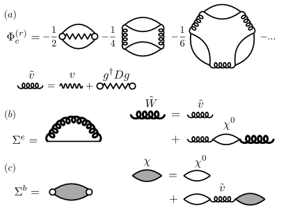
Figure 1: (a) Diagrams of the reducuble $G\widetilde{W}$ functional $\Phi_{c}^{(r)}$. Full lines are used for $G$, zig-zag lines are used for $D$, empty circles are used for $g$, wavy lines are used for $v$ and gluon lines are used for $\widetilde{v}$. (b) Electronic self-energy in terms of the doubly screened interaction $\widetilde{W}$. (c) Bosonic self-energy in terms of the doubly screened response function $\chi$.

The high-order GFs of the doubly screened $G\widetilde{W}$ scheme follow from Eqs. (1d) with $\Phi_{c}^{(r)}$ in place of $\Phi_{c}$ (time integrals are over the Keldysh contour)

$$\bm{\mathcal{G}}^{e}(t) =-i\int d\bar{t}d\bar{t}^{\prime}\bm{\mathit{\chi}}(t,\bar{t})\widetilde{\mathbfit{v}}(\bar{t},\bar{t}^{\prime})\bm{\mathit{\chi}}^{0}(\bar{t}^{\prime},t^{+}),$$ (1ha)

$$\bm{\mathcal{G}}^{b}(t) =i\int d\bar{t}\mathbfit{D}(t,\bar{t})\mbox{\boldmath$g$}(\bar{t})\bm{\mathit{\chi}}(\bar{t},t^{+}).$$ (1hb)

In analogy with $\bm{\mathit{\chi}}$ and $\mathbfit{v}$ we have defined $\bm{\mathcal{G}}^{e}$ as a matrix in the two-electron space with elements $\mathcal{G}^{e}_{\mu\nu}=\mathcal{G}^{e}_{\begin{subarray}{c}mj\\ ni\end{subarray}}=\mathcal{G}^{e}_{imjn}$, and in analogy with $g$ we have defined $\bm{\mathcal{G}}^{b}$ as a matrix with elements $\mathcal{G}^{b}_{\mu\nu}=\mathcal{G}^{b}_{\mu,\begin{subarray}{c}j\\ i\end{subarray}}=\mathcal{G}^{b}_{\mu,ij}$. The solution of the EOM (1) with $\bm{\mathcal{G}}^{e}$ and $\bm{\mathcal{G}}^{b}$ from Eqs. (1h) is equivalent to solving the KBE with electronic (nonskeletonic) self-energy $\Sigma^{e}=-iG\widetilde{W}$, see Fig. 1(b), and bosonic (reducible) self-energy $\mathbfit{\Sigma}^{b}=\mbox{\boldmath$g$}\bm{\mathit{\chi}}\mbox{\boldmath$g$}^{\dagger}$, see Fig. 1(c). The nonskeletonicity and reducibility is equivalent to dressing of the GKBA $\mathbfit{D}$.

The GKBA in Eqs. (1f,1g) can be used to transform $\bm{\mathcal{G}}^{e}$ and $\bm{\mathcal{G}}^{b}$ into functionals of $\rho^{<}$ and $\mbox{\boldmath$\gamma$}^{<}$, see Appendix A, thus closing the EOM for these quantities. Interestingly, however, the EOM for these high-order GFs form a closed system. We separate the two-particle GF into a purely electronic part $\bm{\mathcal{G}}^{ee}\equiv\bm{\mathcal{G}}^{e}|_{g=0}$ (diagrams with no $e$-$b$ vertices) and a rest $\bm{\mathcal{G}}^{eb}$, hence $\bm{\mathcal{G}}^{e}=\bm{\mathcal{G}}^{ee}+\bm{\mathcal{G}}^{eb}$, and show in Appendix B that (omitting the dependence on the time variable)

$$i\frac{d}{dt}\bm{\mathcal{G}}^{ee} =-\bm{\Psi}^{e}+\mathbfit{h}^{e}_{\rm eff}\bm{\mathcal{G}}^{ee}-\bm{\mathcal{G}}^{ee}\mathbfit{h}^{e\dagger}_{\rm eff},$$ (1ia)

$$i\frac{d}{dt}\bm{\mathcal{G}}^{eb} =\bm{\rho}^{\Delta}\mbox{\boldmath$g$}^{\dagger}\bm{\mathcal{G}}^{b}-\bm{\mathcal{G}}^{b\dagger}\mbox{\boldmath$g$}\bm{\rho}^{\Delta}+\mathbfit{h}^{e}_{\rm eff}\bm{\mathcal{G}}^{eb}-\bm{\mathcal{G}}^{eb}\mathbfit{h}^{e\dagger}_{\rm eff},$$ (1ib)

$$i\frac{d}{dt}\bm{\mathcal{G}}^{b} =-\bm{\Psi}^{b}-\mbox{\boldmath$\alpha$}\mbox{\boldmath$g$}\bm{\mathcal{G}}^{e}-\bm{\mathcal{A}}\mbox{\boldmath$g$}\bm{\rho}^{\Delta}+\mathbfit{h}^{b}\bm{\mathcal{G}}^{b}-\bm{\mathcal{G}}^{b}\mathbfit{h}^{e\dagger}_{\rm eff},$$ (1ic)

$$i\frac{d}{dt}\bm{\mathcal{A}} =\bm{\mathcal{G}}^{b}\mbox{\boldmath$g$}^{\dagger}\mbox{\boldmath$\alpha$}-\mbox{\boldmath$\alpha$}\mbox{\boldmath$g$}\bm{\mathcal{G}}^{b\dagger}+\mathbfit{h}^{b}\bm{\mathcal{A}}-\bm{\mathcal{A}}\mathbfit{h}^{b},$$ (1id)

where $\bm{\mathcal{A}}$ is an auxiliary quantity needed to close the EOM. The driving terms $\bm{\Psi}^{e}$ and $\bm{\Psi}^{b}$ are functionals of $\rho^{<}$ and $\mbox{\boldmath$\gamma$}^{<}$. They have been already encountered in Refs. [17, 16] in the context of the simpler $GW$ and $GD$ approximations. In particular

$$\bm{\Psi}^{e}(t) \equiv\bm{\rho}^{>}(t)\mathbfit{v}(t)\bm{\rho}^{<}(t)-\bm{\rho}^{<}(t)\mathbfit{v}(t)\bm{\rho}^{>}(t).$$ (1j)

$$\bm{\Psi}^{b}(t) \equiv\mbox{\boldmath$\gamma$}^{>}(t)\mbox{\boldmath$g$}(t)\bm{\rho}^{<}(t)-\mbox{\boldmath$\gamma$}^{<}(t)\mbox{\boldmath$g$}(t)\bm{\rho}^{>}(t),$$ (1k)

and $\mathbfit{h}^{e}_{\rm eff}=\mathbfit{h}^{e}-\bm{\rho}^{\Delta}\mathbfit{v}$ with $\bm{\rho}^{\Delta}=\bm{\rho}^{>}-\bm{\rho}^{<}$. The matrices $\mathbfit{h}^{e}$ and $\bm{\rho}^{\gtrless}$ in the two-electron space (hence represented by boldface letters) are defined with elements $h^{e}_{\mu\nu}=h^{e}_{\begin{subarray}{c}ij\\ mn\end{subarray}}=h^{e}_{ij}\delta_{nm}-\delta_{ij}h^{e}_{nm}$ and $\rho^{\lessgtr}_{\mu\nu}=\rho^{\lessgtr}_{\begin{subarray}{c}ij\\ mn\end{subarray}}=\rho^{\lessgtr}_{ij}\rho^{\gtrless}_{nm}$.

Equations (1,1i) together with the Ehrenfest equation for $\phi_{\mu}$, see below, form a system of seven first-order ODE that can be conveniently solved numerically using a time-stepping algorithm. This is the first main result of our work. The $G\widetilde{W}^{(2)}$ approximation is easily derived by discarding terms of order higher than $g^{2}$. In Appendix A we show that $\bm{\mathcal{G}}^{eb}={\mathcal{O}}(g^{2})$, $\bm{\mathcal{G}}^{b}={\mathcal{O}}(g)$ and $\bm{\mathcal{A}}={\mathcal{O}}(g^{2})$. Hence to second order in $g$ the r.h.s. of Eq. (1ic) can be calculated with $\mbox{\boldmath$g$}\bm{\mathcal{G}}^{e}\to\mbox{\boldmath$g$}\bm{\mathcal{G}}^{ee}$ and $\mbox{\boldmath$g$}\bm{\mathcal{A}}\to 0$; this implies that in $G\widetilde{W}^{(2)}$ the EOM for $\bm{\mathcal{A}}$ decouples. We also observe that the EOM in the $GD$ approximation, see Ref. [16], are recovered from the $G\widetilde{W}^{(2)}$ method upon setting $v=0$ (in this case we are left with only the equation for $\bm{\mathcal{G}}^{b}$). The EOM in the $GW$ approximation [17, 18, 20] are instead recovered from the full $G\widetilde{W}$ method upon setting $g=0$ (in this case we are left with only the equation for $\bm{\mathcal{G}}^{ee}$).

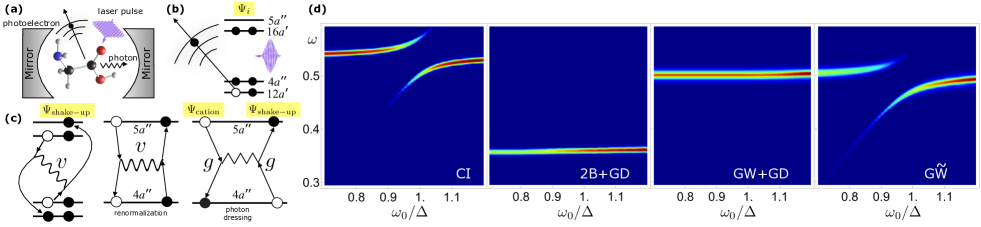
Figure 2: (a) Illustration of the gedanken experiment. A Gly molecule is ionized by a laser pulse and a cavity-photon is emitted. (b) The four MOs involved in the charge migration of Gly when the electron is ionized from the $12a^{\prime}$ MO. Electrons (black dots) on the MOs identify the state $\Psi_{i}$ after ionization. (c) Shake-up process leading to state $\Psi_{\rm shake-up}$ (left); scattering between electrons in the $4a^{\prime\prime}$ and $5a^{\prime\prime}$ MOs responsible for a sizable renormalization of the energy of the shake-up state (middle); electron-photon scattering leading to transition $\Psi_{\rm shake-up}\leftrightarrow\Psi_{\rm cation}$ (right). (d) Spectrograms of the occupancy of the $12a^{\prime}$ MO in different schemes.

Combining different methods: The treatment of pure electronic correlations is not limited to the $GW$ approximation. By properly modifying the index order of the matrices $\bm{\mathcal{G}}^{ee}$, $\bm{\rho}^{\lessgtr}$, $\mathbfit{h}^{e}$ and $\mathbfit{v}$ in Eq. (1ia) we can explore a large variety of methods [20]. They include the one-bubble or second-order direct (2B^d), second-order exchange (2B^x), $GW$, exchange-only $GW$ ($XGW$), $GW$ plus exchange ($GW+X$), $T$-matrix in the particle-hole channel ($T^{ph}$), exchange-only $T^{ph}$ ($XT^{ph}$), $T^{ph}$ plus exchange ($T^{ph}+X$), $T$-matrix in the particle-particle channel ($T^{pp}$) and exchange-only $T^{pp}$ ($XT^{pp}$), see Appendix C. Let “$c$” be the index for one of these correlated methods and let us denote by $\mathcal{G}^{ee(c)}_{imjn}$ the corresponding two-particle GF. Different methods can be combined to simultaneously include several types of correlation effects if the two-particle GF $\mathcal{G}^{ee}$ is evaluated according to

$$\mathcal{G}^{ee}_{imjn}(t)=\sum\nolimits_{c}n_{c}\mathcal{G}^{ee(c)}_{imjn}(t\,).$$ (1l)

In Appendix C we discuss how to choose the integers $n_{c}$ to avoid double countings. Decorating the electronic two-particle matrices $\bm{\rho}^{\lessgtr}$, $\mathbfit{h}^{e}$ and $\mathbfit{v}$ in the EOM for $\bm{\mathcal{G}}^{ee(c)}$ with the superscript $c$, the whole GKBA+ODE toolbox for interacting electrons and bosons can then be summarized as (omitting the dependence on the time variable)

$$i\frac{d}{dt}\phi_{\mu} =h^{b}_{\mu\nu}\phi_{\nu}+\sum\nolimits_{\nu,ij}\alpha_{\mu\nu}g_{\nu,ij}\rho_{ji},$$ (1ma)

$$i\frac{d}{dt}\rho^{<}_{lj} =\Bigl{\{}\sum_{i}h^{e}_{li}\rho^{<}_{ij}-\sum_{imn}v_{lnmi}\big{[}\mathcal{G}^{ee}_{imjn}+s_{1}d\mathcal{G}^{eb}_{imjn}\big{]}+d\sum_{\mu,i}g_{\mu,li}\,\mathcal{G}^{b}_{\mu,ij}\Bigr{\}}-\{l\leftrightarrow j\}^{\ast},$$ (1mb)

$$i\frac{d}{dt}\gamma_{\mu\nu}^{<} =\Bigl{\{}\sum_{\beta}h^{b}_{\mu\beta}\gamma^{<}_{\beta\nu}+d\sum_{\beta,mn}\alpha_{\mu\beta}g_{\beta,mn}\,\mathcal{G}^{b}_{\nu,nm}\Bigr{\}}-\{\mu\leftrightarrow\nu\}^{\ast},$$ (1mc)

$$i\frac{d}{dt}\bm{\mathcal{G}}^{ee(c)} =-\bm{\Psi}^{e(c)}+\mathbfit{h}^{e(c)}_{\rm eff}\bm{\mathcal{G}}^{ee(c)}-\bm{\mathcal{G}}^{ee(c)}\mathbfit{h}^{e(c)\dagger}_{\rm eff},$$ (1md)

$$i\frac{d}{dt}\bm{\mathcal{G}}^{eb} =\bm{\rho}^{\Delta(GW)}\mbox{\boldmath$g$}^{\dagger}\bm{\mathcal{G}}^{b}-\bm{\mathcal{G}}^{b\dagger}\mbox{\boldmath$g$}\bm{\rho}^{\Delta(GW)}+\mathbfit{h}^{e(GW)}_{\rm eff}\bm{\mathcal{G}}^{eb}-\bm{\mathcal{G}}^{eb}\mathbfit{h}^{e(GW)\dagger}_{\rm eff},$$ (1me)

$$i\frac{d}{dt}\bm{\mathcal{G}}^{b} =-\bm{\Psi}^{b}-s_{1}\mbox{\boldmath$\alpha$}\mbox{\boldmath$g$}\big{[}\bm{\mathcal{G}}^{ee(GW)}+s_{2}\bm{\mathcal{G}}^{eb}\big{]}-s_{1}s_{2}\bm{\mathcal{A}}\mbox{\boldmath$g$}\bm{\rho}^{\Delta(GW)}+\mathbfit{h}^{b}\bm{\mathcal{G}}^{b}-\bm{\mathcal{G}}^{b}\big{[}\mathbfit{h}^{e(GW)}-s_{1}\bm{\rho}^{\Delta(GW)}\mathbfit{v}^{(GW)}\big{]},$$ (1mf)

$$i\frac{d}{dt}\bm{\mathcal{A}} =\bm{\mathcal{G}}^{b}\mbox{\boldmath$g$}^{\dagger}\mbox{\boldmath$\alpha$}-\mbox{\boldmath$\alpha$}\mbox{\boldmath$g$}\bm{\mathcal{G}}^{b\dagger}+\mathbfit{h}^{b}\bm{\mathcal{A}}-\bm{\mathcal{A}}\mathbfit{h}^{b}.$$ (1mg)

The control parameters $d$, $s_{1}$ and $s_{2}$ refer to the treatment of $e$-$b$ correlations. The Ehrenfest approximation is recovered for $d=0$ – in this case the only equations to solve are those for the displacements and momenta, i.e., Eq. (1ma), and the electronic equations (1mb) and (1md). $e$-$b$ correlations are included choosing $d=1$. In this case we can set $(s_{1},s_{2})=(0,0)$ ($GD$), $(s_{1},s_{2})=(1,0)$ ($G\widetilde{W}^{(2)}$) and $(s_{1},s_{2})=(1,1)$ ($G\widetilde{W}$). The number of equations (1md) depends on the chosen treatment of electronic correlations, i.e., on the values of $n_{c}$’s. If $n_{c}=0$ the corresponding $\bm{\mathcal{G}}^{ee(c)}$ is not needed. The only exception is for $c=GW$: if $s_{1}=1$ then the EOM for $\bm{\mathcal{G}}^{ee(GW)}$ must be solved even for $n_{GW}=0$, see Eq. (1mf). The GKBA+ODE toolbox in Eqs. (1m) generalizes the one published in Ref. [14] in two ways (i) it includes the $G\widetilde{W}^{(2)}$ and $G\widetilde{W}$ methods and (2) it allows for combining different treatments of electronic correlations, for a total of $2^{12}$ distinct diagrammatic methods, see Appendix D. This is the second main result of our work.

Charge migration in a cavity: We consider the Gly I conformer of the glycine molecule and study the correlation-induced charge migration due to the removal of an electron from the 12$a^{\prime}$ molecular orbital (MO), see Fig. 2(b). In free space this case has been investigated at length [50, 51, 52, 53, 20]. Coulomb interaction is responsible for a shake-up process where an electron from the $16a^{\prime}$ MO fills the photo-hole and another electron is promoted from the $4a^{\prime\prime}$ MO to the initially empty $5a^{\prime\prime}$ MO, left of Fig. 2(c). We refer to our previous works for the electronic structure and basis representation [53, 54]. In Ref. [20] we showed that the energy of the shake-up state is strongly renormalized by the exchange interaction between electrons in the $4a^{\prime\prime}$ and $5a^{\prime\prime}$ MOs, middle of Fig. 2(c), and that capturing this renormalization requires a $GW$ treatment. Here we analyze how the dynamics is affected by a single cavity-mode that couples the shake-up state $\Psi_{\rm shake-up}$ to the lowest-energy cationic state $\Psi_{\rm cation}$ (one hole in $16a^{\prime}$ MO), right of Fig. 2(c).

Let $\Delta=E_{\rm shake-up}-E_{i}=0.522$ a.u. be the energy difference between $\Psi_{\rm shake-up}$ and the state $\Psi_{i}$ of Gly just after photo-ionization. In Fig. 2(d) we show the Fourier transform of the occupancy of the $12a^{\prime}$ MO for different frequencies $\omega_{0}$ of the cavity mode. The coupling $g=\lambda d_{4a^{\prime\prime},5a^{\prime\prime}}\sqrt{\omega_{0}}$ is proportional to the dipole moment $d_{4a^{\prime\prime},5a^{\prime\prime}}$ between the MOs involved in the transition $\Psi_{\rm shake-up}\to\Psi_{\rm cation}$. The electron-photon coupling strength $\lambda$ is determined by the mode wavefunction at the location of the molecule [55]. We take $d_{4a^{\prime\prime},5a^{\prime\prime}}=0.125$ a.u. as the average dipole moment along three orthogonal direction and choose $\lambda=0.212$ a.u.. Details on the numerical simulations can be found in Appendix E.

The first panel of Fig.2(d) displayes the Configuration Interaction (CI) spectrogram. For $\omega_{0}\ll\Delta$ cavity-photons are hardly emitted and the only possible transition is $\Psi_{i}\leftrightarrow\Psi_{\rm shake-up}$. Correspondingly, the spectrum has only one peak at frequency $\Delta_{\rm CI}=0.544~{}{\rm a.u.}~{}\simeq\Delta$. As $\omega_{0}$ approaches $\Delta$ an Autler-Townes doublet of entangled electron-photon many-body states becomes visible [56, 57]. It is due to the photon-dressing of the cationic state which makes the transition $\Psi_{i}\leftrightarrow\Psi_{\rm cation}$ bright and dominant when $\omega_{0}>\Delta$.

For a diagrammatic approximation to reproduce CI, the electronic self-energy must account for all three mechanisms illustrated in Fig. 2(c). In the second panel of Fig.2(d) we report the 2B+$GD$ spectrogram. This approximation captures only the shake-up process, thereby yielding a $\omega_{0}$-independent structure at energy $\Delta_{\rm 2B}=0.356$ a.u.. As expected [20], the $GW+GD$ method renormalizes $\Delta_{\rm 2B}$ to $\Delta_{GW}=0.503\simeq\Delta_{\rm 2B}+2v^{x}_{4a^{\prime\prime},5a^{\prime\prime}}$, see third panel, where $v^{x}_{4a^{\prime\prime},5a^{\prime\prime}}=0.08$ a.u. is the exchange Coulomb integral responsible for the scattering in Fig. 2(c) (middle). Achieving the CI value $\Delta$ calls for vertex corrections which, however, are beyond the current GKBA+ODE formulation. The most severe deficiency of the $GW+GD$ spectrogram is the absence of the Autler-Townes doublet. In fact, photon-dressing requires a non-perturbative treatment in the $e$-$b$ coupling like the $G\widetilde{W}$ method. The $G\widetilde{W}$ spectrogram is shown in the fourth panel. Although the intensity of the low-$\omega_{0}$ peak is weaker than in CI, the improvement over $GW+GD$ is quantitatively and qualitatively substantial.

In conclusion, we have extended the time-linear GKBA+ODE formulation for interacting fermions and bosons to the doubly screened $G\widetilde{W}$ method, and shown how to combine different diagrammatic approximations to account for multiple correlation effects simultaneously while preserving all conserving properties. The case of correlation-induced charge migration of glycine in an optical cavity exemplifies the superiority of $G\widetilde{W}$ over current state-of-the-art approaches. We emphasize that the scaling of a $G\widetilde{W}$ calculation with the system size is the same as for $GW$, thus making the method potentially available for real-time first-principles simulations of finite [54, 20] and extended [58, 19] systems. Last but not least the GKBA+ODE formulation lends itself to studies of multiscale phenomena through the implementation of adaptive time-stepping algorithms.

Appendix A GKBA form of $\mathcal{G}^{e}$ and $\mathcal{G}^{b}$

We here work out the GKBA expression for the high-order GFs in Eq. (1b) and (1c). Let us start from $\bm{\mathcal{G}}^{e}$. Using the Langreth rules we find

$$\bm{\mathcal{G}}^{e}(t) =\!\!\int\!\!d\bar{t}d\bar{t}^{\prime}\big{[}\bm{\mathit{\chi}}^{R}(t,\bar{t})\tilde{\mathbfit{v}}^{R}(\bar{t},\bar{t}^{\prime})\bm{\mathit{\chi}}^{0,<}(\bar{t}^{\prime},t)$$

$$+\!\bm{\mathit{\chi}}^{R}(t,\bar{t})\tilde{\mathbfit{v}}^{<}(\bar{t},\bar{t}^{\prime})\bm{\mathit{\chi}}^{0,A}(\bar{t}^{\prime},t)+\!\bm{\mathit{\chi}}^{<}(t,\bar{t})\tilde{\mathbfit{v}}^{A}(\bar{t},\bar{t}^{\prime})\bm{\mathit{\chi}}^{0,A}(\bar{t}^{\prime},t)\big{]},$$ (1n)

where all intergrals are now over the real axis. From the RPA equation $\bm{\mathit{\chi}}=\bm{\mathit{\chi}}^{0}+\bm{\mathit{\chi}}\tilde{\mathbfit{v}}\bm{\mathit{\chi}}^{0}$ (on the Keldysh contour) we can easily extract the retarded ($R$), advanced ($A$), lesser ($<$) and greater ($>$) components

$$\bm{\mathit{\chi}}^{R} =\bm{\mathit{\chi}}^{0,R}+\bm{\mathit{\chi}}^{0,R}\cdot\tilde{\mathbfit{v}}^{R}\cdot\bm{\mathit{\chi}}^{R},$$ (1oa)

$$\bm{\mathit{\chi}}^{A} =\bm{\mathit{\chi}}^{0,A}+\bm{\mathit{\chi}}^{0,A}\cdot\tilde{\mathbfit{v}}^{A}\cdot\bm{\mathit{\chi}}^{A},$$ (1ob)

$$\bm{\mathit{\chi}}^{\lessgtr} =(\mbox{\boldmath$\delta$}+\bm{\mathit{\chi}}^{R}\cdot\tilde{\mathbfit{v}}^{R})\cdot\bm{\mathit{\chi}}^{0,\lessgtr}\cdot(\mbox{\boldmath$\delta$}+\tilde{\mathbfit{v}}^{A}\cdot\bm{\mathit{\chi}}^{A})+\bm{\mathit{\chi}}^{R}\cdot\tilde{\mathbfit{v}}^{\lessgtr}\cdot\bm{\mathit{\chi}}^{A},$$ (1oc)

where the “$\cdot$” symbol signifies a convolution on the real axis. The explicit expression for the components of the renormalized interaction is

$$\tilde{\mathbfit{v}}^{R}(t,t^{\prime}) =\mathbfit{v}(t)\delta(t,t^{\prime})+\mbox{\boldmath$g$}^{\dagger}(t)\mathbfit{D}^{R}(t,t^{\prime})\mbox{\boldmath$g$}(t^{\prime}),$$ (1pa)

$$\tilde{\mathbfit{v}}^{A}(t,t^{\prime}) =\mathbfit{v}(t)\delta(t,t^{\prime})+\mbox{\boldmath$g$}^{\dagger}(t)\mathbfit{D}^{A}(t,t^{\prime})\mbox{\boldmath$g$}(t^{\prime}),$$ (1pb)

$$\tilde{\mathbfit{v}}^{\lessgtr}(t,t^{\prime}) =\mbox{\boldmath$g$}^{\dagger}(t)\mathbfit{D}^{\lessgtr}(t,t^{\prime})\mbox{\boldmath$g$}(t^{\prime}).$$ (1pc)

In Ref. [14] we have shown that the GKBA form of $\bm{\mathit{\chi}}^{0,R/A}$ and $\bm{\mathit{\chi}}^{0,\lessgtr}$ is

$$\bm{\mathit{\chi}}^{0,R}(t,t^{\prime}) =\mathbfit{P}^{R}(t,t^{\prime})\bm{\rho}^{\Delta}(t^{\prime}),$$ (1qa)

$$\bm{\mathit{\chi}}^{0,A}(t,t^{\prime}) =\bm{\rho}^{\Delta}(t)\mathbfit{P}^{A}(t,t^{\prime}),$$ (1qb)

$$\bm{\mathit{\chi}}^{0,\lessgtr}(t,t^{\prime}) =\mathbfit{P}^{R}(t,t^{\prime})\bm{\rho}^{\lessgtr}(t^{\prime})-\bm{\rho}^{\lessgtr}(t)\mathbfit{P}^{A}(t,t^{\prime}),$$ (1qc)

where the bare propagator $\mathbfit{P}^{R}(t,t^{\prime})=[\mathbfit{P}^{A}(t^{\prime},t)]^{{\dagger}}$ fulfills the EOM

$$i\frac{d}{dt}\mathbfit{P}^{R}(t,t^{\prime}) =\mathbfit{h}^{e}(t)\mathbfit{P}^{R}(t,t^{\prime}),$$ (1r)

with boundary condition

$$\mathbfit{P}^{R}(t^{+},t)=i\mathbb{1}$$ (1s)

and $\mathbfit{P}^{R}(t,t^{\prime})=0$ for $t<t^{\prime}$. Substituting Eqs. (1qa) and (1qb) into Eqs. (1oa) and (1ob) we find

$$\bm{\mathit{\chi}}^{R}(t,t^{\prime}) =\bm{\Pi}^{R}(t,t^{\prime})\bm{\rho}^{\Delta}(t^{\prime}),$$ (1ta)

$$\bm{\mathit{\chi}}^{A}(t,t^{\prime}) =\bm{\rho}^{\Delta}(t)\bm{\Pi}^{A}(t,t^{\prime}),$$ (1tb)

where the dressed propagator $\bm{\Pi}^{R}(t,t^{\prime})=\left[\bm{\Pi}^{A}(t^{\prime},t)\right]^{\dagger}$ fulfills the RPA equation

$$\bm{\Pi}^{R}-\mathbfit{P}^{R} =\bm{\Pi}^{R}\cdot\bm{\rho}^{\Delta}\tilde{\mathbfit{v}}^{R}\cdot\mathbfit{P}^{R}$$

$$=\mathbfit{P}^{R}\cdot\bm{\rho}^{\Delta}\tilde{\mathbfit{v}}^{R}\cdot\bm{\Pi}^{R},$$ (1ua)

$$\bm{\Pi}^{A}-\mathbfit{P}^{A} =\bm{\Pi}^{A}\cdot\tilde{\mathbfit{v}}^{A}\bm{\rho}^{\Delta}\cdot\mathbfit{P}^{A}$$

$$=\mathbfit{P}^{A}\cdot\tilde{\mathbfit{v}}^{A}\bm{\rho}^{\Delta}\cdot\bm{\Pi}^{A}.$$ (1ub)

For later purposes we find convenient to define the purely electronic dressed propagator

$$\bm{\Pi}^{eR}-\mathbfit{P}^{R} =\bm{\Pi}^{eR}\bm{\rho}^{\Delta}\mathbfit{v}\cdot\mathbfit{P}^{R}$$

$$=\mathbfit{P}^{R}\cdot\bm{\rho}^{\Delta}\mathbfit{v}\bm{\Pi}^{R},$$ (1va)

$$\bm{\Pi}^{eA}-\mathbfit{P}^{A} =\bm{\Pi}^{eA}\cdot\mathbfit{v}\bm{\rho}^{\Delta}\mathbfit{P}^{A}$$

$$=\mathbfit{P}^{A}\cdot\mathbfit{v}\bm{\rho}^{\Delta}\bm{\Pi}^{eA},$$ (1vb)

in terms of which Eqs. (1u) can be rewritten as

$$\bm{\Pi}^{R}-\bm{\Pi}^{eR} =\bm{\Pi}^{R}\cdot\bm{\rho}^{\Delta}\mbox{\boldmath$g$}^{\dagger}\mathbfit{D}^{R}\mbox{\boldmath$g$}\cdot\bm{\Pi}^{eR}$$

$$=\bm{\Pi}^{eR}\cdot\bm{\rho}^{\Delta}\mbox{\boldmath$g$}^{\dagger}\mathbfit{D}^{R}\mbox{\boldmath$g$}\cdot\bm{\Pi}^{R},$$ (1wa)

$$\bm{\Pi}^{A}-\bm{\Pi}^{eA} =\bm{\Pi}^{A}\cdot\mbox{\boldmath$g$}^{\dagger}\mathbfit{D}^{A}\mbox{\boldmath$g$}\bm{\rho}^{\Delta}\cdot\bm{\Pi}^{eA}$$

$$=\bm{\Pi}^{eA}\cdot\mbox{\boldmath$g$}^{\dagger}\mathbfit{D}^{A}\mbox{\boldmath$g$}\bm{\rho}^{\Delta}\cdot\bm{\Pi}^{A}.$$ (1wb)

Substituting Eqs. (1t) and Eq. (1qc) into Eq. (1oc) we find

$$\bm{\mathit{\chi}}^{\lessgtr}=\bm{\Pi}^{R}\bm{\rho}^{\lessgtr}\cdot\big{(}\mbox{\boldmath$\delta$}+\tilde{\mathbfit{v}}^{A}\bm{\rho}^{\Delta}\cdot\bm{\Pi}^{A}\big{)}-\big{(}\mbox{\boldmath$\delta$}+\bm{\Pi}^{R}\cdot\bm{\rho}^{\Delta}\tilde{\mathbfit{v}}^{R}\big{)}\cdot\bm{\rho}^{\lessgtr}\bm{\Pi}^{A}+\bm{\Pi}^{R}\cdot\bm{\rho}^{\Delta}\tilde{\mathbfit{v}}^{\lessgtr}\bm{\rho}^{\lessgtr}\cdot\bm{\Pi}^{A}.$$ (1x)

The GKBA form of the response function, i.e., Eqs. (1q), (1t) and (1x) can now be transferred in Eq. (1n). After some algebra we obtain

$$\bm{\mathcal{G}}^{e}(t)=\!\int\!\!d\bar{t}d\bar{t}^{\prime}\;\bm{\Pi}^{R}(t,\bar{t})\bm{\Psi}(\bar{t},\bar{t}^{\prime})\bm{\Pi}^{A}(\bar{t}^{\prime},t),$$ (1y)

where

$$\bm{\Psi}(t,t^{\prime})=\bm{\Psi}^{e}(t)\delta(t,t^{\prime})+\bm{\rho}^{\Delta}(t)\mbox{\boldmath$g$}^{\dagger}(t)\mathbfit{D}^{R}(t,t^{\prime})\mbox{\boldmath$g$}(t^{\prime})\bm{\rho}^{<}(t^{\prime})-\bm{\rho}^{<}(t)\mbox{\boldmath$g$}^{\dagger}(t)\mathbfit{D}^{A}(t,t^{\prime})\mbox{\boldmath$g$}(t^{\prime})\bm{\rho}^{\Delta}(t^{\prime})-\bm{\rho}^{\Delta}(t)\mbox{\boldmath$g$}^{\dagger}(t)\mathbfit{D}^{<}(t,t^{\prime})\mbox{\boldmath$g$}(t^{\prime})\bm{\rho}^{\Delta}(t^{\prime}).$$ (1z)

In this equation it appears the driving term $\bm{\Psi}^{e}$ defined in Eq. (1j). Using the GKBA for bosons in Eq. (1g) and taking into account that $\mbox{\boldmath$\gamma$}^{>}-\mbox{\boldmath$\gamma$}^{<}=\mbox{\boldmath$\alpha$}$ and that $\mbox{\boldmath$\alpha$}^{2}=1$ we can rewrite $\bm{\Psi}$ as

$$\bm{\Psi}(t,t^{\prime}) =\bm{\Psi}^{e}(t)\delta(t,t^{\prime})+\bm{\rho}^{\Delta}(t)\mbox{\boldmath$g$}^{\dagger}(t)\mathbfit{D}^{R}(t,t^{\prime})\mbox{\boldmath$\alpha$}\bm{\Psi}^{b}(t^{\prime})-\bm{\Psi}^{b\dagger}(t)\mbox{\boldmath$\alpha$}\mathbfit{D}^{A}(t,t^{\prime})\mbox{\boldmath$g$}(t^{\prime})\bm{\rho}^{\Delta}(t^{\prime}),$$ (1aa)

where $\bm{\Psi}^{b}$ is the driving term defined in Eq. (1k). Inserting Eq. (1aa) into Eq. (1y) and taking into account Eqs. (1w) to isolate the purely electronic part $\bm{\mathcal{G}}^{ee}=\bm{\mathcal{G}}^{e}|_{g=0}$ which does not contain explicitly $e$-$b$ vertices we obtain

$$\bm{\mathcal{G}}^{ee}(t)=i\big{[}\bm{\Pi}^{eR}\cdot\bm{\Psi}^{e}\bm{\Pi}^{eA}\big{]}(t,t)$$ (1ab)

and

$$\bm{\mathcal{G}}^{eb}(t)=i\big{\{}\bm{\Pi}^{eR}\cdot\big{[} \bm{\rho}^{\Delta}\mbox{\boldmath$g$}^{\dagger}\mathbfit{D}^{R}\mbox{\boldmath$g$}\cdot\bm{\Pi}^{R}\bm{\Psi}^{e}+\bm{\Psi}^{e}\bm{\Pi}^{A}\cdot\mbox{\boldmath$g$}^{\dagger}\mathbfit{D}^{A}\mbox{\boldmath$g$}\bm{\rho}^{\Delta}+\bm{\rho}^{\Delta}\mbox{\boldmath$g$}^{\dagger}\mathbfit{D}^{R}\mbox{\boldmath$g$}\cdot\bm{\Pi}^{R}\cdot\bm{\Psi}^{e}\bm{\Pi}^{A}\cdot\mbox{\boldmath$g$}^{\dagger}\mathbfit{D}^{A}\mbox{\boldmath$g$}\bm{\rho}^{\Delta}$$

$$+ (\mbox{\boldmath$\delta$}+\bm{\rho}^{\Delta}\mbox{\boldmath$g$}^{\dagger}\mathbfit{D}^{R}\mbox{\boldmath$g$}\cdot\bm{\Pi}^{R})\cdot(\bm{\rho}^{\Delta}\mbox{\boldmath$g$}^{\dagger}\mathbfit{D}^{R}\mbox{\boldmath$\alpha$}\bm{\Psi}^{b}-\bm{\Psi}^{b\dagger}\mbox{\boldmath$\alpha$}\mathbfit{D}^{A}\mbox{\boldmath$g$}\bm{\rho}^{\Delta})\cdot(\mbox{\boldmath$\delta$}+\bm{\Pi}^{A}\cdot\mbox{\boldmath$g$}^{\dagger}\mathbfit{D}^{A}\mbox{\boldmath$g$}\bm{\rho}^{\Delta})\big{]}\cdot\bm{\Pi}^{eA}\big{\}}(t,t)$$ (1ac)

Notice that $\bm{\mathcal{G}}^{ee}={\mathcal{O}}(g^{0})$ whereas $\bm{\mathcal{G}}^{eb}={\mathcal{O}}(g^{2})$.

Let us now come to $\bm{\mathcal{G}}^{b}$ in Eq. (1c). The Langreth rules yield

$$\bm{\mathcal{G}}^{b}(t)=i\int d\bar{t}\big{[}\mathbfit{D}^{<}(t,\bar{t})\mbox{\boldmath$g$}(t)\bm{\mathit{\chi}}^{A}(\bar{t},t)+\mathbfit{D}^{R}(t,\bar{t})\mbox{\boldmath$g$}(t)\bm{\mathit{\chi}}^{<}(\bar{t},t)\big{]}.$$ (1ad)

Using the GKBA form of $\mathbfit{D}^{<}$ [Eq. (1g)], $\bm{\mathit{\chi}}^{A}$ [Eq. (1tb)] and $\bm{\mathit{\chi}}^{<}$ [Eq. (1x)], after some algebra we find

$$\bm{\mathcal{G}}^{b}(t)=-i\big{\{}\big{[}\mathbfit{D}^{R}\cdot(\mbox{\boldmath$\alpha$}\bm{\Psi}^{b}+\mbox{\boldmath$g$}\bm{\Pi}^{R}\cdot\bm{\Psi})\cdot(\mbox{\boldmath$\delta$}+\bm{\Pi}^{A}\cdot\mbox{\boldmath$g$}^{\dagger}\mathbfit{D}^{A}\mbox{\boldmath$g$}\bm{\rho}^{\Delta})\big{]}\cdot\bm{\Pi}^{eA}\big{\}}(t,t),$$ (1ae)

and hence $\bm{\mathcal{G}}^{b}={\mathcal{O}}(g)$.

Appendix B Equations of motion for $\mathcal{G}^{e}$ and $\mathcal{G}^{b}$

Due to the presence of retarded propagators on the left and advanced propagators on the right the high-order GFs are convolutions of the form

$$\mathcal{G}(t)=\int^{t}\!\!d\bar{t}\!\int^{t}\!\!d\bar{t}^{\prime}R(t,\bar{t})K(\bar{t},\bar{t}^{\prime})A(\bar{t}^{\prime},t).$$ (1af)

The derivative of $\mathcal{G}$ with respect to time is given by

$$\frac{d\mathcal{G}(t)}{dt} =R(t^{+}\!,t)\!\!\int^{t}\!\!\!d\bar{t}K(t,\bar{t})A(\bar{t},t)+\!\!\int^{t}\!\!\!d\bar{t}R(t,\bar{t})K(\bar{t},t)A(t,t^{+})$$

$$+\int^{t}\!\!d\bar{t}\!\int^{t}\!\!d\bar{t}^{\prime}\frac{dR(t,\bar{t})}{dt}K(\bar{t},\bar{t}^{\prime})A(\bar{t}^{\prime},t)$$

$$+\int^{t}\!\!d\bar{t}\!\int^{t}\!\!d\bar{t}^{\prime}R(t,\bar{t})K(\bar{t},\bar{t}^{\prime})\frac{dA(\bar{t}^{\prime},t)}{dt}.$$ (1ag)

The EOM for the high-order correlators can therefore be inferred from the EOM of the propagators and from their values at equal time. From Eq. (1r) it is straightforward to derive the EOM for the electronic $\bm{\Pi}^{eR/A}$ defined in Eq. (1v)

$$i\frac{d}{dt}\bm{\Pi}^{eR}(t,t^{\prime}) =\mathbfit{h}^{e}_{\rm eff}(t)\bm{\Pi}^{eR}(t,t^{\prime}),\quad t>t^{\prime},$$ (1aha)

$$i\frac{d}{dt}\bm{\Pi}^{eA}(t^{\prime},t) =-\bm{\Pi}^{eA}(t^{\prime},t)\mathbfit{h}^{e}_{\rm eff}(t),\quad t>t^{\prime},$$ (1ahb)

where $\mathbfit{h}^{e}_{\rm eff}(t)=\mathbfit{h}^{e}(t)-\bm{\rho}^{\Delta}(t)\mathbfit{v}(t)$. The EOM for the retarded bosonic propagator follows from its definition

$$\mathbfit{D}^{R}(t,t^{\prime})=-i\mbox{\boldmath$\alpha$}\theta(t-t^{\prime})T\left\{e^{-i\int_{t^{\prime}}^{t}d\tau\,\mathbfit{h}^{b}(\tau)}\right\},$$ (1ai)

and it reads

$$i\frac{d}{dt}\mathbfit{D}^{R}(t,t^{\prime})=\mathbfit{h}^{b}(t)\mathbfit{D}^{R}(t,t^{\prime}).$$ (1aj)

The equal-time values of $\bm{\Pi}^{eR/A}$ is the same as the equal-time value of $\mathbfit{P}^{R/A}$, i.e., $\bm{\Pi}^{eR}(t^{+},t)=[\bm{\Pi}^{eA}(t,t^{+})]=i\mathbb{1}$, see Eq. (1s). The equal-time value of the bosonic propagator is instead $\mathbfit{D}^{R}(t^{+},t)=-i\mbox{\boldmath$\alpha$}$, see Eq. (1ai).

Using the relation in Eq. (1ag) for $\bm{\mathcal{G}}^{ee}$ and $\bm{\mathcal{G}}^{eb}$ in Eqs. (1ab) and (1ac) we easily find Eqs. (1ia) and (1ib). The time derivative of $\bm{\mathcal{G}}^{b}$ in Eq. (1ae) yields Eq. (1ic) where

$$\bm{\mathcal{A}}(t) =i\big{\{}\mathbfit{D}^{R}\cdot\big{[}\mbox{\boldmath$g$}\bm{\Pi}^{R}\cdot\bm{\Psi}^{e}\bm{\Pi}^{A}\mbox{\boldmath$g$}^{\dagger}$$

$$+(\mbox{\boldmath$\delta$}+\mbox{\boldmath$g$}\bm{\Pi}^{R}\cdot\bm{\rho}^{\Delta}\mbox{\boldmath$g$}^{\dagger}\mathbfit{D}^{R})\mbox{\boldmath$\alpha$}\bm{\Psi}^{b}\cdot\bm{\Pi}^{A}\mbox{\boldmath$g$}^{\dagger}$$

$$-\mbox{\boldmath$g$}\bm{\Pi}^{R}\cdot\bm{\Psi}^{b\dagger}\mbox{\boldmath$\alpha$}(\mbox{\boldmath$\delta$}+\mathbfit{D}^{A}\mbox{\boldmath$g$}\bm{\rho}^{\Delta}\cdot\bm{\Pi}^{R}\mbox{\boldmath$g$}^{\dagger})\big{]}\cdot\mathbfit{D}^{A}\big{\}}(t,t).$$ (1ak)

Since $\bm{\Psi}^{b}={\mathcal{O}}(g)$ we see that $\bm{\mathcal{A}}={\mathcal{O}}(g^{2})$. The time derivative of $\bm{\mathcal{A}}$ can be easily worked out using again the relation in Eq. (1ag), and it leads to Eq. (1id).

Appendix C Electronic correlated methods

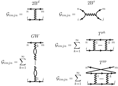
Figure 3: Top: Diagrams for the 2B^d (left) and 2B^x (right) methods. Bottom: Diagrams for the GW (left), $T^{ph}$ (top-right) and $T^{pp}$ (bottom right) methods.

Table 1: Definitions of electronic two-particle tensors. The vertically grouped indices are combined into one (greek) super-index.

Quantity	$\text{2B and }GW$	$T^{ph}$	$T^{pp}$
$\bm{\mathcal{G}}^{ee}_{\begin{subarray}{c}13\\ 24\end{subarray}}$	$\mathcal{G}^{ee}_{1423}$	$\mathcal{G}^{ee}_{1432}$	$\mathcal{G}^{ee}_{1234}$
$\mathbfit{h}^{e}_{\begin{subarray}{c}13\\ 24\end{subarray}}$	$h^{e}_{13}\delta_{42}-\delta_{13}h^{e}_{42}$	$h^{e}_{13}\delta_{42}-\delta_{13}h^{e}_{42}$	$h^{e}_{13}\delta_{24}+\delta_{13}h^{e}_{24}$
$\mathbfit{v}_{\begin{subarray}{c}13\\ 24\end{subarray}}$	$v_{1432}$	$v_{1423}$	$v_{1243}$
$\bm{\rho}^{\lessgtr}_{\begin{subarray}{c}13\\ 24\end{subarray}}$	$\rho^{\lessgtr}_{13}\rho^{\gtrless}_{42}$	$\rho^{\lessgtr}_{13}\rho^{\gtrless}_{42}$	$\rho^{\lessgtr}_{13}\rho^{\lessgtr}_{24}$

In Fig. 3 (top) we show the diagrammatic representation of the two-particle GF $\mathcal{G}^{ee}_{imjn}$ in the 2B^d and 2B^x approximation. They are obtained one from another by interchanging the external outgoing vertices $j$ and $n$. Alternatively, we can obtain one from another by exchanging the internal outoing (or incoming) vertices of the interaction line. The sum 2B${}^{d}+$2B^x is usually named the second-Born (2B) approximation. The two-particle GF in the $GW$, $T^{ph}$ and $T^{pp}$ approximation is illustrated in Fig. 3 (bottom). In Ref. [20] we proved that if one defines the matrices in the two-electron space as shown in Table 1 then $\bm{\mathcal{G}}^{ee(c)}$ satisfies the EOM

$$i\frac{d}{dt}\bm{\mathcal{G}}^{ee(c)} =-\bm{\Psi}^{e(c)}+\mathbfit{h}^{e(c)}_{\rm eff}\bm{\mathcal{G}}^{ee(c)}-\bm{\mathcal{G}}^{ee(c)}\mathbfit{h}^{e(c)\dagger}_{\rm eff},$$ (1aqa)

$$\bm{\Psi}^{e(c)} =\bm{\rho}^{>(c)}\mathbfit{v}^{(c)}\bm{\rho}^{<(c)}-\bm{\rho}^{<(c)}\mathbfit{v}^{(c)}\bm{\rho}^{>(c)},$$ (1aqb)

$$\mathbfit{h}^{e(c)}_{\rm eff} =\mathbfit{h}^{e(c)}-\bm{\rho}^{\Delta(c)}\mathbfit{v}^{\prime(c)},$$ (1aqc)

where the matrices $\mathbfit{v}^{(c)}$ and $\mathbfit{v}^{\prime(c)}$ are constructed from the four-index tensors

$$v^{(c)}_{ijmn} =a_{c}v_{ijmn}-b_{c}v_{ijnm},$$ (1ara)

$$v^{\prime(c)}_{ijmn} =a^{\prime}_{c}v_{ijmn}-b^{\prime}_{c}v_{ijnm}.$$ (1arb)

Table 2: Classes and parameters for all methods

Method	${\rm class}$	$a_{c}$	$b_{c}$	$a^{\prime}_{c}$	$b^{\prime}_{c}$
${\rm 2B}^{d}$	${\rm 2B}$	$1$	$0$	$0$	$0$
${\rm 2B}^{x}$	${\rm 2B}$	$0$	$1$	$0$	$0$
$GW$	$GW$	$1$	$0$	$1$	$0$
$GW^{x}$	$GW$	$0$	$1$	$1$	$0$
$XGW$	$GW$	$0$	$1$	$0$	$1$
$GW+X$	$GW$	$1$	$1$	$1$	$1$
$T^{ph}$	$T^{ph}$	$1$	$0$	$-1$	$0$
$T^{phx}$	$T^{ph}$	$0$	$1$	$-1$	$0$
$XT^{ph}$	$T^{ph}$	$0$	$1$	$0$	$-1$
$T^{ph}+X$	$T^{ph}$	$1$	$1$	$-1$	$-1$
$T^{pp}$	$T^{pp}$	$1$	$0$	$-1$	$0$
$T^{ppx}$	$T^{pp}$	$0$	$1$	$-1$	$0$

In Table 2 we report the values of $a_{c}$, $b_{c}$, $a^{\prime}_{c}$, $b^{\prime}_{c}$. Notice that to the first order in $v$ the nonperturbative methods ($GW$, $T^{ph}$ and $T^{pp}$) reduce to 2B^d. Henceforth the matrices in the two electron space are constructed as illustrated in Table 1 for all methods “$c$” belonging to the same “class”, see Table 2.

Exchange effects can be included in different ways. In analogy with the 2B method we could either exchange the outgoing vertices $j$ and $n$ or exchange the internal outgoing (or incoming) vertices of the interaction lines. Exchanging the incoming vertices $j$ and $n$ in $GW$, $T^{ph}$ and $T^{pp}$ leads to the $GW^{x}$, $T^{phx}$ and $T^{ppx}$ approximations illustrated in Fig. 4. Arranging the indices of the matrices according to the class these methods belong to ($GW^{x}$ like $GW$, $T^{phx}$ like $T^{ph}$ and $T^{ppx}$ like $T^{pp}$) we find again the EOM (1aq) with parameters given in Table 2. We observe that $h^{e(c)}_{\rm eff}$ is the same for the direct and exchange methods of the same class (same $a^{\prime}_{c}$ and $b^{\prime}_{c}$ parameters). This implies that if we are interested in treating correlations at the level of $2B=2B^{d}+2B^{x}$ or $GW+GW^{x}$ or $T^{ph}+T^{phx}$ or $T^{pp}+T^{ppx}$ we can sum the EOM for the direct and exchange methods, and propagate just one equation. The resulting EOM for the sum of the direct and exchange $\bm{\mathcal{G}}^{ee(c)}$ is the same as the EOM of the only-direct or only-exchange method but $\bm{\Psi}^{e}$ is calculated with $a_{c}=b_{c}=1$.

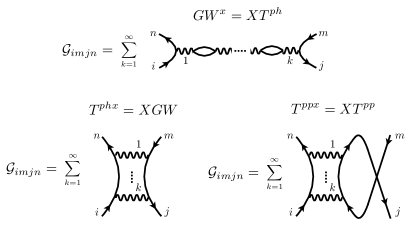
Figure 4: Top: Diagrams for the $GW^{x}=XT^{ph}$ method. Bottom: Diagrams for the $T^{phx}=XGW$ (left) and $T^{ppx}$ (left) methods.

Alternatively we can exchange the indices of the internal incoming (or outgoing) vertices of the interaction lines. Graphically this exchange amounts to replace the 2B^d-like structures with the 2B^x ones and viceversa. If we apply this graphical rule to $GW$ we obtain the $XGW$ approximation which is identical to $T^{phx}$. Similarly, if we apply the graphical rule to $T^{ph}$ we obtain the $XT^{ph}$ approximation which is identical to $GW^{x}$. Arranging the indices like in $GW$ for $XGW$ and like in $T^{ph}$ for $XT^{ph}$ we find the EOM (1aq) with parameters given in Table 2.

The $T^{pp}$ diagrams behave differently. Under the exchange of the internal incoming (or outgoing) vertices of the interaction lines a $T^{pp}$ diagram of order $n$ is mapped onto the same diagram if $n$ is even and onto the diagram of order $n$ of $T^{ppx}$ if $n$ is odd. Although this is a legitimate approximation it complicates the discussion on the double counting. We therefore do not address it further and write equivalently $T^{ppx}$ or $XT^{pp}$.

The inclusion of exchange effects like in $XGW$ and $XT^{ph}$ allows for constructing new approximations. If we replace every interaction line $v_{ijmn}$ with the difference $(v_{ijmn}-v_{ijnm})$ then $GW\to GW+X$ and $T^{ph}\to T^{ph}+X$ [20]. Graphically this amounts to replace every 2B^d structure with the 2B${}^{d}+$ 2B^x structure. The $GW+X$ and $T^{ph}+X$ approximations solve the Bethe-Salpeter equation (BSE) with Hartree-Fock kernel in the two inequivalent particle-hole channels. The standard BSE used to calculate absorption spectra corresponds to the $GW+X$ method [59]. The EOM for these approximations are again given by Eq. (1aq) with parameters given in Table 2.

Appendix D How to combine different methods without double counting

We have seen in the previous Section that the index order of the matrices in Eq. (1ia) is common to all methods belonging to the same “class” (2B, $GW$, $T^{ph}$ or $T^{pp}$) [20], and for $c$ in a given class the matrix elements of $\mathbfit{v}$ (appearing in $\bm{\Psi}^{e}$ and $\mathbfit{h}^{e}_{\rm eff}$) are calculated from the Coulomb tensor $v^{(c)}_{ijmn}=a_{c}v_{ijmn}-b_{c}v_{ijnm}$ (for $\bm{\Psi}^{e}$) and $v^{\prime(c)}_{ijmn}=a^{\prime}_{c}v_{ijmn}-b^{\prime}_{c}v_{ijnm}$ (for $\mathbfit{h}^{e}_{\rm eff}$). The integers $a_{c},b_{c}$ and $a^{\prime}_{c},b^{\prime}_{c}$ take values between $-1$ and $1$, see again Table 2.

The most convenient way to avoid double countings is to treat the four integers $n_{GW+X}$, $n_{T^{ph}+X}$, $n_{T^{pp}}$ and $n_{XT^{pp}}$ as independent and with values either 0 or 1. All other integers $n_{c}$ can then be chosen taking into account whether the method “$c$” is already included. For instance if $n_{GW+X}=1$ then $n_{GW}=-1,0$ whereas if $n_{GW+X}=0$ then $n_{GW}=0,1$. We then have the following possibilities

$$n_{GW} =-n_{GW+X},1-n_{GW+X},$$

$$n_{XGW} =-n_{GW+X},1-n_{GW+X},$$

$$n_{T^{ph}} =-n_{T^{ph}+X},1-n_{T^{ph}+X},$$

$$n_{XT^{ph}} =-n_{T^{ph}+X},1-n_{T^{ph}+X}.$$

The possible values of $n_{{\rm 2B}^{d}}$ can instead be $-N_{d},1-N_{d}$ where $N_{d}$ is the number of times that the second-order direct term is included: $N_{d}=n_{GW}+n_{GW+X}+n_{T^{ph}}+n_{T^{ph}+X}+n_{T^{pp}}$. Similarly $n_{{\rm 2B}^{x}}=-N_{x},1-N_{x}$ where $N_{x}$ is the number of times that the second-order exchange term is included: $N_{x}=n_{XGW}+n_{GW+X}+n_{XT^{ph}}+n_{T^{ph}+X}+n_{XT^{pp}}$.

Appendix E Numerical details

To isolate the correlation-induced charge migration of the Gly I conformer resulting from the removal of an electron from the $12a^{\prime}$ MO it is sufficient to consider the four MOs $12a^{\prime}$ (HOMO-8), $4a^{\prime\prime}$ (HOMO-2), $16a^{\prime}$ (HOMO) and $5a^{\prime\prime}$ (LUMO) [50, 51, 52, 53, 20]. Freezing all other electrons and working in the Hartree-Fock (HF) MO basis the electronic Hamiltonian in second quantization reads

$$\hat{H}_{\rm el} =\sum_{ij\sigma}\big{(}\delta_{ij}\epsilon^{\rm HF}_{i}-V^{\rm HF}_{ij}\big{)}\hat{d}^{{\dagger}}_{i\sigma}\hat{d}_{j\sigma}$$

$$+\frac{1}{2}\sum_{ijmn}\sum_{\sigma\sigma^{\prime}}v_{ijmn}\hat{d}^{{\dagger}}_{i\sigma}\hat{d}^{{\dagger}}_{j\sigma^{\prime}}\hat{d}_{m\sigma^{\prime}}\hat{d}_{n\sigma},$$ (1bf)

where $\epsilon^{\rm HF}_{i}=(-0.704,-0.475,-0.400,0.176)$ a.u. are the HF single-particle energies of the neutral molecule and $V^{\rm HF}$ is the HF potential generated by the active electrons; the sums run over spin and the four MOs. The shake-up process is activated by the Coulomb integral $v_{16a^{\prime}4a^{\prime\prime}5a^{\prime\prime}12a^{\prime}}=0.017$ a.u. and other integrals connected to it by the symmetry relations (for real MOs)

$$v_{ijmn}=v_{imjn}=v_{njmi}=v_{jinm}.$$ (1bg)

The renormalization of the energy of the shake-up state is instead mainly due to the direct integral $v^{d}_{4a^{\prime\prime}5a^{\prime\prime}}\equiv v_{4a^{\prime\prime}5a^{\prime\prime}5a^{\prime\prime}4a^{\prime\prime}}=0.39$ a.u., exchange integral $v^{x}_{4a^{\prime\prime}5a^{\prime\prime}}\equiv v_{4a^{\prime\prime}5a^{\prime\prime}4a^{\prime\prime}5a^{\prime\prime}}=0.08$ a.u. and all other integrals connected to these two through the symmetry relations in Eq. (1bg). The renormalization due to $v^{d}_{4a^{\prime\prime}5a^{\prime\prime}}$ is captured by the $XGW$ approximation whereas the renormalization due $v^{x}_{4a^{\prime\prime}5a^{\prime\prime}}$ is captured by the $GW$ approximation [20]. To simplify the discussion we have discarded $v^{d}_{4a^{\prime\prime}5a^{\prime\prime}}$; no complication arises in adding exchange to the $G\tilde{W}$ method.

To describe the molecule in a cavity we add to the reduced electronic Hamiltonian in Eq. (1bf) the free-photon Hamiltonian and the electron-photon interaction

$$\hat{H}_{\rm cavity}=\omega_{0}(\hat{a}^{{\dagger}}\hat{a}+\frac{1}{2})+\sum_{ij\sigma}\frac{g_{ij}}{\sqrt{2}}\hat{d}^{{\dagger}}_{i\sigma}\hat{d}_{j\sigma}(\hat{a}^{{\dagger}}+\hat{a}).$$ (1bh)

We study the case of a cavity-photon coupled to the transition $\Psi_{\rm shake-up}\to\Psi_{\rm cation}$ and therefore choose $g_{ij}=g_{ji}=g\neq 0$ only for the pair $4a^{\prime\prime}$ and $5a^{\prime\prime}$ of MOs. As detailed in the main text $g=\lambda d_{4a^{\prime\prime},5a^{\prime\prime}}\sqrt{\omega_{0}}$, where $d_{4a^{\prime\prime},5a^{\prime\prime}}=0.125$ a.u. is the dipole moment (averaged over three orthogonal directions) and $\lambda=0.212$ a.u.. is the electron-photon coupling strength [yang_quantum_2021].

In CI we first calculate the ground state $\Psi_{g}$ of the molecule in the cavity. At convergence the number of photons $n_{\rm ph}=\langle\Psi_{g}|\hat{a}^{{\dagger}}\hat{a}|\Psi_{g}\rangle$ is of the order of $10^{-4}$, consistent with the fact that cavity-photons are emitted only in the transition between cationic states. To ionize the molecule from the $12a^{\prime}$ MO we couple this state to a fictitious vacuum state

$$\hat{H}_{\rm laser}(t)=\sum_{\sigma}R(t)\,(\hat{d}^{{\dagger}}_{12a^{\prime}\sigma}\hat{d}_{\rm vacuum\,\sigma}+{\rm h.c.})$$ (1bi)

where the Rabi coupling

$$R(t)=R_{0}\theta(t)\theta(\tau-t)\sin^{2}(\frac{\pi t}{\tau})\sin(\omega_{\rm laser}t)$$ (1bj)

describes a laser pulse of duration $\tau$ centered at frequency $\omega_{\rm laser}$. The intensity $R_{0}$ is chosen small enough to work in the linear response regime, hence we check that the population of the $12a^{\prime}$ MO just after the pulse satisfies $\delta n_{12a^{\prime}}\equiv n_{12a^{\prime}}(\tau)-n_{12a^{\prime}}(0)={\mathcal{O}}(R_{0}^{2})$. We solve the time-dependent Schrödinger equation

$$i\frac{d}{dt}|\Psi(t)\rangle=\big{(}\hat{H}_{\rm el}+\hat{H}_{\rm cavity}+\hat{H}_{\rm laser}(t)\big{)}|\Psi(t)\rangle$$ (1bk)

with initial condition $|\Psi(t)\rangle=|\Psi_{g}\rangle$ for different photon frequencies $\omega_{0}$. In Fig. 2(d) we show the Fourier transform of $n_{12a^{\prime}}(t)=\sum_{\sigma}\langle\Psi(t)|\hat{d}^{{\dagger}}_{12a^{\prime}\sigma}\hat{d}_{12a^{\prime}\sigma}|\Psi(t)\rangle$.

In the GKBA+ODE we use the fact that the ground state $\Psi_{g}$ is weakly correlated and we approximate it with the HF ground-state with no photons. How to discard initial correlations in GKBA+ODE has already been discussed in Ref. [20]. In short this is done by calculating the electronic driving $\bm{\Psi}^{e}(t)$ defined in Eq. (1j) using only the shake-up Coulomb integrals and by setting to zero the bosonic driving $\bm{\Psi}^{b}(t)$ defined in Eq. (1k). The initial conditions for the bosonic displacements and density matrix describing an initial state with no photons are

$$\phi_{\xi}(0)=0,\quad\quad\gamma_{\xi\xi^{\prime}}(0)=\frac{1}{2}\left(\begin{array}[]{cc}1&-i\\ i&1\end{array}\right)_{\xi\xi^{\prime}}.$$ (1bn)

The initial condition for the electronic density matrix describing the photoionized molecule from the $12a^{\prime}$ MO is taken as

$$\rho(0)={\rm diag}(1-\frac{\delta n_{12a^{\prime}}}{2},2,2,0),$$ (1bo)

where $\delta n_{12a^{\prime}}$ is the depopulation obtained from the CI calculation. The initial condition for the high order GFs is simply $\bm{\mathcal{G}}^{ee}=\bm{\mathcal{G}}^{eb}=\bm{\mathcal{G}}^{b}=\bm{\mathcal{A}}=0$. It is straightforward to verify that for $\delta n_{12a^{\prime}}=0$ this set of initial conditions are a stationary solution of the GKBA+ODE equations for all methods. In Fig. 2(d) we show the Fourier transform of $n_{12a^{\prime}}(t)=\rho_{12a^{\prime}12a^{\prime}}(t)$ in three different diagrammatic approximations.