DISTAL: The Distributed Tensor Algebra Compiler

Abstract.

We introduce DISTAL, a compiler for dense tensor algebra that targets modern distributed and heterogeneous systems. DISTAL lets users independently describe how tensors and computation map onto target machines through separate format and scheduling languages. The combination of choices for data and computation distribution creates a large design space that includes many algorithms from both the past (e.g., Cannon’s algorithm) and the present (e.g., COSMA). DISTAL compiles a tensor algebra domain specific language to a distributed task-based runtime system and supports nodes with multi-core CPUs and multiple GPUs. Code generated by DISTAL is competitive with optimized codes for matrix multiply on 256 nodes of the Lassen supercomputer and outperforms existing systems by between 1.8x to 3.7x (with a 45.7x outlier) on higher order tensor operations.

1. Introduction

Tensor algebra kernels are key components of many workloads that benefit from the compute, memory bandwidth and memory capacity offered in a distributed system. However, the implementation of distributed tensor algorithms that are both correct and achieve high performance is a challenging task for most programmers. The situation is even more daunting when taking into account the heterogeneity within a single compute node; in many high performance systems today, managing the non-uniform memory access costs between the multiple GPUs and CPU sockets within a node is another distributed systems challenge to solve.

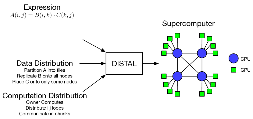
Figure 1. Example of the user-specified input (tensor algebra expressions, desired data and computation distribution) and output (code targeting supercomputers) of DISTAL.

We present DISTAL, a compilation-based system that provides novel abstractions to create implementations of any dense tensor algebra expression for modern heterogeneous machines. Figure 1 depicts how DISTAL lets users describe how the data and computation of a tensor algebra expression map onto a target machine. Figure 2 shows C++ code that implements a multi-GPU distributed matrix-multiply using DISTAL. Lines 4–15 map tensors onto the machine as part of the tensors’ format, and lines 23–LABEL:fig:lang-sample:line:sched-end map computation onto the machine through a loop transformation-based scheduling language. By separating the specifications of data distribution and computation distribution, DISTAL allows for their independent optimization, or for adapting either the data or computation distributions to complement the other.

Defining the distribution of both data and computation creates a design space of algorithms for each tensor computation. In particular, many algorithms from the literature are expressible as data distributions and schedules in DISTAL, including all of the algorithms in Figure 12 (Section 4). The abstractions of DISTAL let these algorithms be expressed with the expected asymptotic behavior and excellent practical performance. In fact, our evaluation (Section 7) demonstrates that implementations of these algorithms using DISTAL are competitive with hand-tuned implementations.

Implementations of tensor algebra operations on modern hardware can be hundreds to thousands of lines of low-level code that manage data movement between nodes and accelerators. For example, a conservative estimate of the core distributed matrix-multiplication logic in the implementation of the COSMA (Kwasniewski et al., 2019) algorithm by the original authors is around 500 lines of code, excluding lower-level communication code, local GEMM operations, whitespace, and comments. In contrast, the full data placement and distribution related scheduling for a GEMM using DISTAL is 15 lines of code (in Figure 2), while delivering competitive performance.

Alternatively to hand-coded implementations, state-of-the-art distributed tensor algebra libraries such as the Cyclops Tensor Framework (CTF) (Solomonik et al., 2014) achieve generality by decomposing tensor algebra expressions into a series of distributed matrix multiplication and transposition operations, relying on the efficiency of a hand-written set of core implementations. These approaches cannot implement the best algorithm for every tensor expression, as writing a hand-tuned implementation for every situation is impractical. With DISTAL, users can generate bespoke implementations of their tensor expressions that implement either algorithms from the literature or new algorithms tuned to a target machine.

Additionally, tensor algebra kernels that run on a distributed machine do not exist in a vacuum. These kernels operate on and generate data in the context of a larger application that imposes constraints on how the program’s data is partitioned and distributed among different memories in the target machine. Libraries such as ScaLAPACK (Choi et al., 1992) offer a set of kernels that assume a specific set of input distributions and require the user to reorganize their data into one of these distributions, which can result in additional data movement. In contrast, DISTAL lets users specialize computation to the way that data is already laid out, or easily transform data between distributed layouts to match the computation.

We implement DISTAL by extending the dense functionality in the TACO (Kjolstad et al., 2017) compiler to target the Legion (Bauer et al., 2012) distributed runtime system, as shown in Figure 3. We extend the format and scheduling languages of TACO with primitives for distribution. Next, we add analysis passes and intermediate representation constructs to TACO to generate Legion programs that interface with a mapper that places data and computation onto memories and processors.

The specific contributions of this work are:

1. A data distribution language and set of scheduling commands that can express a wide variety of distributed tensor computations.

2. A compiler that combines the separate specifications for how data and computation map onto distributed machines.

3. An implementation of DISTAL that extends the TACO (Kjolstad et al., 2017) compiler to target the Legion (Bauer et al., 2012) runtime system.

We evaluate our contributions along two different axes:

Generality. We implement several tensor algebra kernels and show that we achieve good performance. We show that our approach of generating bespoke implementations achieves between a 1.8x to 3.7x (with a 45.7x outlier) speedup over CTF, a system aimed at a similar level of generality.

Absolute Performance. Our system matches or outperforms existing systems on dense matrix-matrix multiplication, a tensor algebra operation that has been extensively optimized in prior work. In particular, dense matrix multiplication code generated by DISTAL outperforms the CTF (Solomonik et al., 2014) and ScaLAPACK (Choi et al., 1992) libraries by at least 1.25x and comes within 0.95x the performance of COSMA (Kwasniewski et al., 2019), the best published dense matrix-matrix multiplication implementation.

⬇

1// Declare input parameters for generated code.

2Param gx, gy, n, chunkSize;

3// Define the target machine m as a 2D grid of processors.

4Machine m(Grid(gx, gy));

5

6// A tensor’s format describes how it is distributed onto m.

7// The following format partitions the two dimensions of a tensor by

8// the two dimensions of m, resulting in a two-dimensional tiling.

9// The final argument declares the tensor should reside in GPU

10// framebuffer memory for fast access from GPUs.

11Distribution tiles(m, {0, 1}, Memory::GPU_MEM); // (x, y) -> m(x, y)

12Format f({Dense, Dense}, tiles);

13

14// Declare three dense matrices with the same format.

15Tensor<double> A({n, n}, f), B({n, n}, f), C({n, n}, f);

16

17// Declare the computation, a matrix-matrix multiply.

18IndexVar i, j, k;

19A(i, j) = B(i, k) * C(k, j);

20

21// Map the computation onto m via scheduling commands.

22IndexVar io, ii, jo, ji, ko, ki;

23A.schedule()

24 // Tile i and j for each GPU.

25 .divide(i, io, ii, m.x).divide(j, jo, ji, m.y)

26 .reorder({io, jo, ii, ji})

27 // Distribute each i and j tile over all GPUs.

28 .distribute(io).distribute(jo)

29 // Break the k loop into chunks.

30 .split(k, ko, ki, chunkSize)

31 // Move the outer k loop to outside the ii and ji loops.

32 .reorder({io, jo, ko, ii, ji, ki})

33 // Choose the granularity at which communication occurs.

34 // Here, each processor operates on a local piece of a, and

35 // receives chunks of b and c as the ko loop steps.

36 .communicate(a, jo).communicate({b, c}, ko)

37 // Schedule at leaves for variables ii, ji, and ki. Our

38 // system can generate code for GPUs, but allows for using

39 // heavily optimized kernels when applicable.

40 .substitute({ii, ji, ki}, CuBLAS::GeMM)\label{fig:lang-sample:line:sched-end};

Figure 2. Multi-GPU matrix multiplication in DISTAL implementing the SUMMA (van de Geijn and Watts, 1995) algorithm used by ScaLAPACK (Choi et al., 1992).

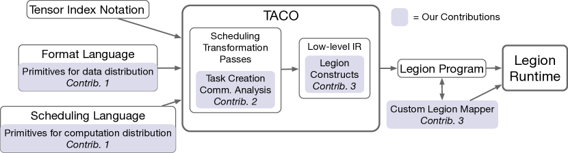
Figure 3. Overview of DISTAL’s implementation.

2. Background

Figure 2 shows DISTAL’s three input sub-languages: a computation language that describes the desired kernel (lines 18–19), a scheduling language that describes how to optimize the computation (lines 23–LABEL:fig:lang-sample:line:sched-end), and a format language that describes how the tensors are stored (lines 4–15). In this section, we give background on each of these three components.

Computation is described in DISTAL using tensor index notation, a domain specific language used as input to the TACO compiler (Kjolstad et al., 2017). Tensor index notation consists of accesses that index tensor dimensions with lists of variables. Tensor index notation statements are assignments, where the left-hand side is an access, and the right-hand side is an expression constructed from the addition and multiplication of accesses. For example, the tensor-times-vector operation is expressed in tensor index notation as $A(i,j)=\sum_{k}B(i,j,k)\cdot c(k)$. Each component $A(i,j)$ is the result of the inner-product of the last dimension of $B$ with $c$. Index variables correspond to nested loops, and variables used only on the right-hand side represent sum reductions over their domain. Tensor index notation allows for any number of tensors on the right-hand side of an expression, and, like TACO, DISTAL can generate a single fused kernel for the entire tensor index notation expression.

The computation description is separated from the exact algorithm to perform the computation through a scheduling language (Ragan-Kelley et al., 2013; Zhang et al., 2018; Chen et al., 2018; Vasilache et al., 2018; Baghdadi et al., 2018; Senanayake et al., 2020). We provide the following transformations introduced by prior systems (Ragan-Kelley et al., 2013; Senanayake et al., 2020; Kjolstad et al., 2019):

• parallelize: parallelize the iterations of a loop

• split/divide: break a loop into an inner and outer loop

• collapse: fuse two nested loops into a single loop

• reorder: switch the execution order of two loops

• precompute: hoist the computation of a subexpression

We will introduce three new scheduling commands that describe how computations map onto a distributed machine.

Moreover, the TACO (Kjolstad et al., 2017) compiler introduced a format language that allows users to specify the sparse format of each tensor in a computation. While this work considers only dense computations, we take inspiration from TACO to describe a tensor’s distribution as part of the tensor’s format.

3. Core Abstractions

This section describes the core abstractions of DISTAL that allow users to express a virtual machine organization and to map data and computation onto that machine.

3.1. Modeling Modern Machines

DISTAL models a distributed machine $\mathcal{M}$ as a multidimensional grid of abstract processors that each have an associated local memory and can communicate with all other processors. The purpose of the grid abstraction is twofold: to expose locality in the model (which may or may not exist in the physical machine) and to match the grid-like structure of tensor algebra computations.

A flat machine representation is useful, but is not sufficient to model many modern high performance systems. These systems are often heterogeneous, where each node contains multiple accelerators and CPU sockets that offer faster communication within a node than between nodes. Therefore, our machine abstraction is also hierarchical: each abstract processor may itself be viewed as a distributed machine. We use this abstraction in our evaluation to model the Lassen supercomputer; we arrange the nodes into multi-dimensional grids, then model each node as a grid of GPUs.

$$\begin{array}[]{rlrlrl}\textit{Machines}&\mathcal{M}&\textit{Tensors}&\mathcal{T}&\textit{Dimension Variables}&d\\ \end{array}$$

$$\begin{array}[]{rlcl}\textit{Dimension Name}&n&\mathrel{::=}&d\mathrel{\mid}\mathbb{N}\mathrel{\mid}\text{'$*$'}\\ \textit{Tensor Distribution}&\mathcal{D}&\mathrel{::=}&\mathcal{T}\operatorname{{\vphantom{\mapsto}}_{d^{+}}\kern-0.5pt\mathnormal{\mapsto}_{n^{+}}}\mathcal{M}\\ \end{array}$$

Figure 4. Syntax of Tensor Distribution Notation

Figure 5. Blocked distribution of a vector.

Figure 6. Row-wise matrix distribution.

Figure 7. Tiled matrix distribution.

(a) Fix a partition to a dimension.

(b) Broadcast a partition over a dimension.

(c) Map a 3-tensor onto a processor grid.

Figure 8. Examples of tensor distribution notation statements that map tensors onto machines in different ways.

3.2. Data Distribution

Users map tensors onto machines through a sub-language of the format language called tensor distribution notation. Tensor distribution notation allows users to describe how input tensors are already distributed in their program or to move data into a distributed layout that suits the computation.

Syntax. Figure 4 describes the syntax for tensor distribution notation, which encodes how dimensions (modes) of a tensor $\mathcal{T}$ map onto the dimensions of a machine $\mathcal{M}$. Tensor distribution notation expresses this mapping by naming each dimension of $\mathcal{T}$ and $\mathcal{M}$; index sequences on the left and right of the $\mapsto$ name dimensions in $\mathcal{T}$ and $\mathcal{M}$ respectively. Tensor dimensions that share names with machine dimensions are partitioned across those machine dimensions. The remaining machine dimensions broadcast the partition over the dimensions, or fix the partition to a coordinate in the dimension. A tensor distribution notation statement $\mathcal{T}\operatorname{{\vphantom{\mapsto}}_{X}\kern-0.5pt\mathnormal{\mapsto}_{Y}}\mathcal{M}$, where X and Y are index sequences, is valid if $|X|=\dim\mathcal{T}$, $|Y|=\dim\mathcal{M}$, both $X$ and $Y$ contain no duplicate names, and all names in $Y$ are present in $X$.

Intuition. Tensor dimensions partitioned across machine dimensions are divided into equal-sized contiguous pieces. For example, if $\mathcal{T}$ and $\mathcal{M}$ are one-dimensional with 100 components and 10 processors respectively, then the distribution $\mathcal{T}\operatorname{{\vphantom{\mapsto}}_{x}\kern-0.5pt\mathnormal{\mapsto}_{x}}\mathcal{M}$ maps 10 components of $\mathcal{T}$ to every processor of $\mathcal{M}$. Many common blocked partitioning strategies can be expressed by the choice of tensor dimensions to partition. Figure 8 displays multiple ways of partitioning a matrix, such as by rows ($\mathcal{T}\operatorname{{\vphantom{\mapsto}}_{xy}\kern-0.5pt\mathnormal{\mapsto}_{x}}\mathcal{M}$, Figure 6), by columns ($\mathcal{T}\operatorname{{\vphantom{\mapsto}}_{xy}\kern-0.5pt\mathnormal{\mapsto}_{y}}\mathcal{M}$), or by two-dimensional tiles ($\mathcal{T}\operatorname{{\vphantom{\mapsto}}_{xy}\kern-0.5pt\mathnormal{\mapsto}_{xy}}\mathcal{M}$, Figure 7). Tensor dimensions that are not partitioned span their full extent in each partitioned piece, as seen in Figure 6 and 7(c).

Machine dimensions that do not partition tensor dimensions either fix the tensor to a single index or broadcast the tensor across all indices of a dimension. A tensor is fixed to a single machine index by naming the dimension with a constant as in $\mathcal{T}\operatorname{{\vphantom{\mapsto}}_{xy}\kern-0.5pt\mathnormal{\mapsto}_{xy0}}\mathcal{M}$ in 7(a), which restricts the tensor tiles to a face of the machine. Marking a dimension with a $*$ replicates a tensor across that dimension, such as $\mathcal{T}\operatorname{{\vphantom{\mapsto}}_{xy}\kern-0.5pt\mathnormal{\mapsto}_{xy*}}\mathcal{M}$ in 7(b) where tensor tiles are replicated across the entire third dimension of $\mathcal{M}$.

Semantics. Having described tensor distribution notation intuitively, we now provide a more formal description. We define a tensor $\mathcal{T}$ to be a set of coordinate–value pairs and a machine $\mathcal{M}$ to be a set of coordinates. A tensor distribution notation statement $\mathcal{T}\operatorname{{\vphantom{\mapsto}}_{X}\kern-0.5pt\mathnormal{\mapsto}_{Y}}\mathcal{M}$ is a function that maps the coordinates in $\mathcal{T}$ to a non-empty set of processor coordinates in $\mathcal{M}$, where $X$ and $Y$ are index sequences. This function is the composition of two functions $\mathcal{P}:\mathcal{T}\rightarrow\textsf{color}$ and $\mathcal{F}:\textsf{color}\rightarrow\mathcal{M}\leavevmode\nobreak\ \textsf{set}$. $\mathcal{P}$ is an abstract partitioning function that maps coordinates in $\mathcal{T}$ to unique colors. $\mathcal{F}$ then maps each color in the range of $\mathcal{P}$ to processors in $\mathcal{M}$. That is, we first group coordinates of $\mathcal{T}$ into equivalence classes (colors), and then map each equivalence class to a processor (or processors, if broadcast) in $\mathcal{M}$.

Let $p=X\cap Y$, the dimensions of $\mathcal{T}$ that are partitioned by dimensions of $\mathcal{M}$. Concretely, a color is a point in the $p\subseteq Y$ dimensions of $\mathcal{M}$. $\mathcal{P}$’s coloring is a many-to-one mapping between points in the $p$ dimensions of $\mathcal{T}$ and colors. The coloring is lifted to the remaining non-partitioned dimensions of $\mathcal{T}$ in the natural way: every coordinate $x\in\mathcal{T}$ is given the same color as $\mathcal{P}(x_{p})$, where $x_{p}$ is $x$ restricted to the $p$ dimensions of $\mathcal{T}$. We choose to use a blocked partitioning function that maps contiguous ranges of coordinates to the same color. However, other functions such as a cyclic distribution that maps adjacent coordinates to different colors could also be used. As a running example, consider the distribution $\mathcal{T}\operatorname{{\vphantom{\mapsto}}_{xy}\kern-0.5pt\mathnormal{\mapsto}_{xy*}}\mathcal{M}$ (7(b)), where $\mathcal{T}$ is 2x2 and $\mathcal{M}$ is 2x2x2. For this tensor distribution notation statement,

$$\mathcal{P}=\{(0,0)\mapsto(0,0),(0,1)\mapsto(0,1),(1,0)\mapsto(1,0),(1,1)\mapsto(1,1)\},$$

mapping the coordinates in the 2x2 matrix onto points in the first two dimensions of the 2x2x2 machine cube.

$\mathcal{F}$ maps $\mathcal{P}$’s coloring of $\mathcal{T}$ to full coordinates of processors in $\mathcal{M}$. As discussed previously, each color is an assignment to the $p\subseteq Y$ dimensions of $\mathcal{M}$ and can be mapped to a coordinate of a processor in $\mathcal{M}$ by specifying an index for the remaining $Y-p$ dimensions. Since all names in $Y$ must be present in $X$ as a condition of tensor distribution validity, the remaining $Y-p$ dimensions must either fix or broadcast the partition. $\mathcal{F}$ expands the color to the remaining dimensions of $\mathcal{M}$ by casing on whether each dimension fixes or broadcasts the partition: fixed dimensions are set to the target value and broadcasted dimensions are expanded to all possible coordinates in the dimension. In the running example,

$$\mathcal{F}=\{ (0,0)\mapsto\{(0,0,0),(0,0,1)\},(0,1)\mapsto\{(0,1,0),(0,1,1)\},$$

$$(1,0)\mapsto\{(1,0,0),(1,0,1)\},(1,1)\mapsto\{(1,1,0),(1,1,1)\}\},$$

expanding the coloring of $\mathcal{P}$ to the third dimension of $\mathcal{M}$.

Hierarchy. Data distributions can also be hierarchical to match the hierarchical structure of the machine. If the target machine has a hierarchical structure, then a tensor distribution can be provided for each level in the machine. For example, if the machine $\mathcal{M}$ is organized as a 2-dimensional grid at the node level, and then a 1-dimensional grid of GPUs within each node, then the distribution $[\mathcal{T}\operatorname{{\vphantom{\mapsto}}_{xy}\kern-0.5pt\mathnormal{\mapsto}_{xy}}\mathcal{M},\mathcal{T}\operatorname{{\vphantom{\mapsto}}_{zw}\kern-0.5pt\mathnormal{\mapsto}_{z}}\mathcal{M}]$ represents a two dimensional tiling of a matrix at the outer level, and row-wise partition of each tile for each GPU.

3.3. Computation Distribution

Like a tensor distribution notation statement describes how a tensor is distributed across a machine, a schedule describes how the iteration space of an expression is transformed and distributed. In this section, we introduce three new scheduling transformations on top of those introduced in the background section: distribute, communicate, and rotate. The first two were used in Figure 2. Throughout this section, we use the computation $a(i)=\sum_{j}b(j)$ as a running example, which has loop structure $\forall_{i}\forall_{j}\leavevmode\nobreak\ a(i)\mathrel{+}=b(j)$. This computation sets each index of $a$ to be the sum of all elements in $b$. In our examples, we consider a one-dimensional machine $\mathcal{M}$, where $A\operatorname{{\vphantom{\mapsto}}_{x}\kern-0.5pt\mathnormal{\mapsto}_{x}}\mathcal{M}$, $B\operatorname{{\vphantom{\mapsto}}_{x}\kern-0.5pt\mathnormal{\mapsto}_{x}}\mathcal{M}$ and $|A|=|B|=|\mathcal{M}|=3$.

Iteration Spaces. The iteration space of loops in a tensor algebra expression is a hyper-rectangular grid of points formed by taking the Cartesian product of the iteration domain of each index variable in the input expression. Each point in the iteration space represents a scalar operation that is the atomic unit of computation in our model.

Execution Spaces. We model the execution of an iteration space through an execution space, which describes when and where each iteration space point is executed. An execution space has a processor dimension and a time dimension, describing what processor an iteration space point executes on and at what relative time the point executes. A mapping of iteration space points onto an execution space describes an execution strategy for the iteration space. Each processor and point in time may be assigned one point $p$ in the iteration space as well as communication operations to fetch tensor data needed by $p$ that logically occur before $p$; we discuss communication operations below. An iteration space’s default execution space mapping linearizes all points in time according to the ordering of the iteration space dimensions and maps all points to the same processor.

Distribute. The distribute operation transforms how the iteration space maps onto the execution space. In particular, distribute-ing a set of index variables $v$ modifies the execution space mapping such that all iterations of the dimensions corresponding to $v$ occur on a different processors at the same time, as seen in Figure 9.

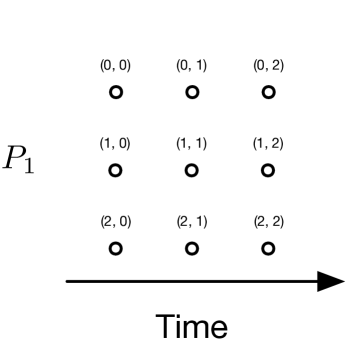
Figure 9. Execution space mapping of $\forall_{i}\forall_{j}\leavevmode\nobreak\ a(i)\mathrel{+}=b(j)$ after distribute(i). Iteration space points are labeled $(i,j)$.

The following compound command utilizes the distribute, divide and reorder commands to map a set of iteration space dimensions onto a machine by tiling the iteration space dimensions onto each processor in the machine:

⬇

1distribute(vector<IndexVar> targets, vector<IndexVar> dist,

2 vector<IndexVar> local, Machine m):

3 for i in range(0, m.dim):

4 # Divide each dimension by the corresponding machine dimension.

5 divide(targets[i], dist[i], local[i], m.dims[i])

6 # Reorder loops so each outer divided variable is on the outside.

7 reorder(dist + local)

8 # Distribute all of the outer divided variables.

9 distribute(dist)

The choice of variables to distribute affects the resulting communication patterns. Distributing variables that index the output tensor pull input tensors towards a stationary output tensor in an owner-computes paradigm. Distributing variables used for reductions results in distributed reductions into the output, trading space usage for increased parallelism.

To match hierarchical machine models and data distributions, distribute may also be applied hierarchically. For example, we can apply this strategy in computations that benefit from locality, like matrix-multiply, to use a distributed algorithm at the node level and another (sometimes different) algorithm for the multiple GPUs within a node.

Communicate. Every iteration space point maps to a coordinate in each of the input and output tensors, corresponding to the data required at that point. The data required at each iteration space point may not be present in the memory of the processor the point is mapped to, and must be communicated from a memory where the data resides. A communication operation will be automatically inserted at each execution space point where the required data is not present, resulting in a naïve completion of the execution space mapping. A naïve completion of the execution space of $\forall_{i}\forall_{j}\leavevmode\nobreak\ a(i)\mathrel{+}=b(j)$ transformed by distribute(i) is depicted in 10(a).

Communication operations can be made more efficient by aggregating them into larger operations that fetch the data for a group of iteration space points, as seen in 10(b). The choice of how much communication to aggregate incurs the tradeoff between memory usage and communication frequency—more frequent communication allows for lower memory usage at the cost of more messages sent.

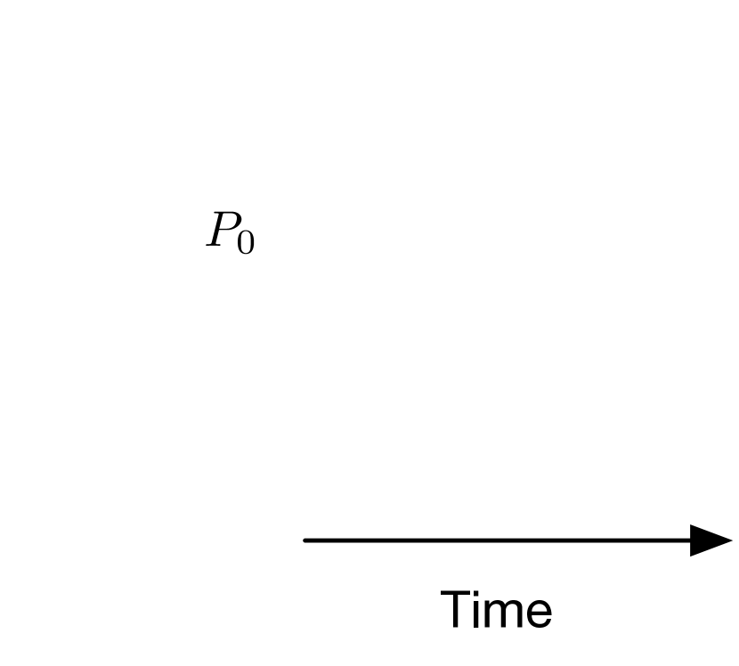
(a) Naïve completion where communication is inserted as needed at each iteration space point.

(b) Completion where communication is aggregated underneath each $i$ iteration.

Figure 10. Completions of the distributed execution space mapping of $\forall_{i}\forall_{j}\leavevmode\nobreak\ a(i)\mathrel{+}=b(j)$ where $a\operatorname{{\vphantom{\mapsto}}_{x}\kern-0.5pt\mathnormal{\mapsto}_{x}}\mathcal{M}$ and $b\operatorname{{\vphantom{\mapsto}}_{x}\kern-0.5pt\mathnormal{\mapsto}_{x}}\mathcal{M}$.

To allow for optimization over this tradeoff space, the communicate command controls how much communication for each tensor should be aggregated into a single message. Precisely, communicate($\mathcal{T}$, i) aggregates the communication of $\mathcal{T}$ at the beginning of each iteration of i by materializing the data for all iteration space points nested under each iteration of i in the executing processor’s memory. If no communicate command is given, then communication will be nested under the inner-most index variable.

It is a deliberate choice to omit any notion of processor ranks, explicit sends/receives, and specific channels used (such as in prior work (Baghdadi et al., 2018)) from the scheduling language so that schedules only affect performance, not correctness, as well as to keep the scheduling language relatively simple. The communicate command is not needed for correctness and is used only to optimize the communication pattern of the computation.

(a) Standard execution space mapping. At each time step, the processor $j$ broadcasts $b[j]$ to all other processors.

(b) Rotated execution space mapping. At each time step, each processor transfers the data received at the previous time step.

Figure 11. Communication (denoted by dashed arrows) between processors in execution space mappings for $\forall_{i}\forall_{j}\leavevmode\nobreak\ a(i)\mathrel{+}=b(j)$ with and without rotate.

Algorithm	Comm. Pattern	Target Machine	Data Distribution	Schedule
⬇ .distribute({i, j}, {io, jo}, {ii, ji}, Grid(gx, gy)) .divide(k, ko, ki, gx) .reorder({ko, ii, ji, ki}) .rotate(ko, {io, jo}, kos) .communicate(A, jo).communicate({B, C}, kos)
⬇ .distribute({i, j}, {io, jo}, {ii, ji}, Grid(gx, gy)) .divide(k, ko, ki, gx) .reorder({ko, ii, ji, ki}) .rotate(ko, {io}, kos) .communicate(A, jo).communicate({B, C}, kos)
⬇ .distribute({i, j}, {io, jo}, {ii, ji}, Grid(gx, gy)) .split(k, ko, ki, chunkSize) .reorder({ko, ii, ji, ki}) .communicate(A, jo).communicate({B, C}, ko)
⬇ .distribute({i, j, k}, {io, jo, ko}, {ii, ji, ki}, Grid($\sqrt[3]{p}$, $\sqrt[3]{p}$, $\sqrt[3]{p}$)) .communicate({A, B, C}, kn)
⬇ .distribute({i, j, k}, {io, jo, ko}, {ii, ji, ki}, Grid($\sqrt{\frac{p}{c}}$, $\sqrt{\frac{p}{c}}$, c)) .divide(ki, kio, kii, $\sqrt{\frac{p}{c^{3}}}$) .reorder({kio, il, jl, kii}) .rotate(kio, {io, jo}, kios) .communicate(A, jo).communicate({B, C}, kios)
⬇ // gx, gy, gz, numSteps computed by COSMA scheduler. .distribute({i, j, k}, {io, jo, ko} {ii, ji, ki}, Grid(gx, gy, gz)) .divide(ki, kio, kii, numSteps) .reorder({kio, il, jl, kii}) .communicate(A, ko).communicate({B, C}, kio)

Figure 12. Set of matrix-multiplication algorithms representable by DISTAL. For each algorithm, we show the high level communication pattern, target machine organization, initial data distributions, and schedule of the compute statement $A(i,j)=\sum_{k}B(i,k)\cdot C(k,j)$. In the icons, black arrows indicate communications for $A$, blue for $B$ and red for $C$. The schedules utilize the compound distribute command introduced in Subsection 3.3.

Rotate. Many distributed algorithms have a systolic communication pattern, where processors repeatedly shift data to their neighbors. Systolic algorithms can take advantage of machine architectures with interconnects that offer higher performance for nearest-neighbor communication and improve performance by avoiding contention for the same pieces of data. To express systolic computations, we introduce the rotate operation, which acts as a symmetry-breaking operation for distributed loops by transforming the mapping onto the time dimension of the execution space.

To gain intuition for rotate, consider the execution space mapping of the running example $\forall_{i}\forall_{j}\leavevmode\nobreak\ a(i)\mathrel{+}=b(j)$ transformed by distribute(i). At each time step, all processors access (and issue communication requests for) the same element of $B$, causing the owner of that element to broadcast it to all other processors, as seen in 11(a). In contrast, a systolic version of this computation would instead have each processor accumulate the local element of $b$, and then shift the local element to the processor to its left in $\mathcal{M}$.

The systolic communication pattern is achieved by changing the point in time that each processor executes each iteration of the $j$ loop. If the mapping of the time dimension is reordered such that for each iteration of $i$, the $j$ iteration space is rotated in time so that the $i$th iteration of $j$ occurs first, then the resulting execution space has a systolic communication pattern, where each processor utilizes the data that the processor to its right used in the previous iteration. This effect is depicted in 11(b) where no processors execute the same iteration of $j$ at the same point in time.

Concretely, given a set of index variables $I$, target index variable $t$ and result index variable $r$, rotate($t$, $I$, $r$) rotates each iteration of $t$ by $\sum_{i\in I}i\leavevmode\nobreak\ \textsf{mod extent}(t)$. The effect of rotate is that $\forall i\in I$, given a fixed iteration for all remaining $i^{\prime}\in(I-i)$, the same iteration of $r$ occurs at a different time for all iterations of $i$. For example, if $t$ is rotated by variables $i$ and $j$ oriented in a 2D grid, every row starts the iteration of $r$ at a unique value, and vice versa for each column.

4. Matrix-Multiplication Case Studies

Tensor distribution notation and scheduling can be composed to express a wide variety of algorithms. A large body of research on distributed tensor algebra focuses on algorithms for distributed matrix-multiplication. Therefore, to showcase the expressivity of our techniques, we perform a case study on matrix-multiplication algorithms discussed in the literature. However, our techniques are not specific to matrix-multiplication and generalize to all of tensor algebra.

4.1. Distributed Matrix-Multiplication Background

The first distributed matrix-multiplication algorithm, presented by Cannon (Cannon, 1969), uses a systolic communication pattern and a tiled distribution of the input matrices. The PUMMA (Choi et al., 1994) and SUMMA (van de Geijn and Watts, 1995) algorithms extended this work by generalizing to rectangular matrices and improving the communication patterns through pipelining. The SUMMA algorithm is implemented in the widespread ScaLAPACK (Choi et al., 1992) library. These are called 2D algorithms, because they organize the target machine into a 2D grid and decompose the input matrices in tiles on the processor grid.

Follow up work by Agrawal et al. (Agarwal et al., 1995) introduced Johnson’s algorithm, which organized processors into a 3D grid and utilized extra memory per processor to perform asymptotically less communication than 2D algorithms. Algorithms of this style are called 3D algorithms. The 2.5D algorithm by Solomonik et al. (Solomonik and Demmel, 2011) interpolates between 2D and 3D algorithms, utilizing extra memory to reduce communication. The 2.5D algorithm has been implemented in the Cyclops Tensor Framework (Solomonik et al., 2014). Finally, the COSMA (Kwasniewski et al., 2019) algorithm takes a different approach by computing an optimal processor organization and parallelization strategy depending on the target matrix dimensions and machine size.

Figure 12 depicts the communication pattern of these algorithms and demonstrates how each can be implemented in DISTAL. Although DISTAL cannot represent recursive algorithms like CARMA (Demmel et al., 2013), it still covers a space of widely used algorithms. We now present detailed derivations of SUMMA, Cannon’s and Johnson’s algorithms.

4.2. SUMMA

MPI-like pseudocode for SUMMA can be found in Figure 13. SUMMA organizes the computation into a 2D grid and each processor owns a tile of $A$, $B$, and $C$. Computation proceeds in chunks over the $k$ loop, where processors owning the $k$’th chunks of the $B$ and $C$ loops broadcast the chunks within their row and column respectively. Then, each processor multiplies the communicated chunks of $B$ and $C$ into a local tile of $A$.

⬇

# Arrange $p$ processors into a 2 D grid.

# Assign a tile of $A$, $B$, $C$ to each processor.

for all $P_{ ij} $ in parallel:

for kc in (0, k, chunkSize):

$B_l$ = row broadcast the kc to kc+ chunkSize columns of $B$

$C_l$ = col broadcast the kc to kc+ chunkSize rows of $C$

A += $B_l$ $\ times$ $C_l$

Figure 13. Pseudocode for the SUMMA algorithm.

SUMMA organizes the target machine as a 2D grid ($\mathcal{M}=\textsf{Grid(gx, gy)}$) and maps each tensor in tiles using $A\operatorname{{\vphantom{\mapsto}}_{xy}\kern-0.5pt\mathnormal{\mapsto}_{xy}}\mathcal{M}$, $B\operatorname{{\vphantom{\mapsto}}_{xy}\kern-0.5pt\mathnormal{\mapsto}_{xy}}\mathcal{M}$, and $C\operatorname{{\vphantom{\mapsto}}_{xy}\kern-0.5pt\mathnormal{\mapsto}_{xy}}\mathcal{M}$. The $i$ and $j$ iteration space dimensions are distributed, and every processor locally iterates through the $k$ dimension. Therefore, we apply distribute({i,j}, {io,jo}, {ii,ji}, Grid(gx,gy)). Next, SUMMA steps through $k$ in chunks expressible with split(k, ko, ki, chunkSize) followed by reorder({ko, ii, ji, ki}). Finally, we schedule the communication: since each processor operates on a tile of $A$, we communicate(A, jo). SUMMA broadcasts $B$ and $C$ in chunks along the $k$ loop, so we communicate under the ko outer loop using communicate({B, C}, ko).

This schedule implements SUMMA. Each processor steps over the $k$ dimension of the iteration space, and performs local matrix multiplications on chunks of $B$ and $C$. Every processor operates on the same chunks of $B$ and $C$ in its row and column, the processors that owns the chunks broadcast them to the other processors in their rows and columns.

4.3. Cannon’s Algorithm

As another 2D algorithm, Cannon’s algorithm has the same target machine and data distribution as SUMMA, but has a systolic communication pattern, as seen in Figure 14, where processors shift tiles along their row and column. Despite the differences in pseudocode, the schedule for Cannon’s algorithm is similar to the schedule for SUMMA’s. First, we change the split operation into divide(k, ko, ki, gx) so that the tiles communicated are the same size as the tiles held by each processor. Next, we change the communication pattern to the systolic pattern using rotate. We insert a rotate(ko, {io,jo}, kos) to rotate each processors ko iteration space by the processor’s coordinate in the processor grid. Figure 15 depicts the communication pattern of $B$ after rotation.

⬇

# Arrange $p$ processors into a 2 D grid, $\ sqrt{ p} \ times \ sqrt{ p} $.

# Assign a tile of $A$, $B$, $C$ to each processor.

# Perform an initial data shift.

for all $P_{ ij} $ in parallel:

shift $B_{ ij} $ $i$ spaces to the left

shift $C_{ ij} $ $j$ spaces upwards

for all $P_{ ij} $ in parallel:

for k in (0, $\ sqrt{ p} $):

$A_{ ij} $ += $B_{ ij} $ $\ times$ $C_{ ij} $

shift $B_{ ij} $ to the left

shift $C_{ ij} $ upwards

Figure 14. Pseudocode for Cannon’s algorithm.

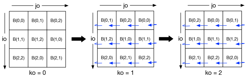
Figure 15. Communication pattern of $B$ in the Cannon’s algorithm schedule on a 3x3 grid of processors. $B(x,y)$ is the $(x,y)$th tile of $B$. At each iteration of ko, each processor performs the rotated iteration kos = ko + io + jo mod 3, accessing $B($io, kos$)$. Each processor is labeled with the tile of $B$ needed at the current iteration. Blue arrows indicate from where the data needed at the current iteration was sent.

4.4. Johnson’s Algorithm

Johnson’s algorithm is a 3D algorithm, so it has a different target machine and initial data distribution, as seen in Figure 16. Given $p$ processors, Johnson’s algorithm targets a processor cube with side length $\sqrt[3]{p}$: $\mathcal{M}=\textsf{Grid}(\sqrt[3]{p},\sqrt[3]{p},\sqrt[3]{p})$. The input matrices are partitioned into tiles, and then fixed to a face of the processor cube. We express the distribution of $A$ using $A\operatorname{{\vphantom{\mapsto}}_{xy}\kern-0.5pt\mathnormal{\mapsto}_{xy0}}\mathcal{M}$, which partitions $A$ by the first two dimensions of $\mathcal{M}$, and then fixes the partition onto a face of $\mathcal{M}$. The placements for $B$ and $C$ are similar, but restrict the matrices to different faces of the processor cube.

⬇

# Arrange $p$ processors into a 3 D grid, $\ sqrt[3]{ p} \ times \ sqrt[3]{ p} \ times \ sqrt[3]{ p} $.

# Assign a tile of $A$ to each processor $P_{ ij0} $.

# Assign a tile of $B$ to each processor $P_{ i0k} $.

# Assign a tile of $C$ to each processor $P_{0 jk} $.

for all $P_{ ijk} $ in parallel:

$P_{ i0k} $ broadcasts $B_{ ik} $ to each $P_{ ijk} $

$P_{0 jk} $ broadcasts $C_{ jk} $ to each $P_{ ijk} $

$A_{ ijk} $ = $B_{ ik} $ $\ times$ $C_{ kj} $

$P_{ ijk} $ sum reduces $A_{ ijk} $ to $P_{ ij0} $

Figure 16. Pseudocode for Johnson’s algorithm.

The schedule for Johnson’s algorithm first distributes all dimensions of the iteration space with distribute({i,j,k}, {io,jo,ko}, {ii,ji,ki}, Grid($\sqrt[3]{p}$,$\sqrt[3]{p}$,$\sqrt[3]{p})$) and communicates under the distributed loop with communicate({A,B,C}, kn). Every processor performs a local multiplication using corresponding chunks of $B$ and $C$, and reduces into $A$, matching the original presentation of Johnson’s algorithm.

4.5. PUMMA, Solomonik’s Algorithm, and COSMA

The remaining algorithms in Figure 12 can be derived using the same principles. The PUMMA algorithm is a hybrid between Cannon’s algorithm and the SUMMA algorithm, using a broadcast to communicate one of the matrices and a systolic pattern to communicate the other. Solomonik’s algorithm operates on a processor cube, where each slice performs Cannon’s algorithm on pieces of $B$ and $C$, and reduces the results of each slice into tiles of $A$. The schedule for Solomonik’s algorithm is very similar to the 2D algorithms—it also distribute-s over the $k$ dimension, and divide-s the resulting inner $ki$ loop into chunks. COSMA derives a schedule that includes a machine organization, and a strategy for distributing the $i$, $j$, and $k$ loops of the computation. Given these parameters, our technique can generate code that implements the distribution layer of COSMA.

5. Compilation

To implement the distributed scheduling commands in an intermediate representation (IR) that can be reasoned about by a compiler, we use the concrete index notation IR developed by Kjolstad et al. (Kjolstad et al., 2019) and Senanayake et al. (Senanayake et al., 2020).

$$\begin{array}[]{rlrlrl}\textit{Index Variables}&i&\textit{Constants}&c&\textit{Tensors}&\mathcal{T}\\ \end{array}$$

$$\begin{array}[]{rlcl}\textit{Accesses}&a&\mathrel{::=}&\mathcal{T}(i*)\\ \textit{Expressions}&e&\mathrel{::=}&a\mathrel{\mid}c\mathrel{\mid}e+e\mathrel{\mid}\ldots\\ \textit{Scheduling Relation}&r&\mathrel{::=}&\textsf{divide}(i,i_{o},i_{i},c)\mathrel{\mid}\ldots\\ \textit{Statements}&S&\mathrel{::=}&\forall_{i}\leavevmode\nobreak\ S\mathrel{\mid}a=e\mathrel{\mid}a\mathrel{+}=e\mathrel{\mid}\\ &&&S\leavevmode\nobreak\ ;\leavevmode\nobreak\ S\mathrel{\mid}S\leavevmode\nobreak\ \textsf{s.t.}\leavevmode\nobreak\ r*\\ \end{array}$$

Figure 17. Syntax for Concrete Index Notation

5.1. Concrete Index Notation

Concrete index notation is a lower-level IR than tensor index notation that specifies the ordering of for loops, and tracks applied optimizations and loop transformations. Tensor index notation statements are lowered into concrete index notation by constructing a loop nest based on a left-to-right traversal of the variables in the tensor index notation statement. The syntax for concrete index notation is shown in Figure 17. Concrete index notation is further lowered into an imperative IR by target specific backends.

Scheduling transformations are expressed through rewrite rules on concrete index notation by rewriting loops and tracking transformations through the s.t. clause. An example transformation rule for the divide command is

$$\ldots\leavevmode\nobreak\ \forall_{i}\leavevmode\nobreak\ S\xrightarrow{\textsf{divide}(i,i_{o},i_{i},c)}\ldots\leavevmode\nobreak\ \forall_{i_{o}}\forall_{i_{i}}\leavevmode\nobreak\ S\leavevmode\nobreak\ \textsf{s.t.}\leavevmode\nobreak\ \textsf{divide}(i,i_{o},i_{i},c)$$

The full set of scheduling operations supported in TACO is described by Senanayake et al. (Senanayake et al., 2020).

5.2. Distributed Scheduling

We now describe how each of the distributed scheduling commands transform concrete index notation statements.

distribute. The distribute transformation marks a loop as distributed for a backend specific pass to elaborate further.

$$\ldots\leavevmode\nobreak\ \forall_{i}\leavevmode\nobreak\ S\xrightarrow{\textsf{distribute}(i)}\ldots\leavevmode\nobreak\ \forall_{i}\leavevmode\nobreak\ S\leavevmode\nobreak\ \textsf{s.t.}\leavevmode\nobreak\ \textsf{distribute}(i)$$

rotate. Similarly to distribute, rotate is also expressed as a transformation that adds the rotate relation to a statement.

$$\ldots\leavevmode\nobreak\ \forall_{I}\forall_{t}\leavevmode\nobreak\ S\xrightarrow{\textsf{rotate}(t,I,r)}\ldots\forall_{I}\forall_{r}\leavevmode\nobreak\ S\leavevmode\nobreak\ \textsf{s.t.}\leavevmode\nobreak\ \textsf{rotate}(t,I,r)$$

Rotation is implemented by setting $t=r+\sum I\leavevmode\nobreak\ \textsf{mod extent}(t)$, offsetting the starting point of $t$.

communicate. The communicate command aggregates the communication of data necessary for a set of loop iterations to the executing processor. The s.t. clause of the $\forall$ targeted by a communicate statement stores all tensors which must be communicated at the $\forall$.

$$\ldots\leavevmode\nobreak\ \forall_{i}\leavevmode\nobreak\ S\xrightarrow{\textsf{communicate}(\mathcal{T},i)}\ldots\leavevmode\nobreak\ \forall_{i}\leavevmode\nobreak\ S\leavevmode\nobreak\ \textsf{s.t.}\leavevmode\nobreak\ \textsf{communicate}(\mathcal{T},i)$$

The target backend controls how to further lower a $\forall$ with communicate relations, by introducing logic to communicate accessed components for each iteration of the $\forall$.

5.3. Lowering Tensor Distribution Notation

We implement the placement of a tensor into the distribution described by a tensor distribution notation statement by translating the into a concrete index notation statement that accesses data in the described orientation. The translation algorithm is mechanical and uses the following steps for a distribution $\mathcal{T}\operatorname{{\vphantom{\mapsto}}_{X}\kern-0.5pt\mathnormal{\mapsto}_{Y}}\mathcal{M}$, where $X$ and $Y$ are sets of dimension names. The algorithm is extended to hierarchical tensor distributions by applying the same idea for each distribution level.

1. Let $V$ be a set of index variables for each name in $X\cup Y$.

2. Construct a concrete index notation statement $S$ of nested $\forall$ loops for each variable in $V$. At the innermost loop, $S$ accesses $\mathcal{T}$ with variables in $V$ corresponding to names in $X$. $\forall$’s corresponding to dimensions in $\mathcal{M}$ fixed to a value are restricted to that value.

3. reorder $\forall$’s in $S$ such that the variables for $Y$ are the shallowest in the loop nest.

4. divide each index variable for $X$ by the corresponding dimension of $\mathcal{M}$, and distribute the outer variable.

5. communicate $\mathcal{T}$ underneath all distributed variables.

Intuitively, this procedure has two steps: 1) construct an iteration space over $\mathcal{T}$ and any broadcasted dimensions of $\mathcal{M}$ and 2) distribute the iteration space onto $\mathcal{M}$. For example, the concrete index notation statement for $\mathcal{T}\operatorname{{\vphantom{\mapsto}}_{xy}\kern-0.5pt\mathnormal{\mapsto}_{x}}\mathcal{M}$ is $\forall_{xo}\forall_{xi}\forall_{y}\leavevmode\nobreak\ \mathcal{T}(x,y)\leavevmode\nobreak\ \textsf{s.t.}\leavevmode\nobreak\ \textsf{divide(x, xo, xi, gx)},\leavevmode\nobreak\ \allowbreak\textsf{distribute(xo)},\leavevmode\nobreak\ \textsf{communicate(}\mathcal{T}\textsf{, xo)}$.

6. Implementation

We target the Legion(Bauer et al., 2012) distributed task-based runtime system. Legion implements several features necessary for high performance on modern machines, but orthogonal to the topics we discuss, including 1) overlap of communication and computation, 2) data movement through deep memory hierarchies, 3) native support for accelerators and 4) control over placement of data and computation in target memories and processors. Therefore, our strategies for further lowering of concrete index notation are directed by Legion’s API. Legion performs dynamic analysis to facilitate communication between disjoint memory spaces. We discuss strategies for static communication analysis that are compatible with our approach in Section 8. We focus in this section on lowering concepts related to distribution and communication. For lowering of sub-statements that execute on a single CPU or GPU, we follow the same process used in TACO.

6.1. Legion Programming Model

Regions are Legion’s abstraction for distributed data structures. Regions can be viewed as multi-dimensional arrays, and we use them to represent dense tensors.

Tasks are the unit of computation in Legion. Tasks operate on regions, and the runtime system is responsible for moving data that a task requires into a memory accessible by the processor the task is running on before the task begins execution. When launching a task, users provide information to the runtime system naming the regions on which the task operates. Multiple independent instances of the same task can be launched in a single operation called an index task launch, which is similar to a parallel for construct.

Regions can be partitioned into subregions that can be operated on in parallel by tasks. Legion has several ways to create partitions, including an API that uses hyper-rectangular bounding boxes to partition regions into subregions.

Legion’s mapping interface allows for control over aspects of execution such as which processors tasks execute on and which memories regions are allocated in.

Communication in Legion is implicit. The data desired to be communicated is described to Legion through application created partitions. Legion then handles the physical movement of this data through channels specialized for the source and destination memories, such as NVLink for GPU-GPU communication and GASNet-EX for inter-node communication.

6.2. Lowering to Legion

Our lowering process to Legion is guided by scheduling relations in the concrete index notation. $\forall$’s tagged as distributed are lowered into index task launches over the extent of the loop, where the loop bodies are placed within Legion tasks. Directly nested distributed loops are flattened into multi-dimensional index task launches. Legion partitions are created for each tensor denoted to communicate under a loop. The bounds of the hyper-rectangles to use in the partitioning API are derived using a standard bounds analysis procedure using the extents of index variables. Directives about processor kinds and machine grids are communicated to a mapper that places tasks in the desired processor orientations.

7. Evaluation

Experimental Setup. We ran our experiments on the Lassen (LLNL, 2021) supercomputer. Each Lassen node has a dual socket IBM Power9 CPU with 40 available cores. Each node contains four NVIDIA Volta V100 GPUs connected by NVLink 2.0 and an Infiniband EDR interconnect. All code was compiled with GCC 8.3.1 -O3 and CUDA 11.1. Legion was configured with GASNet-EX 2021.3.0 for communication.

Comparison Targets. We compare against ScaLAPACK as provided by LAPACK on the Lassen system (version 3.9.0), Cyclops Tensor Framework, and the original COSMA implementation. All systems were configured to use OpenBLAS compiled with OpenMP, and (if supported) the CuBLAS shipped with CUDA 11.1 for local BLAS operations.

Overview. To evaluate the absolute performance of our system, we present comparisons of CPU and GPU matrix-multiplication performance between DISTAL and existing libraries. We then consider several higher order tensor computations to show that our system achieves good performance on kernels that receive less attention from researchers. These comparisons collectively demonstrate that DISTAL achieves high absolute performance, comparable to hand-tuned codes, and that DISTAL’s abstractions generalize to optimization of higher order tensor kernels.

7.1. Distributed Matrix-Multiplication Benchmarks

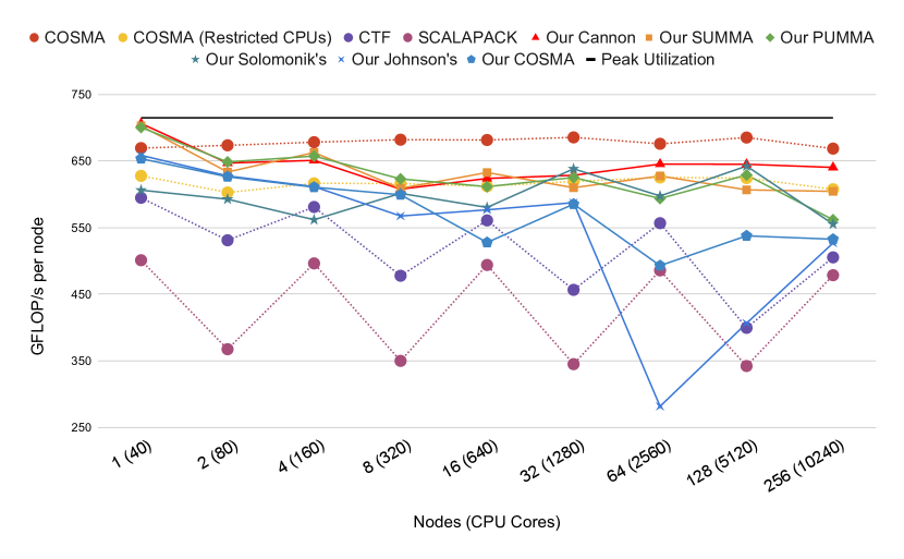
(a) CPU results.

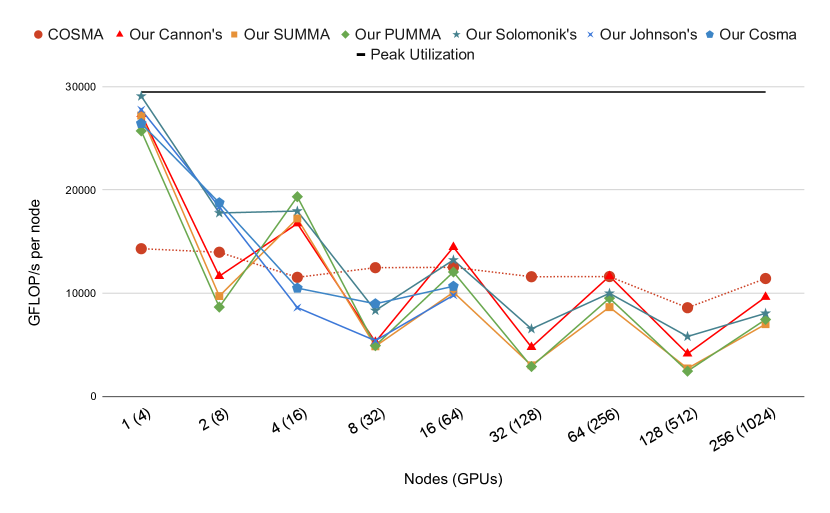
(b) GPU results.

Figure 18. Weak-scaling results (higher is better) for matrix-multiplication. DISTAL’s kernels are prefixed with ”Our” and are denoted with filled lines. Other systems (COSMA, CTF and ScaLAPACK) are denoted with dotted lines.

We evaluate DISTAL’s implementations of distributed matrix-multiplication by comparing against ScaLAPACK (Choi et al., 1992), Cyclops Tensor Framework (CTF) (Solomonik et al., 2014) and COSMA (Kwasniewski et al., 2019). ScaLAPACK is a well-known library that provides a variety of distributed kernels for many common linear algebra operations. CTF is a library for distributed tensor algebra that implements the 2.5D matrix multiplication algorithm of Solomonik et al. (Solomonik and Demmel, 2011). Finally, COSMA is recent work that provides both a theoretically optimal algorithm as well as the currently best known dense matrix-multiplication implementation. Of these systems, only COSMA has a GPU backend, so we restrict our comparison to COSMA in the GPU setting.

For comparison, we implement all algorithms discussed in Section 4, including the SUMMA algorithm used by ScaLAPACK, the 2.5D algorithm used by CTF, and the COSMA algorithm. Results for CPUs and GPUs are in Figure 18. These experiments are weak-scaled (memory per node stays constant) on square matrices, where the initial problem sizes were 8192x8192 and 20000x20000 for CPUs and GPUs respectively. Initial problem sizes were chosen to be just large enough to achieve peak utilization on a single node.

For CPUs, we find COSMA performs best with 40 ranks per node, while ScaLAPACK and CTF perform best with 4 ranks per node. For GPUs, we run COSMA with one rank per GPU. DISTAL’s kernels are run with one rank per node.

7.1.1. CPU Results

18(a) contains the CPU distributed matrix-multiplication benchmarks. At 256 nodes, CTF and ScaLAPACK achieve at most 80% performance of codes generated by our system and COSMA. They also experience performance variability due to effects from non-square machine grids. COSMA and DISTAL achieve higher performance by overlapping communication and computation more effectively—our profiles show that for CPUs, it is possible to hide nearly all communication costs with computation. Since most communication costs can be hidden, we do not find significant performance variations between the different algorithms implemented in DISTAL, except for Johnson’s algorithm, which experiences performance degradation on processor grids that aren’t perfect cubes (we model each CPU socket as an abstract DISTAL processor). Finally, we see that our best schedules are within 10% of the performance of COSMA on all node counts, and within 5% on 256 nodes. DISTAL has a penalty compared to COSMA because we allocate 4 CPU cores per node to Legion to perform runtime dependence analysis and utility work. The line named ”COSMA (Restricted CPUs)” in 18(a) shows that COSMA achieves equal performance to DISTAL when restricted to use 36 out of the 40 CPU cores, which is number of work cores allocated to DISTAL. Although use of the Legion runtime imposes a small cost (5-10%), we believe that this cost is worth paying for simpler engineering and improved programmer productivity.

7.1.2. GPU Results

18(b) contains the GPU distributed matrix-multiplication benchmarks. On a single node, all of our kernels achieve twice the performance of COSMA, and COSMA achieves 15% higher performance on 256 nodes than DISTAL’s best performing schedule. COSMA keeps all data in CPU memory and uses an out-of-core GEMM kernel that pulls data into the GPU for computation with CuBLAS. DISTAL’s kernels keep all data in GPU framebuffer memory and communicate via NVLink, achieving near-peak utilization on a single node.

In contrast to the CPU experiments, we see different performance characteristics between algorithms when moving to multiple nodes. The larger problem sizes required to achieve peak GFLOP/s on a single GPU cause the computation to be evenly balanced between communication and computation, and therefore extremely sensitive to the communication costs of each algorithm.

The 2D algorithms (Cannon, SUMMA and PUMMA) perform well at square node counts (equaling or exceeding the performance of COSMA), and perform worse at rectangular node counts, similar to the variations seen with ScaLAPACK and CTF on CPUs. This variation comes from the imbalanced communication in the rectangular case. Within the 2D algorithm family, we see that Cannon’s algorithm outperforms SUMMA and PUMMA as the node count increases. The difference is the systolic communication pattern enabled by rotate that Cannon’s algorithm uses. Avoiding the collective-style broadcasting operations and using nearest-neighbor communication only, our schedule using Cannon’s algorithm achieves higher performance at scale.

The 3D algorithms (Johnson’s, Solomonik’s 2.5D and COSMA) trade communication for extra memory use, and achieve higher performance on the non-square node counts than their 2D counterparts. Johnson’s algorithm achieves high performance when the number of GPUs is a perfect cube, but for non-cubes achieves worse performance due to over-decomposition. Our implementation of COSMA achieves better performance than Johnson’s algorithm because it can adapt the decomposition to the machine size, but does not equal the performance of the 2D algorithms due to the lack of matrix-multiplication specialized broadcast and reduction operators as in the COSMA author’s implementation. Johnson’s algorithm and our COSMA implementation run out of memory at 32 nodes, because they replicate input components onto multiple nodes, they exhaust the limited GPU memory at higher node counts. The COSMA author’s implementation use the larger CPU memory to hold matrices. Solomonik’s 2.5D algorithm interpolates between the 2D and 3D algorithms, using extra memory when possible to speed up the computation. In our implementation, we utilize extra memory on the non-square node counts, resulting in better performance than the 2D algorithms on those processor counts.

DISTAL’s kernels perform worse than COSMA and experience larger performance variations due to communication costs. Legion’s DMA system is unable to achieve peak bandwidth out of a node (18/25 GB/s) when data is resident in the GPU framebuffer memory, while the system (and COSMA) achieve near peak when data is resident in CPU memory. The Legion team plans to address this shortcoming in the future.

7.2. Higher Order Tensor Benchmarks

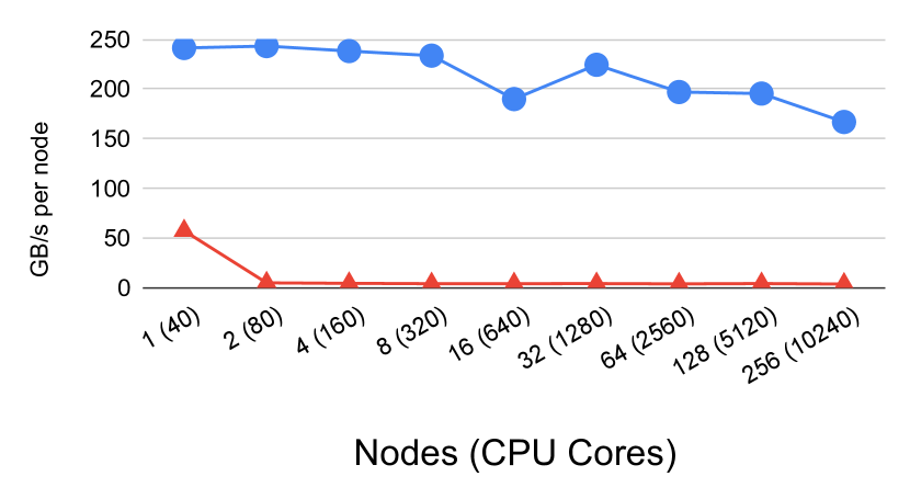
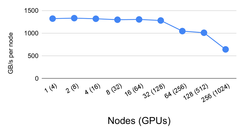
(a) TTV

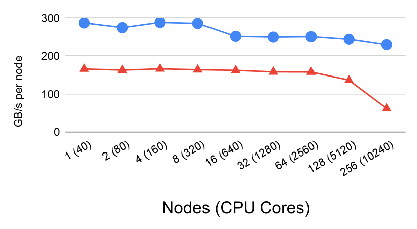
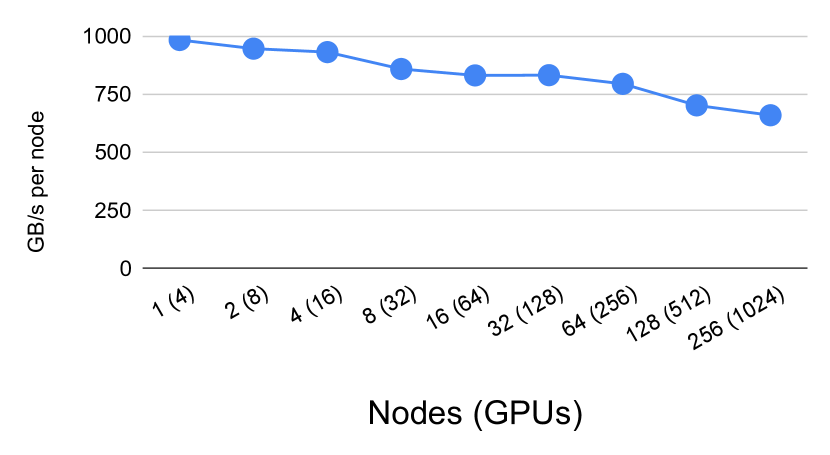
(b) Innerprod

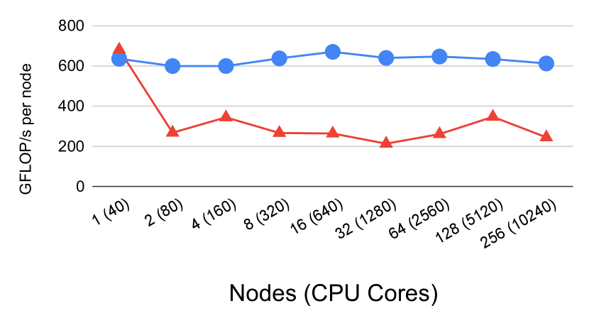
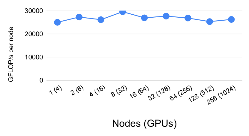
(c) TTM

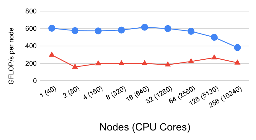
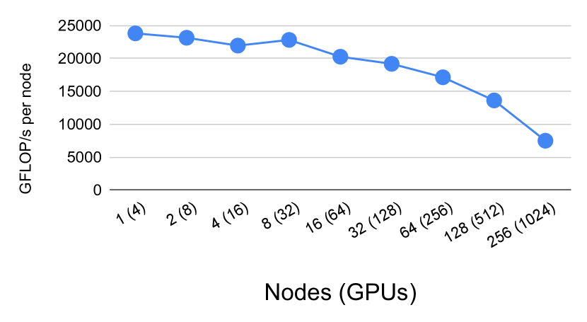
(d) MTTKRP

Figure 20. Weak-scaling results (higher is better) of higher order tensor computations.

To evaluate the generality of our system, we compare against the Cyclops Tensor Framework (CTF), which is the only system that we know of that offers similar generality: distributed implementations of any tensor algebra operation. We consider the following tensor expressions:

• Tensor times vector (TTV): $A(i,j)=B(i,j,k)\cdot c(k)$

• Inner product (Innerprod): $a=B(i,j,k)\cdot C(i,j,k)$

• Tensor times matrix (TTM): $A(i,j,l)=B(i,j,k)\cdot C(k,l)$

• Matricized tensor times Khatri-Rao Product (MTTKRP): $A(i,l)=B(i,j,k)\cdot C(j,l)\cdot D(k,l)$

These operations all have real-world applications. For example, the TTM and MTTKRP kernels are important building blocks in routines that compute Tucker and canonical polyadic decompositions of tensors (Kolda and Bader, 2009).

CTF decomposes arbitrary tensor operations into calls to a distributed matrix-multiplication implementation by slicing and reshaping the tensors. While such a strategy can implement all tensor algebra operations, it cannot implement an optimal strategy for every operation. Our approach of generating a bespoke implementation for a target kernel allows for development of a schedule that implements an optimal strategy for each kernel. Our experiments show that we outperform CTF on each higher-order tensor expression that we consider. The tradeoff between these systems is that CTF fully automates the distribution process, while users must provide a schedule to distribute their computations in DISTAL. We note that the scheduling primitives in DISTAL provide a mechanism for future work to target when automatically schedule computations for distribution.

Weak-scaling (memory per node stays constant) experiments for CPUs and GPUs are shown in Figure 20. For kernels that are bandwidth bound (TTV and innerprod), we report results in GB/s, rather than GFLOP/s. We run CTF with 4 ranks per node, for all kernels other than innerprod, where we found best performance at 40 ranks per node. Because we were unable to build CTF’s GPU backend, we only report CPU results. For each higher order kernel, we either experimented with different schedules to minimize inter-node communication (TTV, innerprod, TTM) or implemented a known algorithm (MTTKRP (Ballard et al., 2018)). Input tensors were laid out in a row-major layout and distributed in a manner that matched the chosen schedule or as specified by a proposed algorithm (MTTKRP). We used the same data distributions and distribution schedules for the CPU and GPU kernels. As with the matrix-multiplication benchmarks, initial problem sizes were chosen to be just large enough to achieve peak utilization on a single node.

7.2.1. Scheduling Leaf Kernels

Leaf kernel performance heavily impacts the overall performance of a distributed computation. To keep the leaf kernels similar between DISTAL and CTF, we use the same strategy as CTF on a single node and cast the TTM and MTTKRP operations to loops of matrix-multiplications. For element-wise operations (TTV and innerprod), we parallelize and vectorize loops for CPUs, and tile loops to thread blocks for GPUs. CTF aims at scalability to large core counts rather than fully utilizing the resources on a single node. This approach results in worse single-node performance for the TTV, innerprod and MTTKRP benchmarks (when casting MTTKRP to matrix-multiplications, an element-wise reduction operation is required).

7.2.2. Results

TTV (20(a)). Casting the TTV operation as a sequence of matrix-multiplication operations performs unnecessary communication and CTF’s performance drops past a single node. Instead, our schedule using DISTAL performs the operation element-wise without communication. Our GPU kernel achieves higher bandwidth than the CPU kernel, but starts to fall off at 256 GPUs due to the kernels’ short execution time (several milliseconds).

Innerprod (20(b)). The inner-product kernel is best implemented as a node-level reduction followed by a global reduction over all nodes, and we use this strategy in the DISTAL schedule. CTF achieves good weak scaling performance as well, but is still slower than our implementation using DISTAL. The GPU implementation of innerprod has similar performance characteristics as TTV.

TTM (20(c)). Our DISTAL schedule for TTM expresses the kernel as a set of parallel matrix-multiplication operations by distribute-ing the $i$ loop of the kernel. This strategy results in no inter-node communication and both our CPU and GPU implementations achieve high efficiency up to 256 nodes. Instead, CTF casts the kernel as a loop of distributed matrix-multiplications, which results in a large drop in performance due to inter-node communication.

MTTKRP (20(d)). DISTAL allows for implementing specialized algorithms for tensor algebra operations. We implement the algorithm of Ballard et al. (Ballard et al., 2018) that keeps the 3-tensor in place and reduces intermediate results into the output tensor. DISTAL’s kernels fall off after 64 nodes due to overheads of algorithms used within Legion to manage the situation where portions of regions are replicated onto many nodes. The Legion team plans to address this shortcoming in the future. CTF does not achieve similar performance on a single node, but has flat scaling behavior.

8. Related Work

Distributed Tensor Algebra. The only system that we know of to support distributed execution of any tensor algebra kernel is the Cyclops Tensor Framework (CTF) (Solomonik et al., 2014). CTF casts tensor contractions into a series of distributed matrix-multiplication operations and transposes, an approach also used by the single-node Tensor Contraction Engine (Baumgartner et al., 2005). Our approach of generating specialized kernel implementations can lead to improvements over CTF’s interpreted approach.

Distributed algorithms for tensor algebra have drawn interest from researchers, including the matrix-multiplication algorithms in Figure 12 and algorithms for higher order tensor algebra like MTTKRP (Ballard et al., 2018). DISTAL provides a framework to model and generate implementations for these algorithms.

Related work in the database community has taken steps to extend relational database engines to support distributed linear algebra (Luo et al., 2017) and distributed tensor computations (Jankov et al., 2021).

DSL Compilers. Several DSL compilers for single-node systems have been developed, such as Halide (Ragan-Kelley et al., 2013), TVM (Chen et al., 2018), Tensor Comprehensions (Vasilache et al., 2018), COGENT (Kim et al., 2019) and TACO (Kjolstad et al., 2017). Distributed Halide (Denniston et al., 2016) and Tiramisu (Baghdadi et al., 2018) support targeting distributed machines. Distributed Halide extends Halide with data and computation distribution commands. DISTAL supports richer data distributions (such as broadcasting and fixing tensor partitions) and targets tensor algebra instead of stencil codes. Tiramisu is a polyhedral compiler that can target distributed machines and supports scheduling commands that distribute computation and communicate data. However, these commands require more user input: users must describe the data to communicate and the processors involved. Recent work by Ihadadene (Ihadadene, 2019) automates these components for stencil codes. Unlike DISTAL, Tiramisu does not have a data distribution language or a rotate command, which limits its ability to generate some sophisticated distributed algorithms. DISTAL is the first system of this kind to separate data and computation distributions, allowing for expression of many existing distributed tensor algebra algorithms, including all of the algorithms in Figure 12.

Modeling Machines and Distributing Data. Common data distributions of arrays (such as row, column, and tiled) were first included as directives in languages for distributed programming (e.g., High Performance Fortran (Loveman, 1993)). ZPL introduced the idea of separately defining an abstract machine (e.g., as a grid of processors) and a function defining a partitioning and mapping of data onto that machine (Deitz et al., 2004). This approach has been adopted by Chapel (Chamberlain et al., 2007) and extended in Sequoia (to a hierarchical abstract machine (Fatahalian et al., 2006)) and Legion (Bauer et al., 2012) (to allowing multiple partitions of the same data or to be used simultaneously).

Dryden et al. (Dryden et al., 2019) use a similar notation as DISTAL that describes how each dimension of a tensor is distributed to describe algorithms for distributed convolutional neural network training. Dryden et al. were inspired by the FLAME (Schatz et al., 2016; Schatz, 2015) project, which used a set notation to describe tensor distributions and redistribution of tensors into different distributed layouts. DISTAL combines data distribution descriptions with a separate computation scheduling language to allow for expression of many distributed algorithms.

Distributed Polyhedral Compilation. Amarasinghe et al. (Amarasinghe and Lam, 1993) and Bondhugula (Bondhugula, 2013) used polyhedral analysis to derive communication information for computation distribution from affine loop nests statically. Our work starts from a higher level representation that allows for the expression of different algorithms through scheduling, whereas such decisions would need to be already present in the affine loops targeted by these works. The analysis of Amarasinghe et al. is fully static on a set of virtual processors, but can result in imprecise communication when mapping the virtual processors onto the physical processors. In contrast, Bondhugula generates a set of runtime calls that complement the static analysis to determine precise communication partners. The ideas presented by Bondhugula and Amarasinghe et al. could be used as analysis passes for an MPI-based backend for DISTAL and are thus orthogonal to our approach.

Discussion. The critical difference between DISTAL and prior work is the notion of specifying independently how computation and data are distributed in two high level languages. The separation of these two concepts allows for flexibility in expression of different algorithms and adaptability when integrating with existing codes—code can shape to data so that data may stay at rest. Additionally, our combined static-dynamic approach allows for expression of complex communication patterns and data distributions statically, while discharging lower level data movement operations to a runtime system. This design decision allows us to avoid complicated and, in some cases, brittle analyses used by fully static approaches.

9. Future Work

We see many interesting avenues of future work from DISTAL. One such avenue is DISTAL’s potential applications in training and evaluating distributed deep learning models, where DISTAL can be used to generate distributed kernels for stages in the model. As DISTAL allows for separation of both data and computation distribution, these parameters could be included in search-based approaches to deep learning model distribution. Another avenue is auto-scheduling and auto-formatting frameworks for DISTAL. Currently, DISTAL is a useful productivity tool allowing for application developers to develop code at a high level while performance engineers can optimize the mapping without changing application code. With automatic schedule and format selection, application developers could independently achieve high performance and allow performance engineers to optimize further when an automatic schedule is insufficient. A third avenue of future work that we are currently undertaking is to is to extend DISTAL with support for sparse tensors. The envisioned system would enable users to create distributed implementations of any desired tensor computation with any set of tensor formats.

10. Conclusion

We have introduced DISTAL, a compiler for dense tensor algebra that targets modern, heterogeneous machines. DISTAL allows for independent specifications of desired computation, data distribution, and computation distribution. The combination of data distribution and computation distribution allows for expression of widely known algorithms and optimization of higher order tensor kernels. DISTAL generates code competitive with hand-optimized implementations of matrix-multiplication and outperforms existing systems on higher order tensor kernels by between 1.8x and 3.7x.

References

- (1)
- Agarwal et al. (1995) R. C. Agarwal, S. M. Balle, F. G. Gustavson, M. Joshi, and P. Palkar. 1995. A three-dimensional approach to parallel matrix multiplication. IBM Journal of Research and Development 39, 5 (1995), 575–582. https://doi.org/10.1147/rd.395.0575
- Amarasinghe and Lam (1993) Saman Amarasinghe and Monica Lam. 1993. Communication Optimization and Code Generation for Distributed Memory Machines. Sigplan Notices - SIGPLAN 28, 126–138. https://doi.org/10.1145/173262.155102
- Baghdadi et al. (2018) Riyadh Baghdadi, Jessica Ray, Malek Ben Romdhane, Emanuele Del Sozzo, Abdurrahman Akkas, Yunming Zhang, Patricia Suriana, Shoaib Kamil, and Saman Amarasinghe. 2018. Tiramisu: A Polyhedral Compiler for Expressing Fast and Portable Code. arXiv:1804.10694 [cs.PL]
- Ballard et al. (2018) Grey Ballard, Nicholas Knight, and Kathryn Rouse. 2018. Communication Lower Bounds for Matricized Tensor Times Khatri-Rao Product. In 2018 IEEE International Parallel and Distributed Processing Symposium (IPDPS). 557–567. https://doi.org/10.1109/IPDPS.2018.00065
- Bauer et al. (2012) Michael Bauer, Sean Treichler, Elliott Slaughter, and Alex Aiken. 2012. Legion: Expressing Locality and Independence with Logical Regions. In Proceedings of the International Conference on High Performance Computing, Networking, Storage and Analysis (Salt Lake City, Utah) (SC ’12). IEEE Computer Society Press, Washington, DC, USA, Article 66, 11 pages.
- Baumgartner et al. (2005) G. Baumgartner, A. Auer, D.E. Bernholdt, A. Bibireata, V. Choppella, D. Cociorva, Xiaoyang Gao, R.J. Harrison, S. Hirata, S. Krishnamoorthy, S. Krishnan, Chi chung Lam, Qingda Lu, M. Nooijen, R.M. Pitzer, J. Ramanujam, P. Sadayappan, and A. Sibiryakov. 2005. Synthesis of High-Performance Parallel Programs for a Class of ab Initio Quantum Chemistry Models. Proc. IEEE 93, 2 (2005), 276–292. https://doi.org/10.1109/JPROC.2004.840311
- Bondhugula (2013) Uday Bondhugula. 2013. Compiling Affine Loop Nests for Distributed-Memory Parallel Architectures. In Proceedings of the International Conference on High Performance Computing, Networking, Storage and Analysis (Denver, Colorado) (SC ’13). Association for Computing Machinery, New York, NY, USA, Article 33, 12 pages. https://doi.org/10.1145/2503210.2503289
- Cannon (1969) Lynn Elliot Cannon. 1969. A Cellular Computer to Implement the Kalman Filter Algorithm. Ph.D. Dissertation. USA. AAI7010025.
- Chamberlain et al. (2007) B.L. Chamberlain, D. Callahan, and H.P. Zima. 2007. Parallel Programmability and the Chapel Language. The International Journal of High Performance Computing Applications 21, 3 (2007), 291–312. https://doi.org/10.1177/1094342007078442 arXiv:https://doi.org/10.1177/1094342007078442
- Chen et al. (2018) Tianqi Chen, Thierry Moreau, Ziheng Jiang, Lianmin Zheng, Eddie Yan, Meghan Cowan, Haichen Shen, Leyuan Wang, Yuwei Hu, Luis Ceze, Carlos Guestrin, and Arvind Krishnamurthy. 2018. TVM: An Automated End-to-End Optimizing Compiler for Deep Learning. arXiv:1802.04799 [cs.LG]
- Choi et al. (1992) J. Choi, J.J. Dongarra, R. Pozo, and D.W. Walker. 1992. ScaLAPACK: a scalable linear algebra library for distributed memory concurrent computers. In [Proceedings 1992] The Fourth Symposium on the Frontiers of Massively Parallel Computation. 120–127. https://doi.org/10.1109/FMPC.1992.234898
- Choi et al. (1994) Jaeyoung Choi, David W. Walker, and Jack J. Dongarra. 1994. Pumma: Parallel universal matrix multiplication algorithms on distributed memory concurrent computers. Concurrency: Practice and Experience 6, 7 (1994), 543–570. https://doi.org/10.1002/cpe.4330060702 arXiv:https://onlinelibrary.wiley.com/doi/pdf/10.1002/cpe.4330060702
- Deitz et al. (2004) S.J. Deitz, B.L. Chamberlain, and L. Snyder. 2004. Abstractions for dynamic data distribution. In Ninth International Workshop on High-Level Parallel Programming Models and Supportive Environments, 2004. Proceedings. 42–51. https://doi.org/10.1109/HIPS.2004.1299189
- Demmel et al. (2013) James Demmel, David Eliahu, Armando Fox, Shoaib Kamil, Benjamin Lipshitz, Oded Schwartz, and Omer Spillinger. 2013. Communication-Optimal Parallel Recursive Rectangular Matrix Multiplication. In 2013 IEEE 27th International Symposium on Parallel and Distributed Processing. 261–272. https://doi.org/10.1109/IPDPS.2013.80
- Denniston et al. (2016) Tyler Denniston, Shoaib Kamil, and Saman Amarasinghe. 2016. Distributed Halide. In Proceedings of the 21st ACM SIGPLAN Symposium on Principles and Practice of Parallel Programming (Barcelona, Spain) (PPoPP ’16). Association for Computing Machinery, New York, NY, USA, Article 5, 12 pages. https://doi.org/10.1145/2851141.2851157
- Dryden et al. (2019) Nikoli Dryden, Naoya Maruyama, Tim Moon, Tom Benson, Marc Snir, and Brian Van Essen. 2019. Channel and Filter Parallelism for Large-Scale CNN Training. In Proceedings of the International Conference for High Performance Computing, Networking, Storage and Analysis (Denver, Colorado) (SC ’19). Association for Computing Machinery, New York, NY, USA, Article 10, 20 pages. https://doi.org/10.1145/3295500.3356207
- Fatahalian et al. (2006) Kayvon Fatahalian, Daniel Reiter Horn, Timothy J. Knight, Larkhoon Leem, Mike Houston, Ji Young Park, Mattan Erez, Manman Ren, Alex Aiken, William J. Dally, and Pat Hanrahan. 2006. Sequoia: Programming the Memory Hierarchy. In Proceedings of the 2006 ACM/IEEE Conference on Supercomputing (Tampa, Florida) (SC ’06). Association for Computing Machinery, New York, NY, USA, 83–es. https://doi.org/10.1145/1188455.1188543
- Ihadadene (2019) Thinhinane Ihadadene. 2019. Generating Communication Code Automatically for Distributed Programs in Tiramisu.
- Jankov et al. (2021) Dimitrije Jankov, Binhang Yuan, Shangyu Luo, and Chris Jermaine. 2021. Distributed Numerical and Machine Learning Computations via Two-Phase Execution of Aggregated Join Trees. Proc. VLDB Endow. 14, 7 (March 2021), 1228–1240. https://doi.org/10.14778/3450980.3450991
- Kim et al. (2019) Jinsung Kim, Aravind Sukumaran-Rajam, Vineeth Thumma, Sriram Krishnamoorthy, Ajay Panyala, Louis-Noël Pouchet, Atanas Rountev, and P. Sadayappan. 2019. A Code Generator for High-Performance Tensor Contractions on GPUs. In 2019 IEEE/ACM International Symposium on Code Generation and Optimization (CGO). 85–95. https://doi.org/10.1109/CGO.2019.8661182
- Kjolstad et al. (2019) Fredrik Kjolstad, Peter Ahrens, Shoaib Kamil, and Saman Amarasinghe. 2019. Tensor Algebra Compilation with Workspaces. In 2019 IEEE/ACM International Symposium on Code Generation and Optimization (CGO). 180–192. https://doi.org/10.1109/CGO.2019.8661185
- Kjolstad et al. (2017) Fredrik Kjolstad, Shoaib Kamil, Stephen Chou, David Lugato, and Saman Amarasinghe. 2017. The Tensor Algebra Compiler. Proc. ACM Program. Lang. 1, OOPSLA, Article 77 (Oct. 2017), 29 pages. https://doi.org/10.1145/3133901
- Kolda and Bader (2009) Tamara G. Kolda and Brett W. Bader. 2009. Tensor Decompositions and Applications. SIAM Rev. 51, 3 (Aug. 2009), 455–500. https://doi.org/10.1137/07070111X
- Kwasniewski ([n.d.]) Grzegorz Kwasniewski. [n.d.]. personal communication.
- Kwasniewski et al. (2019) Grzegorz Kwasniewski, Marko Kabić, Maciej Besta, Joost VandeVondele, Raffaele Solcà, and Torsten Hoefler. 2019. Red-Blue Pebbling Revisited: Near Optimal Parallel Matrix-Matrix Multiplication. In Proceedings of the International Conference for High Performance Computing, Networking, Storage and Analysis (Denver, Colorado) (SC ’19). Association for Computing Machinery, New York, NY, USA, Article 24, 22 pages. https://doi.org/10.1145/3295500.3356181
- LLNL (2021) LLNL. 2021. Lassen. https://hpc.llnl.gov/hardware/platforms/lassen
- Loveman (1993) D.B. Loveman. 1993. High performance Fortran. IEEE Parallel Distributed Technology: Systems Applications 1, 1 (1993), 25–42. https://doi.org/10.1109/88.219857
- Luo et al. (2017) Shangyu Luo, Zekai J. Gao, Michael Gubanov, Luis L. Perez, and Christopher Jermaine. 2017. Scalable Linear Algebra on a Relational Database System. In 2017 IEEE 33rd International Conference on Data Engineering (ICDE). 523–534. https://doi.org/10.1109/ICDE.2017.108
- Ragan-Kelley et al. (2013) Jonathan Ragan-Kelley, Connelly Barnes, Andrew Adams, Sylvain Paris, Frédo Durand, and Saman Amarasinghe. 2013. Halide: A Language and Compiler for Optimizing Parallelism, Locality, and Recomputation in Image Processing Pipelines. SIGPLAN Not. 48, 6 (June 2013), 519–530. https://doi.org/10.1145/2499370.2462176
- Schatz (2015) Martin Daniel Schatz. 2015. Distributed Tensor Computations: Formalizing Distributions, Redistributions, and Algorithm Derivation. Ph.D. Dissertation. USA.
- Schatz et al. (2016) Martin D. Schatz, Robert A. Geijn, and Jack Poulson. 2016. Parallel Matrix Multiplication: A Systematic Journey. SIAM J. Sci. Comput. 38 (2016).
- Senanayake et al. (2020) Ryan Senanayake, Changwan Hong, Ziheng Wang, Amalee Wilson, Stephen Chou, Shoaib Kamil, Saman Amarasinghe, and Fredrik Kjolstad. 2020. A Sparse Iteration Space Transformation Framework for Sparse Tensor Algebra. Proc. ACM Program. Lang. 4, OOPSLA, Article 158 (Nov. 2020), 30 pages. https://doi.org/10.1145/3428226
- Solomonik and Demmel (2011) Edgar Solomonik and James Demmel. 2011. Communication-Optimal Parallel 2.5D Matrix Multiplication and LU Factorization Algorithms. In Euro-Par 2011 Parallel Processing, Emmanuel Jeannot, Raymond Namyst, and Jean Roman (Eds.). Springer Berlin Heidelberg, Berlin, Heidelberg, 90–109.
- Solomonik et al. (2014) Edgar Solomonik, Devin Matthews, Jeff R. Hammond, John F. Stanton, and James Demmel. 2014. A massively parallel tensor contraction framework for coupled-cluster computations. J. Parallel and Distrib. Comput. 74, 12 (2014), 3176–3190. https://doi.org/10.1016/j.jpdc.2014.06.002 Domain-Specific Languages and High-Level Frameworks for High-Performance Computing.
- van de Geijn and Watts (1995) Robert A. van de Geijn and Jerrell Watts. 1995. SUMMA: Scalable Universal Matrix Multiplication Algorithm. Technical Report. USA.
- Vasilache et al. (2018) Nicolas Vasilache, Oleksandr Zinenko, Theodoros Theodoridis, Priya Goyal, Zachary DeVito, William S. Moses, Sven Verdoolaege, Andrew Adams, and Albert Cohen. 2018. Tensor Comprehensions: Framework-Agnostic High-Performance Machine Learning Abstractions. arXiv:1802.04730 [cs.PL]
- Zhang et al. (2018) Yunming Zhang, Mengjiao Yang, Riyadh Baghdadi, Shoaib Kamil, Julian Shun, and Saman Amarasinghe. 2018. GraphIt: A High-Performance Graph DSL. Proc. ACM Program. Lang. 2, OOPSLA, Article 121 (Oct. 2018), 30 pages. https://doi.org/10.1145/3276491