Non-Existent Moments of Earnings Growth

Abstract

The literature often relies on moment-based measures of earnings risk, such as the variance, skewness, and kurtosis (e.g., Guvenen et al., 2019, Econometrica). However, such moments may not exist in the population under heavy-tailed distributions. We empirically show that the population kurtosis, skewness, and even variance often fail to exist for the conditional distribution of earnings growths. This evidence may invalidate the moment-based analyses in the literature. In this light, we propose conditional Pareto exponents as novel measures of earnings risk that are robust against non-existence of moments, and develop estimation and inference methods.

Using these measures with an administrative data set for the UK, the New Earnings Survey Panel Dataset (NESPD), and the US Panel Study of Income Dynamics (PSID), we quantify the tail heaviness of the conditional distributions of earnings changes given age, gender, and past earnings. Our main findings are that: 1) the aforementioned moments fail to exist; 2) earnings risk is increasing over the life cycle; 3) job stayers are more vulnerable to earnings risk, and 4) these patterns appear in both the period 2007–2008 of the great recession and the period 2015–2016 of positive growth among others.

Keywords: earnings & income risk, heavy tail, conditional Pareto exponent.

1 Introduction

One of the main goals of the literature on income dynamics is to quantify income risk. Recent studies show that the distribution of income changes has heavier tails than the normal distribution. This evidence has relevant implications for how income risk affects economic decisions. Since heavy tails incur enormous risk premium costs in economies with risk-averse agents, quantifying the tail heaviness, along with features of preferences of economic agents, is necessary to measure the social costs of the uncertainties.

However, the existing literature relies primarily on moment-based measures of income risk. For instance, the recent influential paper by Guvenen, Karahan, Ozkan, and Song (2019) uses skewness and kurtosis to characterize the distributions of individual earnings dynamics in the U.S and provide their policy implications. They target this set of moments in their proposed procedure to estimate the parameters of a flexible stochastic process of earnings. The estimated process further feeds back into economic research and policy analyses, for instance in the analysis of life-cycle incomplete market models. While sample skewness and sample kurtosis are generally finite, their true population counterparts may not exist when the distribution has a heavy tail. If the population moments do not exist, then their sample counterparts do not make sense.

In this paper, we address this issue by first proposing a method of estimation and inference about the conditional Pareto exponent, which characterizes the tail heaviness. Second and more importantly, applying our method to the administrative data set for the UK, the New Earnings Survey Panel Dataset (NESPD), and the US Panel Study of Income Dynamics (PSID), we quantify the tail heaviness in the distribution of earnings changes and discuss how it varies with heterogeneous attributes of individuals. We find that the commonly used measures of income risk, such as sample kurtosis, skewness, and even standard deviation, may be misleading since their population counterparts may not exist (i.e., may be infinite) for the conditional distribution of earnings growth given age, gender, and past earnings. Finally, by interpreting the conditional Pareto exponent as a robust measure of the conditional earnings risk, we show that tail earnings risk increases over the life cycle, is higher for job-stayers, and these patterns appear in both the period 2007–2008 of the great recession and the period 2015–2016 of a positive growth despite some differences.

There is an extensive literature on earnings and income dynamics models, dating back to the 1970s – see the comprehensive survey by Moffitt and Zhang (2018). To explain the heavy tail feature, the existing literature exploits the following strategies: 1) fitting data to mixed normal distributions using mixture approaches (Geweke and Keane, 2000; Bonhomme and Robin, 2009); 2) conducting nonparametric density estimates and graphically exhibiting heavier tails than normal distributions with deconvolution and spectral decomposition approaches (Horowitz and Markatou, 1996; Bonhomme and Robin, 2010; Arellano, Blundell, and Bonhomme, 2017; Botosaru and Sasaki, 2018; Hu, Moffitt, and Sasaki, 2019); 3) reporting the sample moments such as skewness and kurtosis and comparing them with counterparts from normal distribution (Guvenen, Karahan, Ozkan, and Song, 2019; Arellano, Bonhomme, De Vera, Hospido, and Wei, 2021, among others); 4) reporting some quantile-based measures such as Kelly’s measure of skewness and Crow-Siddiqui measure of kurtosis (Guvenen, Karahan, Ozkan, and Song, 2019, among others); and 5) reporting the mean absolute deviation (Arellano, Bonhomme, De Vera, Hospido, and Wei, 2021).

The first approach, based on mixed normal distribution, essentially assumes an exponentially decaying tail, which cannot characterize tail heaviness. The second one is based on nonparametric density estimation, which tends to behave poorly in the tails due to few extreme observations. The third approach based on sample moments may yield misleading information if the population moment does not exist due to heavy tails. In particular, the population kurtosis may not exist even if a researcher can always get a finite sample kurtosis. We indeed find that the population kurtosis, skewness, and even variance may not exist. The fourth one is robust to heavy tails: these non-extremal quantile-based measures are always well-defined even if the population moments do not exist. However, they fail to capture extreme income changes and tail events. Among other things, information on tail events is central to quantifying earnings risk under heavy-tailed distributions. Like the fourth one, the fifth approach based on the first moment alone is not informative about extreme income changes and tail events.

Given the above concerns about existing approaches, we aim for an alternative measure of tail heaviness to characterize the earnings risk conditional on individuals’ attributes. The conditional Pareto exponent is proposed as our robust measure of tail heaviness. We have the elegant characterization that the conditional kurtosis/skewness/variance is infinite if and only if the conditional Pareto exponent is smaller than the value of four/three/two. We propose methods of estimation and inference about the Pareto exponent in the conditional distribution of earnings risk given observed attributes, such as gender, age, and base-year income level. Unlike the aforementioned approaches, this new method can be used to characterize the tail heaviness robustly even if the rate of tail decay is slower than exponential ones and even if the population kurtosis, skewness, or variance is infinite.

To illustrate the empirical significance, we apply the proposed method to two data sets: the UK NESPD and the US PSID, with our focus on the former. NESPD is an employer-based survey data set on individual earnings in the UK and has been investigated very recently (cf. De Nardi, Fella, and Paz-Pardo, 2021; Bell, Bloom, and Blundell, 2021). We contribute to this new literature with the following three findings. First, we find that the distribution of the earnings changes (measured by the difference between the log earnings across two subsequent years) conditional on age, gender, and past earnings exhibits substantially heavy tails. The conditional Pareto exponent is significantly less than four for the majority of the subpopulations, raising the concern that the kurtosis may be infinite. Also, the conditional Pareto exponent is significantly less than three or even two for some subpopulations, and we thus reject the hypothesis of finite conditional skewness and even finite conditional variance. These results are robust across years, including the period of recession in 2007-2008 and the period of positive growth in 2015-2016 among others.

Second, we find remarkable patterns that the tail earnings risk is increasing over the life cycle. This is documented as that 40- and 50-year-old workers face higher earnings risk than 30-year-old workers. Third, we quantify the tail heaviness of the distribution of earnings changes for job-stayers and find that, at low earnings levels, conditional kurtosis does not exist, contrary to what we observe for the whole population. Excluding middle-aged men at top quantiles of earnings, we reject the hypothesis of finite conditional kurtosis for job-stayers at all earnings levels. In Appendix C, we also apply our method to the US PSID and obtain similar empirical findings on the tail heaviness of the conditional distribution of income risk.

The above findings closely compare to the finding in Guvenen, Karahan, Ozkan, and Song (2019) and the income literature inspired by their methodology. In particular, Guvenen, Karahan, Ozkan, and Song (2019) find in the US data set that the conditional variance of earnings risk is higher for younger workers at the bottom of the income distribution, and the kurtosis increases with age and with lagged income up to the top 5% of the income distribution where it sharply declines. Since the data exhibit substantially heavier tails than those of the normal distribution, these sample moments could be less informative if their population counterparts are indeed infinite. Our results confirm theirs, but now with our new measure of earnings risk robust to infinite moments. On the other hand, our findings differ from those in Arellano, Bonhomme, De Vera, Hospido, and Wei (2021), who examine the Spanish administrative data, and find that the income risk measured by the conditional mean absolute deviations is inversely related to income and age, and the income risk inequality increases markedly in the recession. The differences can be explained by a number of factors, such as different countries and different sample selection criteria as well as different measures of income risk for different research objects.

Organization: The rest of the paper is organized as follows. Section 2 describes the data to be examined in this article and provides some descriptive analysis of the heavy-tail phenomena in the earnings growth risk. Section 3 formally introduces our econometric method, and Section 4 applies it to the UK data set. Section 5 concludes with some remarks. The Appendix collects asymptotic theories, computational details, Monte Carlo simulations, additional empirical results with the UK and US data sets, and mathematical proofs.

2 Data and Preview

2.1 New Earnings Survey Panel Data

We start with introducing the New Earnings Survey Panel Data (NESPD), an administrative data set at the individual level on UK earnings from the UK Social Security. It is an annual panel running from 1975 to 2016, and it surveys around 1% of the UK workforce. All employees whose National Insurance Number (NIN) ends in a given pair of digits are included in the survey. The NIN number is randomly issued to all UK residents at age 16 and kept constant throughout the lifetime of an individual. The NESPD is a survey directed to all employers whose employees qualify for the sample: the employers complete the questionnaire based on payroll records for their employees. As a result of being directed to the employer, NESPD has a low non-classical measurement error.

The survey reports the employees’ gender, age, and detailed work-related information: annual, weekly, and hourly earnings, hours of work, occupation, industry, working area, firms’ number of employers, and unionization. This information relates to a specified week in April of each year: the data sample is taken on the first day of April of each calendar year and concerns complete employee records only. The NESPD contains complete information on the employees’ working life from the first year they started working (or 1975 if later) until retirement age (or 2015 if earlier), as long as the employer answered the questionnaire and the individual was working with the last recorded employer in April.

Given that NESPD contains detailed information on earnings and a long panel component, it has been used for a broad range of topics in the literature: among the others, Goos and Manning (2007) have used NESPD to document job polarization in the UK; Nickell and Quintini (2003) and Elsby et al. (2016) have employed this study for analysis of wage rigidities; Adam et al. (2019) provide an analysis of valid response rates in NESDP. However, the study of income and earnings dynamics in the UK has not received lots of attention, with a couple of notable exceptions in recent years: De Nardi et al. (2021) and Bell et al. (2021) are two main references for earnings dynamics in the UK using NESPD for the analysis.

The information in NESPD is of exceptionally high quality. However, it is worth mentioning that not all workers are covered and there are non-negligible non-response issues. In particular, data in NESPD are collected in a specified week of April. As a result, NESPD might under-sample part-time workers if their weekly earnings fall below the threshold for paying National Insurance and those that moved jobs recently. Furthermore, the data set is unbalanced with possibly non-random missing observations. This issue might be problematic for representativeness of those at the bottom of the distribution and with unstable spells. We refer to Bell et al. (2021) and De Nardi et al. (2021) for a deeper investigation of the data limitations of NESPD.

Following the earnings literature, we further extract a subset of NESPD, which correspond to employees with a strong attachment to the labor force. Specifically, we follow De Nardi et al. (2021) to use the following selection criteria: we drop the observations below 5% of the median earnings (roughly £1,300 a year), individuals whose total working hours exceed 80 hours per week, and individuals that display negative values in earnings or hourly wages; we do not consider individuals whose hours worked or weekly pay are missing. Earnings are deflated using CPI (2015=100). The earnings measure is the residual obtained by regressing the logarithm of earnings on year and age dummies. We extract a portion of data for a pair of years across the period of the great recession, 2007-2008. The above-described sample selection leaves 78,531 individuals.

For the purpose of comparisons, we also use the portion of data for the pair, 2015 and 2016, of the most recent survey years. Note that this period is associated with positive economic growth in the UK. The sample selection procedure described above leaves 95,906 individuals for this period. The results for other years are similar and hence postponed to Appendix B for readability.

Apart from age, gender, and income, we could further consider industry and occupation as heterogeneous attributes in the analysis. NESPD contains information on both industry and occupation with the Standard Industry Classification (SIC) and Standard Occupation Classification (SOC) codes.

We define a measure $Y$ as the difference between the log earnings in 2007 and the log earnings in 2008 (i.e., one-year earnings growth rate). Similarly, we also construct this variable for the period between 2015 and 2016. Figures 1 and 2 show the kernel density estimates of the measure $Y$ for the period 2007–2008 and the period 2015–2016, respectively. In each figure, the top and bottom panels show the densities for men and women, respectively. The figures illustrate clear departures from normality: each kernel density exhibits a large spike in the middle of the distribution sticking upward out of the reference normal density. Moreover, each kernel density has heavier tails compared to the reference normal density. These features of the estimated densities suggest that the actual distributions of $Y$ indeed have heavier tails than normal distributions, as documented in the previous literature.

We also inspect the sample moments of the distribution of one-year earnings changes conditional on previous earnings. Figure 3 shows the standard deviation, the Kelly’s measure of skewness, and the Crow-Siddiqui measure of kurtosis, respectively, of earnings changes by previous earnings, for men (left three figures) and women (right three figures). The Kelly’s measure of skewness is defined as $(Q_{.9}Y-Q_{.5}Y)-(Q_{.5}Y-Q_{.1}Y)/(Q_{.9}Y-Q_{.1}Y)$ and the Crow-Siddiqui measure of kurtosis as $(Q_{.975}Y-Q_{.025}Y)/(Q_{.75}Y-Q_{.25}Y)$, where $Q_{\tau}Y$ denotes the $\tau$-quantile of the distribution of $Y$. As in De Nardi et al. (2021), we find that the Crow-Siddiqui measure of kurtosis is higher than the reference value of 2.91 for the normal distribution, and the Kelly’s measure of skewness deviates from zero, ranging from positive values for low earnings groups to negative values for higher values of previous earnings. However, as mentioned in the introduction, these quantile-based measures do not take into account the very tail observations that are above, say $Q_{.975}Y$. These observations are indeed informative about the tail feature of the earnings risk and inequality. In comparison, our proposed method takes all samples into consideration and is explicitly designed to characterize the tail heaviness.

In the rest of the paper, we analyze the heaviness of the tails of the conditional distributions of $Y$ given the earnings level and age in the base year (i.e., the base year is 2007 for the period 2007–2008 and it is 2015 for the period 2015–2016). Specifically, the heaviness of the tails is quantified by the conditional Pareto exponent, and we propose an econometric method of estimation and inference about this measure of tail heaviness. Its value, in particular, informs whether the $r$-th conditional moments of the income growth exist for $r=2,3,4$, and so on. If the conditional Pareto exponent, $\alpha(x_{0})$, given $X=x_{0}$ is less than $r$, then the conditional distribution of $Y$ given $X=x_{0}$ does not have a finite $r$-th moment. Section 3 introduces a method of estimation and inference, and Section 4 presents the empirical results. It turns out that we reject the hypotheses of finite conditional kurtosis, finite conditional skewness, and even finite conditional standard deviation for some subpopulations.

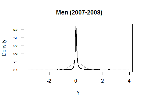
Figure 1: Kernel density estimates (black line) of $Y$, which is defined as a one-year change in log earnings, in 2007 in the NESPD. The left (respectively, right) panel shows the density of men (respectively, women). Also shown in gray dashed lines are the normal density fit to data. Number of individuals: 38,955 men (39,576 women).

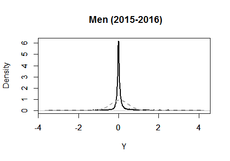
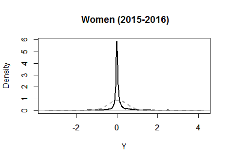
Figure 2: Kernel density estimates (black line) of $Y$, which is defined as a one-year change in log earnings, in 2015 in the NESPD. The left (respectively, right) panel shows the density of men (respectively, women). Also shown in gray dashed lines are the normal density fit to data. Number of individuals: 45,985 men (49,921 women).

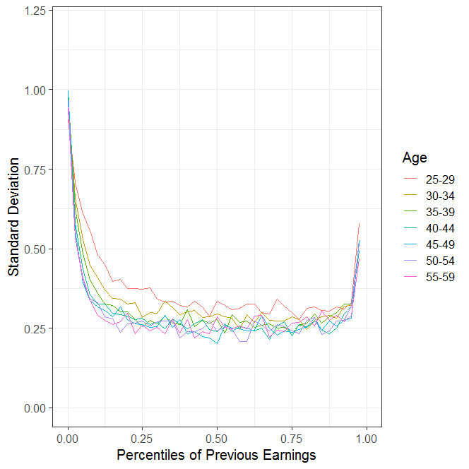
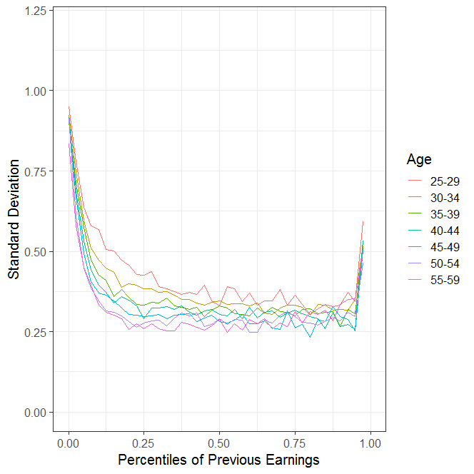
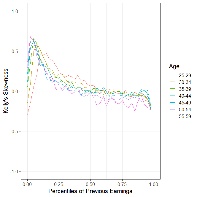
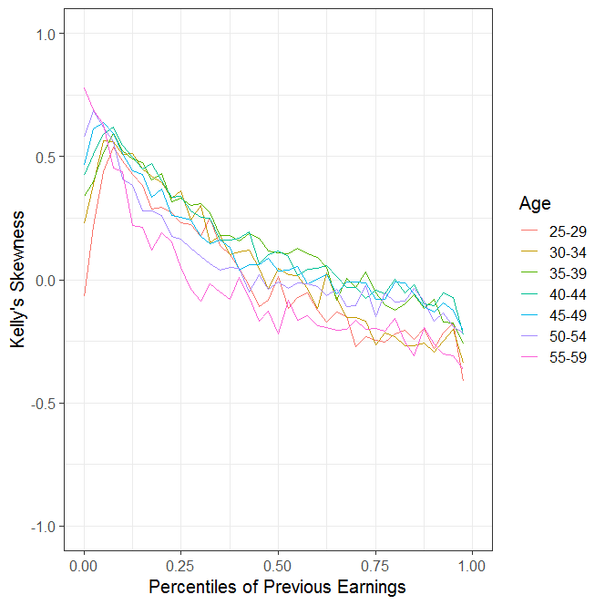
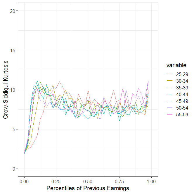
Figure 3: Moments of one-year log earnings changes by previous earnings, for men (left) and women (right) based on the NESPD.

3 Measurement of Conditional Tail Risk

We now introduce our proposed measure of conditional tail risk, and present method of estimation and inference. Formal theoretical justifications are relegated to the appendix. Let $Y$ denote the variable of interest and let $X$ denote a vector of individual characteristics, such as the income level and age in the base year. Assume that the sample is i.i.d. so that the joint distribution $F_{Y,X}\left(\cdot,\cdot\right)$ of $(Y,X)$ is unique. In this section, we present an econometric method to study tail features (e.g., existence of the variance, skewness, kurtosis, and so on) of the conditional distribution $F_{Y|X=x_{0}}$ of $Y$ given $X=x_{0}$ for pre-specified values $x_{0}$ of the individual characteristics $X$.

Consider a rectangular array $\{(Y_{ij},X_{ij}):i\in\{1,\cdots,I\},j\in\{1,\cdots,J\}\}$. Such a data structure can be constructed by randomly splitting a cross-sectional data set of size $N$ into an $I\times J$ array such that $I\cdot J\approx N$, which is what we implement in Section 4. See Appendix A.3 for how to choose $I$ and $J$ in practice under such a construction of an array.

Assume that the conditional distribution $F_{Y|X=x_{0}}\left(\cdot\right)$ is regularly varying at infinity, that is,

$$1-F_{Y|X=x_{0}}(y)\propto y^{-\alpha(x_{0})}\mathcal{\ }\text{as }y\rightarrow\infty\text{,}$$

where $\alpha\left(x_{0}\right)>0$ denotes the $x_{0}$-conditional Pareto exponent that characterizes the tail heaviness of the conditional distribution of $Y$ given $X=x_{0}$. We note that this Pareto-type tail condition is mild and satisfied by many commonly used distributions, such as Student-t, F, and gamma distributions. Moreover, it has been widely documented that the earnings data set exhibits a Pareto-type tail and hence supports this condition (cf. Gabaix, 2009, 2016; Guvenen, Karahan, Ozkan, and Song, 2019). See Appendix A.1 for more discussions and primitive conditions.

With the parameter $\alpha\left(x_{0}\right)$, we can characterize the existence of the conditional moments as follows. For any $r\in\mathbb{R}^{+}$,

$$\mathbb{E}\left[Y_{ij}^{r}|X_{ij}=x_{0}\right]< \infty\text{ if }\alpha(x_{0})>r\qquad\text{and}$$

$$\mathbb{E}\left[Y_{ij}^{r}|X_{ij}=x_{0}\right]= \infty\text{ if }\alpha(x_{0})<r.$$

Thus, the test of finite conditional $r$-th moment can be represented by the competing hypotheses

$$H_{0}:\alpha(x_{0})>r\text{ against }H_{1}:\alpha(x_{0})\leq r.$$ (1)

In particular, we set $r=2$, $3$, and $4$ for tests of the existence of the standard deviation, skewness, and kurtosis, respectively.

To construct a feasible test for (1), we need to obtain a random sample from the conditional distribution $F_{Y|X=x_{0}}\left(\cdot\right)$. This would be straightforward if $X$ is discrete. However, random sampling from such a conditional distribution is infeasible when $X$ includes at least one continuous random variable, such as the income level, which we use in our data analysis. To overcome this issue, we propose the following procedure to extract the local sample. Let $\left|\left|\cdot\right|\right|$ denote the Euclidean norm.

1. For each $i$, find the nearest neighbor (NN) of $\{X_{ij}\}_{j=1}^{J}$ to $x_{0}$ and the induced $Y_{ij}$ associated with the NN, that is $Y_{ij}=Y_{ij^{\ast}}$ where $\left|\left|X_{ij^{\ast}}-x_{0}\right|\right|=\min_{j\in\{1,...,J\}}\left|\left|X_{ij}-x_{0}\right|\right|$. Denote the induced $Y$ by $\{Y_{i,[x_{0}]}\}_{i=1}^{I}$.

2. Sort $\{Y_{i,[x_{0}]}\}_{i=1}^{I}$ descendingly as $\{Y_{(1),[x_{0}]}\geq Y_{(2),[x_{0}]}\geq,...,\geq Y_{(n),[x_{0}]}\}$. Collect the largest $K+1$ of them as

   $$\mathbf{Y}(x_{0})=\{Y_{(1),[x_{0}]},Y_{(2),[x_{0}]},...,Y_{(K+1),[x_{0}]}\}.$$

3. Use $\mathbf{Y(}x_{0}\mathbf{)}$ to estimate the Pareto exponent $\alpha\left(x_{0}\right)$ by the formla in (2) below.

We postpone until Appendix A.1 formal discussions of conditions under which this procedure works and why it works in theory. Here, we instead discuss its intuition. First, for each $i$, we select the NN among $\{X_{ij}\}_{j=1}^{J}$ to $x_{0}$. When $J$ (as well as $I$) is large enough, such a NN gets close enough to $x_{0}$ and therefore its induced value $Y_{i,[x_{0}]}$ behaves as if it were generated from $F_{Y|X=x_{0}}$. Second, given the i.i.d. assumption, the subsample $\{Y_{i,[x_{0}]}\}_{i=1}^{I}$ collected from all individuals serves as a random sample approximately generated from $F_{Y|X=x_{0}}$. We can thus use the extreme order statistics of $\{Y_{i,[x_{0}]}\}_{i=1}^{I}$ to estimate the Pareto exponent $\alpha\left(x_{0}\right)$ by using one of the many existing methods. In particular, if we apply the estimator of Hill (1975) to this NN sample $\{Y_{i,[x_{0}]}\}_{i=1}^{I}$, then we get an estimator

$$\hat{\alpha}(x_{0})=\left[\frac{1}{K}\sum_{k=1}^{K}\{\log(Y_{(k),[x_{0}]})-\log\left(Y_{(K+1),[x_{0}]}\right)\}\right]^{-1},$$ (2)

of the conditional Pareto exponent $\alpha(x_{0})$. See Appendix A.3 for how to choose $K$ in practice.

We show in Appendix A.1 that this estimator asymptotically follows the normal distribution as

$$\sqrt{K}\left(\hat{\alpha}(x_{0})-\alpha(x_{0})\right)\overset{d}{\rightarrow}\mathcal{N}\left(0,\alpha(x_{0})^{2}\right)$$ (3)

under suitable conditions. Moreover, for any $x_{0}\neq x_{1}$, we also have the joint asymptotic normality:

$$\sqrt{K}\binom{\hat{\alpha}(x_{0})-\alpha(x_{0})}{\hat{\alpha}(x_{1})-\alpha(x_{1})}\overset{d}{\rightarrow}\mathcal{N}\left(0,\left(\begin{array}[]{cc}\alpha(x_{0})^{2}&0\\ 0&\alpha(x_{1})^{2}\end{array}\right)\right).$$ (4)

We provide a formal statement of these results as Proposition 1 in Appendix A.1.

Given (3) and (4), we can construct the standard t and F tests for our hypothesis testing problem (1). Specifically, we reject the (one-sided) null hypothesis at the 5% nominal level if

$$\frac{\hat{\alpha}(x_{0})-r}{\sqrt{K}\hat{\alpha}(x_{0})}<\Phi^{-1}(0.05),$$ (5)

where $\Phi^{-1}\left(\cdot\right)$ denotes the quantile function of the standard normal distribution and $r=2$, $3$, and $4$. Moreover, we reject the null hypothesis that $\alpha(x_{0})=\alpha(x_{1})$ (against the two-sided alternative) at the 5% nominal level if

$$\frac{\left|\hat{\alpha}(x_{0})-\hat{\alpha}(x_{1})\right|}{\sqrt{K}\sqrt{\hat{\alpha}(x_{0})^{2}+\hat{\alpha}(x_{1})^{2}}}>\Phi^{-1}(1-0.025).$$ (6)

Appendix A.2 contains a simulation study, which supports our theoretical results.

We end this section with discussions about the related econometrics and statistics literature. To estimate the unconditional Pareto exponent of some underlying distribution, researchers have developed numerous methods, including the popular and widely used Hill’s (1975) estimator, and those proposed by Smith (1987) and Gabaix and Ibragimov (2011). We refer to de Haan and Ferreira (2007) for a comprehensive review. In recent work, Beare and Toda (2017) show that the cumulative sum of Markov multiplicative processes generates an approximate Pareto tail. This result supports our theoretical conditions and fits our empirical setup.

Unlike the unconditional Pareto exponent of, say $Y$, estimating its conditional counterpart given some other variable $X$ has received less attention. This is technically more challenging when $X$ contains continuous random variables as one could not obtain a random sample from the conditional distribution of interest, say $F_{Y|X=x_{0}}$ for some pre-specified value $x_{0}$. Wang and Tsai (2009) and Wang and Li (2013) impose some parametric assumptions such that the Pareto exponent is a single index function of $X$. Gardes and Girard (2008) and Gardes et al. (2012) develop fully nonparametric methods based on local smoothing. Estimation and inference based on these local smoothing methods sensitively rely on the bandwidth parameter unlike our proposed method based on nearest neighbors. Furthermore, these existing methods underperform compared to ours in terms of bias and standard deviation, as demonstrated through simulation studies presented in Appendix A.2. For these reasons, we suggest using our novel method proposed above.

Finally, in two related papers, Trapani (2016) and Degiannakis et al. (2022) propose randomized testing procedures to test the finiteness of moments of a random variable or the residual of the linear regression. Unlike their proposal, we test the existence of moments of the conditional distribution of a random variable given some other variables. To see the difference, consider, for example, the model that $Y=\mu(X)+\sigma(X)U$ where $\mu(X)$ and $\sigma(X)$ are some functions of $X$ that characterize the location and scale of $Y$ respectively. One can estimate these two functions and further estimates the tail heaviness of $Y$ by that of the residual $\hat{U}$. But such a model by construction assumes that the tail heaviness of $Y$ remains unchanged across $X$ (cf. Wang and Li, 2013). This feature is neither sufficient for our purpose of measuring the tail heaviness of earnings growth as a function of demographic characteristics nor coherent with the empirical findings. Also related is the paper by Sasaki and Wang (2022), who propose inference for the tail index of conditional distributions. Although allowing the tail index to depend on $X$, their inference method builds on the fixed-$k$ asymptotics and cannot be easily extended for estimation. In our context, estimation is valuable and thereby, we can propose a novel measure of earnings risk based on the estimate of the tail index unlike any of these existing papers. As such, our proposal is suitable for studying the tail features of the conditional distribution of income growth and relates these to the results in the income literature.

4 Results

4.1 Benchmark Sample

Applying the method introduced in Section 3 (and also in more detail in Appendix A) to NESPD described in Section 2.1, we analyze the conditional tail risk of earnings of adult individuals in the United Kingdom. We define $Y$ by the absolute difference of the log earnings in 2007 and the log earnings in 2008 for our baseline analysis. For the conditioning variables $X$, we include the quantile of earnings level and the age of the individual in the base year (2007), following Guvenen et al. (2019). With this setting, we study the conditional Pareto exponent $\alpha(x_{0})$ for each point $x_{0}$ of earnings levels from $\{0.05,0.10,\cdots,0.90,0.95\}$ (in quantile) and ages from $\{30,40,50\}$ for each of men and women.

Figure 4 illustrates the estimates of the conditional Pareto exponents $\alpha(x_{0})$ (in black lines) along with the upper bounds of their one-sided 95% confidence intervals (in gray lines) for 30-, 40- and 50-year-old individuals. The left (respectively, right) panel shows the results for men (respectively, women) in each figure, which suggests different patterns of heterogeneous earnings risk across age, base-year earnings, and gender groups.

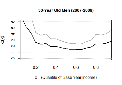
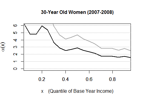
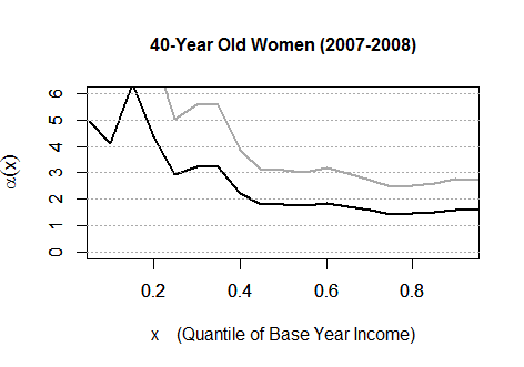
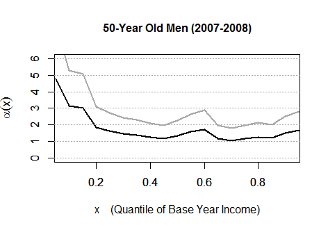
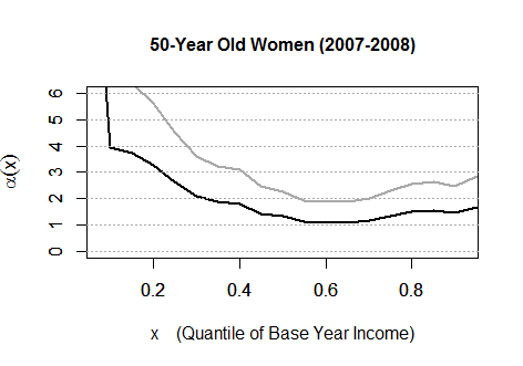
Figure 4: Estimates (black lines) and the one-sided 95% confidence intervals (gray lines) of the Pareto exponents $\alpha(x_{0})$ of the conditional tail risk for men (left) and women (right) based on the NESPD in the period 2007–2008. The left (respectively, right) column shows the results for men (respectively, women). The top, middle, and bottom panels show the results for 30-, 40- and 50-year-old individuals.

We describe the empirical findings in the order of age and gender. For 30-year-old men (the top left panel in Figure 4), the conditional Pareto exponents (in point estimates) range from 1.4 to 7.0, and the upper bounds of the one-sided 95% confidence intervals range from 2.3 to 11.4. Given any quantile of earnings received in 2007, with the exception of the very top and bottom quantiles, the conditional Pareto exponent is significantly less than four, implying that the conditional kurtosis of earnings growth does not exist for these middle-earnings groups of young men. Overall, the kurtosis barely exists for most of the base-year earnings levels even if we fail to reject the hypothesis of finite kurtosis. Furthermore, given that earnings received in 2007 were between the 45th and the 75th percentile, the Pareto exponent is significantly less than three, implying that even the conditional skewness does not exist. For 30-year-old women (the top right panel in Figure 4), the conditional Pareto exponents (in point estimates) range from 1.5 to 6.1, and the upper bounds of the one-sided 95% confidence intervals range from 2.5 to 10.0. For this subpopulation, the conditional Pareto exponent is significantly less than four for high- and middle-high-earnings groups of women, those above the 60th percentile of the earnings distribution in 2007, implying that the conditional kurtosis does not exist. Furthermore, given that earnings received in 2007 were at or above the 70th percentile, the Pareto exponent is significantly less than three, implying that even the conditional skewness does not exist. Comparing the results between men and women at age 30, we observe that women were more vulnerable to earnings risk than men at the top quantiles of the base-year income level, above the 75th percentile.

For 40-year-old men (the middle left panel in Figure 4), the conditional Pareto exponents (in point estimates) range from 1.2 to 9.1, and the upper bounds of the one-sided 95% confidence intervals range from 1.9 to 14.9. Remarkably, the earnings risks of 40-year-old men are higher than those of 30-year-old men. For this age group of men, we reject the hypothesis of finite kurtosis at any level of base-year earnings, apart from the bottom quantiles, below the 15th percentile. Furthermore, given that earnings received in 2007 were between the 20th and the 35th percentile and above or at median excluding the very top quantile (between the 75th and 80th percentile), the Pareto exponent is significantly less than three (two), implying that even the conditional skewness (respectively, standard deviation) does not exist. For 40-year-old women (the middle right panel in Figure 4), the conditional Pareto exponents (in point estimates) range from 1.4 to 6.4, and the upper bounds of the one-sided 95% confidence intervals range from 2.4 to 11.0. For this age group of women, we reject the hypothesis of finite kurtosis at any earnings level above the 40th percentile. Furthermore, given that earnings received in 2007 were at or above the 65th percentile, the Pareto exponent is significantly less than three, implying that even the conditional skewness does not exist. Comparing the results between men and women at age 40, we observe that men are almost as vulnerable to earnings risk as women for this middle age group, with some difference at the bottom quantiles.

For 50-year-old men (the bottom left panel in Figure 4), the conditional Pareto exponents (in point estimates) range from 1.1 to 4.8, and the upper bounds of the one-sided 95% confidence intervals range from 1.8 to 8.0. For this age group of men, we reject the hypothesis of finite kurtosis and finite skewness at any level of base-year earnings, apart from the bottom quantiles, below the 20th percentile. Moreover, we reject the hypothesis of finite standard deviation at the 45th percentile and between the 65th and the 75th percentile. For 50-year-old women (the bottom right panel in Figure 4), the estimated conditional Pareto exponents range from 1.1 to 15.0, and the upper bounds of the one-sided 95% confidence intervals range from 1.9 to 25.7. For this age group of women, we reject the hypothesis of finite kurtosis at any level of base-year earnings, apart from the bottom quantiles, below the 30th percentile. Moreover, we reject the hypothesis of finite skewness (standard deviation) at any level of base-year earnings above the 40th percentile (between the 55th and the 70th percentile).

4.2 Period of Positive Growth

While our main focus has been on the period of great recession between 2007 and 2008, we next look at the period of positive growth, between 2015 and 2016. Figure 5 illustrates the results for earnings growth between 2015 and 2016 for 30-, 40- and 50-year-old individuals. These results share similar qualitative patterns to those reported in Figure 4. First, 30-year-old men at high quantiles of base-year earnings enjoy less earnings risk. Second, 40-year-old men have an overall higher earnings risk than 30-year-old men. Lastly, and most remarkably, for men the earnings risk is not necessarily lower in the period 2015–2016 than in the period 2007–2008, even though the former period enjoyed a positive GDP growth (2.2% in 2015 and 1.8% in 2016) and the latter period suffered from negative GDP growth (0.7% in 2007 and $-$4.4% in 2008). Women, instead, are less vulnerable to earnings risk in the period 2015–2016 than in the period 2007–2008. Overall, there are more similarities than differences despite the contrast between a recession and a positive growth in the UK economy.

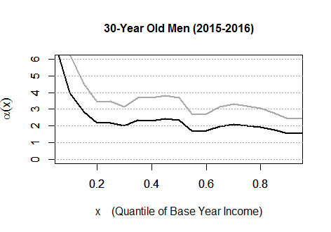
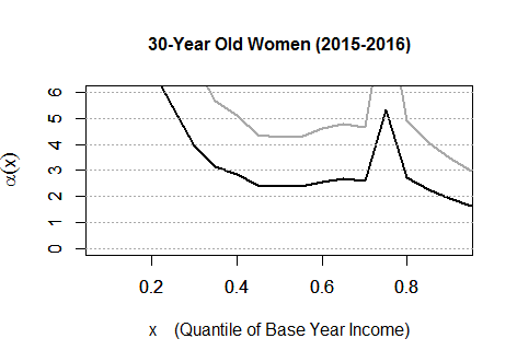
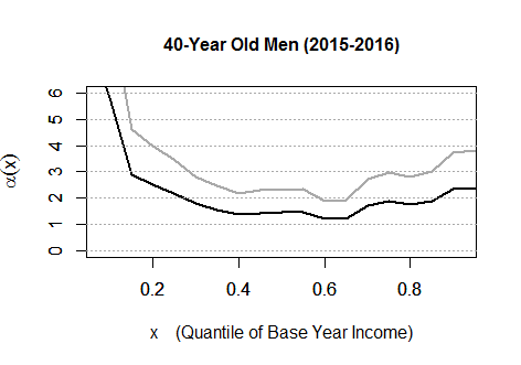
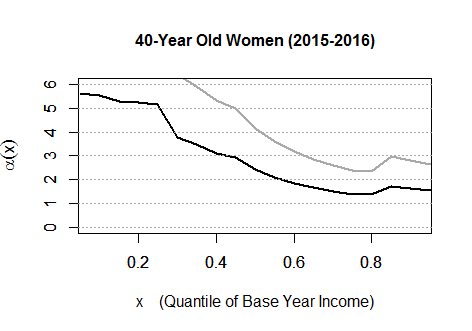
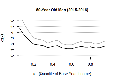
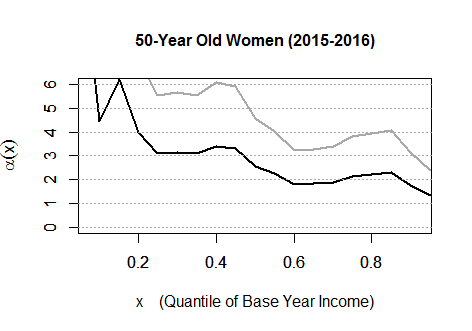
Figure 5: Estimates (black lines) and the one-sided 95% confidence intervals (gray lines) of the Pareto exponents $\alpha(x_{0})$ of the conditional tail risk for men (left) and women (right) based on the NESPD in the period 2015–2016. The left (respectively, right) column shows the results for men (respectively, women). The top, middle, and bottom panels show results for 30-, 40- and 50-year-old individuals.

In summary, we find that: 1) the kurtosis, skewness, and even standard deviation may not exist for the conditional distribution of earnings growth given certain attributes (age, gender, and earnings); 2) 40- and 50-year-old workers have overall higher earnings risk than 30-year-old workers and we thus document that tail earnings risk is increasing over the life cycle; and 3) these patterns appear both in the period 2007–2008 of great recession and the period 2015–2016 of a positive growth for men, while there are some differences for women. Finally, we remark that, although we use the two periods, 2007–2008 and 2015–2016, to draw the above conclusion, we also present additional empirical results for other periods between 2005 and 2016 in Appendix B to demonstrate a robustness. In Appendix C, we also apply our proposed method to the US PSID and obtain similar empirical findings on the tail heaviness of the conditional distribution of income risk.

4.3 Job Stayers

We also experiment with a different set of selection criteria: we restrict the sample to workers who did not change their jobs in the last twelve months. We refer to them as job stayers. Figures 6 and 7 illustrate estimates of the conditional Pareto exponents $\alpha(x_{0})$ (in black lines) along with the upper bounds of their one-sided 95% confidence intervals (in gray lines) for the two pairs of years: 2007–2008 and 2015–2016, with the restricted sample of job stayers. Figures 6 and 7 show that, for almost all attributes, conditional kurtosis does not exist at any level of baseline earnings.

This finding is in line with the US evidence documented by Guvenen et al. (2019) that job stayers experience different earnings dynamics and, in particular, face earnings innovations that are more leptokurtic, especially at the bottom of the earnings distribution.

More specifically, we find that, at low earnings levels, conditional kurtosis does not exist, in contrast to what we observe for the whole population. Excluding middle-aged men at top quantiles of earnings, we reject the hypothesis of finite conditional kurtosis for job-stayers at all earnings levels.

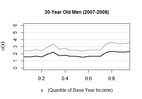
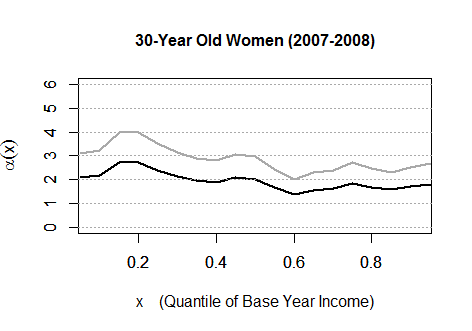
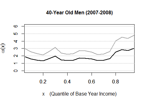
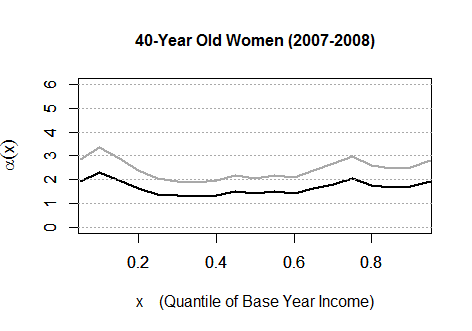
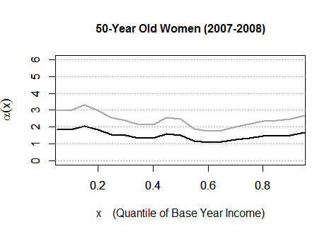
Figure 6: Estimates (black lines) and the one-sided 95% confidence intervals (gray lines) of the Pareto exponents $\alpha(x_{0})$ of the conditional tail risk for men (left) and women (right) based on the NESPD in the period 2007–2008, for job-stayers. The left (respectively, right) column shows the results for men (respectively, women). The top, middle, and bottom panels show results for 30-, 40- and 50-year-old individuals. Number of individuals: 32,411 men (32,509 women).

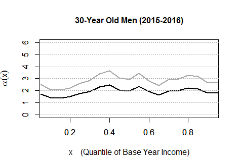
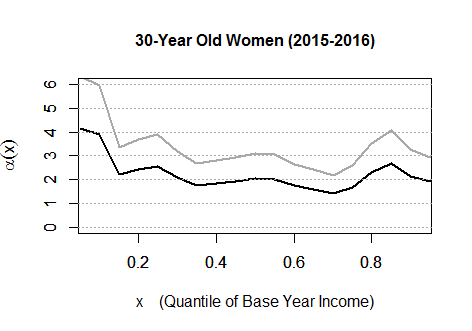
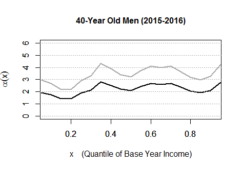
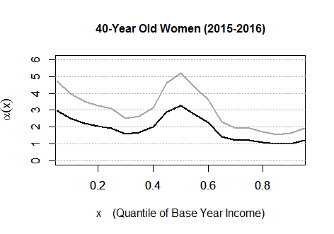
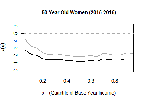
Figure 7: Estimates (black lines) and the one-sided 95% confidence intervals (gray lines) of the Pareto exponents $\alpha(x_{0})$ of the conditional tail risk for men (left) and women (right) based on the NESPD in the period 2015–2016, for job-stayers. The left (respectively, right) column shows the results for men (respectively, women). The top, middle, and bottom panels show results for 30-, 40- and 50-year-old individuals. Number of individuals: 38,680 men (41,393 women).

4.4 Discussion

Our findings confirm that moment-based measures, such as variance, skewness, or kurtosis, may not be well-defined for some sub-populations. This result points to the importance of using alternatives to the moment-based measures of earnings risk typically used in the literature. We propose a measure of conditional tail earnings risk that overcomes this limitation and offers new insights into the amount of tail risk. Our measure quantifies the amount of risk related to, possibly extreme, shocks individuals experience, given their lagged income and age profile.

Our first finding is that, compared to younger, older individuals are more likely to be hit by potentially large shocks, e.g., health shocks or occupation changes. For the US, Guvenen et al. (2019) document that earnings growth of males aged 45-55 and earning $100,000 has a kurtosis of 18, compared to 5 for younger workers earning $10,000 (and 3 for a Gaussian distribution). These findings highlight the importance of life cycle effects in tail earnings risk, but these estimates are unreliable since kurtosis might not exist in the first place. Our methodology allows measuring this conditional tail risk and indeed reveals that older workers are much more vulnerable to extreme shocks (estimates of our measure are close to 1 along a large part of the distribution of lagged earnings) compared to younger individuals (for which our estimates are close to 2 or larger). Similarly, in our second finding, we show that job stayers face earnings shocks that are more leptokurtic, especially at the bottom of the earnings distribution (at the bottom of the earnings distribution, estimates of our measure go from 5 for the whole sample to around 1 for job stayers). In addition, the frequency and occurrence of leptokurtic shocks do not seem to differ in recessions. A further investigation of the nature of these shocks might shed more light in this direction. To sum up, our results for the whole sample demonstrate that tail earnings risk increases over the life cycle and is higher for job stayers than for movers. Moreover, at least for the male subsample, there are no relevant differences between recession and expansion periods in our proposed measure of tail earnings risk.

It is worth discussing how our methodology and results differ from those of other papers in the literature on earnings risks. Guvenen et al. (2019), among others, use moment-based measures, which we have shown to be not well-defined, and complement the analysis with quantile-based measures. Although well-defined when moments may fail to exist, quantile-based measures do not capture extreme events since they do not include observations larger or smaller than some given percentiles. Given our interest in conditional tail earnings risk, the excluded tail observations contain valuable information for the analysis. Among other things, information on tail events is central to quantifying earnings risk under heavy-tailed distributions. Thus, the quantile-based approach may not be informative about extreme income changes and tail events.

Another measure proposed in the literature is the coefficient of variation (CV) of Arellano et al. (2021), computed as the ratio between the mean absolute deviation of income divided by the mean income, conditional on a set of variables. Estimating the numerator and denominator of the CV are two prediction tasks performed with Poisson regressions with both micro and macro predictors. The main idea is to capture the agent’s prediction problem by focusing on features of the predictive distribution of income. One of their main findings is that younger individuals face higher levels of income risk, and the dispersion of the CV markedly increases in recessions. These results contrast what we obtain with our measure of conditional tail risk. In order to understand what drives the differences between our results and their findings, we build the CV measure of earnings risk with NESPD for the UK to separate the country and institutional effect from the differences due to the different methodology and object of interest. Indeed, the divergences could reflect differences in terms of institutional context, sample selection, and the types of measures used to quantify income risk. There are several constraints in replicating their approach due to some data limitations. For instance, in our case, earnings are the only source of income as we do not observe unemployment benefits. We thus capture a less broad measure of risk compared to theirs. Acknowledging these data limitations, we computed the CV for UK workers. We get qualitatively similar findings to those in Arellano et al. (2021), although the magnitude of the coefficient of variation is different. In particular, we get a smaller dispersion of the CV compared to what they report for Spain. As in their case, however, we obtain that younger individuals face higher risk: for this subgroup, the coefficient of variation is higher, with the 90th percentile of their CV being much larger than the corresponding CV percentile for other age groups. Thus, institutional settings, different sample sizes, and datasets matter for the magnitude of the results, not for the qualitative differences. We can conclude that the main differences between our findings and theirs come from the different concepts of risk we are measuring rather than differences in context (Spain vs. the UK in this particular case). As with quantile-based measures in Guvenen et al. (2019), also with the CV measure proposed by Arellano et al. (2021), one might fail to capture extreme income changes and tail events. Our measure captures a different aspect of earnings risk: it quantifies tail risk, and thus, it should be seen as complimentary to their proposal.

Finally, in our baseline analysis, we define $Y$ as the absolute value of log earnings changes. We repeat the analysis separately for the left and the right tail of the distribution of earnings changes. For the left and right tails separately considered, the estimates of the Pareto exponent are always not significantly smaller than 4, and point estimates can get much higher values (up to 50 for the right tail, for some subpopulations). Overall, the patterns of the left and right tails resemble those of the absolute changes tail. However, despite these similarities, there are some remarkable differences, especially at the bottom and top of the earnings distribution. More specifically, for the left tail, estimates tend to be lower (taking a maximum value of around 11) and relatively constant or decreasing over the earnings quantiles. Instead, for the right tail, estimates are much more variable and lower at the bottom of the earnings distribution. This finding is consistent with the patterns of asymmetry of conditional Kelley’s skewness documented in figure 3: higher earners are more likely to face large negative earnings shocks, because of limited opportunities for large gains and higher risk of significant declines, while the vice versa holds for workers at the bottom of the earnings distribution.

5 Concluding Remarks

The literature often relies on moment-based measures of earnings risk, such as the variance, skewness, and kurtosis, but such moments may not exist in population under heavy-tailed distributions. In this paper, we show that the population kurtosis, skewness, and even variance indeed often fail to exist for the conditional distribution of earnings growths given age, gender, and past earnigs. Hence, moment-based analyses in the literature may not make sense under heavy-taied distributions.

Heavy tails of income and earnings risk distributions are costly in economies with risk-averse agents. Despite this common knowledge, the tail heaviness has been arguably less investigated in the literature on earnings and income dynamics. In light of the limited capacity of moment-based measures in quantifying the tail-heaviness, we consider the conditional Pareto exponent as a novel robust measure of conditional earnings risk given observed attributes of individuals and propose a method of estimation and inference about this measure.

Applying the proposed method to the UK NESPD and, in Appendix, to the US PSID, we obtain the following findings. First, as emphasized above, the population kurtosis, skewness, and even standard deviation might be infinite for the conditional distribution of income growth given certain attributes, such as age, gender, and lagged income, and, hence, their sample counterparts might be less informative. Second, 40- and 50-year-old workers have overall higher earnings risk than 30-year-old workers, thus earnings risk increases over the life cycle. Third, conditional earnings risk is higher for job stayers, in particular, at the bottom of the earnings distribution. Fourth, these patterns appear both in the period of great recession and the period of a positive growth, while there are differences as well, especially for women.

To the best of our knowledge, this is the first work to shed light on tail features of heavy-tailed distributions of earnings and income growth with a formal econometric method. While we focused on two specific data sets for empirical analysis, we hope that our proposed method will spur further empirical research with other data sets and for the study of other economies.

Appendix

Appendix A provides additional details about the econometric method introduced in Section 3. Appendix B provides additional empirical results with the UK NESPD. Appendix C provides the results with the US PSID.

Appendix A Additional Details about Section 3

Appendix A.1 presents a formal statement of the asymptotic normality results, (3) and (4). Appendix A.2 presents simulation studies. Appendix A.3 suggests a choice of $I$, $J$, and $K$ and a finite sample adjustment in practice.

A.1 Econometric Theory

In this appendix section, we provide a formal statement of the asymptotic normality results, (3) and (4). We consider the following conditions to establish these results.

Condition 1

1. $(Y_{ij},X_{ij}^{\intercal})^{\intercal}$ is i.i.d. across $i$ and $j$. In addition, $f_{X}\left(x\right)$ is uniformly continuously differentiable and bounded away from zero in an open ball centered at $x_{0}$.

2. $1-F_{Y|X=x}(y)=c(x)y^{-\alpha(x)}\left(1+d(x)y^{-\gamma(x)}+r(x,y)\right)$ uniformly as $y\rightarrow\infty$ where $c(\cdot)>0$ and $d(\cdot)$ are continuously differentiable functions and uniformly bounded between $0$ and $\infty$, $\alpha(\cdot)>0$ and $\gamma\left(\cdot\right)>0$ are continuously differentiable functions and $r(x,y)$ is continuously differentiable with bounded derivatives w.r.t. both $x$ and $y$ and satisfies $\lim\sup_{y\rightarrow\infty}\sup_{x\in B_{\delta}(x_{0})}\left|r(x,y)/y^{-\gamma(x)}\right|=0$ for some open ball $B_{\delta}(x_{0})$ centered at $x_{0}$ with radius $\delta>0$.

3. $K=o\left(n^{2\gamma(x_{0})/\left(\alpha(x_{0})+2\gamma(x_{0})\right)}\right)\rightarrow 0$ as $n\rightarrow\infty$.

4. $I\rightarrow\infty$ and $\lim_{I\rightarrow\infty}J/I^{\lambda}=C\in\left(0,\infty\right)$ for some $C$ and $\lambda\in\left(0,\infty\right)$. In addition, $\lambda/2\geq\gamma(x_{0})/(\alpha(x_{0})+2\gamma(x_{0}))$.

Condition 1.1 requires the data to be independent across $i$ and $j$. Condition 1.2 assumes that the target conditional distribution satisfies a second-order Pareto tail approximation. The parameter $\gamma(x)$ governs the preciseness of the Pareto tail approximation, and the approximation error $r(x,y)$ is asymptotically negligible. The unconditional version (i.e., without $x$) of this condition has been commonly imposed in the statistics literature. Essentially, this Pareto-type tail condition is satisfied by all distributions whose densities are smooth and monotonically decay to zero, as referred to the von Mises’ condition. See de Haan and Ferreira (2007) for a comprehensive review.

Condition 1.3 specifies the choice of $K$, a tuning parameter that characterizes the number of larger order statistics to be considered as stemming from the tail. Such a choice is to eliminate the asymptotic bias. If we choose $K$ such that $K\times n^{-2\gamma(x_{0})/\left(\alpha(x_{0})+2\gamma(x_{0})\right)}\rightarrow\mu(x_{0})$ for some constant $\mu(x_{0})\in\mathbb{R}$, then the asymptotic distribution in Proposition 1 involves one additional item $-\mu(x_{0})\xi(x_{0})$. To avoid such bias, we can select a smaller order $K$ as in Condition 1.3 such that $\mu(x_{0})$ becomes zero asymptotically. This is close in spirit to choosing the undersmoothing bandwidth in the standard kernel estimation. Condition 1.4 requires a large $I$ and a large $J$. Note that $J$ can be substantially smaller than $I$ when $\lambda$ is less than one.

The following proposition characterizes the asymptotic behavior of $\hat{\alpha}\left(x_{0}\right)$ given in (2) under Condition 1.

Proposition 1

Suppose that Condition 1 holds. Then

$$\sqrt{K}\left(\hat{\alpha}(x_{0})-\alpha(x_{0})\right)\overset{d}{\rightarrow}\mathcal{N}\left(0,\alpha(x_{0})^{2}\right).$$

Moreover, for any $x_{0}\neq x_{1}$, $\hat{\alpha}(x_{0})$ and $\hat{\alpha}(x_{1})$ are asymptotically independent, or equivalently,

$$\sqrt{K}\binom{\hat{\alpha}(x_{0})-\alpha(x_{0})}{\hat{\alpha}(x_{1})-\alpha(x_{1})}\overset{d}{\rightarrow}\mathcal{N}\left(0,\left(\begin{array}[]{cc}\alpha(x_{0})^{2}&0\\ 0&\alpha(x_{1})^{2}\end{array}\right)\right).$$

Proof.

For convenience of writing, we also introduce the notation $\xi(x_{0})=1/\alpha(x_{0})$, which is referred to as the tail index. We estimate $\hat{\xi}\left(x_{0}\right)$ by the reciprocal of $\hat{\alpha}(x_{0})$, that is,

$$\hat{\xi}(x_{0})=\frac{1}{K}\sum_{k=1}^{K}\{\log(Y_{(k),[x_{0}]})-\log\left(Y_{(K+1),[x_{0}]}\right)\}.$$

Using similar lines of arguments to the proof of Theorem 2 in Sasaki and Wang (2022), we have that

$$\sqrt{K}\left(\hat{\xi}(x_{s})-\xi(x_{s})\right)\overset{d}{\rightarrow}\mathcal{N}\left(0,\xi(x_{s})^{2}\right)$$ (7)

for $s=1,0$. In particular, we use $\alpha(x_{0})$ and $\gamma(x_{0})$ to denote their $\gamma(x_{0})$ and $\tilde{\gamma}\left(x_{0}\right)$, respectively. Besides, their asymptotic bias term $\mu_{H}$ becomes zero by our Condition 1.3. Thus, the asymptotic distribution of $\hat{\alpha}\left(x_{s}\right)$ for $s=1,0$ is derived by the delta method.

Now, it remains to show the asymptotic independence between $\hat{\xi}(x_{1})$ and $\hat{\xi}(x_{0})$ for any $x_{1}\neq x_{0}$. Given their joint asymptotic Gaussianity, it suffices to show that

$$K\cdot\text{Cov}\left[\hat{\xi}(x_{1})-\xi(x_{1}),\hat{\xi}(x_{0})-\xi(x_{0})\right]\rightarrow 0,$$

which is proved as follows.

First, given the i.i.d. condition across $i$, we have that

$$\text{Cov}\left[\log(Y_{i_{1},[x_{0}]}),\log(Y_{i_{2},[x_{1}]})\right]=0\text{ for any }i_{1}\neq i_{2}.$$ (8)

Moreover, given the i.i.d. condition across $j$, the standard argument in the induced order statistics literature (e.g., Lemma 3.1 in Bhattacharya (1984)) yields that, for any $i$, conditional on $\mathbf{X}_{i}\equiv\{X_{i,1},...,X_{i,J}\}$, the induced order statistics $\{Y_{i,(1)},...,Y_{i,(J)}\}$ are independent. Denote $X_{i,[x]}$ as the NN of $\{X_{i,j}\}_{j=1}^{J}$ to $x$. Therefore as long as $X_{i,[x_{0}]}\neq X_{i,[x_{1}]}$, we have that

$$\text{Cov}\left[\log(Y_{i,[x_{0}]}),\log(Y_{i,[x_{1}]})\right]$$ (9)

$$= \mathbb{E}\left[\text{Cov}\left[\log(Y_{i,[x_{0}]}),\log(Y_{i,[x_{1}]})|X_{i,1},...,X_{i,J}\right]|\mathbf{X}_{i}\right]$$

$$= \mathbb{E}\left[\text{Cov}\left[\log(Y_{i,j_{0}}),\log(Y_{i,j_{1}})|X_{i,j_{0}}=X_{i,[x_{0}]},X_{i,j_{1}}=X_{i,[x_{1}]}\right]|\mathbf{X}_{i}\right]$$

$$= 0$$

by the law of iterated expectations. Since $X_{ij}$ contains at least one continuous component, Lemma 1 in Sasaki and Wang (2022) implies that $\left|\left|X_{i,[x_{0}]}-x_{0}\right|\right|=o_{a.s.}(1)$ and $\left|\left|X_{i,[x_{1}]}-x_{1}\right|\right|=o_{a.s.}\left(1\right)$ as $J\rightarrow\infty$. This yields that, for any $i$,

$$\mathbb{P}\left[X_{i,[x_{0}]}=X_{i,[x_{1}]}\right]=o(1)\text{ as }J\rightarrow\infty.$$ (10)

Now, recall that $\hat{\xi}(x_{1})=K^{-1}\sum_{i=1}^{K}\{\log(Y_{(i),[x_{1}]})-\log\left(Y_{(K+1),[x_{1}]}\right)\}$, which involves $\{Y_{i_{1},[x_{1}]},...,Y_{i_{K+1},[x_{1}]}\}$ for some indices $i_{1},...,i_{K+1}\in\{1,...,I\}$. Symmetrically, we have that $\hat{\xi}(x_{0})=K^{-1}\sum_{i=1}^{K}\{\log(Y_{(i),[x_{0}]})-\log\left(Y_{(K+1),[x_{0}]}\right)\}$, which involves $\{Y_{i_{1}^{\prime},[x_{1}]},...,Y_{i_{K+1}^{\prime},[x_{1}]}\}$ for some indices $i_{1}^{\prime},...,i_{K+1}^{\prime}\in\{1,...,I\}$. By (8), the only potentially non-zero components in $\text{Cov}[\hat{\xi}(x_{1}),\hat{\xi}\left(x_{0}\right)]$ will be $\text{Cov}\left[\log(Y_{i,[x_{1}]}),\log(Y_{i,[x_{0}]})\right]$ for $i\in$ $\{i_{1},...,i_{K+1}\}\cap\{i_{1}^{\prime},...,i_{K+1}^{\prime}\}$. However, these terms are still zero by (9) if $X_{i,[x_{0}]}\neq X_{i,[x_{1}]}$, which happens with probability approaching one by (10). This completes a proof of the proposition. ∎

A.2 Simulation Analysis

In this section, we present simulation studies of finite sample performance of the proposed estimation and inference method. In each iteration, we randomly generate an $I\times J$ array $\{Y_{ij},X_{ij}\}$ according to the following two designs. Design 1: $Y_{ij}\sim\text{Pareto}(\alpha(X_{ij}))$ where $\alpha(x)=1+10x$ and $X_{ij}\sim\text{Uniform}(0,1).$ Design 2: $Y_{ij}\sim\text{Pareto}(\alpha(X_{ij}))$ where $\alpha(x)=10*(x^{2}-x+1)$ and $X_{ij}\sim\text{Uniform}(0,1).$ We estimate $\alpha(x_{0})$ by $\hat{\alpha}(x_{0})$ for each of $x_{0}\in\{0.1,0.2,\cdots,0.8,0.9\}$. Each set of Monte Carlo simulations consists of 1000 iterations of this process.

Tables 1 and 2 report the results across various values of $I=J\in\{500,1000\}$ and $K\in\{10,20\}$ under Design 1 and Design 2, respectively. Displayed statistics are the bias (Bias), standard deviation (SD), root mean square error (RMSE), and 95% coverage frequency (95% Cover). Observe that the RMSE shrinks as $K$ increases. Furthermore, the 95% coverage frequencies are close to the nominal probability. These results demonstrate desired finite sample performance of the proposed method of estimation and inference.

$I=J=500$	$x_{0}$
$K=10$	0.100	0.200	0.300	0.400	0.500	0.600	0.700	0.800	0.900
Bias	0.221	0.304	0.497	0.594	0.614	0.712	0.979	0.920	1.069
SD	0.759	1.125	1.476	2.043	2.178	2.812	3.066	3.608	4.002
RMSE	0.791	1.166	1.558	2.128	2.263	2.901	3.219	3.724	4.142
95% Cover	0.948	0.957	0.963	0.952	0.963	0.952	0.956	0.950	0.949
$I=J=500$	$x_{0}$
$K=20$	0.100	0.200	0.300	0.400	0.500	0.600	0.700	0.800	0.900
Bias	0.121	0.158	0.207	0.273	0.262	0.370	0.519	0.451	0.519
SD	0.512	0.722	0.951	1.287	1.448	1.773	2.126	2.141	2.568
RMSE	0.526	0.740	0.973	1.316	1.472	1.811	2.189	2.188	2.620
95% Cover	0.949	0.966	0.956	0.937	0.959	0.947	0.945	0.954	0.943
$I=J=1000$	$x_{0}$
$K=10$	0.100	0.200	0.300	0.400	0.500	0.600	0.700	0.800	0.900
Bias	0.244	0.333	0.580	0.574	0.643	0.861	0.813	0.981	1.205
SD	0.815	1.233	1.589	1.996	2.357	2.780	2.947	3.287	3.809
RMSE	0.851	1.277	1.692	2.077	2.443	2.910	3.057	3.431	3.995
95% Cover	0.957	0.951	0.963	0.953	0.956	0.947	0.954	0.962	0.965
$I=J=1000$	$x_{0}$
$K=20$	0.100	0.200	0.300	0.400	0.500	0.600	0.700	0.800	0.900
Bias	0.122	0.148	0.272	0.254	0.315	0.432	0.418	0.459	0.471
SD	0.508	0.767	1.007	1.219	1.453	1.760	2.020	2.183	2.537
RMSE	0.523	0.781	1.043	1.245	1.487	1.812	2.063	2.231	2.580
95% Cover	0.944	0.950	0.957	0.947	0.958	0.946	0.953	0.965	0.947

Table 1: Simulation results under Design 1.

$I=J=500$	$x_{0}$
$K=10$	0.100	0.200	0.300	0.400	0.500	0.600	0.700	0.800	0.900
Bias	1.020	0.921	0.989	0.967	0.872	0.702	0.856	0.986	1.000
SD	3.483	3.164	3.060	2.895	2.957	2.922	3.083	3.332	3.689
RMSE	3.629	3.295	3.216	3.052	3.083	3.005	3.200	3.475	3.822
95% Cover	0.957	0.960	0.963	0.955	0.948	0.950	0.951	0.965	0.953
$I=J=500$	$x_{0}$
$K=20$	0.100	0.200	0.300	0.400	0.500	0.600	0.700	0.800	0.900
Bias	0.523	0.408	0.448	0.514	0.375	0.335	0.397	0.576	0.527
SD	2.266	2.026	1.979	1.881	1.822	1.784	1.887	2.105	2.252
RMSE	2.325	2.066	2.030	1.950	1.860	1.815	1.929	2.183	2.313
95% Cover	0.958	0.951	0.936	0.948	0.956	0.947	0.953	0.953	0.953
$I=J=1000$	$x_{0}$
$K=10$	0.100	0.200	0.300	0.400	0.500	0.600	0.700	0.800	0.900
Bias	0.843	0.933	0.944	0.765	0.725	0.824	0.790	0.750	1.131
SD	3.409	3.349	3.015	2.795	2.890	3.063	2.891	3.344	3.586
RMSE	3.512	3.476	3.160	2.897	2.979	3.172	2.997	3.428	3.760
95% Cover	0.951	0.961	0.970	0.956	0.952	0.950	0.965	0.951	0.951
$I=J=1000$	$x_{0}$
$K=20$	0.100	0.200	0.300	0.400	0.500	0.600	0.700	0.800	0.900
Bias	0.474	0.401	0.446	0.359	0.339	0.413	0.440	0.324	0.495
SD	2.256	2.130	2.069	1.831	1.910	1.962	1.913	2.033	2.299
RMSE	2.306	2.168	2.116	1.866	1.940	2.005	1.963	2.059	2.352
95% Cover	0.953	0.948	0.944	0.947	0.947	0.948	0.960	0.947	0.941

Table 2: Simulation results under Design 2.

For comparison, we also implement the fully nonparametric method proposed by Gardes and Girard (2008). In particular, given a random sample of $(Y_{i},X_{i})$ of size $N$ and a pre-determined bandwidth $b$, we follow Gardes and Girard (2008) to select all the observations that satisfy $|X_{i}-x_{0}|\leq b$, where $x_{0}$ again denotes the conditional value. Given this selected subsample, we sort the $Y_{i}$’s and construct the standard Hill estimator based on the largest $K+1$ order statistics as in (2). Since there is no theoretical justification of the choice of $b$, we implement various values of $b\in\{0.01,0.025,0.05,0.075,0.1,0.125,0.15,0.175,0.2\}$ for sensitivity check. We generate data from Design 1 described above and set $x_{0}=0.5$. The sample size is $N=I*J\in\{500^{2},1000^{2}\}$. Table 3 presents the results with 1000 iterations. We summarize the findings as follows. First, the choice of bandwidth has a substantial effect on the performance of this nonparametric estimator. The bias is small only when the bandwidth is within a narrow window, which theoretically depends on the unknown higher-order parameters. Second, compared with Table 1, this nonparametric estimator has larger bias and standard deviations than our proposed method when the bandwidth is small enough to guarantee the correct coverage.

$N=500^{2}$	$b$
$K=10$	0.010	0.025	0.050	0.075	0.100	0.125	0.150	0.175	0.200
Bias	0.627	0.562	0.479	0.428	0.296	-0.064	-0.360	-0.549	-0.994
SD	2.349	2.238	2.213	2.186	2.153	2.068	2.058	1.952	1.849
RMSE	2.430	2.307	2.263	2.227	2.172	2.068	2.088	2.026	2.098
95% Cover	0.956	0.947	0.946	0.947	0.933	0.902	0.867	0.856	0.763
$N=500^{2}$	$b$
$K=20$	0.010	0.025	0.050	0.075	0.100	0.125	0.150	0.175	0.200
Bias	0.284	0.334	0.118	0.086	-0.106	-0.383	-0.654	-0.916	-1.269
SD	1.482	1.549	1.453	1.501	1.444	1.359	1.196	1.184	1.086
RMSE	1.509	1.584	1.457	1.503	1.448	1.411	1.362	1.496	1.670
95% Cover	0.952	0.950	0.937	0.937	0.927	0.881	0.852	0.770	0.656
$N=1000^{2}$	$b$
$K=10$	0.010	0.025	0.050	0.075	0.100	0.125	0.150	0.175	0.200
Bias	0.842	0.501	0.457	0.294	0.088	-0.238	-0.565	-0.804	-1.024
SD	2.488	2.283	2.249	2.200	2.128	2.112	2.037	1.842	1.780
RMSE	2.625	2.336	2.294	2.219	2.129	2.124	2.113	2.009	2.053
95% Cover	0.966	0.951	0.950	0.933	0.921	0.891	0.828	0.806	0.758
$N=1000^{2}$	$b$
$K=20$	0.010	0.025	0.050	0.075	0.100	0.125	0.150	0.175	0.200
Bias	0.360	0.350	0.143	0.022	-0.219	-0.449	-0.713	-1.015	-1.360
SD	1.490	1.507	1.410	1.428	1.447	1.346	1.321	1.170	1.089
RMSE	1.532	1.546	1.416	1.428	1.463	1.418	1.501	1.548	1.742
95% Cover	0.961	0.958	0.947	0.930	0.892	0.869	0.807	0.747	0.631

Table 3: Simulation results of the nonparametric estimator under Design 1.

A.3 Choice of $I$, $J$, and $K$

In this appendix section, we present a rule of choosing $I$, $J$, and $K$ in practice when a random sample of size $N$ is available. For simplicity, we consider the Pareto distribution family as a reference. In this case, we have $\gamma(x_{0})=\infty$ in Condition 1, and hence $\lambda\geq 1$. Since $K$ is the effective sample size in the asymptotic normality result and $K$ in turn increasing in $I$, the goal is to choose $\lambda\geq 1$ such that $I$ is large. By Condition 1.4, such a choice is $\lambda=1$. We therefore suggest to set $I=J=\sqrt{N}$.

Once $I$ has been chosen, then we can choose $K$ by adapting the diagnostic method proposed by Guillou and Hall (2001). We consider the case of estimating $\alpha(x_{0})$ here. Define $Z_{i}=i\log(Y_{(i),[x_{0}]}/Y_{(i+1),[x_{0}]})$ for $i=1,\ldots,I$. Suppose that $Y_{i,[x_{0}]}$ is exactly Pareto distributed with exponent $\alpha(x_{0})=:1/\xi(x_{0})$. Then, $Z_{i}$ should be i.i.d. with the exponential distribution and satisfies $\mathbb{E}\left[Z_{i}\right]=\xi(x_{0})$ and $\mathbb{V}\left[Z_{m+j}\right]=\xi(x_{0})^{2}$. For any given $K$ and any antisymmetric weights $\{w_{i}\}_{i=1}^{K}$ such that $w_{i}=-w_{K-i+1}$ and $\sum_{i=1}^{K}w_{i}=0$, the weighted average statistic $U_{K}\equiv\sum_{i=1}^{K}w_{i}Z_{i}$ should have zero mean and variance $\sum_{i=1}^{K}w_{i}^{2}\xi(x_{0})^{2}$. Therefore, we can construct

$$\mathcal{T}_{K}\equiv\left(\sum_{i=1}^{K}w_{i}^{2}\right)^{-1/2}\hat{\xi}(x_{0})^{-1}U_{K},$$

which has zero mean and unit variance if $Y_{i,[x_{0}]}$ is exactly Pareto and if $\hat{\xi}(x_{0})=\xi(x_{0})$.

Now under Condition 1, $\{Z_{i}\}_{i=1}^{K}$ should be approximately independent and exponentially distributed. Then the above properties of $\mathcal{T}_{K}$ hold asymptotically, following a similar argument to that in Guillou and Hall (2001). When such an approximation performs well for a certain $K$, we expect the fluctuation of $\mathcal{T}_{K}^{2}$ to be small. Accordingly, we define the following criteria based on a moving average of $\mathcal{T}_{K}^{2}$:

$$\mathcal{C}_{K}=\left(\left(2l+1\right)^{-1}\sum_{j=-l}^{l}\mathcal{T}_{K+j}^{2}\right)^{1/2},$$

where $l$ equals the integer part of $K/2$. When $K$ is too large relative to $I$, the Pareto approximation incurs a larger bias, and hence $\mathcal{C}_{K}$ exceeds one by a larger magnitude. To obtain an implementable rule, we follow Guillou and Hall (2001) to use $w_{i}=\text{sgn}\left(K-2i+1\right)\left|k-2i+1\right|$ and propose to choose the smallest $K$ that satisfies $\mathcal{C}_{t}>1$ for all $t\geq K$, that is,

$$K^{\ast}=\min_{1\leq K\leq I}\{K:\mathcal{C}_{t}>1\text{ for all }t\geq K\}.$$ (11)

We close the section by presenting a method of finite-sample adjustments to incorporate the uncertainty induced by the random splitting of data. We follow a procedure suggested in Section 3.4 of Chernozhukov et al. (2018). Suppose that we obtain $S$ estimates $\{\hat{\alpha}_{s}(x_{0})\}_{s=1}^{S}$ by (2) with $S$ times of random splitting. For point estimation, we use $\bar{\alpha}_{S}(x_{0})=\text{median}\{\hat{\alpha}_{s}(x_{0})\}_{s=1}^{S}.$ For variance estimators, we use

$$\hat{\sigma}_{S}^{2}(x_{0})=\text{median}\left\{\hat{\alpha}_{s}^{2}(x_{0})+(\hat{\alpha}_{s}(x_{0})-\bar{\alpha}_{S}(x_{0}))^{2}\right\}_{s=1}^{S}$$

by accounting for the variation introduced by random splitting. We use $S=1000$ in our empirical analyses.

Appendix B Additional Results with NESPD

In Section 4.1 in the main text, we focus on the period 2007–2008 of the great recession and the period 2015–2016 for conservation of space. In this appendix section, we repeat the econometric analysis for other periods: 2005–2006, 2006–2007, 2008–2009, 2009–2010, 2010–2011, 2011–2012, 2012–2013, and 2013–2014 to demonstrate the robustness of the observed patterns reported in the main text. Figures 8, 9, 10, 11, 12, 13, 14, 15, and 16 illustrate the estimates of the conditional Pareto exponents $\alpha(x_{0})$ (in black lines) along with the upper bounds of their one-sided 95% confidence intervals (in gray lines). In each figure, the left (respectively, right) column shows the results for men (respectively, women). The top, middle, and bottom panels show results for 30-, 40- and 50-year-old individuals. The findings are similar to those in Section 4.

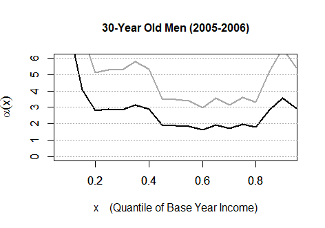
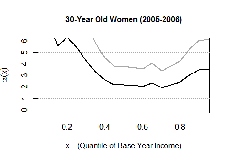
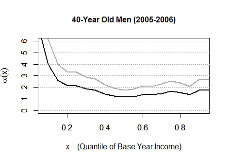
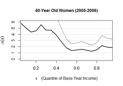
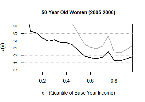
Figure 8: Estimates (black lines) and the one-sided 95% confidence intervals (gray lines) of the Pareto exponents $\alpha(x_{0})$ of the conditional tail risk for men (left) and women (right) based on the NESPD in the period 2005–2006. The left (respectively, right) column shows the results for men (respectively, women). The top, middle, and bottom panels show results for 30-, 40- and 50-year-old individuals. Number of individuals: 48,542 men (47,851 women).

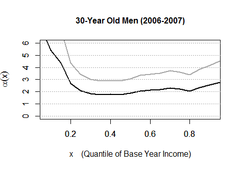
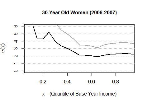
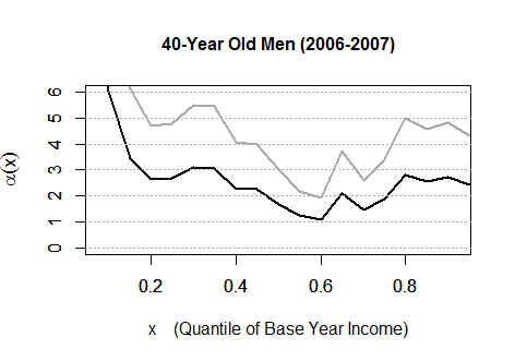
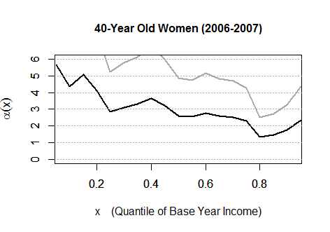
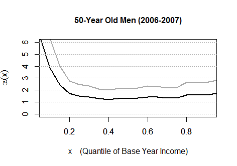
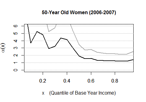
Figure 9: Estimates (black lines) and the one-sided 95% confidence intervals (gray lines) of the Pareto exponents $\alpha(x_{0})$ of the conditional tail risk for men (left) and women (right) based on the NESPD in the period 2006–2007. The left (respectively, right) column shows the results for men (respectively, women). The top, middle, and bottom panels show results for 30-, 40- and 50-year-old individuals. Number of individuals: 39,903 men (39,546 women).

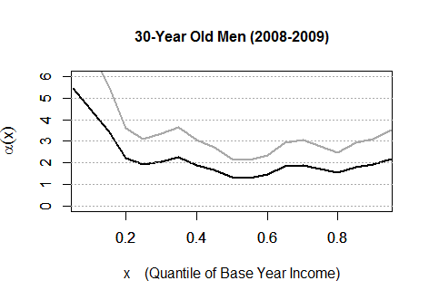
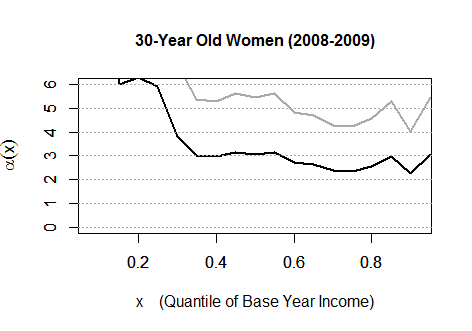
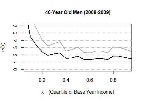
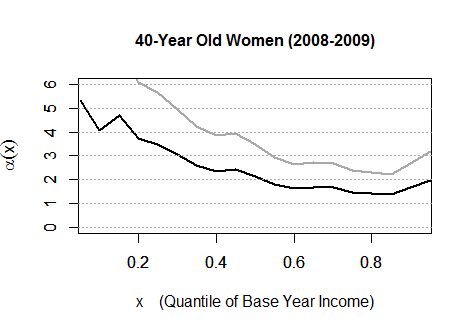
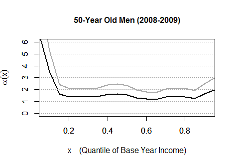
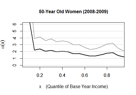
Figure 10: Estimates (black lines) and the one-sided 95% confidence intervals (gray lines) of the Pareto exponents $\alpha(x_{0})$ of the conditional tail risk for men (left) and women (right) based on the NESPD in the period 2008–2009. The left (respectively, right) column shows the results for men (respectively, women). The top, middle, and bottom panels show results for 30-, 40- and 50-year-old individuals. Number of individuals: 39,715 men (40,449 women).

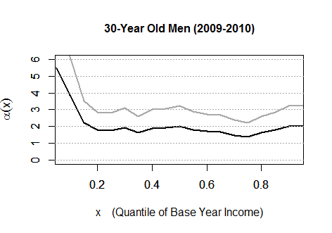
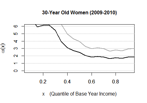
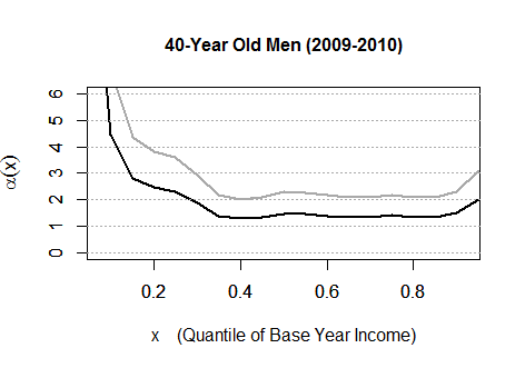
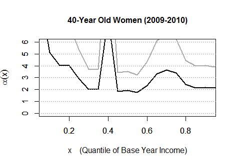
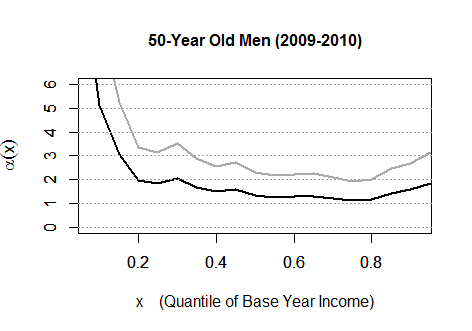
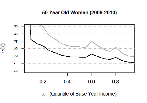
Figure 11: Estimates (black lines) and the one-sided 95% confidence intervals (gray lines) of the Pareto exponents $\alpha(x_{0})$ of the conditional tail risk for men (left) and women (right) based on the NESPD in the period 2009–2010. The left (respectively, right) column shows the results for men (respectively, women). The top, middle, and bottom panels show results for 30-, 40- and 50-year-old individuals. Number of individuals: 48,368 men (50,372 women).

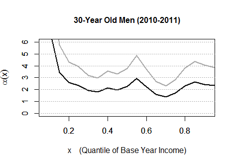
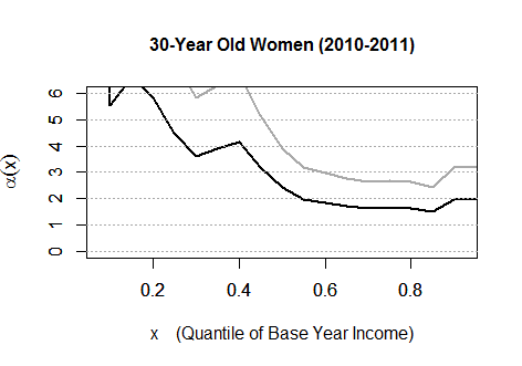
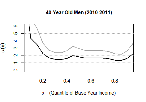
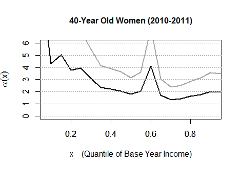
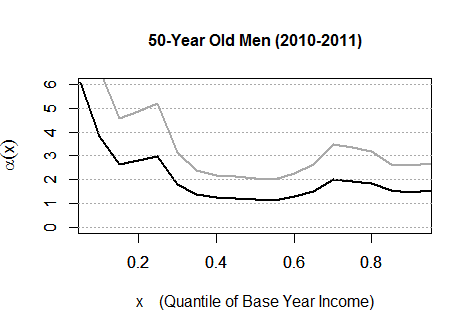
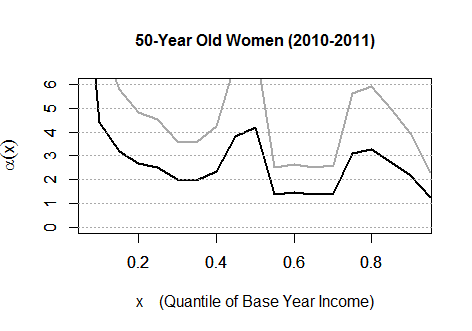
Figure 12: Estimates (black lines) and the one-sided 95% confidence intervals (gray lines) of the Pareto exponents $\alpha(x_{0})$ of the conditional tail risk for men (left) and women (right) based on the NESPD in the period 2010–2011. The left (respectively, right) column shows the results for men (respectively, women). The top, middle, and bottom panels show results for 30-, 40- and 50-year-old individuals. Number of individuals: 49,367 men (51,672 women).

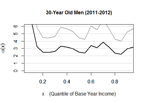
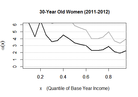
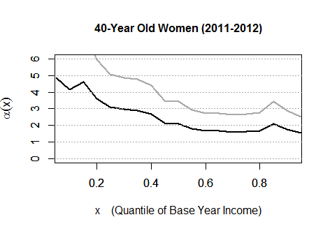
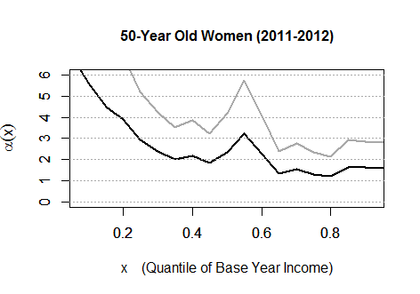
Figure 13: Estimates (black lines) and the one-sided 95% confidence intervals (gray lines) of the Pareto exponents $\alpha(x_{0})$ of the conditional tail risk for men (left) and women (right) based on the NESPD in the period 2011–2012. The left (respectively, right) column shows the results for men (respectively, women). The top, middle, and bottom panels show results for 30-, 40- and 50-year-old individuals. Number of individuals: 49,720 men (52,874 women).

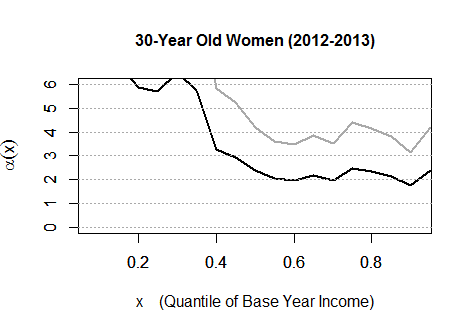
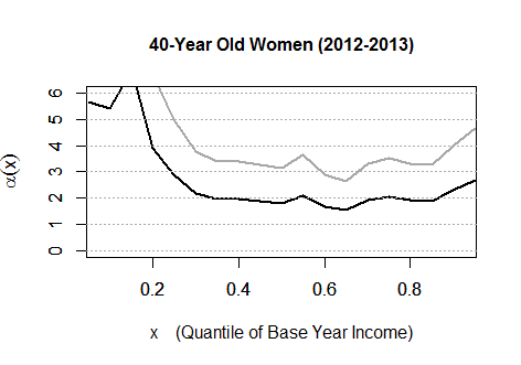
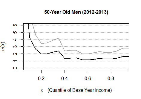
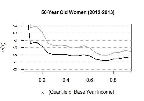
Figure 14: Estimates (black lines) and the one-sided 95% confidence intervals (gray lines) of the Pareto exponents $\alpha(x_{0})$ of the conditional tail risk for men (left) and women (right) based on the NESPD in the period 2012–2013. The left (respectively, right) column shows the results for men (respectively, women). The top, middle, and bottom panels show results for 30-, 40- and 50-year-old individuals. Number of individuals: 48,728 men (51,799 women).

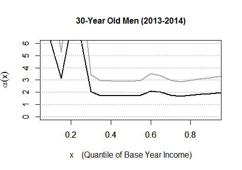
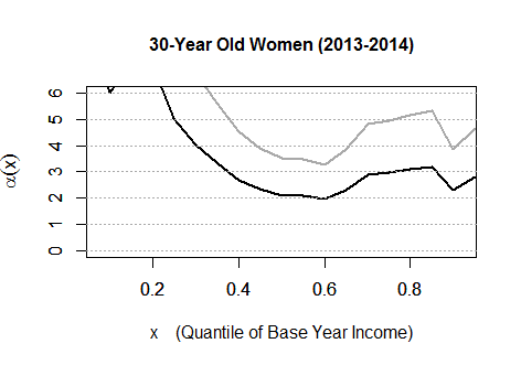
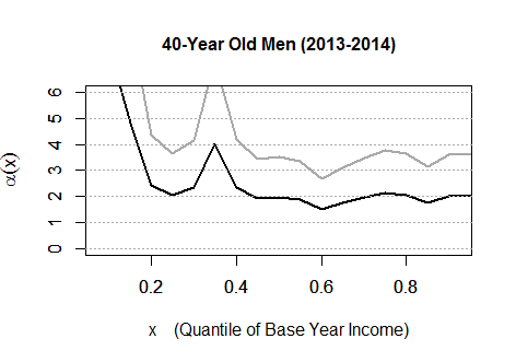
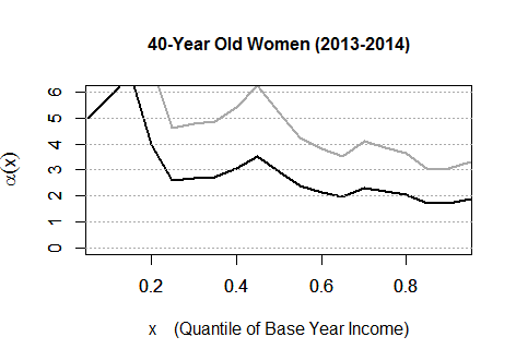
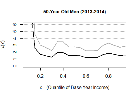
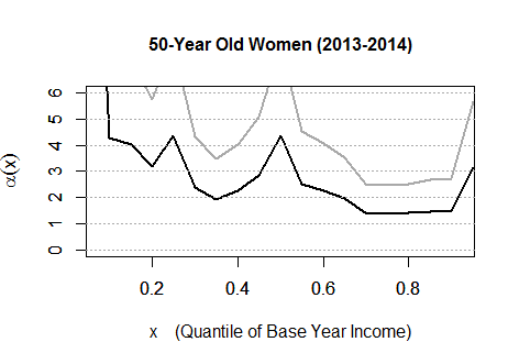
Figure 15: Estimates (black lines) and the one-sided 95% confidence intervals (gray lines) of the Pareto exponents $\alpha(x_{0})$ of the conditional tail risk for men (left) and women (right) based on the NESPD in the period 2013–2014. The left (respectively, right) column shows the results for men (respectively, women). The top, middle, and bottom panels show results for 30-, 40- and 50-year-old individuals. Number of individuals: 49,455 men (52,586 women).

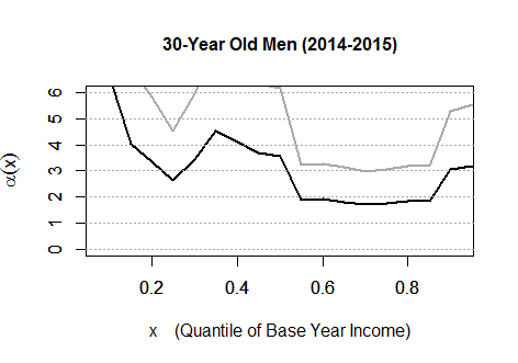
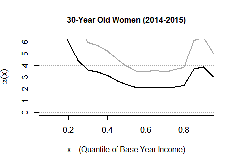
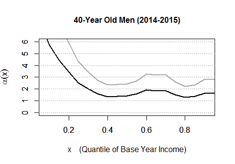
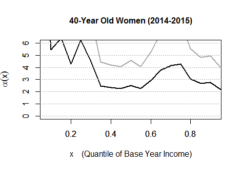
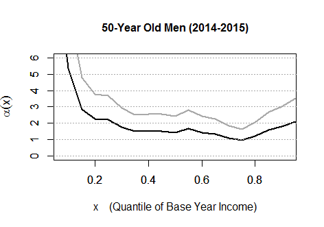
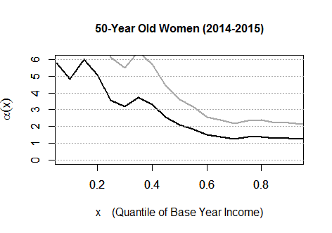
Figure 16: Estimates (black lines) and the one-sided 95% confidence intervals (gray lines) of the Pareto exponents $\alpha(x_{0})$ of the conditional tail risk for men (left) and women (right) based on the NESPD in the period 2014–2015. The left (respectively, right) column shows the results for men (respectively, women). The top, middle, and bottom panels show results for 30-, 40- and 50-year-old individuals. Number of individuals: 48,520 men (52,109 women).

Appendix C Panel Study of Income Dynamics

C.1 Data

We also apply our methodology to another data set, the US Panel Study of Income Dynamics (PSID), which is one of the most commonly used data sets for empirical research on income dynamics. The portion of data for the pair, 2007 and 2009, of years across the period of the great recession is extracted for our use. We select the subsample of both men and women whose total taxable incomes were recorded and non-zero in both 2007 and 2009 and were aged between 25 and 64 in 2007. This sample selection leaves 271 individuals. For the purpose of comparisons, we also use the portion of data for the pair, 2017 and 2019, of the most recent survey years at the time of our writing of this paper. Note that this period is associated with positive economic growth in the United States. The sample selection procedure described above leaves 389 individuals for this period.

We define a measure $Y$ as the absolute difference of the log income in 2007 and the log income in 2009 (i.e., two-year income growth rate). Similarly, we also construct this variable for the period between 2017 and 2019. Figures 17 and 18 display kernel density estimates of the income measure $Y$ for the period 2007–2009 and the period 2017–2019, respectively. In each figure, the left and right panels show the densities for men and women, respectively. Also shown in gray dashed lines are the normal density plots fit to data. Observe that each kernel density exhibits a large spike in the middle of the distribution sticking upward out of the reference normal density. Moreover, each kernel density has heavier tails compared to the reference normal density. These features of the estimated densities evidence that the actual distributions of $Y$ indeed have heavier tails than normal distributions, as documented in the previous literature. That said, as emphasized in the introductory section, nonparametric density plots cannot informatively demonstrate evidence of heavy tails.

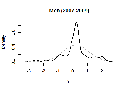
Figure 17: Kernel density estimates (black line) of the risk measure $Y$ in 2007 in the PSID. The right (respectively, left) panel show the density of men (respectively, women). Also shown in gray dashed lines are the normal density fit to data.

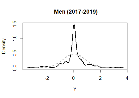
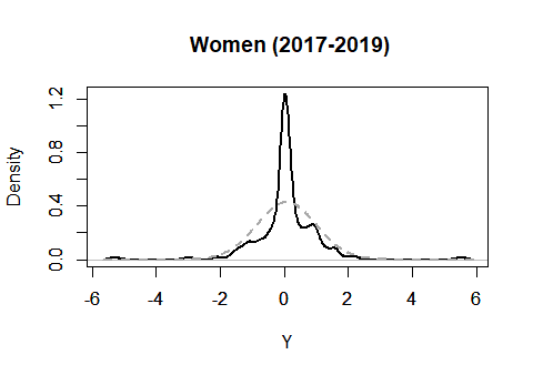
Figure 18: Kernel density estimates (black line) of the risk measure $Y$ in 2017 in the PSID. The right (respectively, left) panel show the density of men (respectively, women). Also shown in gray dashed lines are the normal density fit to data.

We analyze the heaviness of the tails of the conditional distributions of $Y$ given the income level and age in the base year (i.e., the base year is 2007 for the period 2007–2009 and it is 2017 for the period 2017–2019).

C.2 Results

Applying the method introduced in Section 3 (and also Appendix A) to the US Panel Study of Income Dynamics (PSID) described in Appendix C.1, we analyze conditional tail risk of income of adult individuals in the United States. We define $Y$ by the absolute difference of the log income in 2007 and the log income in 2009 for our baseline analysis. For the conditioning variables $X$, we include the quantile of income level and the age of the individual in the base year (2007), following Guvenen et al. (2019). With this setting, we study the conditional Pareto exponent $\alpha(x_{0})$ for each point $x_{0}$ of income levels from $\{0.05,0.10,\cdots,0.90,0.95\}$ (in quantile) and ages from $\{30,40,50\}$ for each of men and women.

Figure 19 illustrates the estimates of the conditional Pareto exponents $\alpha(x_{0})$ (in black lines) along with the upper bounds of their one-sided 95% confidence intervals (in gray lines) for 30-, 40- and 50-year-old individuals, respectively. The top (respectively, bottom) panel shows results for men (respectively, women) in each figure. We observe different patterns of heterogeneous income risk across age, income, and gender groups and describe them in the order of age and gender.

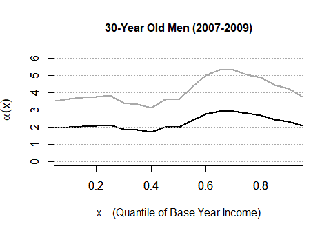
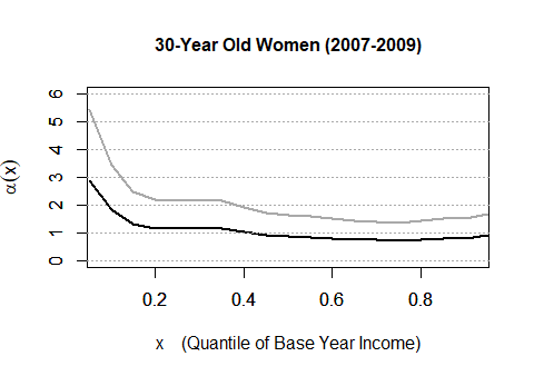
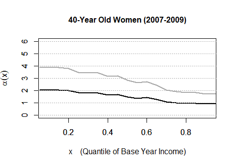
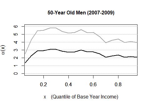
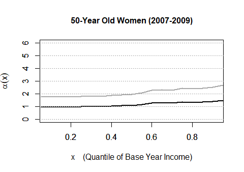
Figure 19: Estimates (black lines) and the one-sided 95% confidence intervals (gray lines) of the Pareto exponents $\alpha(x_{0})$ of the conditional tail risk for men (left) and women (right) based on the PSID in the period 2007–2009. The left (respectively, right) column shows the results for men (respectively, women). The top, middle, and bottom panels show results for 30-, 40- and 50-year-old individuals.

For 30-year-old men (the top left panel in Figure 19), the conditional Pareto exponents (in point estimates) range from 1.7 to 2.9, and the upper bounds of the one-sided 95% confidence intervals range from 3.1 to 5.3. Given that income received in 2007 was at or below the median, the conditional Pareto exponent is significantly less than four, implying that the conditional kurtosis of income growth does not exist for these lower-income groups of young men. The same conclusion also applies to the very top quantiles (top 5 percent). Overall, the kurtosis barely exists for most of the base-year income levels even if we fail to reject the hypothesis of finite kurtosis. For 30-year-old women (the top right panel in Figure 19), the conditional Pareto exponents (in point estimates) range from 0.7 to 2.9, and the upper bounds of the one-sided 95% confidence intervals range from 1.4 to 5.4. For this subpopulation, the conditional Pareto exponent is significantly less than four except for the very bottom quantiles (bottom 5 percent), implying that the conditional kurtosis does not exist. Furthermore, given that income received in 2007 was at or above the 15th (respectively, 40th) percentile, the Pareto exponent is significantly less than three (respectively, two), implying that even the conditional skewness (respectively, standard deviation) does not exist. Comparing the results between men and women at age 30, we observe that women were more vulnerable to income risk than men, except at the very bottom quantiles of the base year income level.

For 40-year-old men (the middle left panel in Figure 19), the conditional Pareto exponents (in point estimates) range from 1.2 to 1.6, and the upper bounds of the one-sided 95% confidence intervals range from 2.1 to 2.9. Remarkably, the income risk of 40-year-old men are higher than those of 30-year-old men. For this age group of men, we reject the hypothesis of finite kurtosis at any level of base-year income. For 40-year-old women (the middle right panel in Figure 19), the conditional Pareto exponents (in point estimates) range from 0.9 to 2.0, and the upper bounds of the one-sided 95% confidence intervals range from 1.7 to 3.9. For this age group of women, we reject the hypothesis of finite kurtosis at any income level. Furthermore, given that income received in 2007 was at or above the 50th (respectively, 75th) percentile, the Pareto exponent is significantly less than three (respectively, two), implying that even the conditional skewness (respectively, standard deviation) does not exist. Comparing the results between men and women at age 30, observe that men are almost as vulnerable to income risk as women for this middle age group.

For 50-year-old men (the bottom left panel in Figure 19), the conditional Pareto exponents (in point estimates) range from 1.3 to 3.1, and the upper bounds of the one-sided 95% confidence intervals range from 2.5 to 5.8. For this age group of men, the conditional Pareto exponents are relatively high, and we fail to reject the hypothesis of finite conditional kurtosis except at the very bottom quantiles (bottom 5 percent) of base-year income. For 50-year-old women (the bottom right panel in Figure 19), the conditional Pareto exponents (in point estimates) range from 1.0 to 1.5, and the upper bounds of the one-sided 95% confidence intervals range from 1.7 to 2.7. For this age group of women, we reject the hypothesis of finite conditional skewness at any income level. Furthermore, given that income received in 2007 was at or below the median, the Pareto exponent is significantly less than three, implying that even the conditional skewness does not exist.

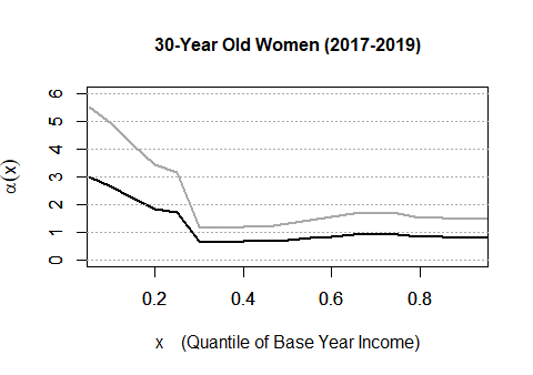
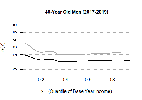
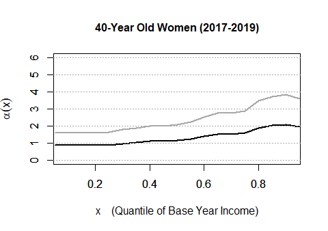
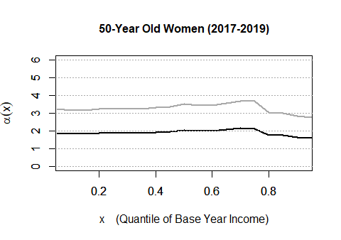
Figure 20: Estimates (black lines) and the one-sided 95% confidence intervals (gray lines) of the Pareto exponents $\alpha(x_{0})$ of the conditional tail risk for men (left) and women (right) based on the PSID in the period 2017–2019. The left (respectively, right) column shows the results for men (respectively, women). The top, middle, and bottom panels show results for 30-, 40- and 50-year-old individuals.

While our main focus has been on the period of great recession between 2007 and 2009, we next look at the period of positive growth, between 2017 and 2019, ten years later than the baseline period. Figure 20 illustrates the results for income growth between 2017 and 2019 for 30-, 40- and 50-year-old individuals, respectively. These results share similar qualitative patterns to those reported in Figures 19 as follows. First, 30-year-old men at high quantiles of base-year income enjoy less income risk. Second, 30-year-old women suffer from high income risk except at the bottom quantiles of base-year income. Third, 40-year-old men have overall higher income risk than 30-year-old men. Lastly, and most remarkably, the income risk is not necessarily lower in the period 2017–2019 than in the period 2007–2009, even though the former period enjoyed a positive GDP growth (5.2% in two years) and the latter period suffered from negative GDP growth ($-$2.7% in two years). With all these similarities, there are differences as well – especially in the graphs that do not resemble across the period between 2017 and 2019 and the period between 2007 and 2009 for 40-year-old women or 50-year-old men. Overall, there are more similarities than differences despite the contrast between a recession and a positive growth in the US economy.

We repeat the econometric analysis for the remaining periods, 2009–2011, 2011–2013, 2013–2015 and 2015–2017 to demonstrate the robustness of the observed patterns reported above. Figures 21, 22, 23 and 24 illustrate estimates of the conditional Pareto exponents $\alpha(x_{0})$ (in black lines) along with the upper bounds of their one-sided 95% confidence intervals (in gray lines) for the periods 2009–2011, 2011–2013, 2013–2015 and 2015–2017. In each figure, the left (respectively, right) column shows the results for men (respectiely, women). The top, middle, and bottom panels show results for 30-, 40- and 50-year-old individuals.

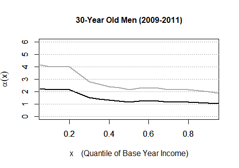
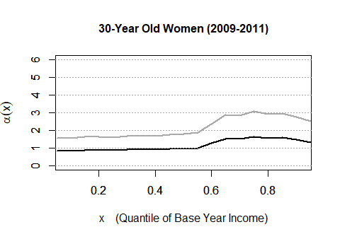
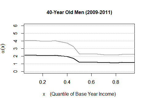
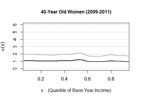
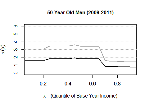
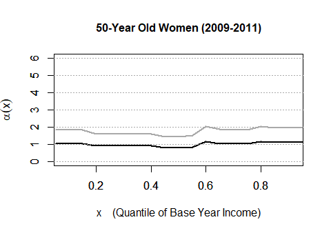
Figure 21: Estimates (black lines) and the one-sided 95% confidence intervals (gray lines) of the Pareto exponents $\alpha(x_{0})$ of the conditional tail risk for men (left) and women (right) based on the PSID in the period 2009–2011. The left (respectively, right) column shows the results for men (respectively, women). The top, middle, and bottom panels show results for 30-, 40- and 50-year-old individuals.

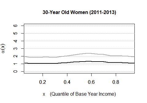
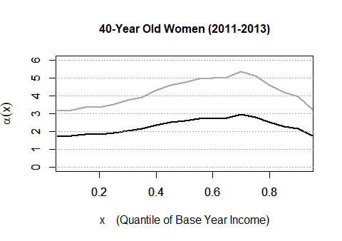
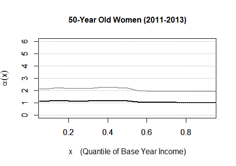
Figure 22: Estimates (black lines) and the one-sided 95% confidence intervals (gray lines) of the Pareto exponents $\alpha(x_{0})$ of the conditional tail risk for men (left) and women (right) based on the PSID in the period 2011–2013. The left (respectively, right) column shows the results for men (respectively, women). The top, middle, and bottom panels show results for 30-, 40- and 50-year-old individuals.

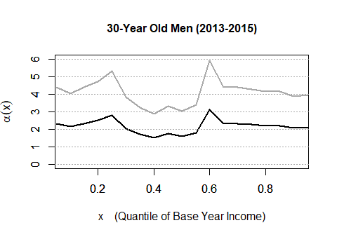
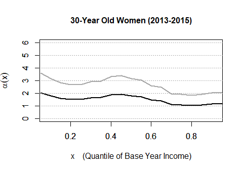
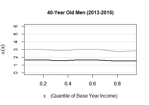
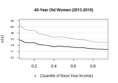
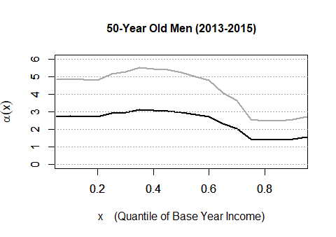
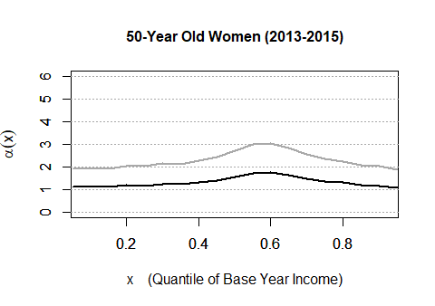
Figure 23: Estimates (black lines) and the one-sided 95% confidence intervals (gray lines) of the Pareto exponents $\alpha(x_{0})$ of the conditional tail risk for men (left) and women (right) based on the PSID in the period 2013–2015. The left (respectively, right) column shows the results for men (respectively, women). The top, middle, and bottom panels show results for 30-, 40- and 50-year-old individuals.

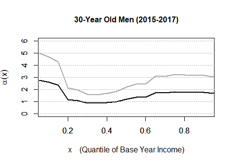
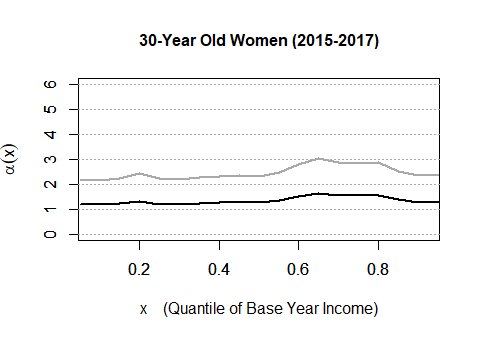
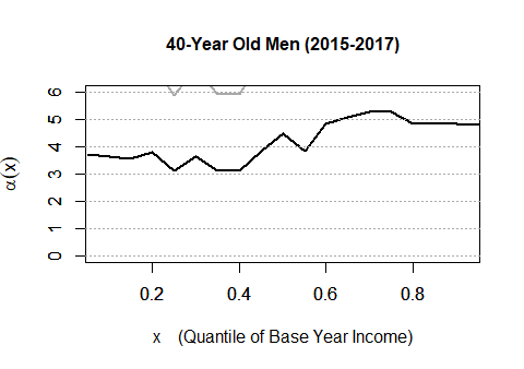
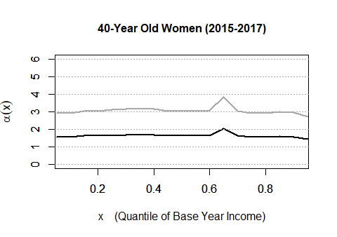
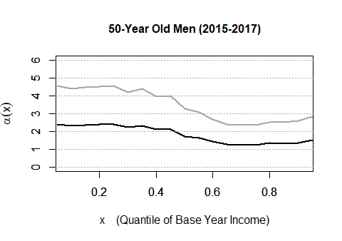
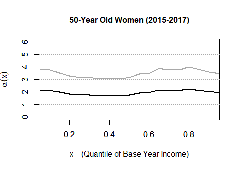
Figure 24: Estimates (black lines) and the one-sided 95% confidence intervals (gray lines) of the Pareto exponents $\alpha(x_{0})$ of the conditional tail risk for men (left) and women (right) based on the PSID in the period 2015–2017. The left (respectively, right) column shows the results for men (respectively, women). The top, middle, and bottom panels show results for 30-, 40- and 50-year-old individuals.

For the periods 2007–2009 and 2017–2019 we found that: 1) the kurtosis, skewness, and even standard deviation may not exist for the conditional distribution of income growth given certain attributes (age, gender, and income); 2) younger women are more vulnerable to income risk than younger men; 3) middle-aged men are almost as vulnerable as middle-aged women; and 4) these patterns appear both in the period 2007–2009 of great recession and the period 2017–2019 of a positive growth, while there are differences as well. The first and second points robustly hold in the remaining periods, 2009–2011, 2011–2013, 2013–2015 and 2015–2017. The third point also continues to hold for the periods, 2009–2011 (to a less extent), 2011–2013 and 2013–2015. Thus, the fourth point largely extends to the remaining periods, 2009–2011, 2011–2013, 2013–2015 and 2015–2017.

Data Citation: Office for National Statistics. (2017). New Earnings Survey Panel Dataset, 1975-2016: Secure Access. [data collection]. 7th Edition. UK Data Service. SN: 6706, http://doi.org/10.5255/UKDA-SN-6706-7

References

- Adam et al. (2019) Stuart Adam, David Phillips, and Barra Roantree. 35 years of reforms: A panel analysis of the incidence of, and employee and employer responses to, social security contributions in the uk. Journal of Public Economics, 171:29–50, 2019.
- Arellano et al. (2017) Manuel Arellano, Richard Blundell, and Stéphane Bonhomme. Earnings and consumption dynamics: a nonlinear panel data framework. Econometrica, 85(3):693–734, 2017.
- Arellano et al. (2021) Manuel Arellano, Stéphane Bonhomme, Micole De Vera, Laura Hospido, and Sizi Wei. Income risk inequality: evidence from spanish administrative records. Working Paper, 2021.
- Beare and Toda (2017) Brendan K Beare and Alexis Akira Toda. Determination of pareto exponents in economic models driven by markov multiplicative processes. arXiv preprint arXiv:1712.01431, 2017.
- Bell et al. (2021) Brian D Bell, Nicholas Bloom, and Jack Blundell. This time is not so different: Income dynamics during the covid-19 recession. 2021.
- Bhattacharya (1984) P. K. Bhattacharya. Induced Order Statistics: Theory and Applications, chapter 18, pages 383–403. Elsevier Sicence Publishers, 1984.
- Bonhomme and Robin (2009) Stéphane Bonhomme and Jean-Marc Robin. Assessing the equalizing force of mobility using short panels: France, 1990–2000. The Review of Economic Studies, 76(1):63–92, 2009.
- Bonhomme and Robin (2010) Stéphane Bonhomme and Jean-Marc Robin. Generalized non-parametric deconvolution with an application to earnings dynamics. The Review of Economic Studies, 77(2):491–533, 2010.
- Botosaru and Sasaki (2018) Irene Botosaru and Yuya Sasaki. Nonparametric heteroskedasticity in persistent panel processes: An application to earnings dynamics. Journal of Econometrics, 203(2):283–296, 2018.
- Chernozhukov et al. (2018) Victor Chernozhukov, Denis Chetverikov, Mert Demirer, Esther Duflo, Christian Hansen, Whitney Newey, and James Robins. Double/debiased machine learning for treatment and structural parameters. The Econometrics Journal, 21(1):C1–C68, 01 2018. doi: 10.1111/ectj.12097.
- de Haan and Ferreira (2007) Laurens de Haan and Ana Ferreira. Extreme Value Theory: An Introduction. Springer Series in Operations Research and Financial Engineering. Springer, NY, 2007.
- De Nardi et al. (2021) Mariacristina De Nardi, Giulio Fella, and Gonzalo Paz-Pardo. Wage risk and government and spousal insurance. Technical report, National Bureau of Economic Research, 2021.
- Degiannakis et al. (2022) Stavros Degiannakis, George Filis, Grigorios Siourounis, and Lorenzo Trapani. Superkurtosis. Forthcoming in Journal of Money, Credit and Banking, 2022.
- Elsby et al. (2016) Michael WL Elsby, Donggyun Shin, and Gary Solon. Wage adjustment in the great recession and other downturns: Evidence from the united states and great britain. Journal of Labor Economics, 34(S1):S249–S291, 2016.
- Gabaix (2009) Xavier Gabaix. Power laws in economics and finance. Annual Review of Economics, 1:255–293, 2009.
- Gabaix (2016) Xavier Gabaix. Power laws in economics: An introduction. Journal of Economic Perspectives, 30(1):185–206, 2016.
- Gabaix and Ibragimov (2011) Xavier Gabaix and Rustam Ibragimov. Rank: A simple way to improve the OLS estimation of tail exponents. Journal of Business and Economic Statistics, 29(1):24–39, January 2011. doi: 10.1198/jbes.2009.06157.
- Gardes and Girard (2008) Laurent Gardes and Stéphane Girard. A moving window approach for nonparametric estimation of the conditional tail index. Journal of Multivariate Analysis, 99:2368–2388, 2008.
- Gardes et al. (2012) Laurent Gardes, Armelle Guillou, and Antoine Schorgen. Estimating the conditional tail index by integrating a kernel conditional quantile estimator. Journal of Statistical Planning and Inference, 142:1586–1598, 2012.
- Geweke and Keane (2000) John Geweke and Michael Keane. An empirical analysis of earnings dynamics among men in the psid: 1968–1989. Journal of econometrics, 96(2):293–356, 2000.
- Golosov et al. (2016) Mikhail Golosov, Maxim Troshkin, and Aleh Tsyvinski. Redistribution and social insurance. American Economic Review, 106(2):359–86, 2016.
- Goos and Manning (2007) Maarten Goos and Alan Manning. Lousy and lovely jobs: The rising polarization of work in britain. The review of economics and statistics, 89(1):118–133, 2007.
- Guillou and Hall (2001) Armelle Guillou and Peter Hall. A diagnostic for selecting the threshold in extreme value analysis. Journal of Royal Statistic Society, Series B, 63:293–305, 2001.
- Guvenen et al. (2019) Fatih Guvenen, Fatih Karahan, Serdar Ozkan, and Jae Song. What do data on millions of us workers reveal about life-cycle earnings dynamics? Federal Reserve Bank of New York Staff Report, 2019.
- Hill (1975) Bruce M. Hill. A simple general approach to inference about the tail of a distribution. Annals of Statistics, 3(5):1163–1174, September 1975. doi: 10.1214/aos/1176343247.
- Horowitz and Markatou (1996) Joel L Horowitz and Marianthi Markatou. Semiparametric estimation of regression models for panel data. The Review of Economic Studies, 63(1):145–168, 1996.
- Hu et al. (2019) Yingyao Hu, Robert Moffitt, and Yuya Sasaki. Semiparametric estimation of the canonical permanent-transitory model of earnings dynamics. Quantitative Economics, 10(4):1495–1536, 2019.
- Moffitt and Zhang (2018) Robert Moffitt and Sisi Zhang. Income volatility and the psid: Past research and new results. In AEA Papers and Proceedings, volume 108, pages 277–80, 2018.
- Nickell and Quintini (2003) Stephen Nickell and Glenda Quintini. Nominal wage rigidity and the rate of inflation. The Economic Journal, 113(490):762–781, 2003.
- Sasaki and Wang (2022) Yuya Sasaki and Yulong Wang. Fixed-k inference for conditional extremal quantiles. Journal of Business & Economic Statistics, 40(2):829–837, 2022.
- Smith (1987) Richard L. Smith. Estimating tails of probability distributions. Annals of Statistics, 15(3):1174–1207, September 1987. doi: 10.1214/aos/1176350499.
- Trapani (2016) Lorenzo Trapani. Testing for (in) finite moments. Journal of Econometrics, 191(1):57–68, 2016.
- Wang and Tsai (2009) Hansheng Wang and Chi-Ling Tsai. Tail index regression. Journal of the American Statistical Association, 104:1233–1240, 2009.
- Wang and Li (2013) Huixia Judy Wang and Deyuan Li. Estimation of extreme conditional quantiles through power transformation. Journal of the American Statistical Association, 108(503):1062–1074, 2013. doi: 10.1080/01621459.2013.820134.