Better Uncertainty Calibration via Proper Scores for Classification and Beyond

Abstract

With model trustworthiness being crucial for sensitive real-world applications, practitioners are putting more and more focus on improving the uncertainty calibration of deep neural networks. Calibration errors are designed to quantify the reliability of probabilistic predictions but their estimators are usually biased and inconsistent. In this work, we introduce the framework of proper calibration errors, which relates every calibration error to a proper score and provides a respective upper bound with optimal estimation properties. This relationship can be used to reliably quantify the model calibration improvement. We theoretically and empirically demonstrate the shortcomings of commonly used estimators compared to our approach. Due to the wide applicability of proper scores, this gives a natural extension of recalibration beyond classification.

1 Introduction

Deep learning became a dominant cornerstone of machine learning research in the last decade and deep neural networks can surpass human-level predictive performance on a wide range of tasks [19, 47, 17]. However, Guo et al. [14] have shown that for modern neural networks, better classification accuracy can come at the cost of systematic overconfidence in their predictions. Practitioners in sensitive forecasting domains, such as cancer diagnostics [17], genotype-based disease prediction [25] or climate prediction [59], require for models to not only have high predictive power but also to reliably communicate uncertainty. This raises the need to quantify and improve the quality of predictive uncertainty, ideally via a dedicated metric. An uncertainty-aware model should give probabilistic predictions which represent the true likelihood of events depending on the very prediction. To quantify the extend to which this condition is violated, calibration errors have been introduced. In general, their estimators are usually biased [46] and inconsistent [53]. This, in turn, is highly problematic since we cannot quantify how reliable a model is if we do not know how reliable the metric is. Especially the medical field is a domain that requires high model trustworthiness, but with low expert availability and/or disease frequency we often encounter a small data regime. Resampling strategies can be viable options for optimization on small datasets but also reduce the evaluation set size even more. We will discover that little data exacerbates the estimation bias and propose reliable alternatives for improving uncertainty calibration.

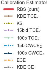
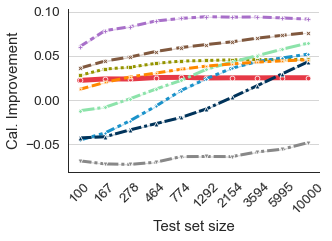
(a) TS of DenseNet 40 on
CIFAR10

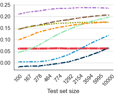
(b) ETS of Wide ResNet 32
on CIFAR100

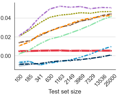
(c) DIAG of DenseNet 161 on ImageNet

Figure 1: Estimated calibration improvement for various settings. The calibration error is estimated before and after a recalibration method (TS / ETS / DIAG) is applied and the difference (i.e. calibration improvement) is shown for increasing test set size. All common calibration estimators are sensitive with respect to the test set size and can substantially over- or underestimate the effect of performing recalibration.Only RBS robustly estimates the improvement in calibration error for all test set sizes.

Since deep neural networks often yield uncalibrated confidence scores [36], a variety of different post-hoc recalibration approaches have been proposed [7, 31]. These methods use the validation set to transform predictions returned by a trained neural network such that they become better calibrated. A key desired property of recalibration methods is to not reduce the accuracy after the transformation. Therefore, most modern approaches are restricted to accuracy preserving transformations of the model outputs [42, 14, 63, 45]. When recalibrating a model, it is crucial to have a reliable estimate of how much the chosen method improves the underlying model. However, when using current estimators for calibration errors, their biased nature results in estimates that are highly sensitive to the number of samples in the test set that are used to compute the calibration error before and after recalibration (Fig. 2; c.f. Section 5). The source code is openly available at https://github.com/MLO-lab/better_uncertainty_calibration.

Our contributions for better uncertainty calibration are summarized in the following. We…

• … give an overview of current calibration error literature, place the errors into a taxonomy, and show which are insufficient for calibration quantification. This also includes several theoretical results, which highlight the shortcomings of current approaches.

• … introduce the framework of proper calibration errors, which gives important guarantees and relates every element to a proper score. We can reliably estimate the improvement of an injective recalibration method w.r.t. a proper calibration error via its related proper score - even in non-classification settings.

• … show that common calibration estimators are highly sensitive w.r.t. the test set size. We demonstrate that for commonly used estimators, the estimated improvement of recalibration methods is heavily biased and becomes monotonically worse with fewer test data.

2 Related Work

In this section, we give an extensive overview of published work regarding quantifying model calibration and model recalibration. Important definitions will be directly given, while others are placed in Appendix C. These will be the basis for our theoretical findings. Further, we will motivate the definition of proper calibration errors, which are directly related to proper scores. Consequently, we will also present important aspects of the framework around proper scores in later parts of this section.

2.1 Calibration errors

For clarity, we introduce shortly the notation used throughout this work. Assume we have random variables $X$ and $Y$ corresponding to feature and target variable, and feature and target space $\mathscr{X}$ and $\mathscr{Y}$. We have $\mathbb{P}_{Y},\mathbb{P}_{Y\mid X}\in\mathscr{P}$, where $\mathbb{P}_{Y}$ refers to the distribution of $Y$, $\mathbb{P}_{Y\mid X}$ to the conditional distribution given $X$, and $\mathscr{P}$ a set of distributions on $\mathscr{Y}$. Even though some approaches explore calibration for regression tasks [48, 58, 6], it is most dominantly considered for classification. To distinguish between the general case and $n$-class classification, we refer to $\mathscr{P}_{n}$ as the $n$-dimensional simplex of corresponding categorical distributions.

A popular task is the calibration of the predicted top-label $C=\arg\max_{k}f_{k}\left(X\right)$ of a model $f\colon\mathscr{X}\to\mathscr{P}_{n}$ [14, 30, 34, 41, 53, 51, 45]. Here, the top-label confidence should represent the accuracy of this very prediction. Formally, we try to reach the condition $f_{C}\left(X\right)=\mathbb{P}\left(Y=C\mid f_{C}\left(X\right)\right)$. However, the condition is weaker as one might expect, and referring to a model fulfilling this condition as (perfectly) calibrated can give a false sense of security [53, 57]. This holds especially in forecasting domains, where low probability estimates can still be highly relevant. For example, assigning probability mass to an aggressive type of cancer can still trigger action even if it is not predicted as the most likely outcome. Further, we might also be interested in predictive uncertainty for non-classification tasks. Consequently, we use the stricter and more general condition that the complete prediction $f\left(X\right)$ should be equal to the complete conditional distribution $\mathbb{P}_{Y\mid f\left(X\right)}$ of the target given this very prediction as introduced by Widmann et al. [58]. More formally, we state:

Definition 2.1.

A model $f\colon\mathscr{X}\to\mathscr{P}$ is calibrated if and only if $f\left(X\right)=\mathbb{P}_{Y\mid f\left(X\right)}$.

Note that $\mathscr{P}$ can be a set of arbitrary distributions, which incorporates $\mathscr{P}_{n}$ (classification) as a special case.

One of the first metrics for assessing model calibration that is still widely used in recent literature is the Brier score (BS) [38, 42, 16, 45]. For a model $f\colon\mathscr{X}\to\mathscr{P}_{n}$ the Brier score [3] is defined as

$$\text{BS}\left(f\right)=\mathbb{E}\left[\left\|f\left(X\right)-Y^{\prime}\right\|^{2}_{2}\right],$$ (1)

where $Y^{\prime}$ is one-hot-encoded $Y$. The estimator of the BS is equivalent to the mean squared error, illustrating that it does not purely capture model calibration. Rather, the BS can be interpreted as a comprehensive measure of model performance, simultaneously capturing model fit and calibration. This becomes more obvious via the canonical decomposition of the BS into a calibration and sharpness term [38]. Based on this decomposition, we can derive the following error. For $1\leq p\in\mathbb{R}$, the $L^{p}$ calibration error (CE_p) of model $f\colon\mathscr{X}\to\mathscr{P}_{n}$ is defined as

$$\text{CE}_{p}\left(f\right)=\left(\mathbb{E}\left[\left\|f\left(X\right)-\mathbb{P}_{Y\mid f\left(X\right)}\right\|^{p}_{p}\right]\right)^{\frac{1}{p}}.$$ (2)

The BS decomposition only supports the squared case, but a general $L^{p}$ formulation became more common in recent years [53, 57, 63, 43]. Popordanoska et al. [43] proposed to estimate CE_p via multivariate kernel density estimation. In general, calibration estimation is difficult due to the term $\mathbb{P}_{Y\mid f\left(X\right)}$ since we never have samples of every possible prediction for continuous models. This is in contrast to the original work of Murphy [38], where only models with a finite prediction space are considered. To assess the calibration of a continuous binary model Platt [42] used histogram estimation, transforming the infinite prediction space to a finite one. This is also referred to as equal width binning. Similarly, Nguyen & O’Connor [40] introduced an equal mass binning scheme for continuous binary models. Both, equal width and equal mass binning schemes, suffer from the requirement of setting a hyperparameter. This can significantly influence the estimated value [31] and there is no optimal default since every setting has a different bias-variance tradeoff [41]. The first calibration estimator for a continuous one-vs-all multi-class model was given by Naeini et al. [39] and is still the most commonly used measure to quantify calibration. It is referred to as the expected calibration error (ECE) of model $f\colon\mathscr{X}\to\mathscr{P}_{n}$ and defined as

$$\begin{split}&\text{ECE}\left(f\right)=\sum_{i=1}^{m}p_{i}\left\lvert\text{conf}_{i}-\text{acc}_{i}\right\rvert\end{split}$$ (3)

with the bin frequency $p_{i}=\mathbb{P}\left(f_{C}\left(X\right)\in B_{i}\right)$, the bin-wise mean confidence $\text{conf}_{i}=\mathbb{E}\left[f_{C}\left(X\right)\mid f_{C}\left(X\right)\in B_{i}\right]$, and the bin-wise accuracy $\text{acc}_{i}=\mathbb{P}\left(Y=C\mid f_{C}\left(X\right)\in B_{i}\right)$, for $m\in\mathbb{N}$ bins $B_{i}\coloneqq\left(\frac{i-1}{m},\frac{i}{m}\right]$. We can estimate $p_{i}$, $\text{conf}_{i}$, and $\text{acc}_{i}$ via the respective means. These are then used in equation (3) to estimate the ECE. This estimator is biased [31, 53].

Kull et al. [29] and Nixon et al. [41] independently introduced another calibration estimator, which also captures the extend to which the condition $\mathbb{P}\left(Y=k\mid f_{k}\left(X\right)\right)=f_{k}\left(X\right)$ is violated for each class $k\in\mathscr{Y}$. They respectively use equal width and equal mass binning. Similar to these estimators, Kumar et al. [31] introduced the class-wise calibration error (CWCE_p) and, similar to the ECE, the top-label calibration error (TCE_p). They only formulated the squared case $p=2$ but suggested the extension of their definitions to general $p$-norms, which we provide in Appendix C.

Furthermore, Kumar et al. [31] and Vaicenavicius et al. [53] proved independently that using a fixed binning scheme for estimation leads to a lower bound of the expected error. Zhang et al. [63] circumvent binning schemes by using kernel density estimation to estimate the TCE_p.

Orthogonal ways to quantify model miscalibration have been proposed to not depend on binning or kernel density estimation schemes. Gupta et al. [16] introduced the Kolmogorov-Smirnov calibration error (KS) (c.f. Appendix C), which is based on the Kolmogorov-Smirnov test between empirical cumulative distribution functions. Its estimator does not require setting a hyperparameter but the authors did not provide further theoretical aspects.

Estimators of the TCE_p and CWCE_p are in general not differentiable. Consequently, Kumar et al. [30] proposed the Maximum mean calibration error (MMCE) (c.f. Appendix C), which has a differentiable estimator. It is a kernel-based error, comparing the top-label confidence and the conditional accuracy, similar to the ECE.

Widmann et al. [57] argued that the MMCE is insufficient for quantifying calibration of a model, similar as the ECE. They further proposed the Kernel calibration error (KCE) (c.f. Appendix C). It is based on matrix-valued kernels and unlike the MMCE, which only uses the top-label prediction, includes the whole model prediction. The squared KCE has an unbiased estimator based on a U-statistic with quadratic runtime complexity with respect to the data size. However, even though the KCE is positive, the U-statistic estimator can give negative values. To this end, the authors use the estimated value as a test statistic w.r.t. the null hypothesis that the model is calibrated.

Furthermore, Widmann et al. [57] and Widmann et al. [58] proposed to unify different definitions of calibration errors in a theoretical framework, which also includes variance regression calibration. However, the framework allows calibration errors, which are zero even if the model is not calibrated at all.

2.2 Recalibration

A plethora of recalibration methods have been proposed to improve model calibration after training by transforming the model output probabilities [18, 42, 60, 61, 39, 40, 28, 14, 29, 31, 63, 16, 45]. These methods are optimized on a specific calibration set, which is usually the validation set. Key desiderata of these methods include for the algorithms to be accuracy-preserving and data-efficient [63], reflecting that typical use-cases include settings in sensitive domains where accuracy should remain unchanged and often little data is available to train and evaluate the models. Such accuracy-preserving methods only adjust the probability estimate in such a way that the predicted top-label remains the same. The most commonly used accuracy-preserving recalibration method is temperature scaling (TS) [14], where the model logits are divided by a single parameter $T\in\mathbb{R}_{>0}$ before computing the predictions via softmax. A more expressive extension of TS is ensemble temperature scaling (ETS) [63], where a weighted ensemble of TS output, model output, and label smoothing is computed. Rahimi et al. [45] proposed different classes of order-preserving transformations. A specifically interesting one is the class of diagonal intra order-preserving functions (DIAG). Here, the model logits are transformed elementwise with a scalar, monotonic, and continuous function, which is represented by neural networks of unconstrained monotonic functions [55].

2.3 Proper scores

Gneiting & Raftery [13] give an extensive overview of proper scores. Unfortunately, their presented definitions assume maximization as the model training objective. To stay in line with recent machine learning literature, we flip the sign when it is required in the following definitions, similar as in [4]. We specifically do not constrain ourselves to classification, which is a special case. Assume we give a prediction in $\mathscr{P}$ for an event in $\mathscr{Y}$ and we want to score how good the prediction was. A function $S\;\colon\;\mathscr{P}\times\mathscr{Y}\to\overline{\mathbb{R}}$ with $\overline{\mathbb{R}}\coloneqq\mathbb{R}\cup\left\{-\infty,\infty\right\}$ is called scoring rule or just score. Examples are the Brier score and the log score for classification, or the Dawid-Sebastiani score (DSS), which extends the MSE for variance regression [8, 12]. It is defined as $S\left(P,y\right)=\frac{\left(\mu_{P}-y\right)^{2}}{\sigma_{P}^{2}}+\log\sigma_{P}^{2}$. To compare distributions, we use the expected score $s_{S}\colon\mathscr{P}\times\mathscr{P}\to\mathbb{R}$ defined as $s_{S}\left(P,Q\right)=\mathbb{E}_{Y\sim Q}\left[S\left(P,Y\right)\right]$. A scoring rule $S$ is defined to be proper if and only if $s_{S}\left(P,Q\right)\geq s_{S}\left(Q,Q\right)$ holds for all $P,Q\in\mathscr{P}$, and strictly proper if and only if $P\neq Q\implies s_{S}\left(P,Q\right)>s_{S}\left(Q,Q\right)$. In other words, a score is proper if predicting the target distribution gives the best expected value and strictly proper if no other prediction can achieve this value. Given a proper score $S$ and $P,Q\in\mathscr{P}$, the associated divergence $d_{S}\colon\mathscr{P}\times\mathscr{P}\to\mathbb{R}_{\geq 0}$ is defined as $d_{S}\left(P,Q\right)=s_{S}\left(P,Q\right)-s_{S}\left(Q,Q\right)$ and the associated generalized entropy $g_{S}\colon\mathscr{P}\to\mathbb{R}$ as $g_{S}\left(Q\right)=s_{S}\left(Q,Q\right)$. For strictly proper $S$, $d_{S}$ is only zero if $P=Q$; for (strictly) proper $S$, $g_{S}$ is (strictly) concave. An example of a divergence-entropy combination is the Kullback-Leibler divergence and the Shannon entropy associated to the log score.

Associated entropies and divergences are used in the calibration-sharpness decomposition introduced by Bröcker [4] for proper scores of categorical distributions. In Lemma 4.1 we will prove that this result holds for proper scores of arbitrary distributions, as long as additional conditions are met. Further, associated divergences will be the backbone for our definition of proper calibration errors in Section 4.

3 Theoretical analysis of calibration errors

In this section, we present theoretical results regarding calibration errors used in current literature. First, we place these calibration errors into a taxonomy, which we introduce in Theorem 3.1. Next, we give an example of how much errors lower in the hierarchy can differ from CE₁ in Proposition 3.2. Last, we analyse the ECE estimate with respect to the data size in Proposition 3.3. This proposition is the basis for explaining the empirical (miss-)behaviour of the ECE observed in Section 5. All proofs are presented in Appendix D.

To the best of the authors’ knowledge, other publications provided relations between at most two distinct calibration errors or none at all while introducing a new one. The taxonomy in the following theorem is a novel contribution, improving overview of a whole body of work regarding quantifying calibration.

Theorem 3.1.

Given a model $f\;\colon\;\mathscr{X}\to\mathscr{P}_{n}$ and $1\leq p\in\mathbb{R}$, we have

$$\begin{split}\text{BS}\left(f\right)=0\!\implies\!\!\!\begin{Bmatrix}\text{CE}_{p}\left(f\right)=0\\ \text{KCE}\left(f\right)=0\\ f\text{ calibrated}\end{Bmatrix}\!\!\!\implies\!\text{CWCE}_{p}\left(f\right)=0\!\implies\!\!\!\begin{Bmatrix}\text{TCE}_{p}\left(f\right)=0\\ \text{MMCE}\left(f\right)=0\\ \text{KS}\left(f\right)=0\\ \end{Bmatrix}\!\!\!\implies\!\text{ECE}\left(f\right)=0,\end{split}$$

where statements inside curly brackets $\begin{Bmatrix}\dots\end{Bmatrix}$ are equivalent. Further, we have

$$\begin{split}n^{\frac{1}{p}-\frac{1}{2}}\sqrt{\text{BS}\left(f\right)}\overset{*}{\geq}\text{CE}_{p}\left(f\right)\geq\text{CWCE}_{p}\left(f\right)\geq\text{TCE}_{p}\left(f\right)\geq\text{TCE}_{1}\left(f\right)\geq\begin{cases}\text{KS}\left(f\right)\\ \text{ECE}\left(f\right)\\ c\cdot\text{MMCE}\left(f\right)\end{cases}\geq 0,\end{split}$$

where * only holds for $p\leq 2$. The kernel dependent constant $c\in\mathbb{R}$ is given in Appendix D.2 according to Kumar et al. [30].

From this theorem follows that it is ambiguous to refer to perfect calibration just because there exists a calibration error which is zero for a model. The proof of this theorem also contains $n^{\frac{1}{p}-\frac{1}{q}}\text{CE}_{q}\left(f\right)\geq\text{CE}_{p}\left(f\right)$ for $p\leq q$, which is a contradiction to Theorem 1 in [56]. Next, we demonstrate how large the gap between calibration errors can be.

Proposition 3.2.

Assume the model $f\colon\mathscr{X}\to\mathscr{P}_{n}$ is surjective. There exists a joint distribution of $X$ and $Y$ such that for all $E\in\left\{\text{MMCE},\text{KS},\text{ECE},\text{TCE}_{p},\text{CWCE}_{p}\mid 1\leq p\in\mathbb{R}\right\}\colon$

$$\begin{split}E\left(f\right)=0\quad\text{and}\quad\text{CE}_{2}\left(f\right)\geq\sqrt{0.99-\frac{1}{n}}.\end{split}$$

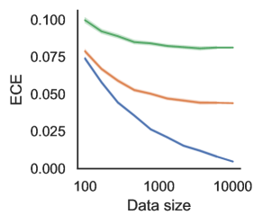
Figure 2: Estimated ECE of simulated models with perfect calibration (blue), mediocre calibration (orange), and bad calibration (green). Better calibration exacerbates ECE bias with respect to the data size, leading to unreliably calibration improvement quantification.

Recall that $\text{CE}_{2}\left(f\right)=0$ if and only if $f$ is calibrated. In other words, most used calibration errors can be zero, but the model is still far from calibrated. An example of a model transformation with perfect ECE but uncalibrated outputs is given in Proposition D.2.

Among all calibration errors, the ECE is still the most commonly used [24, 26, 45, 51, 36, 50, 23, 35, 37, 15, 54, 10], even though its estimator is knowingly biased [31, 46]. Let $\hat{\text{ECE}}_{\left(n\right)}$ denote the ECE estimator for $n$ data instances as originally defined in Guo et al. [14]. The following gives an analysis how this estimate behaves approximately with respect to $n$ and how this is further impacted by the ground truth ECE value. For simplicity, we omit the fixed model from the notation.

Proposition 3.3.

For $\mu_{\left(n\right)}\approx\mathbb{E}\left[\hat{\text{ECE}}_{\left(n\right)}\right]\geq\text{ECE}$ defined in Appendix D.5, we have

$$\begin{split}\frac{\mathrm{d}\mu_{\left(n\right)}}{\mathrm{d}n}<0\;,\quad\frac{\mathrm{d}^{2}\mu_{\left(n\right)}}{\left(\mathrm{d}n\right)^{2}}>0\;\text{, and}\quad\frac{\mathrm{d}^{2}\mu_{\left(n\right)}}{\mathrm{d}n\;\mathrm{d}\text{ECE}}>0.\end{split}$$

In words, the ECE estimator can be approximated by a differentiable function, which is strictly convex and monotonically decreasing in the data size. The smaller the data size, the larger the change of the function. Further, this change is also influenced by the true ECE value, such that, for low ground truth ECE, the function changes even more rapidly with the data size. Analogous results can be found for CWCE₁, CWCE₂, and TCE₂ with binning estimators as used in Kull et al. [29], Nixon et al. [41] and Kumar et al. [31].

To confirm the goodness of the approximation, we evaluated the ECE estimator on simulated models in Figure 2. The models are designed such that their true level of calibration is known. Including the results of Figure 2, the empirical curves are consistent with Proposition 3.3. Further details on the simulation are given in Appendix G.

The results in this section motivate a formal framework of proper calibration errors which are zero if and only if the model is calibrated and with robust estimators.

4 Proper calibration errors

In this section, we introduce the definition of proper calibration errors. We provide an easy-to-estimate upper bound and investigate some properties. As a preliminary step, we generalize a proper score decomposition. Again, all proofs are presented in Appendix D.

Bröcker [4] introduced a calibration-sharpness decomposition of proper scores w.r.t. categorical distributions. We extend this decomposition to proper scores of arbitrary distributions.

Lemma 4.1.

Let $\mathscr{P}$ be a set of arbitrary distributions for which exists a proper score $S$ with some mild conditions. For random variables $Q$ and $Y$ with $Q,\mathbb{P}_{Y},\mathbb{P}_{Y\mid Q}\in\mathscr{P}$, we have the decomposition

$$\mathbb{E}\left[S\left(Q,Y\right)\right]=\underbrace{g_{S}\left(\mathbb{P}_{Y}\right)}_{\text{generalized entropy}}-\underbrace{\mathbb{E}\left[d_{S}\left(\mathbb{P}_{Y},\mathbb{P}_{Y\mid Q}\right)\right]}_{\text{sharpness}}+\underbrace{\mathbb{E}\left[d_{S}\left(Q,\mathbb{P}_{Y\mid Q}\right)\right]}_{\text{calibration}}.$$

Substituting $Q$ with $f\left(X\right)$ and $S$ with the Brier score, the calibration term equals the previously defined CE₂ of a model $f$. Lemma 4.1 motivates the following definition, which we introduce:

Definition 4.2.

Given a model $f\colon\mathscr{X}\to\mathscr{P}$, we say

$$\text{CE}_{S}\left(f\right)\coloneqq\mathbb{E}\left[d_{S}\left(f\left(X\right),\mathbb{P}_{Y\mid f\left(X\right)}\right)\right]$$

is a (strictly) proper calibration error if and only if $d_{S}$ is a divergence associated with a (strictly) proper score $S$.

This gives CE${}_{\text{BS}}\equiv$ CE${}_{2}^{2}$ as an example of a strictly proper calibration error for classification since the Brier score is a strictly proper score on $\mathscr{P}_{n}$. Strictly proper calibration errors have the highly desired property: $\text{CE}_{S}\left(f\right)=0\overset{a.s.}{\iff}f$ is calibrated. Since proper scores are not restricted to classification, the above definition gives a natural extension of calibration errors beyond classification.

Additionally, by generalizing the definition of proper scores, we can show that the squared KCE is a strictly proper calibration error (Appendix F). But, in general, there does not exist an unbiased estimator of a proper calibration error, since we cannot estimate $\mathbb{E}\left[g_{S}\left(\mathbb{P}_{Y\mid f\left(X\right)}\right)\right]$ in an unbiased manner. Because we do not want lower bounds for errors used in sensitive applications, we introduce the following theorem about how to construct an upper bound.

Theorem 4.3.

For all proper calibration errors with $\inf_{P\in\mathscr{P}}g_{S}\left(P\right)\in\mathbb{R}$, there exists an associated calibration upper bound

$$\mathscr{U}_{S}\left(f\right)\geq\text{CE}_{S}\left(f\right)$$

defined as $\mathscr{U}_{S}\left(f\right)=\mathbb{E}\left[S\left(f\left(X\right),Y\right)\right]-\inf_{P\in\mathscr{P}}g_{S}\left(P\right)$. Under a classification setting and further mild conditions, we have $\lim_{\text{ACC}\left(f\right)\to 1}\mathscr{U}_{S}\left(f\right)-\text{CE}_{S}\left(f\right)=0.$

In other words, we can always construct a non-trivial upper bound of a proper calibration error as long as the generalized entropy function has a finite infimum. The calibration upper bound approaches the true calibration error for models with high accuracy. Our proposed calibration upper bounds are provably reliable to use since they all have a minimum-variance unbiased estimator. In the following example, we derive the calibration upper bound $\mathscr{U}_{\text{BS}}$ of the Brier Score.

Example 4.4.

The scoring rule induced by the Brier score is defined as $S_{\text{BS}}\left(f\left(X\right),Y\right)=\left\|f\left(X\right)-Y^{\prime}\right\|^{2}$, where $Y^{\prime}$ is the one-hot encoding of $Y$. Using the definition of the associated entropy gives us $g_{\text{BS}}\left(Q\right)=\mathbb{E}_{Y\sim Q}\left[S_{\text{BS}}\left(Q,Y\right)\right]=\mathbb{E}_{Y\sim Q}\left[\left\|Q-Y^{\prime}\right\|^{2}\right]$. To find its infimum, note that $\left\|.\right\|^{2}\geq 0$ and $g_{\text{BS}}\left(\left(1,0,\dots,0\right)^{\intercal}\right)=0$. Thus, $\inf_{P\in\mathscr{P}}g_{\text{BS}}\left(P\right)=0$, which gives $\mathscr{U}_{\text{BS}}\left(f\right)=\mathbb{E}\left[\left\|f\left(X\right)-Y^{\prime}\right\|^{2}\right]=\mathrm{BS}\left(f\right)$. This makes the Brier score itself an upper bound of its induced calibration error.

Additionally, Theorem 3.1 motivates the usage of $\sqrt{\mathscr{U}_{\text{BS}}\left(f\right)}$. Given a dataset $\left\{\left(X_{1},Y_{1}\right),\dots,\left(X_{n},Y_{n}\right)\right\}$ and a model $f$, we will estimate this quantity via $\sqrt{\mathscr{U}_{\text{BS}}\left(f\right)}\approx\sqrt{\frac{1}{n}\sum_{i=1}^{n}\left\|f\left(X_{i}\right)-Y^{\prime}_{i}\right\|^{2}}$. In general, any unbiased estimator $\hat{\theta}$ becomes biased after a non-linear transformation $t$, since $\mathbb{E}\left[t\left(\hat{\theta}\right)\right]\neq t\left(\mathbb{E}\left[\hat{\theta}\right]\right)$. But, if $t$ is continuous, our estimator is still asymptotically unbiased and consistent [49]. We will further investigate the empirical robustness w.r.t. data size in Section 5 with $t$ as the square root and $\sqrt{\mathscr{U}_{\text{BS}}\left(f\right)}$ as the root calibration upper bound (RBS).

Furthermore, $\mathscr{U}_{S}$ has the following properties, which are helpful for the application of recalibration method optimization and selection.

Proposition 4.5.

Given injective functions $h,h^{\prime}\;\colon\;\mathscr{P}\to\mathscr{P}$ we have

$$\mathscr{U}_{S}\left(h\circ f\right)-\mathscr{U}_{S}\left(f\right)=\text{CE}_{S}\left(h\circ f\right)-\text{CE}_{S}\left(f\right)\quad\text{, }$$

$$\mathscr{U}_{S}\left(h\circ f\right)>\mathscr{U}_{S}\left(h^{\prime}\circ f\right)\iff\text{CE}_{S}\left(h\circ f\right)>\text{CE}_{S}\left(h^{\prime}\circ f\right)$$

and (assuming $S$ is differentiable)

$$\frac{\mathrm{d}\mathscr{U}_{S}\left(h\circ f\right)}{\mathrm{d}h}=\frac{\mathrm{d}\text{CE}_{S}\left(h\circ f\right)}{\mathrm{d}h}.$$

This is a generalization of Proposition 4.2 presented in [63]. It tells us that we can reliably estimate the improvement of any injective recalibration method via the upper bound. Furthermore, we get access to the calibration gradient and can compare different transformations. At first, injectivity seems like a significant restriction. But, we argue in the following that injectivity - rather than being accuracy-preserving - is a desired property of general recalibration methods. For example, we can construct a recalibration method, which is calibrated and accuracy-preserving, but only predicts a finite set of distinct values (see Appendix E). Specifically, we would only predict two distinct values for any input in binary classification. To exclude such naive solutions which substantially reduce model sharpness, we restrict ourselves to injective transformations of $\mathscr{P}_{n}\to\mathscr{P}_{n}$. These do provably not impact the model sharpness and preserve, at least partly, the continuity of the output space. Examples of injective transformations are TS, ETS, and DIAG. These state-of-the-art methods show very competitive performances even when compared to non-injective recalibration methods [63, 45]. Further, Proposition 4.5 also holds when replacing $\mathscr{U}_{S}$ with the expected score $s_{S}$ without further conditions. This is useful when $\mathscr{U}_{S}$ does not exist, but we still want to perform recalibration as in Section 5 in the case of the DSS.

5 Experiments

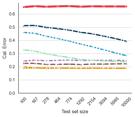
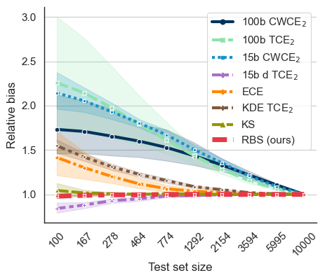
Figure 3: Left: Different calibration error estimates versus the test set size of ResNet Wide 32 and CIFAR100. The red line corresponds to the square root of the Brier score which is an upper bound of the $\text{CE}_{2}$. The other errors are lower bounds. Right: Relative change versus data size with respect to error at full size. Averaging across a multitude of models shows a systematic trend. An unbiased estimator would give a flat line.

In the following, we investigate the behavior of calibration error estimators in three settings.
First, we use varying test set sizes for the estimators and compare their values. This will show how well the inequalities in Theorem 3.1 hold in practical settings and how robust the estimators are. Second, we explore what the estimated improvements of several recalibration methods are. This is done after the recalibration methods are already optimized on a given validation set; we only vary the size of the test set and compute calibration errors on these test sets before and after recalibration. In both settings, the straighter a line is, the more robust and, consequently, trustworthy is the estimator for practical applications. Third, we investigate how our framework can be used to improve calibration for tasks beyond classification by performing probabilistic regression with subsequent recalibration.

In all experiments we evaluate the following estimators: CWCE₂ with 15 equal width bins (’15b CWCE₂’), CWCE₂ with 100 equal width bins (’100b CWCE₂’), ECE with 15 equal width bins (’ECE’), TCE₂ with 100 equal width bins (’100b TCE₂’), TCE₂ with 15 equal mass bins and debias term (’15b d TCE₂’), TCE₂ with kernel density estimation (’KDE TCE₂’), KS (’KS’) and the root calibration upper bound $\sqrt{\mathscr{U}_{\text{BS}}}$ (’RBS (ours)’).The bin amounts are chosen based on past literature [31, 36]. We also evaluate the KDE estimator of CE₁ (’KDE CE₁’) with automatic bandwidth selection based on [43] for CIFAR10. The experiments are conducted across several model-dataset combinations, for which logit sets are openly accessible [29, 45]. This includes the models Wide ResNet 32 [62], DenseNet 40, and DenseNet 161 [22] and the datasets CIFAR10, CIFAR100 [27], and ImageNet [9]. We did not conduct model training ourselves and refer to [29] and [45] for further details. We include TS, ETS, and DIAG as injective recalibration methods. Further details and results on additional models and datasets are reported in the Appendix G.

Robustness of calibration errors to test set size

We illustrate the estimated values of our introduced upper bound and the other errors, which are lower bounds of the unknown CE₂ on the left of Figure 3. On the right, we aggregate across several models to show the systematic drop-off according to Proposition 3.3. The relative bias is computed by $Error(n)/Error(10000)$ and allows an aggregation of models with different calibration levels. Included models are DenseNet 40, Wide ResNet 32, ResNet 110 SD, ResNet 110, and LeNet 5, all trained on CIFAR10. All values represent the calibration of the given model without recalibration transformation. Only our proposed upper bound and KS are stable, and Appendix G shows this holds across a wide range of different settings. The theoretically highest lower bound (CWCE₂ with 100 bins) is also constantly the highest estimated lower bound, but it is sensitive to the test set size. Results for further settings presented in Appendix G show similar results.

Quantifying recalibration improvement

Next, we assessed how well all estimators were able to quantify the improvement in calibration error after applying different injective recalibration methods (Fig. 2). Only our proposed upper bound estimator RBS is again robust throughout all settings. According to Proposition 4.5 and since RBS is asymptotically unbiased and consistent, it can be regarded as a reliable approximation of the real improvement of the presented recalibration methods. For all other estimators, there is a general trend to estimate recalibration improvement higher for large test set sizes. In other settings, especially for small test set sizes, calibration improvement is underestimated to the extent that negative improvements (poorer calibration than before) are suggested. Results on other settings presented in Appendix G show similar results. Taken together, these experiments demonstrate the unreliability of existing calibration estimators, in particular, when used to evaluate recalibration methods. In contrast, our proposed upper bound estimator is stable across different settings.

Variance regression calibration

We consider variance regression to demonstrate the usefulness of proper calibration errors outside the classification setting. To this end, we predict sales prices with an uncertainty estimate in the UCI dataset Residential Building, which consists of a high feature (107) to data instances (372) ratio [44]. Our model of choice is a fully-connected mixture density network predicting mean and variance [2]. Similar to classification, we are interested in recalibration of the predicted variance to adjust possible under- or overconfidence. We use our proposed framework to derive a proper calibration error induced by the proper score DSS for recalibration. Further, we compare DSS [12] to squared KCE (SKCE) [58] and analyze the average predicted variance throughout model training. We use Platt scaling ($x\mapsto wx+b$ with parameters $w,b\in\mathbb{R}$ [42]) on the predicted variance in each training iteration to show how recalibration benefits uncertainty awareness. We expect high uncertainty awareness at the start of the model training with a drop-off at later iterations. As can be seen in Figure 4, recalibration is able to adjust the uncertainty estimate of a model as desired. Further, the DSS estimate, which captures predicted mean and variance correctness, directly communicates the improved variance fit. Contrary, the SKCE estimate appears more erratic between iteration steps and seemingly ignores the changes in variance and the recalibration improvement.

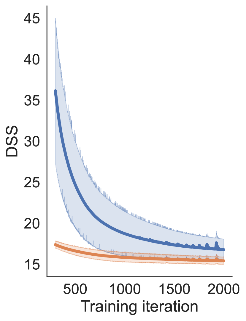
Figure 4: Left: Average predicted variance throughout model training before and after recalibration. Initially, due to a bad fit, recalibration adjusts the variance accordingly for better communicated uncertainty. Once the model fit improves, the predicted variance requires less adjustment due to less uncertainty in each prediction. Middle: DSS communicates reasonably changes in the variance due to recalibration. Right: SKCE fails to capture the variance trend and behaves erratically.

One might also be interested at how the predicted variance corresponds to the mean squared error throughout model training. As we can see in Table 1, only after calibration using a proper calibration error, the average predicted variance (Avg Var) corresponds to the mean squared error.

Table 1: Comparing the mean squared error (MSE) with the average predicted variance (Avg Var) before and after recalibration for various training iterations. Recalibration gives a better average match between prediction and real error.

Iteration	500	750	1000	1250	1500	1750	2000
MSE	10.48	5.87	4.3	3.51	3.12	2.74	2.57
Avg Var (Calibrated)	11.04	6.89	5.4	4.55	4.11	3.63	3.32
Avg Var (Uncalibrated)	0.83	0.83	0.83	0.83	0.83	0.82	0.82

Next, to assess how well the predicted variance corresponds to the instance-level error, we compute the ratio between the squared error of the predictive mean $\mu$ and the predicted variance $\sigma^{2}$ (SE Var Ratio) for each individual sample via $\frac{1}{n}\sum_{i=1}^{n}\frac{\left(\mu_{i}-y_{i}\right)^{2}}{\sigma^{2}_{i}}$.An SE Var Ratio of ’1’ for a given instance means that the predictive uncertainty (variance) exactly matches the squared error, an SE Var Ratio of ’10’ means that the model is overconfident and the squared error is ten times as large as the predicted variance. As we can see in Table 2, recalibration through our framework gives consistently conservative estimates on the squared error, whereas the uncalibrated uncertainties are highly overconfident (with errors more than ten times larger than the prediction).

Table 2: Instance level ratio between the squared error and the predicted variance before and after recalibration for various training iterations. Recalibration improves the instance level prediction of the squared error.

Iteration	500	1000	1500	2000
SE Var Ratio (Calibrated)	0.82 ± 2.17	0.79 ± 2.43	0.79 ± 2.56	0.79 ± 2.59
SE Var Ratio (Uncalibrated)	11.33 ± 30.72	5.36 ± 15.09	4.07 ± 12.13	3.51 ± 11.22

We perform further variance regression experiments in Appendix G.

6 Conclusion

In this work, we address the problem of reliably quantifying the effect of recalibration on predictive uncertainty for classification and other probabilistic tasks. This is critical for adjusting under- or overconfidence via recalibration. To this end, we first provide a taxonomy of existing calibration errors. We discover that most errors are lower bounds of a proper calibration error and fail to assess if a model is calibrated. This motivates our definition of proper calibration errors, which provides a general class of errors for arbitrary probabilistic predictions. Since proper calibration errors cannot be estimated in the general case, we introduce upper bounds, which directly measure the calibration change for injective transformations. This allows us to reliably adjust model uncertainty via recalibration. We demonstrate theoretically and empirically that the estimated calibration improvement can be highly misleading for commonly used estimators, including the ECE. In stark contrast, our upper bound is robust to changes in data size and estimates robustly the improvement via injective recalibration. We further show in additional experiments that our approach can be applied successfully to variance regression.

Appendix A Overview

In this appendix we

• Introduce some notation in section B that we will use throughout the appendix.

• Give rigorous definitions of calibration errors omitted in the main paper in Section C

• Provide proofs for all claims that we make in the main text in Section D.

• Provide details for specific recalibration transformation that illustrate the shortcomings of existing approaches (Section E).

• Give a detailed overview of proper U-scores that can be used to further generalize our proposed framework of proper calibration errors (Section F).

• Give more experimental details and report results from additional experiments (Section G).

Appendix B Notation

The following is implied throughout the appendix. We will use

• The underlying probability space $\left(\Omega,\mathscr{F},\mathbb{P}\right)$, $\mathscr{X}$ the feature space, and $\mathscr{Y}$ the target space.

• Random variables $X\colon\Omega\to\mathscr{X}$ and $Y\colon\Omega\to\mathscr{Y}$.

• $\mathbb{P}_{Y\mid X=x}\left(y\right)\coloneqq\frac{\mathbb{P}\left(\left\{\omega\in\Omega\mid X\left(\omega\right)=x\land Y\left(\omega\right)=y\right\}\right)}{\mathbb{P}\left(\left\{\omega\in\Omega\mid X\left(\omega\right)=x\right\}\right)}$ and $\mathbb{P}_{Y}\left(y\right)\coloneqq\mathbb{P}\left(\left\{\omega\in\Omega\mid Y\left(\omega\right)=y\right\}\right)$ for $x\in\mathscr{X}$ and $y\in\mathscr{Y}$.

• $\mathbb{P}_{Y},\mathbb{P}_{Y\mid X=x}\in\mathscr{P}_{n}$ with $\mathscr{P}_{n}=\left\{p\in\left[0,1\right]^{n}\mid\sum_{k}p_{k}=1\right\}$, and $\mathscr{Y}=\left\{1,\dots,n\right\}$ for categorical $Y$ with $n\in\mathbb{N}$ classes.

• The index ’$-k$’ on a finite vector to denote the removal of index $k$.

• The random variable $C\colon\Omega\to\mathscr{Y}$ defined as $C\coloneqq\arg\max_{k}f_{k}(X)$ for $f\colon\mathscr{X}\to\mathscr{P}_{n}$. It can be regarded as the top-label prediction of $f$.

The notation regarding the (conditional) probability measures will be used for arbitrary random variables.

Appendix C Definitions

A systematic overview of the multitude of calibration errors proposed in the recent literature requires a common notation that can be used to harmonize definitions. For the sake of clarity, we use formulations close to the notation introduced in Kumar et al. [31] and adjust the other errors accordingly, while retaining the notation of the original work whenever possible.

We follow Kumar et al. [31] and define top-label and class-wise calibration errors in expectation:

Definition C.1.

The top-label calibration error of model $f\colon\mathscr{X}\to\mathscr{P}_{n}$ is defined as

$$\text{TCE}_{p}\left(f\right)=\left(\mathbb{E}\left[\left\lvert f_{C}\left(X\right)-\mathbb{P}\left(Y=C\mid f_{C}\left(X\right)\right)\right\rvert^{p}\right]\right)^{\frac{1}{p}}$$

with $C\coloneqq\arg\max_{k}f_{k}\left(X\right)$ and the class-wise calibration error is defined as

$$\text{CWCE}_{p}\left(f\right)=\left(\sum_{k\in\mathscr{Y}}\mathbb{E}\left[\left\lvert f_{k}\left(X\right)-\mathbb{P}\left(Y=k\mid f_{k}\left(X\right)\right)\right\rvert^{p}\right]\right)^{\frac{1}{p}}$$

for $1\leq p\in\mathbb{R}$.

Note that we removed the weighting factors from the original definition in Kumar et al. [31] for easier comparison with the other errors and a fixed upper limit (we will show that CWCE${}_{p}\leq 2^{\frac{1}{p}}$).

Definition C.2.

The Kolmogorov-Smirnov calibration error [16] of model $f\colon\mathscr{X}\to\mathscr{P}_{n}$ is given by

$$\text{KS}\left(f\right)=\mathbb{E}\left[\text{KS}\left(f,C\right)\right],$$

where $C=\arg\max_{k}f_{k}\left(X\right)$ and $\text{KS}\left(f,k\right)=\max_{\sigma\in\left[0,1\right]}\left\lvert\int_{\left[0,\sigma\right]}z-\mathbb{P}\left(Y=k\mid f_{k}\left(X\right)=z\right)\mathrm{d}\mathbb{P}_{f_{k}\left(X\right)}\left(z\right)\right\rvert.$

Definition C.3.

Given a reproducing kernel Hilbert space $\mathscr{H}$ with kernel $k\colon\left[0,1\right]\times\left[0,1\right]\to\mathbb{R}$ the maximum mean calibration error [30] of model $f\colon\mathscr{X}\to\mathscr{P}_{n}$ is

$$\begin{split}&\text{MMCE}\left(f\right)=\\ &\quad\quad\left\|\mathbb{E}\left[\left(f_{C}\left(X\right)-\mathbb{P}\left(Y=C\mid f_{C}\left(X\right)\right)\right)k\left(f_{C}\left(X\right),.\right)\right]\right\|_{\mathscr{H}}.\end{split}$$

Definition C.4.

Given a reproducing kernel Hilbert space $\mathscr{H}$ with kernel $k\colon\mathscr{P}_{n}\times\mathscr{P}_{n}\to\mathbb{R}^{n}\times\mathbb{R}^{n}$ the kernel calibration error [57] of model $f\colon\mathscr{X}\to\mathscr{P}_{n}$ is

$$\begin{split}&\text{KCE}\left(f\right)=\left\|\mathbb{E}\left[\left(f\left(X\right)-\mathbb{P}_{Y\mid f\left(X\right)}\right)k\left(f\left(X\right),.\right)\right]\right\|_{\mathscr{H}}.\end{split}$$

We also need the following score related definitions in the proofs. These are simply a repetition from the main paper.

Definition C.5.

Given a proper score $S$ and $P,Q\in\mathscr{P}$, the expected score $s_{S}\colon\mathscr{P}\times\mathscr{P}\to\mathscr{R}$ is defined as $s_{S}\left(P,Q\right)=\mathbb{E}_{Y\sim Q}\left[S\left(P,Y\right)\right]=\int_{\mathscr{Y}}S\left(P,y\right)\mathrm{d}Q\left(y\right)$.

Definition C.6.

Given a proper score $S$ and $P,Q\in\mathscr{P}$, the associated divergence $d_{S}\colon\mathscr{P}\times\mathscr{P}\to\mathbb{R}_{\geq 0}$ is defined as $d_{S}\left(P,Q\right)=s_{S}\left(P,Q\right)-s_{S}\left(Q,Q\right)$ and the associated generalized entropy $g_{S}\colon\mathscr{P}\to\mathbb{R}$ as $g_{S}\left(Q\right)=s_{S}\left(Q,Q\right)$.

Appendix D Proofs

D.1 Helpers

The following will be of use in several proofs.

Lemma D.1.

Assume that $S$ is a proper score for which CE_S exists, then we have

$$\text{CE}_{S}\left(f\right)=\mathbb{E}\left[S\left(f\left(X\right),Y\right)\right]-\mathbb{E}\left[g_{S}\left(\mathbb{P}_{Y\mid f\left(X\right)}\right)\right].$$

Proof.

$$\begin{split}\text{CE}_{S}\left(f\right)\overset{\text{def }\ref{def:pce}}{}&{=}\mathbb{E}\left[d_{S}\left(f\left(X\right),\mathbb{P}_{Y\mid f\left(X\right)}\right)\right]\\ \overset{\text{def }\ref{def:div_ent}}{}&{=}\mathbb{E}\left[s_{S}\left(f\left(X\right),\mathbb{P}_{Y\mid f\left(X\right)}\right)-s_{S}\left(\mathbb{P}_{Y\mid f\left(X\right)},\mathbb{P}_{Y\mid f\left(X\right)}\right)\right]\\ \overset{\text{def }\ref{def:div_ent}}{}&{=}\mathbb{E}\left[s_{S}\left(f\left(X\right),\mathbb{P}_{Y\mid f\left(X\right)}\right)\right]-\mathbb{E}\left[g_{S}\left(\mathbb{P}_{Y\mid f\left(X\right)}\right)\right]\\ &=\int s_{S}\left(z,\mathbb{P}_{Y\mid f\left(X\right)=z}\right)\mathrm{d}\mathbb{P}_{f\left(X\right)}\left(z\right)-\mathbb{E}\left[g_{S}\left(\mathbb{P}_{Y\mid f\left(X\right)}\right)\right]\\ \overset{\text{def }\ref{def:s_S}}{}&{=}\int\int S\left(z,y\right)\mathrm{d}\mathbb{P}_{Y\mid f\left(X\right)=z}\left(y\right)\mathrm{d}\mathbb{P}_{f\left(X\right)}\left(z\right)-\mathbb{E}\left[g_{S}\left(\mathbb{P}_{Y\mid f\left(X\right)}\right)\right]\\ &=\int S\left(z,y\right)\mathrm{d}\mathbb{P}_{Y,f\left(X\right)}\left(y,z\right)-\mathbb{E}\left[g_{S}\left(\mathbb{P}_{Y\mid f\left(X\right)}\right)\right]\\ &=\mathbb{E}\left[S\left(f\left(X\right),Y\right)\right]-\mathbb{E}\left[g_{S}\left(\mathbb{P}_{Y\mid f\left(X\right)}\right)\right]\\ \end{split}$$ (4)

∎

D.2 Theorem 3.1

Given a model $f\;\colon\;\mathscr{X}\to\mathscr{P}_{n}$ and the above defined errors, we have

$$\begin{split}&\text{BS}\left(f\right)=0\\ \implies&\text{CE}_{p}\left(f\right)=0\\ \iff&\text{KCE}\left(f\right)=0\\ \iff&f\text{ is calibrated}\\ \implies&\text{CWCE}_{p}\left(f\right)=0\\ \implies&\text{TCE}_{p}\left(f\right)=0\\ \iff&\text{MMCE}\left(f\right)=0\\ \iff&\text{KS}\left(f\right)=0\\ \implies&\text{ECE}\left(f\right)=0\\ \end{split}$$ (5)

and

$$\begin{split}n^{\frac{1}{p}-\frac{1}{2}}\sqrt{2}&\geq n^{\frac{1}{p}-\frac{1}{2}}\sqrt{\text{BS}\left(f\right)}\\ \overset{*}{}&{\geq}\text{CE}_{p}\left(f\right)\\ &\geq\text{CWCE}_{p}\left(f\right)\\ &\geq\text{TCE}_{p}\left(f\right)\\ &\geq\text{TCE}_{1}\left(f\right)\\ &\geq\begin{cases}\text{KS}\left(f\right)\\ \text{ECE}\left(f\right)\\ c\cdot\text{MMCE}\left(f\right)\end{cases}\geq 0\end{split}$$ (6)

for $1\leq p\in\mathbb{R}$. * BS is only included for $p\leq 2$. We define $c=\sqrt{\max_{r}k\left(r,r\right)}$ as given in Theorem 3 of Kumar et al. [30].

Proof.

Regarding BS$\left(f\right)=0\implies$ CE${}_{p}\left(f\right)=0\iff\text{KCE}\left(f\right)=0\iff f\text{ is calibrated}$:

$$\begin{split}\text{BS}\left(f\right)=0&\iff\mathbb{P}_{Y\mid X}\overset{\text{a.s.}}{=}f\left(X\right)\\ &\implies\mathbb{P}_{Y\mid f\left(X\right)}\overset{\text{a.s.}}{=}f\left(X\right)\\ &\iff\begin{cases}\text{CE}_{p}\left(f\right)=0\\ \text{KCE}\left(f\right)=0\\ f\text{ is calibrated}\end{cases}\end{split}$$ (7)

The last equivalence follows from Definition 2.1 and 2, and according to Widmann et al. [57]. Since the equivalence in the last line holds for each, it follows CE${}_{p}\left(f\right)=0\iff\text{KCE}\left(f\right)=0\iff f\text{ is calibrated}$. Example sketch for BS$\left(f\right)=0\centernot\impliedby$ CE${}_{p}\left(f\right)=0$: Set $f\left(.\right)=\mathbb{P}_{Y}$, then $f\left(X\right)=\mathbb{P}_{Y}=\mathbb{P}_{Y\mid\mathbb{P}_{Y}}=\mathbb{P}_{Y\mid f\left(X\right)}$, but BS$\left(f\right)>0$.

Regarding CE${}_{p}\left(f\right)=0\implies$ CWCE${}_{p}\left(f\right)=0$:

$$\begin{split}\text{CE}_{p}\left(f\right)=0&\iff\mathbb{P}_{Y\mid f\left(X\right)}\overset{\text{a.s.}}{=}f\left(X\right)\\ &\iff\mathbb{P}\left(Y=k\mid f\left(X\right)\right)\overset{\text{a.s.}}{=}f_{k}\left(X\right)\quad\forall k\\ &\implies\mathbb{E}_{f_{-k}\left(X\right)}\left[\mathbb{P}\left(Y=k\mid f\left(X\right)\right)\mid f_{k}\left(X\right)\right]\overset{\text{a.s.}}{=}\mathbb{E}_{f_{-k}}\left[f_{k}\left(X\right)\mid f_{k}\left(X\right)\right]\quad\forall k\\ &\iff\mathbb{P}\left(Y=k\mid f_{k}\left(X\right)\right)\mid f_{k}\left(X\right)\overset{\text{a.s.}}{=}f_{k}\left(X\right)\quad\forall k\\ &\iff\sum_{k\in\mathscr{Y}}\mathbb{E}\left[\left(\mathbb{P}\left(Y=k\mid f_{k}\left(X\right)\right)-f_{k}\left(X\right)\right)^{p}\right]=0\\ &\iff\text{CWCE}_{p}\left(f\right)=0\end{split}$$ (8)

An example for CE${}_{p}\left(f\right)=0\centernot\impliedby$ CWCE${}_{p}\left(f\right)=0$ is given in the proof of Proposition 3.2 located in Appendix D.3.

Regarding CWCE${}_{p}\left(f\right)=0\implies$ TCE${}_{p}\left(f\right)=0\iff\text{MMCE}\left(f\right)=0$:

$$\begin{split}\text{CWCE}_{p}\left(f\right)=0&\iff\mathbb{P}\left(Y=k\mid f_{k}\left(X\right)\right)\overset{\text{a.s.}}{=}f_{k}\left(X\right)\quad\forall k\\ &\implies\mathbb{P}\left(Y=C\mid f_{C}\left(X\right)\right)\overset{\text{a.s.}}{=}f_{C}\left(X\right)\\ &\iff\mathbb{P}\left(Y=\arg\max_{k}f_{k}\left(X\right)\mid\max_{k}f_{k}\left(X\right)\right)\overset{\text{a.s.}}{=}\max_{k}f_{k}\left(X\right)\\ &\iff\begin{cases}\text{TCE}_{p}\left(f\right)=0\\ \text{MMCE}\left(f\right)=0\end{cases}\end{split}$$ (9)

See Theorem 1 in Kumar et al. [30] regarding MMCE. Note that we could not verify their claim that MMCE is a proper score, which is even contradictive to our findings. A sketch for an example where CWCE${}_{p}\left(f\right)=0\centernot\impliedby$ TCE${}_{p}\left(f\right)=0$ is if $\mathbb{P}\left(Y=C\mid f_{C}\left(X\right)\right)\overset{\text{a.s.}}{=}f_{C}\left(X\right)$ and $\mathbb{P}\left(Y=\arg\min_{k}f_{k}\left(X\right)\mid\min_{k}f_{k}\left(X\right)\right)\neq\min_{k}f_{k}\left(X\right)$.

Regarding TCE${}_{p}\left(f\right)=0\iff\text{KS}\left(f\right)=0$:

$$\begin{split}&\text{TCE}_{p}\left(f\right)=0\\ &\iff\mathbb{P}\left(Y=\arg\max_{k}f_{k}\left(X\right)\mid\max_{l}f_{l}\left(X\right)\right)\overset{\text{a.s.}}{=}\max_{m}f_{m}\left(X\right)\\ &\iff\mathbb{P}\left(Y=C\mid f_{C}\left(X\right)\right)\overset{\text{a.s.}}{=}f_{C}\left(X\right)\\ \overset{(i)}{}&{\iff}\int_{\sigma^{\prime}}\mathbb{P}\left(Y=C\mid f_{C}\left(X\right)=z\right)\mathrm{d}\mathbb{P}_{f_{C}\left(X\right)\mid C}\left(z\right)\overset{\text{a.s.}}{=}\int_{\sigma^{\prime}}z\mathrm{d}\mathbb{P}_{f_{C}\left(X\right)\mid C}\left(z\right),\quad\forall\sigma^{\prime}\subset\left[0,1\right]\\ &\iff\int_{\left[0,\sigma\right]}\mathbb{P}\left(Y=C\mid f_{C}\left(X\right)=z\right)\mathrm{d}\mathbb{P}_{f_{C}\left(X\right)\mid C}\left(z\right)\overset{\text{a.s.}}{=}\int_{\left[0,\sigma\right]}z\mathrm{d}\mathbb{P}_{f_{C}\left(X\right)\mid C}\left(z\right),\quad\forall\sigma\in\left[0,1\right]\\ &\iff\mathbb{E}\left[\max_{\sigma\in\left[0,1\right]}\left\lvert\int_{\left[0,\sigma\right]}z-\mathbb{P}\left(Y=C\mid f_{C}\left(X\right)=z\right)\mathrm{d}\mathbb{P}_{f_{C}\left(X\right)\mid C}\left(z\right)\right\rvert\right]=0\\ &\iff\mathbb{E}\left[\text{KS}\left(f,C\right)\right]=0\\ &\iff\text{KS}\left(f\right)=0\\ \end{split}$$ (10)

(i) according to Theorem 4.22 of Capiński & Kopp [5].

Regarding TCE${}_{p}\left(f\right)=0\implies\text{ECE}\left(f\right)=0$:

$$\begin{split}&\text{TCE}_{p}\left(f\right)=0\\ &\iff\mathbb{P}\left(Y=C\mid f_{C}\left(X\right)\right)\overset{\text{a.s.}}{=}f_{C}\left(X\right)\\ \overset{\text{(i)}}{}&{\implies}\forall i=1,\dots,m\colon\;\mathbb{P}\left(Y=C\mid f_{C}\left(X\right)\in B_{i}\right)\overset{\text{a.s.}}{=}\mathbb{E}\left[f_{C}\left(X\right)\mid f_{C}\left(X\right)\in B_{i}\right]\\ \overset{\text{def }\ref{def:ece}}{}&{\iff}\text{ECE}\left(f\right)=0\end{split}$$ (11)

(i) with $B_{i}$ defined as in definition 3; follows since $\mathbb{P}\left(Y=C\mid f_{C}\left(X\right)\in B_{i}\right)=\int_{B_{i}}\mathbb{P}\left(Y=C\mid f_{C}\left(X\right)=z\right)\mathrm{d}\mathbb{P}_{f_{C}\left(X\right)}\left(z\right)\overset{\text{a.s.}}{=}\int_{B_{i}}f_{C}\left(X\right)\mathrm{d}\mathbb{P}_{f_{C}\left(X\right)}\left(z\right)=\mathbb{E}\left[f_{C}\left(X\right)\mid f_{C}\left(X\right)\in B_{i}\right]$.

An intuition of why TCE${}_{1}\left(f\right)=0\centernot\impliedby\text{ECE}\left(f\right)=0$ is given in example 3.2 of Kumar et al. [31].

Regarding $2\geq\text{BS}\left(f\right)\geq\left(\text{CE}_{2}\left(f\right)\right)^{2}$:

$$\begin{split}&2=\left\|e_{1}-e_{2}\right\|^{2}_{2}\\ &\geq\mathbb{E}\left[\left\|f\left(X\right)-e_{Y}\right\|^{2}_{2}\right]\\ \overset{\text{def }\ref{def:bs}}{}&{=}\text{BS}\left(f\right)\\ \overset{\text{(i)}}{}&{\geq}\text{BS}\left(f\right)-\mathbb{E}\left[g_{\text{BS}}\left(\mathbb{P}_{Y\mid f\left(X\right)}\right)\right]\\ \overset{\text{le }\ref{le:cal_decomp}}{}&{=}\text{CE}_{\text{BS}}\left(f\right)\\ \overset{\text{(ii)}}{}&{=}\left(\text{CE}_{2}\left(f\right)\right)^{2}\\ \end{split}$$ (12)

(i) $g_{\text{BS}}$ non-negative, follows from definition C.6.
(ii) compare definition 2 with the squared calibration term in [38].

Regarding $n^{\frac{1}{p}-\frac{1}{q}}\text{CE}_{q}\left(f\right)\geq\text{CE}_{p}\left(f\right)$ for $0<p\leq q<\infty$:

We use $\Delta\coloneqq f\left(X\right)-\mathbb{P}_{Y\mid f\left(X\right)}$ for shorter equations. Further, we use the $p$-norm inequality $n^{\frac{1}{p}-\frac{1}{q}}\left\|x\right\|_{q}\geq\left\|x\right\|_{p}$ for a vector $x\in\mathbb{R}^{n}$ and the $L^{p}$ space inequality $\left(\mathbb{E}\left[\left\lvert X\right\rvert^{q}\right]\right)^{\frac{1}{q}}\geq\left(\mathbb{E}\left[\left\lvert X\right\rvert^{p}\right]\right)^{\frac{1}{p}}$ for $X\in L^{q}\subset L^{p}$ [5].

$$\begin{split}&\text{CE}_{p}\left(f\right)\\ \overset{\text{def }\ref{def:lp_ce}}{=}&\left(\mathbb{E}\left[\left\|\Delta\right\|^{p}_{p}\right]\right)^{\frac{1}{p}}\\ \leq&\left(\mathbb{E}\left[\left(n^{\frac{1}{p}-\frac{1}{q}}\left\|\Delta\right\|_{q}\right)^{p}\right]\right)^{\frac{1}{p}}\\ =&n^{\frac{1}{p}-\frac{1}{q}}\left(\mathbb{E}\left[\left\|\Delta\right\|_{q}^{p}\right]\right)^{\frac{1}{p}}\\ \leq&n^{\frac{1}{p}-\frac{1}{q}}\left(\mathbb{E}\left[\left\|\Delta\right\|_{q}^{q}\right]\right)^{\frac{1}{q}}\\ \overset{\text{def }\ref{def:lp_ce}}{=}&n^{\frac{1}{p}-\frac{1}{q}}\text{CE}_{q}\left(f\right)\\ \end{split}$$ (13)

Note that this result is a direct contradiction to Theorem 1 of [56] since $n^{\frac{1}{p}-\frac{1}{q}}>1$.

Further, the name ’$L^{p}$ calibration error’ is unambiguous for canonical calibration since the following holds. Let $\left\lVert.\right\rVert_{\mathbb{R}^{n},p}$ be the vector $p$-norm and $\left\lVert.\right\rVert_{L^{p}}$ the norm of the $L^{p}$ space. Then we have

$$\text{CE}_{p}\left(f\right)=\left\lVert\left\lVert\Delta\right\rVert_{\mathbb{R}^{n},p}\right\rVert_{L^{p}}=\left\lVert\left(\left\lVert\Delta_{1}\right\rVert_{L^{p}},\dots,\left\lVert\Delta_{n}\right\rVert_{L^{p}}\right)^{\intercal}\right\rVert_{\mathbb{R}^{n},p}.$$ (14)

Thus, there is no ambiguity if we first compute the vector norm or the $L^{p}$ norm and there cannot be another $L^{p}$ calibration error with a different norm order.

Regarding $n^{\frac{1}{p}-\frac{1}{2}}\sqrt{\text{BS}\left(f\right)}\geq\text{CE}_{p}\left(f\right)$ for $0<p\leq 2$:

Combining equations (LABEL:eq:BS>CE22) and (LABEL:eq:CEq<CEp) (with $q=2$) gives the result.

Regarding $\text{CE}_{p}\left(f\right)\geq\text{CWCE}_{p}\left(f\right)$:

In the following, we will use Tonelli’s theorem to split the expectation into two and the Jensen’s inequality for the convex function $\lvert.\rvert^{p}$.

$$\begin{split}\left(\text{CE}_{p}\left(f\right)\right)^{p}&=\mathbb{E}\left[\left\|f\left(X\right)-\mathbb{P}_{Y\mid f\left(X\right)}\right\|^{p}_{p}\right]\\ &=\sum_{k\in\mathscr{Y}}\mathbb{E}\left[\left\lvert f_{k}\left(X\right)-\mathbb{P}\left(Y=k\mid f\left(X\right)\right)\right\rvert^{p}\right]\\ \overset{\text{Tonelli}}{}&{=}\sum_{k\in\mathscr{Y}}\mathbb{E}_{f_{k}\left(X\right)}\left[\mathbb{E}_{f_{-k}\left(X\right)}\left[\left\lvert f_{k}\left(X\right)-\mathbb{P}\left(Y=k\mid f\left(X\right)\right)\right\rvert^{p}\mid f_{k}\left(X\right)\right]\right]\\ \overset{\text{Jensen}}{}&{\geq}\sum_{k\in\mathscr{Y}}\mathbb{E}_{f_{k}\left(X\right)}\left[\left\lvert\mathbb{E}_{f_{-k}\left(X\right)}\left[f_{k}\left(X\right)-\mathbb{P}\left(Y=k\mid f\left(X\right)\right)\mid f_{k}\left(X\right)\right]\right\rvert^{p}\right]\\ &=\sum_{k\in\mathscr{Y}}\mathbb{E}_{f_{k}\left(X\right)}\left[\left\lvert f_{k}\left(X\right)-\mathbb{P}\left(Y=k\mid f_{k}\left(X\right)\right)\right\rvert^{p}\right]\\ \overset{\text{def }\ref{def:cw_tce}}{}&{=}\left(\text{CWCE}_{p}\left(f\right)\right)^{p}\end{split}$$ (15)

Regarding $\text{CWCE}_{p}\left(f\right)\geq\text{TCE}_{p}\left(f\right)$:

We will use $F\coloneqq f\left(X\right)$ for shorter notation.

$$\begin{split}\left(\text{CWCE}_{p}\left(f\right)\right)^{p}\overset{\text{def }\ref{def:cw_tce}}{}&{=}\sum_{k\in\mathscr{Y}}\mathbb{E}_{f_{k}\left(X\right)}\left[\left\lvert f_{k}\left(X\right)-\mathbb{P}\left(Y=k\mid f_{k}\left(X\right)\right)\right\rvert^{p}\right]\\ &=\sum_{k\in\mathscr{Y}}\mathbb{E}_{F_{k}}\left[\left\lvert F_{k}-\mathbb{P}\left(Y=k\mid F_{k}\right)\right\rvert^{p}\right]\\ &=\sum_{k\in\mathscr{Y}}\mathbb{E}_{F}\left[\left\lvert F_{k}-\mathbb{P}\left(Y=k\mid F_{k}\right)\right\rvert^{p}\right]\\ &=\mathbb{E}_{F}\left[\sum_{k\in\mathscr{Y}}\left\lvert F_{k}-\mathbb{P}\left(Y=k\mid F_{k}\right)\right\rvert^{p}\right]\\ \overset{\text{(i)}}{}&{=}\mathbb{E}_{F}\left[\sum_{k\in\mathscr{Y}}\left\lvert F_{\left(k\right)_{F}}-\mathbb{P}\left(Y=\left(k\right)_{F}\mid F_{\left(k\right)_{F}}\right)\right\rvert^{p}\right]\\ &\geq\mathbb{E}_{F}\left[\left\lvert F_{\left(1\right)_{F}}-\mathbb{P}\left(Y=\left(1\right)_{F}\mid F_{\left(1\right)_{F}}\right)\right\rvert^{p}\right]\\ \overset{\text{(ii)}}{}&{=}\mathbb{E}_{F}\left[\left\lvert F_{C}-\mathbb{P}\left(Y=C\mid F_{C}\right)\right\rvert^{p}\right]\\ &=\mathbb{E}_{f\left(X\right)}\left[\left\lvert f_{C}\left(X\right)-\mathbb{P}\left(Y=C\mid f_{C}\left(X\right)\right)\right\rvert^{p}\right]\\ \overset{\text{def }\ref{def:cw_tce}}{}&{=}\left(\text{TCE}_{p}\left(f\right)\right)^{p}\end{split}$$ (16)

(i) Order all summands by $F$. We use notation of order statistics to refer to $\left(k\right)_{F}$ the index with the $k$th highest rank according to $F$.
(ii) From (i) follows $\left(1\right)_{F}=\left(1\right)_{f\left(X\right)}=\arg\max_{k}f_{k}\left(X\right)=C$.

Regarding $\text{TCE}_{p}\left(f\right)\geq\text{TCE}_{1}\left(f\right)$:

Let $p\geq q\geq 1$. This makes $\left(.\right)^{\frac{p}{q}}$ a convex function for positive arguments. We will show the more general $\text{TCE}_{p}\left(f\right)\geq\text{TCE}_{q}\left(f\right)$. From this directly follows $\text{TCE}_{p}\left(f\right)\geq\text{TCE}_{1}\left(f\right)$.

$$\begin{split}&\text{TCE}_{p}\left(f\right)\\ &=\left(\mathbb{E}\left[\left\lvert f_{C}\left(X\right)-\mathbb{P}\left(Y=C\mid f_{C}\left(X\right)\right)\right\rvert^{p}\right]\right)^{\frac{1}{p}}\\ &=\left(\mathbb{E}\left[\left\lvert f_{C}\left(X\right)-\mathbb{P}\left(Y=C\mid f_{C}\left(X\right)\right)\right\rvert^{q\frac{p}{q}}\right]\right)^{\frac{1}{p}}\\ \overset{\text{Jensen}}{}&{\geq}\left(\mathbb{E}\left[\left\lvert f_{C}\left(X\right)-\mathbb{P}\left(Y=C\mid f_{C}\left(X\right)\right)\right\rvert^{q}\right]\right)^{\frac{1}{p}\frac{p}{q}}\\ &=\left(\mathbb{E}\left[\left\lvert f_{C}\left(X\right)-\mathbb{P}\left(Y=C\mid f_{C}\left(X\right)\right)\right\rvert^{q}\right]\right)^{\frac{1}{q}}\\ &=\text{TCE}_{q}\left(f\right)\\ \end{split}$$ (17)

Regarding $\text{TCE}_{1}\left(f\right)\geq\text{KS}\left(f\right)$:

We will show the more general $\text{TCE}_{p}\left(f\right)\geq\text{KS}\left(f\right)$, from which $\text{TCE}_{1}\left(f\right)\geq\text{KS}\left(f\right)$ follows.

We will make use of the indicator function for a set $A$ defined as $\mathbbm{1}_{A}\left(a\right)=\begin{cases}1,&a\in A\\ 0,&\text{ else.}\end{cases}$

$$\begin{split}\left(\text{TCE}_{p}\left(f\right)\right)^{p}&=\mathbb{E}\left[\left\lvert f_{C}\left(X\right)-\mathbb{P}\left(Y=C\mid f_{C}\left(X\right)\right)\right\rvert^{p}\right]\\ \overset{\text{Tonelli}}{}&{=}\mathbb{E}_{C}\left[\mathbb{E}_{f_{C}\left(X\right)}\left[\left\lvert f_{C}\left(X\right)-\mathbb{P}\left(Y=C\mid f_{C}\left(X\right)\right)\right\rvert^{p}\mid C\right]\right]\\ &=\mathbb{E}_{C}\left[\mathbb{E}_{f_{C}\left(X\right)}\left[\mathbbm{1}_{\left[0,1\right]}\left(f_{C}\left(X\right)\right)\left\lvert f_{C}\left(X\right)-\mathbb{P}\left(Y=C\mid f_{C}\left(X\right)\right)\right\rvert^{p}\mid C\right]\right]\\ \overset{\text{(i)}}{}&{=}\mathbb{E}_{C}\left[\max_{\sigma\in\left[0,1\right]}\mathbb{E}_{f_{C}\left(X\right)}\left[\mathbbm{1}_{\left[0,\sigma\right]}\left(f_{C}\left(X\right)\right)\left\lvert f_{C}\left(X\right)-\mathbb{P}\left(Y=C\mid f_{C}\left(X\right)\right)\right\rvert^{p}\mid C\right]\right]\\ &=\mathbb{E}_{C}\left[\max_{\sigma\in\left[0,1\right]}\mathbb{E}_{f_{C}\left(X\right)}\left[\left\lvert\mathbbm{1}_{\left[0,\sigma\right]}\left(f_{C}\left(X\right)\right)\left(f_{C}\left(X\right)-\mathbb{P}\left(Y=C\mid f_{C}\left(X\right)\right)\right)\right\rvert^{p}\mid C\right]\right]\\ \overset{\text{Jensen}}{}&{\geq}\mathbb{E}_{C}\left[\max_{\sigma\in\left[0,1\right]}\left\lvert\mathbb{E}_{f_{C}\left(X\right)}\left[\mathbbm{1}_{\left[0,\sigma\right]}\left(f_{C}\left(X\right)\right)\left(f_{C}\left(X\right)-\mathbb{P}\left(Y=C\mid f_{C}\left(X\right)\right)\right)\mid C\right]\right\rvert^{p}\right]\\ &=\mathbb{E}_{C}\left[\max_{\sigma\in\left[0,1\right]}\left\lvert\int_{\left[0,1\right]}\mathbbm{1}_{\left[0,\sigma\right]}\left(z\right)\left(z-\mathbb{P}\left(Y=C\mid f_{C}\left(X\right)=z\right)\right)\mathrm{d}\mathbb{P}_{f_{C}\left(X\right)\mid C}\left(z\right)\right\rvert^{p}\right]\\ &=\mathbb{E}_{C}\left[\max_{\sigma\in\left[0,1\right]}\left\lvert\int_{\left[0,\sigma\right]}z-\mathbb{P}\left(Y=C\mid f_{C}\left(X\right)=z\right)\mathrm{d}\mathbb{P}_{f_{C}\left(X\right)\mid C}\left(z\right)\right\rvert^{p}\right]\\ \overset{\text{Jensen}}{}&{\geq}\left(\mathbb{E}_{C}\left[\max_{\sigma\in\left[0,1\right]}\left\lvert\int_{\left[0,\sigma\right]}z-\mathbb{P}\left(Y=C\mid f_{C}\left(X\right)=z\right)\mathrm{d}\mathbb{P}_{f_{C}\left(X\right)\mid C}\left(z\right)\right\rvert\right]\right)^{p}\\ \overset{\text{def }\ref{def:ks_error}}{}&{=}\left(\mathbb{E}_{C}\left[\text{KS}\left(f,C\right)\right]\right)^{p}\\ \overset{\text{def }\ref{def:ks_error}}{}&{=}\left(\text{KS}\left(f\right)\right)^{p}\end{split}$$ (18)

(i) $\sigma\geq\sigma^{\prime}\implies\mathbbm{1}_{\left[0,\sigma\right]}\left(f_{C}\left(X\right)\right)\left\lvert f_{C}\left(X\right)-\mathbb{P}\left(Y=C\mid f_{C}\left(X\right)\right)\right\rvert^{p}\geq\mathbbm{1}_{\left[0,\sigma^{\prime}\right]}\left(f_{C}\left(X\right)\right)\left\lvert f_{C}\left(X\right)-\mathbb{P}\left(Y=C\mid f_{C}\left(X\right)\right)\right\rvert^{p}\geq 0$.

Regarding $\text{TCE}_{1}\left(f\right)\geq c\cdot\text{MMCE}\left(f\right)$:

This is given in the proof of Theorem 3 of Kumar et al. [30]. Note that Kumar et al. [30] used ECE in their theorem, but their proof is actually given for TCE₁. Since ECE$\left(f\right)=0\centernot\implies\text{MMCE}\left(f\right)=0$, we have $\text{ECE}\left(f\right)\centernot\geq c\cdot\text{MMCE}\left(f\right)$.

Regarding $\text{TCE}_{1}\left(f\right)\geq\text{ECE}\left(f\right)$:

A similar statement for binary models is given in Proposition 3.3 of Kumar et al. [31] or for general models in Theorem 2 of Vaicenavicius et al. [53]. Since our formulations differ, we provide an independent proof.

We will write $B_{i}\coloneqq\left(\frac{i-1}{m},\frac{i}{m}\right]$. Let $\mathscr{B}\coloneqq\sigma\left(\left\{B_{1},\dots,B_{m}\right\}\right)$ be the $\sigma$-algebra generated by the binning scheme of size $m\in\mathbb{N}$ used for the ECE.

$$\begin{split}\text{TCE}_{1}\left(f\right)&=\mathbb{E}\left[\left\lvert f_{C}\left(X\right)-\mathbb{P}\left(Y=C\mid f_{C}\left(X\right)\right)\right\rvert\right]\\ &=\mathbb{E}\left[\mathbb{E}\left[\left\lvert f_{C}\left(X\right)-\mathbb{P}\left(Y=C\mid f_{C}\left(X\right)\right)\right\rvert\mid\mathscr{B}\right]\right]\\ \overset{\text{(i)}}{}&{\geq}\mathbb{E}\left[\left\lvert\mathbb{E}\left[f_{C}\left(X\right)-\mathbb{P}\left(Y=C\mid f_{C}\left(X\right)\right)\mid\mathscr{B}\right]\right\rvert\right]\\ &=\mathbb{E}\left[\left\lvert\mathbb{E}\left[f_{C}\left(X\right)\mid\mathscr{B}\right]-\mathbb{P}\left(Y=C\mid\mathbb{E}\left[f_{C}\left(X\right)\mid\mathscr{B}\right]\right)\right\rvert\right]\\ &=\sum_{i=1}^{m}\mathbb{P}\left(f\left(X\right)\in B_{i}\right)\cdot\\ &\quad\quad\left\lvert\mathbb{E}\left[f_{C}\left(X\right)\mid f\left(X\right)\in B_{i}\right]-\mathbb{P}\left(Y=C\mid f\left(X\right)\in B_{i}\right)\right\rvert\\ \overset{\text{def }\ref{def:ece}}{}&{=}\text{ECE}\left(f\right)\\ \end{split}$$ (19)

(i) We use conditional Jensen’s inequality [5].

∎

D.3 Proposition 3.2

For all $\epsilon>0$ and surjective $f\colon\mathscr{X}\to\mathscr{P}_{n}$ there exists a joint distribution $\mathbb{P}_{X,Y}$ such that for all $E\in\left\{\text{MMCE},\text{KS},\text{ECE},\text{TCE}_{p},\text{CWCE}_{p}\mid 1\leq p\in\mathbb{R}\right\}\colon$

$$\begin{split}E\left(f\right)=0\quad\land\quad\text{CE}_{2}\left(f\right)\geq 1-\frac{1}{n}-\epsilon.\end{split}$$

Proof.

Assume arbitrary $\epsilon>0$ and surjective $f\colon\mathscr{X}\to\mathbb{P}_{n}$. Choose $\mathbb{P}_{X,Y}$ such that $\mathbb{E}\left[\left\|f\left(X\right)\right\|^{2}_{2}\right]\leq\frac{1}{n}+\epsilon$ and

$$\mathbb{P}\left(Y=k\mid f\left(X\right)\right)=\begin{cases}1&\text{, with probability $f_{k}\left(X\right)$}\\ 0&\text{, else.}\\ \end{cases}$$

This is possible, since $\|.\|^{2}_{2}\colon\mathscr{P}_{n}\to\left[\frac{1}{n},1\right]$ and $f$ are surjective, from which folows $\forall\epsilon>0\;\exists x\in\mathscr{X}\colon\quad\frac{1}{n}+\epsilon\geq\left\|f\left(x\right)\right\|^{2}_{2}$.

Write $F\coloneqq f\left(X\right)$ and $\mathbf{Y}\coloneqq e_{Y}$ (one-hot encoded $Y$).

Then we have $\mathbb{P}\left(Y=k\mid F_{k}\right)=\mathbb{E}\left[\mathbf{Y}_{k}\mid F_{k}\right]=\mathbb{E}_{F_{-k}}\left[\mathbb{E}\left[\mathbf{Y}_{k}\mid F\right]\mid F_{k}\right]=F_{k}$ and consequently $\text{CWCE}_{p}\left(f\right)=0$. The other errors follow from Theorem 3.1. But we also have

$$\begin{split}\left(\text{CE}_{2}\left(f\right)\right)^{2}&=\mathbb{E}\left[\left\|\mathbb{P}_{Y\mid f\left(X\right)}-f\left(X\right)\right\|^{2}_{2}\right]\\ &=\mathbb{E}\left[\left\|\mathbb{E}\left[\mathbf{Y}\mid F\right]-F\right\|^{2}_{2}\right]\\ &=\sum_{k\in\mathscr{Y}}\mathbb{E}\left[\left(\mathbb{E}\left[\mathbf{Y}_{k}\mid F\right]-F_{k}\right)^{2}\right]\\ &=\sum_{k\in\mathscr{Y}}\mathbb{E}\left[\left(\mathbb{E}\left[\mathbf{Y}_{k}\mid F\right]\right)^{2}\right]-2\mathbb{E}\left[\mathbb{E}\left[\mathbf{Y}_{k}\mid F\right]F_{k}\right]+\mathbb{E}\left[F_{k}^{2}\right]\\ &=\sum_{k\in\mathscr{Y}}\mathbb{E}\left[\mathbb{E}\left[\mathbf{Y}_{k}\mid F\right]\right]-2\mathbb{E}\left[\mathbb{E}\left[\mathbf{Y}_{k}\mid F\right]F_{k}\right]+\mathbb{E}\left[F_{k}^{2}\right]\\ &=1-2\sum_{k\in\mathscr{Y}}\mathbb{E}\left[\mathbb{E}\left[\mathbf{Y}_{k}\mid F\right]F_{k}\right]+\sum_{k\in\mathscr{Y}}\mathbb{E}\left[F_{k}^{2}\right]\\ &=1-2\sum_{k\in\mathscr{Y}}\mathbb{E}\left[\mathbb{E}\left[\mathbf{Y}_{k}\mid F_{k}\right]F_{k}\right]+\sum_{k\in\mathscr{Y}}\mathbb{E}\left[F_{k}^{2}\right]\\ &=1-2\sum_{k\in\mathscr{Y}}\mathbb{E}\left[F_{k}^{2}\right]+\sum_{k\in\mathscr{Y}}\mathbb{E}\left[F_{k}^{2}\right]\\ &=1-\sum_{k\in\mathscr{Y}}\mathbb{E}\left[F_{k}^{2}\right]\\ &=1-\mathbb{E}\left[\left\|F\right\|^{2}_{2}\right]\\ &\geq 1-\frac{1}{n}-\epsilon\end{split}$$ (20)

∎

D.4 Proposition D.2

Proposition 3.2 tells us about the existence of settings such that common errors are insufficient to capture miscalibration. We might still wonder how likely it is to encounter such a situation in practice. Indeed, we can come up with a recalibration transformation that is perfect according to these errors and accuracy-preserving but not calibrated. For this, assume that $f\colon\mathscr{X}\to\mathscr{P}_{n}$ is a trained model. Define $t^{f}\colon\mathscr{P}_{n}\to\mathscr{P}_{n}$ to replace the largest entry in its input with the accuracy of model $f$. The other entries are set such that the output is a unit vector. A more formal definition is provided in the proof.

Proposition D.2.

For all models $f\colon\mathscr{X}\to\mathscr{P}_{n}$ and $E\in\left\{\text{MMCE},\text{KS},\text{ECE},\text{TCE}_{p}\mid 1\leq p\in\mathbb{R}\right\}$ we have

$$\begin{split}E\left(t^{f}\circ f\right)=0\quad\text{and}\quad\text{ACC}\left(t^{f}\circ f\right)=\text{ACC}\left(f\right).\end{split}$$

But, $t^{f}\circ f$ is not calibrated in general.

Proof.

Assume we are given a model $f\colon\mathscr{X}\to\mathscr{P}_{n}$.

Define $\sigma\colon\mathscr{P}_{n}\times\mathscr{P}_{n}\to\mathscr{P}_{n}$ to order the entries of its second input according to the values given in the first input. Let $\sigma^{-1}\colon\mathscr{P}_{n}\times\mathscr{P}_{n}\to\mathscr{P}_{n}$ revert the ordering in the second input according to the entries of its first input. For easier notation, we will write $\sigma_{u}\left(v\right)\coloneqq\sigma\left(u,v\right)$ and $\sigma^{-1}_{u}\left(v\right)\coloneqq\sigma^{-1}\left(u,v\right)$, which gives $\forall u,v\in\mathscr{P}\colon\;\sigma^{-1}_{u}\circ\sigma_{u}\left(v\right)=v$. I.e. $\sigma^{-1}_{u}$ is the inverse of $\sigma_{u}$ given $u$.

Define $c_{f}\coloneqq\left(\text{ACC}\left(f\right),\frac{1-\text{ACC}\left(f\right)}{n-1},\dots,\frac{1-\text{ACC}\left(f\right)}{n-1}\right)^{\intercal}\in\mathscr{P}_{n}$.

Now, we can give a formal definition of $t^{f}$, which is defined as $t^{f}\left(p\right)=\sigma^{-1}_{p}\left(c_{f}\right)$.

Regarding accuracy:

We will use $[.]_{k}$ to denote entry with index $k$ of the expression inside the brackets. Since we can assume $\text{ACC}\left(f\right)>\frac{1-\text{ACC}\left(f\right)}{n-1}$ in every practical setting, we have

$$\begin{split}&\arg\max_{k}t^{f}_{k}\circ f\left(X\right)\\ &=\arg\max_{k}\left[\sigma^{-1}_{f\left(X\right)}\left(c_{f}\right)\right]_{k}\\ \overset{(i)}{}&{=}\arg\max_{k}\left[\sigma^{-1}_{f\left(X\right)}\circ\sigma_{f\left(X\right)}\left(f\left(X\right)\right)\right]_{k}\\ &=\arg\max_{k}\left[f\left(X\right)\right]_{k}\\ &=\arg\max_{k}f_{k}\left(X\right).\end{split}$$ (21)

(i) $c_{f}$ and $\sigma_{f\left(X\right)}\left(f\left(X\right)\right)$ have their largest entry at index $k=1$.

This states that $t^{f}$ is accuracy-preserving.

Regarding zero TCE:

Note that ACC$\left(f\right)=\mathbb{P}\left(Y=\arg\max_{k}f_{k}\left(X\right)\right)$. Using this, we have $\mathbb{P}\left(Y=\arg\max_{k}t^{f}_{k}\circ f\left(X\right)\mid\max_{k}t^{f}_{k}\circ f\left(X\right)\right)=\mathbb{P}\left(Y=\arg\max_{k}f_{k}\left(X\right)\mid\text{ACC}\left(f\right)\right)=\mathbb{P}\left(Y=\arg\max_{k}f_{k}\left(X\right)\right)=\text{ACC}\left(f\right)=\max_{k}t^{f}_{k}\circ f\left(X\right)$. It follows TCE${}_{p}\left(t^{f}\circ f\right)=0$.

Proof for the other errors follows from Theorem 3.1.

∎

Even though $t^{f}$ is the perfect transformation according to ECE and accuracy, it is not the correct choice if the whole model prediction is relevant and supposed to be calibrated.

D.5 Proposition 3.3

We will write $\hat{Y}=\arg\max_{k}f_{k}\left(X\right)$ for the top-label prediction of classifier $f$.

Define

$$\mu_{\left(n\right)}=\sum_{i=1}^{m}p_{i}\left\{\sqrt{\frac{2}{\pi}}\sigma_{i}\exp\left(-\frac{\mu_{i}^{2}}{2\sigma_{i}^{2}}\right)+\mu_{i}\left[1-2\Phi\left(-\frac{\mu_{i}}{\sigma_{i}}\right)\right]\right\}$$ (22)

with

$$\mu_{i}=\underbrace{\mathbb{E}\left[f_{C}\left(X\right)\mid f_{C}\left(X\right)\in B_{i}\right]}_{=\text{conf}_{i}}-\underbrace{\mathbb{P}\left(Y=\hat{Y}\mid f_{C}\left(X\right)\in B_{i}\right)}_{=\text{acc}_{i}}$$ (23)

as the true unknown difference between model confidence and model accuracy in bin $i$,

$$\sigma_{i}^{2}=\frac{1}{n_{i}}\underbrace{\mathbb{V}\left[f_{C}\left(X\right)\mid f_{C}\left(X\right)\in B_{i}\right]}_{V^{\text{conf}}_{i}\coloneqq}+\frac{1}{n_{i}}\underbrace{\text{acc}_{i}\left(1-\text{acc}_{i}\right)}_{V^{\text{acc}}_{i}\coloneqq}$$ (24)

as the combined model and accuracy sample variance in bin $i$, and $\Phi$ as the cumulative distribution function (cdf) of a standard normal distribution.

The ECE for data size $n$ and $m$ bins is estimated by

$$\begin{split}\hat{\text{ECE}}_{\left(n\right)}=\sum_{i=1}^{m}\hat{p}_{b}\left\lvert\hat{\text{acc}}_{b}-\hat{\text{conf}}_{b}\right\rvert\end{split}$$ (25)

where $\hat{p}_{i}=\frac{n_{i}}{n}$ is the estimated bin frequency, $\hat{\text{acc}}_{i}=\frac{1}{n_{i}}\sum_{j}\mathbbm{1}\left\{\hat{Y}_{j}=Y_{j}\land\hat{Y}_{j}\in B_{i}\right\}$ the estimated bin accuracy, $\hat{\text{conf}}_{i}=\frac{1}{n_{i}}\sum_{j}\hat{Y}_{j}\mathbbm{1}\left\{\hat{Y}_{j}\in B_{i}\right\}$ the estimated bin confidence, and $n_{i}=\sum_{j}\mathbbm{1}\left\{\hat{Y}_{j}\in B_{i}\right\}$ is the number of data instances in bin $i$. We assume equal width binning, i.e. $B_{i}=\left(\frac{i-m}{m},\frac{i}{m}\right]$.

We have

$$\begin{split}\mathbb{E}\left[\hat{\text{ECE}}_{\left(n\right)}\right]\approx\mu_{\left(n\right)}\geq\text{ECE}\quad,\quad\frac{\mathrm{d}\mu_{\left(n\right)}}{\mathrm{d}n}<0\quad,\quad\frac{\mathrm{d}^{2}\mu_{\left(n\right)}}{\left(\mathrm{d}n\right)^{2}}>0\quad\text{and}\quad\frac{\mathrm{d}^{2}\mu_{\left(n\right)}}{\mathrm{d}n\;\mathrm{d}\text{ECE}}>0.\end{split}$$

Proof.

First,

$$\begin{split}&\mathbb{E}\left[\hat{\text{ECE}}_{\left(n\right)}\right]\\ \overset{\text{def}}{}&{=}\mathbb{E}\left[\sum_{i=1}^{m}\hat{p}_{i}\left\lvert\hat{\text{acc}}_{i}-\hat{\text{conf}}_{i}\right\rvert\right]\\ \overset{\text{def}}{}&{=}\mathbb{E}\left[\sum_{i=1}^{m}\frac{1}{n}\sum_{j=1}^{n}\mathbbm{1}\left\{\hat{Y}_{j}\in B_{i}\right\}\left\lvert\hat{\text{acc}}_{i}-\hat{\text{conf}}_{i}\right\rvert\right]\\ &=\frac{1}{n}\sum_{j=1}^{n}\mathbb{E}\left[\sum_{i=1}^{m}\mathbbm{1}\left\{\hat{Y}_{j}\in B_{i}\right\}\left\lvert\hat{\text{acc}}_{i}-\hat{\text{conf}}_{i}\right\rvert\right]\\ &=\frac{1}{n}\sum_{i=1}^{n}\mathbb{E}\left[\sum_{i=1}^{m}\mathbbm{1}\left\{\hat{Y}_{j}\in B_{i}\right\}\mathbb{E}\left[\left\lvert\hat{\text{acc}}_{i}-\hat{\text{conf}}_{i}\right\rvert\mid\hat{Y}_{j}\right]\right]\\ \overset{\text{(i)}}{}&{\approx}\frac{1}{n}\sum_{j=1}^{n}\sum_{i=1}^{m}\mathbb{E}\left[\mathbbm{1}\left\{\hat{Y}_{j}\in B_{i}\right\}\right]\mathbb{E}\left[\left\lvert\hat{\text{acc}}_{i}-\hat{\text{conf}}_{i}\right\rvert\right]\\ \overset{\text{iid}}{}&{=}\sum_{i=1}^{m}\mathbb{P}\left(\hat{Y}\in B_{i}\right)\mathbb{E}\left[\left\lvert\hat{\text{acc}}_{i}-\hat{\text{conf}}_{i}\right\rvert\right]\\ \end{split}$$ (26)

(i) ’knowing’ a single summand in a mean estimator does not change much.

As one can see, the ECE estimator approximately consists of several $\mathbb{E}\left[\left\lvert\hat{\text{acc}}_{i}-\hat{\text{conf}}_{i}\right\rvert\right]$. According to the central limit theorem (CLT), we have $\lim_{n_{i}\to\infty}\left(\frac{\hat{\text{acc}}_{i}-\text{acc}_{i}}{\sqrt{\nicefrac{{V^{\text{acc}}_{i}}}{{n_{i}}}}}\right)\sim\mathscr{N}\left(0,1\right)$ and $\lim_{n_{i}\to\infty}\left(\frac{\hat{\text{conf}}_{i}-\text{conf}_{i}}{\sqrt{\nicefrac{{V^{\text{conf}}_{i}}}{{n_{i}}}}}\right)\sim\mathscr{N}\left(0,1\right)$. We assume $\hat{\text{acc}}_{i}$ and $\hat{\text{conf}}_{i}$ approximately follow the normal distributions given by the CLT, i.e. $\hat{\text{acc}}_{i}\sim\mathscr{N}\left(\text{acc}_{i},\frac{V^{\text{acc}}_{i}}{n_{i}}\right)$ and $\hat{\text{conf}}_{i}\sim\mathscr{N}\left(\text{conf}_{i},\frac{V^{\text{conf}}_{i}}{n_{i}}\right)$.
This gives $\hat{\text{acc}}_{i}-\hat{\text{conf}}_{i}\sim\mathscr{N}\left(\text{acc}_{i}-\text{conf}_{i},\frac{V^{\text{conf}}_{i}+V^{\text{acc}}_{i}}{n_{i}}\right)$. If $X\sim\mathscr{N}\left(\mu,\sigma^{2}\right)$, then $\left\lvert X\right\rvert$ is a folded normal distribution (FN) with $\mathbb{E}\left[\left\lvert X\right\rvert\right]=\sqrt{\frac{2}{\pi}}\sigma\exp\left(-\frac{\mu^{2}}{2\sigma^{2}}\right)+\mu\left[1-2\Phi\left(-\frac{\mu}{\sigma}\right)\right]$ with $\Phi$ the cdf of a standard normal distribution [52]. We also have

$$\sqrt{\frac{2}{\pi}}\sigma\exp\left(-\frac{\mu^{2}}{2\sigma^{2}}\right)+\mu\left[1-2\Phi\left(-\frac{\mu}{\sigma}\right)\right]=\mathbb{E}\left[\left\lvert X\right\rvert\right]\geq\left\lvert\mathbb{E}\left[X\right]\right\rvert=\left\lvert\mu\right\rvert$$ (27)

(by Jensen’s inequality) and

$$\begin{split}\frac{\mathrm{d}}{\mathrm{d}\sigma}\mathbb{E}\left[\left\lvert X\right\rvert\right]&=\frac{\mathrm{d}}{\mathrm{d}\sigma}\left(\sqrt{\frac{2}{\pi}}\sigma\exp\left(-\frac{\mu^{2}}{2\sigma^{2}}\right)+\mu\left[1-2\Phi\left(-\frac{\mu}{\sigma}\right)\right]\right)\\ &=\sqrt{\frac{2}{\pi}}\exp\left(-\frac{\mu^{2}}{2\sigma^{2}}\right)+\sqrt{\frac{2}{\pi}}\sigma\exp\left(-\frac{\mu^{2}}{2\sigma^{2}}\right)\frac{\mu^{2}}{\sigma^{3}}-\mu 2\phi\left(-\frac{\mu}{\sigma}\right)\frac{\mu}{\sigma^{2}}\\ &=\sqrt{\frac{2}{\pi}}\exp\left(-\frac{\mu^{2}}{2\sigma^{2}}\right)+\sqrt{\frac{2}{\pi}}\exp\left(-\frac{\mu^{2}}{2\sigma^{2}}\right)\frac{\mu^{2}}{\sigma^{2}}-\frac{2}{\sqrt{2\pi}}\exp\left(-\frac{\mu^{2}}{2\sigma^{2}}\right)\frac{\mu^{2}}{\sigma^{2}}\\ &=\sqrt{\frac{2}{\pi}}\exp\left(-\frac{\mu^{2}}{2\sigma^{2}}\right).\end{split}$$ (28)

Consequently, $\left\lvert\hat{\text{acc}}_{i}-\hat{\text{conf}}_{i}\right\rvert$ follows approximately a folded normal distribution with

$$\begin{split}\mathbb{E}\left[\left\lvert\hat{\text{acc}}_{i}-\hat{\text{conf}}_{i}\right\rvert\right]\approx\sqrt{\frac{2}{\pi}}\sigma_{i}\exp\left(-\frac{\mu_{i}^{2}}{2\sigma_{i}^{2}}\right)+\mu_{i}\left[1-2\Phi\left(-\frac{\mu_{i}}{\sigma_{i}}\right)\right]\end{split}$$ (29)

where $\mu_{i}$ and $\sigma_{i}$ are defined as above in equations (23) and (24).
Consequently, by combining equations (27), (29) and (LABEL:eq:exp_ece_1) we get the first result:

$$\begin{split}\mathbb{E}\left[\hat{\text{ECE}}_{\left(n\right)}\right]&\approx\underbrace{\sum_{i=1}^{m}p_{i}\left\{\sqrt{\frac{2}{\pi}}\sigma_{i}\exp\left(-\frac{\mu_{i}^{2}}{2\sigma_{i}^{2}}\right)+\mu_{i}\left[1-2\Phi\left(-\frac{\mu_{i}}{\sigma_{i}}\right)\right]\right\}}_{=\mu_{\left(n\right)}}\\ &\geq\sum_{i=1}^{m}p_{i}\left\lvert\mu_{i}\right\rvert\\ &=\sum_{i=1}^{m}p_{i}\left\lvert\text{acc}_{i}-\text{conf}_{i}\right\rvert\\ &=\text{ECE}\end{split}$$ (30)

As we can see, the average outcome depends on $\sigma_{i}$, which further depends on $n_{i}$, i.e. the data size influences our expected result. To get the next result, which shows the trend of this influence, we calculate the first derivative:

$$\begin{split}&\frac{\mathrm{d}}{\mathrm{d}n}\mu_{\left(n\right)}\\ &=\frac{\mathrm{d}}{\mathrm{d}n}\sum_{i=1}^{m}p_{i}\left\{\sqrt{\frac{2}{\pi}}\sigma_{i}\exp\left(-\frac{\mu_{i}^{2}}{2\sigma_{i}^{2}}\right)+\mu_{i}\left[1-2\Phi\left(-\frac{\mu_{i}}{\sigma_{i}}\right)\right]\right\}\\ &=\sum_{j=1}^{m}\frac{\mathrm{d}n_{j}}{\mathrm{d}n}\frac{\mathrm{d}\sigma_{j}}{\mathrm{d}n_{j}}\frac{\mathrm{d}}{\mathrm{d}\sigma_{j}}\sum_{i=1}^{m}p_{i}\left\{\sqrt{\frac{2}{\pi}}\sigma_{i}\exp\left(-\frac{\mu_{i}^{2}}{2\sigma_{i}^{2}}\right)+\mu_{i}\left[1-2\Phi\left(-\frac{\mu_{i}}{\sigma_{i}}\right)\right]\right\}\\ &=\sum_{j=1}^{m}\frac{\mathrm{d}n_{j}}{\mathrm{d}n}\frac{\mathrm{d}\sigma_{j}}{\mathrm{d}n_{j}}\frac{\mathrm{d}}{\mathrm{d}\sigma_{j}}p_{j}\left\{\sqrt{\frac{2}{\pi}}\sigma_{j}\exp\left(-\frac{\mu_{j}^{2}}{2\sigma_{j}^{2}}\right)+\mu_{j}\left[1-2\Phi\left(-\frac{\mu_{j}}{\sigma_{j}}\right)\right]\right\}\\ \overset{\eqref{eq:fn_deriv}}{}&{=}\sum_{j=1}^{m}\frac{\mathrm{d}n_{j}}{\mathrm{d}n}\frac{\mathrm{d}\sigma_{j}}{\mathrm{d}n_{j}}p_{j}\sqrt{\frac{2}{\pi}}\exp\left(-\frac{\mu_{j}^{2}}{2\sigma_{j}^{2}}\right)\\ &=\sum_{j=1}^{m}\frac{\mathrm{d}n_{j}}{\mathrm{d}n}\frac{-\sqrt{V^{\text{conf}}_{j}+V^{\text{acc}}_{j}}}{2n_{j}^{\nicefrac{{3}}{{2}}}}p_{j}\sqrt{\frac{2}{\pi}}\exp\left(-\frac{\mu_{j}^{2}}{2\sigma_{j}^{2}}\right)\\ &=\sum_{j=1}^{m}1\cdot\underbrace{\frac{-\sqrt{V^{\text{conf}}_{j}+V^{\text{acc}}_{j}}}{2n_{j}^{\nicefrac{{3}}{{2}}}}}_{<0}\underbrace{p_{j}\sqrt{\frac{2}{\pi}}\exp\left(-\frac{\mu_{j}^{2}}{2\sigma_{j}^{2}}\right)}_{>0}.\end{split}$$ (31)

This means $\mu_{\left(n\right)}$ is monotonically decreasing with growing data size.

Next, we have

$$\begin{split}&\frac{\mathrm{d}^{2}}{\left(\mathrm{d}n\right)^{2}}\mu_{\left(n\right)}\\ \overset{\eqref{eq:mu_1st_deriv}}{}&{=}\frac{\mathrm{d}}{\mathrm{d}n}\sum_{j=1}^{m}\frac{-\sqrt{V^{\text{conf}}_{j}+V^{\text{acc}}_{j}}}{2n_{j}^{\nicefrac{{3}}{{2}}}}p_{j}\sqrt{\frac{2}{\pi}}\exp\left(-\frac{\mu_{j}^{2}}{2\sigma_{j}^{2}}\right)\\ &=\frac{\mathrm{d}}{\mathrm{d}n}\sum_{j=1}^{m}\frac{-\sqrt{V^{\text{conf}}_{j}+V^{\text{acc}}_{j}}}{2n_{j}^{\nicefrac{{3}}{{2}}}}p_{j}\sqrt{\frac{2}{\pi}}\exp\left(-\frac{\mu_{j}^{2}n_{j}}{2V^{\text{conf}}_{j}+2V^{\text{acc}}_{j}}\right)\\ &=\sum_{i=1}^{m}\frac{\mathrm{d}n_{i}}{\mathrm{d}n}\frac{\mathrm{d}}{\mathrm{d}n_{i}}\sum_{j=1}^{m}\frac{-\sqrt{V^{\text{conf}}_{j}+V^{\text{acc}}_{j}}}{2n_{j}^{\nicefrac{{3}}{{2}}}}p_{j}\sqrt{\frac{2}{\pi}}\exp\left(-\frac{\mu_{j}^{2}n_{j}}{2V^{\text{conf}}_{j}+2V^{\text{acc}}_{j}}\right)\\ &=\sum_{i=1}^{m}1\cdot\frac{\mathrm{d}}{\mathrm{d}n_{i}}\frac{-\sqrt{V^{\text{conf}}_{i}+V^{\text{acc}}_{i}}}{2n_{i}^{\nicefrac{{3}}{{2}}}}p_{i}\sqrt{\frac{2}{\pi}}\exp\left(-\frac{\mu_{i}^{2}n_{i}}{2V^{\text{conf}}_{i}+2V^{\text{acc}}_{i}}\right)\\ &=\sum_{i=1}^{m}\underbrace{\frac{3\sqrt{V^{\text{conf}}_{i}+V^{\text{acc}}_{i}}}{4n_{i}^{\nicefrac{{5}}{{2}}}}p_{i}\sqrt{\frac{2}{\pi}}\exp\left(-\frac{\mu_{i}^{2}n_{i}}{2V^{\text{conf}}_{i}+2V^{\text{acc}}_{i}}\right)}_{>0}\\ &\quad+\underbrace{\frac{\sqrt{V^{\text{conf}}_{i}+V^{\text{acc}}_{i}}}{2n_{i}^{\nicefrac{{3}}{{2}}}}p_{i}\sqrt{\frac{2}{\pi}}\exp\left(-\frac{\mu_{i}^{2}n_{i}}{2V^{\text{conf}}_{i}+2V^{\text{acc}}_{i}}\right)\frac{\mu_{i}^{2}}{2V^{\text{conf}}_{i}+2V^{\text{acc}}_{i}}}_{>0}.\end{split}$$ (32)

This means, in combination with the previous result, $\mu_{\left(n\right)}$ is a strictly convex and monotonically decreasing function of the data size $n_{b}$. The ECE estimate is increasingly sensitive to the data size for smaller data sizes, while for larger data sizes the sensitivity vanishes.

Next, we analyze how the goodness of calibration influences this behaviour. Recall that $\mu_{i}=\text{acc}_{i}-\text{conf}_{i}$, i.e. $\mu_{i}^{2}$ is the ground truth squared calibration error of bin $i$. We have

$$\begin{split}&\frac{\mathrm{d}^{2}}{\mathrm{d}n\mathrm{d}\mu_{i}^{2}}\mu_{\left(n\right)}\\ \overset{\eqref{eq:mu_1st_deriv}}{}&{=}\frac{\mathrm{d}}{\mathrm{d}\mu_{i}^{2}}\sum_{j=1}^{m}\frac{-\sqrt{V^{\text{conf}}_{j}+V^{\text{acc}}_{j}}}{2n_{j}^{\nicefrac{{3}}{{2}}}}p_{j}\sqrt{\frac{2}{\pi}}\exp\left(-\frac{\mu_{j}^{2}}{2\sigma_{j}^{2}}\right)\\ &=\frac{\mathrm{d}}{\mathrm{d}\mu_{i}^{2}}\frac{-\sqrt{V^{\text{conf}}_{i}+V^{\text{acc}}_{i}}}{2n_{i}^{\nicefrac{{3}}{{2}}}}p_{i}\sqrt{\frac{2}{\pi}}\exp\left(-\frac{\mu_{i}^{2}}{2\sigma_{i}^{2}}\right)\\ &=\underbrace{\frac{\sqrt{V^{\text{conf}}_{i}+V^{\text{acc}}_{i}}}{4n_{i}^{\nicefrac{{3}}{{2}}}\sigma_{i}^{2}}p_{i}\sqrt{\frac{2}{\pi}}\exp\left(-\frac{\mu_{i}^{2}}{2\sigma_{i}^{2}}\right)}_{>0}\end{split}$$ (33)

Consequently, if $\mu_{i}^{2}$ increases (i.e. calibration gets worse), the gradient $\frac{\mathrm{d}}{\mathrm{d}n}\mathbb{E}\left[\hat{\text{ECE}}_{\left(n\right)}\right]$ monotonically approaches zero from beneath. Contrary, the gradient is the highest when $\mu_{i}=0$. In other words, the sensitivity of the ECE estimate w.r.t. the data size monotonically depends on the goodness of calibration. With better calibration, the sensitivity gradually gets worse.

Further, we have

$$\begin{split}&\frac{\mathrm{d}\mu_{i}^{2}}{\mathrm{d}\text{ECE}}\\ &=\frac{\mathrm{d}}{\mathrm{d}\text{ECE}}\left(\text{acc}_{i}-\text{conf}_{i}\right)^{2}\\ &=\frac{\mathrm{d}}{\mathrm{d}\text{ECE}}\left\lvert\text{acc}_{i}-\text{conf}_{i}\right\rvert^{2}\\ &=\frac{\mathrm{d}}{\mathrm{d}\text{ECE}}\left(\frac{\text{ECE}-\sum_{j\neq i}p_{j}\left\lvert\text{acc}_{j}-\text{conf}_{j}\right\rvert}{p_{i}}\right)^{2}\\ &=\underbrace{2\frac{\text{ECE}-\sum_{j\neq i}p_{j}\left\lvert\text{acc}_{j}-\text{conf}_{j}\right\rvert}{p_{i}^{2}}}_{>0}.\end{split}$$ (34)

Combining equations (33) and (34) gives $\frac{\mathrm{d}^{2}}{\mathrm{d}n\mathrm{d}\text{ECE}}\mu_{\left(n\right)}>0$ as stated in the proposition.

∎

D.6 Lemma 4.1

Let $\mathscr{P}$ be a set of arbitrary distributions for which exists a proper score $S$. Assume we have random variables $Q$ and $Y$ with $Q,\mathbb{P}_{Y},\mathbb{P}_{Y\mid Q}\in\mathscr{P}$ for which $g_{S}\left(\mathbb{P}_{Y}\right),\mathbb{E}\left[g_{S}\left(\mathbb{P}_{Y\mid Q}\right)\right],\mathbb{E}\left[\left\lvert S\left(Q,Y\right)\right\rvert\right],\mathbb{E}\left[\left\lvert S\left(\mathbb{P}_{Y},Y\right)\right\rvert\right]<\infty$. The last two expectations are required for Fubini’s theorem.

$$\begin{split}\mathbb{E}\left[S\left(Q,Y\right)\right]&=\int S\left(q,y\right)\mathrm{d}\mathbb{P}_{Y,Q}\left(y,q\right)\\ \overset{\text{Fubini}}{}&{=}\int\int S\left(q,y\right)\mathrm{d}\mathbb{P}_{Y\mid Q=q}\left(y\right)\mathrm{d}\mathbb{P}_{Q}\left(q\right)\\ \overset{\text{def }\ref{def:s_S}}{}&{=}\int s_{S}\left(q,\mathbb{P}_{Y\mid Q=q}\right)\mathrm{d}\mathbb{P}_{Q}\left(q\right)\\ &=\mathbb{E}\left[s_{S}\left(Q,\mathbb{P}_{Y\mid Q}\right)\right]\\ &=\mathbb{E}\left[s_{S}\left(\mathbb{P}_{Y\mid Q},\mathbb{P}_{Y\mid Q}\right)\right]+\mathbb{E}\left[s_{S}\left(Q,\mathbb{P}_{Y\mid Q}\right)\right]-\mathbb{E}\left[s_{S}\left(\mathbb{P}_{Y\mid Q},\mathbb{P}_{Y\mid Q}\right)\right]\\ \overset{\text{def }\ref{def:div_ent}}{}&{=}\mathbb{E}\left[s_{S}\left(\mathbb{P}_{Y\mid Q},\mathbb{P}_{Y\mid Q}\right)\right]+\mathbb{E}\left[d_{S}\left(Q,\mathbb{P}_{Y\mid Q}\right)\right]\\ &=s_{S}\left(\mathbb{P}_{Y},\mathbb{P}_{Y}\right)-s_{S}\left(\mathbb{P}_{Y},\mathbb{P}_{Y}\right)+\mathbb{E}\left[s_{S}\left(\mathbb{P}_{Y\mid Q},\mathbb{P}_{Y\mid Q}\right)\right]+\mathbb{E}\left[d_{S}\left(Q,\mathbb{P}_{Y\mid Q}\right)\right]\\ \overset{\text{def }\ref{def:s_S}}{}&{=}s_{S}\left(\mathbb{P}_{Y},\mathbb{P}_{Y}\right)-\int S\left(\mathbb{P}_{Y},y\right)\mathrm{d}\mathbb{P}_{Y}\left(y\right)+\mathbb{E}\left[s_{S}\left(\mathbb{P}_{Y\mid Q},\mathbb{P}_{Y\mid Q}\right)\right]+\mathbb{E}\left[d_{S}\left(Q,\mathbb{P}_{Y\mid Q}\right)\right]\\ &=s_{S}\left(\mathbb{P}_{Y},\mathbb{P}_{Y}\right)-\int S\left(\mathbb{P}_{Y},y\right)\underbrace{\int\mathrm{d}\mathbb{P}_{Q\mid Y=y}\left(q\right)}_{=1}\mathrm{d}\mathbb{P}_{Y}\left(y\right)+\mathbb{E}\left[s_{S}\left(\mathbb{P}_{Y\mid Q},\mathbb{P}_{Y\mid Q}\right)\right]+\mathbb{E}\left[d_{S}\left(Q,\mathbb{P}_{Y\mid Q}\right)\right]\\ &=s_{S}\left(\mathbb{P}_{Y},\mathbb{P}_{Y}\right)-\int S\left(\mathbb{P}_{Y},y\right)\mathrm{d}\mathbb{P}_{Y,Q}\left(y,q\right)+\mathbb{E}\left[s_{S}\left(\mathbb{P}_{Y\mid Q},\mathbb{P}_{Y\mid Q}\right)\right]+\mathbb{E}\left[d_{S}\left(Q,\mathbb{P}_{Y\mid Q}\right)\right]\\ \overset{\text{Fubini}}{}&{=}s_{S}\left(\mathbb{P}_{Y},\mathbb{P}_{Y}\right)-\int\int S\left(\mathbb{P}_{Y},y\right)\mathrm{d}\mathbb{P}_{Y\mid Q=q}\left(y\right)\mathrm{d}\mathbb{P}_{Q}\left(q\right)+\mathbb{E}\left[s_{S}\left(\mathbb{P}_{Y\mid Q},\mathbb{P}_{Y\mid Q}\right)\right]+\mathbb{E}\left[d_{S}\left(Q,\mathbb{P}_{Y\mid Q}\right)\right]\\ \overset{\text{def }\ref{def:s_S}}{}&{=}s_{S}\left(\mathbb{P}_{Y},\mathbb{P}_{Y}\right)-\int s_{S}\left(\mathbb{P}_{Y},\mathbb{P}_{Y\mid Q=q}\right)\mathrm{d}\mathbb{P}_{Q}\left(q\right)+\mathbb{E}\left[s_{S}\left(\mathbb{P}_{Y\mid Q},\mathbb{P}_{Y\mid Q}\right)\right]+\mathbb{E}\left[d_{S}\left(Q,\mathbb{P}_{Y\mid Q}\right)\right]\\ &=s_{S}\left(\mathbb{P}_{Y},\mathbb{P}_{Y}\right)-\mathbb{E}\left[s_{S}\left(\mathbb{P}_{Y},\mathbb{P}_{Y\mid Q}\right)\right]+\mathbb{E}\left[s_{S}\left(\mathbb{P}_{Y\mid Q},\mathbb{P}_{Y\mid Q}\right)\right]+\mathbb{E}\left[d_{S}\left(Q,\mathbb{P}_{Y\mid Q}\right)\right]\\ \overset{\text{def }\ref{def:div_ent}}{}&{=}\underbrace{g_{S}\left(\mathbb{P}_{Y}\right)}_{\text{generalized entropy}}-\underbrace{\mathbb{E}\left[d_{S}\left(\mathbb{P}_{Y},\mathbb{P}_{Y\mid Q}\right)\right]}_{\text{sharpness}}+\underbrace{\mathbb{E}\left[d_{S}\left(Q,\mathbb{P}_{Y\mid Q}\right)\right]}_{\text{calibration}}.\\ \end{split}$$

D.7 Theorem 4.3

For all proper calibration errors with $\inf_{P\in\mathscr{P}}g_{S}\left(P\right)\in\mathbb{R}$, there exists an associated calibration upper bound

$$\mathscr{U}_{S}\left(f\right)\geq\text{CE}_{S}\left(f\right)$$

defined as $\mathscr{U}_{S}\left(f\right)\coloneqq\mathbb{E}\left[S\left(f\left(X\right),Y\right)\right]-\inf_{P\in\mathscr{P}}g_{S}\left(P\right)$. Under a classification setting and further mild conditions, it is asymptotically equal to the CE_S with increasing model accuracy, i.e.

$$\lim_{\text{ACC}\left(f\right)\to 1}\mathscr{U}_{S}\left(f\right)-\text{CE}_{S}\left(f\right)=0.$$

Proof.

Regarding existence of upper bound

Assuming $\inf_{Q\in\mathscr{P}}g_{S}\left(Q\right)\in\mathbb{R}$.

$$\begin{split}\text{CE}_{S}\left(f\right)\overset{\text{le }\ref{le:cal_decomp}}{}&{=}\mathbb{E}\left[S\left(f\left(X\right),Y\right)\right]-\mathbb{E}\left[g_{S}\left(\mathbb{P}_{Y\mid f\left(X\right)}\right)\right]\\ &\leq\mathbb{E}\left[S\left(f\left(X\right),Y\right)\right]-\mathbb{E}\left[\inf_{Q\in\mathscr{P}}g_{S}\left(Q\right)\right]\\ &=\mathbb{E}\left[S\left(f\left(X\right),Y\right)\right]-\inf_{Q\in\mathscr{P}}g_{S}\left(Q\right)\\ \overset{\text{th }\ref{th:ub}}{}&{=}\mathscr{U}_{S}\left(f\right)\end{split}$$ (35)

Regarding accuracy limes

Assuming mild conditions $g_{S}\colon\mathscr{P}_{n}\to\mathbb{R}$ is continuous and $g_{S}\left(e_{1}\right)=g_{S}\left(e_{2}\right)=\dots=g_{S}\left(e_{n}\right)$. See Figure 2 in Gneiting & Raftery [13] for an example when this is violated. $S$ does not have to be symmetric for this to hold.

$$\begin{split}&\lim_{\text{ACC}\left(f\right)\to 1}\text{CE}_{S}\left(f\right)-\mathscr{U}_{S}\left(f\right)\\ \overset{\text{th }\ref{th:ub}}{}&{=}\lim_{\text{ACC}\left(f\right)\to 1}\text{CE}_{S}\left(f\right)-\mathbb{E}\left[S\left(f\left(X\right),Y\right)\right]+\inf_{Q\in\mathscr{P}_{n}}g_{S}\left(Q\right)\\ \overset{\text{le }\ref{le:cal_decomp}}{}&{=}\lim_{\text{ACC}\left(f\right)\to 1}\mathbb{E}\left[S\left(f\left(X\right),Y\right)\right]-\mathbb{E}\left[g_{S}\left(\mathbb{P}_{Y\mid f\left(X\right)}\right)\right]-\mathbb{E}\left[S\left(f\left(X\right),Y\right)\right]+\inf_{Q\in\mathscr{P}_{n}}g_{S}\left(Q\right)\\ &=\lim_{\text{ACC}\left(f\right)\to 1}\inf_{Q\in\mathscr{P}_{n}}g_{S}\left(Q\right)-\mathbb{E}\left[g_{S}\left(\mathbb{P}_{Y\mid f\left(X\right)}\right)\right]\\ &=\inf_{Q\in\mathscr{P}_{n}}g_{S}\left(Q\right)-\lim_{\text{ACC}\left(f\right)\to 1}\mathbb{E}\left[g_{S}\left(\mathbb{P}_{Y\mid f\left(X\right)}\right)\right]\\ &=\inf_{Q\in\mathscr{P}_{n}}g_{S}\left(Q\right)-\mathbb{E}\left[g_{S}\left(\lim_{\text{ACC}\left(f\right)\to 1}\mathbb{P}_{Y\mid f\left(X\right)}\right)\right]\\ \overset{\text{(i)}}{}&{=}\inf_{Q\in\mathscr{P}_{n}}g_{S}\left(Q\right)-\mathbb{E}\left[g_{S}\left(e_{i\left(X\right)}\right)\right]\\ \overset{\text{(ii)}}{}&{=}\inf_{Q\in\mathscr{P}_{n}}g_{S}\left(Q\right)-\mathbb{E}\left[g_{S}\left(e_{1}\right)\right]\\ &=\inf_{Q\in\mathscr{P}_{n}}g_{S}\left(Q\right)-g_{S}\left(e_{1}\right)\\ \overset{\text{(iii)}}{}&{=}\inf_{Q\in\mathscr{P}_{n}}g_{S}\left(Q\right)-\inf_{Q\in\mathscr{P}_{n}}g_{S}\left(Q\right)\\ &=0\\ \end{split}$$ (36)

(i) Perfect accuracy results in deterministic predictions, i.e. $\forall z\in\mathscr{P}_{n}\colon\;\lim_{\text{ACC}\left(f\right)\to 1}\mathbb{P}_{Y\mid f\left(X\right)=z}\in\left\{e_{i}\mid n\geq i\in\mathbb{N}\right\}$. If we define $i\colon\mathscr{X}\to\mathbb{N}_{\leq n}$ as $i\left(X\right)\coloneqq\arg\max_{k}\lim_{\text{ACC}\left(f\right)\to 1}\mathbb{P}\left(Y=k\mid f\left(X\right)\right)$, then we have $e_{i\left(X\right)}=\lim_{\text{ACC}\left(f\right)\to 1}\mathbb{P}_{Y\mid f\left(X\right)}$.
(ii) Follows from initial condition.
(iii) Since $g_{S}$ is concave and by the definition of $\mathscr{P}_{n}$, we have

$$\forall z\in\mathscr{P}_{n}\exists\lambda_{1},\dots,\lambda_{n}\geq 0,\sum_{k}\lambda_{k}=1\colon\;g_{S}\left(z\right)=g_{S}\left(\sum_{k}\lambda_{k}e_{k}\right)\geq\sum_{k}\lambda_{k}g_{S}\left(e_{k}\right)=\sum_{k}\lambda_{k}g_{S}\left(e_{1}\right)=g_{S}\left(e_{1}\right).$$ (37)

From this follows that $g_{S}\left(e_{1}\right)=\inf_{Q\in\mathscr{P}_{n}}g_{S}\left(Q\right)$.

∎

D.8 Proposition 4.5

Given injective functions $h,h^{\prime}\;\colon\;\mathscr{P}\to\mathscr{P}$ we have

$$\mathscr{U}_{S}\left(h\circ f\right)-\mathscr{U}_{S}\left(f\right)=\text{CE}_{S}\left(h\circ f\right)-\text{CE}_{S}\left(f\right)\quad\text{, }$$

$$\mathscr{U}_{S}\left(h\circ f\right)>\mathscr{U}_{S}\left(h^{\prime}\circ f\right)\iff\text{CE}_{S}\left(h\circ f\right)>\text{CE}_{S}\left(h^{\prime}\circ f\right)$$

and (assuming $S$ is differentiable)

$$\frac{\mathrm{d}\mathscr{U}_{S}\left(h\circ f\right)}{\mathrm{d}h}=\frac{\mathrm{d}\text{CE}_{S}\left(h\circ f\right)}{\mathrm{d}h}.$$

Proof.

$$\begin{split}&\mathscr{U}_{S}\left(h\circ f\right)-\mathscr{U}_{S}\left(h^{\prime}\circ f\right)\\ \overset{\text{th }\ref{th:ub}}{}&{=}\mathbb{E}\left[S\left(h\circ f\left(X\right),Y\right)\right]-\inf_{Q\in\mathscr{P}_{n}}g_{S}\left(Q\right)-\mathbb{E}\left[S\left(h^{\prime}\circ f\left(X\right),Y\right)\right]+\inf_{Q\in\mathscr{P}_{n}}g_{S}\left(Q\right)\\ &=\mathbb{E}\left[S\left(h\circ f\left(X\right),Y\right)\right]-\mathbb{E}\left[S\left(h^{\prime}\circ f\left(X\right),Y\right)\right]\\ &=\mathbb{E}\left[S\left(h\circ f\left(X\right),Y\right)\right]-\mathbb{E}\left[g_{S}\left(\mathbb{P}_{Y\mid f\left(X\right)}\right)\right]-\mathbb{E}\left[S\left(h^{\prime}\circ f\left(X\right),Y\right)\right]+\mathbb{E}\left[g_{S}\left(\mathbb{P}_{Y\mid f\left(X\right)}\right)\right]\\ \overset{\text{(i)}}{}&{=}\mathbb{E}\left[S\left(h\circ f\left(X\right),Y\right)\right]-\mathbb{E}\left[g_{S}\left(\mathbb{P}_{Y\mid h\circ f\left(X\right)}\right)\right]-\mathbb{E}\left[S\left(h^{\prime}\circ f\left(X\right),Y\right)\right]+\mathbb{E}\left[g_{S}\left(\mathbb{P}_{Y\mid h^{\prime}\circ f\left(X\right)}\right)\right]\\ \overset{\text{le }\ref{le:cal_decomp}}{}&{=}\text{CE}_{S}\left(h\circ f\right)-\text{CE}_{S}\left(h^{\prime}\circ f\right)\end{split}$$ (38)

from which follows $\mathscr{U}_{S}\left(h\circ f\right)-\mathscr{U}_{S}\left(f\right)=\text{CE}_{S}\left(h\circ f\right)-\text{CE}_{S}\left(f\right)$ and $\mathscr{U}_{S}\left(h\circ f\right)>\mathscr{U}_{S}\left(h^{\prime}\circ f\right)\iff\text{CE}_{S}\left(h\circ f\right)>\text{CE}_{S}\left(h^{\prime}\circ f\right)$. Further we have for differentiable $S$

$$\begin{split}&\frac{\mathrm{d}\mathscr{U}_{S}\left(h\circ f\right)}{\mathrm{d}h}\\ \overset{\text{th }\ref{th:ub}}{}&{=}\frac{\mathrm{d}\mathbb{E}\left[S\left(h\circ f\left(X\right),Y\right)\right]-\inf_{Q\in\mathscr{P}_{n}}g_{S}\left(Q\right)}{\mathrm{d}h}\\ &=\frac{\mathrm{d}\mathbb{E}\left[S\left(h\circ f\left(X\right),Y\right)\right]}{\mathrm{d}h}\\ &=\frac{\mathrm{d}\mathbb{E}\left[S\left(h\circ f\left(X\right),Y\right)\right]-\mathbb{E}\left[g_{S}\left(\mathbb{P}_{Y\mid f\left(X\right)}\right)\right]}{\mathrm{d}h}\\ \overset{\text{(i)}}{}&{=}\frac{\mathrm{d}\mathbb{E}\left[S\left(h\circ f\left(X\right),Y\right)\right]-\mathbb{E}\left[g_{S}\left(\mathbb{P}_{Y\mid h\circ f\left(X\right)}\right)\right]}{\mathrm{d}h}\\ \overset{\text{le }\ref{le:cal_decomp}}{}&{=}\frac{\mathrm{d}\text{CE}_{S}\left(h\circ f\right)}{\mathrm{d}h}\\ \end{split}$$ (39)

(i) Since $h$ is injective, we have $\forall z\in\mathscr{P}_{n}\colon\;\left\{x\in\mathscr{X}\mid f\left(x\right)=z\right\}=\left\{x\in\mathscr{X}\mid h\circ f\left(x\right)=h\left(z\right)\right\}$ and $\left\{\left(x,y\right)\in\mathscr{X}\times\mathscr{Y}\mid f\left(x\right)=z\right\}=\left\{\left(x,y\right)\in\mathscr{X}\times\mathscr{Y}\mid h\circ f\left(x\right)=h\left(z\right)\right\}$. Consequently $\mathbb{P}\left(Y\mid f\left(X\right)=z\right)=\frac{\mathbb{P}\left(Y,f\left(X\right)=z\right)}{\mathbb{P}\left(f\left(X\right)=z\right)}=\frac{\mathbb{P}\left(Y,h\circ f\left(X\right)=h\left(z\right)\right)}{\mathbb{P}\left(h\circ f\left(X\right)=h\left(z\right)\right)}=\mathbb{P}\left(Y\mid h\circ f\left(X\right)=h\left(z\right)\right)$. ∎

Appendix E Recalibration transformations

E.1 calibrated and accuracy-preserving

The binary case is directly given in the multi-class case, but if we only have a scalar output, which is common for binary classification, deriving the transformation is not that trivial. Consequently, we handle this case separately.

We will also make use of the following lemma.

Lemma E.1.

For random variables $Y$ and $X$, we have

$$\mathbb{P}\left(Y\mid\mathbb{P}\left(Y\mid X\right)\right)=\mathbb{P}\left(Y\mid X\right).$$

Proof.

Proof directly follows from Proposition 1 in Vaicenavicius et al. [53] with $h\equiv\mathrm{id}$. ∎

E.1.1 Binary case (scalar output)

Assume we are given $f\colon\mathscr{X}\to\left[0,1\right]$.

Define $t^{f}\colon\left[0,1\right]\to\left[0,1\right]$ as

$$\begin{split}t^{f}\left(p\right)=\begin{cases}\mathbb{P}\left(Y=1\mid f\left(X\right)<0.5\right)&\text{, if }p<0.5\\ \mathbb{P}\left(Y=1\mid f\left(X\right)\geq 0.5\right)&\text{, else}\end{cases}\end{split}$$ (40)

The first line has as unbiased estimator the precision (or positive predictive value), the second the false omission rate.

This gives

$$\begin{split}\mathbb{P}\left(Y=1\mid t^{f}\circ f\left(X\right)\right)&=\begin{cases}\mathbb{P}\left(Y=1\mid\mathbb{P}\left(Y=1\mid f\left(X\right)<0.5\right)\right)&\text{, if }f\left(X\right)<0.5\\ \mathbb{P}\left(Y=1\mid\mathbb{P}\left(Y=1\mid f\left(X\right)\geq 0.5\right)\right)&\text{, else}\end{cases}\\ &=\begin{cases}\mathbb{P}\left(Y=1\mid f\left(X\right)<0.5\right)&\text{, if }f\left(X\right)<0.5\\ \mathbb{P}\left(Y=1\mid f\left(X\right)\geq 0.5\right)&\text{, else}\end{cases}\\ &=t^{f}\circ f\left(X\right)\end{split}$$ (41)

i.e. $t^{f}\circ f$ is calibrated. Further, if $\mathbb{P}\left(Y=1\mid f\left(X\right)<0.5\right)<\mathbb{P}\left(Y=1\mid f\left(X\right)\geq 0.5\right)$, then $t^{f}\circ f$ has the same accuracy as $f$. This can be assumed as given for any meaningful classifier. The reduction in sharpness directly follows from the analog proof in the multi-class case.

E.1.2 Multi-class case (vector output)

Let $r\colon\mathscr{P}_{n}\to A$ with $A=\left\{a\in\left\{0,1\right\}^{K}\mid\sum_{k}a_{k}=1\right\}$ be defined as $r\left(p\right)\coloneqq e_{\arg\max_{k}p_{k}}$. In words, $r$ returns a vector of only zeros except a ’1’ at index $\arg\max_{k}p_{k}$ for input $p\in\mathscr{P}_{n}$.

Define $t^{f}\colon\mathscr{P}_{n}\to\mathscr{P}_{n}$ as

$$\begin{split}t^{f}\left(p\right)=\mathbb{P}\left(Y\mid r\circ f\left(X\right)=r\left(p\right)\right)\end{split}$$ (42)

(For easier notation, we say $\mathbb{P}\left(Y\right)\in\mathscr{P}_{n}$ )

Given a dataset $\left\{\left(X_{1},Y_{1}\right),\dots,\left(X_{m},Y_{m}\right)\right\}$, an unbiased estimator of $\mathbb{P}\left(Y\mid r\circ f\left(X\right)=a\right)$ $\forall a\in A$ is $P_{a}=\frac{1}{\left\lvert I_{a}\right\rvert}\sum_{i\in I_{a}}e_{Y_{i}}$ with $I_{a}=\left\{i\in\left\{1,\dots,m\right\}\mid r\circ f\left(X_{i}\right)=a\right\}$. And since $\left\lvert A\right\rvert=n$, estimation is also feasible for higher number of classes.

We also have

$$\begin{split}\mathbb{P}\left(Y\mid t^{f}\circ f\left(X\right)\right)&=\mathbb{P}\left(Y\mid\mathbb{P}\left(Y\mid r\circ f\left(X\right)=r\circ f\left(X\right)\right)\right)\\ &=\mathbb{P}\left(Y\mid\mathbb{P}\left(Y\mid r\circ f\left(X\right)\right)\right)\\ &=\mathbb{P}\left(Y\mid r\circ f\left(X\right)\right)\\ &=t^{f}\circ f\left(X\right)\end{split}$$ (43)

Consequently, $t^{f}\circ f$ is calibrated.

If $\arg\max_{k}f_{k}\left(X\right)=\arg\max_{k}\mathbb{P}\left(Y=k\mid\arg\max_{k}f_{k}\left(X\right)\right)$, then $\arg\max_{k}f_{k}\left(X\right)=\arg\max_{k}\mathbb{P}\left(Y=k\mid r\circ f\left(X\right)\right)=\arg\max_{k}\mathbb{P}\left(Y=k\mid r\circ f\left(X\right)=r\circ f\left(X\right)\right)=\arg\max_{k}t^{f}_{k}\circ f\left(X\right)$, i.e. $t^{f}$ is accuracy preserving. Recall that $\arg\max_{k}f_{k}\left(X\right)$ is the predicted top-label, making $\arg\max_{k}\mathbb{P}\left(Y=k\mid\arg\max_{k}f_{k}\left(X\right)\right)$ the most likely outcome given a predicted top-label. So, we can restate the above as: $t^{f}$ is accuracy preserving if for every predicted top-label the most likely outcome is that label. This should hold in every meaningful practical setting, or else $t^{f}$ might as well improve the accuracy.

$t^{f}\circ f$ has lower sharpness as $f$ w.r.t. a proper score $S$. This is a special case of the following proposition, where we write $\text{SHARP}_{S}\left(f\right)$ as the sharpness of model $f$ given by the sharpness term in Lemma 4.1 of a proper score $S$.

Proposition E.2.

Assume Lemma 4.1 holds given a proper score $S$. For a function $m\colon\mathscr{P}_{n}\to\mathscr{P}_{n}$ and model $f\colon\mathscr{X}\to\mathscr{P}_{n}$, we have

$$\text{SHARP}_{S}\left(f\right)\geq\text{SHARP}_{S}\left(m\circ f\right).$$

Proof.

Since we assumed Lemma 4.1 holds, the conditions for Fubini’s theorem are met. We will use:

$$\begin{split}&\text{SHARP}_{S}\left(f\right)\\ \overset{\text{le }\ref{lemma:cal_sharp_decomp}}{}&{=}\mathbb{E}\left[d_{S}\left(\mathbb{P}_{Y},\mathbb{P}_{Y\mid f\left(X\right)}\right)\right]\\ \overset{\text{def }\ref{def:div_ent}}{}&{=}\mathbb{E}\left[s_{S}\left(\mathbb{P}_{Y},\mathbb{P}_{Y\mid f\left(X\right)}\right)\right]-\mathbb{E}\left[g_{S}\left(\mathbb{P}_{Y\mid f\left(X\right)}\right)\right]\\ \overset{\text{def }\ref{def:s_S}}{}&{=}\int\int S\left(\mathbb{P}_{Y},y\right)\mathrm{d}\mathbb{P}_{Y\mid f\left(X\right)=z}\left(y\right)\mathrm{d}\mathbb{P}_{f\left(X\right)}\left(z\right)-\mathbb{E}\left[g_{S}\left(\mathbb{P}_{Y\mid f\left(X\right)}\right)\right]\\ &=\int S\left(\mathbb{P}_{Y},y\right)\mathrm{d}\mathbb{P}_{Y,f\left(X\right)}\left(y,z\right)-\mathbb{E}\left[g_{S}\left(\mathbb{P}_{Y\mid f\left(X\right)}\right)\right]\\ \overset{\text{Fubini}}{}&{=}\int S\left(\mathbb{P}_{Y},y\right)\int\mathrm{d}\mathbb{P}_{f\left(X\right)\mid Y=y}\left(z\right)\mathrm{d}\mathbb{P}_{Y}\left(y\right)-\mathbb{E}\left[g_{S}\left(\mathbb{P}_{Y\mid f\left(X\right)}\right)\right]\\ &=\int S\left(\mathbb{P}_{Y},y\right)\mathrm{d}\mathbb{P}_{Y}\left(y\right)-\mathbb{E}\left[g_{S}\left(\mathbb{P}_{Y\mid f\left(X\right)}\right)\right]\\ \overset{\text{def }\ref{def:div_ent}}{}&{=}g_{S}\left(\mathbb{P}_{Y}\right)-\mathbb{E}\left[g_{S}\left(\mathbb{P}_{Y\mid f\left(X\right)}\right)\right]\\ \end{split}$$ (44)

Now, we can show

$$\begin{split}&\text{SHARP}_{S}\left(f\right)\\ \overset{\text{eq }\eqref{eq:sharp_dec}}{}&{=}g_{S}\left(\mathbb{P}_{Y}\right)-\mathbb{E}\left[g_{S}\left(\mathbb{P}_{Y\mid f\left(X\right)}\right)\right]\\ &=g_{S}\left(\mathbb{P}_{Y}\right)-\mathbb{E}_{m\circ f\left(X\right)}\left[\mathbb{E}_{f\left(X\right)}\left[g_{S}\left(\mathbb{P}_{Y\mid f\left(X\right)}\right)\mid m\circ f\left(X\right)\right]\right]\\ \overset{\text{Jensen}}{}&{\geq}g_{S}\left(\mathbb{P}_{Y}\right)-\mathbb{E}_{m\circ f\left(X\right)}\left[g_{S}\left(\mathbb{E}_{f\left(X\right)}\left[\mathbb{P}_{Y\mid f\left(X\right)}\mid m\circ f\left(X\right)\right]\right)\right]\\ &=g_{S}\left(\mathbb{P}_{Y}\right)-\mathbb{E}_{m\circ f\left(X\right)}\left[g_{S}\left(\mathbb{E}_{f\left(X\right)}\left[\mathbb{E}\left[e_{Y}\mid f\left(X\right)\right]\mid m\circ f\left(X\right)\right]\right)\right]\\ &=g_{S}\left(\mathbb{P}_{Y}\right)-\mathbb{E}_{m\circ f\left(X\right)}\left[g_{S}\left(\mathbb{E}\left[e_{Y}\mid m\circ f\left(X\right)\right]\right)\right]\\ &=g_{S}\left(\mathbb{P}_{Y}\right)-\mathbb{E}_{m\circ f\left(X\right)}\left[g_{S}\left(\mathbb{P}_{Y\mid m\circ f\left(X\right)}\right)\right]\\ \overset{\text{eq }\eqref{eq:sharp_dec}}{}&{=}\text{SHARP}_{S}\left(m\circ f\right)\\ \end{split}$$ (45)

∎

If the underlying score is the log score, then the sharpness is the mutual information between predictions and target random variable. Consequently, we can interpret the sharpness as generalized mutual information. This gives the proposition the following intuitive meaning: There exists no function, that can transform a random variable in a way such that the mutual information with another random variable is increased. Or, in other words, we cannot add ’information’ to a random variable by transforming it in a deterministic way.

Appendix F Proper U-scores

In this section we introduce a generalization of proper scores. Based on U-statistics, we define proper U-scores. This allows us to naturally extend the definition of proper calibration errors to be based on proper U-scores instead of just proper scores. Consequently, we can cover more calibration errors with desired properties. For example, we can show that the squared KCE [57] is a proper calibration error based on a U-score (but not on a conventional score). The squared KCE has an unbiased estimator, thus, this extension of the definition of proper calibration errors has substantial practical value.

F.1 Background

Let $X_{1},\dots,X_{n}$ be $n$ iid random variables and $\phi\left(x_{1},\dots,x_{r}\right)$ a function with $r\leq n$. Let $\mathbf{P}=\left\{a\in\left\{1,\dots,n\right\}^{r}\mid a_{1}<\dots<a_{r}\right\}$ be the set of $r$ sized ordered permutations out of $n$, i.e. $\left\lvert\mathbf{P}\right\rvert=\binom{n}{r}$. Then $U=\frac{1}{\left\lvert\mathbf{P}\right\rvert}\sum_{a\in\mathbf{P}}\phi\left(X_{a_{1}},\dots,X_{a_{r}}\right)$ is a unbiased minimum-variance estimator (UMVE) of $\mathbb{E}\left[\phi\left(X_{1},\dots,X_{r}\right)\right]$ and called U-statistic [21].

F.2 Contributions

Assume we have two measure spaces $\left(\mathscr{X},\mathscr{F}_{X}\right)$ and $\left(\mathscr{Y},\mathscr{F}_{Y}\right)$, and corresponding $\mathscr{P}_{X}$ and $\mathscr{P}_{Y}$ sets of possible probability measures. We want to score a conditional distribution $P\colon\mathscr{X}\to\mathscr{P}_{Y}$ given another conditional distribution $Q\colon\mathscr{X}\to\mathscr{P}_{Y}$.

Definition F.1.

A U-scoring rule $S$ is a function of the form

$$S\;\colon\;\mathscr{P}_{Y}^{r}\times\mathscr{Y}^{r}\to\overline{\mathbb{R}}$$

with $r\in\mathbb{N}$ and $\overline{\mathbb{R}}\coloneq\mathbb{R}\cup\left\{-\infty,\infty\right\}.$

It takes $r$ predictions and events and returns a score. For $r=1$, U-scoring rules are scoring rules in the common definition.

Definition F.2.

A U-scoring function $s_{S}$ based on a U-scoring rule $S$ is defined as

$$\begin{split}s_{S}\;\colon\;\mathscr{P}_{Y}^{2r}&\to\overline{\mathbb{R}}\\ \left(P_{1},\dots,P_{r},Q_{1},\dots,Q_{r}\right)&\mapsto\int_{\mathscr{Y}^{r}}S\left(P_{1},\dots,P_{r},y_{1},\dots,y_{r}\right)\mathrm{d}\left(Q_{1}\times\dots\times Q_{r}\right)\left(y\right)\end{split}$$ (46)

For $r=1$, U-scoring functions are scoring functions in the common definition. If $Q_{1},\dots,Q_{r}$ are the distributions of $Y_{1},\dots,Y_{r}$ we can also write $s\left(P_{1},\dots,P_{r},Q_{1},\dots,Q_{r}\right)=\mathbb{E}\left[S\left(P_{1},\dots,P_{r},Y_{1},\dots,Y_{r}\right)\right]$.

Definition F.3.

A U-scoring function $s_{S}$ (and its U-scoring rule $S$) is defined to be proper if and only if

$$\begin{split}&\forall\mathbb{P}\in\mathscr{P}_{X},\quad X_{1},\dots,X_{r}\overset{iid}{\sim}\mathbb{P},\quad\forall P,Q\colon\mathscr{X}\to\mathscr{P}_{Y}\;\colon\\ &\quad\quad\mathbb{E}s_{S}\left(P\left(X_{1}\right),\dots,P\left(X_{r}\right),Q\left(X_{1}\right),\dots,Q\left(X_{r}\right)\right)\\ &\quad\quad\geq\mathbb{E}s_{S}\left(Q\left(X_{1}\right),\dots,Q\left(X_{r}\right),Q\left(X_{1}\right),\dots,Q\left(X_{r}\right)\right)\end{split}$$ (47)

and strictly proper if and only if additionally

$$\begin{split}&\forall\mathbb{P}\in\mathscr{P}_{X},\quad X_{1},\dots,X_{r}\overset{iid}{\sim}\mathbb{P},\quad\forall P,Q\colon\mathscr{X}\to\mathscr{P}_{Y}\;\colon\\ &Q\neq P\\ &\implies\mathbb{E}s_{S}\left(P\left(X_{1}\right),\dots,P\left(X_{r}\right),Q\left(X_{1}\right),\dots,Q\left(X_{r}\right)\right)\\ &\quad\quad>\mathbb{E}s_{S}\left(Q\left(P_{1}\right),\dots,Q\left(P_{r}\right),Q\left(P_{1}\right),\dots,Q\left(P_{r}\right)\right)\\ \end{split}$$ (48)

In words, $s_{S}$ (or $S$) is proper if comparing $Q$ with itself gives the best expected value, and strictly proper if no other $P\neq Q$ can achieve this value. The U-statistic of a proper $s_{S}$ is a UMVE [21]. For $r=1$, proper U-scores are identical to proper scores if $\mathscr{P}_{X}$ is sufficiently large. This holds since for function $f\colon\mathscr{X}\to\mathbb{R}$ and appropriate $\mathscr{P}_{X}$ we have: $\left(\forall\mu\in\mathscr{P}_{X}\colon\int f\mathrm{d}\mu=0\right)\iff f=0$.

Definition F.4.

$g\left(Q_{1},\dots,Q_{r}\right)=s\left(Q_{1},\dots,Q_{r},Q_{1},\dots,Q_{r}\right)$ is called the (generalized or associated) entropy.

Definition F.5.

Given a proper U-score $S$, the associated U-divergence $d$ is defined as

$$\begin{split}d_{S}\;\colon\;\mathscr{P}_{Y}^{2r}&\to\overline{\mathbb{R}}_{\geq 0}\\ \left(P_{1},\dots,P_{r},Q_{1},\dots,Q_{r}\right)&\mapsto s_{S}\left(P_{1},\dots,P_{r},Q_{1},\dots,Q_{r}\right)-g_{S}\left(Q_{1},\dots,Q_{r}\right).\\ \end{split}$$ (49)

If $S$ is a strictly proper U-score, $Q_{1},\dots,Q_{r}$ iid and $P_{1},\dots,P_{r}$ iid, then $\mathbb{E}d_{S}$ is zero if and only if $\forall i\in\left\{1,\dots,r\right\}\colon\;Q_{i}\overset{a.s.}{=}P_{i}$. This follows directly by setting $P_{i}=P\left(X_{i}\right)$ and $Q_{i}=Q\left(X_{i}\right)$ in equation (LABEL:eq:strct_prop_u).

Assuming $P_{1},\dots,P_{r}$ are random variables and $\mathbb{P}_{Y\mid P_{1}},\dots,\mathbb{P}_{Y\mid P_{r}}\in\mathscr{P}_{Y}$ are the conditional distribution of independent random variables $Y_{1},\dots,Y_{r}\sim\mathbb{P}_{Y}$, where each $Y_{i}$ only depends on $P_{i}$. Under the condition that $g_{S}\left(\mathbb{P}_{Y},\dots,\mathbb{P}_{Y}\right),\mathbb{E}\left[g_{S}\left(\mathbb{P}_{Y\mid P_{1}},\dots,\mathbb{P}_{Y\mid P_{r}}\right)\right],\mathbb{E}\left[\left\lvert S\left(P_{1},\dots,P_{r},Y_{1},\dots,Y_{r}\right)\right\rvert\right],\mathbb{E}\left[\left\lvert S\left(\mathbb{P}_{Y},\dots,\mathbb{P}_{Y},Y_{1},\dots,Y_{r}\right)\right\rvert\right]<\infty$, we have the decomposition

$$\begin{split}&\mathbb{E}\left[S\left(P_{1},\dots,P_{r},Y_{1},\dots,Y_{r}\right)\right]\\ &=\mathbb{E}\left[s_{S}\left(P_{1},\dots,P_{r},\mathbb{P}_{Y\mid P_{1}},\dots,\mathbb{P}_{Y\mid P_{r}}\right)\right]\\ &=g_{S}\left(\mathbb{P}_{Y},\dots,\mathbb{P}_{Y}\right)\\ &\quad\quad+\mathbb{E}\left[d_{S}\left(P_{1},\dots,P_{r},\mathbb{P}_{Y\mid P_{1}},\dots,\mathbb{P}_{Y\mid P_{r}}\right)\right]\\ &\quad\quad-\mathbb{E}\left[d_{S}\left(\mathbb{P}_{Y},\dots,\mathbb{P}_{Y},\mathbb{P}_{Y\mid P_{1}},\dots,\mathbb{P}_{Y\mid P_{r}}\right)\right].\\ \end{split}$$ (50)

Proof is identical to proof of Lemma 4.1. The first term is the generalized entropy, the second the calibration, and the third the sharpness term.

Thus, every proper U-score $S$ induces a proper calibration error defined as

$$\begin{split}&\text{CE}_{S}\left(f\right)\\ &=\mathbb{E}\left[d_{S}\left(f\left(X_{1}\right),\dots,f\left(X_{r}\right),\mathbb{P}_{Y\mid f\left(X_{1}\right)},\dots,\mathbb{P}_{Y\mid f\left(X_{r}\right)}\right)\right]\\ &\text{ with iid }X_{1},\dots,X_{r}.\end{split}$$ (51)

Since proper U-scores are identical to proper scores for $r=1$, this definition of proper calibration errors does not contradict definitions or findings in the main paper. For any strictly proper U-score $S$, CE_S of model $f$ is zero if and only if $f$ is calibrated. This directly follows from the property of the U-divergence. But, it should be noted that we cannot assume every property holding for $r=1$ also holds for $r\in\mathbb{N}$. Investigating this can be seen as potential future work.

An example with $r=2$:

For positive definite kernel matrix $k$, define

$$\begin{split}&S\left(P_{1},P_{2},y_{1},y_{2}\right)=\left(P_{1}-e_{y_{1}}\right)^{\intercal}k\left(P_{1},P_{2}\right)\left(P_{2}-e_{y_{2}}\right)\end{split}$$ (52)

which gives

$$\begin{split}&g_{S}\left(Q_{1},Q_{2}\right)=0\\ \end{split}$$ (53)

and

$$\begin{split}&d_{S}\left(P_{1},P_{2},Q_{1},Q_{2}\right)\\ &=\left(P_{1}-Q_{1}\right)^{\intercal}k\left(P_{1},P_{2}\right)\left(P_{2}-Q_{2}\right)\\ \end{split}$$ (54)

and the calibration term

$$\begin{split}&\mathbb{E}\left[d_{S}\left(P_{1},P_{2},\mathbb{P}_{Y\mid P_{1}},\mathbb{P}_{Y\mid P_{2}}\right)\right]\\ &=\mathbb{E}\left[\left(P_{1}-\mathbb{P}_{Y\mid P_{1}}\right)^{\intercal}k\left(P_{1},P_{2}\right)\left(P_{2}-\mathbb{P}_{Y\mid P_{2}}\right)\right]\\ \end{split}$$ (55)

If $P_{1},P_{2}\sim\mathbb{P}_{f\left(X\right)}$, then this is the squared KCE (SKCE) of $f$ [57]. Widmann et al. [57] proved that the SKCE is zero if and only if $f$ is calibrated, and $f$ is calibrated if $f\left(X\right)=\mathbb{P}_{Y\mid f\left(X\right)}$, which includes $f\left(X\right)=\mathbb{P}_{Y\mid X}$. Consequently, the associated divergence is not uniquely minimized by the target distribution. Thus, the score of the SKCE is proper but not strictly proper.

Interestingly, $\mathbb{E}\left[d_{S}\left(\mathbb{P}_{Y},\mathbb{P}_{Y},\mathbb{P}_{Y\mid f\left(X\right)},\mathbb{P}_{Y\mid f\left(X^{\prime}\right)}\right)\right]=0$ for $X,X^{\prime}$ iid, i.e. the score of the SKCE only measures calibration and ignores sharpness. This fact is consistent with all previous findings of the SKCE.

Appendix G Extended experiments

In this section, we provide further details of the experimental setup and report additional results. This includes results in the squared space, where the upper bound estimator is minimum-variance unbiased. Further, we present results on the Friedman 1 regression problem, which is also used by Widmann et al. [58].

G.1 Details on the ECE estimator simulation in Figure 2

We simulate model predictions of a 100 class classification problem with validation set size of 10’000 and test set size of 10’000. For this, we sample the model predictions from a multivariate logistic normal distribution [1], since it is a lot more flexible in its covariance matrix than a dirichlet distribution. This brings the samples closer to real-world model predictions. We sample the covariance matrix from an inverse-wishart distribution with a scale matrix of $I_{100}/0.01$. The scale matrix was tempered in such a way to receive model predictions with $\approx$ 87.6 % classification accuracy. We will explain the label sampling in the following. Again, we aimed for realistic values.

Now, we want a model-target relation of which we know that the model is calibrated. For this, we iterate over every model prediction and use each model prediction as a categorical distribution from which we sample the label. Consequently, each model prediction is the ground truth distribution of each label. This gives us calibrated prediction-target pairs, which we used to estimate the ECE of the perfectly calibrated ’model’ in Figure 2 (blue line). Next, to gradually decrease the level of calibration, we scale the predictions via different temperatures in the logit space. Thus, we know that the ’model’ of mediocre calibration (orange line) is worse than the ’model’ of perfect calibration, and better than the ’model’ of bad calibration (green line).

G.2 Details on experimental setup of Section 5

The experiments are conducted across several model-dataset combinations, for which logit sets are openly accessible [29, 45]. This includes the models LeNet 5 [32], ResNet 50 (with and without pretraining), ResNet 50 NTS, ResNet 101 (with and without pretraining) ResNet 110, ResNet 110 SD, ResNet 152, ResNet 152 SD [20], Wide ResNet 32 [62], DenseNet 40, DenseNet 161 [22], and PNASNet5 Large [33] and the datasets CIFAR10, CIFAR100 [27], and ImageNet [9]. We did not conduct model training by ourselves, and refer to [29] and [45] for further details. Validation and test set splits are predefined in every logit set. We include TS, ETS, and DIAG as injective recalibration methods. For optimization of TS and ETS, we modified the available implementation of Zhang et al. [63] and used the validation set as calibration set. For DIAG, we used the exact implementation of Rahimi et al. [45].

For every dataset we investigate ten ticks of different (sampled) test set sizes. The ticks are determined to be equally apart in the $\log_{2}$ space. The minimum is always 100 and the maximum the full available test set size. We use repeated sampling with subsequent averaging to counteract the increased estimation variance for low test set sizes. The estimated standard errors are also shown in the plots, but they are often barely visible. The number of samples in each tick is along the following:

• Tick 1 ($n=100$): 20000

• Tick 2: 15842

• Tick 3: 12168

• Tick 4: 8978

• Tick 5: 6272

• Tick 6: 4050

• Tick 7: 2312

• Tick 8: 1058

• Tick 9: 288

• Tick 10 (full test set): 2

The seeds for the sampling of the experiments have been saved. Since we choose the amount of samples such that the estimation standard error is low, we expect similar results no matter the chosen seed.

All experiments have been computed on a machine with 1007 GB RAM and two Intel(R) Xeon(R) Gold 6230R CPU @ 2.10GHz.

G.3 Estimated model calibration

Calibration errors according to different estimators and for different model-dataset combinations are shown in figure 5 and first row of figure 7 (in squared space). These experiments confirm that the proposed upper bound is stable across a multitude of settings.

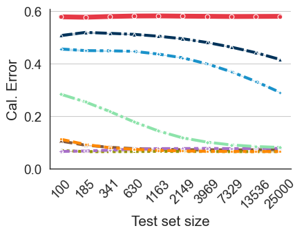
(a) ResNet 152 on ImageNet

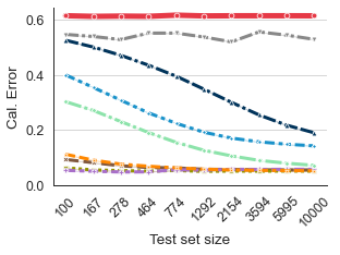
(b) LeNet 5 on CIFAR10

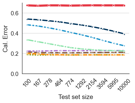
(c) ResNet 110 on CIFAR100

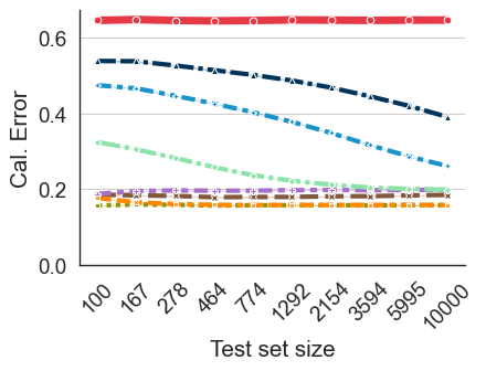
(d) ResNet 110 SD on CIFAR100

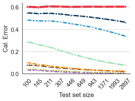
(e) ResNet 50 on BIRDS

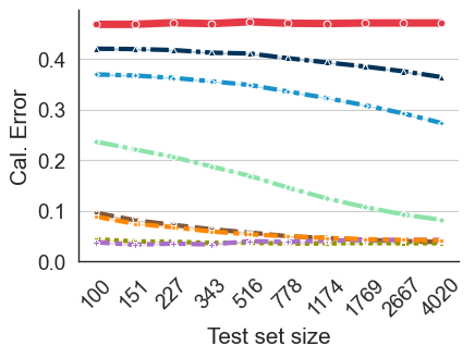
(f) ResNet 101 on CARS

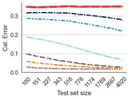
(g) Pretrained ResNet 101 on CARS

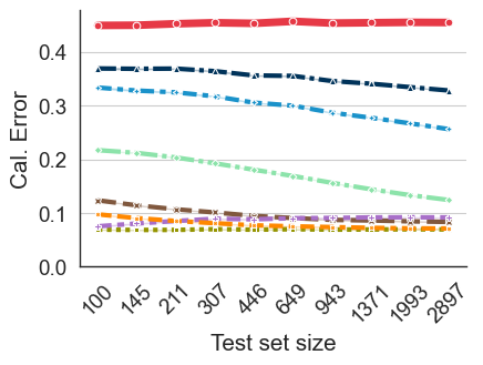
(h) ResNet 50 NTS on BIRDS

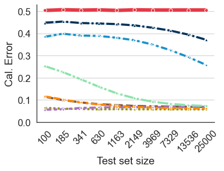
(i) PNASNet5 Large on ImageNet

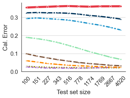
(j) Pretrained ResNet 50 on CARS

(k) ResNet 110 SD on CIFAR100

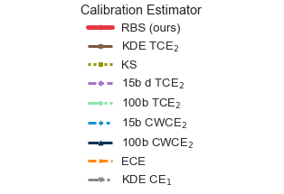
Figure 5: Different calibration error estimates versus the test set size. The red line corresponds to the square root of the Brier score which is an upper bound of $\text{CE}_{2}$. The other estimators are lower bounds.

G.4 Recalibration improvement

In the main text we investigated recalibration improvement of common estimators for the calibration error and compared their reliability to RBS. According to Proposition 4.5 and since RBS is asymptotically unbiased and consistent, it can be regarded as a reliable approximation of the real improvement of the recalibration methods. However, if we move to the squared space, our proposed upper bound is even provably reliable since it has a minimum-variance unbiased estimator. This motivates further experiments comparing existing calibration errors in the squared space, which we describe in the following. Here, we first report additional results comparing common estimators to RBS; we then report results in the squared space. We start with a formal description of the problem and experimental setup.

Let $D$ be a sampled subset of the full test set. Let $f$ be the underlying model and $h$ an optimized recalibration method. Let $e$ be an calibration error estimator taking a dataset and a model as inputs. The recalibration improvement according to estimator $e$ is estimated via $e\left(D,f\right)-e\left(D,h\circ f\right)$.

Recalibration improvement of common estimators

We compute the recalibration improvement of common estimators on several test set samples of a given size and plot the average of these on the y-axis. We extend the results reported in the main text by covering additional datasets, models and architectures. These extended experiments confirm the findings reported in the main text, namely that only RBS reliably quantifies the improvement in calibration error after recalibration (Fig. 6; standard errors are shown).

Recalibration improvement in the squared space

The recalibration improvement in the squared space according to estimator $e$ is estimated via $\left(e\left(D,f\right)\right)^{2}-\left(e\left(D,h\circ f\right)\right)^{2}$. The results are depicted in Figure 7. For CIFAR10, we also included the KDE estimator for CE${}_{2}^{2}$ according to [43]. Only the Brier score (square of RBS) yields provably unbiased estimates of the true recalibration improvement w.r.t. CE${}_{2}^{2}$. In contrast to our approach, all other estimators are sensitive to test set size and/or substantially underestimate the true recalibration improvement in squared space.

For larger subsets of the CIFAR100 test set, the automatic bandwidth optimization for KDE CE₂ does not return a valid bandwidth. These cases are omitted from Figure 7(b) and 7(e). We also omitted KDE CE₁ as it shows similar behaviour as KDE CE₂ but is shifted substantially towards the negative like in the CIFAR10 case (Fig. 7(d)).

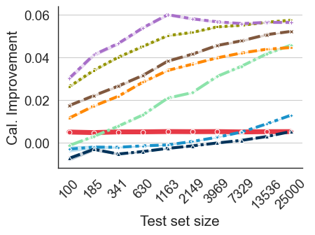
(a) TS applied to ResNet 152
on ImageNet

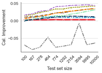
(b) TS applied to LeNet 5
on CIFAR10

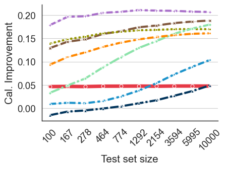
(c) TS applied to ResNet 110
on CIFAR100

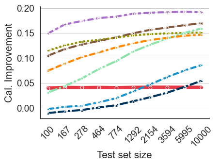
(d) TS applied to ResNet 110 SD
on CIFAR100

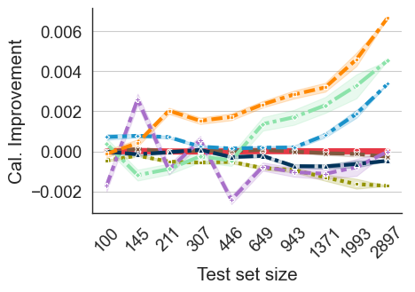
(e) TS applied to ResNet 50
on BIRDS

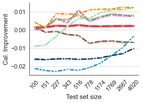
(f) DIAG applied to ResNet 101
on CARS

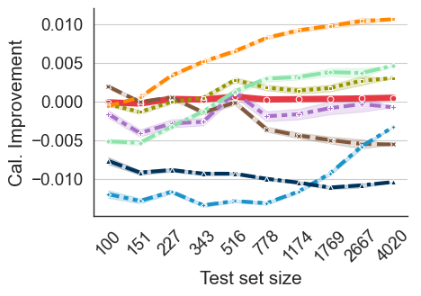
(g) DIAG applied to
pretrained ResNet 101 on CARS

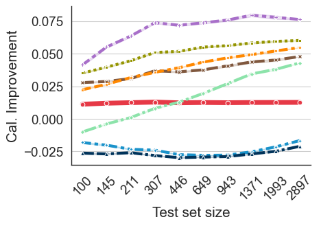
(h) DIAG applied to
ResNet 50 NTS on BIRDS

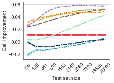
(i) DIAG applied to PNASNet5 Large
on ImageNet

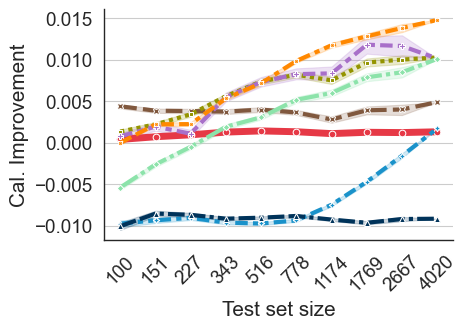
(j) DIAG applied to
pretrained ResNet 50 on CARS

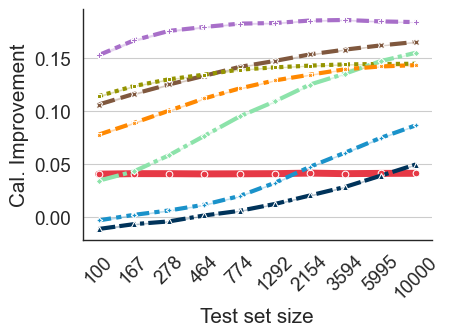
(k) ETS applied to ResNet 110 SD
on CIFAR100

Figure 6: Different calibration improvement estimates versus the test set size. The red line corresponds to the square root of the Brier score.

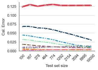
(a) DenseNet 40 on CIFAR10

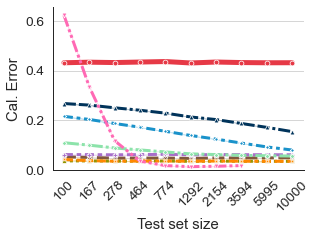
(b) Wide ResNet 32 on CIFAR100

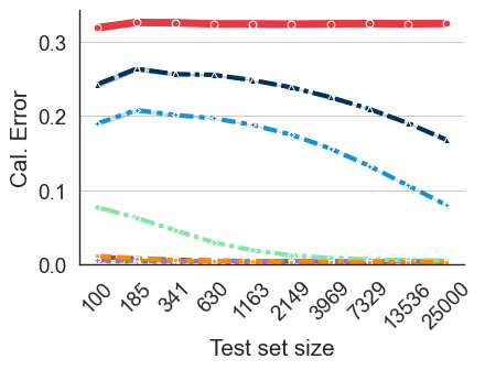
(c) DenseNet 161 on ImageNet

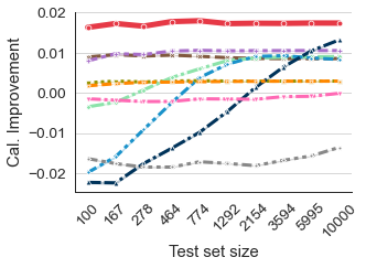
(d) DenseNet 40 on CIFAR10

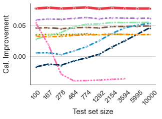
(e) Wide ResNet 32 on CIFAR100

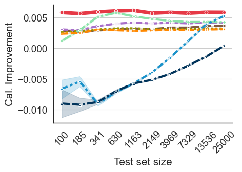
(f) DenseNet 161 on ImageNet

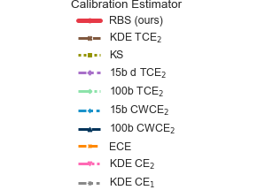
Figure 7: First row: Different squared calibration error estimates versus the test set size. The red line corresponds to the Brier score which is an upper bound of $\text{CE}_{2}^{2}$. The other errors are lower bounds. Second row: Estimated improvements in the squared space of injective recalibration methods in different settings. Our approach captures the true improvement w.r.t. $\text{CE}_{2}^{2}$ in an unbiased manner.

G.5 Variance regression

In the following, we give more details on the variance regression experiment in the main paper, but also add further results of the Friedman 1 regression problem.

In all following scenarios, we are interested in the effect of recalibration towards predictive uncertainty. For this, we use Platt scaling ($x\to wx+b$ with parameters $w,b\in\mathbb{R}$) of the variance output and optimize $w$ and $b$ with the L-BFGS optimizer on the validation set. Further, since Platt scaling is injective, we apply Theorem 4.3 and Proposition 4.5 to treat the DSS score as an calibration error for recalibration. Consequently, optimizing Platt scaling with the DSS score is equivalent to optimizing the associated calibration error.

We will use this recalibration procedure in each iteration during model training, but without modifying the model for the next training step.

Widmann et al. [58] used the MSE as training objective, while we use the DSS, as it is a natural extension of the MSE to variance regression.

We repeat each experiment with five distinct seeds and aggregate the results, giving the characteristic error bands in each figure.

G.5.1 UCI dataset Residential Building

The Residential Building dataset consists of 107 features and 372 data instances. To have similar conditions as the Friedman 1 regression problem in the next section, we split the dataset into a training, validation, and test set with sizes 100, 100, and 173. We use a fully-connected mixture density network as Widmann et al. [58], except we are also using an output node for the variance prediction, and reduce its size for a more stable training. Specifically, it consists of 107 input nodes, 200 hidden nodes, and 2 output nodes. Similar to Widmann et al. [58], we use Adam as model optimizer with default parameters ($0.001$ learning rate, $0.9$ first momentum decay, $0.999$ second momentum decay).

We show similar results as in Figure 4 but with aggregations from different runs with distinct seeds. The evaluations are depicted in 8 and repeat the findings in the main paper.

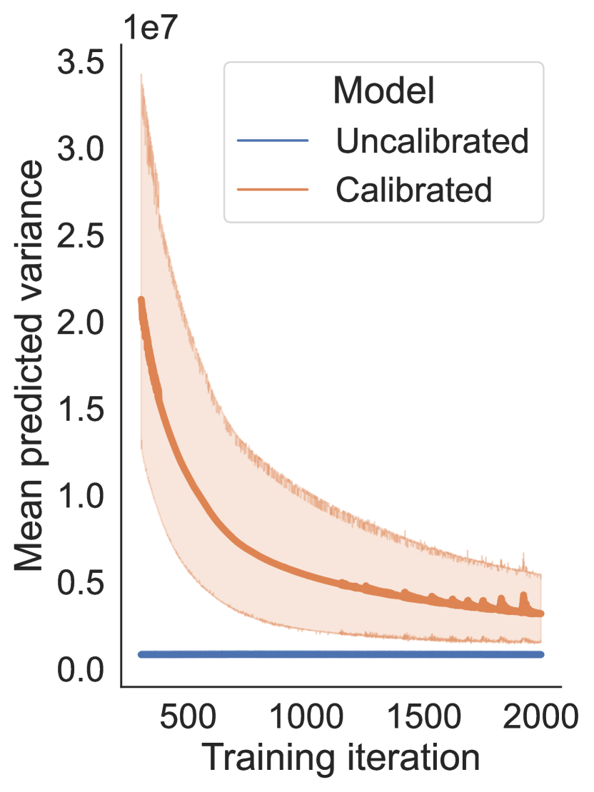
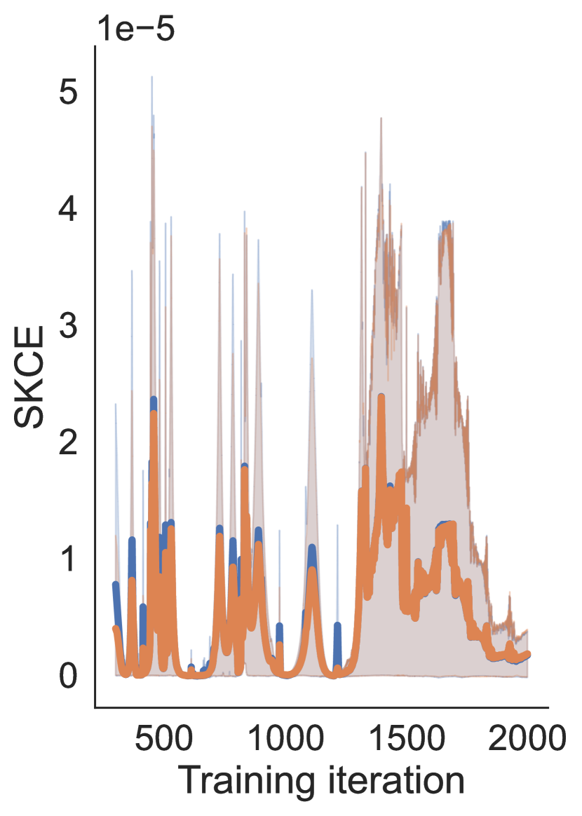
Figure 8: Left: Average predicted variance throughout model training before and after recalibration. Initially, due to a bad fit, recalibration adjusts the variance accordingly for better communicated uncertainty. Once the model fit improves, the predicted variance requires less adjustment due to less uncertainty in each prediction. Middle: DSS communicates reasonably changes in the variance due to recalibration. Right: SKCE fails to capture the variance trend and behaves erratically.

G.5.2 Friedman 1

The Friedman 1 regression problem consists of ten feature variables but only five influence the target variable [11]. The target variable is given by

$$Y=10\sin(\pi X_{1}X_{2})+20(X_{3}-0.5)^{2}+10X_{4}+5X_{5}+\epsilon$$ (56)

with input $X_{i}\sim U\left(0,1\right)$ independently uniformly distributed for $i=1,\dots,10$, and noise $\epsilon\sim\mathscr{N}\left(0,1\right)$. It was used lately to investigate model calibration in the regression case [58]. We slightly modify the Friedman 1 regression problem to have varying variance depending on the sixth feature variable, i.e. $\epsilon\sim\mathscr{N}\left(0,0.5+X_{6}\right)$. This makes it non-trivial to give an estimate of the predictive uncertainty in the form of the predicted variance. We sample a training, validation, and test set, each of size 100 similar to Widmann et al. [58].

We use the same fully-connected mixture density network as Widmann et al. [58], except we are also using an output node for the variance prediction. Further, we use the same training details as Widmann et al. [58]. We repeat each run three times and aggregate the results.

We again compare DSS, SKCE, and average predicted variance throughout model training with and without recalibration. We depict the performance according to various errors during model training in Figure 9. As can be seen, recalibration adjusts overfitting of the predicted variance. Consequently, the uncertainty communication of the model is improved. Further, the SKCE seems to be less influenced by the variance calibration and more so by the mean calibration. This is a significant drawback when uncertainty communication is done via the predicted variance.

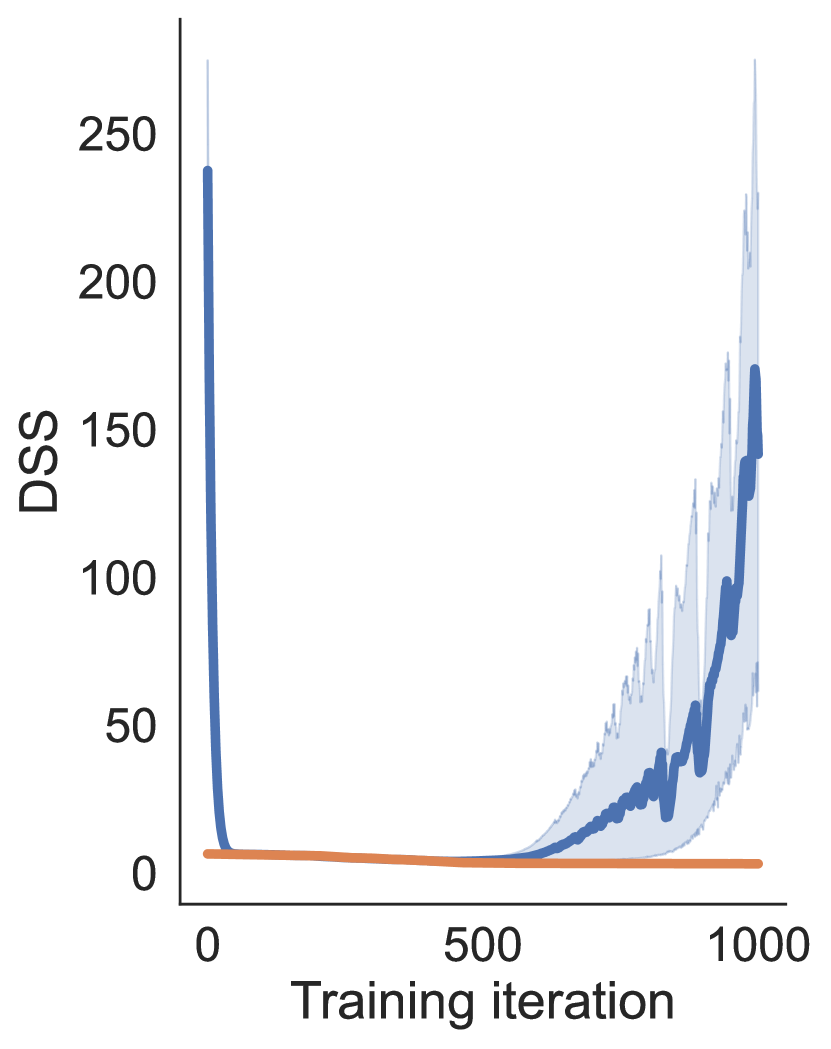
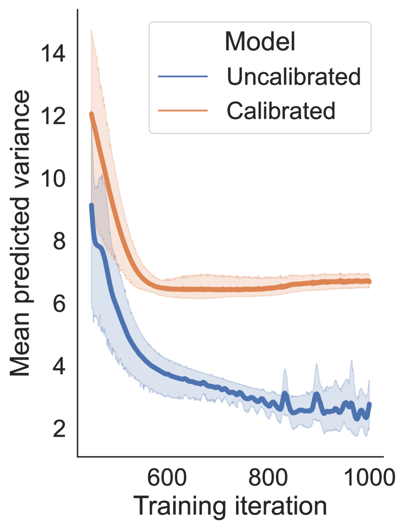
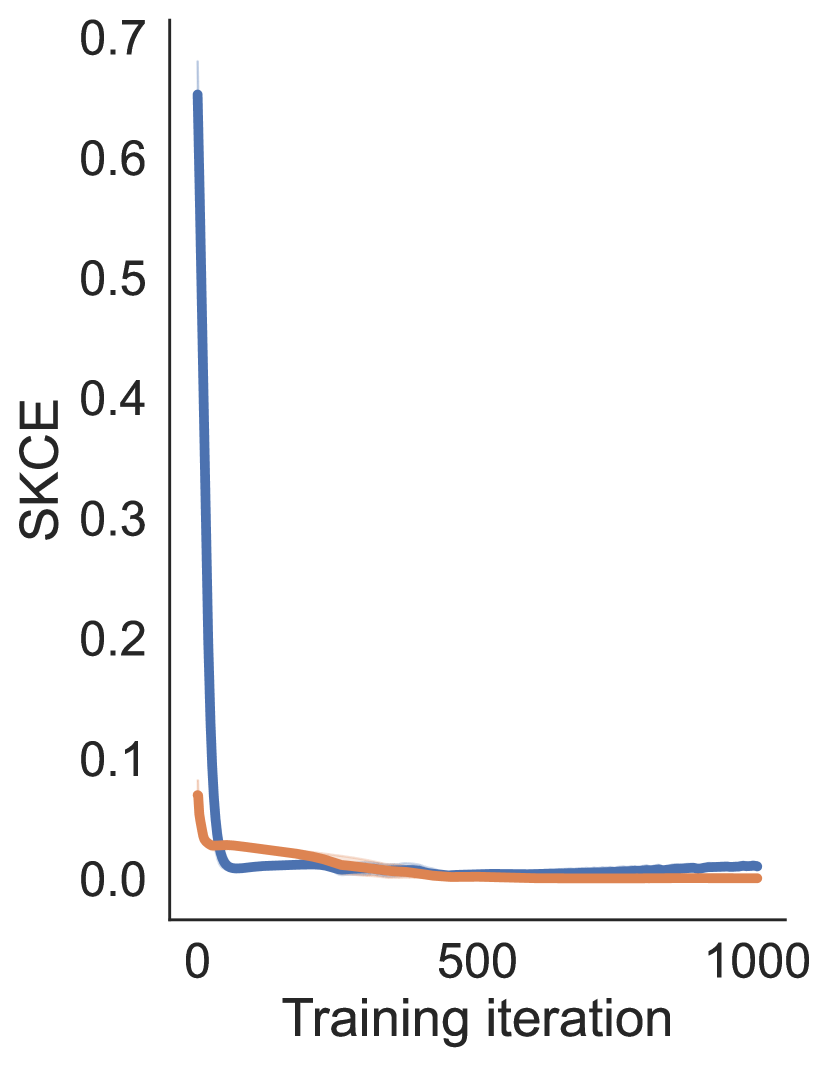
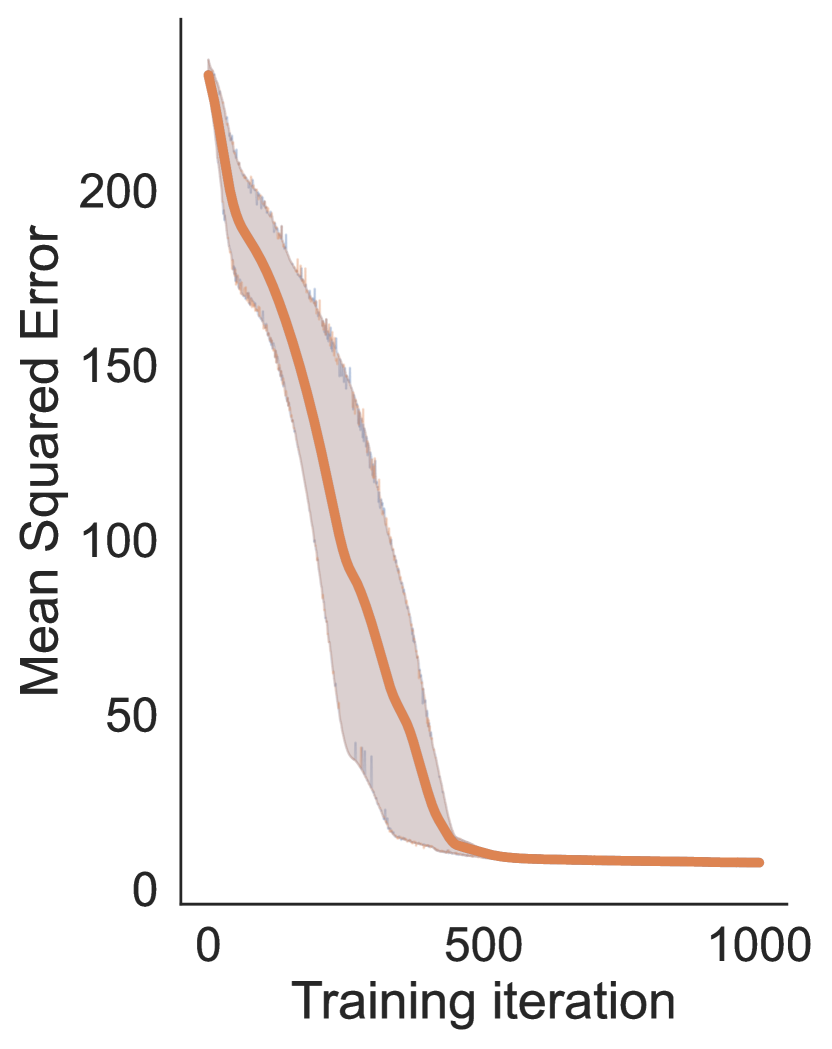
Figure 9: Upper left: DSS shows that overfitting occurs at some point during training. Recalibration successfully adjusts this overfit. This indicates that most of the overfit is regarding variance and not mean prediction. Upper right: Average predicted variance starting from the point of overfitting. Recalibration adjusts the steadily decreasing predicted variance to a constant level. Lower left: SKCE signals improved calibration at the start of training but remains relatively unchanged by the variance overfit. Lower right: The MSE curve confirms that the predicted mean is not overfitted and suggests the SKCE is more sensitive to the calibration of the mean than the calibration of the variance estimate. Our recalibration does not influence the predicted mean, thus we omit the recalibrated model from this subfigure.

References

• Aitchison & Shen [1980] Aitchison, J. and Shen, S. M. Logistic-normal distributions: Some properties and uses. Biometrika, 67(2):261–272, 1980. ISSN 00063444. URL http://www.jstor.org/stable/2335470.
• Bishop [1994] Bishop, C. M. Mixture density networks. 1994.
• Brier [1950] Brier, G. W. Verification of forecasts expressed in terms of probability. Monthly Weather Review, 78(1):1 – 3, 1950. doi: 10.1175/1520-0493(1950)078<0001:VOFEIT>2.0.CO;2. URL https://journals.ametsoc.org/view/journals/mwre/78/1/1520-0493_1950_078_0001_vofeit_2_0_co_2.xml.
• Bröcker [2009] Bröcker, J. Reliability, sufficiency, and the decomposition of proper scores. Quarterly Journal of the Royal Meteorological Society, 135(643):1512–1519, Jul 2009. ISSN 1477-870X. doi: 10.1002/qj.456. URL http://dx.doi.org/10.1002/qj.456.
• Capiński & Kopp [2004] Capiński, M. and Kopp, P. E. Measure, integral and probability, volume 14. Springer, 2004.
• Chung et al. [2021] Chung, Y., Neiswanger, W., Char, I., and Schneider, J. Beyond pinball loss: Quantile methods for calibrated uncertainty quantification, 2021.
• Dawid [1982] Dawid, A. P. The well-calibrated bayesian. Journal of the American Statistical Association, 77(379):605–610, 1982. doi: 10.1080/01621459.1982.10477856. URL https://www.tandfonline.com/doi/abs/10.1080/01621459.1982.10477856.
• Dawid & Sebastiani [1999] Dawid, A. P. and Sebastiani, P. Coherent dispersion criteria for optimal experimental design. Annals of Statistics, pp.  65–81, 1999.
• Deng et al. [2009] Deng, J., Dong, W., Socher, R., Li, L.-J., Li, K., and Fei-Fei, L. Imagenet: A large-scale hierarchical image database. In 2009 IEEE conference on computer vision and pattern recognition, pp.  248–255. Ieee, 2009.
• Fan et al. [2022] Fan, H., Ferianc, M., Que, Z., Niu, X., Rodrigues, M. L., and Luk, W. Accelerating bayesian neural networks via algorithmic and hardware optimizations. IEEE Transactions on Parallel and Distributed Systems, 2022.
• Friedman [1991] Friedman, J. H. Multivariate adaptive regression splines. The annals of statistics, 19(1):1–67, 1991.
• Gneiting & Katzfuss [2014] Gneiting, T. and Katzfuss, M. Probabilistic forecasting. Annual Review of Statistics and Its Application, 1:125–151, 2014.
• Gneiting & Raftery [2007] Gneiting, T. and Raftery, A. E. Strictly proper scoring rules, prediction, and estimation. Journal of the American Statistical Association, 102(477):359–378, 2007. doi: 10.1198/016214506000001437. URL https://doi.org/10.1198/016214506000001437.
• Guo et al. [2017] Guo, C., Pleiss, G., Sun, Y., and Weinberger, K. Q. On calibration of modern neural networks. In International Conference on Machine Learning, pp. 1321–1330. PMLR, 2017.
• Gupta et al. [2021] Gupta, A., Kvernadze, G., and Srikumar, V. Bert & family eat word salad: Experiments with text understanding. ArXiv, abs/2101.03453, 2021.
• Gupta et al. [2020] Gupta, K., Rahimi, A., Ajanthan, T., Mensink, T., Sminchisescu, C., and Hartley, R. Calibration of neural networks using splines. In International Conference on Learning Representations, 2020.
• Haggenmüller et al. [2021] Haggenmüller, S., Maron, R. C., Hekler, A., Utikal, J. S., Barata, C., Barnhill, R. L., Beltraminelli, H., Berking, C., Betz-Stablein, B., Blum, A., Braun, S. A., Carr, R., Combalia, M., Fernandez-Figueras, M.-T., Ferrara, G., Fraitag, S., French, L. E., Gellrich, F. F., Ghoreschi, K., Goebeler, M., Guitera, P., Haenssle, H. A., Haferkamp, S., Heinzerling, L., Heppt, M. V., Hilke, F. J., Hobelsberger, S., Krahl, D., Kutzner, H., Lallas, A., Liopyris, K., Llamas-Velasco, M., Malvehy, J., Meier, F., Müller, C. S., Navarini, A. A., Navarrete-Dechent, C., Perasole, A., Poch, G., Podlipnik, S., Requena, L., Rotemberg, V. M., Saggini, A., Sangueza, O. P., Santonja, C., Schadendorf, D., Schilling, B., Schlaak, M., Schlager, J. G., Sergon, M., Sondermann, W., Soyer, H. P., Starz, H., Stolz, W., Vale, E., Weyers, W., Zink, A., Krieghoff-Henning, E., Kather, J. N., von Kalle, C., Lipka, D. B., Fröhling, S., Hauschild, A., Kittler, H., and Brinker, T. J. Skin cancer classification via convolutional neural networks: systematic review of studies involving human experts. European Journal of Cancer, 156:202–216, 2021. ISSN 0959-8049. doi: https://doi.org/10.1016/j.ejca.2021.06.049. URL https://www.sciencedirect.com/science/article/pii/S0959804921004445.
• Hastie & Tibshirani [1998] Hastie, T. and Tibshirani, R. Classification by pairwise coupling. The annals of statistics, 26(2):451–471, 1998.
• He et al. [2015] He, K., Zhang, X., Ren, S., and Sun, J. Delving deep into rectifiers: Surpassing human-level performance on imagenet classification. In Proceedings of the IEEE international conference on computer vision, pp.  1026–1034, 2015.
• He et al. [2016] He, K., Zhang, X., Ren, S., and Sun, J. Deep residual learning for image recognition. In Proceedings of the IEEE conference on computer vision and pattern recognition, pp.  770–778, 2016.
• Hoeffding [1948] Hoeffding, W. A Class of Statistics with Asymptotically Normal Distribution. The Annals of Mathematical Statistics, 19(3):293 – 325, 1948. doi: 10.1214/aoms/1177730196. URL https://doi.org/10.1214/aoms/1177730196.
• Huang et al. [2017] Huang, G., Liu, Z., Van Der Maaten, L., and Weinberger, K. Q. Densely connected convolutional networks. In Proceedings of the IEEE conference on computer vision and pattern recognition, pp.  4700–4708, 2017.
• Islam et al. [2021] Islam, A., Chen, C.-F., Panda, R., Karlinsky, L., Radke, R. J., and Feris, R. S. A broad study on the transferability of visual representations with contrastive learning. 2021 IEEE/CVF International Conference on Computer Vision (ICCV), pp.  8825–8835, 2021.
• Joo et al. [2020] Joo, T., Chung, U., and Seo, M. Being bayesian about categorical probability. In ICML, 2020.
• Katsaouni et al. [2021] Katsaouni, N., Tashkandi, A., Wiese, L., and Schulz, M. H. Machine learning based disease prediction from genotype data. Biological Chemistry, 402(8):871–885, 2021. doi: doi:10.1515/hsz-2021-0109. URL https://doi.org/10.1515/hsz-2021-0109.
• Kristiadi et al. [2020] Kristiadi, A., Hein, M., and Hennig, P. Being bayesian, even just a bit, fixes overconfidence in relu networks. In ICML, 2020.
• Krizhevsky et al. [2009] Krizhevsky, A. et al. Learning multiple layers of features from tiny images. 2009.
• Kull et al. [2017] Kull, M., Filho, T. S., and Flach, P. Beta calibration: a well-founded and easily implemented improvement on logistic calibration for binary classifiers. In Singh, A. and Zhu, J. (eds.), Proceedings of the 20th International Conference on Artificial Intelligence and Statistics, volume 54 of Proceedings of Machine Learning Research, pp.  623–631. PMLR, 20–22 Apr 2017. URL https://proceedings.mlr.press/v54/kull17a.html.
• Kull et al. [2019] Kull, M., Perello Nieto, M., Kängsepp, M., Silva Filho, T., Song, H., and Flach, P. Beyond temperature scaling: Obtaining well-calibrated multi-class probabilities with dirichlet calibration. Advances in Neural Information Processing Systems, 32:12316–12326, 2019.
• Kumar et al. [2018] Kumar, A., Sarawagi, S., and Jain, U. Trainable calibration measures for neural networks from kernel mean embeddings. In Dy, J. and Krause, A. (eds.), Proceedings of the 35th International Conference on Machine Learning, volume 80 of Proceedings of Machine Learning Research, pp.  2805–2814. PMLR, 10–15 Jul 2018. URL https://proceedings.mlr.press/v80/kumar18a.html.
• Kumar et al. [2019] Kumar, A., Liang, P., and Ma, T. Verified uncertainty calibration. In Proceedings of the 33rd International Conference on Neural Information Processing Systems, pp.  3792–3803, 2019.
• LeCun et al. [1998] LeCun, Y., Bottou, L., Bengio, Y., and Haffner, P. Gradient-based learning applied to document recognition. Proceedings of the IEEE, 86(11):2278–2324, 1998.
• Liu et al. [2018] Liu, C., Zoph, B., Neumann, M., Shlens, J., Hua, W., Li, L.-J., Fei-Fei, L., Yuille, A., Huang, J., and Murphy, K. Progressive neural architecture search. In Proceedings of the European conference on computer vision (ECCV), pp.  19–34, 2018.
• Maddox et al. [2019] Maddox, W. J., Izmailov, P., Garipov, T., Vetrov, D. P., and Wilson, A. G. A simple baseline for bayesian uncertainty in deep learning. Advances in Neural Information Processing Systems, 32:13153–13164, 2019.
• Menon et al. [2021] Menon, A. K., Rawat, A. S., Reddi, S. J., Kim, S., and Kumar, S. A statistical perspective on distillation. In ICML, 2021.
• Minderer et al. [2021] Minderer, M., Djolonga, J., Romijnders, R., Hubis, F., Zhai, X., Houlsby, N., Tran, D., and Lucic, M. Revisiting the calibration of modern neural networks. Advances in Neural Information Processing Systems, 34, 2021.
• Morales-Álvarez et al. [2021] Morales-Álvarez, P., Hernández-Lobato, D., Molina, R., and Hernández-Lobato, J. M. Activation-level uncertainty in deep neural networks. In ICLR, 2021.
• Murphy [1973] Murphy, A. H. A new vector partition of the probability score. Journal of Applied Meteorology and Climatology, 12(4):595 – 600, 1973. doi: 10.1175/1520-0450(1973)012<0595:ANVPOT>2.0.CO;2. URL https://journals.ametsoc.org/view/journals/apme/12/4/1520-0450_1973_012_0595_anvpot_2_0_co_2.xml.
• Naeini et al. [2015] Naeini, M. P., Cooper, G. F., and Hauskrecht, M. Obtaining well calibrated probabilities using bayesian binning. In Proceedings of the Twenty-Ninth AAAI Conference on Artificial Intelligence, AAAI’15, pp.  2901–2907. AAAI Press, 2015. ISBN 0262511290.
• Nguyen & O’Connor [2015] Nguyen, K. and O’Connor, B. Posterior calibration and exploratory analysis for natural language processing models. In Proceedings of the 2015 Conference on Empirical Methods in Natural Language Processing, pp.  1587–1598, 2015.
• Nixon et al. [2019] Nixon, J., Dusenberry, M. W., Zhang, L., Jerfel, G., and Tran, D. Measuring calibration in deep learning. In CVPR Workshops, volume 2, 2019.
• Platt [1999] Platt, J. C. Probabilistic outputs for support vector machines and comparisons to regularized likelihood methods. In Advances in Large-Margin Classifiers, pp.  61–74. MIT Press, 1999.
• Popordanoska et al. [2022] Popordanoska, T., Sayer, R., and Blaschko, M. B. A consistent and differentiable lp canonical calibration error estimator. In Oh, A. H., Agarwal, A., Belgrave, D., and Cho, K. (eds.), Advances in Neural Information Processing Systems, 2022. URL https://openreview.net/forum?id=HMs5pxZq1If.
• Rafiei & Adeli [2016] Rafiei, M. H. and Adeli, H. A novel machine learning model for estimation of sale prices of real estate units. Journal of Construction Engineering and Management, 142(2):04015066, 2016.
• Rahimi et al. [2020] Rahimi, A., Shaban, A., Cheng, C.-A., Hartley, R., and Boots, B. Intra order-preserving functions for calibration of multi-class neural networks. Advances in Neural Information Processing Systems, 33:13456–13467, 2020.
• Roelofs et al. [2021] Roelofs, R., Cain, N., Shlens, J., and Mozer, M. C. Mitigating bias in calibration error estimation, 2021.
• Schrittwieser et al. [2020] Schrittwieser, J., Antonoglou, I., Hubert, T., Simonyan, K., Sifre, L., Schmitt, S., Guez, A., Lockhart, E., Hassabis, D., Graepel, T., et al. Mastering atari, go, chess and shogi by planning with a learned model. Nature, 588(7839):604–609, 2020.
• Song et al. [2019] Song, H., Diethe, T., Kull, M., and Flach, P. Distribution calibration for regression. In International Conference on Machine Learning, pp. 5897–5906. PMLR, 2019.
• Takeshi [1985] Takeshi, A. Advanced econometrics. Harvard university press, 1985.
• Tian et al. [2021] Tian, J., Yung, D., Hsu, Y.-C., and Kira, Z. A geometric perspective towards neural calibration via sensitivity decomposition. In NeurIPS, 2021.
• Tomani et al. [2021] Tomani, C., Gruber, S., Erdem, M. E., Cremers, D., and Buettner, F. Post-hoc uncertainty calibration for domain drift scenarios. In Proceedings of the IEEE/CVF Conference on Computer Vision and Pattern Recognition (CVPR), pp.  10124–10132, June 2021.
• Tsagris et al. [2014] Tsagris, M., Beneki, C., and Hassani, H. On the folded normal distribution. Mathematics, 2(1):12–28, feb 2014. doi: 10.3390/math2010012. URL https://doi.org/10.3390%2Fmath2010012.
• Vaicenavicius et al. [2019] Vaicenavicius, J., Widmann, D., Andersson, C., Lindsten, F., Roll, J., and Schön, T. Evaluating model calibration in classification. In The 22nd International Conference on Artificial Intelligence and Statistics, pp.  3459–3467. PMLR, 2019.
• Wang et al. [2021] Wang, X., Liu, H., Shi, C., and Yang, C. Be confident! towards trustworthy graph neural networks via confidence calibration. In NeurIPS, 2021.
• Wehenkel & Louppe [2019] Wehenkel, A. and Louppe, G. Unconstrained monotonic neural networks. Advances in Neural Information Processing Systems, 32:1545–1555, 2019.
• Wenger et al. [2020] Wenger, J., Kjellström, H., and Triebel, R. Non-parametric calibration for classification. In International Conference on Artificial Intelligence and Statistics, pp.  178–190. PMLR, 2020.
• Widmann et al. [2019] Widmann, D., Lindsten, F., and Zachariah, D. Calibration tests in multi-class classification: A unifying framework. Advances in Neural Information Processing Systems, 32:12257–12267, 2019.
• Widmann et al. [2021] Widmann, D., Lindsten, F., and Zachariah, D. Calibration tests beyond classification. In International Conference on Learning Representations, 2021. URL https://openreview.net/forum?id=-bxf89v3Nx.
• Yen et al. [2019] Yen, M.-H., Liu, D.-W., Hsin, Y.-C., Lin, C.-E., and Chen, C.-C. Application of the deep learning for the prediction of rainfall in southern taiwan. Scientific reports, 9(1):1–9, 2019.
• Zadrozny & Elkan [2001] Zadrozny, B. and Elkan, C. Obtaining calibrated probability estimates from decision trees and naive bayesian classifiers. ICML, 1, 05 2001.
• Zadrozny & Elkan [2002] Zadrozny, B. and Elkan, C. Transforming classifier scores into accurate multiclass probability estimates. In Proceedings of the Eighth ACM SIGKDD International Conference on Knowledge Discovery and Data Mining, KDD ’02, pp.  694–699, New York, NY, USA, 2002. Association for Computing Machinery. ISBN 158113567X. doi: 10.1145/775047.775151. URL https://doi.org/10.1145/775047.775151.
• Zagoruyko & Komodakis [2016] Zagoruyko, S. and Komodakis, N. Wide residual networks. In British Machine Vision Conference 2016. British Machine Vision Association, 2016.
• Zhang et al. [2020] Zhang, J., Kailkhura, B., and Han, T. Y.-J. Mix-n-match: Ensemble and compositional methods for uncertainty calibration in deep learning. In International Conference on Machine Learning, pp. 11117–11128. PMLR, 2020.