Optimal denoising of rotationally invariant rectangular matrices

Abstract

In this manuscript we consider denoising of large rectangular matrices: given a noisy observation of a signal matrix, what is the best way of recovering the signal matrix itself? For Gaussian noise and rotationally-invariant signal priors, we completely characterize the optimal denoiser and its performance in the high-dimensional limit, in which the size of the signal matrix goes to infinity with fixed aspects ratio, and under the Bayes optimal setting, that is when the statistician knows how the signal and the observations were generated. Our results generalise previous works that considered only symmetric matrices to the more general case of non-symmetric and rectangular ones. We explore analytically and numerically a particular choice of factorized signal prior that models cross-covariance matrices and the matrix factorization problem. As a byproduct of our analysis, we provide an explicit asymptotic evaluation of the rectangular Harish-Chandra-Itzykson-Zuber integral in a special case.

1 Introduction

In this paper we consider the problem of denoising large rectangular matrices, i.e. the problem of reconstructing a matrix ${\boldsymbol{S}}^{*}\in\mathbb{R}^{m\times p}$ from a noisy observation ${\boldsymbol{Y}}=P_{\rm noise}({\boldsymbol{S}}^{*})\in\mathbb{R}^{m\times p}$. Our aim is to characterize theoretically this problem in the Bayes optimal setting, in which the statistician knows the details of the prior distribution of the signal $P_{\rm signal}$ and the noisy channel $P_{\rm noise}$. In particular, we will consider the case of additive Gaussian noise $P_{\rm noise}({\boldsymbol{S}}^{*})={\boldsymbol{S}}^{*}+\sqrt{\Delta}{\boldsymbol{Z}}$ where $\Delta>0$ controls the strength of the noise, and ${\boldsymbol{Z}}\in\mathbb{R}^{m\times p}$ is a matrix of i.i.d. Gaussian random variables. On the side of the signal we will consider rotationally invariant priors, i.e. those where $P_{\rm signal}({\boldsymbol{S}}^{*})=P_{\rm signal}({\boldsymbol{U}}{\boldsymbol{S}}^{*}{\boldsymbol{V}})$ for any pair of rotation matrices ${\boldsymbol{U}}\in\mathcal{O}({m}),{\boldsymbol{V}}\in\mathcal{O}({p})$.

We are interested in particular in the case of factorized priors, i.e. ${\boldsymbol{S}}^{*}={\boldsymbol{F}}{\boldsymbol{X}}$ with ${\boldsymbol{F}}\in\mathbb{R}^{m\times r}$ and ${\boldsymbol{X}}\in\mathbb{R}^{r\times p}$, and both ${\boldsymbol{X}}$ and ${\boldsymbol{F}}$ having i.i.d. Gaussian entries. From the point of view of applications, this is equivalent to the problem of denoising cross-correlation matrices, which is, for example, extremely relevant in modern financial portfolio theory where it allows to compute better performing investment portfolios by reducing overfitting Bun et al. [2017].

From a theoretical point of view, the denoising problem is a simpler variant of the matrix factorization problem, where one would like to reconstruct the two factors ${\boldsymbol{F}}$ and ${\boldsymbol{X}}$ from the noisy observation ${\boldsymbol{Y}}$. Matrix factorization is ubiquitous in computer science, modeling many applications, from sparse PCA Johnstone and Lu [2009] to dictionary learning Mairal et al. [2009]. While well studied in the low-rank regime $r=\Theta(1)$ and $\min(p,m)\to\infty$, where optimal estimators and guarantees on their performances are available Lesieur et al. [2017], Miolane [2018], much less is known in the extensive-rank regime, where $r$ is of the same order as $m$ and $p$.

This setting was studied, for generic priors on elements of ${\boldsymbol{F}}$ and ${\boldsymbol{X}}$, in Kabashima et al. [2016], where an analysis of the information-theoretic thresholds and the performance of approximate message passing algorithms was given. A more recent series of works pointed out however that a key assumption of Kabashima et al. [2016] does not hold in practice, and proposed alternative analysis techniques, ranging from spectral characterizations Schmidt [2018], Barbier and Macris [2021] to high-temperature expansions Maillard et al. [2021]. In all these cases, the analytical results obtained for rectangular matrices are not explicit and of limited practical applicability even in the very simple case of Gaussian priors on the factors and additive Gaussian noise. Studying the denoising problem in the Gaussian regime is thus a first step towards a better understanding of matrix factorization in this challenging regime.

Our main results concern rotationally invariant priors, i.e. signal matrices whose information lies exclusively in the distribution of their singular values, corrupted by additive Gaussian noise. For this large class of priors, we compute the optimal denoiser (in the sense of the mean square error on the matrix ${\boldsymbol{S}}$) and its performance in the Bayes optimal setting, and we discuss in detail the case of factorized priors where both the factors ${\boldsymbol{F}}$ and ${\boldsymbol{X}}$ have i.i.d. Gaussian components. As a byproduct of our analysis, we also provide an explicit formula for the high-dimensional asymptotics of the rectangular HCIZ integral Harish-Chandra [1957], Itzykson and Zuber [1980], Guionnet and Huang [2021] in a special case.

The code for the numerical simulations and for reproducing the figures is available here: https://github.com/PenombraET/rectangular_RIE

1.1 Definition of the model

In this paper we focus our attention to rotationally-invariant priors, i.e. $P_{\rm signal}({\boldsymbol{S}})=P_{\rm signal}({\boldsymbol{U}}{\boldsymbol{S}}{\boldsymbol{V}})$ for any pair of rotation matrices ${\boldsymbol{U}}\in\mathcal{O}({m}),{\boldsymbol{V}}\in\mathcal{O}({p})$, where $\mathcal{O}({m})$ is the orthogonal group in $m$ dimensions, and additive white Gaussian noise ${\boldsymbol{Z}}$ being a matrix of i.i.d. Gaussian random variables with zero mean and variance $(mp)^{-1/2}$. The rotational invariance of the prior, together with the rotational invariance of Gaussian noise, implies that the observation ${\boldsymbol{Y}}$ will have a rotationally-invariant distribution, and that all relevant observables of the problem will depend only on the singular value distributions of ${\boldsymbol{S}},{\boldsymbol{Z}}$ and ${\boldsymbol{Y}}$.

In order for the signal-to-noise ratio (SNR) $\sqrt{\Delta}$ to be comparable over different choices of priors, we fix the ratio between the averaged $L^{2}$ norm of the signal matrix ${\boldsymbol{S}}$ and that of the noise matrix ${\boldsymbol{Z}}$ to 1. Explicitly, one requires that

$$\mathbb{E}_{\rm prior}[||{\boldsymbol{S}}||_{2}^{2}]=\mathbb{E}_{\rm noise}[||{\boldsymbol{Z}}||_{2}^{2}]=\sqrt{mp}\,,$$ (1)

where the $L^{2}$ norm is defined as $||{\boldsymbol{S}}||_{2}^{2}=\operatorname{Tr}({\boldsymbol{S}}{\boldsymbol{S}}^{T})$. We will consider the high-dimensional regime, i.e. the limit $m,p\to\infty$ with fixed ratio $R_{1}\equiv p/m.$ Without loss of generality, we will consider $p\geq m$, i.e. $R_{1}\geq 1$. We require that in this limit the singular values of the signal are of order $\mathcal{O}(1)$, and that the corresponding empirical singular value density of the prior converges to a deterministic probability density function.

As a particular choice of rotationally-invariant prior, we focus on on factorized signals, i.e.

$${\boldsymbol{S}}^{*}=\frac{{\boldsymbol{F}}{\boldsymbol{X}}}{\sqrt{r}\sqrt[4]{mp}}\,,$$ (2)

where ${\boldsymbol{F}}\in\mathbb{R}^{m\times r}$, ${\boldsymbol{X}}\in\mathbb{R}^{r\times p}$ are matrices with i.i.d. standard Gaussian entries. In the high dimensional limit, we will consider the extensive-rank regime, where $R_{2}\equiv r/m$ is kept constant. We will also study the low-rank limit of this prior, i.e. the limit $R_{2}\to 0$, or equivalently $r\ll m$. This form of the prior models both Gaussian-factors matrix factorization and cross-covariance matrices of two datasets of $r$ samples in dimensions respectively $m$ and $p$.

1.2 Main Results

Our main result is the analytical characterization of the optimal denoiser and its predicted performance in the high-dimensional Bayes-optimal setting, i.e. when the statistician knows the details of the prior distribution of the signal and the noisy channel, for rotationally-invariant priors and additive Gaussian noise. The optimal denoiser here is defined as the function ${\boldsymbol{Y}}\mapsto\boldsymbol{\hat{S}}({\boldsymbol{Y}})$ of the observation that minimizes the average mean-square error (MSE) with the ground truth,

$$\boldsymbol{\hat{S}}(\cdot)=\operatorname*{arg\,min}_{\text{denoisers}\,\,f}\frac{1}{\sqrt{mp}}\mathbb{E}_{{\boldsymbol{S}}^{*},{\boldsymbol{Y}}}||{\boldsymbol{S}}^{*}-f({\boldsymbol{Y}})||_{2}^{2}\,,$$ (3)

where $\mathbb{E}_{{\boldsymbol{S}}^{*},{\boldsymbol{Y}}}$ is the joint average over the ground truth and the noisy observation. Similarly we define the minimal mean-square error (MMSE) as the averaged MSE of the optimal estimator:

$$\operatorname{MMSE}=\mathbb{E}_{{\boldsymbol{S}}^{*},{\boldsymbol{Y}}}\left[\operatorname{MSE}\left({\boldsymbol{S}}^{*},\boldsymbol{\hat{S}}({\boldsymbol{Y}})\right)\right]\,.$$ (4)

In order to state our results, let us denote by $\hat{\sigma}_{{{\boldsymbol{Y}}}}$ the symmetrized asymptotic singular value density of a ${\boldsymbol{Y}}$-distributed matrix, i.e.

$$\hat{\sigma}_{{{\boldsymbol{Y}}}}(x)=\lim_{m\to\infty}\frac{1}{m}\sum_{i=1}^{m}\left[\frac{1}{2}\delta(x-y_{i})+\frac{1}{2}\delta(x+y_{i})\right],$$ (5)

where $y_{i}$ are the singular values of a ${\boldsymbol{Y}}$-distributed matrix of size $m\times R_{1}m$. Let us also denote by ${\boldsymbol{Y}}={\boldsymbol{U}}{\boldsymbol{\Lambda}}{\boldsymbol{V}}$ the singular value decomposition (SVD) of the actual instance of the observation ${\boldsymbol{Y}}$, where ${\boldsymbol{U}}\in\mathbb{R}^{m\times m}$ is orthogonal by rows, ${\boldsymbol{V}}\in\mathbb{R}^{m\times p}$ is orthogonal by columns and ${\boldsymbol{\Lambda}}=\operatorname{diag}(\lambda_{1},\dots,\lambda_{m})$ is the diagonal matrix of singular values of ${\boldsymbol{Y}}$.

[Optimal estimator] The optimal estimator is rotationally-invariant, i.e. diagonal in the basis of singular vectors of the observation ${\boldsymbol{Y}}$, and it is given by

$$\boldsymbol{\hat{S}}({\boldsymbol{Y}})={\boldsymbol{U}}\operatorname{diag}(\xi(\lambda_{1}),\dots,\xi(\lambda_{m})){\boldsymbol{V}},$$ (6)

where the spectral denoising function $\xi$ is given, in the limit $m,p\to\infty$ with $R_{1}=p/m$ fixed, by

$$\xi(\lambda)=\lambda-\frac{2\Delta}{\sqrt{R_{1}}}\left[\frac{R_{1}-1}{2\lambda}+\mathchoice{{\vbox{\hbox{$\textstyle-$}}\kern-4.86108pt}}{{\vbox{\hbox{$\scriptstyle-$}}\kern-3.25pt}}{{\vbox{\hbox{$\scriptscriptstyle-$}}\kern-2.29166pt}}{{\vbox{\hbox{$\scriptscriptstyle-$}}\kern-1.875pt}}\!\int d\zeta\,\frac{\hat{\sigma}_{{{\boldsymbol{Y}}}}(\zeta)}{\lambda-\zeta}\right],$$ (7)

and the integral is intended as a Cauchy principal value integral. We obtain Section 1.2 in Section 2 by computing the average of the posterior distribution $P({\boldsymbol{S}}\mid{\boldsymbol{Y}})$, i.e. the probability that a candidate signal ${\boldsymbol{S}}$ was used to generate the observation ${\boldsymbol{Y}}$,

$$\begin{split}P({\boldsymbol{S}}\mid{\boldsymbol{Y}})&=\frac{1}{\mathcal{Z}_{{\boldsymbol{Y}}}}P_{\rm signal}({\boldsymbol{S}})\Delta^{-\frac{mp}{2}}\exp\left[-\frac{\sqrt{mp}}{2\Delta}\operatorname{Tr}\left(({\boldsymbol{Y}}-{\boldsymbol{S}})({\boldsymbol{Y}}-{\boldsymbol{S}})^{T}\right)\right]\,,\end{split}$$ (8)

where $\mathcal{Z}_{{\boldsymbol{Y}}}$ is the partition function, i.e. the correct normalization factor

$$\begin{split}\mathcal{Z}_{{\boldsymbol{Y}}}&=\int d{\boldsymbol{S}}\,P_{\rm signal}({\boldsymbol{S}})\Delta^{-\frac{mp}{2}}\exp\left[-\frac{\sqrt{mp}}{2\Delta}\operatorname{Tr}\left(({\boldsymbol{Y}}-{\boldsymbol{S}})({\boldsymbol{Y}}-{\boldsymbol{S}})^{T}\right)\right]\,.\end{split}$$ (9)

Indeed, one can prove that the posterior average is always the optimal estimator with respect to the MSE metric Cover [1999].

[Analytical MMSE] In the limit $m,p\to\infty$ with $R_{1}=p/m$ fixed, the MMSE is given by

$$\begin{split}\operatorname{MMSE}=\Delta-2\Delta^{2}\frac{\partial}{\partial\Delta}\Bigg{[}&\frac{1}{R_{1}}\mathchoice{{\vbox{\hbox{$\textstyle-$}}\kern-4.86108pt}}{{\vbox{\hbox{$\scriptstyle-$}}\kern-3.25pt}}{{\vbox{\hbox{$\scriptscriptstyle-$}}\kern-2.29166pt}}{{\vbox{\hbox{$\scriptscriptstyle-$}}\kern-1.875pt}}\!\int d\lambda\,d\zeta\,\hat{\sigma}_{{{\boldsymbol{Y}}}}(\lambda)\hat{\sigma}_{{{\boldsymbol{Y}}}}(\zeta)\log|\lambda-\zeta|\\ &\quad+\frac{R_{1}-1}{R_{1}}\mathchoice{{\vbox{\hbox{$\textstyle-$}}\kern-4.86108pt}}{{\vbox{\hbox{$\scriptstyle-$}}\kern-3.25pt}}{{\vbox{\hbox{$\scriptscriptstyle-$}}\kern-2.29166pt}}{{\vbox{\hbox{$\scriptscriptstyle-$}}\kern-1.875pt}}\!\int d\lambda\,\hat{\sigma}_{{{\boldsymbol{Y}}}}(\lambda)\log|\lambda|\Bigg{]}\,,\end{split}$$ (10)

where the dashed integral signs denote the symmetric regularization of the integrals (á la Cauchy principal value) around the singularities of the logarithms — see Appendix A. We obtain Section 1.2 in Section 2 by using the I-MMSE theorem Guo et al. [2005], which links the performance of optimal estimators in problems with Gaussian noise with the derivative of the partition function $\mathcal{Z}_{{\boldsymbol{Y}}}$ with respect to the SNR.

Notice that to implement numerically the denoising function Eq. 6 and the MMSE Eq. 10 one needs to compute the symmetrized asymptotic singular value density of the observation ${\boldsymbol{Y}}$, $\hat{\sigma}_{{{\boldsymbol{Y}}}}$. We will provide details on how to compute it for generic rotationally-invariant priors in Section 3.1 and in the special case of the Gaussian factorized prior in Section 3.3.

On a more technical note, the computation of the partition function Eq. 9, from which Section 1.2 and Section 1.2 are derived, involves the computation of the asymptotics of a rectangular Harish-Chandra-Itzykson-Zuber (HCIZ) integral, defined as

$$\mathcal{I}_{m}({\boldsymbol{A}},{\boldsymbol{B}};\tau)=\int\mu_{{m}}({d{\boldsymbol{U}}})\mu_{{p}}({d{\boldsymbol{V}}})\exp\left[\tau m\operatorname{Tr}\left({\boldsymbol{A}}{\boldsymbol{V}}{\boldsymbol{B}}^{T}{\boldsymbol{U}}\right)\right]$$ (11)

for any pair of rectangular matrices ${\boldsymbol{A}},{\boldsymbol{B}}\in\mathbb{R}^{m\times p}$ and $\tau>0$, where $\mu_{{m}}({\cdot})$ is the uniform measure over the $m$-dimensional orthogonal group $\mathcal{O}({m})$. Notice that the HCIZ integral depends only on the singular values of its arguments, as the singular vectors can always be reabsorbed in the integration over orthogonal groups.

We will justify in detail why the HCIZ integral appears in the computation of Eq. 9 in Section 2. The idea is that, after a change of variables to the SVD decomposition of ${\boldsymbol{S}}$ in Eq. 9, the coupling term $\operatorname{Tr}({\boldsymbol{S}}{\boldsymbol{Y}}^{T})$ will be the only term depending on the singular vectors of ${\boldsymbol{S}}$. This term, together with integration over the singular vectors of ${\boldsymbol{S}}$, will give rise to a rectangular HCIZ integral $\mathcal{I}_{m}({\boldsymbol{S}},{\boldsymbol{Y}};\sqrt{R_{1}}/\Delta)$. The integration over the spectrum of ${\boldsymbol{S}}$ will be performed explicitly thanks to a combination of a concentration argument and Nishimori identities Nishimori [1980], so that the actual HCIZ integral we will be interested in is $\mathcal{I}_{m}({\boldsymbol{S}}^{*},{\boldsymbol{Y}};\sqrt{R_{1}}/\Delta)$.

In general, the asymptotics of the HCIZ integral is difficult to characterize in closed form, and it is linked to the solution of a 1d hydrodynamical problem Matytsin [1994], Guionnet and Huang [2021]. In the special case in which the two matrices over which the HCIZ integral is evaluated differ only by a matrix of i.i.d. Gaussian variables — which happens to be the case in our computation, as ${\boldsymbol{Y}}-{\boldsymbol{S}}^{*}=\sqrt{\Delta}{\boldsymbol{Z}}$ — this non-trivial problem simplifies, allowing for a closed from computation of the asymptotics of the HCIZ integral.

[Asymptotics of the rectangular HCIZ integral] Under the hypotheses of [Guionnet and Huang, 2021, Theorem 1.1], and in the case in which ${\boldsymbol{B}}={\boldsymbol{A}}+\kappa{\boldsymbol{Z}}$ with ${\boldsymbol{Z}}$ a matrix of i.i.d. Gaussian variables with zero mean and variance $m^{-1}$, one has

$$\begin{split}&I_{R_{1}}\left[\hat{\sigma}_{{{\boldsymbol{A}}}},\hat{\sigma}_{{{\boldsymbol{B}}}};\tau\right]=\lim_{\begin{subarray}{c}\\ m\to\infty\\ p=R_{1}m\end{subarray}}\frac{2}{m^{2}}\log\mathcal{I}_{m}\left({\boldsymbol{A}},{\boldsymbol{B}};\tau\right)\\ &\quad=C(R_{1},\kappa\sqrt{\tau})+R_{1}\log\Delta+\frac{\sqrt{R_{1}}}{\Delta}\int d\lambda\,\hat{\sigma}_{{{\boldsymbol{A}}}}(\lambda)\lambda^{2}+\frac{\sqrt{R_{1}}}{\Delta}\int d\lambda\,\hat{\sigma}_{{{\boldsymbol{B}}}}(\lambda)\lambda^{2}\\ &\qquad-2(R_{1}-1)\mathchoice{{\vbox{\hbox{$\textstyle-$}}\kern-4.86108pt}}{{\vbox{\hbox{$\scriptstyle-$}}\kern-3.25pt}}{{\vbox{\hbox{$\scriptscriptstyle-$}}\kern-2.29166pt}}{{\vbox{\hbox{$\scriptscriptstyle-$}}\kern-1.875pt}}\!\int d\lambda\,\hat{\sigma}_{{{\boldsymbol{B}}}}(\lambda)\log|\lambda|-2\mathchoice{{\vbox{\hbox{$\textstyle-$}}\kern-4.86108pt}}{{\vbox{\hbox{$\scriptstyle-$}}\kern-3.25pt}}{{\vbox{\hbox{$\scriptscriptstyle-$}}\kern-2.29166pt}}{{\vbox{\hbox{$\scriptscriptstyle-$}}\kern-1.875pt}}\!\int d\lambda\,d\zeta\,\hat{\sigma}_{{{\boldsymbol{B}}}}(\lambda)\hat{\sigma}_{{{\boldsymbol{B}}}}(\zeta)\log|\lambda-\zeta|,\end{split}$$ (12)

where $\hat{\sigma}_{{{\boldsymbol{A}},{\boldsymbol{B}}}}$ is the symmetrized asymptotic singular value density of, respectively, ${\boldsymbol{A}}$ or ${\boldsymbol{B}}$ and $C(R_{1},\kappa\sqrt{\tau})$ is an undetermined constant depending only on $R_{1}$ and on the product $\kappa\sqrt{\tau}$. Again, dashed integrals need to be regularized as detailed in Appendix A.

We justify Section 1.2 in Section 4 by specifying the general asymptotic form given in Guionnet and Huang [2021] to the ${\boldsymbol{B}}={\boldsymbol{A}}+\kappa{\boldsymbol{Z}}$ case. This result generalizes Result 3.2 of Maillard et al. [2021] for the case of symmetric matrices to the case of rectangular ones.

Finally, let us note that we stated the main findings of the paper as Results instead of Theorems to highlight that we shall not provide a complete rigorous justification for each steps of computation, and leave some technical details to the reader. Nonetheless, we believe that each of our derivation could be made entirely rigorous through a slightly more careful control.

1.3 Numerical results and comparisons

Before presenting the technical details that justify Section 1.2, Section 1.2 and Section 1.2, we provide numerical simulations in the case of the Gaussian factorized prior Eq. 2. We have two aims: (i) corroborating our analytical result by showing that on actual instances of the denoising problem the performance of our estimator Eq. 6 (empirical MMSE) equals that predicted by the MMSE formula Eq. 10 (analytical MMSE); (ii) studying the phenomenology of the MMSE as a function of the noise level $\Delta$, the aspect-ratio $R_{1}$ and the rank-related parameter $R_{2}$.

To implement numerically the denoising function Eq. 6 and the MMSE Eq. 10 one needs to compute the symmetrized singular value density of the observation ${\boldsymbol{Y}}$, $\hat{\sigma}_{{{\boldsymbol{Y}}}}$. We will provide details on how to compute it in the special case of the Gaussian factorized prior in Section 3.3. Given $\hat{\sigma}_{{{\boldsymbol{Y}}}}$, one can compute (i) the empirical MMSE by considering a random instance of the observation ${\boldsymbol{Y}}={\boldsymbol{S}}^{*}+\sqrt{\Delta}{\boldsymbol{Z}}$, by denoising it with the optimal denoiser $\boldsymbol{\hat{S}}(\cdot)$, and by computing the MSE between ${\boldsymbol{S}}^{*}$ and the cleaned matrix $\boldsymbol{\hat{S}}({\boldsymbol{Y}})$; (ii) the analytical MMSE Eq. 10 by numerical integration of $\hat{\sigma}_{{{\boldsymbol{Y}}}}$. Details on numerical integration are given in Appendix B. At fixed $R_{1}$, we distinguish two regimes for $R_{2}$: over-complete $R_{2}>1$ and under-complete $R_{2}<1$.

In the under-complete regime $R_{2}<1$, the rank of the signal matrix is non-maximal. Fig. 1 shows a strong dependence of the MMSE on $R_{1}$ for $R_{2}<1$, with better MMSE for larger $R_{1}$. In particular, we observe that the MMSE at a given value of $\Delta$ decreases as $R_{1}$ grows larger, and the cross-over between low and high denoising error shifts to larger values of $\Delta$ (lower SNR). This is in accordance with intuition: larger $R_{1}$ correspond to matrices with higher aspect-ratio, and thus with a larger number of components (recall that ${\boldsymbol{Y}}$ is an $m\times R_{1}m$ matrix), while the (low) rank $R_{2}m$ — here measuring the inverse degree of correlations between components of ${\boldsymbol{Y}}$ — remains fixed.

In the over-complete regime $R_{2}>1$, and in particular for $R_{2}\to\infty$, the prior trivializes: each of the components of ${\boldsymbol{Y}}$ is a sum of a large enough number of independent variables for the central limit theorem to hold. Thus, ${\boldsymbol{S}}^{*}$ becomes a matrix with i.i.d. coordinates, and our problem factorizes into simpler scalar denoising problems on each of the matrix components. Fig. 1 portrays the over-complete regime for $R_{2}=2$. We see that the dependence on $R_{1}$ is extremely weak — see inset in Fig. 1 — signaling a very fast convergence towards scalar denoising. In the $R_{2}\to\infty$ limit — see Fig. 2 — the MMSE converges to that of scalar denoising, $\operatorname{MMSE}_{\rm scalar}=\Delta/(1+\Delta)$, independently on $R_{1}$.

In the extreme low-rank limit $R_{2}\to 0$, we expect to recover the results of low-rank matrix denoising Baik et al. [2005], Lesieur et al. [2017] as already shown for the symmetric-matrix denoising in Maillard et al. [2021]. In particular, we expect to recover the MMSE phase transition at $\Delta_{c}=\sqrt{R_{1}}/R_{2}$. Fig. 3 shows convergence towards the phase transition for a fixed value of $R_{1}$, while Fig. 3 confirms that the dependence of $\Delta_{c}$ on $R_{1}$ is the expected one. We give details on how to compute the theoretical MMSE in the low-rank limit in Appendix C.

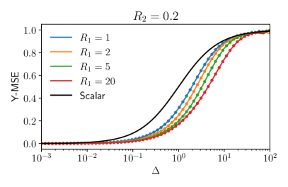
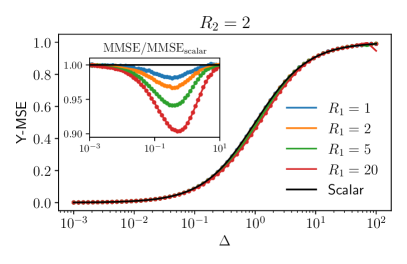
Figure 1: Overview of the behaviour of the MMSE for the Gaussian factorized priors. In each plot, colored lines denote the analytical MMSE Eq. 10, colored dots the empirical MMSE estimated on single instances at size $m=2000$ while the black line shows the MMSE of scalar denoising. In all panels we observe a perfect agreement between theory and simulations. The left panel shows the dependence of the MMSE on $R_{1}$ in the under-complete case $R_{2}<1$: we observe that the MMSE greatly improves as $R_{1}$ grows. The right shows the same in the over-complete case: the dependence on $R_{1}$ in this regime is very small, and it is highlighted in the inset where the y axis has been rescaled using the $R_{2}\to\infty$ limit of the MMSE, that of scalar denoising.

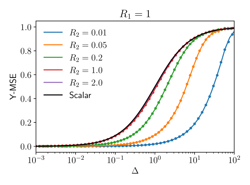
Figure 2: Limiting behaviour of the MMSE for $R_{2}\to\infty$. At fixed $R_{1}$, the plot show convergence to the scalar denoising limit as $R_{2}\to\infty$. Colored lines denote the analytical MMSE Eq. 10, colored dots the empirical MMSE estimated on single instances at size $m=2000$ and black lines denote the scalar denoising $\operatorname{MMSE}_{\rm scalar}=\Delta/(\Delta+1)$.

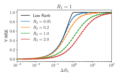
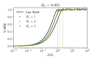
Figure 3: Limiting behaviour of the MMSE for $R_{2}\to 0$. In each plot, colored lines denote the analytical MMSE Eq. 10, colored dots the empirical MMSE estimated on single instances at size $m=2000$ and black lines denote the low-rank limiting behaviour. We rescaled the horizontal axis to better highlight convergence to the limit. The left panel shows, at fixed $R_{1}$, convergence to the low-rank limit as $R_{2}\to 0$. The right shows, at fixed small $R_{2}$, the dependence on $R_{1}$ of the low-rank behaviour. Vertical lines highlight the critical value $R_{2}\Delta_{c}=\sqrt{R_{1}}$ at which the MMSE changes behaviour: above this threshold, no denoising is possible at low-rank.

1.4 Related works

Spectral denoisers for covariance matrices have been used extensively in finance, as in Ledoit and Wolf [2012], Bun et al. [2016, 2017]. Very recently Benaych-Georges et al. [2021] proposed an algorithm to denoise cross correlation matrices that is in spirit similar to the one we propose, with a crucial difference. In our setting, the signal matrix ${\boldsymbol{S}}^{*}={\boldsymbol{F}}{\boldsymbol{X}}$ is corrupted by a noisy channel, and the objective is to get rid of the noise. In their setting, they are given two correlated datasets ${\boldsymbol{F}}$ and ${\boldsymbol{X}}$, and the objective is to estimate their theoretical cross-covariance, which is a non-trivial task when the number of observations $r$ is comparable with the dimensions $m,p$. Qualitatively, in their setting the noise is a finite-size effect due to a finite sample-to-dimension ratio. The algorithm of Benaych-Georges et al. [2021] is also a rotationally invariant estimator, i.e. one where every eigenvalue is rescaled by a function, though their function is different from our Eq. 7.

Our proof strategy is also different from the one used in the works cited above: we derive our estimator from a free entropy approach rooted in statistical physics, which allows us to predict a priori the MMSE between the signal and the denoised sample. This approach was presented for extensive-rank matrix denoising in Schmidt [2018], Maillard et al. [2021], Barbier and Macris [2021]. In Maillard et al. [2021] the denoising problem was solved for square symmetric priors, obtaining the already known denoiser of Bun et al. [2017] and predicting its theoretical MMSE. The authors there study denoising in the context of a high-temperature expansion approach to matrix factorization. We extend their analysis to non-symmetric rectangular priors, and we find the symmetric-case denoiser as a special case of our optimal denoiser. In Barbier and Macris [2021], the computation of the denoising free entropy is presented as a stepping stone towards the computation of minimum mean-squared error of extensive rank matrix factorization aiming to go beyond the rotationally invariant priors on ${\boldsymbol{S}}$. The mathematical challenge in Barbier and Macris [2021] is linked to finding closed forms for the corresponding HCIZ integral in the limit of high dimension. The main point of their work is a closed form expression that presents a conjecture for the free entropy for matrix denoising and factorization in terms of some spectral quantities and the HCIZ integral. Evaluating this formula would require to compute HCIZ in a generic setting, which as far as we know is for the moment out of reach. If the conjecture of Barbier and Macris [2021] is correct then our results can be seen as an explicit evaluation of their formula for the special case of rotationally invariant priors on ${\boldsymbol{S}}$. Note, however, that even checking that indeed for rotationally invariant priors the conjecture of Barbier and Macris [2021] recovers our results is so far open.

The asymptotic behaviour of HCIZ integrals — symmetric and rectangular — has been studied extensively in the literature, both in the context of free probability (Guionnet and Zeitouni [2002], Guionnet and Huang [2021]) and by the statistical physics community (Matytsin [1994], Zinn-Justin and Zuber [2003], Collins et al. [2020]), yet explicit forms in special cases were considered only sporadically Bun et al. [2014]. To the best of our knowledge, the explicit form given in Eq. 12 has not been presented elsewhere.

2 Analytical derivation of the optimal estimator and its performance

As we briefly discussed in the introduction, both the optimal estimator and its MSE are related to properties of the posterior distribution Eq. 8 and its partition function Eq. 9. Moreover, both can be derived from the knowledge of the free entropy $\Phi_{{\boldsymbol{Y}}}\equiv\log(\mathcal{Z}_{{\boldsymbol{Y}}})/(mp)$. Indeed, one can check that the posterior average, i.e. the optimal estimator, is given by

$$\boldsymbol{\hat{S}}({\boldsymbol{Y}})_{i\mu}=\int d{\boldsymbol{S}}\,{\boldsymbol{S}}_{i\mu}P({\boldsymbol{S}}\mid{\boldsymbol{Y}})={\boldsymbol{Y}}_{i\mu}+\frac{\Delta}{\sqrt{mp}}\frac{1}{\mathcal{Z}_{{\boldsymbol{Y}}}}\frac{\partial\mathcal{Z}_{{\boldsymbol{Y}}}}{\partial{\boldsymbol{Y}}_{i\mu}}={\boldsymbol{Y}}_{i\mu}+\Delta\sqrt{mp}\frac{\partial\Phi_{{\boldsymbol{Y}}}}{\partial{\boldsymbol{Y}}_{i\mu}}\,,$$ (13)

by computing explicitly the derivative $\partial_{{\boldsymbol{Y}}}\mathcal{Z}_{{\boldsymbol{Y}}}$ starting from Eq. 9. For the MMSE Eq. 4, by the I-MMSE theorem Guo et al. [2005], we have

$$\operatorname{MMSE}=\Delta+2\Delta^{2}\partial_{\Delta}\mathbb{E}_{{\boldsymbol{Y}}}\left[\Phi_{{\boldsymbol{Y}}}\right]\,.$$ (14)

A sketch of the derivation of Eq. 14 with our specific normalizations and notations is given in Appendix D. The main focus of the section will be to compute the free entropy $\Phi_{{\boldsymbol{Y}}}$ in the high-dimensional limit.

2.1 Asymptotics of the free entropy $\Phi_{{\boldsymbol{Y}}}$

To compute the free entropy, we start by performing a change of variable from ${\boldsymbol{S}}$ to its singular value decomposition ${\boldsymbol{S}}={\boldsymbol{U}}{\boldsymbol{T}}{\boldsymbol{V}}$ in Eq. 9, with ${\boldsymbol{U}}\in\mathcal{O}({m})$, ${\boldsymbol{V}}\in\mathcal{O}({p})$ and diagonal ${\boldsymbol{T}}\in\mathbb{R}_{+}^{m\times p}$ (recall that without loss of generality we took $m\leq p$). We will denote the singular values as ${\boldsymbol{T}}_{ll}=T_{l}$ for $l=1,\dots,m$. As usual — see Anderson et al. [2010] for example — the Jacobian of the change of variable involves the Vandermonde determinant of the squared singular values ${\boldsymbol{T}}^{2}$, $\Delta({\boldsymbol{T}}^{2})=\prod_{i<j}^{m}(T_{i}^{2}-T_{j}^{2})$, as well as an additional term involving the product of singular values

$$\begin{split}\mathcal{Z}_{{\boldsymbol{Y}}}&=\Delta^{-\frac{mp}{2}}\int\mu_{{m}}({d{\boldsymbol{U}}})\,\mu_{{p}}({d{\boldsymbol{V}}})\,d{\boldsymbol{T}}\,P_{\rm signal}({\boldsymbol{T}})|\Delta({\boldsymbol{T}}^{2})|\prod_{l=1}^{m}T_{l}^{p-m}\\ &\quad\times\exp\left[-\frac{\sqrt{mp}}{2\Delta}\left(\sum_{l=1}^{m}T^{2}_{l}+\operatorname{Tr}({\boldsymbol{Y}}{\boldsymbol{Y}}^{T})\right)\right]\exp\left[\frac{\sqrt{mp}}{\Delta}\operatorname{Tr}\left({\boldsymbol{U}}{\boldsymbol{T}}{\boldsymbol{V}}{\boldsymbol{Y}}^{T}\right)\right]\\ &=\Delta^{-\frac{mp}{2}}\exp\left[-\frac{\sqrt{mp}}{2\Delta}\operatorname{Tr}\left({\boldsymbol{Y}}{\boldsymbol{Y}}^{T}\right)\right]\int d{\boldsymbol{T}}\,P_{\rm signal}({\boldsymbol{T}})|\Delta({\boldsymbol{T}}^{2})|\prod_{l=1}^{m}T_{l}^{(R_{1}-1)m}\\ &\quad\times\exp\left[-\frac{\sqrt{mp}}{2\Delta}\sum_{l=1}^{m}T^{2}_{l}\right]\mathcal{I}_{m}\left({\boldsymbol{T}},{\boldsymbol{Y}};\frac{\sqrt{R}_{1}}{\Delta}\right)\,.\end{split}$$ (15)

where $\mu_{{m}}({\cdot})$ is the uniform measure on the orthogonal group in dimension $m$ and where we recognized that the integral over rotation matrices reduces to the rectangular HCIZ integral defined in Eq. 11. Notice that we used the rotational invariance of the prior to argue that $P_{\rm signal}({\boldsymbol{S}})=P_{\rm signal}({\boldsymbol{T}})$. In the non-rotational invariant case $P_{\rm signal}({\boldsymbol{S}})$ would also depend on the singular vectors of ${\boldsymbol{S}}$.

To move forward, we notice that all quantities appearing in the integral depend on the singular values matrix ${\boldsymbol{T}}$ through its symmetrized empirical singular value density $\hat{\sigma}({{{\boldsymbol{T}}}})$, and that they have finite asymptotic limit in the exponential scale $\exp(m^{2})$. Then, we change integration variables from the ”$m$-dimensional” empirical density $\hat{\sigma}({{{\boldsymbol{T}}}})$ to a generic probability density $\rho$: we argue in Appendix E that in the large $m$ limit this change introduces only a term in the exponential scale $\exp(m)$, which is thus subleading with respect to the original integrand and can be discarded. Finally, we use Laplace’s method to observe that the integral concentrates in the scale $\exp(m^{2})$ onto the value of the integrand at a deterministic density $\rho^{*}$; Nishimori identities Nishimori [1980] guarantee then that $\rho^{*}=\hat{\sigma}_{{{\boldsymbol{S}}^{*}}}$ (see also Barbier and Macris [2021], Maillard et al. [2021] for more discussions of this phenomenon). Thus, by taking the leading asymptotic order of all terms and disregarding all finite-size corrections and all constant terms depending only on $R_{1}$

$$\begin{split}\Phi_{{\boldsymbol{Y}}}&=-\frac{1}{2}\log\Delta+\frac{1}{mp}\log P_{\rm signal}[\hat{\sigma}_{{{\boldsymbol{S}}^{*}}}]-\frac{1}{2\Delta\sqrt{R_{1}}}\operatorname{Var}[\hat{\sigma}_{{{\boldsymbol{S}}^{*}}}]+\frac{1}{R_{1}}\Sigma\left[\hat{\sigma}_{{{\boldsymbol{S}}^{*}}}\right]\\ &\quad+\frac{R_{1}-1}{R_{1}}\Lambda\left[\hat{\sigma}_{{{\boldsymbol{S}}^{*}}}\right]-\frac{1}{2\Delta\sqrt{R_{1}}}\operatorname{Var}[\hat{\sigma}({{{\boldsymbol{Y}}}})]+\frac{1}{2R_{1}}I_{R_{1}}\left[\hat{\sigma}_{{{\boldsymbol{S}}^{*}}},\hat{\sigma}({{{\boldsymbol{Y}}}});\frac{\sqrt{R_{1}}}{\Delta}\right]\end{split}$$ (16)

where $\operatorname{Var}[\sigma]=\int dx\,\sigma(x)x^{2}$, $\Sigma[\sigma]=\mathchoice{{\vbox{\hbox{$\textstyle-$}}\kern-4.86108pt}}{{\vbox{\hbox{$\scriptstyle-$}}\kern-3.25pt}}{{\vbox{\hbox{$\scriptscriptstyle-$}}\kern-2.29166pt}}{{\vbox{\hbox{$\scriptscriptstyle-$}}\kern-1.875pt}}\!\int dx\,dy\,\sigma(x)\sigma(y)\log|x-y|$ and $\Lambda[\sigma]=\mathchoice{{\vbox{\hbox{$\textstyle-$}}\kern-4.86108pt}}{{\vbox{\hbox{$\scriptstyle-$}}\kern-3.25pt}}{{\vbox{\hbox{$\scriptscriptstyle-$}}\kern-2.29166pt}}{{\vbox{\hbox{$\scriptscriptstyle-$}}\kern-1.875pt}}\!\int dx\,\sigma(x)\log|x|$, and $\hat{\sigma}_{{{\boldsymbol{S}}^{*}}}$ is the asymptotic symmetrized singular value densities of ${\boldsymbol{S}}^{*}$. $\hat{\sigma}({{{\boldsymbol{Y}}}})$ instead is the symmetrized empirical density of singular values of the fixed instance of the observation ${\boldsymbol{Y}}$. All dashed integrals are regularized as detailed in Appendix A.

In Eq. 16 we took the high-dimensional limit of the prior term $(mp)^{-1}\log P_{\rm signal}({\boldsymbol{T}})$ in a rather uncontrolled way. Treating the limit rigorously is delicate, see for example the discussions in [Barbier and Macris, 2021, Section II.C], but brings no surprises for non-pathological priors — for example, the factorized priors in the symmetric version of our problem Maillard et al. [2021]. As mentioned at the start of the section, all quantities we are interested in depend on derivatives of the free entropy with respect to $\Delta$ or to ${\boldsymbol{Y}}$, and the prior term brings no contribution at all in these cases. For this reason, we do not treat it in detail.

We will show in Section 4 that at leading order

$$\begin{split}I_{R_{1}}\left[\hat{\sigma}_{{{\boldsymbol{S}}^{*}}},\hat{\sigma}({{{\boldsymbol{Y}}}});\frac{\sqrt{R_{1}}}{\Delta}\right]&=C_{R_{1}}+R_{1}\log\Delta+\frac{\sqrt{R_{1}}}{\Delta}\operatorname{Var}[\hat{\sigma}_{{{\boldsymbol{S}}^{*}}}]+\frac{\sqrt{R_{1}}}{\Delta}\operatorname{Var}[\hat{\sigma}({{{\boldsymbol{Y}}}})]\\ &\quad-2(R_{1}-1)\Lambda[\hat{\sigma}({{{\boldsymbol{Y}}}})]-2\Sigma[\hat{\sigma}({{{\boldsymbol{Y}}}})]\end{split}$$ (17)

for some constant $C_{R_{1}}$ depending only on $R_{1}$. The asymptotic free entropy thus equals

$$\begin{split}\Phi_{{\boldsymbol{Y}}}&=\text{const}(R_{1})+\frac{1}{mp}\log P_{\rm signal}[\hat{\sigma}_{{{\boldsymbol{S}}^{*}}}]+\frac{1}{R_{1}}\Sigma\left[\hat{\sigma}_{{{\boldsymbol{S}}^{*}}}\right]+\frac{R_{1}-1}{R_{1}}\Lambda\left[\hat{\sigma}_{{{\boldsymbol{S}}^{*}}}\right]\\ &\quad-\frac{1}{R_{1}}\Sigma\left[\hat{\sigma}({{{\boldsymbol{Y}}}})\right]-\frac{R_{1}-1}{R_{1}}\Lambda[\hat{\sigma}({{{\boldsymbol{Y}}}})]\,,\end{split}$$ (18)

where $\text{const}(R_{1})$ gathers all constants depending on $R_{1}$ that we did not trat explicitly, namely the constant in the HCIZ asymptotics and the constant in the intial SVD change of variable. Notice that only the last two terms depend either on ${\boldsymbol{Y}}$ or on $\Delta$ (through the spectral properties of ${\boldsymbol{Y}}$).

2.2 Explicit form of the MMSE and the optimal estimator

The MMSE can be computed directly by combining Eq. 14 with Eq. 18, obtaining

$$\begin{split}\operatorname{MMSE}=\Delta-2\Delta^{2}\frac{\partial}{\partial\Delta}\mathbb{E}_{{\boldsymbol{Y}}}\left[\frac{1}{R_{1}}\Sigma[\hat{\sigma}({{{\boldsymbol{Y}}}})]+\frac{R_{1}-1}{R_{1}}\Lambda[\hat{\sigma}({{{\boldsymbol{Y}}}})]\right]\,.\end{split}$$ (19)

Thanks to the concentration of spectral densities in the high-dimensional limit, the average over ${\boldsymbol{Y}}$ can be performed directly by substituting the empirical symmetrized singular value density $\hat{\sigma}({{{\boldsymbol{Y}}}})$ of the specific instance of the observation ${\boldsymbol{Y}}$ with the asymptotic singular value density $\hat{\sigma}_{{{\boldsymbol{Y}}}}$ of the observation, which is a deterministic quantity: it depends only on the statistical properties of ${\boldsymbol{Y}}$, and not on its specific value. Thus, we obtain Section 1.2.

To compute the explicit form of the optimal estimator, we start from Eq. 13 and notice that the free entropy depends only on spectral properties of the actual instance of the observation ${\boldsymbol{Y}}$. Thus, the derivative of the free entropy w.r.t. one component of ${\boldsymbol{Y}}$ can be decomposed on the eigenvalues of ${\boldsymbol{Y}}$ as follows

$$\boldsymbol{\hat{S}}({\boldsymbol{Y}})_{i\mu}={\boldsymbol{Y}}_{i\mu}+\Delta\sqrt{mp}\frac{\partial\Phi_{{\boldsymbol{Y}}}}{\partial{\boldsymbol{Y}}_{i\mu}}={\boldsymbol{Y}}_{i\mu}+\Delta\sqrt{mp}\sum_{l=1}^{m}\frac{\partial\Phi_{{\boldsymbol{Y}}}}{\partial y_{l}}\frac{\partial y_{l}}{\partial{\boldsymbol{Y}}_{i\mu}}\,,$$ (20)

where in the last passage we called $\{y_{i}\}_{i=1}^{m}$ the singular values of ${\boldsymbol{Y}}$.

To compute the derivative, we use a variant of the Hellman-Feynman theorem Cohen-Tannoudji et al. [1977]. The Hellman-Feynman theorem considers a symmetric matrix depending on a parameter, and relates the derivative of an eigenvalue of the matrix with respect to that parameter with the derivative of the matrix itself. In Appendix F we show that the Hellman-Feynman theorem can be adapted to the case of rectangular matrices and singular values, and in particular we show that $\partial_{\lambda}y=u^{T}\cdot\partial_{\lambda}{{\boldsymbol{M}}}\cdot v$, if ${\boldsymbol{M}}$ is a matrix, $y$ one of its singular values, $u$ and $v$ the corresponding left and right singular vectors, and all these quantities depend on a parameter $\lambda$.

To compute $\partial y_{l}/\partial{\boldsymbol{Y}}_{i_{0}\mu_{0}}$ we need to perturb the original matrix ${\boldsymbol{Y}}$ as ${\boldsymbol{Y}}(\lambda)_{\mu i}={\boldsymbol{Y}}_{i\mu}+\lambda\delta_{ii_{0}}\delta_{\mu\mu_{0}}$ so that (here $u^{l}$ and $v^{l}$ are the left and right singular values of ${\boldsymbol{Y}}$ corresponding to the $l$-th singular vector)

$$\begin{split}\frac{\partial y_{l}}{\partial{\boldsymbol{Y}}_{i_{0}\mu_{0}}}&=\frac{\partial y_{l}}{\partial\lambda}=(u^{l})^{T}\cdot\partial_{\lambda}{\boldsymbol{Y}}(\lambda)\cdot v^{l}=\sum_{i,\mu=1}^{m,p}u_{i}^{l}\delta_{ii_{0}}\delta_{\mu\mu_{0}}v^{l}_{\mu}=u_{i_{0}}^{l}v_{\mu_{0}}^{l}\,.\end{split}$$ (21)

For clarity, $u_{i}^{l}$ is the i-th component of the left singular vector corresponding to the $l$-th singular value, and similarly for $v_{\mu}^{l}$. Thus

$$\left\langle{\boldsymbol{S}}_{i\mu}\right\rangle={\boldsymbol{Y}}_{i\mu}+\Delta\sqrt{mp}\sum_{l=1}^{m}\frac{\partial\Phi_{{\boldsymbol{Y}}}}{\partial y_{l}}u^{l}_{i}v^{l}_{\mu}=\sum_{l=1}^{m}\left[y_{l}+\Delta\sqrt{mp}\frac{\partial\Phi_{{\boldsymbol{Y}}}}{\partial y_{l}}\right]u^{l}_{i}v^{l}_{\mu}=\sum_{l=1}^{m}\xi(y_{l})u^{l}_{i}v^{l}_{\mu}\,,$$ (22)

where we used that ${\boldsymbol{Y}}_{i\mu}=\sum_{l=1}^{m}y_{l}u^{l}_{i}v^{l}_{\mu}$ by definition of SVD and we introduced the spectral denoising function $\xi(y)$. This proves the first claim of Section 1.2, i.e. that the optimal denoiser is diagonal in the bases of left and right singular vectors of the observation ${\boldsymbol{Y}}$.

To obtain an explicit form for the spectral denoising function $\xi$, we need to compute $\partial\Phi_{{\boldsymbol{Y}}}/\partial y_{l}$. For this, we consider the part of the free entropy depending on ${\boldsymbol{Y}}$, call it $\Psi_{{\boldsymbol{Y}}}$, in the discrete setting (all following equalities are intended at leading order for large $m$), i.e.

$$\begin{split}\Psi_{{\boldsymbol{Y}}}&=-\frac{R_{1}-1}{R_{1}}\frac{1}{m}\sum_{l:y_{l}\neq 0}\log|y_{l}|-\frac{1}{R_{1}}\frac{1}{m^{2}}\sum_{l\neq l^{\prime}}\log|y_{l}-y_{l^{\prime}}|\,,\end{split}$$ (23)

so that

$$\begin{split}\sqrt{mp}\frac{\partial\Psi_{{\boldsymbol{Y}}}}{\partial y_{l}}&=-\frac{R_{1}-1}{y_{l}\sqrt{R_{1}}}-\frac{2}{\sqrt{R_{1}}}\frac{1}{m}\sum_{k}\frac{1}{y_{l}-y_{k}}=-\frac{1}{\sqrt{R_{1}}}\frac{R_{1}-1}{y_{l}}-\frac{2}{\sqrt{R_{1}}}\mathchoice{{\vbox{\hbox{$\textstyle-$}}\kern-4.86108pt}}{{\vbox{\hbox{$\scriptstyle-$}}\kern-3.25pt}}{{\vbox{\hbox{$\scriptscriptstyle-$}}\kern-2.29166pt}}{{\vbox{\hbox{$\scriptscriptstyle-$}}\kern-1.875pt}}\!\int dx\,\frac{\hat{\sigma}({{{\boldsymbol{Y}}}})(x)}{y_{l}-x}\,,\end{split}$$ (24)

and the spectral denoising function is finally given by

$$\xi(y)=y-\frac{2\Delta}{\sqrt{R_{1}}}\left[\frac{R_{1}-1}{2y}+\mathchoice{{\vbox{\hbox{$\textstyle-$}}\kern-4.86108pt}}{{\vbox{\hbox{$\scriptstyle-$}}\kern-3.25pt}}{{\vbox{\hbox{$\scriptscriptstyle-$}}\kern-2.29166pt}}{{\vbox{\hbox{$\scriptscriptstyle-$}}\kern-1.875pt}}\!\int d\zeta\,\frac{\hat{\sigma}({{{\boldsymbol{Y}}}})(\zeta)}{y-\zeta}\right]\,.$$ (25)

We thus recover the second part of Section 1.2, i.e. the expression for the denoising function $\xi$, by invoking once again concentration of spectral densities, so that $\hat{\sigma}({{{\boldsymbol{Y}}}})$ can be safely substituted by its asymptotic deterministic counterpart $\hat{\sigma}_{{{\boldsymbol{Y}}}}$ in the high-dimensional limit.

3 Specific priors

In this section we provide all the ingredients needed to specialize Section 1.2 and Section 1.2 to specific choices of rotationally-invariant priors. We then analyze in detail the case of the Gaussian factorized matrix prior defined in Eq. 2.

3.1 General remarks

The two main ingredients needed to make our results explicit for a specific form of the prior are the symmetrized singular value density of the observation $\hat{\sigma}_{{{\boldsymbol{Y}}}}$ and its Hilbert transform $\mathcal{H}[\hat{\sigma}_{{{\boldsymbol{Y}}}}](y)=\frac{1}{\pi}\mathchoice{{\vbox{\hbox{$\textstyle-$}}\kern-4.86108pt}}{{\vbox{\hbox{$\scriptstyle-$}}\kern-3.25pt}}{{\vbox{\hbox{$\scriptscriptstyle-$}}\kern-2.29166pt}}{{\vbox{\hbox{$\scriptscriptstyle-$}}\kern-1.875pt}}\!\int d\zeta\,\hat{\sigma}_{{{\boldsymbol{Y}}}}(\zeta)/(y-\zeta)$. Now we show how to compute them analytically.

The first ingredient needed is the so-called Stieltjes transform of the symmetrized singular value density $\hat{\sigma}_{{{\boldsymbol{A}}}}(x)$, i.e.

$$g_{{\boldsymbol{A}}}(z)=\int dx\frac{\hat{\sigma}_{{{\boldsymbol{A}}}}(x)}{z-x}\quad\text{for}\quad z\in\mathbb{C}\setminus\operatorname*{supp}{\hat{\sigma}_{{{\boldsymbol{A}}}}}\,,$$ (26)

where $\operatorname*{supp}{\hat{\sigma}_{{{\boldsymbol{A}}}}}$ denotes the support $\hat{\sigma}_{{{\boldsymbol{A}}}}$. Indeed, one can show that (see for example Potters and Bouchaud [2020])

$$\hat{\sigma}_{{{\boldsymbol{A}}}}(x)=\frac{1}{\pi}\lim_{\epsilon\to 0^{+}}\Im g_{{\boldsymbol{A}}}(x-i\epsilon)\quad\text{and}\quad\mathchoice{{\vbox{\hbox{$\textstyle-$}}\kern-4.86108pt}}{{\vbox{\hbox{$\scriptstyle-$}}\kern-3.25pt}}{{\vbox{\hbox{$\scriptscriptstyle-$}}\kern-2.29166pt}}{{\vbox{\hbox{$\scriptscriptstyle-$}}\kern-1.875pt}}\!\int dx\,\frac{\hat{\sigma}_{{{\boldsymbol{A}}}}(x)}{y-x}=\lim_{\epsilon\to 0^{+}}\Re g_{{\boldsymbol{A}}}(x-i\epsilon)$$ (27)

where the second equality follows from Kramers–Kronig relations (Jackson [1975]). Thus, from the knowledge of $g_{{\boldsymbol{A}}}$ one can recover both the symmetrized singular value density and the corresponding Hilbert transform, obtaining all the ingredients needed to make the optimal estimator Eq. (6) and the MMSE Eq. (10) explicit for a given prior. Notice that, while in the following we will focus on cases in which $g_{{\boldsymbol{A}}}$ can be computed analytically, our algorithm can be in principle applied to any rotationally-invariant ensemble of random matrices ${\boldsymbol{A}}$ by sampling a large matrix and computing its singular values to estimate $g_{{\boldsymbol{A}}}$ as in Ledoit and Péché [2011].

Thus, the questions shifts to how to compute the Stieltjes transform of $\hat{\sigma}_{{{\boldsymbol{A}}}}$, which in turn entails two sub-problems: determining the Stieltjes transform of the prior $g_{{\boldsymbol{S}}^{*}}(z)$, and then adding the effect of the noise.

In order to compute the Stieltjes transform of the prior, we consider the matrix ${\boldsymbol{A}}{\boldsymbol{A}}^{T}$. Indeed, if ${\boldsymbol{A}}$ has SVD ${\boldsymbol{A}}={\boldsymbol{U}}{\boldsymbol{B}}{\boldsymbol{V}}$ with diagonal ${\boldsymbol{B}}$, then ${\boldsymbol{A}}{\boldsymbol{A}}^{T}={\boldsymbol{U}}{\boldsymbol{B}}{\boldsymbol{B}}^{T}{\boldsymbol{U}}^{T}$, from which we see that there is a one-to-one correspondence between singular values of ${\boldsymbol{A}}$ and eigenvalues of ${\boldsymbol{A}}{\boldsymbol{A}}^{T}$. Namely the former are the positive square roots of the latter (notice that ${\boldsymbol{A}}{\boldsymbol{A}}^{T}$ is symmetric and positive semi-definite). This eigenvalues-singular values relations has a consequence on the corresponding Stieltjes transforms. Indeed

$$g_{{\boldsymbol{A}}}(z)=\int dx\,\frac{\hat{\sigma}_{{{\boldsymbol{A}}}}(x)}{z-x}=\int_{0}^{\infty}dx\,\frac{2z\,\sigma_{{{\boldsymbol{A}}}}(x)}{z^{2}-x^{2}}=\int_{0}^{\infty}d\lambda\,\frac{z\,\sigma_{{{\boldsymbol{A}}{\boldsymbol{A}}^{T}}}(\lambda)}{z^{2}-\lambda}=zg_{{\boldsymbol{A}}{\boldsymbol{A}}^{T}}(z^{2})$$ (28)

where $\sigma_{{{\boldsymbol{A}}{\boldsymbol{A}}^{T}}}$ is the usual spectral density of ${\boldsymbol{A}}{\boldsymbol{A}}^{T}$. Thus, Eq. 28 links the Stieltjes transform of the singular value density of a rectangular matrix, which is in principle a very generic and non-trivial quantity to compute, to the Stieltjes transform of the eigenvalue density of a symmetric square matrix, for which many explicit analytical and numerical results already exist in the literature Potters and Bouchaud [2020].

Notice that the procedure just described is of no help in order to add the noise: in fact, $({\boldsymbol{A}}+{\boldsymbol{Z}})({\boldsymbol{A}}+{\boldsymbol{Z}})^{T}$ is a sum of products of matrices that are not independent (free) between each other. Thus, usual free probability techniques based on the $\mathcal{R}$ or $\mathcal{S}$ transforms and free convolution of symmetric matrices would fail to treat this problem.

In order to add the effect of the noise, one needs rectangular free probability techniques. We do not enter into the details here: we refer the interested reader to Benaych-Georges [2009]. The underlying idea is not different from what happens in the more conventional symmetric case: there exists a functional transform of the Stieltjes transform, the rectangular $\mathcal{R}$ transform, that linearizes the sum of random matrices, i.e. $\mathcal{R}[g_{{\boldsymbol{A}}}]+\mathcal{R}[g_{{\boldsymbol{B}}}]=\mathcal{R}[g_{{\boldsymbol{A}}+{\boldsymbol{B}}}]$ whenever the random matrices ${\boldsymbol{A}}$ and ${\boldsymbol{B}}$ are mutually free. Thus, one can access the Stieltjes transform of the sum by computing two direct $\mathcal{R}$ transforms, and one inverse $\mathcal{R}$ transform. In practice, the computation of the rectangular $\mathcal{R}$ transform entails the numerical estimation of functional inverses as soon as one departs from the simplest case of matrices with i.i.d. Gaussian entries. For this reason, in the special case of factorized priors Eq. 2, we will not pursue this very general strategy. Instead, in Section 3.3 we will adapt the results of Pennington and Worah [2017], Louart et al. [2018], which are easier to implement numerically.

As a final remark, notice that the Stieltjes transform scales under a rescaling of ${\boldsymbol{A}}$ as $g_{c{\boldsymbol{A}}}(z)=g_{{\boldsymbol{A}}}\left(z/c\right)/c$. This will be useful to deal with the many constant terms appearing in our computations.

3.2 Symmetric priors

The case of symmetric priors has already been treated originally in Bun et al. [2016], and more recently in Maillard et al. [2021] with techniques akin to ours. In particular, with a symmetric prior one can repeat our analysis using eigenvalue densities instead of singular value densities. For positive semi-definite symmetric priors, it is immediate to see that our results reduce to those of Bun et al. [2016], Maillard et al. [2021], as singular values coincide with eigenvalues in this case. For generic symmetric priors, singular values are the absolute values of eigenvalues, and thus the singular value density is simply given by the symmetrized spectral density.

3.3 The case of Gaussian factorized prior

The prior we would like to focus our attention on is given by the model of Gaussian extensive-rank factorized signals defined in Eq. 2. As argued in Section 3.1, we need a way to compute the Stieltjes transform of the observation ${\boldsymbol{Y}}$ for this specific prior in order to have access to $\hat{\sigma}_{{{\boldsymbol{Y}}}}$ — to numerically compute the integrals in the MMSE formula Eq. 10 — and its Hilbert transform — to be able to perform actual denoising on given instances of ${\boldsymbol{Y}}$ using Eq. 6.

To this end, we generalize the results given in Pennington and Worah [2017]. There, the authors study the spectrum of ${\boldsymbol{C}}=f({\boldsymbol{F}}{\boldsymbol{X}})f({\boldsymbol{F}}{\boldsymbol{X}})^{T}$, where $f$ is a component-wise non-linearity and ${\boldsymbol{F}},{\boldsymbol{X}}$ matrices with i.i.d. Gaussian entries. They show that the Stieltjes transform of the spectral density of ${\boldsymbol{C}}$ satisfies a degree-four algebraic equation depending only on the aspect-ratio $R_{1}$, the rank parameter $R_{2}$ and two Gaussian moments of $f$, $\eta=\int Dzf(z)^{2}$ and $\zeta=\big{[}\int Dzf^{\prime}(z)\big{]}^{2}$, where $Dz$ denotes integration over a standard Gaussian random variable.

Recall that, thanks to Eq. 28, knowing the Stieltjes transform of the spectral density of ${\boldsymbol{C}}$ is equivalent to knowing that of the singular value density of $f({\boldsymbol{F}}{\boldsymbol{X}})$. Thus, we could compute $g_{{\boldsymbol{Y}}}$ by choosing a noisy function $f(x)=x+z$, where $z$ is a Gaussian random variable (actually, one for each component of the matrix, all i.i.d.). In order to do that, we just need to show that the results of Pennington and Worah [2017] extend to non-deterministic non-linearities — only the deterministic case is considered therein. This happens to be the case: we provide the details of the extension in Appendix G. The only effect of the noise of the non-linearity is a redefinition of the Gaussian moments of $f$, and in particular $\eta_{\rm noisy}=\mathbb{E}_{f}\int Dzf(z)^{2}$ and $\zeta_{\rm noisy}=\mathbb{E}_{f}\left[\int Dzf^{\prime}(z)\right]^{2}$, where $\mathbb{E}_{f}$ denotes averaging over the noise induced by $f$.

Thus, we can safely use the results from Pennington and Worah [2017] to compute the Stieltjes transform of the singular value density of ${\boldsymbol{Y}}$ for Gaussian factorized priors. There is a non-trivial mismatch between our normalizations and those of Pennington and Worah [2017]: to fall-back directly onto their results, we need to choose $f(x)=\sqrt[4]{R_{1}}(x+\sqrt{\Delta}z)$, and set their parameters to $\sigma_{x}=\sigma_{w}=1$, $\phi=R_{2}/R_{1}$ and $\psi=R_{2}$.

With these choices, the Gaussian moments of $f$ are given by $\eta_{\rm noisy}=(1+\Delta)\sqrt{R_{1}}$ and $\zeta_{\rm noisy}=\sqrt{R_{1}}$. The algebraic equation for $g_{{\boldsymbol{Y}}}(z)$ is given by [Pennington and Worah, 2017, SM, Eq. S42-S43] and is reported in Appendix G.

4 Asymptotics of the HCIZ integral

In this section we consider the asymptotics of the rectangular HCIZ presented in Guionnet and Huang [2021] and adapt them to the problem of denoising.

We follow the notations of the paper. In particular, their parameters $\alpha$ and $\beta$ in our case equal $\alpha=R_{1}-1$ and $\beta=1$. The HCIZ integral was defined in Eq. 11, and its asymptotic value is defined as

$$I_{\alpha}[\hat{\sigma}_{{{\boldsymbol{A}}}},\hat{\sigma}_{{{\boldsymbol{B}}}};\lambda]=\lim_{m\to\infty,p=(1+\alpha)m}\frac{2}{m^{2}}\log\mathcal{I}_{m}({\boldsymbol{A}},{\boldsymbol{B}};\lambda)\,,$$ (29)

where $\hat{\sigma}_{{{\boldsymbol{A}},{\boldsymbol{B}}}}$ are the asymptotic symmetrized singular value densities of ${\boldsymbol{A}}$ and ${\boldsymbol{B}}$. Following [Guionnet and Huang, 2021, Theorem 1.1], the asymptotic of the HCIZ integral with parameter $\tau=1$ equals

$$\begin{split}I_{\alpha}\left[\hat{\sigma}_{{{\boldsymbol{A}}}},\hat{\sigma}_{{{\boldsymbol{B}}}};\tau=1\right]&=C_{\alpha}+\operatorname{Var}[\hat{\sigma}_{{{\boldsymbol{A}}}}]-\alpha\Lambda[\hat{\sigma}_{{{\boldsymbol{A}}}}]-\Sigma[\hat{\sigma}_{{{\boldsymbol{A}}}}]+\operatorname{Var}[\hat{\sigma}_{{{\boldsymbol{B}}}}]-\alpha\Lambda[\hat{\sigma}_{{{\boldsymbol{B}}}}]-\Sigma[\hat{\sigma}_{{{\boldsymbol{B}}}}]\\ &\quad-\inf_{\{{\hat{\rho}}_{t}\}_{0\leq t\leq 1}}\left\{\int_{0}^{1}ds\int dx{\hat{\rho}}_{s}(x)\left[v_{s}^{2}(x)+\frac{\pi^{2}}{3}{\hat{\rho}}_{s}^{2}(x)+\frac{\alpha^{2}}{4x^{2}}\right]\right\}\end{split}$$ (30)

where $\operatorname{Var}[\sigma]=\int dx\,\sigma(x)x^{2}$, $\Lambda[\sigma]=\int dx\,\sigma(x)\log|x|$, $\Sigma[\sigma]=\mathchoice{{\vbox{\hbox{$\textstyle-$}}\kern-4.86108pt}}{{\vbox{\hbox{$\scriptstyle-$}}\kern-3.25pt}}{{\vbox{\hbox{$\scriptscriptstyle-$}}\kern-2.29166pt}}{{\vbox{\hbox{$\scriptscriptstyle-$}}\kern-1.875pt}}\!\int dxdy\,\sigma(x)\sigma(y)\log|x-y|$, $C_{\alpha}$ is an unspecified constant depending only on $\alpha$, the infimum is taken over continuous symmetric density valued processes $({\hat{\rho}}_{t}(x))_{0\leq t\leq 1}$ such that ${\hat{\rho}}_{0}(x)=\hat{\sigma}_{{{\boldsymbol{A}}}}$ and ${\hat{\rho}}_{1}(x)=\hat{\sigma}_{{{\boldsymbol{B}}}}$, and where $v_{t}(x)$ is a solution to the continuity equation $\partial_{t}{\hat{\rho}}_{t}(x)+\partial_{x}\left({\hat{\rho}}_{t}(x)v_{t}(x)\right)=0$. We refer the reader to the original work for precise definitions and assumptions over all quantities.

The non-trivial part of Eq. (30), i.e. the optimization problem, is a mass transport problem whose solution interpolates between the singular value densities of the two matrices ${\boldsymbol{A}}$ and ${\boldsymbol{B}}$. This transport problem can be understood as the evolution of a hydrodynamical system, and it can be shown [Menon, 2017, Eq. 4.13] that the resulting density profile ${\hat{\rho}}_{t}(x)$ (i.e. the process at which the infimum is reached) is the symmetrized singular value density of the Dyson Brownian bridge between ${\boldsymbol{A}}$ and ${\boldsymbol{B}}$, i.e. the symmetrized singular value density of the matrix

$${\boldsymbol{X}}(t)=(1-t){\boldsymbol{A}}+t{\boldsymbol{B}}+\sqrt{t(1-t)}{\boldsymbol{W}}$$ (31)

where ${\boldsymbol{W}}$ is a matrix of i.i.d. Gaussian variables with mean zero and variance $1/m$. It can be shown [Guionnet and Huang, 2021, section 4] that the velocity field $v_{t}(x)$ satisfies

$$v_{t}(x)=\pi\mathcal{H}[{\hat{\rho}}_{t}](x)+\frac{\alpha}{2x}+D(x,t)\,,\qquad\mathcal{H}[{\hat{\rho}}](x)=\frac{1}{\pi}\mathchoice{{\vbox{\hbox{$\textstyle-$}}\kern-4.86108pt}}{{\vbox{\hbox{$\scriptstyle-$}}\kern-3.25pt}}{{\vbox{\hbox{$\scriptscriptstyle-$}}\kern-2.29166pt}}{{\vbox{\hbox{$\scriptscriptstyle-$}}\kern-1.875pt}}\!\int dy\,\frac{{\hat{\rho}}(y)}{x-y},$$ (32)

where $\mathcal{H}[\cdot]$ is the Hilbert transform, $\mathchoice{{\vbox{\hbox{$\textstyle-$}}\kern-4.86108pt}}{{\vbox{\hbox{$\scriptstyle-$}}\kern-3.25pt}}{{\vbox{\hbox{$\scriptscriptstyle-$}}\kern-2.29166pt}}{{\vbox{\hbox{$\scriptscriptstyle-$}}\kern-1.875pt}}\!\int$ the Cauchy principal value integral, and $D(x,t)$ is a drift term that ensures that the Brownian motion ends precisely at ${\boldsymbol{B}}$ when $t=1$.

Our aim is to make Eq. 30 explicit in the specific case ${\boldsymbol{B}}-{\boldsymbol{A}}=\kappa{\boldsymbol{W}}$, where ${\boldsymbol{W}}$ is a matrix of i.i.d. Gaussian variables with mean zero and variance $1/m$ and $\kappa$ a positive constant, and for this specific case to extend Eq. 30 to $\tau\neq 1$. One could in principle absorb $\tau$ in the definition of the matrix ${\boldsymbol{A}}$, or ${\boldsymbol{B}}$, or both. We will see shortly that if one wants to make more the asymptotic form of the HCIZ integral explicit in the special case of ${\boldsymbol{B}}={\boldsymbol{A}}$ + Gaussian noise — relevant for the denoising problem — one needs to be careful. In particular, the correct way to absorb $\tau$ is to split it evenly between ${\boldsymbol{A}}$ and ${\boldsymbol{B}}$, by defining ${\boldsymbol{A}}^{\prime}=\sqrt{\tau}{\boldsymbol{A}}$ and ${\boldsymbol{B}}^{\prime}=\sqrt{\tau}{\boldsymbol{B}}$. In this way, the fact that the difference between ${\boldsymbol{B}}^{\prime}$ and ${\boldsymbol{A}}^{\prime}$ is a matrix with Gaussian i.i.d. entries — which, as we will see shortly, is a key property — gets preserved. Thus, $I_{\alpha}[\hat{\sigma}_{{{\boldsymbol{A}}}},\hat{\sigma}_{{{\boldsymbol{A}}+\kappa{\boldsymbol{W}}}};\tau]=I_{\alpha}[\hat{\sigma}_{{{\boldsymbol{A}}^{\prime}}},\hat{\sigma}_{{{\boldsymbol{A}}^{\prime}+\sqrt{\tau}\kappa{\boldsymbol{W}}}};1]$.

Now we notice that in the particular case of ${\boldsymbol{B}}^{\prime}={\boldsymbol{A}}^{\prime}+\sqrt{\tau}\kappa{\boldsymbol{W}}$, Eq. 31 simplifies to a Dyson Brownian motion starting at ${\boldsymbol{A}}$

$$\begin{split}{\boldsymbol{X}}(t)&=(1-t){\boldsymbol{A}}^{\prime}+t({\boldsymbol{A}}^{\prime}+\sqrt{\tau}\kappa{\boldsymbol{W}}_{1})+\sqrt{t(1-t)}{\boldsymbol{W}}_{2}={\boldsymbol{A}}^{\prime}+\sqrt{t}{\boldsymbol{W}}\end{split},$$ (33)

where we summed the two independent (more precisely, free) realizations of the Gaussian matrix ${\boldsymbol{W}}_{1}$ and ${\boldsymbol{W}}_{2}$ by substituting them with a third independent Gaussian matrix ${\boldsymbol{W}}$ and by summing the original variances. We also used the fact that $\sqrt{\tau}\kappa=1$ in the denoising problem; we will discuss the $\sqrt{\tau}\kappa\neq 1$ briefly at the end of this section. Moreover, no drift is needed to impose that ${\boldsymbol{X}}(1)={\boldsymbol{B}}^{\prime}$, so that in Eq. 32 $D(x,t)\equiv 0$ and

$$v_{t}(x)=\pi\mathcal{H}[{\hat{\rho}}_{t}](x)+\frac{\alpha}{2x}\,.$$ (34)

The explicit form Eq. 34 is crucial to make explicit Eq. (30). Indeed, one can show that if Eq. 34 holds, then

$$\begin{split}G(t)&=\Sigma[{\hat{\rho}}_{t}]+\alpha\Lambda[{\hat{\rho}}_{t}]-\int_{0}^{t}ds\int dx{\hat{\rho}}_{s}(x)\left[v_{s}^{2}(x)+\frac{\pi^{2}}{3}{\hat{\rho}}_{s}^{2}(x)+\frac{\alpha^{2}}{4x^{2}}\right]\end{split}$$ (35)

is a constant function of $t$, i.e. $\partial_{t}G(t)=0$, see Appendix H. The fact that $G(0)=G(1)$ allows to explicitly write the dynamical portion of Eq. (30) as

$$\int_{0}^{1}ds\int dx{\hat{\rho}}_{s}(x)\left[v_{s}^{2}(x)+\frac{\pi^{2}}{3}{\hat{\rho}}_{s}^{2}(x)+\frac{\alpha^{2}}{4x^{2}}\right]=\Sigma[\hat{\sigma}_{{{\boldsymbol{A}}^{\prime}}}]+\alpha\Lambda[\hat{\sigma}_{{{\boldsymbol{A}}^{\prime}}}]-\Sigma[\hat{\sigma}_{{{\boldsymbol{B}}^{\prime}}}]-\alpha\Lambda[\hat{\sigma}_{{{\boldsymbol{B}}^{\prime}}}]$$ (36)

in all cases in which ${\boldsymbol{B}}^{\prime}={\boldsymbol{A}}^{\prime}+{\boldsymbol{W}}$ where again ${\boldsymbol{W}}$ is a matrix of i.i.d. Gaussian variables with mean zero and variance $1/m$.

To sum it up and get back to the case of denoising, we have, calling $\tau=\sqrt{R_{1}}/\Delta$,

$$\begin{split}I_{R_{1}}&\left[\hat{\sigma}_{{{\boldsymbol{S}}}},\hat{\sigma}_{{{\boldsymbol{Y}}}};\tau=\frac{\sqrt{R_{1}}}{\Delta}\right]=I_{R_{1}}\left[\hat{\sigma}_{{\sqrt{\tau}{\boldsymbol{S}}}},\hat{\sigma}_{{\sqrt{\tau}{\boldsymbol{S}}+{\boldsymbol{W}}}};1\right]\\ &=C_{R_{1}}+R_{1}\log\Delta+\frac{\sqrt{R_{1}}}{\Delta}\operatorname{Var}[\hat{\sigma}_{{{\boldsymbol{S}}}}]+\frac{\sqrt{R_{1}}}{\Delta}\operatorname{Var}[\hat{\sigma}_{{{\boldsymbol{Y}}}}]-2(R_{1}-1)\Lambda[\hat{\sigma}_{{{\boldsymbol{Y}}}}]-2\Sigma[\hat{\sigma}_{{{\boldsymbol{Y}}}}]\,,\end{split}$$ (37)

where $C_{R_{1}}$ hides all constants that depend exclusively on $R_{1}$, and we used that $\hat{\sigma}_{{\sqrt{\tau}{\boldsymbol{M}}}}(x)=\hat{\sigma}_{{{\boldsymbol{M}}}}\left(x/\sqrt{\tau}\right)/\sqrt{\tau}$.

As a final remark, in the case in which $\sqrt{\tau}\kappa\neq 1$, one can replicate exactly this argument by rescaling the time domain so that ${\boldsymbol{B}}^{\prime}={\boldsymbol{X}}(t=\sqrt{\tau}\kappa)$. This does not change anything, apart from possibly modifying the unspecified constant $C_{R_{1}}$ into a constant $C(R_{1},\sqrt{\tau}\kappa)$. This concludes our derivation of Section 1.2.

Appendix A Details on the regularization of logarithmic integrals

In the expression for the free entropy Eq. 18 and for the MMSE Eq. 10, we have integrals of the form

$$\mathchoice{{\vbox{\hbox{$\textstyle-$}}\kern-4.86108pt}}{{\vbox{\hbox{$\scriptstyle-$}}\kern-3.25pt}}{{\vbox{\hbox{$\scriptscriptstyle-$}}\kern-2.29166pt}}{{\vbox{\hbox{$\scriptscriptstyle-$}}\kern-1.875pt}}\!\int d\lambda\,d\zeta\,\hat{\sigma}_{{{\boldsymbol{Y}}}}(\lambda)\hat{\sigma}_{{{\boldsymbol{Y}}}}(\zeta)\log|\lambda-\zeta|\,, \mathchoice{{\vbox{\hbox{$\textstyle-$}}\kern-4.86108pt}}{{\vbox{\hbox{$\scriptstyle-$}}\kern-3.25pt}}{{\vbox{\hbox{$\scriptscriptstyle-$}}\kern-2.29166pt}}{{\vbox{\hbox{$\scriptscriptstyle-$}}\kern-1.875pt}}\!\int d\lambda\,\hat{\sigma}_{{{\boldsymbol{Y}}}}(\lambda)\log|\lambda|\,,$$ (38)

which have logarithmic divergences, respectively, on the diagonal $\zeta=\lambda$ and at the origin $\lambda=0$. This integrals must be intended as continuum limits of the corresponding discrete expressions for finite sized matrices, i.e.

$$\mathchoice{{\vbox{\hbox{$\textstyle-$}}\kern-4.86108pt}}{{\vbox{\hbox{$\scriptstyle-$}}\kern-3.25pt}}{{\vbox{\hbox{$\scriptscriptstyle-$}}\kern-2.29166pt}}{{\vbox{\hbox{$\scriptscriptstyle-$}}\kern-1.875pt}}\!\int d\lambda\,d\zeta\,\hat{\sigma}_{{{\boldsymbol{Y}}}}(\lambda)\hat{\sigma}_{{{\boldsymbol{Y}}}}(\zeta)\log|\lambda-\zeta|=\lim_{N\to\infty}\frac{1}{N^{2}}\sum_{i,j=1}^{N}\log|\sigma_{i}-\sigma_{j}|\,,$$ (39)

where $\{\sigma_{i}\}$ is the singular spectrum of a size $N$ matrix whose limiting singular value density converges to $\hat{\sigma}_{{{\boldsymbol{Y}}}}$, and

$$\mathchoice{{\vbox{\hbox{$\textstyle-$}}\kern-4.86108pt}}{{\vbox{\hbox{$\scriptstyle-$}}\kern-3.25pt}}{{\vbox{\hbox{$\scriptscriptstyle-$}}\kern-2.29166pt}}{{\vbox{\hbox{$\scriptscriptstyle-$}}\kern-1.875pt}}\!\int d\lambda\,\hat{\sigma}_{{{\boldsymbol{Y}}}}(\lambda)\log|\lambda|=\lim_{N\to\infty}\frac{1}{N^{2}}\sum_{\begin{subarray}{c}i=1\\ \sigma_{i}\neq 0\end{subarray}}^{N}\log|\sigma_{i}|\,.$$ (40)

As the spacing between singular values goes to zero as $N\to\infty$, the correct way to interpret the integrals is, respectively,

$$\mathchoice{{\vbox{\hbox{$\textstyle-$}}\kern-4.86108pt}}{{\vbox{\hbox{$\scriptstyle-$}}\kern-3.25pt}}{{\vbox{\hbox{$\scriptscriptstyle-$}}\kern-2.29166pt}}{{\vbox{\hbox{$\scriptscriptstyle-$}}\kern-1.875pt}}\!\int d\lambda\,d\zeta\,\hat{\sigma}_{{{\boldsymbol{Y}}}}(\lambda)\hat{\sigma}_{{{\boldsymbol{Y}}}}(\zeta)\log|\lambda-\zeta|=\lim_{\epsilon\to 0}\int d\lambda\,d\zeta\,\hat{\sigma}_{{{\boldsymbol{Y}}}}(\lambda)\hat{\sigma}_{{{\boldsymbol{Y}}}}(\zeta)\log|\lambda-\zeta|\,\mathbb{I}(|\zeta-\lambda|>\epsilon)\,,$$ (41)

where $\mathbb{I}(\cdot)$ is the indicator function, and

$$\mathchoice{{\vbox{\hbox{$\textstyle-$}}\kern-4.86108pt}}{{\vbox{\hbox{$\scriptstyle-$}}\kern-3.25pt}}{{\vbox{\hbox{$\scriptscriptstyle-$}}\kern-2.29166pt}}{{\vbox{\hbox{$\scriptscriptstyle-$}}\kern-1.875pt}}\!\int d\lambda\,\hat{\sigma}_{{{\boldsymbol{Y}}}}(\lambda)\log|\lambda|=\lim_{\epsilon\to 0}\int d\lambda\,\hat{\sigma}_{{{\boldsymbol{Y}}}}(\lambda)\log|\lambda|\,\mathbb{I}(|\lambda|>\epsilon)\,.$$ (42)

Appendix B Details of numerical integration of Eq. 10

The only numerical difficulty of the paper is the estimation of the integrals in Eq. 10 in the case of the factorized prior Eq. 2. The integral is performed by quadrature using Simpson’s rule. The function we integrate has a wide support and it peaks around the origin for $R_{2}<1$, so we must have more integration points in this region.

We are left with two sub-problems: estimating the support of $\hat{\sigma}_{{{\boldsymbol{Y}}}}$, and the support of the peak at the origin. The edges of the support of the signal ${\boldsymbol{S}}^{*}$ can be computed exactly following Dupic and Castillo [2014], and in particular their Appendix B, with the parameter conversions

$$\alpha_{1}=R_{2}\,,\alpha_{2}=R_{1}\,$$ (43)

giving a bound $\sigma_{\rm max}({\boldsymbol{S}}^{*})\leq\sigma_{\rm signal}$. An upper-bound on the largest singular value of the full observation ${\boldsymbol{Y}}$ can be obtained by summing the largest support edge computed above and the largest support edge of the Marchenko-Pastur distribution accounting the singular value density of the noise,

$$\sigma_{\rm max}(\sqrt{\Delta}{\boldsymbol{Z}})\leq\frac{\Delta(1+\sqrt{R_{1}})^{2}}{\sqrt{R_{1}}}=\sigma_{\rm noise}\,.$$ (44)

Putting everything together we get:

$$\sigma_{\rm max}({\boldsymbol{Y}})\leq\sigma_{\rm signal}+\sigma_{\rm noise}\,.$$ (45)

The right-most edge of the peak at the origin can be upper bounded empirically by $\sigma_{\rm noise}$. While there are surely tighter bounds, this one allows for reasonable performance in the integration.

Appendix C The MMSE of low-rank denoising

The spiked matrix denoising problem is studied in Lesieur et al. [2017], Miolane [2018]. We are given an observation matrix of the form:

$${\boldsymbol{Y}}=\frac{uv^{T}}{\sqrt{m}}+\sqrt{\Delta}{\boldsymbol{Z}}$$ (46)

where $u\in\mathbb{R}^{m}$, $v\in\mathbb{R}^{p}$ and ${\boldsymbol{Z}}\in\mathbb{R}^{m\times p}$ all have standard Gaussian entries. The MMSE for our problem takes the form [Miolane, 2018, section 2.6]:

$$\operatorname{MMSE}_{\rm spiked}=1-q_{u}q_{v},$$ (47)

where $q_{u}$ and $q_{v}$ are solutions of the fixed point equations:

$$\begin{cases}q_{u}=F\left(\frac{R_{1}q_{v}}{\Delta}\right),\\ q_{v}=F\left(\frac{q_{u}}{\Delta}\right)\,,\end{cases}$$ (48)

with

$$F(q)=\mathbb{E}_{x_{0}^{*},z\sim\mathcal{N}(0,1)}\left[\frac{\int x_{0}^{*}x_{0}e^{x_{0}z\sqrt{q}+x_{0}x_{0}^{*}q-\frac{1}{2}x_{0}^{2}q}dP(x_{0})}{\int e^{x_{0}z\sqrt{q}+x_{0}x_{0}^{*}q-\frac{1}{2}x_{0}^{2}q}dP(x_{0})}\right],$$ (49)

where $P(x)$ is the standard Gaussian PDF. The integral above can be evaluated explicitly, yielding:

$$\begin{cases}q_{u}=\frac{R_{1}q_{v}}{\Delta+R_{1}q_{v}}\,,\\ q_{v}=\frac{q_{u}}{\Delta+q_{u}}\,,\\ \end{cases}$$ (50)

whose solution is

$$\begin{cases}q_{u}=\frac{R_{1}-\Delta^{2}}{\Delta+R_{1}}\,,\quad q_{v}=\frac{R_{1}-\Delta^{2}}{(\Delta+1)R_{1}}\quad&\text{for}\quad 0<\Delta<\sqrt{R_{1}}\,,\\ q_{u}=q_{v}=0\quad&\text{for}\quad\Delta>\sqrt{R_{1}}\,.\\ \end{cases}$$ (51)

There is an undetectable phase for $\Delta>\sqrt{R_{1}}$. In the main text the observation matrix is normalized differently, which is why in Fig. 3 we have the undetectable phase for $\Delta R_{2}>\sqrt{R_{1}}$

Appendix D The I-MMSE theorem

Let us prove Eq. (14), i.e. that

$$\operatorname{MMSE}=\mathbb{E}_{{\boldsymbol{S}}^{*},{\boldsymbol{Y}}}\left[\operatorname{MSE}\left({\boldsymbol{S}}^{*},\left\langle{\boldsymbol{S}}\right\rangle_{{\boldsymbol{Y}}}\right)\right]=\Delta+2\Delta^{2}\partial_{\Delta}\mathbb{E}\left[\Phi_{{\boldsymbol{Y}}}\right]\,,$$ (52)

where in the following $\mathbb{E}_{{\boldsymbol{S}}^{*},{\boldsymbol{Y}}}$ denotes a joint average over ${\boldsymbol{S}}^{*}$ and ${\boldsymbol{Y}}$, and $\left\langle\cdot\right\rangle_{{\boldsymbol{Y}}}$ the posterior average at fixed ${\boldsymbol{Y}}$. We start by expressing the MMSE more explicitly

$$\begin{split}\operatorname{MMSE}&=\frac{1}{\sqrt{mp}}\mathbb{E}_{{\boldsymbol{S}}^{*},{\boldsymbol{Y}}}||{\boldsymbol{S}}^{*}-\left\langle{\boldsymbol{S}}\right\rangle_{{\boldsymbol{Y}}}||_{2}^{2}\\ &=\frac{1}{\sqrt{mp}}\mathbb{E}_{{\boldsymbol{S}}^{*},{\boldsymbol{Y}}}\left[||{\boldsymbol{S}}^{*}||_{2}^{2}+||\left\langle{\boldsymbol{S}}\right\rangle_{{\boldsymbol{Y}}}||_{2}^{2}-2\operatorname{Tr}\left({\boldsymbol{S}}^{*}\left\langle{\boldsymbol{S}}\right\rangle_{{\boldsymbol{Y}}}^{T}\right)\right]\,.\end{split}$$ (53)

Now, we use Nishimori’s identity Nishimori [1980] on the last term, i.e.

$$\mathbb{E}_{{\boldsymbol{S}}^{*},{\boldsymbol{Y}}}[\left\langle g({\boldsymbol{S}}^{*},{\boldsymbol{S}})\right\rangle_{{\boldsymbol{Y}}}]=\mathbb{E}_{{\boldsymbol{Y}}}[\left\langle g({\boldsymbol{S}}_{1},{\boldsymbol{S}}_{2})\right\rangle_{{\boldsymbol{Y}}}]\,,$$ (54)

where ${\boldsymbol{S}}_{1,2}$ are two independent random variables distributed with the posterior distribution, and $g$ a continuous bounded function. In words, under Bayes optimality, the ground-truth is indistinguishable from a sample from the posterior for what concerns averages. In our particular case,

$$\mathbb{E}_{{\boldsymbol{S}}^{*},{\boldsymbol{Y}}}\left[\operatorname{Tr}\left({\boldsymbol{S}}^{*}\left\langle{\boldsymbol{S}}\right\rangle_{{\boldsymbol{Y}}}^{T}\right)\right]=\mathbb{E}_{{\boldsymbol{Y}}}\left[\operatorname{Tr}\left(\left\langle{\boldsymbol{S}}\right\rangle_{{\boldsymbol{Y}}}\left\langle{\boldsymbol{S}}\right\rangle_{{\boldsymbol{Y}}}^{T}\right)\right]=\mathbb{E}_{{\boldsymbol{Y}}}||\left\langle{\boldsymbol{S}}\right\rangle_{{\boldsymbol{Y}}}||_{2}^{2}\,.$$ (55)

Thus

$$\begin{split}\mathbb{E}_{{\boldsymbol{S}}^{*},{\boldsymbol{Y}}}\left[\operatorname{MSE}\left({\boldsymbol{S}}^{*},\left\langle{\boldsymbol{S}}\right\rangle_{{\boldsymbol{Y}}}\right)\right]&=\frac{1}{\sqrt{mp}}\mathbb{E}_{{\boldsymbol{S}}^{*},{\boldsymbol{Y}}}\left[||{\boldsymbol{S}}^{*}||_{2}^{2}-||\left\langle{\boldsymbol{S}}\right\rangle_{{\boldsymbol{Y}}}||_{2}^{2}\right]\,.\end{split}$$ (56)

The second step is to compute $\mathbb{E}_{{\boldsymbol{S}}^{*},{\boldsymbol{Y}}}\left[\partial_{\Delta^{-1}}\Phi_{{\boldsymbol{Y}}}\right]$

$$\begin{split}\mathbb{E}_{{\boldsymbol{S}}^{*},{\boldsymbol{Y}}}\left[\partial_{\Delta^{-1}}\Phi_{{\boldsymbol{Y}}}\right]&=\frac{1}{mp}\mathbb{E}_{{\boldsymbol{S}}^{*},{\boldsymbol{Y}}}\left[\frac{1}{\mathcal{Z}_{{\boldsymbol{Y}}}}\partial_{\Delta^{-1}}\mathcal{Z}_{{\boldsymbol{Y}}}\right]\\ &=\frac{\Delta}{2}-\frac{1}{2\sqrt{mp}}\mathbb{E}_{{\boldsymbol{S}}^{*},{\boldsymbol{Y}}}\left[||{\boldsymbol{S}}^{*}||_{2}^{2}-2||\left\langle{\boldsymbol{S}}\right\rangle_{{\boldsymbol{Y}}}||_{2}^{2}+\left\langle||{\boldsymbol{S}}||_{2}^{2}\right\rangle_{{\boldsymbol{Y}}}-\sqrt{\Delta}\sum_{i\mu}{\boldsymbol{Z}}_{i\mu}\left\langle{\boldsymbol{S}}_{i\mu}\right\rangle_{{\boldsymbol{Y}}}\right]\end{split}$$ (57)

where we used that $\mathbb{E}_{{\boldsymbol{Z}}}{\boldsymbol{Z}}=0$, and again Nishimori’s identity. Then, one notices that

$$\mathbb{E}_{{\boldsymbol{S}}^{*},{\boldsymbol{Y}}}\left[\sqrt{\Delta}\sum_{i\mu}\left\langle{}_{{\boldsymbol{Y}}}{\boldsymbol{Z}}_{i\mu}{\boldsymbol{S}}_{i\mu}\right\rangle_{{\boldsymbol{Y}}}\right]=\mathbb{E}_{{\boldsymbol{S}}^{*},{\boldsymbol{Y}}}\left[\left\langle||{\boldsymbol{S}}||_{2}^{2}\right\rangle_{{\boldsymbol{Y}}}-||\left\langle{\boldsymbol{S}}\right\rangle_{{\boldsymbol{Y}}}||_{2}^{2}\right]$$ (58)

by using Stein’s lemma

$$\mathbb{E}_{{\boldsymbol{S}}^{*},{\boldsymbol{Y}}}\left[\sqrt{\Delta}\sum_{i\mu}{\boldsymbol{Z}}_{i\mu}\left\langle{}_{{\boldsymbol{Y}}}{\boldsymbol{S}}_{i\mu}\right\rangle\right]=\mathbb{E}_{{\boldsymbol{S}}^{*},{\boldsymbol{Y}}}\left[\sqrt{\Delta}\sqrt[4]{mp}\sum_{i\mu}\frac{\partial\left\langle{\boldsymbol{S}}_{i\mu}\right\rangle_{{\boldsymbol{Y}}}}{\partial{\boldsymbol{Z}}_{i\mu}}\right]$$ (59)

and then tediously computing the derivative. Finally

$$\begin{split}\mathbb{E}_{{\boldsymbol{Y}}}\left[\partial_{\Delta^{-1}}\Phi_{{\boldsymbol{Y}}}\right]=\frac{\Delta}{2}-\frac{1}{2\sqrt{mp}}\mathbb{E}_{{\boldsymbol{S}}^{*},{\boldsymbol{Y}}}\left[||{\boldsymbol{S}}^{*}||_{2}^{2}-||\left\langle{\boldsymbol{S}}\right\rangle_{{\boldsymbol{Y}}}||_{2}^{2}\right]=\frac{\Delta}{2}-\frac{1}{2}\operatorname{MMSE}\end{split}$$ (60)

as anticipated.

Appendix E The high-dimensional limit of Eq. 15

We shortly justify in this part why the high-dimensional limit of Eq. 15 indeed yields Eq. 16. This is actually the consequence of a more general result, that we describe here. Let us consider an expression of the type $G=\lim_{m\to\infty}G_{m}$, with

$$G_{m}\equiv\frac{1}{m^{2}}\ln\int_{\mathbb{R}^{m}}\mathrm{d}{\boldsymbol{T}}\,\exp\{m^{2}F(\mu_{T}^{m})\},$$ (61)

in which $\mu_{T}^{m}$ is the empirical distribution of ${\boldsymbol{T}}$, i.e.

$$\mu_{T}^{m}\equiv\frac{1}{m}\sum_{\mu=1}^{m}\delta_{T_{i}}.$$ (62)

In particular, one can check easily that Eq. 15 is exactly of this type (it is easy to see that all terms inside the integral on ${\boldsymbol{T}}$ are of order $\exp\{\Theta(m^{2})\}$, note that for the HCIZ integral this is a consequence of the analysis of Guionnet and Huang [2021]. In Eq. 61 one can use Sanov’s theorem Sanov [1958], i.e. a large deviations principle on $\mu_{T}^{m}$. Informally, Sanov’s theorem states that the law of the random measure $\mu_{T}^{m}$ satisfies:

$$\frac{1}{m}\ln\mathbb{P}[\mu_{T}^{m}\simeq\mu]\simeq-\int\mu(\mathrm{d}x)\ln(\mathrm{d}\mu/\mathrm{d}x),$$ (63)

in which the right hand side is (minus) the relative entropy with respect to the Lebesgue measure. The crucial point is that Eq. 63 implies that $\mathbb{P}[\mu_{T}^{m}\simeq\mu]$ is of typical size $\exp\{\Theta(m)\}$, while in Eq. 61 we consider asymptotics in the scale $\exp\{\Theta(m^{2})\}$! In particular, we can apply the Laplace method in this scale on the empirical distribution $\mu_{T}^{m}$, and the entropic term of Eq. 63 will not contribute. Therefore we reach:

$$G=\lim_{m\to\infty}G_{m}=\sup_{\mu}F(\mu),$$ (64)

which is what we wanted to show. In order to reach Eq. 16, there only remains to argue that one can exactly work out this supremum using Nishimori’s identity, cf. our remark above Eq. 16.

Appendix F The Hellman-Feynman theorem adapted to singular values

Let us consider a rectangular matrix ${\boldsymbol{M}}\in\mathbb{R}^{m\times p}$ with real non-negative singular values $\{y_{l}\}_{l=1}^{m}$ and orthonormal singular vectors $\{{\vec{u}}_{l}\}_{l=1}^{m}$ (left) and $\{{\vec{v}}_{l}\}_{l=1}^{m}$ (right). Singular values act as if they where eigenvalues. Explicitly,

$${\boldsymbol{M}}\cdot{\vec{v}}_{l}=y_{l}{\vec{u}}_{l}\,,\quad{\vec{u}}_{l}^{T}\cdot{\boldsymbol{M}}=y_{l}{\vec{v}}_{l}^{T}\quad\text{ and }\quad y_{l}={\vec{u}}_{l}^{T}\cdot{\boldsymbol{M}}\cdot{\vec{v}}_{l}\,.$$ (65)

Notice that the right singular vectors must be completed by $p-m$ other orthogonal vectors in order to form a basis for the domain of ${\boldsymbol{M}}$.

We consider now a matrix ${\boldsymbol{M}}(\lambda)$ that depends on a parameter $\lambda$. Consequently, both eigenvalues and singular values will depend on $\lambda$, and we would like to compute the derivative w.r.t. $\lambda$ of the singular values. We restrict to the case of non-degenerate singular spectrum.

We fix a particular singular value $y_{l}$ with singular vectors ${\vec{u}}_{l}$ and ${\vec{v}}_{l}$ (we drop the $l$ subscript in the following, as well as the dependence on $\lambda$). We have that

$$\begin{split}\partial_{\lambda}y&=\partial_{\lambda}\left({\vec{u}}^{T}\cdot{\boldsymbol{M}}\cdot{\vec{v}}\right)={\vec{u}}^{T}\cdot{\boldsymbol{M}}\cdot\partial_{\lambda}\left({\vec{v}}\right)+{\vec{u}}^{T}\cdot\partial_{\lambda}\left({\boldsymbol{M}}\right)\cdot{\vec{v}}+\partial_{\lambda}\left({\vec{u}}^{T}\right)\cdot{\boldsymbol{M}}\cdot{\vec{v}}\\ &=y\,{\vec{v}}^{T}\cdot\partial_{\lambda}\left({\vec{v}}\right)+{\vec{u}}^{T}\cdot\partial_{\lambda}\left({\boldsymbol{M}}\right)\cdot{\vec{v}}+y\,\partial_{\lambda}\left({\vec{u}}^{T}\right){\vec{u}}\\ &=\frac{y}{2}\partial_{\lambda}\left({\vec{v}}^{T}\cdot{\vec{v}}+{\vec{u}}^{T}\cdot{\vec{u}}\right)+{\vec{u}}^{T}\cdot\partial_{\lambda}\left({\boldsymbol{M}}\right)\cdot{\vec{v}}\\ &={\vec{u}}^{T}\cdot\partial_{\lambda}\left({\boldsymbol{M}}\right)\cdot{\vec{v}}\,.\end{split}$$ (66)

where we used the relations Eq. 65 and the fact that ${\vec{u}}$ and ${\vec{v}}$ are normalized. Thus

$$\partial_{\lambda}y={\vec{u}}^{T}\cdot\partial_{\lambda}\left({\boldsymbol{M}}\right)\cdot{\vec{v}}\,.$$ (67)

The original version of the Hellman-Feynman theorem for symmetric matrices has a very similar proof. In that case, left and right singular vector coincide.

Appendix G Details of Pennington and Worah [2017]

G.1 Extension of the proof to random non-linearities

The proof strategy of Pennington and Worah [2017] — based on the method of moments — is presented in [Pennington and Worah, 2017, Supplementary Material, Section 1.2]. We would like to extend it to the case of random non-linearities. The main observation is that no hypothesis on the non-linearity $f$ is ever done in the proof up until Eq. (S27). Before that, the logic presented by the authors holds as is for random $f$, provided that an average over $f$ is added in Eq. (S2).

Thus, to incorporate random non-linearities into the proof of Pennington and Worah [2017] one just needs to analyze Eq. (S27) and Eq. (S29) therein. Notice that in the random cases the first passage of both equations is the same, with the addition of an average over the randomness of $f$ to be performed last. In both cases, the crucial passage is the fact that the non-linearity is factorized over the coordinates of the matrices. In order for this factorization to hold in the random case, we just need to require that the randomness introduced by $f$ is i.i.d. over coordinates, so that the average over $f$ factorizes as well.

Thus, for non-linearities with i.i.d. randomness the proof holds as is, and the effect of the randomness of $f$ will be just a modification to the definition of the parameters $\eta$ and $\zeta$, which becomes

$$\eta=\mathbb{E}_{f}\int Dzf(z)^{2}\quad\text{ and }\quad\zeta=\mathbb{E}_{f}\left[\int Dzf^{\prime}(z)\right]^{2}\,,$$ (68)

where $\mathbb{E}_{f}$ denotes averaging with respect to the randomness of $f$. In the case presented in this paper $\eta=(1+\Delta)\sqrt{R_{1}}$, $\zeta=\sqrt{R1}$.

G.2 Stieltjes transform

The Stieltjes transform of the symmetrized singular values $g_{\boldsymbol{Y}}(z)$ for factorized priors can be written using Eq. 28 as $zG_{z}$, where $G_{z}$ is a root of equation $\sum_{k=0}^{4}a_{k}(z)G_{z}^{k}=0$ with coefficients:

$$\begin{split}&a_{0}=-\psi^{3}\\ &a_{1}=\psi(\zeta(\psi-\phi)+\psi(\eta(\phi-\psi)+\psi z^{2}))\\ &a_{2}=-\zeta^{2}(\phi-\psi)^{2}+\zeta(\eta(\phi-\psi)^{2}+\psi z^{2}(2\phi-\psi))-\eta\psi^{2}z^{2}\phi\\ &a_{3}=-\zeta z^{2}\phi(2\zeta\psi-2\zeta\phi-2\eta\psi+2\eta\phi+\psi z^{2})\\ &a_{4}=\zeta z^{4}\phi^{2}(\eta-\zeta)\,,\end{split}$$ (69)

where $\phi=R_{2}/R_{1}$ and $\psi=R_{2}$.

Appendix H Tools to compute the derivative of Eq. 35

To show that $G(t)$ defined in Eq. 35 is a constant function of $t$ one needs two technical bits. The first one is that [Maillard et al., 2021, lemma C.1]:

$$\frac{1}{3}\int dx\,{\hat{\rho}}(x)^{3}=\int dx\,{\hat{\rho}}(x)\left(\mathcal{H}[{\hat{\rho}}](x)\right)^{2}\,,$$ (70)

and the second one is that [Guionnet and Huang, 2021, see between Eq. 4.20 and 4.21]

$$\int dx\,{\hat{\rho}}_{t}(x)\mathcal{H}[{\hat{\rho}}_{t}](x)\frac{1}{x}=0\,,$$ (71)

due to the symmetry of all symmetrized singular value densities. Using these two properties one can directly compute the time derivative of Eq. 35 and simplify all terms, showing that the derivative is null.

References

- Bun et al. [2017] Joël Bun, Jean-Philippe Bouchaud, and Marc Potters. Cleaning large correlation matrices: Tools from random matrix theory. Physics Reports, 666:1–109, 2017.
- Johnstone and Lu [2009] Iain M. Johnstone and Arthur Yu Lu. On consistency and sparsity for principal components analysis in high dimensions. Journal of the American Statistical Association, 104(486):682–693, 2009.
- Mairal et al. [2009] Julien Mairal, Francis Bach, Jean Ponce, and Guillermo Sapiro. Online dictionary learning for sparse coding. In Proceedings of the 26th Annual International Conference on Machine Learning, ICML ’09, page 689–696, 2009.
- Lesieur et al. [2017] Thibault Lesieur, Florent Krzakala, and Lenka Zdeborová. Constrained low-rank matrix estimation: phase transitions, approximate message passing and applications. Journal of Statistical Mechanics: Theory and Experiment, 2017(7):073403, 2017.
- Miolane [2018] Léo Miolane. Fundamental limits of low-rank matrix estimation: the non-symmetric case. Preprint arXiv:1702.00473, 2018.
- Kabashima et al. [2016] Yoshiyuki Kabashima, Florent Krzakala, Marc Mezard, Ayaka Sakata, and Lenka Zdeborova. Phase transitions and sample complexity in bayes-optimal matrix factorization. IEEE Transactions on Information Theory, 62(7):4228–4265, 2016.
- Schmidt [2018] Hinnerk Christian Schmidt. Statistical Physics of Sparse and Dense Models in Optimization and Inference. PhD thesis, Université Paris Saclay, 2018.
- Barbier and Macris [2021] Jean Barbier and Nicolas Macris. Statistical limits of dictionary learning: random matrix theory and the spectral replica method. Preprint arXiv:2109.06610, 2021.
- Maillard et al. [2021] Antoine Maillard, Florent Krzakala, Marc Mézard, and Lenka Zdeborová. Perturbative construction of mean-field equations in extensive-rank matrix factorization and denoising. Preprint arXiv:2110.08775, 2021.
- Harish-Chandra [1957] Harish-Chandra. Differential Operators on a Semisimple Lie Algebra. American Journal of Mathematics, 79(1):87–120, 1957.
- Itzykson and Zuber [1980] C. Itzykson and J.‐B. Zuber. The planar approximation. II. Journal of Mathematical Physics, 21(3):411–421, 1980.
- Guionnet and Huang [2021] Alice Guionnet and Jiaoyang Huang. Large deviations asymptotics of rectangular spherical integral. Preprint arXiv:2106.07146, 2021.
- Cover [1999] Thomas M Cover. Elements of information theory. John Wiley & Sons, 1999.
- Guo et al. [2005] Dongning Guo, S. Shamai, and S. Verdu. Mutual information and minimum mean-square error in Gaussian channels. IEEE Transactions on Information Theory, 51(4):1261–1282, 2005.
- Nishimori [1980] H Nishimori. Exact results and critical properties of the Ising model with competing interactions. Journal of Physics C: Solid State Physics, 13(21):4071–4076, 1980.
- Matytsin [1994] A. Matytsin. On the large-N limit of the Itzykson-Zuber integral. Nuclear Physics B, 411(2–3):805–820, 1994.
- Baik et al. [2005] Jinho Baik, Gérard Ben Arous, and Sandrine Péché. Phase transition of the largest eigenvalue for nonnull complex sample covariance matrices. The Annals of Probability, 33(5):1643 – 1697, 2005.
- Ledoit and Wolf [2012] Olivier Ledoit and Michael Wolf. Nonlinear shrinkage estimation of large-dimensional covariance matrices. The Annals of Statistics, 40(2), 2012.
- Bun et al. [2016] Joël Bun, Romain Allez, Jean-Philippe Bouchaud, and Marc Potters. Rotational invariant estimator for general noisy matrices. IEEE Transactions on Information Theory, 62(12):7475–7490, 2016.
- Benaych-Georges et al. [2021] Florent Benaych-Georges, Jean-Philippe Bouchaud, and Marc Potters. Optimal cleaning for singular values of cross-covariance matrices. Preprint arXiv:1901.05543, 2021.
- Guionnet and Zeitouni [2002] Alice Guionnet and Ofer Zeitouni. Large deviations asymptotics for spherical integrals. Journal of Functional Analysis, 188(2):461–515, 2002.
- Zinn-Justin and Zuber [2003] P Zinn-Justin and J-B Zuber. On some integrals over the U(N) unitary group and their large N limit. Journal of Physics A: Mathematical and General, 36(12):3173–3193, 2003.
- Collins et al. [2020] Benoît Collins, Razvan Gurau, and Luca Lionni. The tensor Harish-Chandra-Itzykson-Zuber integral I: Weingarten calculus and a generalization of monotone Hurwitz numbers. Preprint arXiv:2010.13661, 2020.
- Bun et al. [2014] J. Bun, J.P. Bouchaud, and M. Majumdar, S.N. Potters. Instanton approach to large n harish-chandra-itzykson-zuber integrals. Physical Review Letters, 113(7), 2014.
- Anderson et al. [2010] Greg W Anderson, Alice Guionnet, and Ofer Zeitouni. An introduction to random matrices. Number 118. Cambridge university press, 2010.
- Cohen-Tannoudji et al. [1977] Claude Cohen-Tannoudji, Bernard Diu, and Franck Laloë. Quantum mechanics; 1st ed. Wiley, New York, NY, 1977.
- Potters and Bouchaud [2020] Marc Potters and Jean-Philippe Bouchaud. A First Course in Random Matrix Theory: for Physicists, Engineers and Data Scientists. Cambridge University Press, 2020.
- Jackson [1975] John David Jackson. Classical electrodynamics; 2nd ed. Wiley, New York, NY, 1975.
- Ledoit and Péché [2011] Olivier Ledoit and Sandrine Péché. Eigenvectors of some large sample covariance matrix ensembles. Probability Theory and Related Fields, 151(1):233–264, 2011.
- Benaych-Georges [2009] Florent Benaych-Georges. Rectangular random matrices, related convolution. Probability Theory and Related Fields, 144(3):471–515, 2009.
- Pennington and Worah [2017] Jeffrey Pennington and Pratik Worah. Nonlinear random matrix theory for deep learning. In I. Guyon, U. V. Luxburg, S. Bengio, H. Wallach, R. Fergus, S. Vishwanathan, and R. Garnett, editors, Advances in Neural Information Processing Systems, volume 30, 2017.
- Louart et al. [2018] Cosme Louart, Zhenyu Liao, and Romain Couillet. A random matrix approach to neural networks. The Annals of Applied Probability, 28(2):1190–1248, 2018.
- Menon [2017] Govind Menon. The complex Burgers’ equation, the HCIZ integral and the Calogero-Moser system. Preprint, 2017.
- Dupic and Castillo [2014] Thomas Dupic and Isaac Pérez Castillo. Spectral density of products of Wishart dilute random matrices. part I: the dense case. Preprint arXiv:1401.7802, 2014.
- Sanov [1958] Ivan N Sanov. On the probability of large deviations of random variables. United States Air Force, Office of Scientific Research, 1958.