Fibonacci direct product variation tilings

Abstract.

The direct product of two Fibonacci tilings can be described as a genuine stone inflation rule with four prototiles. This rule admits various modifications, which lead to 48 different inflation rules, known as the direct product variations. They all result in tilings that are measure-theoretically isomorphic by the Halmos–von Neumann theorem. They can be described as cut and project sets with characteristic windows in a two-dimensional Euclidean internal space. Here, we analyse and classify them further, in particular with respect to topological conjugacy.

1. Introduction

The structure determination of perfect crystals from their diffraction image consists of two steps, namely the extraction of the underlying lattice from the support of the Bragg peaks and then the reconstruction of the atomic positions from the scattering intensities, which is a tricky inverse problem.

In the case of perfect quasicrystals, the analogous steps have to be performed in the setting of cut and project sets. Concretely, one has to identify the embedding lattice from the support of the Bragg spectrum and then the window from the intensities. While different structures with the same space group, in the fully periodic setting, are always locally derivable from one another (by a simple re-decoration of the fundamental cell), this is way more complex in the quasiperiodic scenario.

Here, we demonstrate some of the new phenomena along the direct product of two Fibonacci tilings of the plane and their altogether $48$ direct product variations (DPVs). In particular, we provide a finer classification of them, by showing a strong topological conjugacy for one subclass. Concretely, we show in Theorem 5.13 that the $28$ DPVs with polygonal windows, respectively the dynamical systems induced by them, are topologically conjugate to one another, even though they are generally not mutually locally derivable from one another, in the sense of [2, Ch. 5.2]. This extends and completes the results of [1].

2. 1D Fibonacci tiling

Let us begin with a brief review of the well-known Fibonacci substitution in one dimension, which is given by the following substitution rule over the binary alphabet $\{a,b\}$,

$$\varrho:\;a\mapsto ab\,,\;b\mapsto a\hskip 0.5pt.$$

This symbolic substitution can be turned into a geometric inflation rule with two prototiles (intervals) $a$, $b$ of length $\tau=\frac{1}{2}\bigl{(}1+\mbox{\small$\sqrt{5}$}\,\bigr{)}$ and $1$, respectively. Note that these lengths are the entries of a left eigenvector of the corresponding substitution matrix

$$M_{\varrho}\,=\,\begin{pmatrix}1&1\\ 1&0\end{pmatrix}$$ (2.1)

for its Perron–Frobenius (PF) eigenvalue, which is $\tau$. Taking any bi-infinite fixed point of $\varrho$ (more precisely, of $\varrho^{2}$ in this case), one obtains a tiling of the real line. If one assigns to each tile a special control point (say the left endpoint of each interval), one gets a discrete point set $\varLambda_{\mathrm{F}}=\varLambda^{a}_{\mathrm{F}}\cup\varLambda^{b}_{\mathrm{F}}$. Moreover, this set is a Delone set and is obviously mutually locally derivable (MLD) with the given tiling, see [2] for background and further details. This allows us to identify these two representations of the fixed point. More generally, for any tiling, we will always have both representations in mind in what follows.

Recall that the fixed point can be chosen so that $0\in\varLambda_{\mathrm{F}}$ and thus $\varLambda_{\mathrm{F}}\subset\mathbb{Z}[\tau]$. It is useful to describe $\varLambda_{\mathrm{F}}$ as a cut and project set. This description is based on the Minkowski embedding of $\mathbb{Z}[\tau]$ as a lattice in $\mathbb{R}\hskip 0.5pt^{2}$, namely as

$$\mathcal{L}_{1}\,\mathrel{\mathop{:}}=\,\bigl{\{}(x,x^{\prime}):x\in\mathbb{Z}[\tau]\bigr{\}}.$$

Here, ^′ denotes the non-trivial field automorphism of $\mathbb{Q}(\tau)$, which maps $\tau$ to its algebraic conjugate $\sigma=\nicefrac{{-1}}{{\tau}}=1-\tau$. Then, following standard arguments [2, Ch. 7], one gets

$$\varLambda^{a,b}_{\mathrm{\mathrm{F}}}\,=\,\{x\in\mathbb{Z}[\tau]:x^{\prime}\in\varOmega_{a,b}\}\hskip 0.5pt,$$

with

$$\varOmega_{\,a}\,=\,[\tau-2,\tau-1)\quad\text{and}\quad\varOmega_{\,b}\,=\,[-1,\tau-2)$$ (2.2)

or with

$$\varOmega_{\,a}\,=\,(\tau-2,\tau-1]\quad\text{and}\quad\varOmega_{\,b}\,=\,(-1,\tau-2]\hskip 0.5pt,$$ (2.3)

depending on the choice of the fixed point of the substitution; see [2, Ex. 7.3].

3. 2D Fibonacci tiling and its variations

Having the 1D Fibonacci substitution, one can apply it in two different directions in a plane, say along the standard coordinate axes. Considering all Cartesian products of tiles in the two directions results in an inflation tiling of the plane with four prototiles $T_{0}$, $T_{1}$, $T_{2}$, $T_{3}$ and

(3.1)

which is stone inflation rule. Let us call the emerging tiling a Fibonacci direct product (DP) tiling in two dimensions. Similarly, one can proceed further and define higher-dimensional product tilings. In our case, the corresponding substitution matrix $M$ is given by

$$M\,=\,\begin{pmatrix}0&0&0&1\\ 0&0&1&1\\ 0&1&0&1\\ 1&1&1&1\end{pmatrix}\,=\,\begin{pmatrix}0&1\\ 1&1\end{pmatrix}\otimes\begin{pmatrix}0&1\\ 1&1\end{pmatrix}.$$ (3.2)

The matrix is primitive and the left eigenvector (corresponding to the PF eigenvalue $\tau^{2}$) can be chosen to be $\bigl{(}1,\tau,\tau,\tau^{2}\bigr{)}$. The entries are the areas of the prototiles $T_{i}$. Following the same procedure as above (choosing the lower left corners of the prototiles as their control points), one obtains a point set $\varLambda=\bigcup_{i=0}^{3}\varLambda_{i}$ which is MLD with the Fibonacci DP tiling. Here, the sets $\varLambda_{i}$ satisfy the equations

$$\begin{split}\varLambda_{0}&\,=\,\tau\varLambda_{3}+\bigl{(}\begin{smallmatrix}\tau\\ \tau\end{smallmatrix}\bigr{)}\hskip 0.5pt,\\ \varLambda_{1}&\,=\,\tau\varLambda_{2}+\bigl{(}\begin{smallmatrix}0\\ \tau\end{smallmatrix}\bigr{)}\,\operatorname{\dot{\cup}}\,\tau\varLambda_{3}+\bigl{(}\begin{smallmatrix}0\\ \tau\end{smallmatrix}\bigr{)}\hskip 0.5pt,\\ \varLambda_{2}&\,=\,\tau\varLambda_{1}+\bigl{(}\begin{smallmatrix}\tau\\ 0\end{smallmatrix}\bigr{)}\,\operatorname{\dot{\cup}}\,\tau\varLambda_{3}+\bigl{(}\begin{smallmatrix}\tau\\ 0\end{smallmatrix}\bigr{)}\hskip 0.5pt,\\ \varLambda_{3}&\,=\,\tau\varLambda_{0}\,\operatorname{\dot{\cup}}\,\tau\varLambda_{1}\,\operatorname{\dot{\cup}}\,\tau\varLambda_{2}\,\operatorname{\dot{\cup}}\,\tau\varLambda_{3}\hskip 0.5pt.\end{split}$$ (3.3)

This system of equations with expanding functions, often called a matrix function system, induces another function system, the so called adjoint matrix function system, which is an iterated function system (IFS) [10, Ch. 5]. It has a unique solution – the prototiles $T_{i}$.

$$\begin{split}T_{0}&\,=\,\tau^{-1}T_{3}\hskip 0.5pt,\\ T_{1}&\,=\,\tau^{-1}T_{2}+\bigl{(}\begin{smallmatrix}1\\ 0\end{smallmatrix}\bigr{)}\,\cup\,\tau^{-1}T_{3}\hskip 0.5pt,\\ T_{2}&\,=\,\tau^{-1}T_{1}+\bigl{(}\begin{smallmatrix}0\\ 1\end{smallmatrix}\bigr{)}\,\cup\,\tau^{-1}T_{3}\hskip 0.5pt,\\ T_{3}&\,=\,\tau^{-1}T_{0}+\bigl{(}\begin{smallmatrix}1\\ 1\end{smallmatrix}\bigr{)}\,\cup\,\tau^{-1}T_{1}+\bigl{(}\begin{smallmatrix}0\\ 1\end{smallmatrix}\bigr{)}\,\cup\,\tau^{-1}T_{2}+\bigl{(}\begin{smallmatrix}1\\ 0\end{smallmatrix}\bigr{)}\,\cup\,\tau^{-1}T_{3}\hskip 0.5pt.\end{split}$$ (3.4)

The set $\varLambda$ can be obtained as a cut and project set following the same steps as above. The lattice $\mathcal{L}$ can be understood as Minkowski embedding of $L=\mathbb{Z}[\tau]\times\mathbb{Z}[\tau]$, which reads

$$\mathcal{L}\,=\,\mathbb{Z}\!\begin{pmatrix}\tau\\ 0\\ \tau^{\prime}\\ 0\end{pmatrix}\,\oplus\,\mathbb{Z}\!\begin{pmatrix}1\\ 0\\ 1\\ 0\end{pmatrix}\,\oplus\,\mathbb{Z}\!\begin{pmatrix}0\\ \tau\\ 0\\ \tau^{\prime}\end{pmatrix}\,\oplus\,\mathbb{Z}\!\begin{pmatrix}0\\ 1\\ 0\\ 1\end{pmatrix}\,=\,\mathcal{L}_{1}\otimes\begin{pmatrix}1\\ 0\end{pmatrix}\,\oplus\,\mathcal{L}_{1}\otimes\begin{pmatrix}0\\ 1\end{pmatrix}.$$ (3.5)

The projections $\pi$, $\pi_{\!{}_{\perp}}\colon\mathbb{R}\hskip 0.5pt^{4}\to\mathbb{R}\hskip 0.5pt^{2}$ defined (for a lattice point) via

$$\pi\begin{pmatrix}a\tau+b\\ c\tau+d\\ a\tau^{\prime}+b\\ c\tau^{\prime}+d\end{pmatrix}\,=\,\begin{pmatrix}a\tau+b\\ c\tau+d\end{pmatrix},\qquad\pi_{\!{}_{\perp}}\begin{pmatrix}a\tau+b\\ c\tau+d\\ a\tau^{\prime}+b\\ c\tau^{\prime}+d\end{pmatrix}\,=\,\begin{pmatrix}a\tau^{\prime}+b\\ c\tau^{\prime}+d\end{pmatrix}$$

and the star map ${}^{\star}:\pi(\mathcal{L})\to\pi_{\!{}_{\perp}}(\mathcal{L})=\mathrel{\mathop{:}}L^{\star}$ acting as $\bigl{(}\begin{smallmatrix}a\tau+b\\ c\tau+d\end{smallmatrix}\bigr{)}\mapsto\bigl{(}\begin{smallmatrix}a\tau^{\prime}+b\\ c\tau^{\prime}+d\end{smallmatrix}\bigr{)}$ constitute the cut and project scheme. This allows us to write $\varLambda$ as a cut and project set with a suitable window, namely $\varOmega=\bigcup^{3}_{i=0}\varOmega_{i}$. This can be obtained from the expanding function system (3.3) by considering the star image of it and taking the closure of the lifted sets, namely $\varOmega_{i}=\overline{\varLambda^{\star}_{i}}$. The resulting iterated function system reads

$$\begin{split}\varOmega_{0}&\,=\,\sigma\varOmega_{3}+\bigl{(}\begin{smallmatrix}\sigma\\ \sigma\end{smallmatrix}\bigr{)}\hskip 0.5pt,\\ \varOmega_{1}&\,=\,\sigma\varOmega_{2}+\bigl{(}\begin{smallmatrix}0\\ \sigma\end{smallmatrix}\bigr{)}\,\cup\,\sigma\varOmega_{3}+\bigl{(}\begin{smallmatrix}0\\ \sigma\end{smallmatrix}\bigr{)}\hskip 0.5pt,\\ \varOmega_{2}&\,=\,\sigma\varOmega_{1}+\bigl{(}\begin{smallmatrix}\sigma\\ 0\end{smallmatrix}\bigr{)}\,\cup\,\sigma\varOmega_{3}+\bigl{(}\begin{smallmatrix}\sigma\\ 0\end{smallmatrix}\bigr{)}\hskip 0.5pt,\\ \varOmega_{3}&\,=\,\sigma\varOmega_{0}\,\cup\,\sigma\varOmega_{1}\,\cup\,\sigma\varOmega_{2}\,\cup\,\sigma\varOmega_{3}\hskip 0.5pt.\end{split}$$ (3.6)

Since it is a contraction (on $(\mathcal{K}\mathbb{R}\hskip 0.5pt^{2})^{4}$, see [12] for notation and details), it has a unique solution by Banach’s contraction mapping principle. It can be verified easily that

$$\varOmega_{0} =[-1,\tau-2]\times[-1,\tau-2], \varOmega_{1} =[\tau-2,\tau-1]\times[-1,\tau-2]\hskip 0.5pt,$$ (3.7)

$$\varOmega_{3} =[\tau-2,\tau-1]\times[\tau-2,\tau-1], \varOmega_{2} =[-1,\tau-2]\times[\tau-2,\tau-1]\hskip 0.5pt.$$

Then,

$$\varLambda\,\subsetneq\,\mbox{\Large$\curlywedge$}(\varOmega)\,=\,\{\pi(x):x\in\mathcal{L},\ \pi_{\!{}_{\perp}}(x)\in\varOmega\}\hskip 0.5pt,$$

where $\mbox{\Large$\curlywedge$}(\varOmega)$ is a regular model set [2]. Note that the inclusion is proper due to the position of $\varOmega$ in the internal space. This results in a small subtlety with the boundaries of the windows, similar to what we saw in (2.2) versus (2.3), which we suppress here. Since the set $\varOmega$ satisfies $\overline{\varOmega^{\circ}}=\varOmega$ and has a boundary of measure 0, we are working with regular model sets only.

4. Sheared tiling and topological conjugacy

Figure 1. Labels for the possible decompositions of the prototiles of type $1$ and $2$ (top row), and for the $12$ decompositions of the prototile of type $3$ (bottom rows).

The original stone inflation rule (3.1) can be modified. Indeed, there is a certain degree of freedom in how one can rearrange level-1 supertiles of given prototiles. The resulting tilings are referred to as direct product variation tilings (DPV tilings) and were introduced in [6, 7], and studied in [1] for the Fibonacci case. Let us recall the parametrisation used there. To each tiling, a triple of numbers $(i_{1},i_{2},i_{3})$ with $i_{1},i_{2}\in\{0,1\}$ and $i_{3}\in\{0,1,\ldots,11\}$ is assigned, based on the inflation rules shown in the Figure 1. All 48 cases share the same substitution matrix $M$ and, based on the diffraction spectra and the equivalence theorem for pure point diffraction versus dynamical spectra [3], are measure-theoretically isomorphic as follows.

Theorem 4.1 ([1], Theorem 5.2).

The $48$ inflation tiling dynamical systems that emerge from the above DPVs all have pure point dynamical spectrum, namely $L^{\circledast}\times L^{\circledast}$, where $L^{\circledast}=\mathbb{Z}[\tau]/\sqrt{5}$. These systems are thus measure-theoretically isomorphic by the Halmos–von Neumann theorem. Each individual tiling, via the control points, leads to a Dirac comb with pure point diffraction measure. ∎

The analysis of the 48 cases in [1] has led to dividing them into two different types based on the shape of their windows. The first one consists of all DPVs with polygonal window (Figures 2 and 3), whereas the second one of all DPVs with fractal-like window (Figure 4). Note that all resulting tilings are MLD with regular model sets for the same lattice $\mathcal{L}$, but with different windows. We shall discuss the relation later.

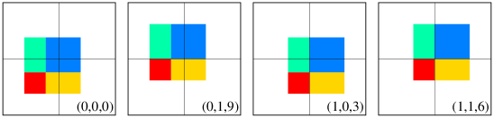
Figure 2. Four square windows corresponding to different DP tilings. The underlying inflation rules form a single orbit under the action of the group $D_{4}$, and the resulting tilings belong to one MLD class, because the corresponding tilings simply are translates of one another, hence related by a local derivation rule.

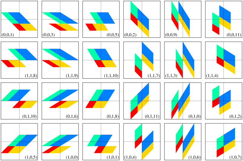
Figure 3. Further 24 polygonal windows corresponding to different DPV tilings. One can recognise 3 orbits of inflation rules under the action of the group $D_{4}$, namely those of the elements $(0,0,1)$ (first and fourth column), $(0,0,3)$ (second and fifth column) and $(0,0,5)$ (third and sixth column). Moreover, the 12 obvious pairs of windows (with equal slope) representing 12 different MLD classes can be recognised.

The polygonal windows can be further divided into two main classes. One, with the square windows, corresponds to the four possible direct product tilings (Figure 2) and lie in the same LI class [1]. The remaining class with 24 cases, as depicted in Figure 3, can be further understood as three orbits under the action of the dihedral group $D_{4}$. This action is clearly recognisable at the level of inflation rules, but becomes less obvious at the level of windows. One would expect that the action of the group $D_{4}$ in the direct space will have its counterpart in the internal space – a parallelogram is mapped to another parallelogram under the action. This is not true, as can be seen by comparing cases $(0,0,1)$ and $(1,1,8)$. These tilings are related by a rotation through $\pi$ while the windows need some additional rearrangement. The origin for this is our choice of the control points in each tile, which is not invariant under the action of $D_{4}$. While the point set obtained from the tiling $(0,0,1)$ via a rotation through $\pi$ is not the one given by the control points of tiling $(1,1,8)$, it is MLD with this point set. This can be undone by applying a local rule (changing the control points in each type of tile). These local rules consist of a set of translations $t_{i}\in\mathbb{Z}[\tau]^{2}$ of $\varLambda_{i}$, which result in a set of translation $t^{\star}_{i}\in\mathbb{Z}[\tau]^{2}$ of $\varOmega_{i}$ in the internal space.

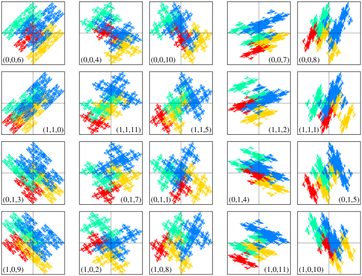
Figure 4. The 20 fractal windows corresponding to different DPV tilings. The first column – “castle” – corresponds to an orbit of rule $(0,0,6)$ under the action of $D_{4}$. Since the inflation rule has a mirror symmetry, the resulting orbit consist of four elements. The second and third column display an orbit of rule $(0,0,4)$ – “cross”. The last two columns correspond to the orbit of rule $(0,0,7)$ – type “island”.

Based on the general MLD criterion, see [2, Rem. 7.6] or [5], one can further divide the 24 tilings with sheared parallelogram windows into 12 MLD classes. Two tilings in each class are related by a rotation through $\pi$, which is a product of two reflections, namely across coordinate axes. As mentioned above, the corresponding windows are also related by this rotation (after a change of the control points). This shows that the two tilings in each MLD class are elements of the same tiling hull. This hull then possesses rotational symmetry.

Since there are six different shearing angles $\varphi$, namely

$$\varphi\in\left\{\pm\frac{\raisebox{-2.0pt}{$\pi$}}{\raisebox{0.5pt}{$4$}},\,\pm\arctan(\tau),\,\pm\arctan\left(\tau^{-1}\right)\right\},$$ (4.1)

in two possible directions (along the $x$-axis, and the $y$-axis respectively), the MLD classification based on the slope of the windows is clear.

5. Relations via topological conjugacy

Two tilings that are MLD clearly define two dynamical systems that are topologically conjugate. The converse, however, is not true in general because we are not in a symbolic setting. In particular, there is no analogue of the Curtis–Hedlund–Lyndon theorem. In fact, local derivability is the concept replacing it, but now only representing one possibility of topological conjugacy. Therefore, some DPV tilings that are not MLD could still give topologically conjugate dynamical systems. This is indeed the case, as we first demonstrate with an example.

Let us focus on the tiling with rule $(0,0,1)$. We will show that the dynamical system defined by this tiling is topologically conjugate with a DP tiling. This result should not be surprising. It follows from the general MLD criterion that two tilings are MLD if and only if one can obtain one window from the other by using just a finite number of Boolean operations (intersection, union, complement) and translations by elements from $\pi_{\!{}_{\perp}}(\mathcal{L})=\mathbb{Z}[\tau]^{2}$. Having a DP tiling (with a square window), one can use it to approximate tiling $(0,0,1)$ with increasing precision. The general MLD criterion ensures that all the approximating tilings are MLD. If the vertices of the sheared window belong to $\pi_{\!{}_{\perp}}(\mathcal{L})=\mathbb{Z}[\tau]^{2}$, the consideration above suggests that the tiling with the sheared window may no longer be MLD with the DP tiling, but remains topologically conjugate to it; see Figure 5 for an illustration.

Figure 5. Approximation of a parallelogram using a square and finitely many Boolean operations. This suggests topological conjugacy under some additional constraints on the vertex points of the parallelogram.

If two tilings are MLD, there exists a set of local derivation rules in both directions (meaning that, from the knowledge of one tiling on a uniformly bounded neighbourhood of any point, one can construct the other tiling at this point). As approximants approach the tiling with the sheared window, the diameter of the required neighbourhood grows without bound and, in the limit, one needs to know the whole tiling in order to construct the sheared tiling at any given place. Thus the locality is broken. On the other hand, it is natural to ask whether there is some weaker relation between the tiling with sheared window and the DP tiling. The answer is affirmative, and the relation is topological conjugacy, as we demonstrate next.

For the tiling with rule $(0,0,1)$, one can use a different inflation rule (which is no longer a stone inflation) that defines the same tiling. This (crucial) step relies on the fact that the original tiling has a striped structure, where each “row” is nothing but a 1D Fibonacci tiling. Following the standard procedure described for example in [8], or by solving the following iterated IFS, respectively the adjoint IFS to the modified rule, one obtains a set of new prototiles $P_{i}$ that satisfy

$$\begin{split}P_{0}&\,=\,\tau^{-1}P_{3}\hskip 0.5pt,\\ P_{1}&\,=\,\tau^{-1}P_{2}+\bigl{(}\begin{smallmatrix}1\\ 0\end{smallmatrix}\bigr{)}\,\cup\,\tau^{-1}P_{3}\hskip 0.5pt,\\ P_{2}&\,=\,\tau^{-1}P_{1}+\bigl{(}\begin{smallmatrix}-1\\ 1\end{smallmatrix}\bigr{)}\,\cup\,\tau^{-1}P_{3}\hskip 0.5pt,\\ P_{3}&\,=\,\tau^{-1}P_{0}+\bigl{(}\begin{smallmatrix}0\\ 1\end{smallmatrix}\bigr{)}\,\cup\,\tau^{-1}P_{1}+\bigl{(}\begin{smallmatrix}-1\\ 1\end{smallmatrix}\bigr{)}\,\cup\,\tau^{-1}P_{2}+\bigl{(}\begin{smallmatrix}1\\ 0\end{smallmatrix}\bigr{)}\,\cup\,\tau^{-1}P_{3}\hskip 0.5pt.\end{split}$$ (5.1)

They turn the rearrangement of rule $(0,0,1)$ into a stone inflation that is MLD with the rearranged $(0,0,1)$ rule, and thus with the $(0,0,1)$ tiling itself; see Figure 6 for an illustration. Note that the new tiles $P_{i}$ are related to the original tiles $T_{i}$ by the shearing matrix $S=\left(\begin{smallmatrix}1&-1\\ 0&1\end{smallmatrix}\right)$. For obvious reasons, we call this tiling a sheared DP tiling. So, the $(0,0,1)$ rearrangement is MLD with a sheared $(0,0,0)$ tiling, but not with $(0,0,0)$ itself. However, $(0,0,1)$ and $(0,0,0)$ can give rise to topologically conjugate systems, as we show below.

Figure 6. The stone inflation rule $(0,0,1)$ and the rule in the middle produce the same tiling. The rearranged rule $(0,0,1)$ and the sheared $(0,0,0)$ rule define two tilings that are MLD. We show that the sheared $(0,0,0)$ tiling and the DP tiling $(0,0,0)$ are topologically conjugate and thus prove the topological conjugacy between the tiling spaces for $(0,0,0)$ and $(0,0,1)$.

If one denotes by $\varLambda_{\bullet}$ the chosen fixed point of the DP tiling $(0,0,0)$ and by $\varSigma_{\bullet}$ the matching fixed point of the sheared tiling, there is a clear correspondence via $\varSigma_{\bullet}=S\varLambda_{\bullet}$. The procedure described above can be applied to all 24 tilings with the polygonal window from Figure 3.

Fact 5.1.

In the case of Fibonacci DPVs, each tiling with a polygonal window as in Figure 3 is MLD to a sheared DP tiling with a shearing matrix $S$ of the form

$$\begin{pmatrix}1&\alpha\\ 0&1\end{pmatrix}\ \mbox{or}\ \begin{pmatrix}1&0\\ \alpha&1\end{pmatrix},\quad\mbox{each with }\alpha\in\left\{\pm 1,\ \pm\tau,\ \pm\tau^{-1}\right\},$$ (5.2)

which corresponds to the angles from Eq. (4.1). ∎

The shearing map $S$ acting in direct space has its counterpart in internal space, which we call $S^{\star}$. The entries of this matrix are the images of the corresponding entries of $S$ under the field automorphism ^′. Since $\tau$ is a unit in $\mathbb{Z}[\tau]$, the following observations hold.

Fact 5.2.

For the lattice $\mathcal{L}$, one has $\left(S\oplus S^{\star}\right)\mathcal{L}=\mathcal{L}$. Consequently, $S\varLambda_{\bullet}$ is a regular model set for the lattice $\mathcal{L}$, with a subset of $S^{\star}\varOmega$ of full measure as its window. ∎

Note that the window in this statement contains the entire interior of $S^{\star}\varOmega$, but only part of its boundary. Since $S$ is an invertible linear mapping, we also get the following result.

Fact 5.3.

The mapping $S$ is a bijection on $\mathbb{R}\hskip 0.5pt^{2}$, and $S^{\star}$ is a bijection on $L^{\star}$. In particular, if $\varSigma=S\varLambda$, then $0\in\varLambda$ if and only if $0\in\varSigma$. Moreover, $\varLambda$ is a generic model set if and only if $\varSigma$ is a generic model set, i.e., $\partial\varOmega\cap L^{\star}=\varnothing$ if and only if $\partial(S^{\star}\varOmega)\cap L^{\star}=\varnothing$. ∎

In order to proceed, one has to define dynamical systems induced by the tilings $\varLambda_{\bullet}$ and $\varSigma_{\bullet}$. As usual, one defines the geometric hulls

$$\mathbb{X}\,=\,\overline{\big{\{}\varLambda_{\bullet}+t:t\in\mathbb{R}\hskip 0.5pt^{2}\big{\}}}^{\mathrm{LT}}\quad\mbox{and}\quad\mathbb{Y}\,=\,\overline{\big{\{}\varSigma_{\bullet}+t:t\in\mathbb{R}\hskip 0.5pt^{2}\big{\}}}^{\mathrm{LT}},$$ (5.3)

where the closure is taken in the local topology, which is metrisable [11]. In such a metric $\hskip 0.5pt\mathrm{d}$, two tilings are close if they agree on a large ball centred at the origin, possibly after a small global translation of one of them. Formally, two tilings $\varLambda$ and $\widetilde{\varLambda}$ are $\varepsilon$-close, $\hskip 0.5pt\mathrm{d}(\varLambda,\widetilde{\varLambda})<\varepsilon$, if

$$\varLambda\,\cap\,\overline{B_{\nicefrac{{1}}{{\varepsilon}}}(0)}\,=\,(\widetilde{\varLambda}+t)\,\cap\,\overline{B_{\nicefrac{{1}}{{\varepsilon}}}(0)}\quad\mbox{for some }t\in B_{\varepsilon}(0)\hskip 0.5pt.$$

Note that the metric $\hskip 0.5pt\mathrm{d}$ is not translation invariant.

Both hulls are equipped with the action of $\mathbb{R}\hskip 0.5pt^{2}$ via translation. This turns $\mathbb{X}$ and $\mathbb{Y}$ into a pair of topological dynamical systems, $(\mathbb{X},\mathbb{R}\hskip 0.5pt^{2})$ and $(\mathbb{Y},\mathbb{R}\hskip 0.5pt^{2})$. Since the defining inflation rules are both primitive, the resulting tilings are repetitive which is equivalent to the statement that the dynamical hulls $\mathbb{X}$ and $\mathbb{Y}$ are minimal. Our aim is to prove that these dynamical systems are topologically conjugate, which is to say that there exists a homeomorphism $\phi\colon\mathbb{X}\longrightarrow\mathbb{Y}$ which preserves the action $g_{t}$ of the group $\mathbb{R}\hskip 0.5pt^{2}$ via translation. Then, $\phi$ is a topological conjugacy (in the strict sense) if $g_{t}\circ\phi=\phi\circ g_{t}$ holds for all $t\in\mathbb{R}\hskip 0.5pt^{2}$. In other words, the diagram

$$\begin{CD}\mathbb{X}@>{g_{t}}>{}>\mathbb{X}\\ @V{\phi}V{}V@V{}V{\phi}V\\ \mathbb{Y}@>{g_{t}}>{}>\mathbb{Y}\end{CD}$$ (5.4)

is commutative.

The strategy from here goes as follows. It is not difficult to see that all patterns with polygonal windows are MLD with a sheared DP tiling. In a first step, in each row (or column) of the tiling, all tiles are replaced by equally sheared versions, and one then observes that this tiling with sheared tiles is actually MLD to a sheared DP tiling, which in turn is combinatorially equivalent to the plain DP tiling. It is important here that the applied shear preserves the projected lattice $\pi(\mathcal{L})$, and thus lifts to an automorphism of $\mathcal{L}$. While this shear of the DP tiling is not an MLD operation, it is still a topological conjugacy of the underlying dynamical system. To show this, we select a suitable pair of tilings and construct a bijection between the respective translation orbits that commutes with the translation action. Then, invoking the common parametrisation from the projection method, we show via a somewhat subtle limit argument that this bijection between the two orbits extends to a homeomorphism of the hulls with the same properties.

To proceed, we need to recall several results. First, since $\varLambda_{\bullet}$ is a regular model set that arises from the cut and project scheme $(\mathbb{R}\hskip 0.5pt^{2},\,\mathbb{R}\hskip 0.5pt^{2},\,\mathcal{L})$ with $\mathcal{L}$ defined in (3.5), there exists an $\mathbb{R}\hskip 0.5pt^{2}$-invariant surjective continuous mapping $\beta_{\mathbb{X}}$, called the torus parametrisation, which maps the hull $\mathbb{X}$ onto the torus $\mathbb{T}(\varLambda_{\bullet})$. This torus is defined for our set $\varLambda_{\bullet}$ as a factor group, $\mathbb{T}(\varLambda_{\bullet})\mathrel{\mathop{:}}=(\mathbb{R}\hskip 0.5pt^{2}\times\mathbb{R}\hskip 0.5pt^{2})/\mathcal{L}$. The mapping $\beta_{\mathbb{X}}$ is, under our assumptions, 1–1 almost everywhere, but not everywhere; see [9, Cor. 5.2] or [4] for a detailed exposition.

As already mentioned above, the cut and project scheme for set $\varSigma_{\bullet}$ is exactly the same as the one for the set $\varLambda_{\bullet}$. Therefore, we can employ the same torus. This fact is useful for our further discussion. We provide this connection by choosing an appropriate torus parametrisation for the two hulls. In particular, both tilings $\varLambda_{\bullet}$ and $\varSigma_{\bullet}$ are mapped to $0$. Note that, since $\varLambda_{\bullet}$ is a singular element of $\mathbb{X}$, we have

$$\varLambda_{\bullet}\,\subsetneq\,\mbox{\Large$\curlywedge$}(\varOmega)\,=\,\{x\in\mathbb{Z}[\tau]^{2}\ :x^{\star}\in\varOmega\}.$$

From the minimality of the hulls $\mathbb{X}$ and $\mathbb{Y}$ and from the choice of the torus parametrisation, it follows that one can now choose generic elements

$$\varLambda_{\circ}\in\mathbb{X}\quad\mbox{and}\quad\varSigma_{\circ}\in\mathbb{Y}$$ (5.5)

such that they are mapped to the same point on the torus,

$$\beta_{\mathbb{X}}(\varLambda_{\circ})\,=\,\beta_{\mathbb{Y}}(\varSigma_{\circ})\,=\,\vartheta\,\neq\,0\hskip 0.5pt.$$

The point $\vartheta\in\mathbb{R}\hskip 0.5pt^{4}$ is fixed and chosen so that $\varLambda_{\circ}=\mbox{\Large$\curlywedge$}(\varOmega_{\vartheta})$, with $\varOmega_{\vartheta}\mathrel{\mathop{:}}=\varOmega+\pi_{\!{}_{\perp}}\!(\vartheta)$. Moreover, the minimality implies that $\mathbb{X}=\overline{\varLambda_{\circ}+\mathbb{R}\hskip 0.5pt^{2}\hskip 0.5pt}^{\mathrm{LT}}$ and $\mathbb{Y}=\overline{\varSigma_{\circ}+\mathbb{R}\hskip 0.5pt^{2}\hskip 0.5pt}^{\mathrm{LT}}$.

Now, we are in the position to construct the homeomorphism $\phi$ explicitly and show that it has the properties of a topological conjugacy. The first step consists in defining the orbit mapping

$$\phi\colon\{\varLambda_{\circ}+t:t\in\mathbb{R}\hskip 0.5pt^{2}\}\,\longrightarrow\,\{\varSigma_{\circ}+t:t\in\mathbb{R}\hskip 0.5pt^{2}\}$$

as follows:

1. $\phi(\varLambda_{\circ})=\varSigma_{\circ}$,

2. $\phi(\varLambda_{\circ}+t)=\varSigma_{\circ}+t$ for every $t\in\mathbb{R}\hskip 0.5pt^{2}$.

It is clear by construction that $\phi$ is invertible on this orbit, and that it satisfies the required commutation property,

$$\bigl{(}g_{t}\circ\phi\bigr{)}(\varLambda_{\circ}+T)\,=\,g_{t}(\varSigma_{\circ}+T)\,=\,\varSigma_{\circ}+T+t\,=\,\phi(\varLambda_{\circ}+T)+t\,=\,\bigl{(}\phi\circ g_{t}\bigr{)}(\varLambda_{\circ}+T)\hskip 0.5pt.$$ (5.6)

Our torus parametrisations ensures that $\beta_{\mathbb{Y}}(\phi(\varLambda_{\circ}+t))=\beta_{\mathbb{X}}(\varLambda_{\circ}+t)$, i.e., the orbit of an element $\varLambda_{\circ}\in\mathbb{X}$ has the same image on the torus as the orbit of $\phi(\varLambda_{\circ})$ in the hull $\mathbb{Y}$.

To establish that $\phi$ has an extension to a continuous bijection between $\mathbb{X}$ and $\mathbb{Y}$ is more subtle. Let us first state two results that hold for an arbitrary, generic model set $\varLambda$.

Lemma 5.4.

Let $\varLambda$ be a regular model set, with window $\varOmega_{\!\varLambda}$. Assume $\varLambda$ to be generic, so $\partial\varOmega_{\!\varLambda}\cap\varLambda^{\star}=\varnothing$. Let $\varLambda_{R}=\varLambda\cap\overline{B_{R}(0)}$. Then, for all $R>0$, there exists some $\delta=\delta(R)$ such that, for all $t^{\star}\in\mathbb{R}\hskip 0.5pt^{2}$ with $\|t^{\star}\|<\delta$, one has

$$\varLambda_{R}^{\star}\,\subset\,\varOmega_{\!\varLambda}\cap(\varOmega_{\!\varLambda}+t^{\star})\hskip 0.5pt.$$

In particular, the claim holds for $\varLambda=\varLambda_{\circ}$.

Proof.

Fix $R>0$. Since $\varLambda$ is uniformly discrete and hence locally finite, it follows that $\varLambda_{R}$ is finite, so $\varLambda_{R}^{\star}$ is finite as well. This assumption assures that

$$\delta\,\mathrel{\mathop{:}}=\min_{x^{\star}\in\varLambda_{R}^{\star}}\operatorname{dist}(x^{\star}\!,\partial\varOmega_{\!\varLambda})$$

is well defined. The assumption on regularity of the set $\varLambda$ results in $\delta>0$. Then, for all $x^{\star}\in\varLambda_{R}^{\star}$, one gets $x^{\star}\in\varOmega_{\!\varLambda}+t^{\star}$, and we are done. ∎

Remark 5.5.

Requiring genericity of $\varLambda$ can often be relaxed by replacing it with several constraints on the direction of the vector $t^{\star}$. In our case at hand, this can easily be done since the shape of the window $\varOmega$ is a polygon and thus sufficiently simple. $\Diamond$

One immediate consequence of Lemma 5.4 is the following result.

Proposition 5.6.

Let $\varLambda$ be a regular model set that is generic, so $\varLambda^{\star}\,\cap\,\partial\varOmega_{\!\varLambda}=\varnothing$. Further, let $t\in L=\mathbb{Z}[\tau]^{2}$. Then, there are $\delta_{1}=\delta_{1}(\varepsilon)>0$ and $\delta_{2}=\delta_{2}(\varepsilon)>0$ such that, if $\varLambda$ and $\varLambda+t$ are $\varepsilon$-close, then $\|t^{\star}\|<\delta_{1}$, and, if $\|t^{\star}\|<\delta_{2}$, then $\varLambda$ and $\varLambda+t$ are $\varepsilon$-close.

Proof.

Denote by $A_{\varepsilon}$ the set of $\varepsilon$-almost periods of $\varLambda$ relative to $\hskip 0.5pt\mathrm{d}$, so

$$A_{\varepsilon}\,=\,\{t:\hskip 0.5pt\mathrm{d}(\varLambda,\varLambda+t)<\varepsilon\}\hskip 0.5pt.$$

Then, the statements hold if there exist $\delta_{1}$ and $\delta_{2}$ such that

$$B_{\delta_{2}}(0)\,\subseteq\,\overline{A_{\varepsilon}^{\star}}\,\subseteq\,B_{\delta_{1}}(0)\hskip 0.5pt.$$

Clearly, $\delta_{2}$ can be chosen as described in Lemma 5.4. The second bound can be obtained as $\delta_{1}\mathrel{\mathop{:}}=\sup\{\,\|t\|\,:\,t\in\mathbb{R}\hskip 0.5pt^{2},\,t+\varLambda^{\star}_{1/\varepsilon}\subset\varOmega_{\!\varLambda}\}$. ∎

Proposition 5.6 can directly be applied to our situation. Suppose that $\varLambda_{\circ}$ and $\varLambda_{\circ}+t$ are $\varepsilon$-close, so $\hskip 0.5pt\mathrm{d}(\varLambda_{\circ},\,\varLambda_{\circ}+t)<\varepsilon$. This implies that $\|t^{\star}\|<\delta(\varepsilon)$. Then, for $S=\left(\begin{smallmatrix}1&\alpha\\ 0&1\end{smallmatrix}\right)$, we get

$$\big{\|}(S^{-1}t)^{\star}\big{\|}\,=\,\big{\|}t^{\star}-\alpha^{\star}\bigl{(}\begin{smallmatrix}t^{\star}_{1}\\ 0\end{smallmatrix}\bigr{)}\big{\|}\,\leqslant\,\bigl{(}1+|\alpha^{\star}|\bigr{)}\|t^{\star}\|\,\leqslant\,\bigl{(}1+|\alpha^{\star}|\bigr{)}\delta(\varepsilon)\hskip 0.5pt.$$

Note that the same estimate holds also for any matrix $S$ of the form $S=\left(\begin{smallmatrix}1&0\\ \alpha&1\end{smallmatrix}\right)$.

Proposition 5.6 ensures that there is some $\widetilde{\varepsilon}\in\mathcal{O}(\varepsilon)$ such that $\varLambda_{\circ}$ and $\varLambda_{\circ}+S^{-1}t$ are $\widetilde{\varepsilon}$-close which here is equivalent to the statement that $\varLambda_{\circ}$ and $\varLambda_{\circ}+S^{-1}t$ agree on $\overline{B_{\nicefrac{{1}}{{\widetilde{\varepsilon}}}}(0)}$. Applying $S$ yields that $S\varLambda_{\circ}$ and $S\varLambda_{\circ}+SS^{-1}t=S\varLambda_{\circ}+t$ agree on $S\overline{B_{\nicefrac{{1}}{{\widetilde{\varepsilon}}}}(0)}$. Since the matrix $S$ is invertible, $S\overline{B_{\nicefrac{{1}}{{\widetilde{\varepsilon}}}}(0)}$ is an ellipse centred at the origin. Therefore, there exists $R>0$ such that $B_{R}(0)\subset S\overline{B_{\nicefrac{{1}}{{\widetilde{\varepsilon}}}}(0)}$, where the radius $R$ actually satisfies

$$R\,<\,\frac{\raisebox{-2.0pt}{$c$}}{\raisebox{0.5pt}{$\widetilde{\varepsilon}$}}\quad\mbox{with}\quad c\,=\,\frac{\raisebox{-2.0pt}{$1$}}{\raisebox{0.5pt}{$\sqrt{2}$}}\sqrt{\alpha^{2}-\alpha\sqrt{\alpha^{2}+4\hskip 0.5pt}+2\hskip 0.5pt}.$$

Note that $c$ is the smaller singular value of $S$. Taking $\underline{\varepsilon}$ such that $R\geqslant\frac{1}{\underline{\varepsilon}}$ results in the following claim.

Proposition 5.7.

Let $\varLambda_{\circ}$ be the regular, generic model set from (5.5), so $\varLambda^{\star}_{\circ}\,\cap\,\partial\varOmega_{\vartheta}=\varnothing$. Further, let $t\in\mathbb{Z}[\tau]^{2}$. Then, if $\varLambda_{\circ}$ and $\varLambda_{\circ}+t$ are $\varepsilon$-close, $\varSigma_{\circ}$ and $\varSigma_{\circ}+t$ are $\underline{\varepsilon}$-close, with $\underline{\varepsilon}\in\mathcal{O}(\varepsilon)$. Formally, $\hskip 0.5pt\mathrm{d}(\varLambda_{\circ},\,\varLambda_{\circ}+t)<\varepsilon\ \Rightarrow\ \hskip 0.5pt\mathrm{d}(\varSigma_{\circ},\,\varSigma_{\circ}+t)<\underline{\varepsilon}\hskip 0.5pt.$ ∎

Remark 5.8.

Since the set $\varLambda$ is aperiodic, the set of its periods is trivial, so

$$\varLambda+t\,=\,\varLambda\quad\Longleftrightarrow\quad t\,=\,0\hskip 0.5pt,$$

and the following implication holds for $(t_{n})_{n\in\mathbb{N}}$ with $t_{n}\in\mathbb{Z}[\tau]^{2}$,

$$\lim_{n\to\infty}\varLambda+t_{n}=\varLambda\quad\Longrightarrow\quad\lim_{n\to\infty}t^{\star}_{n}=0\hskip 0.5pt.$$ (5.7)

This has an immediate consequence, namely $(t_{n})_{n\in\mathbb{N}}$ is eventually 0, or $t_{n}$ has a subsequence that grows unboundedly. Therefore, if

$$\lim_{n\to\infty}\varLambda+t_{n}\,=\lim_{n\to\infty}\varLambda+s_{n}\quad\mbox{for }t_{n},s_{n}\in\mathbb{Z}[\tau]^{2},$$

then $(t_{n}-s_{n})_{n\in\mathbb{N}}$ is eventually 0, or unboundedly growing such that $\lim_{n\to\infty}(t_{n}-s_{n})^{\star}=0$. Note that the converse of (5.7) is not true due to the existence of singular elements in the hull $\mathbb{X}$. Such elements always exist when $\varLambda$ is aperiodic [4]. $\Diamond$

Proposition 5.7 is a good starting point for our proof of the continuity of $\phi$, as $\varSigma_{\circ}=\phi(\varLambda_{\circ})$ and $\varSigma_{\circ}+t=\phi(\varLambda_{\circ}+t)$. Since the distance $\hskip 0.5pt\mathrm{d}$ is not translation invariant, one has to work with converging sequences. Thus, our next aim is to show that, if $\varLambda_{\circ}+t_{n}$ approaches $\varLambda_{\circ}$ in $\mathbb{X}$, then $\phi(\varLambda_{\circ}+t_{n})$ approaches $\phi(\varLambda_{\circ})$ in $\mathbb{Y}$.

Lemma 5.9.

Let $\varLambda_{\circ}$ be the regular, generic model set from (5.5). If $\varLambda_{\circ}+t_{n}$ approximates $\varLambda_{\circ}$ in $\mathbb{X}$ with $t_{n}\in\mathbb{R}\hskip 0.5pt^{2}$, then $\phi(\varLambda_{\circ}+t_{n})$ approximates $\phi(\varLambda_{\circ})$ in $\mathbb{Y}$, formally

$$\lim_{n\to\infty}\hskip 0.5pt\mathrm{d}(\varLambda_{\circ},\varLambda_{\circ}+t_{n})=0\,\Longrightarrow\lim_{n\to\infty}\hskip 0.5pt\mathrm{d}\bigl{(}\phi(\varLambda_{\circ}),\phi(\varLambda_{\circ}+t_{n})\bigr{)}=0\hskip 0.5pt.$$

Proof.

We distinguish between two cases. First, let us assume that the sequence $(t_{n})_{n\in\mathbb{N}}$ consists of elements of $\mathbb{Z}[\tau]^{2}$ only. Then, the claim holds due to Proposition 5.7.

Thus, suppose that the $t_{n}$ lie in $\mathbb{R}\hskip 0.5pt^{2}$. Since $\mathbb{Z}[\tau]^{2}$ is dense in $\mathbb{R}\hskip 0.5pt^{2}$, there exists a sequence $(\delta_{n})_{n\in\mathbb{N}}$ with $\delta_{n}\in\mathbb{R}\hskip 0.5pt^{2}$ such that $t_{n}+\delta_{n}\in\mathbb{Z}[\tau]^{2}$ and $\|\delta_{n}\|<\frac{1}{2^{n}}$ for all $n\in\mathbb{N}$ . Since $\varLambda_{\circ}+t_{n}$ and $\varLambda_{\circ}+t_{n}+\delta_{n}$ agree on the whole plane up to a translation by $\delta_{n}$, they are $\frac{1}{2^{n}}$-close. Using the triangle inequality, one obtains

$$\hskip 0.5pt\mathrm{d}(\varLambda_{\circ},\varLambda_{\circ}+t_{n}+\delta_{n})\,\leqslant\,\hskip 0.5pt\mathrm{d}(\varLambda_{\circ},\varLambda_{\circ}+t_{n})+\hskip 0.5pt\mathrm{d}(\varLambda_{\circ}+t_{n},\varLambda_{\circ}+t_{n}+\delta_{n})\,<\,\hskip 0.5pt\mathrm{d}(\varLambda_{\circ},\varLambda_{\circ}+t_{n})+\frac{\raisebox{-2.0pt}{$1$}}{\raisebox{0.5pt}{$2^{n}$}}\hskip 0.5pt.$$

Therefore, $\hskip 0.5pt\mathrm{d}(\varLambda_{\circ},\varLambda_{\circ}+t_{n}+\delta_{n})\xrightarrow{n\to\infty}0$, and we can use the first part of this claim since $t_{n}+\delta_{n}\in\mathbb{Z}[\tau]^{2}$. Thus,

$$\lim_{n\to+\infty}\hskip 0.5pt\mathrm{d}\bigl{(}\phi(\varLambda_{\circ}),\phi(\varLambda_{\circ}+t_{n}+\delta_{n})\bigr{)}\,=\,0\hskip 0.5pt.$$

From the fact that $\varLambda_{\circ}+t_{n}$ and $\varLambda_{\circ}+t_{n}+\delta_{n}$ are $\frac{1}{2^{n}}$-close, it follows (by construction) that also $\phi(\varLambda_{\circ}+t_{n})$ and $\phi(\varLambda_{\circ}+t_{n}+\delta_{n})=\phi(\varLambda_{\circ}+t_{n})+\delta_{n}$ are $\frac{1}{2^{n}}$-close. Thus, using the triangle inequality again, one concludes that

$$\hskip 0.5pt\mathrm{d}\bigl{(}\phi(\varLambda_{\circ}),\phi(\varLambda_{\circ}+t_{n})\bigr{)}\,\leqslant\,\hskip 0.5pt\mathrm{d}\bigl{(}\phi(\varLambda_{\circ}),\phi(\varLambda_{\circ}+t_{n}+\delta_{n})\bigr{)}+\frac{\raisebox{-2.0pt}{$1$}}{\raisebox{0.5pt}{$2^{n}$}}\,\xrightarrow{n\to\infty}\,0\hskip 0.5pt,$$

which proves our claim. ∎

Lemma 5.10.

Let $T\in\mathbb{R}\hskip 0.5pt^{2}$. Then, for the regular, generic model set $\varLambda_{\circ}$ from (5.5), one has

$$\lim_{n\to\infty}\hskip 0.5pt\mathrm{d}(\varLambda_{\circ}+T,\varLambda_{\circ}+t_{n})=0\,\Longrightarrow\lim_{n\to\infty}\hskip 0.5pt\mathrm{d}\bigl{(}\phi(\varLambda_{\circ}+T),\phi(\varLambda_{\circ}+t_{n})\bigr{)}\,=\,0\hskip 0.5pt.$$

Proof.

Suppose that $\lim_{n\to\infty}\hskip 0.5pt\mathrm{d}(\varLambda_{\circ}+T,\,\varLambda_{\circ}+t_{n})=0$. Then, $\varLambda_{\circ}+T$ and $\varLambda_{\circ}+t_{n}$ are $\varepsilon_{n}$-close which means that they coincide on a ball $\overline{B_{\nicefrac{{1}}{{\varepsilon_{n}}}}(0)}$ up to a small translation. This is equivalent to the statement that $\varLambda_{\circ}$ and $\varLambda_{\circ}+t_{n}-T$ agree on a ball $\overline{B_{\nicefrac{{1}}{{\varepsilon_{n}}}}(T)}$. From the assumption, one has $\varepsilon_{n}\to 0$ as $n\to\infty$ and thus there exists $n_{0}$ with $0\in\overline{B_{\nicefrac{{1}}{{\varepsilon_{n}}}}(T)}$ for all $n\geqslant n_{0}$. Then, $B_{\nicefrac{{1}}{{\varepsilon^{\prime}_{n}}}}(0)\subset\overline{B_{\nicefrac{{1}}{{\varepsilon_{n}}}}(T)}$ with $\frac{1}{\varepsilon^{\prime}_{n}}=\frac{1}{\varepsilon_{n}}-\|T\|$. Hence $\varepsilon^{\prime}_{n}=\frac{1}{\nicefrac{{1}}{{\varepsilon_{n}}}-\|T\|}$, which shows that $\varepsilon^{\prime}_{n}\to 0$ as $n\to\infty$. Lemma 5.9 now implies the claim. ∎

At this point, one has to extend the mapping $\phi$ to the closure of the orbit of $\varLambda_{\circ}$, i.e., to the hull $\mathbb{X}$. Note that this step profits from the minimality of $\mathbb{X}$ and from the fact that we may use the same torus for $\mathbb{X}$ and $\mathbb{Y}$. Recall that $\partial\varOmega_{\vartheta}\cap L^{\star}=\varnothing$ if and only if $\partial(S^{\star}\varOmega_{\vartheta})\cap S^{\star}L^{\star}=\partial(S^{\star}\varOmega_{\vartheta})\cap L^{\star}=\varnothing$. This allows us to identify the fibres corresponding to singular points in each hull. Thus, if a sequence $(\varLambda_{\circ}+t_{n})_{n\in\mathbb{N}}$ converges towards a singular element $\widetilde{\varLambda}\in\mathbb{X}$, our choice ensures that, if $(\varSigma_{\circ}+t_{n})_{n\in\mathbb{N}}$ converges in $\mathbb{Y}$, the resulting limit point $\widetilde{\varSigma}$ is also singular. This would allow us to continuously extend the mapping $\phi$ to the hull $\mathbb{X}$ by defining $\phi(\widetilde{\varLambda})\mathrel{\mathop{:}}=\lim_{n\to\infty}\varSigma_{\circ}+t_{n}=\widetilde{\varSigma}$.

The following lemma shows that the above consideration about the convergence holds.

Lemma 5.11.

Let $\varLambda_{\circ}$ be the regular, generic model set from (5.5). Suppose that we have $\varLambda_{\circ}+t_{n}\xrightarrow{n\to\infty}\widetilde{\varLambda}$ with $\widetilde{\varLambda}\in\mathbb{X}$. Then, the sequence $(\varSigma_{\circ}+t_{n})_{n\in\mathbb{N}}$ converges in $\mathbb{Y}$.

Proof.

If $\varLambda_{\circ}+t_{n}$ converges towards a generic element $\widetilde{\varLambda}$, then $\beta_{\mathbb{X}}(\varLambda_{\circ}+t_{n})\xrightarrow{n\to\infty}\beta_{\mathbb{X}}(\widetilde{\varLambda})$. Since $\beta_{\mathbb{X}}(\varLambda_{\circ}+t_{n})=\beta_{\mathbb{Y}}(\varSigma_{\circ}+t_{n})$ and $\beta^{-1}_{\mathbb{Y}}\bigl{(}\{\beta_{\mathbb{X}}(\widetilde{\varLambda})\}\bigr{)}$ contains only one element, the claim follows immediately.

Now, suppose that the limit point $\widetilde{\varLambda}$ of $\varLambda_{\circ}+t_{n}$ is a singular element of $\mathbb{X}$. We show the claim by a contradiction. For this purpose suppose that $\lim_{n\to\infty}\varSigma_{\circ}+t_{n}$ does not exist, i.e., the sequence $(\varSigma_{\circ}+t_{n})_{n\in\mathbb{N}}$ has at least two accumulation points. Without loss of generality, one may assume that $(\varSigma_{\circ}+t_{n})_{n\in\mathbb{N}}$ has exactly two accumulation points, say $\varSigma_{1}$ and $\varSigma_{2}$ with $\varSigma_{1}\neq\varSigma_{2}$. Then, there exist two subsequences of $(t_{n})_{n\in\mathbb{N}}$, say $(s_{n})_{n\in\mathbb{N}}=(t_{k_{n}})_{n\in\mathbb{N}}$ and $(r_{n})_{n\in\mathbb{N}}=(t_{\ell_{n}})_{n\in\mathbb{N}}$ with $\varSigma_{1}=\lim_{n\to\infty}\varSigma_{\circ}+s_{n}$, and $\varSigma_{2}=\lim_{n\to\infty}\varSigma_{\circ}+r_{n}$, respectively. These subsequences can be chosen so that $\{s_{n}\,:\,n\in\mathbb{N}\}\cap\{r_{n}\,:\,n\in\mathbb{N}\}=\varnothing$.

Since the limit points are not equal, there exists a position where they differ. This allows us to find a ball centred at the origin on which $\varSigma_{1}$ and $\varSigma_{2}$ do not coincide. Thus, there is an index $n_{0}$ with

$$\bigl{(}(\varSigma_{\circ}+s_{n_{0}})\triangle(\varSigma_{\circ}+r_{n_{0}})\bigr{)}\cap B_{n_{0}}(0)\,\neq\,\varnothing$$ (5.8)

with $\triangle$ standing for the symmetric difference of two sets. Set $N\mathrel{\mathop{:}}=\max\,\{k_{n_{0}},\ell_{n_{0}}\}$ and define

$$\widetilde{s}_{n}=\begin{cases}s_{n},&\text{if $n\leqslant n_{0}$,}\\ t_{N},&\text{otherwise,}\end{cases}\qquad\mbox{and}\qquad\widetilde{r}_{n}=\begin{cases}r_{n},&\text{if $n\leqslant n_{0}$,}\\ t_{N},&\text{otherwise.}\end{cases}$$

By construction, one has $\varLambda_{\circ}+\widetilde{s}_{n}\xrightarrow{n\to\infty}\varLambda_{\circ}+t_{N}$ and $\varLambda_{\circ}+\widetilde{r}_{n}\xrightarrow{n\to\infty}\varLambda_{\circ}+t_{N}$. Lemma 5.10 now implies that $\varSigma_{\circ}+\widetilde{s}_{n}\xrightarrow{n\to\infty}\varSigma_{\circ}+t_{N}$ and $\varSigma_{\circ}+\widetilde{r}_{n}\xrightarrow{n\to\infty}\varSigma_{\circ}+t_{N}$. In particular, this convergence gives $\bigl{(}(\varSigma_{\circ}+s_{n_{0}})\triangle(\varSigma_{\circ}+t_{N})\bigr{)}\cap B_{n_{0}}(0)=\varnothing$, and $\bigl{(}(\varSigma_{\circ}+r_{n_{0}})\triangle(\varSigma_{\circ}+t_{N})\bigr{)}\cap B_{n_{0}}(0)=\varnothing$ which together with inclusion

$$(\varSigma_{\circ}+s_{n_{0}})\triangle(\varSigma_{\circ}+r_{n_{0}})\,\subset\,\bigl{(}(\varSigma_{\circ}+s_{n_{0}})\triangle(\varSigma_{\circ}+t_{N})\bigr{)}\cup\bigl{(}(\varSigma_{\circ}+r_{n_{0}})\triangle(\varSigma_{\circ}+t_{N})\bigr{)}$$

contradicts (5.8). ∎

It is an easy exercise to show that the extension $\phi$ commutes with the translation using (5.6) together with a sequence $(t_{n})_{n\in\mathbb{N}}$ and taking the limit. The inverse is also well-defined due to Lemma 5.11. Let us summarise the obtained results as follows.

Proposition 5.12.

Let $\varLambda_{\circ}\in\mathbb{X}$ and $\varSigma_{\circ}\in\mathbb{Y}$ be as defined in (5.5). Then, the mapping $\phi$ defined by

1. $\phi(\varLambda_{\circ}+t)\mathrel{\mathop{:}}=\varSigma_{\circ}+t$ for every $t\in\mathbb{R}\hskip 0.5pt^{2}$ and

2. if $\widetilde{\varLambda}=\lim_{n\to\infty}\varLambda_{\circ}+t_{n}$, then $\phi(\widetilde{\varLambda})\mathrel{\mathop{:}}=\lim_{n\to\infty}\varSigma_{\circ}+t_{n}$

is a homeomorphism between $\mathbb{X}=\overline{\varLambda_{\circ}+\mathbb{R}\hskip 0.5pt^{2}\hskip 0.5pt}^{\mathrm{LT}}$ and $\mathbb{Y}=\overline{\varSigma_{\circ}+\mathbb{R}\hskip 0.5pt^{2}\hskip 0.5pt}^{\mathrm{LT}}$ that commutes with the group action $g_{t}$. In other words, $\phi$ is a topological conjugacy. ∎

Each tiling with a polygonal window (as in Figure 3) is MLD to a sheared DP tiling with a matrix $S$ of the form (5.2). This tiling, in turn, is topologically conjugate to a direct product tiling (with the square window, see Figure 2). Since all DP tilings are MLD, they are also topologically conjugate, and since the topological conjugacy is a transitive relation, we conclude that any two Fibonacci DPV tilings with polygonal windows are topologically conjugate. We are now able to state our main result as follows.

Theorem 5.13.

The $28$ inflation tiling dynamical systems that emerge from the above DPVs with polygonal windows form one class of topologically conjugate dynamical systems. ∎

Since the DPVs with fractal windows of different type can not be topologically conjugate (due to distinct Hausdorff dimensions of the window’s boundaries), the classification up to topological conjugacy is essentially complete. As mentioned in the beginning, the situation is more complex than in the case of fully periodic structures. Our above analysis was still feasible because all tilings with polygonal windows were either DP tilings or striped versions thereof. Since this need no longer hold for more complicated DP tilings, it is clear that other phenomena are to be expected then. This seems an interesting problem for further work.

References

[1]
M. Baake, N.P. Frank and U. Grimm,
Three variations on a theme by Fibonacci,
Stoch. Dyn.21 (2021), 2140001:1–23;
arXiv:1910.00988.
[2]
M. Baake and U. Grimm,
Aperiodic Order. Vol. 1: A Mathematical Invitation,
Cambridge University Press, Cambridge (2013).
[3]
M. Baake and D. Lenz,
Dynamical systems on translation bounded measures: Pure point dynamical and diffraction spectra,
Ergod. Th. & Dynam. Syst.24 (2004) 1867–1893;
arXiv:math.DS/0302061.
[4]
M. Baake, D. Lenz and R.V. Moody,
Characterization of model sets by dynamical systems,
Ergodic Th. & Dynam. Syst.27 (2007) 341–382;
arXiv:math/0511648v2.
[5]
M. Baake, M. Schlottmann and P.D. Jarvis,
Quasiperiodic tilings with tenfold symmetry and equivalence with
respect to local derivability,
J. Phys. A: Math. Gen. 24 (1991) 4637–4654.
[6]
N.P. Frank,
A primer of substitution tilings of the Euclidean plane,
Expos. Math.26 (2008) 295–326;
arXiv:0705.1142.
[7]
N.P. Frank and E.A. Robinson,
Generalized -expansions, substitution tilings, and
local finiteness,
Trans. Amer. Math. Soc.360 (2008)
1163–1177;
arXiv:math.DS/0506098.
[8]
D. Frettlöh,
More inflation tilings, in
Aperiodic Order. Vol. 2: Crystallography and Almost Periodicity,
eds. M. Baake and U. Grimm, Cambridge University Press, Cambridge (2017),
pp. 1–35.
[9]
R.V. Moody and N. Strungaru,
Point sets and dynamical systems in the autocorrelation topology,
Canad. Math. Bull.47(1) (2004) 82–99;
arXiv:0705.1142.
[10]
B. Sing,
Pisot Substitutions and Beyond,
PhD thesis (Bielefeld University, 2007);
available electronically at
urn:nbn:de:hbz:361-11555.
[11]
B. Solomyak,
Dynamics of self-similar tilings,
Ergodic Th. & Dynam. Syst.17 (1997)
695–738 and Ergodic Th. & Dynam. Syst.19 (1999) 1685 (Erratum).
[12]
K.R. Wicks,
Fractals and Hypersurfaces,
LNM 1492, Springer, Berlin (1991).