Exact Feature Distribution Matching for
Arbitrary Style Transfer and Domain Generalization

Abstract

Arbitrary style transfer (AST) and domain generalization (DG) are important yet challenging visual learning tasks, which can be cast as a feature distribution matching problem. With the assumption of Gaussian feature distribution, conventional feature distribution matching methods usually match the mean and standard deviation of features. However, the feature distributions of real-world data are usually much more complicated than Gaussian, which cannot be accurately matched by using only the first-order and second-order statistics, while it is computationally prohibitive to use high-order statistics for distribution matching. In this work, we, for the first time to our best knowledge, propose to perform Exact Feature Distribution Matching (EFDM) by exactly matching the empirical Cumulative Distribution Functions (eCDFs) of image features, which could be implemented by applying the Exact Histogram Matching (EHM) in the image feature space. Particularly, a fast EHM algorithm, named Sort-Matching, is employed to perform EFDM in a plug-and-play manner with minimal cost. The effectiveness of our proposed EFDM method is verified on a variety of AST and DG tasks, demonstrating new state-of-the-art results. Codes are available at https://github.com/YBZh/EFDM.

1 Introduction

Distribution matching is a long-standing statistical learning problem [39]. With the popularity of deep models [27, 20], matching the distribution of deep features has attracted growing interest for its effectiveness in solving complex vision tasks. For instance, in arbitrary style transfer (AST) [12, 21], image styles can be interpreted as feature distributions and style transfer can be achieved by cross-distribution feature matching [34, 25]. Furthermore, by using style transfer techniques to augment training data, one can address the domain generalization (DG) tasks [72, 13], which target at generalizing the models learned in some source domains to other unseen domains. The most popular method of feature distribution matching is to match feature mean and standard deviation by assuming that features follow Gaussian distribution [21, 37, 41, 32, 72]. Unfortunately, the feature distributions of real-world data are usually too complicated to be modeled by Gaussian, as illustrated in Fig. 1. Therefore, feature distribution matching by using only mean and standard deviation is less accurate. It is desired to find more effective methods for more accurate and even Exact Feature Distribution Matching (EFDM).

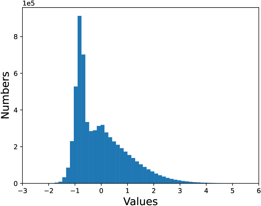
(a) Art painting

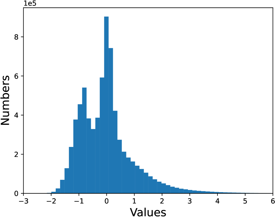
(b) Cartoon

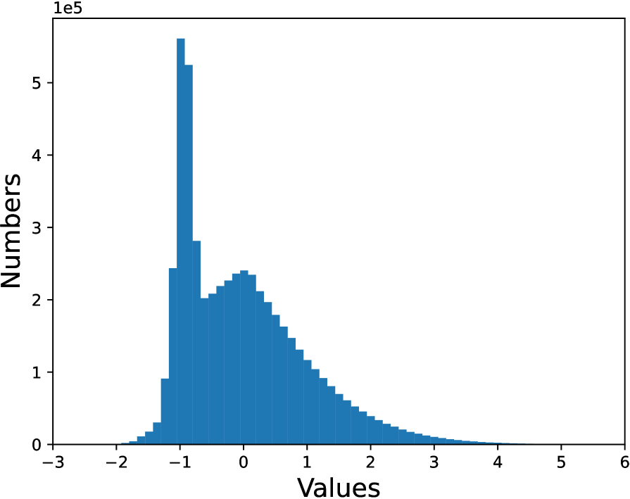
(c) Photo

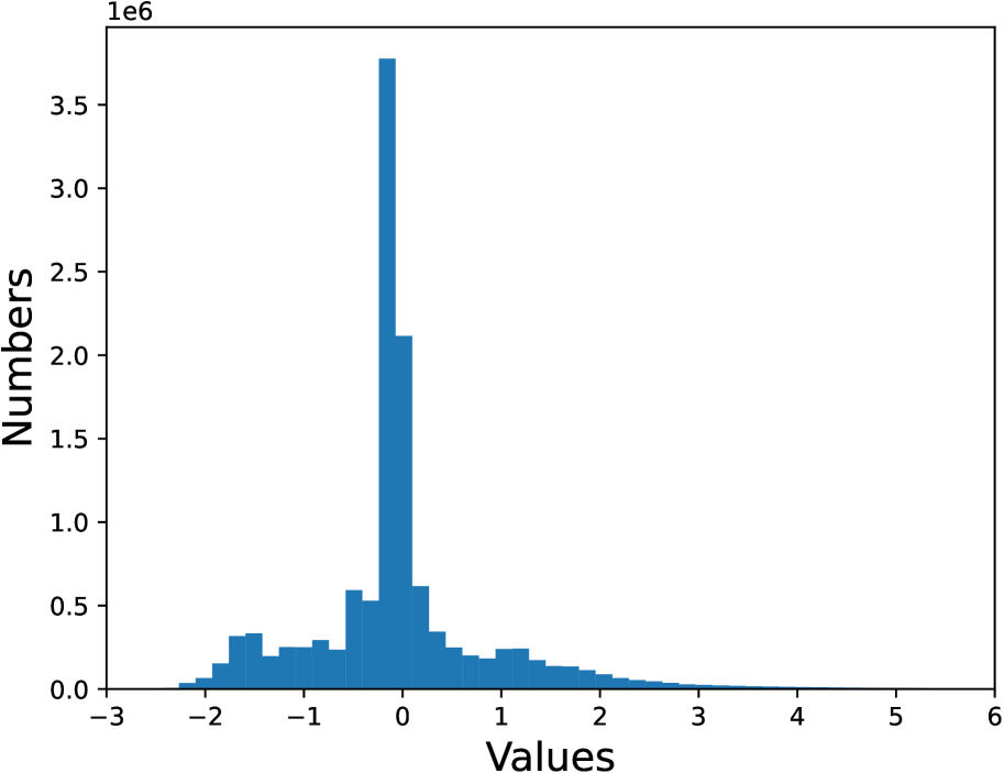
(d) Sketch

Figure 1: Histograms of feature values in a randomly selected channel, where features are computed from the first residual block of a ResNet-18 [20] trained on the dataset of four domains [28]. We first normalize the mean and standard deviation of each channel to be $0$ and $1$, respectively, and then collect feature values among all test samples in each domain for visualization. One can clearly see that the feature distributions of real-world data are usually too complicated to be modeled by Gaussian.

Intuitively, EFDM can be done by matching the high-order statistics of features. Actually, high-order central moments have been explicitly introduced in [25, 63] to match distributions more precisely. However, considering high-order statistics in this way would introduce intensive computational overhead. Furthermore, the EFDM could only be theoretically achieved by matching central moments of infinite order [63], which is prohibitive in practice. Motivated by the Glivenko–Cantelli theorem [54], which states that the empirical Cumulative Distribution Function (eCDF) asymptotically converges to the Cumulative Distribution Function when the number of samples approaches infinity, Risser et al. [46] introduce the classical Histogram Matching (HM) [58, 16] method as an auxiliary measurement to minimize the feature distribution divergence. Unfortunately, HM can only approximately match eCDFs when there are equivalent feature values in inputs, since HM merges equivalent values as a single point and applies a point-wise transformation. (A toy example is illustrated in Fig. 2). This commonly happens for digital images with discrete integer values (e.g., 8-bits digital images). For features generated by deep models, equivalent feature values are also ineluctable due to their dependency on discrete image pixels and the use of activation functions, e.g., ReLU [42] and ReLU6 [26] (please refer to Fig. 3 for more details). All these facts impede the effectiveness of EFDM via HM.

To solve the above mentioned problem, we, for the first time to our best knowledge, propose to perform EFDM by exactly matching the eCDFs of image features, resulting in exactly matched feature distributions (when the number of samples approaches infinity) and consequently exactly matched mean, standard deviation, and high-order statistics (see the toy example in Fig. 2). The exact matching of eCDFs can be implemented by applying the Exact Histogram Matching (EHM) algorithm [18, 7] in the feature space. Specifically, by distinguishing the equivalent feature values and applying an element-wise transformation, EHM conducts more fine-grained and more accurate matching of eCDFs than HM. In this paper, a fast EHM algorithm, named Sort-Matching [47], is adopted to perform EFDM in a plug-and-play manner with minimal cost.

With EFDM, we conduct cross-distribution feature matching in one shot (cf. Eq. 6) and propose a new style loss (cf. Eq. 9) to more accurately measure distribution divergence, producing more stable style-transfer images in AST. Following [72], we extend EFDM to generate feature augmentations with mixed styles, leading to the Exact Feature Distribution Mixing (EFDMix) (cf. Eq. 10), which can provide more diverse feature augmentations for DG applications. Our method achieves new state-of-the-arts on a variety of AST and DG tasks with high efficiency.

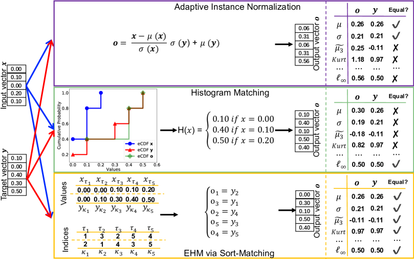
Figure 2: A comparison between AdaIN, HM and EHM via Sort-Matching using a toy example, where value precision is rounded to the level of 0.01. AdaIN only matches the mean and standard deviation between output vector ${\bm{o}}$ and target vector ${\bm{y}}$. Although the eCDF of ${\bm{o}}$ is approximated to that of ${\bm{y}}$ by HM, they are not exactly matched, leading to the mismatched distributions and, consequently, the mismatched statistics. The EHM via Sort-Matching exactly matches the eCDFs of ${\bm{o}}$ and ${\bm{y}}$, resulting in exactly matched distributions and, consequently, exactly matched statistics. Notations of $\mu,\sigma,\widetilde{\mu_{3}}$, $Kurt$ and $\ell_{\infty}$ indicate the mean, standard deviation, third standardized moment-skewness [60, 24], fourth standardized moment-kurtosis [59, 24], and infinite norm, respectively.

2 Related Work

Arbitrary style transfer (AST) has been investigated in two conceptual directions: iterative optimization-based methods and feed-forward methods. The former [12, 46, 25] optimize image pixels in an iterative manner, whereas the latter [21, 33, 37, 41, 32] generate style-transferred output in one shot. Our method belongs to the latter one, which is generally faster and suitable for real-time applications. In both directions, transferring styles can be interpreted as a problem of feature distribution matching by assuming the image styles can be represented by feature distributions. Specifically, the seminal work in [12] adopts the second-order moments captured by the Gram matrix as the style representation. The loss introduced in [12] is rewritten as a Maximum Mean Discrepancy between image features in [34], bridging style transfer and feature distribution matching. Actually, many AST methods can be interpreted from the perspective of feature distribution matching. Based on the Gaussian prior assumption, feature distribution matching is conducted by matching mean and standard deviation in AdaIN [21]. Compared to AdaIN, WCT [33] additionally considers the covariance of feature channels via a pair of feature transforms, whitening and coloring. By additionally taking the content loss in [12] into the framework of WCT, a closed-form solution is presented in [37, 41, 32]. Besides the widely used first and second order feature statistics, high-order central moments and HM are introduced in [25] and [46] respectively for more exact distribution matching by relaxing the assumption of Gaussian feature distributions. However, computing high-order statistics explicitly introduces intensive computational overhead and the EFDM via HM is impeded by equivalent feature values. To this end, we, for the first time to our best knowledge, propose an accurate and efficient way for EFDM by exactly matching the eCDFs of image features, leading to more faithful AST results (please refer to Fig. 5 for visual examples).

Domain generalization (DG) aims to develop models that can generalize to unseen distributions. Typical DG methods include learning domain-invariant feature representations [40, 31, 15, 66, 5, 65, 67], meta-learning-based learning strategies [29, 9, 4], data augmentation [56, 61, 71, 13, 43, 72] and so on [57, 69]. Among all above methods, the recent state-of-the-art [72] augments cross-distribution features based on the feature distribution matching technique [21], which is introduced in the above AST part. By utilizing high-order statistics implicitly via the proposed EFDM method, more diverse feature augmentations can be achieved and significant performance improvements have been observed (please refer to Tabs. 1 and 2 for details).

Exact histogram matching (EHM) was proposed to match histograms of image pixels exactly. Compared to classical HM, EHM algorithms distinguish equivalent pixel values either randomly [48, 47] or according to their local mean [18, 7], leading to more accurate matching of histograms. The difference between outputs of EHM and HM in image pixel space is typically small, which is hardly perceptible to human eyes. However, this small difference can be amplified in the feature space of deep models, leading to clear divergence in feature distribution matching. We hence propose to perform EFDM by exactly matching the eCDFs of image features via EHM. While EHM can be conducted with different strategies, we empirically find that they yield similar results in our applications, and thus we promote the fast Sort-Matching [47] algorithm for EHM.

3 Methodology

3.1 AdaIN, HM and EHM

Adaptive instance normalization (AdaIN) [21] transforms an input vector ${\bm{x}}\in\mathbb{R}^{n}$, which is sampled from a random variable $X$, into an output vector ${\bm{o}}\in\mathbb{R}^{n}$, whose mean and standard deviation match those of a target vector ${\bm{y}}\in\mathbb{R}^{m}$ sampled from a random variable $Y$:

$${\bm{o}}=\frac{{\bm{x}}-\mu({\bm{x}})}{\sigma({\bm{x}})}\sigma({\bm{y}})+\mu({\bm{y}}),$$ (1)

where $\mu(\cdot)$ and $\sigma(\cdot)$ indicate the mean and standard deviation of referred data, respectively. By assuming that $X$ and $Y$ follow Gaussian distributions and $n$ and $m$ approach infinity, AdaIN can achieve EFDM by matching feature mean and standard deviation [37, 41, 32]. However, feature distributions of real-world data usually deviate much from Gaussian, as can be seen from Fig. 1. Therefore, matching feature distributions by AdaIN is less accurate.

Histogram matching (HM) [58, 16] aims to transform an input vector ${\bm{x}}$ into an output vector ${\bm{o}}$, whose eCDF matches the target eCDF of a target vector ${\bm{y}}$. The eCDFs of ${\bm{x}}$ and ${\bm{y}}$ are defined as:

$$\widehat{F}_{X}(x)=\frac{1}{n}\sum\nolimits_{i=1}^{n}\mathbf{1}_{x_{i}\leq x},\quad\widehat{F}_{Y}(y)=\frac{1}{m}\sum\nolimits_{i=1}^{m}\mathbf{1}_{y_{i}\leq y},$$ (2)

where $\mathbf{1}_{A}$ is the indicator of event $A$ and $x_{i}$ (or $y_{i}$) is the $i$-th element of ${\bm{x}}$ (or ${\bm{y}}$). For each element $x_{i}$ of the input vector ${\bm{x}}$, we find the $y_{j}$ that satisfies $\widehat{F}_{X}(x_{i})=\widehat{F}_{Y}(y_{j})$, resulting in the transformation function: $H(x_{i})=y_{j}$. One may opt to match the explicit histograms as in discrete image space [16]. It is worth mentioning that matching eCDFs is equivalent to matching histograms with bins of infinitesimal width, which is however hard to achieve due to the finite number of bits to represent features.

Ideally, HM could exactly match eCDFs of image features in the continuous case. Unfortunately, HM can only approximately match eCDFs when there exist equivalent feature values in inputs, since HM merges equivalent values as a single point and applies a point-wise transformation (please refer to the toy example in Fig. 2). For features generated by deep models, equivalent feature values are common due to their dependency on discrete image pixels and the use of activation functions, e.g., ReLU [42] and ReLU6 [26] (please refer to Fig. 3 for more details). All these facts impede the effectiveness of EFDM via HM.

Exact Histogram Matching (EHM) [18, 7] was proposed to match histograms of image pixels exactly. Different from HM, EHM algorithms distinguish equivalent pixel values and apply an element-wise transformation so that a more accurate histogram matching can be achieved. While EHM can be conducted with different strategies, we adopt the Sort-Matching algorithm [47] for its fast speed. Sort-Matching is based on the quicksort strategy [49], which is generally accepted as the fastest sort algorithm with complexity of $O(n\log n)$. As stated by its name, Sort-Matching is implemented by matching two sorted vectors, whose indexes are illustrated in a one-line notation [2] as:

$$\begin{split}&{\bm{x}}:\tau=\left(\begin{array}[]{ccccc}\tau_{1}&\tau_{2}&\tau_{3}&\cdots&\tau_{n}\end{array}\right),\\ &{\bm{y}}:\kappa=\left(\begin{array}[]{ccccc}\kappa_{1}&\kappa_{2}&\kappa_{3}&\cdots&\kappa_{n}\end{array}\right),\end{split}$$ (3)

where $\{x_{\tau_{i}}\}_{i=1}^{n}$ and $\{y_{\kappa_{i}}\}_{i=1}^{n}$ are sorted values of ${\bm{x}}$ and ${\bm{y}}$ in ascending order. In other words, ${x}_{\tau_{1}}=\min({\bm{x}})$, ${x}_{\tau_{n}}=\max({\bm{x}})$, and ${x}_{\tau_{i}}\leq{x}_{\tau_{j}}$ if $i<j$. ${y}_{\kappa_{i}}$ is similarly defined. Based on the definition in Eq. 3, Sort-Matching outputs ${\bm{o}}$ with its $\tau_{i}$-th element ${o}_{\tau_{i}}$ as:

$${o}_{\tau_{i}}={y}_{\kappa_{i}}.$$ (4)

Compared to AdaIN, HM and other EHM algorithms [18, 7], Sort-Matching additionally assumes that the two vectors to be matched are of the same size, i.e. $m=n$, which is satisfied in our focused applications of AST and DG. In other applications where the two vectors are of different sizes, interpolation or dropping elements can be conducted to make ${\bm{y}}$ and ${\bm{x}}$ the same size.

3.2 EFDM for AST and DG

In this section, we apply EFDM to tasks of AST and DG. We conduct the exact eCDFs matching by applying the EHM algorithm via Sort-Matching in the image feature space. To enable the gradient back-propagation in deep models, we practically perform EFDM by modifying Eq. 4 as:

$$\textrm{EFDM}({\bm{x}},{\bm{y}}):{o}_{\tau_{i}}={x}_{\tau_{i}}+{y}_{\kappa_{i}}-\langle{x}_{\tau_{i}}\rangle,$$ (5)

where $\langle\cdot\rangle$ represents the stop-gradient operation [6]. We stop the gradients to the style feature ${y}_{\kappa_{i}}$ following [21, 72]. Given the input data ${\bm{X}}\in\mathbb{R}^{B\times C\times HW}$ and the style data ${\bm{Y}}\in\mathbb{R}^{B\times C\times HW}$, we apply EFDM in a channel-wise manner following [21, 72], where $B,C,H,W$ indicate batch size, channel dimension, height, and width, respectively. The proposed EFDM does not introduce any parameters and can be used in a plug-and-play manner with few lines of codes and minimal cost, as summarized in Algorithm 1.

Algorithm 1 PyTroch-like pseudo-code for EFDM.

# ${\bm{x}}$, ${\bm{y}}$: input and target vectors of the same shape (n)
_, IndexX = torch.sort(${\bm{x}}$)      # Sort ${\bm{x}}$ values
SortedY, _ = torch.sort(${\bm{y}}$)     # Sort ${\bm{y}}$ values
InverseIndex = IndexX.argsort(-1)
return ${\bm{x}}$ + SortedY.gather(-1, InverseIndex) - ${\bm{x}}$.detach()

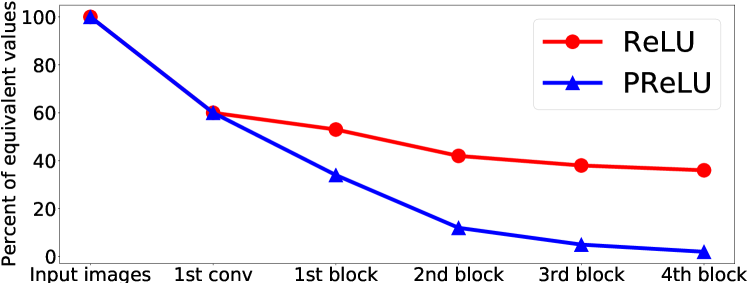
Figure 3: An illustration of the percent of equivalent feature values (i.e., $\frac{\textrm{number of equivalent values}}{\textrm{number of all values}}*100$) in ResNet18 feature maps with an input image of resolution $224\times 224$ . ‘1st conv’ represents the output of the first convolution layer. ‘1st block’, ‘2nd block’, ‘3rd block’, and ‘4th block’ indicate the outputs of the 1st, 2nd, 3rd, and 4th residual blocks, respectively. ‘ReLU’ and ‘PReLU’ indicate the vanilla ResNet18 with ReLU [42] and PReLU [19] activation functions, respectively. The percentage depends on the number of bits to represent the feature values and the size of feature maps. In the original image pixel space, the percentage is close to 100 percent since the pixels are quantized into 8-bits. The percentage decreases in the floating number (32-bits) feature space, as well as the depth of blocks since deeper blocks have smaller feature maps. In addition, compared to PReLU, there are generally more equivalent feature values for models with ReLU, since the ReLU function sets all negative values to zero.

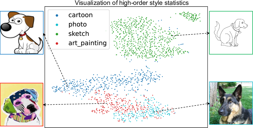
Figure 4: t-SNE [53] visualization of the third standardized moment-skewness [60, 24], which clearly shows that the style information can be represented by high-order statistics beyond mean and standard deviation. Besides skewness, style information can also be observed in the fourth standardized moment-kurtosis [59, 24] and infinite norm (please refer to the supplementary file for details). The visualized features are extracted from the 1st residual block of ResNet-18 [20] trained on the dataset of four domains [28].

EFDM for AST. A simple encoder-decoder architecture is adopted, where we fix the encoder $f$ as the first few layers (up to $relu4\_1$) of a pre-trained VGG-19 [51]. Given the content images ${\bm{X}}$ and style images ${\bm{Y}}$, we first encode them to the feature space and apply EFDM to get the style-transferred features as:

$${\bm{S}}=\textrm{EFDM}(f({\bm{X}}),f({\bm{Y}})).$$ (6)

Then, we train a randomly initialized decoder $g$ to map ${\bm{S}}$ to the image space, resulting in the stylized images $g({\bm{S}})$. Following [21, 10], we train the decoder with the weighted combination of a content loss $\mathcal{L}_{c}$ and a style loss $\mathcal{L}_{s}$, leading to the following objective:

$$\mathcal{L}=\mathcal{L}_{c}+\omega\mathcal{L}_{s},$$ (7)

where $\omega$ is a hyper-parameter balancing the two loss terms. Specifically, the content loss $\mathcal{L}_{c}$ is the Euclidean distance between features of stylized images $f(g({\bm{S}}))$ and the style-transferred features ${\bm{S}}$:

$$\mathcal{L}_{c}=\|f(g({\bm{S}}))-{\bm{S}}\|_{2}.$$ (8)

The style loss measures the distribution divergence between features of the stylized images $g({\bm{S}})$ and style images ${\bm{Y}}$, which is instantiated as their divergence on mean and standard deviation in [21] based on the Gaussian prior. To measure the distribution divergence more exactly, we introduce the style loss as the sum of Euclidean distance between features of the stylized images $\phi_{i}(g({\bm{S}}))$ and its style-transferred target $\textrm{EFDM}(\phi_{i}(g({\bm{S}})),\phi_{i}({\bm{Y}}))$:

$$\mathcal{L}_{s}=\sum\nolimits_{i=1}^{L}\|\phi_{i}(g({\bm{S}}))-\textrm{EFDM}(\phi_{i}(g({\bm{S}})),\phi_{i}({\bm{Y}}))\|_{2}.$$ (9)

Following [21], we instantiate $\{\phi_{i}\}_{i=1}^{L}$ as $relu1\_1$, $relu2\_1$, $relu3\_1$, and $relu4\_1$ layers in VGG-19.

EFDM for DG. Inspired by the studies that style information can be represented by the mean and standard deviation of image features [21, 33, 37], Zhou et al. [72] proposed to generate style-transferred and content-preserved feature augmentations for DG problems. As we discussed before, distributions beyond Gaussian have high-order statistics other than mean and standard deviation, and hence the style information can be more accurately represented by using high-order feature statistics. The visualization in Fig. 4 demonstrates that the third standardized moment-skewness [60, 24] can well represent the four different domains of the same object. This motivates us to utilize high-order statistics for feature augmentations in DG.

Since high-order feature statistics can be efficiently and implicitly matched via our proposed EFDM method, it is a natural idea to replace AdaIN with EFDM for cross-distribution feature augmentation in DG. To generate more diverse feature augmentations with mixed styles, following [72] we extend the EFDM in Eq. 5 by interpolating sorted vectors, resulting in the Exact Feature Distribution Mixing (EFDMix) as:

$$\textrm{EFDMix}({\bm{x}},{\bm{y}}):{o}_{\tau_{i}}={x}_{\tau_{i}}+(1-\lambda){y}_{\kappa_{i}}-(1-\lambda)\langle{x}_{\tau_{i}}\rangle.$$ (10)

The instance-wise mixing weight $\lambda$ is adopted and we sample $\lambda$ from the Beta-distribution: $\lambda\sim Beta(\alpha,\alpha)$, where $\alpha\in(0,\infty)$ is a hyper-parameter. We set $\alpha=0.1$ unless otherwise specified. Obviously, EFDMix degenerates to EFDM when $\lambda=0$.

Given the input feature ${\bm{X}}$, following [72] we adopt two strategies to mix with the style feature ${\bm{Y}}$. When domain labels are given, we sample ${\bm{Y}}$ from a domain different from that of ${\bm{X}}$, leading to EFDMix w/ domain label. Otherwise, ${\bm{Y}}$ is obtained by shuffling ${\bm{X}}$ along the batch dimension, resulting in EFDMix w/ random shuffle. We train the model solely with the cross-entropy loss. Following [72], we insert the EFDMix module to multiple lower-level layers, adopt a probability of $0.5$ to decide whether the EFDMix is activated in the forward pass of training stage, and deactivate it in the testing stage.

The advantage of utilizing high-order feature statistics could be intuitively clarified by the augmentation diversity. For example, given two different style features $\widehat{{\bm{y}}}$ and $\widetilde{{\bm{y}}}$ with the same mean and standard deviation and a specific mixing weight $\lambda$, the same augmented feature will be obtained by only utilizing the mean and standard deviation [72]. On the contrary, our EFDMix could generate two different augmentations by implicitly utilizing high-order statistics, resulting in more diverse feature augmentations.

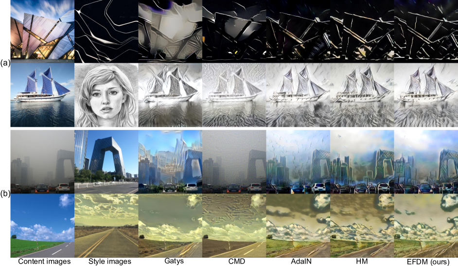
Figure 5: Illustration of results on (a) style transfer [21] (top two rows) and (b) the more challenging photo-realistic style transfer [38] (bottom two rows) tasks. Results of ‘Gatys’ [12] and ‘CMD’ [25] are obtained with official codes. For HM, we use HM, instead of EHM, to approximately match eCDFs. More visualizations are provided in the supplementary file.

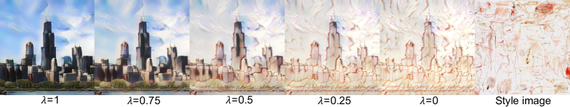
Figure 6: Visualization of content-style trade-off with various $\lambda$ in Eq. 10.

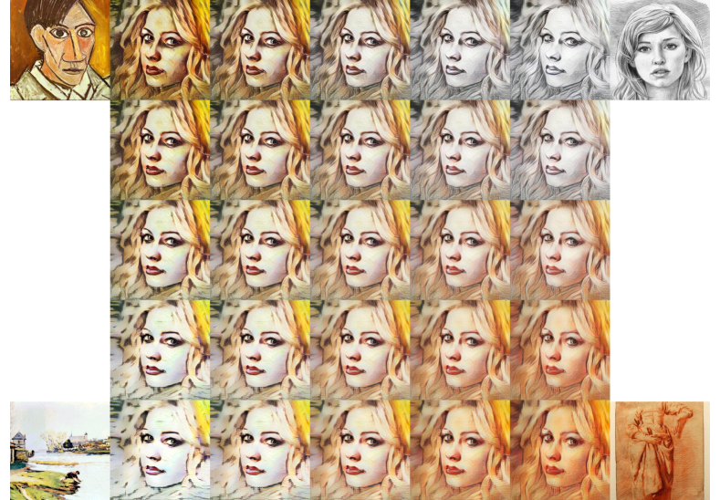
Figure 7: Visualization of style interpolation.

4 Experiments

We perform experiments on AST and DG tasks to validate the effectiveness of EFDM.

4.1 Experiments on AST

We closely follow [21] to conduct the experiments on AST. Specifically, we adopt the adam optimizer, set the batch size as $8$ content-style image pairs, and set the hyper-parameter $\omega=10$. In training, the MS-COCO [35] and WikiArt [44] are adopted as the content and style images, respectively. We compare EFDM with state-of-the-arts in Fig. 5. One can see that our EFDM works stably across the style transfer (top two rows) and the more challenging photo-realistic style transfer (bottom two rows) tasks. By conducting feature distribution matching more exactly, it preserves more faithfully the image structures and details while transferring the style, and produces more photo-realistic results. In contrary, the competing methods may introduce many visual artifacts and image distortions. More visual results can be found in the supplementary file.

Content-style trade-off in the test stage. The trade-off between content and style could be achieved by adjusting the hyper-parameter $\omega$ in Eq. 7. Additionally, we could manipulate the content-style trade-off by interpolating between the content feature and style feature, which can be achieved with the EFDMix in Eq. 10. The vanilla content image is expected when $\lambda=1$ and the model would output the most stylized image when $\lambda=0$. We illustrate an example in Fig. 6. We see that the images transition smoothly from the content style to target style by varying $\lambda$ from 1 to 0.

Style interpolation. Following [21], we interpolate feature maps to interpolate the $K$ style images ${\bm{Y}}_{1}$, ${\bm{Y}}_{2}$, $\cdots$, ${\bm{Y}}_{K}$ with corresponding weights $w_{1},w_{2},\cdots,w_{K}$ as follows:

$$g\left(\sum\nolimits_{k=1}^{K}w_{k}\textrm{EFDM}({\bm{X}},{\bm{Y}}_{k})\right),$$ (11)

where $\sum_{k=1}^{K}w_{k}=1$. As illustrated in Fig. 7, new styles can be obtained by such style interpolation.

Method	Art	Cartoon	Photo	Sketch	Avg
Leave-one-domain-out generalization results
JiGen [3]	79.4	75.3	96.0	71.6	80.5
L2A-OT [71]	83.3	78.2	96.2	73.6	82.8
ResNet-18 [20]	77.0$\pm$0.6	75.9$\pm$0.6	96.0$\pm$0.1	69.2$\pm$0.6	79.5
+ Mixup [64]	76.8$\pm$0.7	74.9$\pm$0.7	95.8$\pm$0.3	66.6$\pm$0.7	78.5
+ MixStyle w/ domain label [72]	83.1$\pm$0.8	78.6$\pm$0.9	95.9$\pm$0.4	74.2$\pm$2.7	82.9
+ EFDMix w/ domain label (ours)	83.9$\pm$0.4	79.4$\pm$0.7	96.8$\pm$0.4	75.0$\pm$0.7	83.9
ResNet-50 [20]	84.4$\pm$0.9	77.1$\pm$1.4	97.6$\pm$0.2	70.8$\pm$0.7	82.5
+ MixStyle w/ domain label [72]	90.3$\pm$0.3	82.3$\pm$0.7	97.7$\pm$0.4	74.7$\pm$0.7	86.2
+ EFDMix w/ domain label (ours)	90.6$\pm$0.3	82.5$\pm$0.7	98.1$\pm$0.2	76.4$\pm$1.2	86.9
Single source generalization results
ResNet-18 [20]	58.6$\pm$2.4	66.4$\pm$0.7	34.0$\pm$1.8	27.5$\pm$4.3	46.6
+ MixStyle w/ random shuffle [72]	61.9$\pm$2.2	71.5$\pm$0.8	41.2$\pm$1.8	32.2$\pm$4.1	51.7
+ EFDMix w/ random shuffle (ours)	63.2$\pm$2.3	73.9$\pm$0.7	42.5$\pm$1.8	38.1$\pm$3.7	54.4
ResNet-50 [20]	63.5$\pm$1.3	69.2$\pm$1.6	38.0$\pm$0.9	31.4$\pm$1.5	50.5
+ MixStyle w/ random shuffle [72]	73.2$\pm$1.1	74.8$\pm$1.1	46.0$\pm$2.0	40.6$\pm$2.0	58.6
+ EFDMix w/ random shuffle (ours)	75.3$\pm$0.9	77.4$\pm$0.8	48.0$\pm$0.9	44.2$\pm$2.4	61.2

Table 1: Domain generalization results of category classification on PACS. Results of MixStyle are obtained with official codes. The listed domain is the test domain in the leave-one-domain-out setting, while it is the training one in the single source generalization setting.

Methods	MarKet1501$\to$GRID				GRID$\to$MarKet1501
	mAP	R1	R5	R10	mAP	R1	R5	R10
OSNet [70]	33.3$\pm$0.4	24.5$\pm$0.4	42.1$\pm$1.0	48.8$\pm$0.7	3.9$\pm$0.4	13.1$\pm$1.0	25.3$\pm$2.2	31.7$\pm$2.0
+ MixStyle w/ random shuffle [72]	33.8$\pm$0.9	24.8$\pm$1.6	43.7$\pm$2.0	53.1$\pm$1.6	4.9$\pm$0.2	15.4$\pm$1.2	28.4$\pm$1.3	35.7$\pm$0.9
+ EFDMix w/ random shuffle (ours)	35.5$\pm$1.8	26.7$\pm$3.3	44.4$\pm$0.8	53.6$\pm$2.0	6.4$\pm$0.2	19.9$\pm$0.6	34.4$\pm$1.0	42.2$\pm$0.8

Table 2: Domain generalization results on the cross-domain person re-ID task. Results of MixStyle are obtained with official codes.

4.2 Experiments on DG

We closely follow MixStyle [72] to conduct experiments on DG, including data preparing, model training and selection. In other words, we only replace the MixStyle module with EFDMix, which is detailed as follows.

Generalization on category classification. We adopt the popular DG benchmark dataset of PACS [28], which includes $9,991$ images shared by $7$ classes and $4$ domains, i.e., Art, Cartoon, Photo, and Sketch. Two task settings are adopted. In the leave-one-domain-out setting [28], we train the model on three domains and test on the remaining one. In the single source DG [56, 45], models are trained on one domain and tested on the remaining three. We adopt ResNet-18 and ResNet-50, which are pre-trained on the ImageNet dataset, as the backbones.

We compare our method with the latest state-of-the-art MixStyle [72], the regularization based methods [64, 55, 14, 62, 8] and the representative DG methods [40, 31, 3, 50, 1, 30, 71]. Due to the limit of space, only partial results are reported in Tab. 1 and more comprehensive results are given in the supplementary file. One can see that our EFDMix consistently outperforms MixStyle, as well as other competing methods, on both settings. More advantages over the competing methods can be observed on the single source generalization setting, where the training data have less diversity. This can be explained by the more diverse feature augmentations via EFDMix, as clarified in Sec. 3.2.

We note there are different experimental strategies in the DG community. Following the recent DomainBed [17], our EFDMix achieves 87.9% accuracy on the PACS dataset, outperforming the strong ERM benchmark [17] by 1.2%. Please refer to the supplementary file for details.

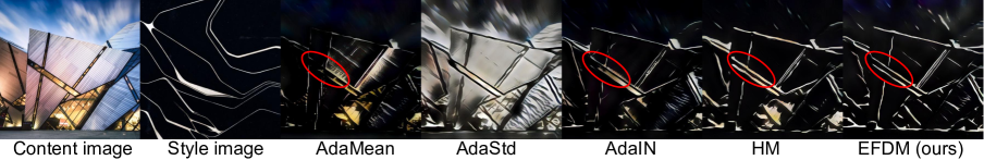
Figure 8: Qualitative analyses on the role of different orders of feature statistics on AST.

Generalization on instance retrieval. We adopt the person re-identification (re-ID) datasets of Markert1501 [68] and GRID [36] to conduct cross-domain instance retrieval. We follow [72] to conduct experiments with the OSNet [70]. Similar to the findings in classification, EFDMix outperforms MixStyle and other competitors, as shown in Tab. 2. This once again validates the effectiveness of utilizing high-order statistics for feature augmentations in DG.

4.3 Discussions

The role of different orders of feature statistics. To make further investigation on the role of different orders of feature statistics, we implement AdaIN by matching only feature mean and standard deviation, resulting in the AdaMean and AdaStd variants of it. (Please refer to the supplementary file for details.) The qualitative results on AST and the quantitative results on DG are illustrated in Fig. 8 and Fig. 9, respectively. From Fig. 8, we can see that AdaMean roughly matches the basic color tone. AdaStd preserves the structure of the content image but with wrong color tone. By matching both mean and standard deviation, AdaIN preserves more details and correct tone. With the implicitly matched high-order feature statistics, EFDM preserves the most content details. From Fig. 9, we see that performing feature augmentation with either AdaMean or AdaStd could improve over the ResNet-50 baseline, while AdaMean performs slightly better. AdaIN outperforms AdaMean and AdaStd by more than $1\%$, justifying the effectiveness of utilizing more feature statistics. By matching high-order feature statistics implicitly, EFDM achieves the best result. Though HM approximately matches eCDFs, it cannot even ensure the exact matching of mean and standard deviation, leading to degenerated performance.

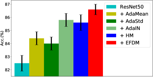
Figure 9: Quantitative analyses on the role of different orders of feature statistics on PACS dataset.

User study on style transfer. As shown in Tab. 3, our method receives the most votes for its better stylized performance across competing AST methods. Please refer to the supplementary file for more details.

EFDM with different EHM algorithms. Different EHM algorithms are distinguished by their sort strategies of equivalent values. In Fig. 10, we implement EFDM with different EHM algorithms on the task of DG. One can see that they yield similar accuracies on the PACS dataset. Considering that the quicksort-empowered Sort-Matching has the fastest speed, we adopt it for EFDM in our work.

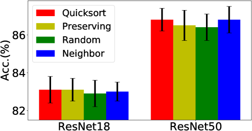
Figure 10: Results on PACS dataset with different implementations of EFDM. Besides Sort-Matching with Quicksort [49], we preserve the order of equivalent values in ${\bm{x}}$ (Preserving), randomly sort equivalent values [48] (Random), and sort equivalent values according to their local mean [18] (Neighbor) to implement EFDM, respectively. We see that the different implementations lead to similar results.

Methods	Gatys [12]	CMD [25]	HM	EFDM	AdaIN
Time (s)	25.61	19.84	0.33	0.0039	0.0038
Percent (%)	19.9	12.2	17.1	29.8	21.0

Table 3: Average running time and user preference across competing AST methods. The running time is averaged on 512$\times$512 images with a Tesla V100 GPU.

Running time. We evaluate the speed of our EFDM method on the AST task. The average running time of different algorithms to process a 512$\times$512 image is listed in Tab. 3. EFDM is significantly faster than methods in [12, 25] and the HM based algorithm, which is implemented with the skimage library. It has nearly the same speed as the seminal AdaIN [21] and runs at 256 FPS for images of size 512 $\times$ 512, making it applicable for real-time applications.

Limitations. Compared to AdaIN [21] with linear complexity, EFDM has a higher complexity of $n\log(n)$. Fortunately, due to the finite feature size, its running time is comparable to AdaIN on the AST and DG tasks. In addition, following [21, 25, 72], we assume that different feature channels are independent, which is not exactly true and is challenged by [33, 37].

More discussions on EFDMix, EFDM vs. EFDMix, the selection of $\alpha$ in Eq. 10, loss curves, the influence of ReLU functions, the comparison to related methods on DG [72, 52, 23, 11], and the detailed analysis on computation time can be found in the supplementary file.

5 Conclusion

We made the first attempt, to our best knowledge, to perform exact matching of feature distributions, and applied the so-called exact feature distribution matching (EFDM) method to applications of AST and DG. We employed a fast EHM algorithm, i.e., Sort-Matching, to implement EFDM in the deep feature space. The proposed EFDM method demonstrated superior performance to existing state-of-the-arts of AST and DG in terms of visual quality and quantitative measures. Our work opened a door to perform EFDM for visual learning tasks efficiently. Extensive investigations could be followed up, e.g., empowering classical normalization [22] beyond statistics of mean and standard deviation.

References

- [1] Yogesh Balaji, Swami Sankaranarayanan, and Rama Chellappa. Metareg: Towards domain generalization using meta-regularization. Advances in Neural Information Processing Systems, 31:998–1008, 2018.
- [2] Kenneth P Bogart. Introductory combinatorics. Saunders College Publishing, 1989.
- [3] Fabio M Carlucci, Antonio D’Innocente, Silvia Bucci, Barbara Caputo, and Tatiana Tommasi. Domain generalization by solving jigsaw puzzles. In Proceedings of the IEEE/CVF Conference on Computer Vision and Pattern Recognition, pages 2229–2238, 2019.
- [4] Chaoqi Chen, Jiongcheng Li, Xiaoguang Han, Xiaoqing Liu, and Yizhou Yu. Compound domain generalization via meta-knowledge encoding. In Proceedings of the IEEE/CVF Conference on Computer Vision and Pattern Recognition, 2022.
- [5] Chaoqi Chen, Weiping Xie, Wenbing Huang, Yu Rong, Xinghao Ding, Yue Huang, Tingyang Xu, and Junzhou Huang. Progressive feature alignment for unsupervised domain adaptation. In Proceedings of the IEEE/CVF Conference on Computer Vision and Pattern Recognition, pages 627–636, 2019.
- [6] Xinlei Chen and Kaiming He. Exploring simple siamese representation learning. In Proceedings of the IEEE/CVF Conference on Computer Vision and Pattern Recognition, pages 15750–15758, 2021.
- [7] Dinu Coltuc, Philippe Bolon, and J-M Chassery. Exact histogram specification. IEEE Transactions on Image Processing, 15(5):1143–1152, 2006.
- [8] Terrance DeVries and Graham W Taylor. Improved regularization of convolutional neural networks with cutout. arXiv preprint arXiv:1708.04552, 2017.
- [9] Yingjun Du, Jun Xu, Huan Xiong, Qiang Qiu, Xiantong Zhen, Cees GM Snoek, and Ling Shao. Learning to learn with variational information bottleneck for domain generalization. In European Conference on Computer Vision, pages 200–216. Springer, 2020.
- [10] Vincent Dumoulin, Jonathon Shlens, and Manjunath Kudlur. A learned representation for artistic style. ICLR, 2017.
- [11] Xinjie Fan, Qifei Wang, Junjie Ke, Feng Yang, Boqing Gong, and Mingyuan Zhou. Adversarially adaptive normalization for single domain generalization. In Proceedings of the IEEE/CVF Conference on Computer Vision and Pattern Recognition, pages 8208–8217, 2021.
- [12] Leon A Gatys, Alexander S Ecker, and Matthias Bethge. Image style transfer using convolutional neural networks. In Proceedings of the IEEE conference on computer vision and pattern recognition, pages 2414–2423, 2016.
- [13] Robert Geirhos, Patricia Rubisch, Claudio Michaelis, Matthias Bethge, Felix A Wichmann, and Wieland Brendel. Imagenet-trained cnns are biased towards texture; increasing shape bias improves accuracy and robustness. ICLR, 2019.
- [14] Golnaz Ghiasi, Tsung-Yi Lin, and Quoc V Le. Dropblock: A regularization method for convolutional networks. arXiv preprint arXiv:1810.12890, 2018.
- [15] Rui Gong, Wen Li, Yuhua Chen, and Luc Van Gool. Dlow: Domain flow for adaptation and generalization. In Proceedings of the IEEE/CVF Conference on Computer Vision and Pattern Recognition, pages 2477–2486, 2019.
- [16] Rafael C Gonzalez, Richard E Woods, et al. Digital image processing, 2002.
- [17] Ishaan Gulrajani and David Lopez-Paz. In search of lost domain generalization. ICLR, 2021.
- [18] Ernest L Hall. Almost uniform distributions for computer image enhancement. IEEE Transactions on Computers, 100(2):207–208, 1974.
- [19] Kaiming He, Xiangyu Zhang, Shaoqing Ren, and Jian Sun. Delving deep into rectifiers: Surpassing human-level performance on imagenet classification. In Proceedings of the IEEE international conference on computer vision, pages 1026–1034, 2015.
- [20] Kaiming He, Xiangyu Zhang, Shaoqing Ren, and Jian Sun. Deep residual learning for image recognition. In Proceedings of the IEEE conference on computer vision and pattern recognition, pages 770–778, 2016.
- [21] Xun Huang and Serge Belongie. Arbitrary style transfer in real-time with adaptive instance normalization. In Proceedings of the IEEE International Conference on Computer Vision, pages 1501–1510, 2017.
- [22] Sergey Ioffe and Christian Szegedy. Batch normalization: Accelerating deep network training by reducing internal covariate shift. In International conference on machine learning, pages 448–456. PMLR, 2015.
- [23] Xin Jin, Cuiling Lan, Wenjun Zeng, Zhibo Chen, and Li Zhang. Style normalization and restitution for generalizable person re-identification. In proceedings of the IEEE/CVF conference on computer vision and pattern recognition, pages 3143–3152, 2020.
- [24] Derrick N Joanes and Christine A Gill. Comparing measures of sample skewness and kurtosis. Journal of the Royal Statistical Society: Series D (The Statistician), 47(1):183–189, 1998.
- [25] Nikolai Kalischek, Jan D Wegner, and Konrad Schindler. In the light of feature distributions: moment matching for neural style transfer. In Proceedings of the IEEE/CVF Conference on Computer Vision and Pattern Recognition, pages 9382–9391, 2021.
- [26] Alex Krizhevsky and Geoff Hinton. Convolutional deep belief networks on cifar-10. Unpublished manuscript, 40(7):1–9, 2010.
- [27] Alex Krizhevsky, Ilya Sutskever, and Geoffrey E Hinton. Imagenet classification with deep convolutional neural networks. Advances in neural information processing systems, 25:1097–1105, 2012.
- [28] Da Li, Yongxin Yang, Yi-Zhe Song, and Timothy M Hospedales. Deeper, broader and artier domain generalization. In Proceedings of the IEEE international conference on computer vision, pages 5542–5550, 2017.
- [29] Da Li, Yongxin Yang, Yi-Zhe Song, and Timothy M Hospedales. Learning to generalize: Meta-learning for domain generalization. In Thirty-Second AAAI Conference on Artificial Intelligence, 2018.
- [30] Da Li, Jianshu Zhang, Yongxin Yang, Cong Liu, Yi-Zhe Song, and Timothy M Hospedales. Episodic training for domain generalization. In Proceedings of the IEEE/CVF International Conference on Computer Vision, pages 1446–1455, 2019.
- [31] Haoliang Li, Sinno Jialin Pan, Shiqi Wang, and Alex C Kot. Domain generalization with adversarial feature learning. In Proceedings of the IEEE Conference on Computer Vision and Pattern Recognition, pages 5400–5409, 2018.
- [32] Pan Li, Lei Zhao, Duanqing Xu, and Dongming Lu. Optimal transport of deep feature for image style transfer. In Proceedings of the 2019 4th International Conference on Multimedia Systems and Signal Processing, pages 167–171, 2019.
- [33] Yijun Li, Chen Fang, Jimei Yang, Zhaowen Wang, Xin Lu, and Ming-Hsuan Yang. Universal style transfer via feature transforms. arXiv preprint arXiv:1705.08086, 2017.
- [34] Yanghao Li, Naiyan Wang, Jiaying Liu, and Xiaodi Hou. Demystifying neural style transfer. IJCAI, 2017.
- [35] Tsung-Yi Lin, Michael Maire, Serge Belongie, James Hays, Pietro Perona, Deva Ramanan, Piotr Dollár, and C Lawrence Zitnick. Microsoft coco: Common objects in context. In European conference on computer vision, pages 740–755. Springer, 2014.
- [36] Chen Change Loy, Tao Xiang, and Shaogang Gong. Multi-camera activity correlation analysis. In 2009 IEEE Conference on Computer Vision and Pattern Recognition, pages 1988–1995. IEEE, 2009.
- [37] Ming Lu, Hao Zhao, Anbang Yao, Yurong Chen, Feng Xu, and Li Zhang. A closed-form solution to universal style transfer. In Proceedings of the IEEE/CVF International Conference on Computer Vision, pages 5952–5961, 2019.
- [38] Fujun Luan, Sylvain Paris, Eli Shechtman, and Kavita Bala. Deep photo style transfer. In Proceedings of the IEEE conference on computer vision and pattern recognition, pages 4990–4998, 2017.
- [39] Alexander McFarlane Mood. Introduction to the theory of statistics. 1950.
- [40] Saeid Motiian, Marco Piccirilli, Donald A Adjeroh, and Gianfranco Doretto. Unified deep supervised domain adaptation and generalization. In Proceedings of the IEEE international conference on computer vision, pages 5715–5725, 2017.
- [41] Youssef Mroueh. Wasserstein style transfer. arXiv preprint arXiv:1905.12828, 2019.
- [42] Vinod Nair and Geoffrey E Hinton. Rectified linear units improve restricted boltzmann machines. In Icml, 2010.
- [43] Hyeonseob Nam, HyunJae Lee, Jongchan Park, Wonjun Yoon, and Donggeun Yoo. Reducing domain gap by reducing style bias. In Proceedings of the IEEE/CVF Conference on Computer Vision and Pattern Recognition, pages 8690–8699, 2021.
- [44] K. Nichol. Painter by numbers, wikiart., 2016. https://www.kaggle.com/c/painter-by-numbers.
- [45] Fengchun Qiao, Long Zhao, and Xi Peng. Learning to learn single domain generalization. In Proceedings of the IEEE/CVF Conference on Computer Vision and Pattern Recognition, pages 12556–12565, 2020.
- [46] Eric Risser, Pierre Wilmot, and Connelly Barnes. Stable and controllable neural texture synthesis and style transfer using histogram losses. arXiv preprint arXiv:1701.08893, 2017.
- [47] Jannick P Rolland, V Vo, B Bloss, and Craig K Abbey. Fast algorithms for histogram matching: Application to texture synthesis. Journal of Electronic Imaging, 9(1):39–45, 2000.
- [48] Azriel Rosenfeld. Digital picture processing. Academic press, 1976.
- [49] Robert Sedgewick. Implementing quicksort programs. Communications of the ACM, 21(10):847–857, 1978.
- [50] Shiv Shankar, Vihari Piratla, Soumen Chakrabarti, Siddhartha Chaudhuri, Preethi Jyothi, and Sunita Sarawagi. Generalizing across domains via cross-gradient training. ICLR, 2018.
- [51] Karen Simonyan and Andrew Zisserman. Very deep convolutional networks for large-scale image recognition. arXiv preprint arXiv:1409.1556, 2014.
- [52] Zhiqiang Tang, Yunhe Gao, Yi Zhu, Zhi Zhang, Mu Li, and Dimitris N Metaxas. Crossnorm and selfnorm for generalization under distribution shifts. In Proceedings of the IEEE/CVF International Conference on Computer Vision, pages 52–61, 2021.
- [53] Laurens Van der Maaten and Geoffrey Hinton. Visualizing data using t-sne. Journal of machine learning research, 9(11), 2008.
- [54] Aad W Van der Vaart. Asymptotic statistics, volume 3. Cambridge university press, 2000.
- [55] Vikas Verma, Alex Lamb, Christopher Beckham, Amir Najafi, Ioannis Mitliagkas, David Lopez-Paz, and Yoshua Bengio. Manifold mixup: Better representations by interpolating hidden states. In International Conference on Machine Learning, pages 6438–6447. PMLR, 2019.
- [56] Riccardo Volpi, Hongseok Namkoong, Ozan Sener, John Duchi, Vittorio Murino, and Silvio Savarese. Generalizing to unseen domains via adversarial data augmentation. arXiv preprint arXiv:1805.12018, 2018.
- [57] Jindong Wang, Cuiling Lan, Chang Liu, Yidong Ouyang, Wenjun Zeng, and Tao Qin. Generalizing to unseen domains: A survey on domain generalization. IJCAI, 2021.
- [58] Wiki. Histogram matching. https://en.wikipedia.org/wiki/Histogram_matching.
- [59] Wiki. Kurtosis. https://en.wikipedia.org/wiki/Kurtosis.
- [60] Wiki. Skewness. https://en.wikipedia.org/wiki/Skewness.
- [61] Xiangyu Yue, Yang Zhang, Sicheng Zhao, Alberto Sangiovanni-Vincentelli, Kurt Keutzer, and Boqing Gong. Domain randomization and pyramid consistency: Simulation-to-real generalization without accessing target domain data. In Proceedings of the IEEE/CVF International Conference on Computer Vision, pages 2100–2110, 2019.
- [62] Sangdoo Yun, Dongyoon Han, Seong Joon Oh, Sanghyuk Chun, Junsuk Choe, and Youngjoon Yoo. Cutmix: Regularization strategy to train strong classifiers with localizable features. In Proceedings of the IEEE/CVF International Conference on Computer Vision, pages 6023–6032, 2019.
- [63] Werner Zellinger, Thomas Grubinger, Edwin Lughofer, Thomas Natschläger, and Susanne Saminger-Platz. Central moment discrepancy (cmd) for domain-invariant representation learning. arXiv preprint arXiv:1702.08811, 2017.
- [64] Hongyi Zhang, Moustapha Cisse, Yann N Dauphin, and David Lopez-Paz. mixup: Beyond empirical risk minimization. arXiv preprint arXiv:1710.09412, 2017.
- [65] Yabin Zhang, Bin Deng, Hui Tang, Lei Zhang, and Kui Jia. Unsupervised multi-class domain adaptation: Theory, algorithms, and practice. IEEE Transactions on Pattern Analysis and Machine Intelligence, 2020.
- [66] Yabin Zhang, Hui Tang, Kui Jia, and Mingkui Tan. Domain-symmetric networks for adversarial domain adaptation. In Proceedings of the IEEE/CVF Conference on Computer Vision and Pattern Recognition, pages 5031–5040, 2019.
- [67] Shanshan Zhao, Mingming Gong, Tongliang Liu, Huan Fu, and Dacheng Tao. Domain generalization via entropy regularization. Advances in Neural Information Processing Systems, 33, 2020.
- [68] Liang Zheng, Liyue Shen, Lu Tian, Shengjin Wang, Jingdong Wang, and Qi Tian. Scalable person re-identification: A benchmark. In Proceedings of the IEEE international conference on computer vision, pages 1116–1124, 2015.
- [69] Kaiyang Zhou, Ziwei Liu, Yu Qiao, Tao Xiang, and Chen Change Loy. Domain generalization: A survey. arXiv preprint arXiv:2103.02503, 2021.
- [70] Kaiyang Zhou, Yongxin Yang, Andrea Cavallaro, and Tao Xiang. Omni-scale feature learning for person re-identification. In Proceedings of the IEEE/CVF International Conference on Computer Vision, pages 3702–3712, 2019.
- [71] Kaiyang Zhou, Yongxin Yang, Timothy Hospedales, and Tao Xiang. Learning to generate novel domains for domain generalization. In European Conference on Computer Vision, pages 561–578. Springer, 2020.
- [72] Kaiyang Zhou, Yongxin Yang, Yu Qiao, and Tao Xiang. Domain generalization with mixstyle. ICLR, 2021.