LDP: Learnable Dynamic Precision for Efficient Deep Neural Network Training and Inference

Abstract.

Low precision deep neural network (DNN) training is one of the most effective techniques for boosting DNNs’ training efficiency, as it trims down the training cost from the finest bit level. While existing works mostly fix the model precision during the whole training process, a few pioneering works have shown that dynamic precision schedules help DNNs converge to a better accuracy while leading to a lower training cost than their static precision training counterparts. However, existing dynamic low precision training methods rely on manually designed precision schedules to achieve advantageous efficiency and accuracy trade-offs, limiting their more comprehensive practical applications and achievable performance. To this end, we propose LDP, a Learnable Dynamic Precision DNN training framework that can automatically learn a temporally and spatially dynamic precision schedule during training towards optimal accuracy and efficiency trade-offs. It is worth noting that LDP-trained DNNs are by nature efficient during inference. Furthermore, we visualize the resulting temporal and spatial precision schedule and distribution of LDP trained DNNs on different tasks to better understand the corresponding DNNs’ characteristics at different training stages and DNN layers both during and after training, drawing insights for promoting further innovations. Extensive experiments and ablation studies (seven networks, five datasets, and three tasks) show that the proposed LDP consistently outperforms state-of-the-art (SOTA) low precision DNN training techniques in terms of training efficiency and achieved accuracy trade-offs. For example, in addition to having the advantage of being automated, our LDP achieves a 0.31% higher accuracy with a 39.1% lower computational cost when training ResNet-20 on CIFAR-10 as compared with the best SOTA method.

1. Introduction

The recent breakthroughs achieved by deep neural networks (DNNs) rely on massive training data and huge model sizes, imposing prohibitive training costs that have raised environmental concerns and standing at odds with the growing demand for on-device training to maintain the model accuracy under dynamic real-world environments. For trimming down the training cost, one of the most promising approaches is low precision training, which adopts a precision lower than 32-bit floating-point for model weights, activations, and gradients during training (Banner et al., 2018; Sun et al., 2019; Zhou et al., 2016) to reduce the training cost at the most fine-grained granularity. Additionally, their resulting DNNs by nature have a lower inference cost than their floating-point counterparts.

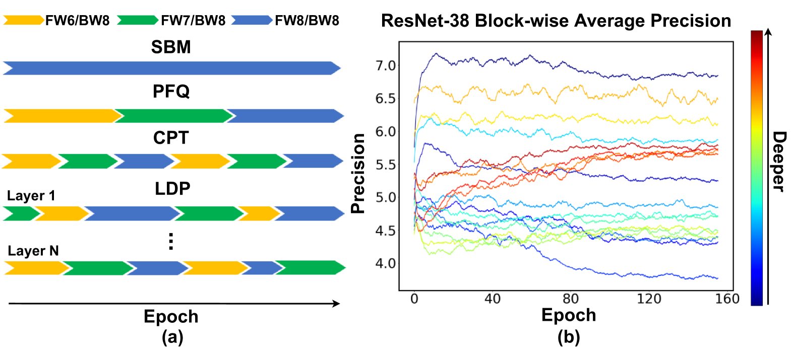
Figure 1. (a) A conceptual view of our proposed Learnable Dynamic Precision DNN training framework vs. (1) static low precision training (SBM (Banner et al., 2018)), (2) dynamic low precision training, (PFQ (Fu et al., 2020) and (3) CPT (Fu et al., 2021)). Here, each row shows the precision schedule for the whole model of the baselines, where LDP adopts a learned layer-wise dynamic precision schedule to optimally balance the training efficiency and accuracy trade-off; and (b) LDP’s learned spatial precision distribution and temporal precision schedule for ResNet-38@CIFAR-100, where different curves correspond to spatial precision distributions of different residual blocks andthe fractional precision is due to the block-wise average and moving average among iterations for better visualization.

While various low precision training techniques have been proposed to boost DNNs’ training efficiency (Banner et al., 2018; Zhou et al., 2016; Yang et al., 2020; Sun et al., 2019), most of these techniques adopt a fixed precision allocation strategy throughout the whole training process, leaving a large room for further squeezing out bit-wise savings. Motivated by the recent pioneering works, which advocate that (1) different DNN layers behave differently through the training process (Zhang et al., 2019; Veit et al., 2016) and (2) different DNN training stages favor different training schemes (Smith, 2017), a few pioneering works (Fu et al., 2020; Rajagopal et al., 2020; Fu et al., 2021) have proposed to adopt dynamic training precision, which varies the precision spatially (e.g., layer-wise precision allocation) and temporally (e.g., different precision in different training epochs) and shows promising training efficiency and optimality over their static counterparts. However, existing dynamic low precision training methods rely on manually designed dynamic precision schedules (Fu et al., 2020; Rajagopal et al., 2020; Fu et al., 2021), thus making it challenging to be directly applied to new models/tasks and limiting their achievable training efficiency.

Inspired by prior arts and motivated by their limitations, we target a general dynamic DNN training scheme without the necessity of manual fine-tuning and make the following contributions:

• We propose LDP, a Learnable Dynamic Precision (LDP) training framework to automatically learn to spatially and temporally allocate the computational cost during training by assigning different precision to different layers in each iteration, boosting the efficiency-accuracy trade-offs for both training and inference.

• To enable an end-to-end training scheme of our LDP, we propose to update the layer-wise precision in a differentiable manner by using a learnable quantization step, thus our LDP can jointly learn the layer-wise precision along with the model weights through the training process.

• Extensive experiments and ablation studies on seven networks, five datasets, and three tasks validate that LDP consistently achieves better efficiency-accuracy trade-offs over state-of-the-art (SOTA) low precision training methods for both training and inference. Specifically, compared with the best SOTA baseline, LDP achieves a 0.31% higher accuracy with a 39.1% FLOPs reduction during training, when training ResNet-20 on CIFAR-10; and the LDP trained ResNet-74 directly leads to a 49.8% reduced cost during inference.

2. Related Works

DNN quantization. DNN quantization (Wu et al., 2018; Han et al., 2015; Zhang et al., 2018; Faraone et al., 2018; Yu et al., 2020; Zhou et al., 2017; Choi et al., 2018; Banner et al., 2018; Zhou et al., 2016) is a popular DNN compression technique that aims to reduce the complexity of DNNs from the finest bit-level for achieving better efficiency-performance trade-offs. Most existing works adopt a fixed precision for all layers (Zhou et al., 2017; Faraone et al., 2018; Choi et al., 2018; Elthakeb et al., 2020). Considering the layer-wise difference in DNNs, (Wang et al., 2019; Elthakeb et al., 2020; Song et al., 2020) assign different precisions for different layers during inference, leading to better efficiency-performance trade-offs. Despite the recent trend in mixed-precision DNNs, it is still underexplored regarding how to determine the layer-wise precision in each iteration during training. It is computationally prohibitive to do so in each iteration by adopting expensive search space exploration methods like (Wang et al., 2019) did for inference. LDP tackles this via jointly learning the layer-wise precision and model weights to automatically determine the best training precision allocation in each iteration.

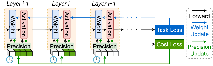
Figure 2. The proposed LDP training framework for DNNs.

Low precision training. Pioneering works (Banner et al., 2018; Yang et al., 2020; Zhou et al., 2016; Sun et al., 2019; Gupta et al., 2015) have shown that DNNs can be trained with a reduced precision without accuracy degradation. There are two major motivating applications for low precision training: (1) reducing communication cost instead of computational cost in distributed learning (Wen et al., 2017; Bernstein et al., 2018); and (2) efficient on-device/centralized learning, e.g., (Banner et al., 2018; Zhou et al., 2016; Sun et al., 2019) use a reduced precision to achieve a comparable accuracy at reduced training costs. However, most existing methods adopt a pre-defined fixed precision for all layers through the training process. Given the difference among DNN layers (Zhang et al., 2019), those methods lack the flexibility of selecting the optimal precision patterns for different layers during different training stages. A few pioneering works (Wang et al., 2020) develops a sign prediction for low-cost, low-precision back-propagation during DNN training,  (Fu et al., 2020; Rajagopal et al., 2020) propose to gradually vary the precision during training, and (Fu et al., 2021) proposes the cyclical precision training, which yet requires manually designed dynamic precision schedules. In contrast, LDP can automatically learn a dynamic precision schedule both temporally in each iteration and spatially for each layer during training without the need for manual tuning.

Dynamic precision DNNs. Dynamic precision DNNs have mostly been discussed for efficient inference (Wang et al., 2020; Shen et al., 2020). They aim to dynamically allocate the precision throughout a DNN to achieve a higher inference efficiency, which often come with a higher training cost. For example, (Shen et al., 2020) proposes to use a gating function to adapt the layer-wise precision in an input dependent manner, while (Yang and Jin, 2020) proposes to use linear interpolation to learn a fractional precision of each layer/filter; and (Zhuang et al., 2018) proposes to start from a pretrained DNN and then gradually decrease the model precision to the target one. All these methods incur additional training costs. In parallel, techniques that achieve both efficient training and inference are highly desired, motivating our LDP framework.

3. The Proposed LDP Framework

Table 1. The test accuracy of ResNet-38 trained on CIFAR-100 with different layer-wise precision schedules through the training process. In each training stage, $[a,b,c]$ represents assigning $a$-bit, $b$-bit, and $c$-bit to ResNet-38’s first three blocks, respectively.

Training Stages				Savings over static (%)	Accuracy/%
$[0\text{-th,}30\text{-th}]$	$[30\text{-th,}60\text{-th}]$	$[60\text{-th,}90\text{-th}]$	$[90\text{-th,}160\text{-th}]$
$[4,6,8]$	$[6,8,4]$	$[8,4,6]$	$[8,8,8]$	$1.10\times 10^{8}$	$68.88\pm 0.21$
$[6,8,4]$	$[8,4,6]$	$[4,6,8]$	$[8,8,8]$	$1.10\times 10^{8}$	$69.63\pm 0.14$
$[8,4,6]$	$[4,6,8]$	$[6,8,4]$	$[8,8,8]$	$1.10\times 10^{8}$	$69.36\pm 0.16$

Table 2. The test accuracy of ResNet-38 on CIFAR-100 with different frequencies for random precision change.

$k$	1	10	100	Static
Accuracy/%	$68.27\pm 0.32$	$69.71\pm 0.26$	$69.40\pm 0.24$	$69.62\pm 0.10$
Training Cost/	$1.10\times 10^{8}$	$1.10\times 10^{8}$	$1.07\times 10^{8}$	$1.32\times 10^{8}$
GBitOPs

In this section, we first present the motivation and hypothesis inspiring our development of the LDP framework, and then describe LDP’s design details.

3.1. Motivating Observations

Key insights: The optimal layer-wise precision distribution varies in different training stages and it is challenging to determine the optimal spatial/temporal precision allocation strategy on-the-fly of training. Existing works show that different DNN layers have different levels of sensitivity during training (Zhang et al., 2019) and different parts of DNNs respond differently to the same inputs (Veit et al., 2016; Greff et al., 2016; Wang et al., 2020), suggesting that dynamic precision training can boost training efficiency without hurting the accuracy. Meanwhile, (Fu et al., 2021) discovers that precision has a similar effect as the learning rate during training, providing a new angle to control the training process. These findings suggest that different DNN layers require different precision schedules during training. Therefore, identifying the optimal precision allocation can further optimize the efficiency-accuracy trade-offs. However, it is challenging to decide the best spatial/temporal precision allocation strategy during training due to the huge search space as shown in the following experiments.

Table 3. The test accuracy, computational cost, and trained models’ inference cost of ResNet-20/38/74 on CIFAR-10/100.

Datasets			CIFAR-100			CIFAR-10
Model	Method	Precision	Acc(%)	Training Cost(GBitOps)	Inference Cost(GBitOps)	Acc(%)	Training Cost(GBitOps)	Inference Cost(GBitOps)
ResNet-20	SBM	FW8/BW8	67.24	0.62e8	1.31	91.86	0.62e8	1.31
	PFQ	FW3-8/BW8	67.31	0.50e8	1.31	91.75	0.50e8	1.31
	LDP	FW3-8/BW8	67.88	0.41e8	0.71	92.08	0.41e8	0.70
	Improv.		+0.57	-18.0%	-45.8%	+0.22	-33.9%	-46.6%
	SBM	FW8/BW8	67.24	0.62e8	1.31	91.86	0.62e8	1.31
	PFQ	FW4-8/BW8	67.47	0.51e8	1.31	91.66	0.50e8	1.31
	LDP	FW4-8/BW8	67.64	0.41e8	0.66	91.86	0.41e8	0.70
	Improv.		+0.17	-19.6%	-49.6%	+0.00	-33.9%	-46.6%
ResNet-38	SBM	FW8/BW8	69.38	1.33e8	2.69	92.69	1.33e8	2.69
	PFQ	FW3-8/BW8	69.50	1.04e8	2.69	92.55	1.05e8	2.69
	LDP	FW3-8/BW8	69.77	0.87e8	1.35	92.73	0.86e8	1.36
	Improv.		+0.27	-16.3%	-49.8%	+0.04	-35.3%	-49.4%
	SBM	FW8/BW8	69.38	1.33e8	2.69	92.69	1.33e8	2.69
	PFQ	FW4-8/BW8	69.72	1.07e8	2.69	92.70	1.08e8	2.69
	LDP	FW4-8/BW8	69.81	0.87e8	1.33	92.69	0.86e8	1.37
	Improv.		+0.09	-18.7%	-50.6%	-0.01	-20.4%	-49.1%
ResNet-74	SBM	FW8/BW8	71.05	2.67e8	5.42	93.30	2.67e8	5.42
	PFQ	FW3-8/BW8	71.07	2.03e8	5.42	92.74	2.11e8	5.42
	LDP	FW3-8/BW8	71.28	1.72e8	2.83	93.63	1.72e8	2.82
	Improv.		+0.21	-15.3%	-47.8%	+0.33	-35.6%	-48.0%
	SBM	FW8/BW8	71.05	2.67e8	5.42	93.30	2.67e8	5.42
	PFQ	FW4-8/BW8	71.15	2.16e8	5.42	93.45	2.21e8	5.42
	LDP	FW4-8/BW8	71.21	1.72e8	2.78	93.50	1.73e8	2.80
	Improv.		+0.06	-20.4%	-48.7%	-0.05	-21.7%	-48.3%

Preliminary quantitative evaluation. Settings: We conduct two experiments to (1) evaluate the impact of layer-wise precision schedules in Table 1, and (2) evaluate how the precision change frequency affects the trained DNN’s accuracy in Table 2. We train ResNet-38 on CIFAR-100 for 160 epochs following the training setting in (Wang et al., 2018) for both experiments. Specifically, in Table 1, we divide the training into four stages: [0-th, 30-th], [30-th, 60-th], [60-th, 90-th], and [90-th, 160-th], and assign different precisions to different blocks of ResNet-38 in the first three training stages and adopt a static 8-bit low precision in the last training stage, in order to evaluate the impact of assigning different precisions to different layers during training under the same total training budget of GBitOPs (Gigabit operations). In Table 2, we randomly assign a precision value from $[4,6,8]$-bit to all layers of the DNNs every $k$ iterations to quantize the DNN weights, activations, and gradients in the first 90 training epochs. In this experiment, we evaluate results with different $k$ values in $[1,10,100]$. We report the average accuracy and the standard deviation of three runs for all experiments above.

Results: We observe that (1) in Table 1, different precision schedules through the training process vary the final accuracy by as high as $0.75\%$ under the same total training cost; and (2) in Table 2, the best precision change frequency leads to (1) as high as a $1.44\%$ higher accuracy over other frequencies and (2) a $0.09\%$ higher accuracy with a $16\%$ lower training cost than the static precision training baseline.

Analysis: This set of experiments shows that (1) given the same total training cost budget, how to allocate the training cost budget by spatially and temporally scheduling the training precision during training can significantly impact the finally achieved model accuracy; (2) the precision changing frequency also affects the achieved accuracy and even a naive randomly generated precision schedule with an adequately selected precision changing frequency can offer a better training efficiency; and (3) there exists no golden rule for determining the optimal spatial/temporal precision schedule, which highly relies on manual hyper-parameter tuning in SOTA methods (Fu et al., 2020; Rajagopal et al., 2020; Fu et al., 2021), and it is challenging to automatically derive the optimal spatial/temporal schedule of training precision given the huge space of layer-wise precision schedule.

3.2. The Proposed LDP Framework

Existing mixed-precision networks rely on costly trial-and-error methods (e.g., reinforcement learning-based (Wang et al., 2019) and evolutionary-based (Yuan et al., 2020) ones) to determine the layer-wise precision. It is thus computationally impractical to apply these methods in each training iteration. Therefore, we propose to make the precision be aware of training states via jointly learning the layer-wise precision with the model weights in a differentiable manner.

As the precision itself is discrete and non-differentiable to the loss function, we introduce a continuous layer-wise learnable parameter $\beta^{l}$ for each layer $l$ with a quantization step size $s^{l}$ defined as:

(1) $$s^{l}=\frac{R_{range}}{2^{\text{Round}(\beta^{l}\times N)}-1},$$

where $R_{range}$ is the dynamic range of input parameters, $N$ is the range of the available precision, and Round$(.)$ indicates rounding the value to the nearest integer. Given a full precision value $I$ at layer $l$, its quantized counterpart $Q$ with $s^{l}$ can be defined as:

(2) $$Q=\text{Round}(\frac{I-I_{ZeroPoint}}{s^{l}})+I_{ZeroPoint},$$

where $I_{ZeroPoint}$ is an input-dependent parameter for normalizing the inputs. In this way, $\beta^{l}$ can be integrated into DNNs’ computational flow and updated with respect to the loss function in a differentiable manner.

Loss function. As a higher precision favors more precise gradients and thus increased accuracy, directly updating the aforementioned $\beta^{l}$ in each layer $l$ with respect to the task loss $L_{task}$ only leads to a monotony increase of $\beta^{l}$ and thus a higher training cost. This conflicts with the goal of LDP, which is to learn a layer-wise dynamic precision schedule to better allocate the training cost within the network and during the training process. To address this discrepancy, we incorporate a cost loss $L_{cost}$ into the network’s loss function to control the trade-off balance between model efficiency and accuracy, where $L_{cost}$ is defined as:

(3) $$L_{cost}=\left\{\begin{array}[]{lr}0,&\text{if }C<T\\ C,&\text{if }C\geq T\\ \end{array}\right.$$

where $T$ is the target iteration-wise training cost and $C$ is the forward pass cost in the current iteration defined as:

(4) $$C=\sum_{l=1}^{L}O^{l}\times\frac{\text{Round}(\beta^{l}\times N)}{32}^{2},$$

where $O^{l}$ is the required BitOPs for a full precision forward pass of layer $l$. However, the scale of $L_{task}$ and $L_{cost}$ can vary significantly throughout the training process and thus may require a tedious finetuning process to balance these two loss terms when applying LDP to different tasks. Thus, we adopt a balance factor $\alpha$ to balance the gradient of each layer’s $\beta^{l}$ with respect to $L_{task}$ and $L_{cost}$. Specifically, the overall precision gradients $G^{l}$ for layer $l$ is defined as:

(5) $$\vspace{0.2em}G^{l}=G^{l}_{T}+\alpha\times G^{l}_{C}\times\frac{\text{Mean}(\text{Abs}(G_{T}))}{\text{Mean}(\text{Abs}(G_{C}))+\epsilon},\vspace{0.4em}$$

where $\text{Mean}(\text{Abs}(G_{T}))$ and $\text{Mean}(\text{Abs}(G_{C}))$ are the network-wise averaged absolute values for the precision gradients with respect to $L_{task}$ and $L_{cost}$, respectively, and $\epsilon$ is a small term to guarantee the training stability. To effectively prevent the precision from further growth, it is intuitive to constrain the contribution of $L_{task}$ and $L_{cost}$ to $G^{l}$ to the same scale, so we set $\alpha=1$ in our implementation. In this way, when the precision is too high and the target training budget per iteration is exceeded, the cost term can effectively prevent the further increase in training precision without severely reducing the overall model precision, avoiding unrecoverable performance degradation. It is worth noting that although we calculate the gradient separately, it does not introduce additional computation costs. This is because $G^{l}_{C}$ can be naturally acquired once the network structure is fixed and does not need to specifically run backpropagation with respect to $L_{cost}$.

Potential hardware supports for LDP. Scalable-precision architectures have been extensively studied (Sharma et al., 2018; Judd et al., 2016; Lee et al., 2018) to support adaptive-precision execution of DNNs, i.e., select different precisions for different layers/iterations. In addition, it is promising to deploy LDP on other mixed-precision DNN accelerators (Lee et al., 2019; Kim et al., 2020).

4. Experiments

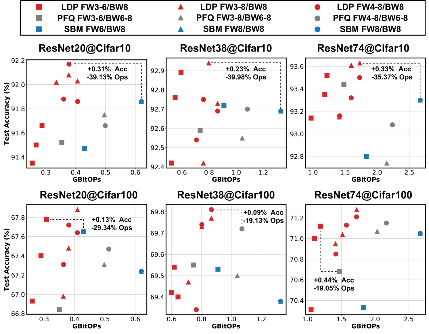
Figure 3. Benchmarking LDP with the SOTA static low precision training method SBM and dynamic precision training method PFQ in terms of model accuracy and training cost on ResNet-20/38/74 and CIFAR10/100.

4.1. Experiment Setup

Models, datasets, and baselines. We evaluate our method on seven models (including four ResNet-based models (He et al., 2016), Vision Transformer (Touvron et al., 2021), Transformer (Vaswani et al., 2017) and an efficient super-resolution model, PAN (Zhao et al., 2020)) and five datasets across three tasks (including image classification on CIFAR-10/100 (Krizhevsky et al., 2009), ImageNet (Deng et al., 2009), image super-resolution (SR) trained on DIV2K (Agustsson and Timofte, 2017) and Flickr2K (Timofte et al., 2017) and evaluated on Urban-100 (Yang et al., 2010), and language modeling on WikiText-103 (Merity et al., 2017)). Baselines: We benchmark the proposed LDP over SOTA low precision training methods, including PFQ (Fu et al., 2020), CPT (Fu et al., 2021), and SBM (Banner et al., 2018). For a fair comparison, we use the quantizer proposed in SBM (Banner et al., 2018) for all our baselines.

Training settings. We follow the standard training setting in all experiments, i.e., (Wang et al., 2018) and (He et al., 2016) for CIFAR-10/100 and ImageNet, respectively, (Zhao et al., 2020) for SR and (Baevski and Auli, 2018) for language modeling. Unless specifically specified, we use a learning rate of 0.1 and an SGD optimizer for learning the precision, i.e., $\beta^{l}$ in Eq. 1, and we set $T$ as $60\%$ of the iteration-wise training cost $T_{stat}$ of the static low precision training baseline. For LDP, the training precision setting FW3-8/BW8 means the range of the learnable precision is 3$\sim$8-bit and the gradient is quantized to 8-bit; for PFQ and CPT, we follow the definition in their original paper (Fu et al., 2020; Fu et al., 2021).

4.2. Benchmark with SOTA Low Precision Training Methods

Benchmark on CIFAR-10/100. We first benchmark LDP with two SOTA low precision training methods: (1) the static low precision training method SBM (Banner et al., 2018), and (2) the dynamic low precision training method PFQ (Fu et al., 2020) on three different networks, i.e., ResNet-20/38/74, under two different precision schemes, i.e., FW3-8/BW8 and FW4-8/BW8 on CIFAR-10/100 datasets. The results are shown in Table 3, where results with the highest accuracy are marked in bold. The accuracy improvement and training/inference cost reduction is the difference between LDP and the strongest baseline with the highest accuracy under the same settings. From Table 3, we have the following observations: (1) LDP consistently achieves better accuracy-training efficiency trade-offs than all baseline methods. Specifically, with $20.4\%\sim 39.6\%$ less training cost, LDP can achieve a comparable or even better accuracy ($-0.16\%\sim+0.56\%$) on CIFAR-10 and CIFAR-100 datasets; (2) LDP’s learned precision naturally boosts the inference efficiency, reducing the inference cost by $29.0\%\sim 68.3\%$ compared with models trained with SBM or PFQ.

To further evaluate the overall performance of LDP, we evaluate LDP’s performance under different $T\in[0.5T_{stat},0.7T_{stat}]$. The results are shown in Fig. 3 and we can observe that: (1) the training cost can be effectively controlled by the value of $T$, indicating the easiness to fit LDP onto different training tasks with varied training budgets, and (2) LDP keeps achieving the best accuracy-efficiency trade-off under different training cost budgets.

Table 4. The test accuracy, training cost, and trained models’ inference cost of ResNet-18 and DeiT-Tiny on ImageNet.

Model	Method	Precision	Acc(%)	Training Cost	Inference Cost
				(GBitOps)	(GBitOps)
ResNet-18	SBM	FW8/BW8	69.60	2.86e9	1.46e1
	CPT	FW4-8/BW8	69.64	1.99e9	1.46e1
	PFQ	FW4-8/BW6-8	69.12	2.47e9	1.46e1
	LDP	FW4-8/BW8	69.62	1.83e9	1.01e1
	Improv.		-0.02	-8.1%	-30.8%
DeiT-Tiny	SBM	FW8/BW8	71.71	4.74e9	0.96e1
	CPT	FW4-8/BW8	71.84	3.29e9	0.96e1
	PFQ	FW4-8/BW6-8	71.70	3.96e9	0.96e1
	LDP	FW4-8/BW8	71.92	3.08e9	0.67e1
	Improv.		+0.08	-6.4%	-30.2%

Benchmark on ImageNet. We further verify the scalability of LDP on the more challenging ImageNet dataset across different model architectures. As shown in Table 4, LDP still achieves comparable accuracy with less training cost compared with the most competitive baseline methods. Specifically, compared with CPT, LDP achieves a $0.08\%$ higher accuracy with $10.6\%$ less training cost to train DeiT-Tiny under FW3-8/BW8. Moreover, the LDP trained models are still more efficient than models trained with other baseline methods with an improvement in inference efficiency ranging between $11.0\%\sim 35.2\%$.

Table 5. The PSNR and inference cost of PAN on Urban-100.

Method	Precision	Urban-100	Inference Cost
			(GBitOps)
Half-Precision	FW16/BW16	26.01	6.43e1
PFQ	FW8-16/BW16	25.99	6.43e1
CPT	FW8-16/BW16	26.01	6.43e1
LDP	FW8-16/BW16	26.03	5.22e1
Improv.		+0.02	-18.8%

Table 6. The test perplexity (the lower, the better) and training cost of Transformer on WikiText-103.

Method	Precision	Perplexity	Training Cost (GBitOps)
SBM	FW8/BW8	31.77	9.87e5
LDP	FW4-8/BW8	30.81	7.31e5
Improv.		-0.96	-25.9%

Benchmark on SR task. We also evaluate LDP on the SR task. It is noteworthy that given the nature of the relatively smaller gradient of the SR task, it is non-trivial to train the SR models with reduced precision. We only quantize the feature extraction part in PAN with a precision scheme of FW8-16/BW16 and a precision learning rate of $20$ and $T=0.85T_{stat}$. The results are shown in Table 5 that LDP achieves a 0.02dB higher peak signal-to-noise ratio (PSNR) with $18.8\%$ less inference cost on Urban-100 compared with the original half-precision training, showing LDP’s ability in further boosting models performance.

Benchmark on natural language processing (NLP) task. To validate the general effectiveness of LDP on NLP tasks, we also apply LDP on a language modeling task WikiText-103 (Merity et al., 2017) on top of the Transformer (Vaswani et al., 2017) model. As shown in Table 6, LDP consistently achieves better performance than the SBM baseline with less training and inference cost, showing that the proposed LDP can be a general technique among different tasks.

Ablation study about the choice of $\alpha$. To evaluate LDP’s sensitivity to $\alpha$, we apply LDP on ResNet-20/38 with different values of $\alpha$. As shown in Table 7, different values of $\alpha$ do not have a significant impact on the achieved accuracy ($<0.2\%$ accuracy variance), suggesting the easiness of deploying LDP without the need for exhaustive hyperparameters finetuning.

4.3. Visualization of LDP’s Learned Precision

We visualize the temporal and spatial precision distribution learned by LDP to understand the characteristics of different models’ learning process and the redundancy of different modules.

Table 7. Training ResNet-20/38 on CIFAR-100 with different $\alpha$ using FW3-8/BW8.

	$\alpha=1.5$		$\alpha=1$		$\alpha=0.5$
	Acc (%)	GBitOps	Acc (%)	GBitOps	Acc (%)	GBitOps
ResNet-20	66.98	0.39e8	67.08	0.41e8	67.13	0.53e8
ResNet-38	69.85	0.76e8	70.06	0.80e8	69.94	1.14e8

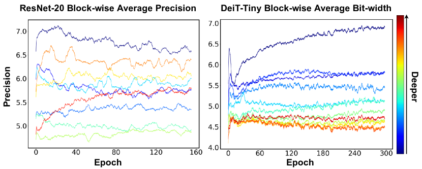
Figure 4. Visualization of spatial precision distribution and temporal precision schedule during training. The warmer the line is, the deeper the corresponding layer is in the model.

Temporary precision distribution during training. We first visualize the learned precision schedule of ResNet-20@CIFAR-100 and DeiT-Tiny@ImageNet through the training process. As shown in Fig. 4, there are three patterns in the learned precision schedule of ResNet-20: (1) For shallower layers, the block-wise average precision first rapidly grows to high precision in the initial iterations of training, then gradually decrease, (2) for layers in the middle of the model, the precision keeps high through the whole training process, and (3) for deeper layers, the precision would gradually increase along with the training process.

Such learned precision schedule aligns with the understanding of ResNet’s learning process (Achille et al., 2018), where high precision in shallow layers helps to learn the low-level information in the initial training stage; while at a later training stage, shallow layers’ learned features can be represented in low precision and higher precision in deeper layers help better abstract semantic information from the low-level features passed from shallower layers.

On the other hand, the precision schedule in the DeiT-Tiny model is pretty different from that of ResNet-20 due to the difference in the model structure, leading to higher difficulty for training, as suggested in (Touvron et al., 2021; Steiner et al., 2021). We notice the precision schedule of all blocks keeps growing to certain block-specific values. Such gradually increased spatial precision distribution echos the DeiT block-wise redundancy analyzed in (Zhou et al., 2021).

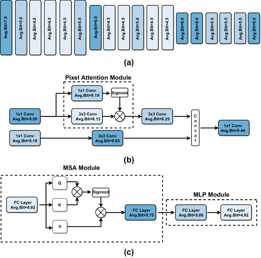
Figure 5. Spatial precision distribution of models where deeper color indicates a higher precision. (a) Block-wise average precision of ResNet-38, layer-wise average precision of (b) PAN’s SCPA module, and (c) DeiT-Tiny’s blocks.

Learned spatial precision distribution. We further investigate the learned spatial precision distribution on ResNet-38 (Fig. 5(a)), PAN (Fig. 5(b)) and DeiT-Tiny (Fig. 5(c)), respectively.

In ResNet-38, LDP learns (1) significantly higher precisions in blocks containing downsampling layers, and (2) higher precision in the deep blocks with the lowest resolution, indicating less redundancy in these blocks which aligns with the observations in (Wang et al., 2020; Shen et al., 2020).

In the SCPA module in PAN, we observe that in the two-stream architecture, there exists a layer with relatively high precision in each branch of PA, suggesting that it is critical to preserve the detail of information in each branch.

We further visualize the DeiT block’s spatial precision distribution and observe that the sequentially connected fully-connected (FC) layers have a gradually decreased precision, indicating the redundancy in the stacked FC layers. This motivates the necessity of reducing the redundancy in such layers, aligning with the observations in (Guo et al., 2021; Park and Kim, 2022).

5. Conclusion

In this paper, we propose a Learnable Dynamic Precision training framework called LDP for efficient and effective low precision training. By adding a learnable precision parameter, LDP can automatically learn a spatial precision distribution and a temporal precision schedule for each iteration on-the-fly during the training process. Extensive experiments, ablation studies, and visualizations verify that LDP can learn an effective precision schedule spatially and temporarily, pushing forward the frontier of the trade-off between task performances and training cost.

References

- (1)
- Achille et al. (2018) Alessandro Achille, Matteo Rovere, and Stefano Soatto. 2018. Critical learning periods in deep networks. In International Conference on Learning Representations.
- Agustsson and Timofte (2017) Eirikur Agustsson and Radu Timofte. 2017. Ntire 2017 challenge on single image super-resolution: Dataset and study. In Proceedings of the IEEE conference on computer vision and pattern recognition workshops. 126–135.
- Baevski and Auli (2018) Alexei Baevski and Michael Auli. 2018. Adaptive input representations for neural language modeling. arXiv preprint arXiv:1809.10853 (2018).
- Banner et al. (2018) Ron Banner, Itay Hubara, Elad Hoffer, and Daniel Soudry. 2018. Scalable methods for 8-bit training of neural networks. arXiv preprint arXiv:1805.11046 (2018).
- Bernstein et al. (2018) Jeremy Bernstein, Yu-Xiang Wang, Kamyar Azizzadenesheli, and Animashree Anandkumar. 2018. signSGD: Compressed optimisation for non-convex problems. In International Conference on Machine Learning. PMLR, 560–569.
- Choi et al. (2018) Jungwook Choi, Zhuo Wang, Swagath Venkataramani, Pierce I-Jen Chuang, Vijayalakshmi Srinivasan, and Kailash Gopalakrishnan. 2018. Pact: Parameterized clipping activation for quantized neural networks. arXiv preprint arXiv:1805.06085 (2018).
- Deng et al. (2009) Jia Deng, Wei Dong, Richard Socher, Li-Jia Li, Kai Li, and Li Fei-Fei. 2009. Imagenet: A large-scale hierarchical image database. In 2009 IEEE conference on computer vision and pattern recognition. Ieee, 248–255.
- Elthakeb et al. (2020) Ahmed T Elthakeb, Prannoy Pilligundla, Fatemehsadat Mireshghallah, Amir Yazdanbakhsh, and Hadi Esmaeilzadeh. 2020. ReLeQ: A Reinforcement Learning Approach for Automatic Deep Quantization of Neural Networks. IEEE Micro 40, 5 (2020), 37–45.
- Faraone et al. (2018) Julian Faraone, Nicholas Fraser, Michaela Blott, and Philip HW Leong. 2018. Syq: Learning symmetric quantization for efficient deep neural networks. In Proceedings of the IEEE Conference on Computer Vision and Pattern Recognition. 4300–4309.
- Fu et al. (2021) Yonggan Fu, Han Guo, Meng Li, Xin Yang, Yining Ding, Vikas Chandra, and Yingyan Lin. 2021. CPT: Efficient Deep Neural Network Training via Cyclic Precision. arXiv preprint arXiv:2101.09868 (2021).
- Fu et al. (2020) Yonggan Fu, Haoran You, Yang Zhao, Yue Wang, Chaojian Li, Kailash Gopalakrishnan, Zhangyang Wang, and Yingyan Lin. 2020. Fractrain: Fractionally squeezing bit savings both temporally and spatially for efficient dnn training. arXiv preprint arXiv:2012.13113 (2020).
- Greff et al. (2016) Klaus Greff, Rupesh K Srivastava, and Jürgen Schmidhuber. 2016. Highway and residual networks learn unrolled iterative estimation. arXiv preprint arXiv:1612.07771 (2016).
- Guo et al. (2021) Jianyuan Guo, Kai Han, Han Wu, Chang Xu, Yehui Tang, Chunjing Xu, and Yunhe Wang. 2021. Cmt: Convolutional neural networks meet vision transformers. arXiv preprint arXiv:2107.06263 (2021).
- Gupta et al. (2015) Suyog Gupta, Ankur Agrawal, Kailash Gopalakrishnan, and Pritish Narayanan. 2015. Deep learning with limited numerical precision. In International conference on machine learning. PMLR, 1737–1746.
- Han et al. (2015) Song Han, Huizi Mao, and William J Dally. 2015. Deep compression: Compressing deep neural networks with pruning, trained quantization and huffman coding. arXiv preprint arXiv:1510.00149 (2015).
- He et al. (2016) K. He et al. 2016. Deep residual learning for image recognition. In CVPR. 770–778.
- Judd et al. (2016) Patrick Judd, Jorge Albericio, Tayler Hetherington, Tor M Aamodt, and Andreas Moshovos. 2016. Stripes: Bit-serial deep neural network computing. In 2016 49th Annual IEEE/ACM International Symposium on Microarchitecture (MICRO). IEEE, 1–12.
- Kim et al. (2020) Chang Hyeon Kim, Jin Mook Lee, Sang Hoon Kang, Sang Yeob Kim, Dong Seok Im, and Hoi Jun Yoo. 2020. 1b-16b variable bit precision dnn processor for emotional hri system in mobile devices. Journal of Integrated Circuits and Systems 6, 3 (2020).
- Krizhevsky et al. (2009) Alex Krizhevsky, Geoffrey Hinton, et al. 2009. Learning multiple layers of features from tiny images. (2009).
- Lee et al. (2018) Jinmook Lee, Changhyeon Kim, Sanghoon Kang, Dongjoo Shin, Sangyeob Kim, and Hoi-Jun Yoo. 2018. UNPU: An energy-efficient deep neural network accelerator with fully variable weight bit precision. IEEE Journal of Solid-State Circuits 54, 1 (2018), 173–185.
- Lee et al. (2019) Jinsu Lee, Juhyoung Lee, Donghyeon Han, Jinmook Lee, Gwangtae Park, and Hoi-Jun Yoo. 2019. 7.7 LNPU: A 25.3 TFLOPS/W sparse deep-neural-network learning processor with fine-grained mixed precision of FP8-FP16. In 2019 IEEE International Solid-State Circuits Conference-(ISSCC). IEEE, 142–144.
- Merity et al. (2017) Stephen Merity, Nitish Shirish Keskar, and Richard Socher. 2017. Regularizing and optimizing LSTM language models. arXiv preprint arXiv:1708.02182 (2017).
- Park and Kim (2022) Namuk Park and Songkuk Kim. 2022. How Do Vision Transformers Work? arXiv preprint arXiv:2202.06709 (2022).
- Rajagopal et al. (2020) Aditya Rajagopal, Diederik Vink, Stylianos Venieris, and Christos-Savvas Bouganis. 2020. Multi-Precision Policy Enforced Training (MuPPET): A precision-switching strategy for quantised fixed-point training of CNNs. In International Conference on Machine Learning. PMLR, 7943–7952.
- Sharma et al. (2018) Hardik Sharma, Jongse Park, Naveen Suda, Liangzhen Lai, Benson Chau, Vikas Chandra, and Hadi Esmaeilzadeh. 2018. Bit fusion: Bit-level dynamically composable architecture for accelerating deep neural network. In 2018 ACM/IEEE 45th Annual International Symposium on Computer Architecture (ISCA). IEEE, 764–775.
- Shen et al. (2020) Jianghao Shen, Yue Wang, Pengfei Xu, Yonggan Fu, Zhangyang Wang, and Yingyan Lin. 2020. Fractional skipping: Towards finer-grained dynamic cnn inference. In Proceedings of the AAAI Conference on Artificial Intelligence, Vol. 34. 5700–5708.
- Smith (2017) Leslie N Smith. 2017. Cyclical learning rates for training neural networks. In 2017 IEEE winter conference on applications of computer vision (WACV). IEEE, 464–472.
- Song et al. (2020) Zhuoran Song, Bangqi Fu, Feiyang Wu, Zhaoming Jiang, Li Jiang, Naifeng Jing, and Xiaoyao Liang. 2020. DRQ: dynamic region-based quantization for deep neural network acceleration. In 2020 ACM/IEEE 47th Annual International Symposium on Computer Architecture (ISCA). IEEE, 1010–1021.
- Steiner et al. (2021) Andreas Steiner, Alexander Kolesnikov, Xiaohua Zhai, Ross Wightman, Jakob Uszkoreit, and Lucas Beyer. 2021. How to train your ViT? Data, Augmentation, and Regularization in Vision Transformers. arXiv preprint arXiv:2106.10270 (2021).
- Sun et al. (2019) Xiao Sun, Jungwook Choi, Chia-Yu Chen, Naigang Wang, Swagath Venkataramani, Vijayalakshmi Viji Srinivasan, Xiaodong Cui, Wei Zhang, and Kailash Gopalakrishnan. 2019. Hybrid 8-bit floating point (HFP8) training and inference for deep neural networks. Advances in neural information processing systems 32 (2019), 4900–4909.
- Timofte et al. (2017) Radu Timofte, Eirikur Agustsson, Luc Van Gool, Ming-Hsuan Yang, and Lei Zhang. 2017. Ntire 2017 challenge on single image super-resolution: Methods and results. In Proceedings of the IEEE conference on computer vision and pattern recognition workshops. 114–125.
- Touvron et al. (2021) Hugo Touvron, Matthieu Cord, Matthijs Douze, Francisco Massa, Alexandre Sablayrolles, and Hervé Jégou. 2021. Training data-efficient image transformers & distillation through attention. In International Conference on Machine Learning. PMLR, 10347–10357.
- Vaswani et al. (2017) Ashish Vaswani, Noam Shazeer, Niki Parmar, Jakob Uszkoreit, Llion Jones, Aidan N Gomez, Łukasz Kaiser, and Illia Polosukhin. 2017. Attention is all you need. In Advances in neural information processing systems. 5998–6008.
- Veit et al. (2016) Andreas Veit, Michael Wilber, and Serge Belongie. 2016. Residual networks behave like ensembles of relatively shallow networks. arXiv preprint arXiv:1605.06431 (2016).
- Wang et al. (2019) Kuan Wang, Zhijian Liu, Yujun Lin, Ji Lin, and Song Han. 2019. Haq: Hardware-aware automated quantization with mixed precision. In Proceedings of the IEEE/CVF Conference on Computer Vision and Pattern Recognition. 8612–8620.
- Wang et al. (2018) Xin Wang, Fisher Yu, Zi-Yi Dou, Trevor Darrell, and Joseph E Gonzalez. 2018. Skipnet: Learning dynamic routing in convolutional networks. In Proceedings of the European Conference on Computer Vision (ECCV). 409–424.
- Wang et al. (2020) Yue Wang, Jianghao Shen, Ting-Kuei Hu, Pengfei Xu, Tan Nguyen, Richard Baraniuk, Zhangyang Wang, and Yingyan Lin. 2020. Dual dynamic inference: Enabling more efficient, adaptive, and controllable deep inference. IEEE Journal of Selected Topics in Signal Processing 14, 4 (2020), 623–633.
- Wen et al. (2017) Wei Wen, Cong Xu, Feng Yan, Chunpeng Wu, Yandan Wang, Yiran Chen, and Hai Li. 2017. Terngrad: Ternary gradients to reduce communication in distributed deep learning. arXiv preprint arXiv:1705.07878 (2017).
- Wu et al. (2018) Junru Wu, Yue Wang, Zhenyu Wu, Zhangyang Wang, Ashok Veeraraghavan, and Yingyan Lin. 2018. Deep k-means: Re-training and parameter sharing with harder cluster assignments for compressing deep convolutions. In International Conference on Machine Learning. PMLR, 5363–5372.
- Yang et al. (2010) Jianchao Yang, John Wright, Thomas S Huang, and Yi Ma. 2010. Image super-resolution via sparse representation. IEEE transactions on image processing 19, 11 (2010), 2861–2873.
- Yang and Jin (2020) Linjie Yang and Qing Jin. 2020. FracBits: Mixed Precision Quantization via Fractional Bit-Widths. arXiv preprint arXiv:2007.02017 (2020).
- Yang et al. (2020) Yukuan Yang, Lei Deng, Shuang Wu, Tianyi Yan, Yuan Xie, and Guoqi Li. 2020. Training high-performance and large-scale deep neural networks with full 8-bit integers. Neural Networks 125 (2020), 70–82.
- Yu et al. (2020) Zhongzhi Yu, Yemin Shi, Tiejun Huang, and Yizhou Yu. 2020. Kernel Quantization for Efficient Network Compression. arXiv preprint arXiv:2003.05148 (2020).
- Yuan et al. (2020) Yong Yuan, Chen Chen, Xiyuan Hu, and Silong Peng. 2020. Evoq: Mixed precision quantization of dnns via sensitivity guided evolutionary search. In 2020 International Joint Conference on Neural Networks (IJCNN). IEEE, 1–8.
- Zhang et al. (2019) Chiyuan Zhang, Samy Bengio, and Yoram Singer. 2019. Are all layers created equal? arXiv preprint arXiv:1902.01996 (2019).
- Zhang et al. (2018) Dongqing Zhang, Jiaolong Yang, Dongqiangzi Ye, and Gang Hua. 2018. Lq-nets: Learned quantization for highly accurate and compact deep neural networks. In Proceedings of the European conference on computer vision (ECCV). 365–382.
- Zhao et al. (2020) Hengyuan Zhao, Xiangtao Kong, Jingwen He, Yu Qiao, and Chao Dong. 2020. Efficient image super-resolution using pixel attention. In European Conference on Computer Vision. Springer, 56–72.
- Zhou et al. (2017) Aojun Zhou, Anbang Yao, Yiwen Guo, Lin Xu, and Yurong Chen. 2017. Incremental network quantization: Towards lossless cnns with low-precision weights. arXiv preprint arXiv:1702.03044 (2017).
- Zhou et al. (2021) Daquan Zhou, Bingyi Kang, Xiaojie Jin, Linjie Yang, Xiaochen Lian, Zihang Jiang, Qibin Hou, and Jiashi Feng. 2021. Deepvit: Towards deeper vision transformer. arXiv preprint arXiv:2103.11886 (2021).
- Zhou et al. (2016) Shuchang Zhou, Yuxin Wu, Zekun Ni, Xinyu Zhou, He Wen, and Yuheng Zou. 2016. Dorefa-net: Training low bitwidth convolutional neural networks with low bitwidth gradients. arXiv preprint arXiv:1606.06160 (2016).
- Zhuang et al. (2018) Bohan Zhuang, Chunhua Shen, Mingkui Tan, Lingqiao Liu, and Ian Reid. 2018. Towards effective low-bitwidth convolutional neural networks. In Proceedings of the IEEE conference on computer vision and pattern recognition. 7920–7928.