Adaptive Environment Modeling Based Reinforcement Learning for Collision Avoidance in Complex Scenes

Abstract

The major challenges of collision avoidance for robot navigation in crowded scenes lie in accurate environment modeling, fast perceptions, and trustworthy motion planning policies. This paper presents a novel adaptive environment model based collision avoidance reinforcement learning (i.e., AEMCARL) framework for an unmanned robot to achieve collision-free motions in challenging navigation scenarios. The novelty of this work is threefold: (1) developing a hierarchical network of gated-recurrent-unit (GRU) for environment modeling; (2) developing an adaptive perception mechanism with an attention module; (3) developing an adaptive reward function for the reinforcement learning (RL) framework to jointly train the environment model, perception function and motion planning policy. The proposed method is tested with the Gym-Gazebo simulator and a group of robots (Husky and Turtlebot) under various crowded scenes. Both simulation and experimental results have demonstrated the superior performance of the proposed method over baseline methods.

I INTRODUCTION

End-to-end RL-based unmanned mobile robots are advantageous in the high degree of autonomy, robustness against unmodeled uncertainties, and high-speed decision [1, 2, 3]. The main components of RL-based unmanned robots include (1) sensing, motion and communication units, (2) world and robot models, (3) policy and probability based reward functions, and (4) state and action spaces. Developing RL-based autonomous robot systems for crowded scenes, as shown in Fig. 1, has to deal with the following technical challenges:

1. Dynamic environment modeling. In the real world, many objects such as pedestrians, vehicles, animals move around with various behaviors and interactions; how to develop a hierarchical model to represent such a dynamic environment in different degrees of complexity is still a challenging problem;

2. Adaptive perception mechanism. The robot should be able to perceive the environment with an attention mechanism, and adaptively use computational resources according to perception confidences.

3. Collision-free policy for motion planning. The quality of RL-based motion planning policies relies on the selection of reward functions and state representation. An ideal reward function should reduce not only the collision possibility between the robot and the nearest obstacle but also that between the robot and neighboring obstacles within a time window.

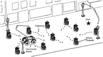
Figure 1: An illustration of an unmanned robot with the capability of collision avoidance in crowded scenes (of robotic mobile obstacles). All robots are equipped with Ultra-wideband (UWB) modules for distance measurement and localization.

Most RL-based crowd-aware approaches use simple dynamic environment models such as multi-layer perceptron (MLP), which cannot fully describe real-world complexities and uncertainties. Meanwhile, perception functions have to trade off between decision speed and environment modeling accuracy by selecting proper structures of deep learning models [4]. On the other hand, reward function and attention mechanisms [5, 4] have been developed to make better decisions with reduced computational workloads. However, no such a RL-based framework has been developed yet, which contains high-order environment models as well as adaptive perception, adaptive reward function, and attention modules.

TABLE I: A brief summary of Traditional and Reinforcement learning based collision-free navigation methods

Scheme	Navigation Method	Dynamic Environment Modeling			Adaptive Perception Mechanism			Collision-free Policy
		Agent number	Multi agent representation	Hierarchical representation	Perception confidence	Self-tuning	Attention mechanism	Reward
Traditional Approach	RVO [6]	Arbitrary	Math modeling	$\times$	$\times$	$\times$	$\times$	N/A
	ORCA [7]	Arbitrary	Math modeling	$\times$	$\times$	$\times$	$\times$	N/A
RL-based Approach	LSTM-RL [8]	Fixed Number	LSTM & MLP	$\times$	$\times$	$\times$	$\times$	+
	CADRL [9] $\setminus$ SARL [5]	Fixed Number$\setminus$High	MLP	$\times$	$\times$	$\times$	$\times\setminus\surd$	+
	RGL [4]$\setminus$G-GCNRL [10]	Fixed Number$\setminus$High	GNN$\setminus$GCN	$\times$	$\times$	$\times$	$\surd$	++$\setminus$+
	SODARL [11]	Arbitrary	CNN	$\times$	$\times$	$\times$	$\surd$	++
	AEMCARL (Ours)	Arbitrary	GRU	$\surd$	$\surd$	$\surd$	$\surd$	++

The number of + reflects the performance of this functionality of the method. Symbol $\surd$: This functionality is supported. Symbol $\times$: This functionality is not supported or not considered. CA: Collision avoidance. GNN: Graph neural network. GCN: Graph convolution network. FC: Fully connection. The angular map in SODARL plays a same role with the attention mechanism.

In this paper, we propose a robust RL-based motion planning framework with an adaptive environmental model (AEM) and adaptive reward function to achieve collision-free navigation in crowded scenarios. The estimated perception confidences are used to change the AEM structure in real-time. Adaptive reward function and attention modules are developed to improve the generalization capability of the system. The main contributions of this paper include

1. We design a novel RL-based motion planning framework, which consists of modules of modeling, attention, and action, to achieve real-time navigation with collision avoidance;

2. We propose a hierarchical environment model to represent multiple agents of dynamic environments;

3. We develop a perception confidence based adaptation mechanism as well as an attention module to achieve fast decision with reduced computational complexity;

4. We propose an adaptive reward function reward function and a set of robust navigation policy training algorithms. The open-source code is available at:
   https://github.com/SJWang2015/AEMCARL.

The rest of this paper is organized as follows. Section II introduces the related work on RL-based motion planning. Section III describes the system setup and problem statement. Section IV presents the proposed method. Section V provides the experiment results and ablation studies. Section VI concludes this paper and outlines future work.

II RELATED WORK

TABLE I summarizes a number of navigation methods with collision avoidance for a single robot in crowded scenes. Compared with conventional methods, the RL-based approaches can learn from the various simulation experiences to generate robust and high-efficiency motion planning policies. The most challenging problem for motion planning in crowded scenes is to build dynamic environment models (DEMs) which should accommodate a large number of mobile robots, and describe the spatial and temporal interactions among agents. Most DEMs can be classified into two groups: object-centric and relation-centric. The former emphasizes the pose and velocity information of agents [12]; while the latter describes the current and future relationships among agents [12]. To achieve better modeling performance, fully connected (FC) layers and long short-term memory (LSTM) [13] units have been used to describe long-term and long-range relation-centric interactions among agents [3, 14]. Compared with LSTM and GRUs [15], Transformer  [16] don’t rely on the order of input data, and can capture the relations between participants precisely. The graph networks have also been used to build the relationships of all agents in the environment [4, 10], which are flexible to combine with the attention mechanism, and help the network achieve better obstacle avoidance performance. To inference the dynamic environmental relationship in the future, the graph must be fixed, or the drastically changing number of obstacles might cause the algorithm’s performance to be unstable.

Recurrent and feedforward networks [5, 9] with high order structures have been used to filter and model the complex dynamic environments. However, in a typical crowded scene, the number of mobile obstacles which might cause collisions might vary from time to time. The prediction of the interactions among a large number of agents usually incur high computational workloads. Attention mechanisms can help the unmanned robot to focus on the most threatening mobile and static obstacles in the environment, which are not necessarily correlated to the robot-obstacle distance [17, 11, 18]. On the other hand, it is necessary to develop a set of self-tuning mechanisms, in which the environment model structure can be changed according to the perception confidences [19]. Despite many efforts in this aspect having been used for natural language processing [19, 16], little work has been done to achieve online self-tuning DEMs for collision avoidance.

Compared with policy-based and actor-critic RL approaches such as PPO [20] and A3C [21], the value-based off-policy Deep Q-learning network (DQN) are advantageous in simple structure, low computational complexity, and fast training convergence. However, it is very critical to choose proper reward functions for DQN based collision-free navigation policies, which should avoid being stuck in freezing points [22] and move forward to the goal position as fast as possible. Besides, proper representations of the interactions among critical agents under attention are also helpful for network training convergence [5, 18]. Inspired by using anticipatory behaviors to increase the robustness of the collision-free policy [18], we design an adaptive reward function based on predictive collision probabilities using estimated velocities of neighboring obstacles within a fixed time window.

In this work, a value-based RL method, AEMCARL, is proposed to achieve collision-free navigation policies. AEMCARL uses a hierarchical environment model (HEM) with an adaptive perception mechanism (APM) and an attention module to learn the relationships among multiple agents. An adaptive reward function and an attention module are also used to improve the computational efficiency and training stability.

III System Setup and Problem Statement

III-A System Setup

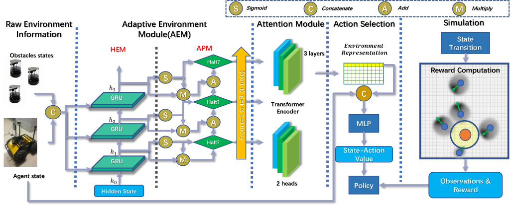
Figure 2: The system diagram of the proposed adaptive environment model RL (AEMCARL) based crowded-aware collision-free motion planning network. The first row with yellow color of the transformer encoder output means the global environment perception information of the robot, the other rows with white color correspond to the perception information of obstacles.

Fig. 2 illustrates the proposed RL-based navigation system with collision avoidance in crowded scenes for an unmanned robot. The experiment platform contains a Husky as the unmanned robot and a group of Turtlebots as mobile obstacles. All robots are equipped with UWB modules, along with stationary UWB anchors, for localization, as shown in Fig. 1. All the odometry readings, including poses and velocities, UWB readings, and action commands are exchanged through the ROS communication network. The Gym-based simulator [5] is used to train the hierarchical environment model (HEM), adaptive perception mechanism (APM), policy function, and evaluation network.

III-B Problem Statement

The state of the agent at time $t$ is denoted as $ego_{t}$ defined by Eq. 1, which includes velocity, $(\textit{$v_{x}^{a}$},~{}\textit{$v_{y}^{a}$})$, position, $(\textit{$x^{a}$},~{}\textit{$y^{a}$})$, goal position, $(\textit{$g_{x}^{a}$},~{}\textit{$g_{y}^{a}$})$, and preferred velocity, $v^{pref}_{r}$. The states of mobile obstacles at time $t$ is denoted as $\textit{{$o_{t}$}}\in\mathbb{R}^{N*D_{obs}}$ ($N$ is the number of obstacles, $D_{obs}$ is feature size of obstacle), which contains states of all obstacles include the velocity, $(\textit{$v_{x}^{o}$},~{}\textit{$v_{y}^{o}$})$, position, $(\textit{$x^{o}$},~{}\textit{$y^{o}$})$, and preferred velocity value, $v^{pref}_{o}$ defined by Eq. 1. The input of the RL network is the joint state of the agent and all obstacles, $\mathbf{s_{t}}=\textit{($ego_{t}$,$~{}o_{t}$)}\in\mathbb{R}^{(N+1)\times\left(D_{obs}+D_{agent}\right)}$. $\mathbf{s_{t}}$ contains the status of $N$ obstacles and an agent. The output of the RL network is an action noted as $\mathbf{a}$ composed by $v_{x}$ and  $v_{y}$.

$$ego_{t} =\left[v_{x}^{a},v_{y}^{a},x^{a},y^{a},g_{x}^{a},g_{y}^{a},v^{pref}_{a}\right],$$ (1)

$$o_{t} =\left[v_{x}^{o},v_{y}^{o},x^{o},y^{o},v^{pref}_{o}\right].$$

The objective of the RL learning is to find the optimal motion planning policy, $Q^{*}_{\pi}\left(\textit{$\textbf{$s_{t}$}$},\textit{{$a_{t}$}}\right):=max~{}Q_{\pi}\left(\textit{$\textbf{$s_{t}$}$},\textit{{$a_{t}$}}\right)$, as shown in Eq. 2 [5], which can enable the agent to reach the destination as soon as possible with low collision probability in crowded scenes.

$$Q^{*}_{\pi}\left(\textit{$\textbf{$s_{t}$}$},\textit{{$a_{t}$}}\right)= \underset{\mathbf{a}_{t}}{\operatorname{argmax}}R\left(\mathbf{s}_{t},\mathbf{a}_{t}\right)+$$ (2)

$$\gamma^{\Delta t\cdot v^{pref}}\int_{\mathbf{s}_{t+\Delta t}^{jn}}P\left(\mathbf{s}_{t},\mathbf{a}_{t},\mathbf{s}_{t+\Delta t}\right)V^{*}\left(\mathbf{s}_{t+\Delta t}\right)d\mathbf{s}_{t+\Delta t},$$

where $a_{t}$ is the action taken by the robot at the time $t$, $\gamma$ is the discount factor, $\gamma\in[0,1]$, and $V^{*}$ is the optimal state-action value obtained by the trained value network, $P\left(\mathbf{s}_{t},\mathbf{a}_{t},\mathbf{s}_{t+\Delta t}\right)$ is the probability of transiting to $\mathbf{s}_{t+\Delta t}$ from $\mathbf{s}_{t}$ and $\mathbf{a}_{t}$.

Specifically, this work focuses on solving the following problems:

1. How to develop a model to represent the dynamic interactions among multiple agents with high accuracy and efficiency;

2. How to reduce the computational complexity of the system through the adaptive perception and the attention modules;

3. How to achieve the collision-free robust motion planning policy using a proper reward function.

IV Proposed Methods

IV-A Hierarchical Environment Model

The action instantly taken by the agent is affected by both direct robot-to-obstacle interaction and potential obstacle-to-obstacle interaction. The goal of each obstacle in the real world is unpredictable and random. Inspired by the method [19], the proposed HEM consists of a number of GRUs to represent the dynamic environment of multiple mobile obstacles, as shown in Fig. 2. Each GRU [15] is given by

$$z_{t} =\sigma\left({\rm MLP}([h_{t-1},s_{t}],W_{z})\right),$$ (3)

$$r_{t} =\sigma\left({\rm MLP}([h_{t-1},s_{t}],W_{r})\right),$$

$$q_{t} =\tanh\left({\rm MLP}([r_{t}\odot h_{t-1},s_{t}],W_{q})\right),$$

$$h_{t} =\left(1-z_{t}\right)\odot h_{t-1}+z_{t}\odot q_{t},$$

where $s_{t}$ is the input state defined in Eq. 1, each MLP consists of two linear perception layers, and all these MLPs have the same structure. The output of each GRU is given by

$$h_{t}^{n}=\left\{\begin{array}[]{ll}{\rm GRU}(h_{0},s_{t}^{1}),&\textnormal{if }n=1\\ {\rm GRU}(h_{t}^{n-1},s_{t}^{n}),&\textnormal{otherwise}\end{array}\right.,$$ (4)

where $h_{0}$ is initialized by a zero vector, $n$ is the number of computation iterations of the HEM, and $h_{t}$ is the $t^{th}$ environment input of the HEM module. The HEM has three layers, and each includes a GRU. The execution order of these GRUs is serial, and each GRU takes the output of the previous GRU and raw environment state as input. The output of GRU will be used to determine whether the output is enough to represent the raw environment state or not, if enough, the serial execution will be terminated, otherwise, continue the serial execution. The details of how to decide if enough are introduced in Sec. IV-B.

Since the linear transformation operation, as shown in Eq. 5, is used as the MLP operation of GRU, the feature size of input shape, denoted by $\left(D_{obs}+D_{agent}\right)$, must be equal to the number of rows of the learnable weights, denoted by $\bf{W}$, which can make each GRU module to take the different number of obstacles.

$$y=xW+b,$$ (5)

where $x\in\mathbb{R}^{(N+1)\times(D_{obs}+D_{agent})}$ is the input, and $W\in\mathbb{R}^{(D_{obs}+D_{agent})\times D_{out}}$ is the the learnable weights, $b$ is the bias, and $y\in\mathbb{R}^{(N+1)\times D_{out}}$ is the output. The number of obstacles, $N$, does not affect the parameter of learnable weights.

IV-B Adaptive Perception Mechanism

Algorithm 1 AEM Module

0:    Input state = $s_{t}$, terminal state Nt = {$h_{t}^{n}\geq 1-\epsilon$}, and initialize the hidden state $h_{1}$

0:    

1:  for n = 1, N do

2:     Obtain the interaction features $h_{t}^{n}$ with the GRU

3:     Compute the believe probability $p_{t}^{n}$ of $h_{t}^{n}$ according to Eq. 6

4:     Update the sum of $p_{t}^{n}$ and $p_{t}^{n}h_{t}^{n}$, respectively

5:     if terminal state N(t) or $t\geq t_{max}$ then

6:        Break

7:     end if

8:  end for

8:    

9:  Return the output feature $y_{t}^{n}$ according to Eq. 7

The sigmoidal halting unit, $\sigma(\cdot)$, is added to the end of each GRU, as shown in Fig. 2. It can be used to determine whether the output of the AEM is sufficient to represent the dynamic environment or not through

$$p_{t}^{n}=\sigma\left(W^{h}h^{n}_{t}+b^{h}\right),$$ (6)

where $W^{h}$ represents the weight parameters, $b^{h}$ is the bias parameter and the parameters of this sigmoidal halting unit are trained within the whole framework. The output of the halting unit, given by Eq. 6, can also be used as the confidence of environment perception. The adaptive mechanism determines the number of GRUs in use according to the perception confidence and the halt parameter, that is,

$$y_{t}^{n} =\frac{1}{N(t)}\sum_{n=1}^{N(t)}p_{t}^{n}h_{t}^{n},$$ (7)

$$N(t) =\min\left\{n:\sum_{n=1}^{n}p_{t}^{n}\geq 1-\epsilon\right\},~{}\textit{s.t.}~{}n\geq 1,$$

where $N(t)$ is the adaptive number of GRUs, and $\epsilon$ is the halt threshold, $n$ is the maximum number of GRUs, and the perception confidence is $p_{t}^{n}$. The output of the AEM is $y_{t}^{n}\in\mathbb{R}^{(N+1)\times D_{AEM}}$ , given by Eq. 7 [19]. As we can see, the adaptive perception process is iterative, the final output is the weighted sum-up of all iterations’ result. The overall operation of the AEM module is shown in Algorithm 1.

IV-C Collision-free Policy Formulation

IV-C1 Reward Design

The reward is expected to be maximally returned by using the optimal policy. Compared to the existing reward functions  [5, 8, 9], our reward design is different in how to calculate the reward in complex situations and adaptively modulate the reward function according to the dynamic environment. Those reward design methods [5, 8, 9] just consider the closest obstacle and hence are not suitable to deal with variable numbers of obstacles.

$\begin{array}[]{cc}\begin{@subfigure}\includegraphics[height=130.08731pt]{same_speed_rewardv3}\end{@subfigure}&\begin{@subfigure}\includegraphics[height=130.08731pt]{different_speed_rewardv3}\end{@subfigure}\\ \end{array}$

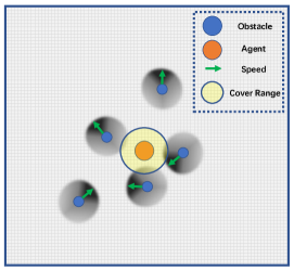
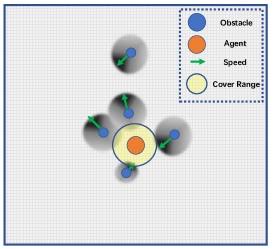
Figure 3: An illustration of the possible collision areas of 5 mobile obstacles moving randomly. The shaded areas representing the distribution of obstacles location is proportional to the current speed of each obstacle. The yellow area around the agent represents the agent coverage, therefore the overlap part in the shaded areas and agent coverage is the collision probability. (a) The obstacles are all in the same velocity with different orientations. The $p_{collision}$ is calculated between the agent and three obstacles. (b) The obstacles are in different velocities and orientations. The $p_{collision}$ is calculated between the agent and four obstacles.

By contrast, we use the predictive collision possibility ($p_{collision}$) between the agent and obstacles as the reward with unchanged agent and obstacles actions. As shown in Fig. 3, we estimate the distribution of obstacles’ position in the next time step by current position and velocity, and then the probability of obstacles in the agent’s coverage ($\phi_{agent}$) at the next time step is accumulated as the predictive collision possibility ($p_{collision}$). Due to the unpredictable dynamic environment, the reward function cannot be formulated by directly taking the predicted states (const velocity prediction) of the obstacles from the simulator with the long-range time step. And the time step in the reward function is bigger than that of the simulator settings. Therefore, our reward function is designed by

$$R_{t}\left(\mathbf{s}_{t},\mathbf{a}_{t}\right)=\left\{\begin{array}[]{cc}{1,}&{\text{~{}}\mathbf{Arrival}}\\ {-0.25,}&{\text{~{}}\mathbf{Collision}}\\ {-0.25p_{collision}\beta},&{\text{\bf{Otherwise}}}\\ \end{array}\right.,$$ (8)

where $p_{collision}=\sum_{(x,y)\in\phi_{agent}}g_{map}(x,y)$, $\phi_{agent}$ is the coverage of agent as shown in Fig. 3. $g_{map}(x,y)$ is the probability that the position $(x,y)$ is occupied by obstacles. $\beta$ is a hyper-parameter that is used to prevent the predictive collision possibility ($p_{collision}$) from being too small to cause the model performance degradation. $\mathbf{Arrival}$ means the distance between the agent and its target position is less than $0.1\text{\,}\mathrm{m}$. At time $t$, $g_{map}(x,y)$ can be computed by

$$g_{map}^{t}(x^{t},y^{t})=\sum_{i=1}^{N}g^{x}(x^{t}-x_{i}^{o})g^{y}(y^{t}-y_{i}^{o})g^{\theta}\left(\theta^{t}-\theta_{i}^{o}\right),$$ (9)

$$g^{x}=N(0,\delta_{x}),g^{y}=N(0,\delta_{y}),g^{\theta}=N(0,\delta_{\theta}),$$

$$\theta_{i}^{o}=\arctan(\frac{v_{i}^{y}}{v_{i}^{x}}),\theta^{t}=\arctan(\frac{y^{t}-y_{i}^{o}}{x^{t}-x_{i}^{o}})$$

where N is the number of obstacles, and $\delta_{x}$, $\delta_{y}$ and $\delta_{\theta}$ are hyper-parameters. $(x_{i}^{o},y_{i}^{o})$ is the position of the $i^{th}$ obstacle, and $\theta_{i}^{o}$ is the heading angle of the $i^{th}$ obstacle. $\theta^{t}$ is the angle between a line from $(x_{i}^{o},y_{i}^{o})$ to $(x^{t},y^{t})$ and the x-axis. As shown in Eq. 9, $g_{map}(x,y)$ is the cumulative probability of each obstacle at $(x,y)$.

For each obstacle, the probability that the obstacle is at $(x,y)$ is calculated by ${g^{x}(x^{t}-x^{o})g^{y}(y^{t}-y^{o})g^{\theta}}(\theta^{t}-\theta^{o})$ as shown in Eq. 9. To simplify the calculation, we just consider a circular area centered on the current position of the obstacle. The radii of the circular area and $\phi_{agent}$ are $v^{o}\Delta\mathbf{t_{obstacle}}$ and $v^{a}\Delta\mathbf{t_{agent}}$ respectively, where $\Delta\mathbf{t_{obstacle}}$ and $\Delta\mathbf{t_{agent}}$ are hyper-parameters which indicate the time prediction length. As shown in Fig. 3, circular areas have different radii because obstacles have different speeds. We also build a grid map that the value of each grid is $g_{map}(x,y)$, and this grid map changes over time.

IV-C2 Policy Formulation

Algorithm 2 AEMCARL

0:    Obtain the terminal state: {Reaching the goal, Collision}Generate training state-action samples $\mathcal{S}$ using the ORCA method, and the memory unit $\mathcal{\hat{M}}\leftarrow\mathcal{S}$ Initialize the value network, $\mathcal{V}\leftarrow\mathcal{S}$, the target value network $\mathcal{\hat{V}}\leftarrow\mathcal{V}$

0:    

1:  for epoch = 1, N  do

2:     Initialize random samples $s^{0}$ from $\mathcal{\hat{M}}$

3:     repeat

4:        Formulate the interaction feature $s_{IN}$ with the AEM

5:        Compute the environment feature with the TFM

6:        Update the value network $\mathcal{V}$ with the action module

7:        if terminal state $s_{t}$ then

8:           Update the memory unit $\mathcal{\hat{M}}$

9:        end if

10:     until terminal state $s_{t}$ or $t\geq t_{max}$

11:     Update the target network $\mathcal{\hat{V}}\leftarrow\mathcal{V}$

12:  end for

12:    

13:  Return $\mathcal{V}$

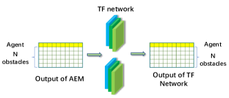
Figure 4: An illustration of the workflow of the TF network. The input of TF network $y_{t}^{n}\in\mathbb{R}^{(N+1)*D_{AEM}}$, and TF nwtwork does not change the order of input. features

The attention mechanism can help improve the collision-free navigation performance of the model. The Transformer (TF) Network [16] can adaptively extract the most important information of features according to the self-attention mechanism, and adopt the multi-head mechanism to estimate more reliable features. The self-attention of the TF module is given by [16]

$$\left\{\begin{array}[]{l}\mathbf{Q}={\rm MLP}\left(W^{q}y_{t}^{n}+b^{q}\right),\\ \mathbf{K}={\rm MLP}\left(W^{k}y_{t}^{n}+b^{k}\right),\\ \mathbf{V}={\rm MLP}\left(W^{v}y_{t}^{n}+b^{v}\right),\\ \mathbf{Att}\left(Q,K,V\right)={\rm softmax}\left(\frac{QK^{T}}{\sqrt{d_{k}}}\right)V,\\ \end{array}\right.$$ (10)

where the output order of the AEM modules is from top to bottom. $y_{t}^{n}\in\mathbb{R}^{(N+1)*D_{AEM}}$ is the output of AEM. $d_{k}$ is the dimension of the feature, $Q,K,V$ are three feature embedding layers [16].

As shown in Fig. 4, TF network does not change the order of input features and weights each feature with other features by an attention mechanism. Among the $N+1$ features output by TF network, the first feature is the joint state representation of the agent and other obstacles. We only extract the first row of the output of the attention module, $\mathbf{Att}\left(Q,K,V\right)$, as shown the first yellow row at the right of Fig. 2 and Fig. 4. This is the reason we train in an environment with 5 obstacles but can perform well in an environment with 20 obstacles.

Therefore, the features of environment, $y_{t}^{n}$, are fed into the TF module (TFM) to help achieve collision-free decisions for possible partial observations. The TF output, denoted by $f_{TF}$, is used to represent the feature of multi-agent interactions. The input robot state, $s^{t}_{agent}$, is concatenated with the embedding feature, $f_{TF}$, to construct the final environment feature, given by Eq. 11.

$$v^{t}_{action}={\rm MLP}\left(\left[f_{TF}\oplus s^{t}_{agent}\right]\right),$$ (11)

where $\bigoplus$ means the concatenation operation. The overall procedure of our proposed reinforcement learning of collision-free motion planning policy is shown in Algorithm 2.

IV-D Model Training

We use the same cost function as DQN to train the framework including AEM (HEM, APM) and TFM. As with other deep learning algorithms, the model is trained by combining the cost function with the gradient backpropagation for parameter updating.

IV-E Computation Setup

The key parameters of the RL network include: discount factor $\gamma$ = 0.9, batch size $batch$ = 100, learning rate $L$ = 0.001, halt parameter $\epsilon$=0.05, collision scale ratio $\beta$ = 2.0, and optimism method being Adam [23]. In our setup, we let $\delta_{x}$ be the same as $\delta_{y}$, denoted as $\delta_{xy}$. The variances of the obstacle position, denoted by $\delta_{xy}$, and heading angle, denoted by $\delta_{\theta}$, are set as 2, respectively. The hidden units of AEM module, TF module, and action module are [(100, 50)], [(150, 150, 150), $nhead$:2], and [(150, 100, 100, 1)], respectively. The action space consists of 80 discrete actions: 5 speeds exponentially distributed over $(0,v^{pref}]$ and 16 orientations evenly distributed over $[0,2\pi)$.

V Experiments

The simulation experiments were performed on a PC with an Intel core i7-7700K CPU, an Nvidia GTX1070 GPU, and 32G RAM. In the physical experiments, we used a portable computation platform with an Intel core i5-5500T CPU, and 16G RAM. There were two testing cases for the unmanned robot navigation with multiple mobile obstacles: invisible and visible. The former means that all obstacles cannot detect the unmanned robot; whereas the latter means that they can. Since the obstacle robots are operated by the ORCA [7] method that enables robots to actively avoid obstacles. The invisible case is to ensure that the obstacle robots cannot actively avoid the unmanned robot, which is used to demonstrate the collision-free performance of the proposed AEMCARL.

V-A Quantitative Evaluation

TABLE II: A COMPARISON OF NAVIGATION PERFORMANCE BETWEEN THE STATE-OF-THE-ART METHODS AND OUR METHOD

Methods	Success Rate	Collision Rate	Time (s)	Timeout Rate
ORCA [7]	0.43	0.57	10.93	0.00
LM-SARL-Linear [5]	0.90	0.09	11.15	0.01
RGL-Linear [4]	0.91	0.01	10.37	0.08
MP-RGL-Onestep [4]	0.92	0.02	10.44	0.06
MP-RGL-MultiStep [4]	0.97	0.01	$10.95$	0.02
AEMCARL (Ours)	1.00	0.00	11.09	0.00

All experiments are based on one invisible unmanned robot and five mobile obstacles. The AEMCARL in table adopts the designed adaptive reward function.

The invisible case is more challenging for collision-free navigation than that of the visible case. TABLE II shows a comparison between the state-of-the-art methods and our method. To validate the performance of the proposed method, the baseline methods are selected by following the rule that all state-of-the-art (SOTA) methods are trained by the same simulator and trained from scratch by ourselves. The comparison is based on 5 obstacles for invisible cases with 500 random experiments. It can be seen that our method is the most robust one to reach the goal with the smallest collision probability. The last column of TABLE II shows that our method can accomplish the task each time within the predefined time which is set as 20 seconds. As shown in 6, the RGL [4] methods are with the poorest generalization for the scenes with more obstacles (e.g. $n\geq 5$ ). As shown in TABLE II, the proposed method outperforms the other baseline methods with narrow improvements and total success rate. However, the proposed method can also keep the robustness to the more complex scenes that include more obstacles of different sizes shapes, and velocities, as shown in Fig. 6.

The Time metric in TABLE II means the average time with 500 random experiments. Except for the time limits of RGL variants methods being set 30 seconds, the other methods are 20 seconds. The Time-out metric means the ratio of the experiments without reaching the destination in the allowed maximum time of the methods, accordingly.

$\begin{array}[]{cc}\begin{@subfigure}\includegraphics[height=108.405pt]{egru-rate_inv_4_8}\end{@subfigure}&\begin{@subfigure}\includegraphics[height=108.405pt]{egru-rate_v_4_8}\end{@subfigure}\\ \begin{@subfigure}\includegraphics[height=108.405pt]{sr-cases-iv-gru}\end{@subfigure}&\begin{@subfigure}\includegraphics[height=108.405pt]{sr-cases-v-gru}\end{@subfigure}\\ \end{array}$

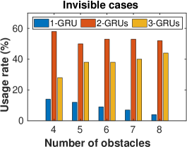
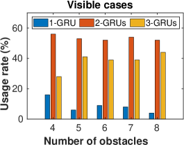
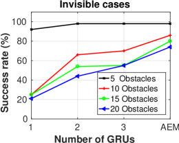
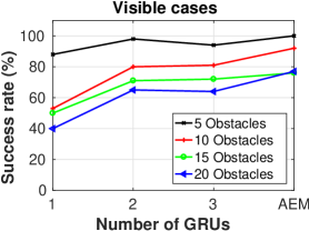
Figure 5: An illustration of AEM operations in AEMCARL. (a & b) An illustration of the usage rates of GRUs in AEMCARL for different numbers of obstacles in invisible (a) and visible (b) cases, respectively. (c & d) The success rates of the AEMCARL using different fixed numbers of GRUs and the adaptive mechanism (AEM), for different numbers of obstacles in invisible (c) and visible (d) cases, respectively.

V-B Ablation Study

V-B1 AEM Efficiency

$\begin{array}[]{ccc}\begin{@subfigure}\includegraphics[height=130.08731pt]{reward_paras}\end{@subfigure}&\begin{@subfigure}\includegraphics[height=130.08731pt]{sr}\end{@subfigure}&\begin{@subfigure}\includegraphics[height=130.08731pt]{freq}\end{@subfigure}\\ \end{array}$

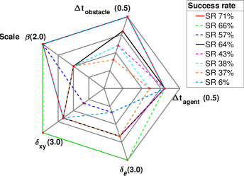
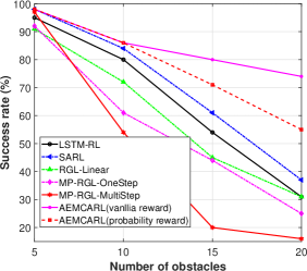
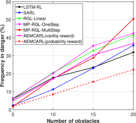
Figure 6: The evaluation of AEMCARL. (a) A comparison of the navigation success rates using different parameters in the case of 20 obstacles with 50 random experiments. The number in the bracket means the maximum value of the corresponding radius. (b) A comparison of the navigation success rates using LSTM-RL, SARL, RGL-Linear, MP-RGL-OneStep, MP-RGL-MultiStep, and AEMCARL for different numbers of obstacles. (c) A comparison of frequency in danger using LSTM-RL, SARL, RGL-Linear, MP-RGL-OneStep, MP-RGL-MultiStep, and AEMCARL for different numbers of obstacles.

Our approach was also tested with real-world experiments in different scenarios using 4 to 8 mobile obstacles, respectively. Turtlebots were used as mobile obstacles and a Husky was used as the unmanned robot that performed the RL-based collision-free navigation, as shown in Fig. 1. Fig. 5 and Fig. 5 show the usage rate of 3 GRUs for different scenarios in the real world, which can be seen in the appendix video material. It can be seen that the proposed adaptive perception module (APM) can automatically change the structure of the hierarchical environment module (HEM) in different scenarios to optimize the framework of the neural network.

Both SARL and AEMCARL use the attention mechanism to focus on the most threatening obstacles, which helps them to achieve fast training convergence and best navigation performance in the case of a different number of obstacles (TABLE II). The adaptive perception module can further help AEMCARL to improve the computation speed without losing the navigation performance. Fig. 5 and Fig. 5 show a comparison of navigation performance between using 3 different fixed numbers of GRUs and the adaptive perception mechanism (AEM) given a different number of obstacles for 100 random experiments of both visible and invisible cases. It can be seen that the AEM outperforms any fixed number of GRUs.

V-B2 Reward Design

The proposed adaptive reward function contains multiple parameters, as shown in Fig. 6. To study the role of each parameter in the reward function, we conducted a set of experiments to compare the performance of each parameter with 100 random experiments under the model trained by only 2000 episodes. The success rate was used as the performance indicator. Fig. 6 shows that the parameters, including $\Delta$$\mathbf{t_{agent}}$, $\Delta$$\mathbf{t_{obstacle}}$, and $\mathbf{Scale~{}\beta}$, basically are proportional to the success rate. Since the hyperparameters ($\mathbf{\delta_{xy}}$, $\mathbf{\delta_{\theta}}$) are used to tune the expectation of the squared deviation of the mean of the velocity and heading angle. So the relationships between $\mathbf{\delta_{xy}}$$\setminus$$\mathbf{\delta_{\theta}}$ and the success rate are not monotonous.

V-B3 Policy Efficiency

Both Fig. 6 and Fig. 6 show the comparison of system performance for different numbers of obstacles in the same size between three open-source baseline RL methods (LSTM-RL, SARL and RGL) and our method with 100 random experiments.  Fig. 6 shows the success rate of baseline methods dramatically degrades with the increase of the number of obstacles. The vanilla reward in Fig. 6 is the same as SARL. Compared to the vanilla reward, our adaptive reward based probability with the highest success rate in the cases of a different number of obstacles. In addition, the AEMCARL with the vanilla reward outperforms the state-of-the-art (SOTA) methods, SARL and RGL, which can demonstrate the efficiency of the framework of our model. SARL and RGL use two different methods to represent the obstacles states in the environment: the attentive pooling mechanism and the relational graph learning approach, respectively. Our proposed reward function and model framework can adapt to different environments, which can increase the robustness of the collision-free RL model.

V-B4 Policy Robustness

The proposed method, AEMCARL, was trained in the gym simulator with 5 obstacles, but our trained policy, AEMCARL, was tested in the environment cases with multiple obstacles $\left(\geq 5\right)$. As shown in TABLE II, Fig. 6 and Fig. 6, our proposed method outperforms the SOTA methods in 5, 10, 15, and 20 obstacles environments without tuning, which can demonstrate the robustness of the proposed method.

The frequency in danger means the ratio between the number of minimum agent-to-object separation distances lower than the threshold and the total number of actions. It can reflect the degree of aggressiveness policies when processing the danger cases. Thanks to AEM, adaptive reward function, and TF module, Fig. 6 and Fig. 6 show that our method outperforms the two baseline methods in terms of both success rate and frequency in danger.

VI CONCLUSION

This paper has presented an adaptive environment modeling-based reinforcement learning (AEMCARL) network which focuses on (1) dynamic environment representation, (2) adaptive perception mechanism, and (3) adaptive reward function for collision-free motion planning policy. The proposed hierarchical environment model (HEM) can robustly and efficiently model the dynamic environment. The adaptive perception mechanism (APM) can adaptively use computational resources within a certain degree of perception confidence. The reward function can adaptively modulate the reward according to the relation between the robot with the real-time environment. The simulation experiment results show that by training with 5 obstacles and testing with 20 ones, (1) our proposed algorithm can achieve at least 74% of success rate, which is 37% higher than the SOTA algorithms, and achieve the lowest frequency in danger; (2) compared with policies using a different fixed number of GRUs, our AEM can get the best performance in terms of success rate. Our future work will further investigate the computational efficiency as well as relationships between perception/planning complexities of the environment and RL models.

References

- [1] Y. F. Chen, M. Everett, M. Liu, and J. P. How, “Socially aware motion planning with deep reinforcement learning,” in 2017 IEEE/RSJ International Conference on Intelligent Robots and Systems (IROS). IEEE, 2017, pp. 1343–1350.
- [2] X. Ma, J. Li, M. J. Kochenderfer, D. Isele, and K. Fujimura, “Reinforcement learning for autonomous driving with latent state inference and spatial-temporal relationships,” in 2021 IEEE International Conference on Robotics and Automation (ICRA). IEEE, 2021, pp. 6064–6071.
- [3] R. Han, S. Chen, S. Wang, Z. Zhang, R. Gao, Q. Hao, and J. Pan, “Reinforcement learned distributed multi-robot navigation with reciprocal velocity obstacle shaped rewards,” IEEE Robotics and Automation Letters, vol. 7, no. 3, pp. 5896–5903, 2022.
- [4] C. Chen, S. Hu, P. Nikdel, G. Mori, and M. Savva, “Relational graph learning for crowd navigation,” in 2020 IEEE/RSJ International Conference on Intelligent Robots and Systems (IROS). IEEE, 2020, pp. 10 007–10 013.
- [5] C. Chen, Y. Liu, S. Kreiss, and A. Alahi, “Crowd-robot interaction: Crowd-aware robot navigation with attention-based deep reinforcement learning,” in 2019 International Conference on Robotics and Automation (ICRA). IEEE, 2019, pp. 6015–6022.
- [6] J. Van den Berg, M. Lin, and D. Manocha, “Reciprocal velocity obstacles for real-time multi-agent navigation,” in 2008 IEEE International Conference on Robotics and Automation. IEEE, 2008, pp. 1928–1935.
- [7] J. Alonso-Mora, A. Breitenmoser, M. Rufli, P. Beardsley, and R. Siegwart, “Optimal reciprocal collision avoidance for multiple non-holonomic robots,” in Distributed autonomous robotic systems. Springer, 2013, pp. 203–216.
- [8] M. Everett, Y. F. Chen, and J. P. How, “Motion planning among dynamic, decision-making agents with deep reinforcement learning,” in 2018 IEEE/RSJ International Conference on Intelligent Robots and Systems (IROS). IEEE, 2018, pp. 3052–3059.
- [9] Y. F. Chen, M. Liu, M. Everett, and J. P. How, “Decentralized non-communicating multiagent collision avoidance with deep reinforcement learning,” in 2017 IEEE international conference on robotics and automation (ICRA). IEEE, 2017, pp. 285–292.
- [10] Y. Chen, C. Liu, B. E. Shi, and M. Liu, “Robot navigation in crowds by graph convolutional networks with attention learned from human gaze,” IEEE Robotics and Automation Letters, vol. 5, no. 2, pp. 2754–2761, 2020.
- [11] L. Liu, D. Dugas, G. Cesari, R. Siegwart, and R. Dubé, “Robot navigation in crowded environments using deep reinforcement learning,” in 2020 IEEE/RSJ International Conference on Intelligent Robots and Systems (IROS). IEEE, 2020, pp. 5671–5677.
- [12] P. Battaglia, R. Pascanu, M. Lai, D. J. Rezende, et al., “Interaction networks for learning about objects, relations and physics,” in Advances in neural information processing systems, 2016, pp. 4502–4510.
- [13] S. Hochreiter and J. Schmidhuber, “Long short-term memory,” Neural computation, vol. 9, no. 8, pp. 1735–1780, 1997.
- [14] J. Li, F. Yang, H. Ma, S. Malla, M. Tomizuka, and C. Choi, “Rain: Reinforced hybrid attention inference network for motion forecasting,” in Proceedings of the IEEE/CVF International Conference on Computer Vision, 2021, pp. 16 096–16 106.
- [15] K. Cho, B. Van Merriënboer, C. Gulcehre, D. Bahdanau, F. Bougares, H. Schwenk, and Y. Bengio, “Learning phrase representations using rnn encoder-decoder for statistical machine translation,” arXiv preprint arXiv:1406.1078, 2014.
- [16] A. Vaswani, N. Shazeer, N. Parmar, J. Uszkoreit, L. Jones, A. N. Gomez, Ł. Kaiser, and I. Polosukhin, “Attention is all you need,” in Advances in neural information processing systems, 2017, pp. 5998–6008.
- [17] A. Vemula, K. Muelling, and J. Oh, “Social attention: Modeling attention in human crowds,” in 2018 IEEE international Conference on Robotics and Automation (ICRA). IEEE, 2018, pp. 4601–4607.
- [18] A. J. Sathyamoorthy, J. Liang, U. Patel, T. Guan, R. Chandra, and D. Manocha, “Densecavoid: Real-time navigation in dense crowds using anticipatory behaviors,” in 2020 IEEE International Conference on Robotics and Automation (ICRA). IEEE, 2020, pp. 11 345–11 352.
- [19] A. Graves, “Adaptive computation time for recurrent neural networks,” arXiv preprint arXiv:1603.08983, 2016.
- [20] J. Schulman, F. Wolski, P. Dhariwal, A. Radford, and O. Klimov, “Proximal policy optimization algorithms,” arXiv preprint arXiv:1707.06347, 2017.
- [21] V. Mnih, A. P. Badia, M. Mirza, A. Graves, T. Lillicrap, T. Harley, D. Silver, and K. Kavukcuoglu, “Asynchronous methods for deep reinforcement learning,” in International conference on machine learning, 2016, pp. 1928–1937.
- [22] A. J. Sathyamoorthy, U. Patel, T. Guan, and D. Manocha, “Frozone: Freezing-free, pedestrian-friendly navigation in human crowds,” IEEE Robotics and Automation Letters, vol. 5, no. 3, pp. 4352–4359, 2020.
- [23] D. P. Kingma and J. Ba, “Adam: A method for stochastic optimization,” arXiv preprint arXiv:1412.6980, 2014.