Some Aspects of Rotation and Magnetic Field Morphology in the Infrared Dark Cloud G34.43+00.24

Abstract

The infrared dark clouds (IRDCs) are molecular clouds with relatively greater values in their magnetic field strengths. For example, the IRDC G34.43+00.24 (G34) has magnetic field strength of the order of a few hundred micro-Gauss. In this study, we investigate if the dynamic motions of charged particles in an IRDC such as G34 can produce this magnetic field strength inside it. The observations show that the line-of-sight velocity of G34 has global gradient. We assume that the measured global velocity gradient can correspond to the cloud rotation. We attribute a large-scale current density to this rotating cloud by considering a constant value for the incompleteness of charge neutrality and the velocity differences between the positive and negative particles with very low ionization fractions. We use the numerical package FISHPACK to obtain the magnetic field strength and its morphology on the plane-of-sky within G34. The results show that the magnetic field strengths are of the order of several hundred micro-Gauss, and its morphology in the plane-of-sky is somewhat consistent with the observational results. We also obtain the relationship between magnetic field strength and density in G34. The results show that with increasing density, the magnetic field strength increases approximately as a power-law function. The amount of power is approximately equal to $0.45$, which is suitable for molecular clouds with strong magnetic fields. Therefore, we can conclude that the dynamical motion of IRDCs, and especially their rotations, can amplify the magnetic field strengths within them.

1 Introduction

The infrared dark clouds (IRDCs) were discovered three decades ago, as silhouettes against a bright infrared background, by the Infrared Space Observatory (Perault et al. 1996) and the Midcourse Space Experiment (Egan et al. 1998). Carey et al. (1998) were the first group to study the physical properties of IRDCs after their discovery. They investigated $10$ observed clouds, all $1$ to $8\,\mathrm{kpc}$ away from us, with diameters ranging from $0.4$ to $15\,\mathrm{pc}$. Their analysis on the extinction of the observed lines indicated that the IRDCs are cold and dense regions, with temperatures less than $20\,\mathrm{K}$ and density larger than $10^{5}\,\mathrm{cm}^{-3}$. Rathborne et al. (2006) scrutinized the millimeter continuum maps of $38$ IRDCs in our galaxy. These clouds range in morphology from filamentary to compact and have masses of $120$ to $16000\,\mathrm{M}_{\odot}$. Within these IRDCs, they also found $140$ cores, with masses in the range of $10-2100\,\mathrm{M}_{\odot}$, which their mass spectrum slope was similar to that of the stellar IMF. Therefore, they concluded that IRDCs could be suitable precursors to form stellar clusters and massive stars. The observations show that the IRDCs are magnetized molecular clouds. By developing the observational techniques in the last decade, more information about the magnetic field morphology in the IRDCs has been obtained (e.g., Santos et al. 2016, Hoq et al. 2017, Beuther et al. 2018, Juvela et al. 2018, Liu, Zhang, & Qiu et al. 2020, Añez-López et al. 2020).

One interesting IRDC is G34.43+00.24 (hereafter G34), which for the first time had been probed by Rathborne et al. (2005). This cloud, which is $3.6\,\mathrm{kpc}$ away from us and is located on the Galactic plane, has a filamentary clumpy structure (e.g., Liu, Sanhueza & Liu et al. 2020, Isequilla et al. 2021). Four major clumps of the G34 are known as MM1-MM4, which are nurseries for star formation with masses between $330$ and $1500\,\mathrm{M}_{\odot}$ and number densities between $1.8\times 10^{4}$ and $3.9\times 10^{5}\,\mathrm{cm}^{-3}$ (Sanhueza et al. 2010). By developing technology and receiving observational information on the smaller scales of the IRDCs, Jones et al. (2016) used FORCAST on SOFIA and submillimeter polarimetry to probe inside the MM1 clump of the G34. Their observations showed that G34 is embedded in an external magnetic field parallel to the Galactic plane and that the magnetic field inside MM1 is perpendicular to the long axis of G34.

Observational information, such as velocity, density, magnetic field, etc., corresponds to the projected information of the 3D medium. The projection is made along the line-of-sight generating a 2D plane-of-sky field. Tang et al. (2019) used thermal dust polarization at $350\mu\mathrm{m}$ with an angular resolution of $10^{\prime\prime}$ ($0.18\,\mathrm{pc}$) to observe the plane-of-sky magnetic field morphology across G34. Their investigations showed that the $B$-fields across the clumps MM1 and MM2 are mostly perpendicular to the filament’s axis, with a prevailing orientation around $70^{\circ}$. The MM3, oriented with its longer axis about $40^{\circ}$ off the north-south axis, reveals a $B$-field that is changing its orientation to close to parallel to the clump’s dust ridge. Soam et al. (2019) also used $850\,\mu\mathrm{m}$ polarized dust emission at the James Clerk Maxwell telescope to present the $B$-fields 2D mapped in G34. They obtained the plane-of-sky magnetic field strengths of $470\pm 190\,\mu\mathrm{G}$, $100\pm 40\,\mu\mathrm{G}$, and $60\pm 34\,\mu\mathrm{G}$ in the central, northern, and southern regions of G34, respectively.

All the observational data show that the magnetic field strengths in the IRDCs are of the order of several hundred $\mu\mathrm{G}$. On the other hand, we know that all the interstellar clouds and also IRDCs are immersed in the Galactic magnetic fields. The strengths of the magnetic fields in the Galactic plane are of the order of several $\mu\mathrm{G}$ (Jansson & Farrar 2012). Now the question is, what is the reason for the increase in magnetic field strength from the order of a few $\mu\mathrm{G}$ outside an IRDC to a few hundred $\mu\mathrm{G}$ inside? One way to answer this question is to use the topic of flux freezing in the ideal MHD. In a way that if an IRDC is formed from a diffuse ISM due to compression, with assuming the flux freezing, an increase in density from $n_{i}$ to $n_{f}$ can increase the magnetic field by $B_{f}\sim B_{i}(n_{f}/n_{i})^{2/3}$ (e.g., Mestel 1966). But the ionization fraction in the molecular clouds (such as IRDCs) is low, and the non-ideal MHD effects (such as ambipolar diffusion) are impressive (e.g., Hennebelle & Inutsuka 2019). On the other hand, we know that an IRDC has dynamic motions and is ionized by various mechanisms so that it contains moving ions, electrons, and charged grains. So we are looking for another possible answer based on the dynamic motions of the IRDCs and the electric currents created by the charged particles. Despite the low ionization fraction in an IRDC, can the dynamic motions of these charged particles amplify the magnetic field strengths within it? In this research we try to answer this question.

In this paper, we focus our attention on the dynamic motions and magnetic fields of the G34, of which we currently have suitable observational information. We want to know if the dynamic motions of this typical IRDC can increase the large-scale magnetic field strengths within it? For this purpose, in section 2, we extract the dynamic motions of the G34 from observational data and investigate its rotation. We attribute a large-scale current density to this rotating cloud by considering the velocity differences between the positive and negative particles with very low ionization fractions. The magnetic field resulting from this current density is obtained in § 3 and is compared with the observational results. Finally, § 4 is dedicated to summary and conclusion.

2 Rotation and Current Density

The molecular clouds are affected by various factors for ionization. One of these ionizing factors is the cosmic rays, that in a steady ionization equilibrium, lead to $\bar{n}_{i}\sim 7.5\times 10^{-3}(n_{n}/10^{3}\mathrm{cm}^{-3})^{1/2}$, where $\bar{n}_{i}$ and $n_{n}$ are the mean number densities of ions and neutral particles in the unit of $\mathrm{cm}^{-3}$, respectively (e.g., Shu 1992, p. 362). Priestley, Wurster & Viti (2019) have recently investigated differences in the molecular abundances and found that the mean number density of ions follows an approximate power-law relation with the number density of neutral particles as

$$\bar{n}_{i}\sim 10^{-4}\left(\frac{n_{n}}{10^{3}\mathrm{cm}^{-3}}\right)^{0.4}\,\mathrm{cm}^{-3}.$$ (1)

One of the remarkable interstellar molecular ion is $\mathrm{N}_{2}\mathrm{H}^{+}$, which is widely used as suitable tracer molecules in the study of molecular clouds (Thaddeus & Turner 1975). The abundance and distribution of $\mathrm{N}_{2}\mathrm{H}^{+}$ is well explained by the ion-molecule chemistry (Womack, Ziurys & Wyckoff 1992). The integrated emission of the $\mathrm{N}_{2}\mathrm{H}^{+}$ line can provide suitable situations for determining the $\mathrm{H}_{2}$ density in the molecular clouds and vice versa. Here, we use the integrated emission of the $\mathrm{N}_{2}\mathrm{H}^{+}$ line detected by Tang et al. (2019, Figure 3) for the IRDC G34. The $\mathrm{N}_{2}\mathrm{H}^{+}$ line intensity is actually proportional to the column density along the line-of-sight. We assume that G34 has a uniform slab geometry in the line-of-sight direction so that the column density implicitly represents the volume density. Womack, Ziurys & Wyckoff (1992) concluded that the fractional abundances of $\mathrm{N}_{2}\mathrm{H}^{+}$, relative to H2, is $\sim 4\times 10^{-10}$ toward both the warm and cold clouds. Thus, we assume that the fractional abundance of this ion, relative to the hydrogen molecules, is constant across the G34. We divide Figure 3 of Tang et al. (2019) into $17\times 58$ square pixels with side $\sim 0.16\,\mathrm{pc}$. Sanhueza et al. (2010) worked on the clumps in the G34 region and concluded that their number densities are between $1.8\times 10^{4}\,\mathrm{cm}^{-3}$ to $3.9\times 10^{5}\,\mathrm{cm}^{-3}$. On the other hand, in general, the number density around the molecular clouds drops to $10^{2}\,\mathrm{cm}^{-3}$ (e.g., Ballesteros-Paredes et al. 2020). Therefore, here, we assume that the $\mathrm{H}_{2}$ density in the centers of the clumps MM1, MM2, and MM3 of G34, is in the order of $10^{5}\,\mathrm{cm}^{-3}$, and in the outer and more distant periphery of G34, the number density of neutral particles drops to $10^{2}\,\mathrm{cm}^{-3}$. In this way, we consider the outermost contour in the Figure 3 of Tang et al. (2019) as the periphery of G34 and assign a density of $10^{2}\,\mathrm{cm}^{-3}$ to this contour. We also assign the innermost contour to the density of $10^{5}\,\mathrm{cm}^{-3}$. Assuming a simple linear relationship between the integrated emission of the $\mathrm{N}_{2}\mathrm{H}^{+}$ line and the column density, we can determine the number density of neutral particles assigned to the other contours. Thus, according to the number density of neutral particles obtained from the integrated emission of the $\mathrm{N}_{2}\mathrm{H}^{+}$ line, and the correlation relation between ion and neutral particle densities as outlined by the equation (1), we can determine the mean number density of ions inside G34. The result is shown in Fig. 1 as a contour color-fill map.

The right ascension and declination of the center of G34 is approximately equal to $RA=18\,\mathrm{h}\,53\,\mathrm{m}\,20\,\mathrm{s}=283.3^{\circ}$ and $DEC=+1^{\circ}\,26^{\prime}=1.43^{\circ}$ , which in the galactic coordinates is equal to $l=+34.42^{\circ}$ and $b=+0.23^{\circ}$. Stars and interstellar matters closer to the Galactic center complete their orbits in less time than those of the others further out. According to the Galactic longitude of G34, we can deduce that it moves away from us so that the measured line-of-sight centroid velocities present the red-shift motion of the cloud gas (e.g., Sparke & Gallagher 2007). Tang et al. (2019) extracted the kinematic information of the G34 using the $\mathrm{N}_{2}\mathrm{H}^{+}\;(J=1-0)$ line. Their centroid velocity map is very robust, with a typical velocity uncertainty of $\simeq 0.1\,\mathrm{km\,s}^{-1}$. They reported the maps of the centroid velocity and the dispersion of the $\mathrm{N}_{2}\mathrm{H}^{+}$ line in Figure 3. The results show that the G34 presents a very organized velocity field throughout the filament. The velocity gradient is along with the East-West direction, consistent with measurements in $\mathrm{N}\mathrm{H}_{3}$ at a higher angular resolution of $3^{\prime\prime}$ by Dirienzo et al. (2015).

If we assume that the filamentary structure of G34 is created by the shock compression of a turbulent inhomogeneous molecular cloud (e.g., Inoue et al. 2018), the velocity gradient perpendicular to the filament axis can be considered as tracing the matter flow onto a sheet-like structure (e.g., Arzoumanian et al. 2018). Here we consider another possible choice in which the velocity gradient is related to the rotation. If we assume that the materials of G34 were rotating as a bulk body with its rotation axis perpendicular to the line-of-sight, the measured velocity gradient would correspond to $\Omega$, the cloud’s angular velocity. A velocity gradient of magnitude $\sim 1.7\,\mathrm{km}\,\mathrm{s}^{-1}\,\mathrm{pc}^{-1}$, from left to right in Figure 3 of Tang et al. (2019), can be seen. This value implies that G34 rotates slowly with a representative period of $2\pi/\Omega\sim 3.5\times 10^{6}\,\mathrm{yr}$. We divide the right ascension direction in Figure 3 of Tang et al. (2019) into 17 pixels and the declination direction into 58 pixels. We extract the line-of-sight centroid velocity for each pixel and subtract it from their median value. These relative velocities for each pixel (relative to the median value) are shown in Fig. 2 as color-pixel-map. As shown in the figure, a hypothetical line can be passed through some pixels that have an approximately zero relative velocity (the median value). This assumptive line can represent the axis of rotation, which is shown in Fig. 2, and is approximately parallel to the plane of Galaxy (with an angle near to $9.2^{\circ}$). Thus, it can be visualized that the G34 rolls around the plane of the Galaxy like a rolling cylinder with a slow angular velocity $\Omega\sim 5.7\times 10^{-14}\,\mathrm{s}^{-1}$, and this rolling represents part of the Galaxy’s rotation around its center.

The moving charged particles with density $n$, electric charge $q$, and velocity $\mathbf{v}$ can produce a current density as $\mathbf{J}=nq\mathbf{v}$. The true current density in IRDCs is carried by a minor fraction of charged species: free electrons, ions, and grains. Since the number density of grains is so low that they contribute negligibly to the current, we have

$$\mathbf{J}=\sum_{i}n_{i}q_{i}\mathbf{v}_{i}-n_{e}e\mathbf{v}_{e},$$ (2)

where $n_{i}$ is the number density of each species of ions with charge $q_{i}$ and velocity $\mathbf{v}_{i}$. The number density of free electrons, with charge $e$ and velocity $\mathbf{v}_{e}$, is denoted as $n_{e}$. If we demand an ideal complete charge neutrality through the G34, we have $n_{e}\approx\sum_{i}n_{i}(q_{i}/e)$. But, in the real world, the charge neutrality is not complete. Also, there is not enough information about the velocities of electrons and various ions in G34. Here, we assume that the ions are well coupled with the neutral matter of the cloud and move with velocity $\mathbf{v}$. In this model, the free electrons can move forward or backward more quickly. In this way, according to the lack of information, we approximately apply the relation $J_{\perp}\approx\zeta e\bar{n}_{i}v_{\perp}$ for the current density component along the line-of-sight, where $\zeta$ has a positive and/or negative value depending on the non-completeness of charge neutrality and the relative speed of ions and electrons at each location of the cloud, and $v_{\perp}$ is the velocity along the line-of-sight (such as one which is deduced from $\mathrm{N}_{2}\mathrm{H}^{+}$ molecules in G34, and is depicted in Fig. 2).

To our knowledge, there is not as much research on the electric currents in the interstellar medium, but we can refer to the article Carlqvist & Gahm (1992), who draw attention to the electric currents in the sub-filaments in the molecular clouds. This study shows that axial currents of the order of a few times $10^{13}\,\mathrm{A}$ are necessary for the clouds to be in equilibrium. We assume that the same order of magnitude of electric current is also in the G34. In this way, if we consider the electric current of each pixel in the G34 to be in the order of a few times $10^{13}\,\mathrm{A}$, then the current density component along the line-of-sight of each square pixel with side $\sim 0.16\,\mathrm{pc}$ will be of the order of a few times $10^{-12}\,\mathrm{esu}\,\mathrm{s}^{-1}\,\mathrm{cm}^{-2}$. In this way, using typical values in the clumps of G34, the current density along the line-of-sight is

$$J_{\perp}=10^{-12}\left(\frac{\zeta}{10^{-4}}\right)\left(\frac{\bar{n}_{i}}{5\times 10^{-4}\,\mathrm{cm}^{-3}}\right)\left(\frac{v_{\perp}}{1\,\mathrm{km}\,\mathrm{s}^{-1}}\right)\,\frac{\mathrm{esu}}{\mathrm{cm}^{2}\mathrm{s}}.$$ (3)

The incompleteness of charge neutrality and the relative velocity of free electrons to the ions and neutral particles in the molecular clouds are not available in the observational data yet. Therefore, identifying the precise value of $\zeta$, in the various locations of molecular clouds, requires the challenge of theoretical research and suitable simulations. For example, the relative ion-electron drift in the non-ideal magnetohydrodynamics and the degree of charge neutrality can be extracted from some numerical codes such as NICIL (Wurster 2016, Wurster 2021). In this way, the value of the parameter $\zeta$ may be estimated as a function of the gas properties, but this subject is out of the scope of this paper. Since we do not currently have a suitable function for $\zeta$, we choose a constant value as a simple step in this research. Finally, what encourages us for this choice of $\zeta$ is that the magnetic field strengths inside the G34, resulting from the choice of the current density of the order of a few times $10^{-12}\,\mathrm{esu}\,\mathrm{s}^{-1}\,\mathrm{cm}^{-2}$, consistently corresponds to the observational results. Thus, by choosing a constant value for $\zeta$, knowing the mean number density of ions as depicted in the Fig. 1, and given the relative velocities extracted for each pixel of the G34 as shown in the Fig. 2, we can obtain an approximate value for the mean current density component along the line-of-sight. The results of this current density component inside the G34, with a typical value of $\zeta\approx+10^{-4}$, are shown in Fig. 3 as a color-pixel-map.

As can be seen in Fig. 3, the current density in the center of each clump is maximum, and it decreases as we move away from the clump center. Therefore, it seems that a suitable mathematical model can be formed to describe the large-scale current density in G34. Here, we discard the useless data and apply this mathematical model to investigate the magnetic field inside the G34 theoretically. A suitable mathematical model for the current density in the line-of-sight that corresponds to the results of Fig. 3, is the sum of three normal Gaussian functions,

$$J_{z^{\prime}}(x^{\prime},y^{\prime})=J_{1}\,e^{{-\left(\frac{|\mathbf{r^{\prime}}-\mathbf{r^{\prime}}_{1}|}{R_{1}}\right)^{2}}}+J_{2}\,e^{{-\left(\frac{|\mathbf{r^{\prime}}-\mathbf{r^{\prime}}_{2}|}{R_{2}}\right)^{2}}}-J_{3}\,e^{{-\left(\frac{|\mathbf{r^{\prime}}-\mathbf{r^{\prime}}_{3}|}{R_{3}}\right)^{2}}},$$ (4)

where $R_{1}=0.34\,\mathrm{pc}$, $R_{2}=0.38\,\mathrm{pc}$, and $R_{3}=0.21\,\mathrm{pc}$ are effective radius of clumps MM1, MM2, and MM3, respectively, and $J_{1}\approx 2.4\times 10^{-12}\,\mathrm{esu}\,\mathrm{s}^{-1}\,\mathrm{cm}^{-2}$, and $J_{2}\approx J_{3}\approx 3.6\times 10^{-12}\,\mathrm{esu}\,\mathrm{s}^{-1}\,\mathrm{cm}^{-2}$ are the maximum current density at the center of clumps: $\mathbf{r^{\prime}}_{1}=1.03\,\hat{i^{\prime}}+5.23\,\hat{j^{\prime}}$, $\mathbf{r^{\prime}}_{2}=1.10\,\hat{i^{\prime}}+4.46\,\hat{j^{\prime}}$, and $\mathbf{r^{\prime}}_{3}=-0.52\,\hat{i^{\prime}}+7.83\,\hat{j^{\prime}}$ (all in the unit of $\mathrm{pc}$), respectively. Using this mathematical model helps us increase the number of pixels and to increase the accuracy of theoretical calculations. The results of the mathematical model (4), with the discarded non-significant observational data in the outer parts of the periphery of G34 and neglected values at $|J_{\perp}|<10^{-13}\,\mathrm{esu}\,\mathrm{s}^{-1}\,\mathrm{cm}^{-2}$, are plotted in Fig. 4, which is exactly equivalent to the Fig. 3 but with more accurate pixels (e.g., here $85\times 290$).

3 Magnetic Field Morphology

The observations show that G34 is immersed inside an external magnetic field approximately parallel to the Galactic plane (e.g., Jones et al. 2016). The Galactic magnetic fields are of the order of some micro-Gauss (e.g., Jansson & Farrar 2012), while the observations show that the magnetic field strengths in G34 are in the order of a few hundred $\mu\mathrm{G}$. (e.g., Soam et al. 2019). If we want to give a theoretical explanation for this huge increase of the magnetic field strengths, it seems that the bulk motions of the charged particles in the G34 are effective. Therefore, we can deduce that the current density, resulting from the bulk motion of the charged particles within G34, can strengthen the magnetic field and change its configuration.

The IRDC G34 is located on the Galactic plane, approximately $5.8\,\mathrm{kpc}$ from the Galactic center (as depicted schematically in Fig. 5). The studies of background starlight polarimetry, dust emission polarimetry, Faraday rotation, and synchrotron emission indicate that the large-scale Galactic magnetic field is approximately parallel to the Galactic plane and perpendicular to Galactocentric radius (e.g., Heiles 1996, Pshirkov et al. 2011, Jansson & Farrar 2012, Planck Collaboration et al. 2015, Zenko et al. 2020). In this research, the external magnetic field at the location of G34 is assumed to be a constant value of $3\,\mu G$ and its direction is parallel to the Galaxy plane and perpendicular to the Galactocentric radius. This magnetic field, $\mathbf{B}^{G}$, has two components: $B^{G}_{\parallel}$ in the plane-of-sky, and $B^{G}_{\perp}$ in the line-of-sight.

While we do not have enough information on the $B_{\perp}$, there is appropriate observational information for $B_{\parallel}$ within the G34. For example, Tang et al. (2019) investigated the magnetic field morphology across the G34 and its clumps MM1, MM2, and MM3 using the polarization of thermal dust at a wavelength of $350\,\mu\mathrm{m}$ with an angular resolution of $10^{\prime\prime}$ ($0.18\,\mathrm{pc}$). Soam et al. (2019) also presented the magnetic fields mapped in IRDC G34 using $850\,\mu\mathrm{m}$ at the James Clerk Maxwell telescope. They obtained a plane-of-sky magnetic field strength, $B_{\parallel}$, of $470\pm 190\,\mu\mathrm{G}$ in the central part of the cloud (near MM1/MM2), $100\pm 40\,\mu\mathrm{G}$ in the northern part of the cloud (near MM3) and $60\pm 34\,\mu\mathrm{G}$ in the southern part.

Theoretically, we expect that the current density (4), which is generated by the cloud rotation, amplifies the magnetic field strengths and changes its structure inside the G34. According to Ampere’s law,

$$\nabla\times\mathbf{B}=\frac{4\pi}{c}\mathbf{J},$$ (5)

and using the magnetic vector potential, $\mathbf{A}$, with the Coulomb gauge, $\nabla\cdot\mathbf{A}=0$, we have

$$\nabla^{2}\mathbf{A}=-\frac{4\pi}{c}\mathbf{J}.$$ (6)

We assume that G34 rotates with azimuthal symmetry around the $y^{\prime}$-axis shown in Fig 5. In this way, there is no $y^{\prime}$-component of the current density. If we average its $x^{\prime}$-component in the line-of-sight, $z^{\prime}$, we approximately have

$$\frac{1}{\Delta z^{\prime}}\int J_{x^{\prime}}dz^{\prime}\approx 0,$$ (7)

where $\Delta z$ is the length along the line-of-sight, and the azimuthal symmetry around the $y^{\prime}$-axis is used. Therefore, the Ampere’s law (6) in the $x^{\prime}y^{\prime}z^{\prime}$ coordinates can be rewritten as

$$\nabla^{2}\bar{A}_{x^{\prime}}=\nabla^{2}\bar{A}_{y^{\prime}}=0,$$ (8)

and

$$\nabla^{2}\bar{A}_{z^{\prime}}=-\frac{4\pi}{c}\bar{J}_{z^{\prime}},$$ (9)

where the components of the magnetic vector potential are averaged in the line-of-sight and $\bar{J}_{z^{\prime}}$ is given approximately by the sum of three normal Gaussian functions (4).

With the rotation of the primed coordinate system through an angle $18^{\circ}$ about the $z^{\prime}$ axis, the equations (8) and (9) convert to the following equations in the $xyz$ coordinate system

$$\nabla^{2}\bar{A}_{x}=\nabla^{2}\bar{A}_{y}=0,$$ (10)

$$\nabla^{2}\bar{A}_{z}(x,y)=-\frac{4\pi}{c}\bar{J}_{z}(x,y),$$ (11)

where

$$x=x^{\prime}\cos 18^{\circ}+y^{\prime}\sin 18^{\circ},$$ (12)

$$y=-x^{\prime}\sin 18^{\circ}+y^{\prime}\cos 18^{\circ}.$$ (13)

We consider a uniform Galactic magnetic field $B^{G}\approx 3\,\mu\mathrm{G}$ in the region of G34 (Jansson & Farrar 2012). The magnetic field components in the $xyz$ coordinate system are

$$B_{x}^{G}=-B^{G}\sin 34.5^{\circ}\sin 27.2^{\circ},$$ (14)

$$B_{y}^{G}=-B^{G}\sin 34.5^{\circ}\cos 27.2^{\circ},$$ (15)

$$B_{z}^{G}=-B^{G}\cos 34.5^{\circ}.$$ (16)

The line-of-sight component of the magnetic field is $B^{G}_{\perp}=-B^{G}_{z}$ and its component on the plane-of-sky is $B^{G}_{\parallel}=\sqrt{{B^{G}_{x}}^{2}+{B^{G}_{y}}^{2}}$ as is depicted in Fig. 5. The vector potential of a uniform magnetic field can be expressed in different ways. Here, we use the following symmetric form

$$A^{G}_{x}=-\frac{1}{2}B^{G}_{z}y,$$ (17)

$$A^{G}_{y}=\frac{1}{2}B^{G}_{z}x,$$ (18)

$$A^{G}_{z}=B^{G}_{x}y-B^{G}_{y}x.$$ (19)

The components of the averaged magnetic vector potential in the $xyz$ coordinate system are represented by the equations (10) and (11), and must also satisfy the boundary conditions (17)-(19) for the periphery of G34. The $\bar{A}_{x}$ and $\bar{A}_{y}$ components satisfy the Laplace equation, (10), with Dirichlet boundary conditions (17) and (18). It is clear that there are unique and well-behaved solutions for these components inside the bounded region as $\bar{A}_{x}=\frac{1}{2}B^{G}_{\perp}y$ and $\bar{A}_{y}=-\frac{1}{2}B^{G}_{\perp}x$. The $\bar{A}_{z}$ component of the magnetic vector potential satisfies the Poisson equation in the 2-D Cartesian coordinates, (11), with the boundary condition (19).

We want to find a single static function $\bar{A}_{z}(x,y)$ which satisfies the equation (11) within the region of G34, and the desired boundary condition (19). This problem cannot be solved analytically, and thus some numerical methods must be used. Since this is a boundary value (static) problem, the goal of a numerical method is somehow to converge on the correct solution everywhere at once. There are many methods to find an approximate numerical solution for the Poisson equation. For example, the equation can be discretized, and it can then be solved by relaxation methods and/or rapid methods such as Fourier and cyclic reduction methods (e.g., Press et al. 1992).

Because all the conditions on the boundary must be satisfied simultaneously, the problem reduces to the solution of large numbers of simultaneous algebraic equations. Many implementations of Poisson solvers exist, but their software implementation is often not publicly available, or it is a part of a larger software package. One of the more general pioneer ones is the package FISHPACK, which solves the second-order finite difference approximation of the Poisson or Helmholtz equation on rectangular grids (Adams, Swarztrauber & Sweet 2016). Here, we use the FISHPACK to solve the Poisson equation (11) with boundary condition (19) in 2-D rectangular Cartesian coordinates: $0.6\leq x\leq 3.3$ and $0.1\leq y\leq 9.2$ all in the unit of $\mathrm{pc}$. By determining the magnetic vector potential for the pixels within the G34, the components of the magnetic field are obtained via $B_{x}=\partial\bar{A}_{z}(x,y)/\partial y$ and $B_{y}=-\partial\bar{A}_{z}(x,y)/\partial x$. In this way, the strength and direction of the magnetic field component on the plane-of-sky can also be determined. The magnetic field strength, $B_{\parallel}=\sqrt{B_{x}^{2}+B_{y}^{2}}$, and its orientation on the plane-of-sky are shown in Fig. 6.

The panels (d)-(f) in Figure 2 of Tang et al. (2019) display dust continuum (gray scale) and $B$-field segments (blue segments) observed with the higher angular resolution for MM3, MM1 (Hull et al. 2014), and MM2 (Zhang et al. 2014). Also, the red segments show the $B$-field detected with SHARP, which has presented the observational fact that a mostly uniform large-scale $B$-field perpendicular to the filament is observed toward MM1 and MM2, while a bending $B$-field is seen closely aligned with the MM3 major axis. Thus, it is interesting to look at the strengths and orientations of our theoretical model for magnetic field morphology inside these clumps, and compare them to the observational results. For this purpose, a vector-plot of the magnetic field $B_{\parallel}$ toward the clumps MM1, MM2, and MM3 is shown in Fig. 7.

A good test for this theoretical model of magnetic field morphology is scaling magnetic field strengths with density. This relation is usually parameterized as a power-law, $B\propto\rho^{\eta}$, where $\eta$ is a constant (Crutcher 2012). In the strong-field models, which are applicable in most IRDCs, the density increases faster than the magnetic field so that $\eta\lesssim 0.5$ is predicted (e.g., Mouschovias & Ciolek 1999). Given the map of mean number density of ions in Fig. 1 and the relative abundances of ions to $\mathrm{H}_{2}$ by equation (1), we can estimate the number density of $n_{\mathrm{H}_{2}}$ for each pixel within G34. On the other hand, according to the left panel of Fig. 6, we can determine the strength of the magnetic field corresponding to each pixel. The logarithm of the $\mathrm{H}_{2}$ number density, $\log(n_{\mathrm{H}_{2}}/\mathrm{cm}^{-3})$, is between $2$ and $5.3$ and we divide it into equal segments with interval $h=0.1$. If we denote the number of pixels in the range

$$2+(j-1)h<\log(n_{H_{2}}/\mathrm{cm}^{-3})\leq 2+jh;\quad j=1,2,...,33,$$ (20)

by $N_{j}$, we can express the average magnetic field associated with this density as

$$\bar{B}_{\parallel}=\frac{1}{N_{j}}\sum_{i=1}^{N_{j}}B_{\parallel}^{(i)},$$ (21)

where $B_{\parallel}^{(i)}$ is the magnetic field strength at pixel $i$. The relation between the mean magnetic field (21) and the density of G34 is shown as a logarithmic plot in Fig. 8. If we consider a suitable straight-line, which is approximately fitted to the set of data points in this figure, its slope will be $\eta=0.45\pm 0.08$.

4 Summary and Conclusion

With the development of observational techniques, we nowadays have good information about the magnetic fields of IRDCs. We know that these objects are interstellar molecular clouds with a strong magnetic field of the order of several hundred $\mu\mathrm{G}$. One of these IRDCs is G34, to which it has been paid attention by observers to obtain suitable observational data. It is located on the plane of the Milky Way, approximately $5.8\,\mathrm{kpc}$ from the Galactic center. The large-scale Galactic magnetic field at the region of this IRDC is of the order of $\mu\mathrm{G}$, while the magnetic field inside this cloud is of the order of several hundred $\mu\mathrm{G}$. The question that led us to this research is whether the dynamical motion of an IRDC like G34 can amplify the magnetic field strength from some $\mu\mathrm{G}$ outside the cloud to a few tenths of $\mathrm{mG}$ inside it?

The observational data show that G34 is moving away from us and that its component of apparent motion, in the line-of-sight direction (i.e., toward the plane-of-sky), is not uniform for all cloud regions. The northwest part of the cloud is moving away from us faster than the southeast part. We attributed this velocity gradient to the cloud rotation and obtained an approximate rotation axis for G34 that is indicated in Fig. 2. To obtain this figure, we used the observational data of Tang et al. (2019), who used the dynamics of $\mathrm{N}_{2}\mathrm{H}^{+}$ molecules. The molecular hydrogen number density from the outer edge of a typical IRDC to the center of its clumps is about $\sim 10^{2}-10^{5}\,\mathrm{cm}^{-3}$. According to the relative abundance of the ions in the molecular clouds (e.g., equation 1) , the contour color-fill of the mean number density of ions in the G34 is plotted in Fig. 1.

Having known the density of charged particles and the speed of their rotation, we obtained an approximate relation for the line-of-sight component of the current density, which is shown in Fig. 3. Of course, to extract this figure, we assumed that there is a constant value for the incompleteness of charge neutrality and the velocity differences between the positive and negative particles with very low ionization fractions inside the G34. The appearance of Fig. 3 shows that the current densities in the center of the clumps MM1, MM2, and MM3 are the highest values and decrease as we move away from the center of each clump. With this description, the relation (4), which is the sum of three normal Gaussian functions, is presented to express the current density around the rotation axis of G34 (Fig. 4). Section 3 is represented to measure the amount of magnetic field strength and morphology generated by current density (4) inside the G34.

We have first schematically depicted Fig. 5, which describes the location of G34 on the Galactic plane and its visible image on the plane-of-sky. The Galactic magnetic field and the rotation axis of G34 are also shown in this figure. The $xyz$ coordinate system is chosen so that the axis $x$ is parallel to the equatorial plane and the axis $z$ is in the line-of-sight. We then averaged Ampere’s law across the line-of-sight, which led to the two-dimensional Poisson equation (11). The periphery of the G34 is considered as rectangular borders with $0.6\leq x\leq 3.3$ and $0.1\leq y\leq 9.2$ (all in the unit of $\mathrm{pc}$), as shown schematically in Fig. 5. In this way, the Poisson equation (11) is solved numerically, using the FISHPACK with boundary condition (19), to obtain the mean vector potential $\bar{A}_{z}(x,y)$ for the pixels inside this rectangle. By finding out the mean vector potential, we obtained the magnetic field components along with the $x$ and $y$ coordinates. Then, the magnetic field strength and its orientation in the plane-of-sky is obtained. The results are shown in Fig. 6. It can be seen that the magnetic field strengths in the G34 are of the order of several hundred $\mu\mathrm{G}$. Thus, the idea that the dynamical motion of the charged particles can amplify the magnetic fields through the IRDCs is somewhat established. The vector-plot of plane-of-sky magnetic fields of clumps MM1, MM2, and MM3 are also presented in Fig. 7. The results obtained for the magnetic field orientation in the plane-of-sky are almost consistent with the observational results and are somewhat convincing.

Finally, we proceeded to calculate the relationship between magnetic field strengths and densities in the G34. This relation is expressed for typical molecular clouds as $B\propto\rho^{\eta}$ (Crutcher 2012). To do this, we divided the G34 image on the plane-of-sky into pixels and determined the magnetic field and density of each pixel. Then we obtained the average field strength in each density range and plotted its logarithm versus the density logarithm in Fig. 8. We also fitted a straight line at these points. The slope of this line is approximately $\eta\approx 0.45$. This result is consistent with this subject that in the molecular clouds with strong magnetic fields such as IRDCs, the power $\eta$ should be less than $0.5$. Therefore, we can conclude from this research that the dynamical motion of IRDCs, and especially their rotations, can amplify the magnetic field within the cloud to several hundred $\mu\mathrm{G}$.

Data Availability

No new data were generated or analyzed in support of this research.

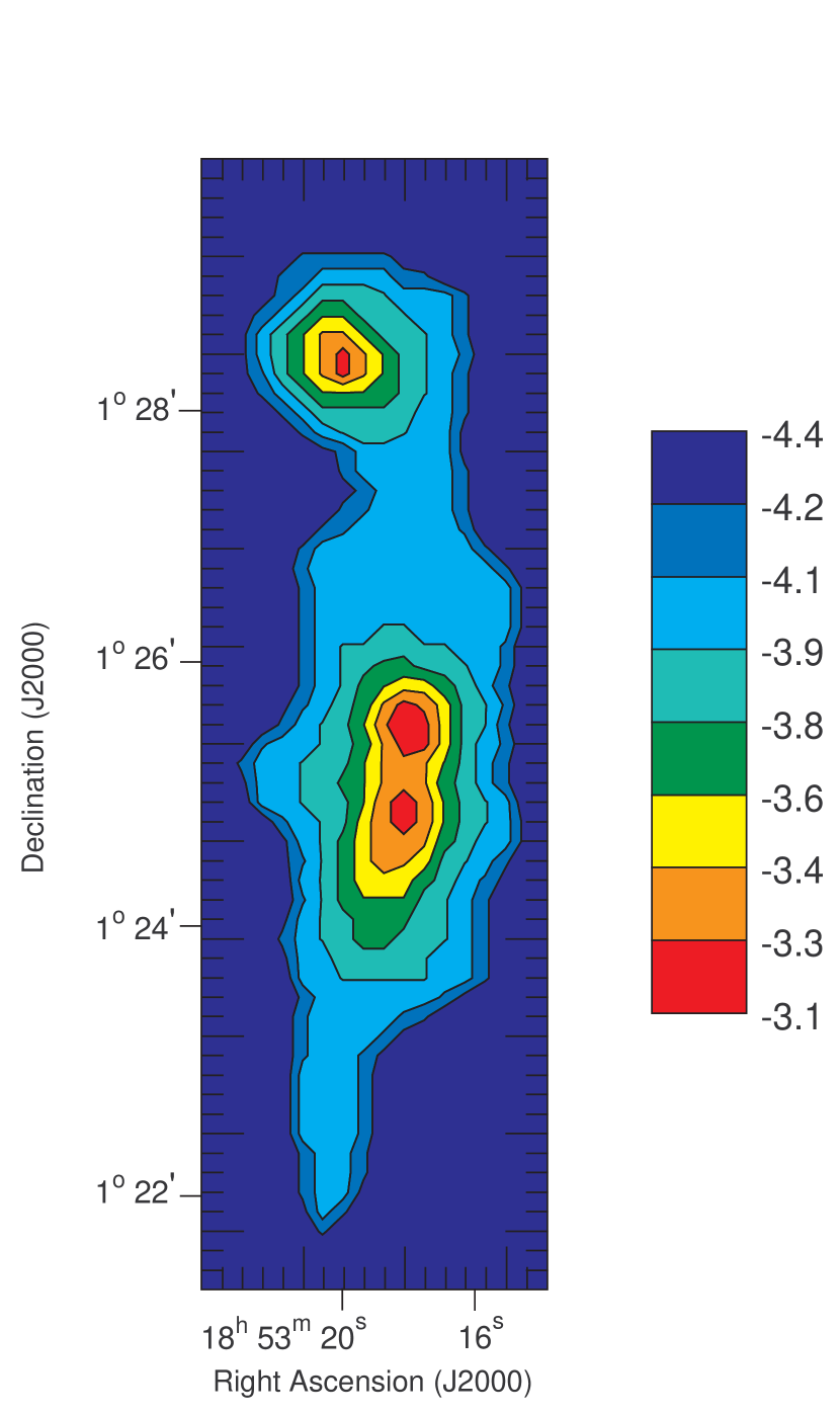
Figure 1: The contour color-fill for the logarithm of mean number density of ions, $\bar{n}_{i}$, in the unit of $\mathrm{cm}^{-3}$. The contours represent the isodensity points on the plane-of-sky and the faraway contour represents the periphery of the G34.

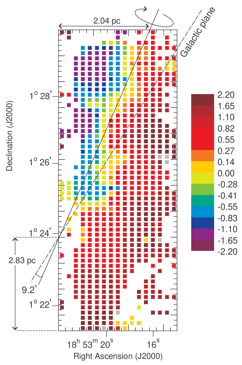
Figure 2: The color-pixel-map of the line-of-sight centroid velocity, relative to the median, in the unit of $\mathrm{km}\,\mathrm{s}^{-1}$. Pixels with a relative velocity of approximately zero (median value) are shown with a solid hypothetical line, which represents the axis of rotation, and has an approximate angle of $9.2^{\circ}$ to the Galactic plane. We do not have enough information about the line-of-sight centroid velocity at the boundaries of G34, and therefore these pixels are shown in white color.

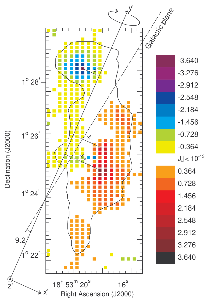
Figure 3: The color-pixel-map of the component of current density along the line-of-sight in the unit of $10^{-12}\,\mathrm{esu}\,\mathrm{s}^{-1}\,\mathrm{cm}^{-2}$. The contour represents the periphery of G34 and the outer pixels are not significant. The Galactic plane is shown by the dashed line. We choose the $x^{\prime}y^{\prime}z^{\prime}$ coordinate system so that the $z^{\prime}$-axis is in the line-of-sight and the $y^{\prime}$-axis coincides on the rotation axis, which has angle $9.2^{\circ}$ concerning the Galactic plane. The distances from the center of the clumps MM1, MM2, and MM3 to the rotation axis are indicated by $x^{\prime}_{1}$, $x^{\prime}_{2}$, and $x^{\prime}_{3}$, respectively.

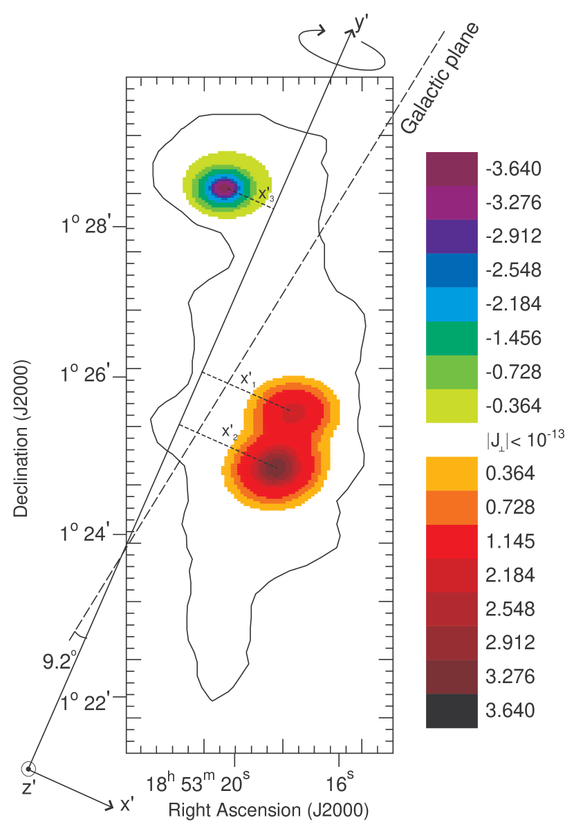
Figure 4: The same as Fig. 3 but with the mathematical model (4) and more pixels ($85\times 290$).

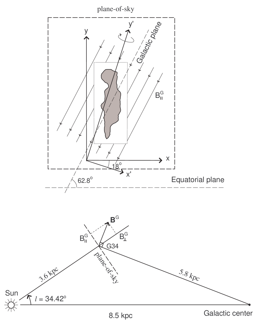
Figure 5: Lower panel: the location of IRDC G34 on the Galactic plane and the components of the Galactic magnetic field in this region. Upper panel: the apparent view of G34 on the plane-of-sky. In the upper panel, the equatorial and Galactic planes are shown as dashed lines, and the Galactic magnetic field component on the plane-of-sky around the G34 is shown uniformly and parallel to the Galactic plane. The primed coordinate system is chosen so that $y^{\prime}$ corresponds to the rotation axis and $z^{\prime}$ is in the line-of-sight. The $xyz$ coordinate system is obtained from rotation of the $x^{\prime}y^{\prime}z^{\prime}$ coordinate around the $z^{\prime}$-axis so that the $x$-axis is parallel to the equatorial plane.

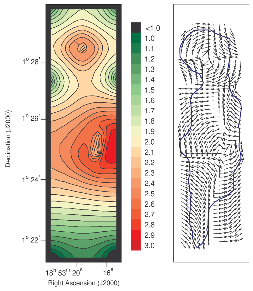
Figure 6: The contour color-fill of the logarithm of magnetic field strengths of G34 on the plane-of-sky in the unit of $\mu\mathrm{G}$ (left panel), and magnetic field orientations which are depicted by unit vectors (right panel).

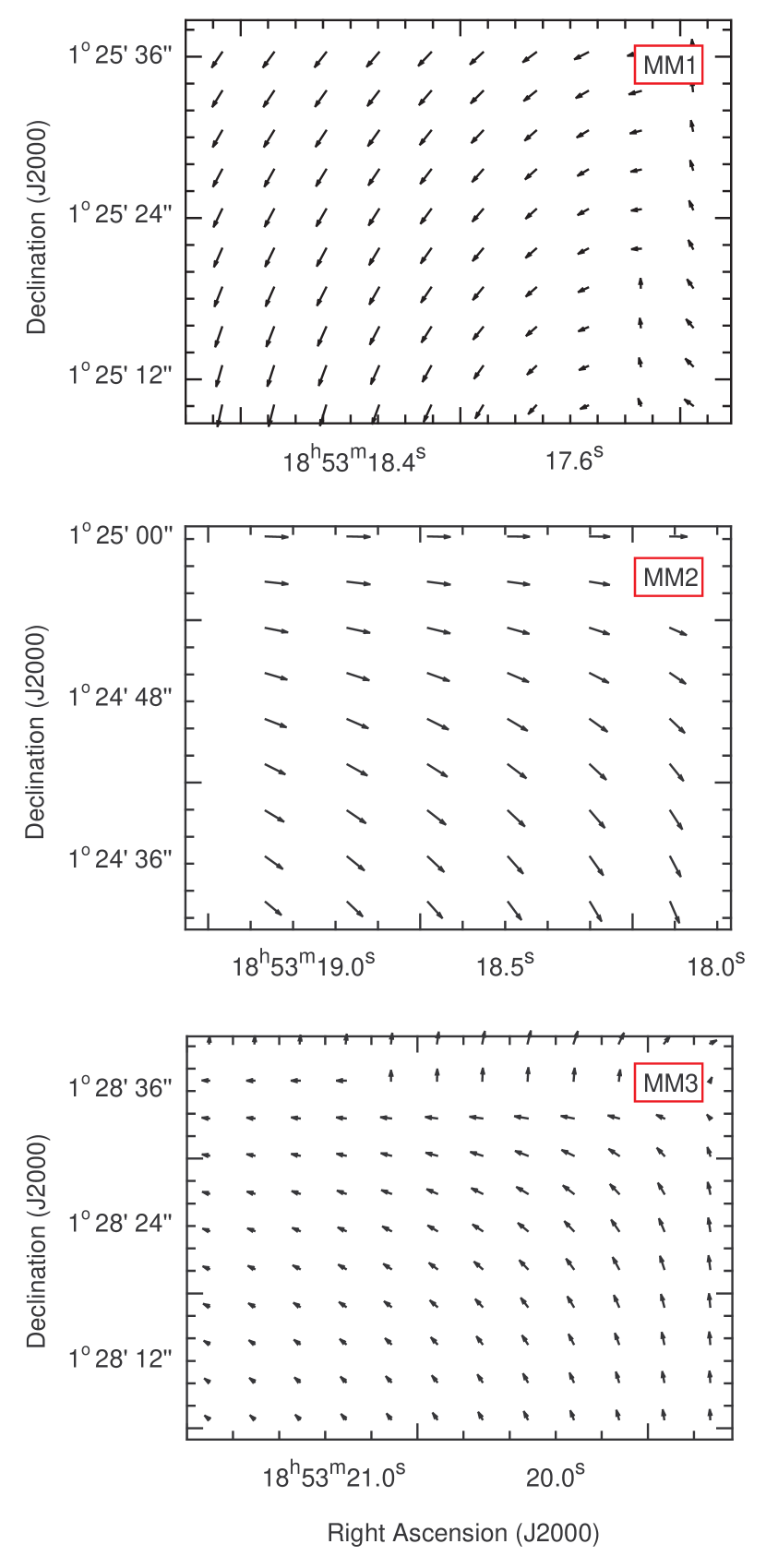
Figure 7: The vector-plot of plane-of-sky magnetic fields of clumps MM1, MM2 and MM3.

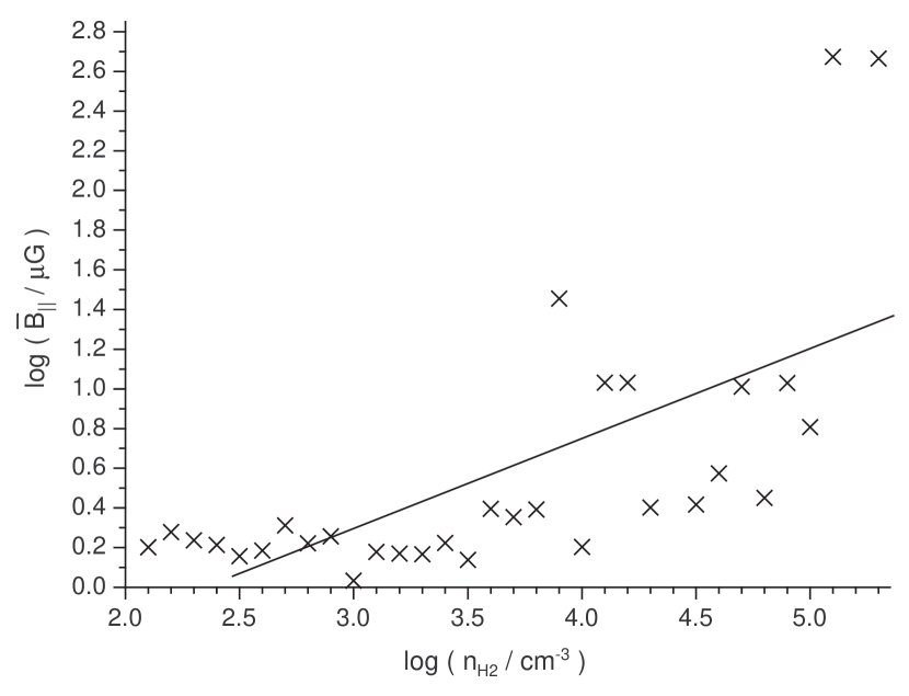
Figure 8: The logarithmic plot of the mean magnetic field versus $\mathrm{H}_{2}$ number density. The fitted straight-line indicates the relation $\bar{B}_{\parallel}\propto n_{\mathrm{H}_{2}}^{\eta}$ with power $\eta=0.45\pm 0.08$.

References

- (1) Adams J.C., Swarztrauber P.N., Sweet R., 2016, ascl:1609.004
- (2) Añez-López N., 2020, A&A, 644, 52
- (3) Arzoumanian D., Shimajiri Y., Inutsuka S., Inoue T., Tachihara K., 2018, PASJ, 70, 96
- (4) Ballesteros-Paredes J. et al., 2020, Space Science Reviews, 216, 76
- (5) Beuther H. et al., 2017, ApJ, 836, 199
- (6) Carey S.J., Clark F.O., Egan M.P., Price S.D., Shipman R.F., Kuchar T.A., 1998, ApJ, 508, 721
- (7) Carlqvist P., Gahm G.F., 1992, IEEE Transactions on Plasma Science, 20, 867
- (8) Crutcher R.M., 2012, ARA&A, 50, 29
- (9) Dirienzo W.J., Brogan C., Indebetouw R., Chandler C.J., Friesen R.K., Devine K.E., 2015, AJ, 150, 159
- (10) Egan M.P., Shipman R.F., Price S.D., Carey S.J., Clark F.O., Cohen M., 1998, ApJ, 494, 199
- (11) Heiles C., 1996, ApJ, 462, 316
- (12) Hennebelle P., Inutsuka S., 2019, FrASS, 6, 5
- (13) Hoq S., Clemens D.P., Guzmán A.E., Cashman L.R., 2017, ApJ, 836, 199
- (14) Hull C.L.H., 2014, ApJS, 213, 13
- (15) Inoue T., Hennebelle P., Fukui Y., Matsumoto T., Iwasaki K., Inutsuka S., 2018, PASJ, 70, 53
- (16) Isequilla N.L., Ortega M.E., Areal M.B., Paron S., 2021, A&A, 649, 139
- (17) Jansson R., Farrar G.R., 2012, ApJ, 757, 14
- (18) Jones T.J., Gordon M., Shenoy D., Gehrz R.D., Vaillancourt J.E., Krejny M., 2016, AJ, 151, 156
- (19) Juvela M. et al., 2018, A&A, 620, 26
- (20) Liu H., Sanhueza P., Liu T., Zavagno A., Tang X., Wu Y., Zhang S., 2020, ApJ, 901, 31
- (21) Liu J., Zhang Q., Qiu K., Liu H.B., Pillai T., Girart J.M., Li Z., Wang K., 2020, ApJ, 895, 142
- (22) Mouschovias T.Ch., Ciolek G.E., 1999, in Lada C.J., Kylafis N.D., eds, The Origin of Stars and Planetary Systems. NATO ASI Series C, Kluwer Academic Publishers, p. 305
- (23) Mestel L., 1966, MNRAS, 133, 265
- (24) Perault M. et al., 1996, A&A, 315, 165
- (25) Planck Collaboration et al., 2015, A&A, 576, 104
- (26) Press W.H., Teukolsky S.A., Vetterling W.T., Flannery B.P., 1992, Numerical recipes in FORTRAN. The art of scientific computing. Cambridge University Press
- (27) Pshirkov M.S., Tinyakov P.G., Kronberg P.P., Newton-McGee K.J., 2011, ApJ, 738, 192
- (28) Rathborne J.M., Jackson J.M., Chambers E.T., Simon R., Shipman R., Frieswijk W., 2005, ApJ, 630, 81
- (29) Rathborne J.M., Jackson J.M., Simon R., 2006, ApJ, 641, 389
- (30) Sanhueza P., Garay G., Bronfman L., Mardones D., May J., Saito M., 2010, ApJ, 715, 18
- (31) Santos F.P., Busquet G., Franco G.A.P., Girart J.M., Zhang Q., 2016, ApJ, 832, 186
- (32) Shu F.H., 1992, The Physics of Astrophysics: Gas Dynamics, University Science Books
- (33) Soam A. et al., 2019, ApJ, 883, 95
- (34) Sparke L.S., Gallagher III J.S., 2007, Galaxies in the Universe: An Introduction. Second Edition. Cambridge University Press, Cambridge, UK
- (35) Tang Y., Koch P.M., Peretto N., Novak G., Duarte-Cabral A., Chapman N.L., Hsieh P., Yen H., 2019, ApJ, 878, 10
- (36) Thaddeus P., Turner B.E., 1975, ApJ, 201, 25
- (37) Womack M., Ziurys L.M., Wyckoff S., 1992, ApJ, 387, 417
- (38) Wurster J., 2016, PASA, 33, 41
- (39) Wurster J., 2021, MNRAS, 501, 5873
- (40) Zenko T., Nagata T., Kurita M., Kino M., Nishiyama S., Matsunaga N., Nakajima Y., 2020, PASJ, 72, 27
- (41) Zhang Q., 2014, ApJ, 792, 116