Incorporating Heterophily into Graph Neural Networks for Graph Classification

Abstract

Graph neural networks (GNNs) often assume strong homophily in graphs, seldom considering heterophily which means connected nodes tend to have different class labels and dissimilar features. In real-world scenarios, graphs may have nodes that exhibit both homophily and heterophily. Failing to generalize to this setting makes many GNNs underperform in graph classification. In this paper, we address this limitation by identifying two useful designs and develop a novel GNN architecture called IHGNN (Incorporating Heterophily into Graph Neural Networks). These designs include integration and separation of the ego- and neighbor-embeddings of nodes; and concatenation of all the node embeddings as the final graph-level readout function. In the first design, integration is combined with separation by an injective function which is the composition of the MLP and the concatenation function. The second design enables the graph-level readout function to differentiate between different node embeddings. As the functions used in both the designs are injective, IHGNN, while being simple, has an expressiveness as powerful as the 1-WL. We empirically validate IHGNN on various graph datasets and demonstrate that it achieves state-of-the-art performance on the graph classification task.

I Introduction

Graphs can encode and represent relational structures that appear in many domains and thus are widely used in the real-world applications. One of the major tasks in graph applications is to classify graphs into different categories. For example, in the pharmaceutical industry, the molecule-based drug discovery needs to search for similar molecules with increased efficacy and safety against a specific disease. In this case, molecules are represented as graphs, where nodes represent atoms, edges represent chemical bonds, and node labels represent the types of atoms. The graph classification problems have been studied by conventional methods such as graph kernels [1, 2, 3]. However, graph kernels are defined mainly on the frequency of the occurrences of hand-crafted graph substructures without any automated learning about the structure; they are not adaptable to different kinds of graphs with different characteristics. Recently, graph neural networks (GNNs) [4, 5, 6, 7] have received a lot of attention as they are effective on learning representations of nodes as well as graphs and solving supervised learning problems on graphs.

C(-[:180]F)*6(-C-C(-[:300]N(-[:0]O)(-[:240]O))-C(-[:0]F)-C-C-)

(a) A heteroaromatic nitro compound.

C(-[:180]N(-[:120]O)(-[:240]O))*6(-C-C(-[:300]N(-[:0]O)(-[:240]O))-C(-[:0]Cl)-C-C-)

(b) A mutagenic aromatic nitro compound.

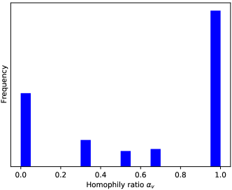
(c) The histogram of the homophily ratio of all the nodes.

Figure 1: (a) and (b) denote the graph structures of two different chemical compounds in the MUTAG [8, 9] dataset. These two chemical compounds have different mutagenic effect on a bacterium. The graph classification task aims to classify these chemical compounds by considering the atoms and their connection patterns (graph structures). Explicit hydrogen atoms have been removed. The labels of nodes represent the types of atoms, i.e., C (Carbon), N (Nitrogen), F (Fluorine), O (Oxygen), and Cl (Chlorine). (c) shows the homophily ratio $\alpha_{v}$ of all the nodes in this dataset.

GNNs broadly follow an iterative message passing [5] scheme, where node embeddings (i.e., messages) are aggregated and propagated through the graph structure, capturing the structural information. After $K$ iterations, the embedding of a node has aggregated the structural information within its $K$-hop neighborhood. The final node embeddings can be used directly for node classification or pooled for graph classification. Despite their great successes in many tasks [10] such as graph regression, graph classification, node classification, and link prediction, Xu et al. [11] have proved that the expressiveness of GNNs are at most as powerful as the first order Weisfeiler-Lehman graph isomorphism test (1-WL) [12] in distinguishing graph structures. It implies if two graphs that the 1-WL cannot distinguish as non-isomorphic, GNNs will also represent them with the same embedding (or representation). One way to improve the expressive power of GNNs is to focus on the message passing between higher-order relations in graphs [13, 14]. For instance, $k$-GNNs [13] uses message passing between one-, two-, and three-order node tuples hierarchically so as to reaching the 3-WL expressive power. PPGNs [14] is built on the $k$-order invariant and equivariant GNNs [15], of which the reduced 2-order has an equivalent expressive power to the 3-WL.

Theoretically, these models such as $k$-GNNs and PPGNs are more expressive than the GNNs that are at most as powerful as the 1-WL. However, more expressive power does not always induce higher generalization ability [16]. The higher-order relations and non-local message passing used in these models make them not only computationally expensive in large graphs, but also violate the locality principle [17]. This might be the reason why these models with higher expressive power cannot outperform the GNNs whose expressiveness is at most as powerful as the 1-WL on many tasks, as reported in [10].

Additionally, most of these models assume strong homophily in graphs, seldom considering heterophily. Homophily means the connected nodes tend to have the same class label and similar features while heterophily means the connected nodes tend to have different class labels and dissimilar features. In the real world, nodes in graphs may have both homophily and heterophily. For example, Figure 1(a) and (b) show two chemical compounds from the MUTAG [8, 9] dataset, which contains 188 chemical compounds that belong to two classes. We observe that the varying kinds and numbers of the atoms and their different connection patterns (graph structures) make the functions of these two chemical compounds different. Figure 1(c) demonstrates the histogram of the homophily ratio (Please see the definition in Section II-A.) of all the nodes in this dataset. The larger the homophily ratio of a node, the more number of neighboring nodes have the same class label. This is evident that both homophily and heterophily exist in molecules. Thus, considering only homophily might lead to weaker performance of GNNs as can be seen in Section IV.

To mitigate the above problems, in this paper, we investigate the expressive power of GNNs by considering both homophily and heterophily in their designs and develop a novel graph neural network model called IHGNN (Incorporating Heterophily into Graph Neural Networks) whose expressiveness is as powerful as the 1-WL. While the expressiveness of IHGNN is not as powerful as the 3-WL, it outperforms the 3-WL equivalent GNNs on the task of graph classification on many benchmark datasets. Our main contributions can be summarized as follows:

• We propose to use both the integration and separation of the ego- and neighbor-embeddings of nodes in the $\mbox{COMBINE}(\cdot)$ operator (formalized in Eqn. (3) in Section II-B) of GNNs. The integration of the ego- and neighbor-embeddings of nodes is effective in graphs that have high homophily ratio while the separation of the ego- and neighbor-embeddings of nodes is effective in graphs that have low homophily ratio. By considering both of these, GNNs are adaptable to different graphs with varying homophily ratio.

• We propose to use the composition of the Multi-layer Perceptrons (MLP) and the concatenation function as the injective function in the $\mbox{COMBINE}(\cdot)$ operator of GNNs so that two graphs the 1-WL decides as non-isomorphic will be projected to different embeddings by GNNs.

• We propose an injective graph-level readout function that discerns each node embedding, i.e., the embeddings of nodes with different homophily ratio are not mixed together. This is achieved by aligning nodes from different graphs in the same order as indicated by the continuous 1-WL colors (the node embeddings in the last layer).

• We develop a new GNN model called IHGNN that adopts all the above designs, which make its expressiveness as powerful as the 1-WL. Empirical results show that IHGNN outperforms other state-of-the-art GNNs on various graph datasets in terms of classification accuracy.

The remainder of the paper is organized as follows: Section 2 describes the preliminaries. Section 3 introduces our approach IHGNN which includes the integration and separation of ego- and neighbor-embeddings of nodes and the concatenation of all the node embeddings as the final graph-level readout function. Using benchmark datasets, Section 4 compares IHGNN with several existing GNNs. Section 5 discusses related work and Section 6 concludes the paper.

II Preliminaries

II-A Notations and Definitions

We begin with the notations and definitions used in this paper. We consider an undirected labeled graph $\mathcal{G}=(\mathcal{V},\mathcal{E},l)$, where $\mathcal{V}=\left\{v_{1},\ldots,v_{n}\right\}$ is a set of vertices (nodes), $\mathcal{E}$ is a set of edges, and $l:\mathcal{V}\rightarrow\Sigma$ is a function that assigns labels from a set of positive integers $\Sigma$ to nodes. Without loss of generality, $\lvert\Sigma\rvert\leq|\mathcal{V}|$. An edge $e$ is denoted by two nodes $uv$ that are connected to it. The adjacency matrix of nodes is denoted by $\mathbf{A}\in\mathbb{R}^{n\times n}$ with $a_{i,j}=a_{j,i},a_{i,i}=0$. The degree matrix $\mathbf{D}$ is a diagonal matrix associated with $\mathbf{A}$ with $d_{i,i}=\sum_{j}a_{i,j}$. For a graph with self-loops on each node, its adjacency matrix is defined as $\mathbf{\widetilde{A}}=\mathbf{A}+\mathbf{I}$. And the corresponding degree matrix is $\mathbf{\widetilde{D}}$. The indicator function is denoted by $\mathds{1}(x)$. $\mathcal{N}_{v}$ denotes the one-hop neighbors of node $v$ (excluding itself). $\cdot\parallel\cdot$ is the concatenation operator. We represent the set of feature vectors of a node’s neighbors as a multiset $\left\{\mskip-7.0mu\left\{\cdot\right\}\mskip-7.0mu\right\}$ (a set with possibly the same element multiple times).

In this paper, our goal is to improve the expressive power and performance of GNNs by considering both homophily and heterophily. Let us first define the homophily ratio $\alpha_{v}$ of a node $v$ in a graph:

$$\alpha_{v}=\frac{\sum_{u\in\mathcal{N}_{v}}\mathds{1}\left(\mbox{label}(u)=\mbox{label}(v)\right)}{\left|\mathcal{N}_{v}\right|}$$ (1)

we can see that the larger the $\alpha_{v}$ value, the more number of neighboring nodes have the same label as node $v$. For the whole graph, we define its homophily ratio $\beta$ as follows:

$$\beta=\frac{1}{\left|\mathcal{V}\right|}\sum_{v\in\mathcal{V}}\alpha_{v}$$ (2)

the larger the $\beta$ value, the stronger the homophily of the graph, i.e., the more number of nodes have the same label.

II-B Graph Neural Networks

Graph Neural Networks (GNNs) use the graph structure and the node features to learn the embeddings or representations of nodes or the entire graph. A majority of GNNs [5, 6, 7] follow the message passing strategy, i.e., iteratively updating the embedding of a node by aggregating those of its neighboring nodes. After $k$ iterations, the embedding of a node captures information from both the graph structure and all its neighbors’ embeddings in its $k$-hop neighborhood. In the $k$-th layer, GNNs have two operators: $\mbox{AGGREGATE}^{(k)}(\cdot)$ and $\mbox{COMBINE}^{(k)}(\cdot)$, whose definitions are given as follows:

$$\mathbf{h}_{\mathcal{N}_{v}}^{(k)} =\mbox{AGGREGATE}^{(k)}\left(\left\{\mskip-7.0mu\left\{\mathbf{h}_{u}^{(k-1)},\forall u\in\mathcal{N}_{v}\right\}\mskip-7.0mu\right\}\right)$$ (3)

$$\mathbf{h}_{v}^{(k)} =\mbox{COMBINE}^{(k)}\left(\mathbf{h}_{v}^{(k-1)},\mathbf{h}_{\mathcal{N}_{v}}^{(k)}\right)$$

where $\mathbf{h}_{v}^{(k)}$ is the embedding of node $v$ at the $k$-th layer. Usually, $\mathbf{h}_{v}^{(0)}$ is initialized as the node feature vector $\mathbf{x}_{v}$ (one-hot encoding of the node label or the continuous attributes of node). $\mathbf{h}_{\mathcal{N}_{v}}^{(k)}$ is the aggregation of the embeddings of neighboring nodes of $v$.

There are different functions that are used in $\mbox{AGGREGATE}^{(k)}(\cdot)$ and $\mbox{COMBINE}^{(k)}(\cdot)$ in GNNs. For example, in GCN [7], $\mbox{AGGREGATE}^{(k)}(\cdot)$ and $\mbox{COMBINE}^{(k)}(\cdot)$ have the following forms:

$$\mathbf{h}_{\mathcal{N}_{v}}^{(k)} =\sum_{u\in\mathcal{N}_{v}}\left(\widetilde{d}_{v}\widetilde{d}_{u}\right)^{-1/2}\mathbf{h}_{u}^{(k-1)}$$ (4)

$$\mathbf{h}_{v}^{(k)} =\mathop{\mathrm{ReLU}}\left(\mathbf{W}^{(k)}\left(\widetilde{d}_{v}^{-1}\mathbf{h}_{v}^{(k-1)}+\mathbf{h}_{\mathcal{N}_{v}}^{(k)}\right)\right)$$

where $\widetilde{d}_{v}$ is the degree of node $v$ (including itself) and $\mathbf{W}^{(k)}$ is the learning weights of the $k$-th layer.

After learning node embeddings in the $k$-th layer, GNNs perform a readout function to aggregate all the node embeddings to generate an embedding for the entire graph. It can be computed as follows:

$$\mathbf{h}_{\mathcal{G}}=\mathop{\mathrm{READOUT}}\left(\left\{\mskip-7.0mu\left\{\mathbf{h}_{v}^{(k)},\forall v\in\mathcal{G}\right\}\mskip-7.0mu\right\}\right)$$ (5)

where $\mathop{\mathrm{READOUT}}(\cdot)$ should be a permutation- and size-invariant function of node embeddings such as summation or other advanced techniques, e.g., DeepSets [18].

III Our Proposed Method (IHGNN)

One of the major motivations of our proposed method is to consider the fact that the heterophily property exists in real-world graphs. In molecules (e.g., two chemical compounds from the MUTAG dataset in Section I), atoms tend to form chemical bonds with both the same and different kinds of atoms. Thus, nodes in such molecule graphs have both homophily and heterophily. For graphs with varying node homophily ratio, considering only one mode might limit the expressive power of GNNs as well as the performance in graph classification. So in this paper, we propose two novel designs besides the skip-connection used in JK-Nets [19] and GIN [11] to improve the expressive power of GNNs by considering both the modes. To the best of our knowledge, we are the first to consider both homophily and heterophily in the design of GNN architectures for graph classification. Next, we describe our designs in more details.

III-A Integration and Separation of Ego- and Neighbor-embeddings

GIN [11] argues that the sum aggregator has more expressive power than the mean and max aggregators over a multiset. Here, we also use the sum aggregator as our aggregation function, $\mbox{AGGREGATE}^{(k)}(\cdot)$:

$$\mathbf{h}_{\mathcal{N}_{v}}^{(k)}=\sum_{u\in\mathcal{N}_{v}}\mathbf{h}_{u}^{(k-1)}$$ (6)

To consider both the integration and separation of the ego- and neighbor-embeddings of nodes, we develop $\mbox{COMBINE}^{(k)}(\cdot)$ as follows:

$$\mathbf{h}_{v}^{(k)}=\mbox{MLP}^{(k)}\left(\mathbf{h}_{v}^{(k-1)}\parallel\mathbf{h}_{\mathcal{N}_{v}}^{(k)}\parallel\left(\mathbf{h}_{v}^{(k-1)}+\mathbf{h}_{\mathcal{N}_{v}}^{(k)}\right)\right)$$ (7)

where $\mbox{MLP}^{(k)}$ denotes the Multi-layer Perceptrons for the $k$-th layer. We concatenate each node’s ego-embedding, neighbor-embedding, and their summation, and use MLP to generate a new ego-embedding for each node.

III-A1 Relation to Weisfeiler-Lehman Isomorphism Test

Weisfeiler-Lehman isomorphism test (WL) [12] decides whether or not two graphs are isomorphic. Formally, we define graph isomorphism [20] as follows:

Definition 1 (Graph Isomorphism).

Two undirected labeled graphs $\mathcal{G}_{1}=(\mathcal{V}_{1},\mathcal{E}_{1},l_{1})$ and $\mathcal{G}_{2}=(\mathcal{V}_{2},\mathcal{E}_{2},l_{2})$ are isomorphic (denoted by $\mathcal{G}_{1}\simeq\mathcal{G}_{2}$) if there is a bijection $\varphi:\mathcal{V}_{1}\rightarrow\mathcal{V}_{2}$, (1) such that for any two nodes $u,v\in\mathcal{V}_{1}$, there is an edge $uv$ if and only if there is an edge $\varphi(u)\varphi(v)$ in $\mathcal{G}_{2}$; (2) and such that $l_{1}(v)=l_{2}(\varphi(v))$.

WL belongs to the family of color refinement algorithms that iteratively update node colors (labels) until reaching the fixed number of iterations, or the node label sets of two graphs are different (i.e., these two graphs are non-isomorphic). Figure 2 shows one iteration of the first order Weisfeiler-Lehman isomorphism test (1-WL) for graphs $\mathcal{G}_{1}$ and $\mathcal{G}_{2}$. For each node in these two graphs, the 1-WL first sorts the labels of its neighboring nodes in ascending order and then concatenates them as a string. Second, the 1-WL concatenates the label of this node and the concatenated labels of its neighboring nodes and uses a hash function to project the label string to a new integer label. The $\mbox{AGGREGATE}^{(k)}(\cdot)$ and $\mbox{COMBINE}^{(k)}(\cdot)$ can be written as follows:

$$s_{\mathcal{N}_{v}}^{(k)}=\parallel_{u\in\mathcal{N}_{v}}l^{(k-1)}(u)$$ (8)

$$l_{v}^{(k)}=g\left(l^{(k-1)}(v)\parallel s_{\mathcal{N}_{v}}^{(k)}\right)$$ (9)

where $l^{(k)}(v)$ is the label of node $v$ at the $k$-th iteration, $s_{\mathcal{N}_{v}}^{(k)}$ is a string of the concatenated labels of neighboring nodes of node $v$, and $g(\cdot)$ is a hash function. What makes the 1-WL so powerful is that the concatenation and the hash function $g(\cdot)$ are injective functions that project different multisets to different labels.

In this paper, we use one-hot encoding for each node label. Compared with Eqn. (8), the concatenation is replaced with the summation in Eqn. (6). Compared with Eqn. (9), the injective hash function $g(\cdot)$ is replaced with the MLP in Eqn. (7), because MLP can model and learn injective function thanks to the universal approximation theorem [21, 22]. In addition, we also concatenate the summation of the ego- and neighbor-embeddings of nodes, which is not feasible in Eqn. (9) because strings have no mathematical summation operation.

(a) $\mathcal{G}_{1}$

(b) $\mathcal{G}_{2}$

(c) $\mathcal{G}_{1}$: Label Concatenation

(d) $\mathcal{G}_{2}$:Label Concatenation

(e) $\mathcal{G}_{1}$: Label Hashing

(f) $\mathcal{G}_{2}$: Label Hashing

Figure 2: Illustration of one iteration of the first order Weisfeiler-Lehman isomorphism test (1-WL) for graphs. (c) and (d) show that for each node in $\mathcal{G}_{1}$ and $\mathcal{G}_{2}$, 1-WL concatenates its label and the labels of its neighboring nodes as a string. (e) and (f) show that 1-WL uses an injective hash function to project the label string to a new integer label. For (a) and (b), $\Sigma=\{1,2,3,4\}$. For (e) and (f), $\Sigma=\{5,6,7,8,9,10,11,12,13,14\}$.

III-B Graph-level Readout Function

In the previous section, we have obtained the representation or embedding for each node (Eqn. (7)). Each node embedding learned in each layer/iteration corresponds to the subtree structure of height one rooted at this node. With the increasing number of iterations, the node embedding becomes more global. In each iteration, the node embedding captures the graph structure information at different levels of granularities. As indicated by Zhu et al. [23], in graphs with low homophily ratio, the node label distribution contains more information at the higher orders of the adjacency matrix than the lower orders of the adjacency matrix. Therefore, the concatenation of the intermediate node embeddings from different layers/iterations increases the expressive power of GNNs, which has been proved theoretically in [23]. This skip-connection strategy is also used in JK-Nets [19] and GIN [11]. For each node $v$, its final embedding is as follows:

$$\mathbf{h}_{v}=\mathbf{h}_{v}^{(1)}\parallel\mathbf{h}_{v}^{(2)}\parallel\cdots\parallel\mathbf{h}_{v}^{(K)}$$ (10)

where $K$ is the number of layers/iterations.

Many variants of GNNs use the summation as the final graph-level readout function. However, as for graphs with varying node homophily ratio, the summation of all the node embeddings ignores the characteristic of each node, which makes nodes with low homophily ratio indistinguishable from those with high homophily ratio. Intuitively, this decreases the expressive power of GNNs. To mitigate this problem, we propose to concatenate all the node embeddings. However, the concatenation function does not satisfy the conditions of the graph-level readout function, i.e., permutation-invariance and size-invariance.

Satisfying permutation-invariance: To solve the problem of permutation-invariance, we propose to align nodes such that nodes from different graphs are sorted and aligned in the same order, which is consistent across different graphs. Now the ordering in which we sort the nodes so that they are aligned across different graphs becomes important. We adopt the 1-WL to sort nodes, because the final 1-WL colors define an ordering based on the node structural identity and this ordering is consistent across different graphs. For example, in Figure 2(e) and (f), the 1-WL will sort the nodes in $\mathcal{G}_{1}$ in an order of $7,7,9,11,12,13$ and sort the nodes in $\mathcal{G}_{2}$ in an order of $5,6,8,10,12,14$. The two nodes with label $12$ in $\mathcal{G}_{1}$ and $\mathcal{G}_{2}$ have the same position in the two orders. Note that the $\mbox{AGGREGATE}^{(k)}(\cdot)$ and $\mbox{COMBINE}^{(k)}(\cdot)$ operators in GNNs are the continuous versions of the aggregate and hash operators in the 1-WL. We sort nodes in each graph by their final embeddings, which can be considered as the continuous 1-WL colors.

Satisfying size-invariance: To solve the problem of size-invariance, we use the size (say $m$) of the graph that has the largest number of nodes as the common size. For graphs whose sizes are less than $m$, we concatenate them with dummy nodes to make their sizes equal to $m$. The features of the dummy nodes are set to zero vectors so that they do not contribute in learning the associated parameters. After aligning the nodes from different graphs and making different graphs of the same size, the graph-level readout function is given as follows:

$$\mathbf{h}_{\mathcal{G}}=\mathbf{h}_{\sigma_{v_{1}}}\parallel\mathbf{h}_{\sigma_{v_{2}}}\parallel\cdots\parallel\mathbf{h}_{\sigma_{v_{m-w}}}\parallel\underbrace{\mathbf{0}\parallel\cdots\parallel\mathbf{0}}_{w}$$ (11)

where $m-w$ is the number of nodes in a graph that does not have the largest node number and $\sigma_{v_{1}},\sigma_{v_{2}},\ldots,\sigma_{v_{m-w}}$ is an order on nodes defined by the continuous 1-WL colors. Finally, we input $\mathbf{h}_{\mathcal{G}}$ into an MLP followed by a softmax layer for graph classificaion.

III-C Discussion on the Expressive Power of IHGNN

In this section, we analyze the expressive power of IHGNN. We show that the expressiveness of our model IHGNN is as powerful as the 1-WL. For our analysis, we adopt the proven result in GIN [11] as follows:

Theorem 1.

[11] Let $\mathcal{A}:\mathcal{G}\rightarrow\mathbb{R}^{d}$ be a GNN. With a sufficient number of GNN layers, $\mathcal{A}$ maps any graphs $\mathcal{G}_{1}$ and $\mathcal{G}_{2}$ that the Weisfeiler-Lehman isomorphism test decides as non-isomorphic, to different embeddings if the following conditions hold:

• $\mathcal{A}$ aggregates and updates node features iteratively with:

  $$\mathbf{h}_{v}^{(k)}=\phi\left(\mathbf{h}_{v}^{(k-1)},f\left(\left\{\mskip-7.0mu\left\{\mathbf{h}_{u}^{(k-1)}:u\in\mathcal{N}_{v}\right\}\mskip-7.0mu\right\}\right)\right)$$ (12)

  where the functions $f(\cdot)$, which operates on the multisets, and $\phi(\cdot)$ are injective.

• $\mathcal{A}$’s graph-level readout function, which operates on the multiset of node features $\left\{\mskip-7.0mu\left\{\mathbf{h}_{v}^{(k)},\forall v\in\mathcal{G}\right\}\mskip-7.0mu\right\}$, is injective.

Our designs in Eqn. (6), Eqn. (7), Eqn. (10), and Eqn. (11) satisfy all the conditions in Theorem 1. We use summation, which has been proven to be injective in GIN [11], to model $f(\cdot)$ in Eqn. (12). The function $\phi(\cdot)$ is modeled as the composition of the MLP and the concatenation function. Since the concatenation function is injective and the MLP can model and learn injective function, their composition $\phi(\cdot)$ is also injective. Thus, the expressiveness of our model IHGNN is as powerful as the 1-WL.

III-D Computational Complexity of IHGNN

The pseudo-code of IHGNN is given in Algorithm 1. Line 1 initializes the parameters of all the neural networks. At line 5, for each graph $\mathcal{G}$ in a batch of training data, we use an MLP to transform the one-hot encoding $\mathbf{X}\in\mathbb{R}^{n\times c}$ of node labels to the embeddings $\mathbf{H}^{(1)}\in\mathbb{R}^{n\times r}$, where $c$ is the number of classes, $r$ is the dimension of the embedding. Assume that every graph has the same number $n$ of nodes and the number of neurons of the hidden and output layers of MLP are equal. The time complexity of line 5 is $\mathcal{O}(n\cdot c\cdot r+n\cdot r\cdot r)$. Lines 6–7 update each node embedding iteratively by the $\mbox{AGGREGATE}^{(k)}(\cdot)$ and $\mbox{COMBINE}^{(k)}(\cdot)$ operators in Eqn. (6) and Eqn. (7). The time complexity is $\mathcal{O}\left(K\cdot\left(\mbox{vol}(\mathcal{G})\cdot r+n\cdot r^{2}\right)\right)$, where $\mbox{vol}(\mathcal{G})=\sum_{i}d_{i,i}$ is the volume of the graph $\mathcal{G}$. At line 8, we concatenate all the intermediate node embeddings. At line 9, we sort nodes in ascending order according to their continuous 1-WL colors. Since the node embedding vector (the continuous 1-WL color) in the last layer is of $r$ dimensions, we can sort nodes just using one dimension of their continuous 1-WL colors in order to make them aligned across different graphs. The time complexity is $\mathcal{O}(n\cdot\log(n))$. At line 10, we generate the graph embedding $\mathbf{h}_{\mathcal{G}}$ and input it into MLP for graph classification. The time complexity is $\mathcal{O}(n\cdot K\cdot r\cdot r^{\prime}+n\cdot r^{\prime}\cdot c)$, where $r^{\prime}$ is the number of neurons of the hidden layer of MLP, which is used for graph classification. Finally, Line 11 utilizes the back-propagation strategy to update the parameters of all the neural networks. Since $c\ll r$ and $r^{\prime}$ is in the same scale as $r$, the total time complexity of IHGNN in one epoch on a batch $b$ of graphs is bounded by $\mathcal{O}\left(b\cdot\left(n\cdot K\cdot r^{2}+\mbox{vol}(\mathcal{G})\cdot K\cdot r+n\cdot\log(n)\right)\right)$.

Input: A set of graphs $\{\mathcal{G}_{1},\mathcal{G}_{2},\ldots,\mathcal{G}_{n}\}$ and their corresponding labels $\mathcal{Y}=\{y_{1},y_{2},\ldots,y_{n}\}$, the number $K$ of layers, batch size $b$, the number of epochs $E$

Output: Classification accuracy

1 Initialize the parameters of all the neural networks;

2 while epoch $\leq E$ do

3       foreach batch of graphs $\{\mathcal{G}_{\gamma_{1}},\mathcal{G}_{\gamma_{2}},\ldots,\mathcal{G}_{\gamma_{b}}\}$ in the training data do

             /* $\gamma_{1},\gamma_{2},\ldots,\gamma_{b}$ denote the indexes in this batch of graphs */

4             foreach graph $\mathcal{G}$ in the batch  do

                   $\mathbf{H}^{(1)}\leftarrow\mbox{MLP}^{(1)}\left(\mathbf{X}\right)$;

                    /* Each row of $\mathbf{X}$ represents the one-hot encoding of each node label. */

5                   for $k\leftarrow 2$ to $K$ do

                         $\mathbf{H}^{(k)}\leftarrow\mathbf{H}^{(k-1)}\parallel\mathbf{A}\cdot\mathbf{H}^{(k-1)}\parallel\left(\mathbf{H}^{(k-1)}+\mathbf{A}\cdot\mathbf{H}^{(k-1)}\right)$;

                          /* $\mathbf{A}$ is the adjacency matrix of the graph $\mathcal{G}$. */

6                        

7                  $\mathbf{H}\leftarrow\mathbf{H}^{(1)}\parallel\mathbf{H}^{(2)}\parallel\cdots\parallel\mathbf{H}^{(K)}$;

8                   Sort nodes in ascending order according to the continuous 1-WL colors;

9                   Generate the graph embedding $\mathbf{h}_{\mathcal{G}}$ using Eqn. (11) and input it into MLP for graph classification;

10                  

11            Back-propagate to update the parameters of all the neural networks;

12            

13      

14return Classification accuracy;

Algorithm 1 IHGNN

IV Experimental Evaluation

IV-A Experimental Setup

We compare IHGNN with the following state-of-the-art graph neural networks:

1. GCN [7]: GCN uses a localized first-order approximation of spectral graph convolutions for scalable learning on graphs.

2. GraphSAGE [24]: GraphSAGE is inspired by the 1-WL, which separates the ego- and neighbor-embeddings of nodes.

3. DiffPool [25]: DiffPool is a differentiable graph pooling module that learns to pooling nodes in graphs hierarchically.

4. DGCNN [26]: DGCNN proposes a SortPooling layer to align nodes from different graphs for graph classification.

5. GIN [11]: GIN studies the expressive power of GNNs and proposes a GNN model that is as powerful as the 1-WL.

6. $k$-GNNs [13]: $k$-GNNs perform message passing directly between graph substructures rather than individual nodes so as to reaching the 3-WL expressive power.

7. PPGNs [14]: PPGNs is built on the $k$-order invariant and equivariant GNNs. Its expressiveness is as powerful as the 3-WL.

8. GNNML [16]: GNNML designs a GNN architecture that employs as many of the matrix operations in the MATLANG language as possible to reach an expressiveness as powerful as the 3-WL.

We perform ten-fold cross-validation and report the mean and standard deviation of classification accuracies. For each method, we train for 350 epochs using Adam [27] optimization method. For IHGNN, the batch size is selected from $\left\{32,128\right\}$. The number of layers is selected from $\left\{3,5\right\}$. The dropout ratio is set to 0.5, the number of neurons of the hidden and output layers of all the MLPs in the $\mbox{COMBINE}^{(k)}(\cdot)$ operator is set to 32, and the number of neurons of the hidden layer of the final MLP for graph classification is set to 128. Following GIN [11], the number of epochs is set as the one that has the best cross-validation accuracy averaged over the ten folds. For all the comparison methods, we set their hyperparameters according to their original papers.

We run all the experiments on a server with a dual-core Intel(R) Xeon(R) Silver 4110 CPU@2.10GHz, 128 GB memory, an Nvidia GeForce RTX 3090 GPU, and Ubuntu 18.04.1 LTS operating system. IHGNN is implemented with Pytorch. We make our code publicly available at Github.

IV-B Datasets

We adopt 14 benchmark graph datasets to evaluate each method. The statistics of datasets are shown in Table I and their characteristics are described as follows:

• Brain network dataset. KKI [28] is a brain network constructed from the whole brain functional resonance image (fMRI) atlas. Each node corresponds to a region of interest (ROI), and each edge represents the correlation relationship between two ROIs. KKI is constructed for the task of Attention Deficit Hyperactivity Disorder (ADHD) classification.

• Chemical compound datasets. The MUTAG [9] dataset consists of 188 chemical compounds that can be divided into two classes according to their mutagenic effect on a bacterium. The datasets BZR_MD, COX2_MD, DHFR, DHFR_MD are from [29]. These chemical compounds are represented by graphs, where edges represent the chemical bond types (single, double, triple or aromatic) and nodes represent atoms. Node labels indicate atom types. BZR is a dataset of ligands for the benzodiazepine receptor. COX2 consists of cyclooxygenase-2 inhibitors. DHFR has 756 inhibitors of dihydrofolate reductase. BZR_MD, COX2_MD, and DHFR_MD are derived from BZR, COX2, and DHFR, respectively, by removing explicit hydrogen atoms. The chemical compounds in the datasets BZR_MD, COX2_MD, and DHFR_MD are complete graphs. NCI1 [30] is a balanced subset of dataset of chemical compounds screened for activity against non-small cell lung cancer and ovarian cancer cell lines, respectively.

• Molecular compound datasets. The PTC [8] dataset consists of compounds labeled according to carcinogenicity on rodents divided into male mice (MM), male rats (MR), female mice (FM) and female rats (FR). The dataset PROTEINS  [31] consists of proteins where each protein is represented by a graph. In these graphs, nodes represent secondary structure elements and edges represent that two nodes are neighbors along the amino acid sequence or three-nearest neighbors to each other in space. The dataset DD [32] is a dataset of protein structures. Each protein is represented by a graph, in which the nodes are amino acids and two nodes are connected by an edge if they are less than six Ångstroms apart.

• Movie collaboration dataset. IMDB-MULTI is a dataset from [33], which contains movies of different actor/actress and genre information. For each collaboration graph, nodes represent actors/actresses. Edges denote that two actors/actresses appear in the same movie. The collaboration graphs are generated on Comedy, Romance, and Sci-Fi genres. For each actor/actress, a corresponding ego-network is derived and labeled with its genre.

TABLE I: Statistics of the benchmark datasets used in the experiments. N/A means the dataset does not have node labels. The column $\beta$ denotes the mean and standard deviation of the homophily ratio of each dataset.

Dataset	Size	Class #	Average node #	Average edge #	Node label #	$\beta$
KKI	83	2	26.96	48.42	190	0$\pm$0
MUTAG	188	2	17.93	19.79	7	0.62$\pm$0.14
BZR_MD	306	2	21.30	225.06	8	0.60$\pm$0.08
COX2_MD	303	2	26.28	335.12	7	0.51$\pm$0.09
DHFR	467	2	42.43	44.54	9	0.57$\pm$0.12
DHFR_MD	393	2	23.87	283.01	7	0.51$\pm$0.07
NCI1	4110	2	17.93	19.79	37	0.75$\pm$0.10
PTC_MM	336	2	13.97	14.32	20	0.50$\pm$0.23
PTC_MR	344	2	14.29	14.69	18	0.51$\pm$0.22
PTC_FM	349	2	14.11	14.48	18	0.50$\pm$0.22
PTC_FR	351	2	14.56	15.00	19	0.51$\pm$0.22
PROTEINS	1113	2	39.06	72.82	3	0.83$\pm$0.12
DD	1178	2	284.32	715.66	82	0.06$\pm$0.02
IMDB-MULTI	1500	3	13.00	65.94	N/A	0.81$\pm$0.23

IV-C Results

IV-C1 Classification Accuracy

We compare the classification accuracy of IHGNN with other GNNs on the 14 benchmark datasets in Table II. If a comparison method has reported the classification accuracy on a specific dataset, we adopt the result from the original paper. Otherwise, we run the original code to get the results.

We observe in Table II that IHGNN achieves the best results on nine out of 14 datasets. Although $k$-GNNs, PPGNs, and GNNML have an expressiveness as powerful as the 3-WL, they are outperformed by IHGNN, which has an expressiveness as powerful as the 1-WL, on nine datasets. On other five datasets, the best results are achieved by GraphSAGE, DiffPool, PPGNs, and GNNML. However, the performance gap between IHGNN and these four methods are not significant.

On the KKI dataset, IHGNN outperforms all the baselines. It has a gain of 2.0% over the runner-up method $k$-GNNs and a gain of 15.5% over the worst method DGCNN. Figure 3 shows the histogram of the homophily ratio $\alpha_{v}$ of nodes in each dataset. All the nodes in the KKI dataset have the same homophily ratio of value zero, which means the KKI dataset is heterophilous. All the comparison methods except GraphSAGE do not consider the separation of the ego- and neighbor-embeddings of nodes, which leads to inferior performance. This phenomenon also happens on other datasets, such as BZR_MD, COX2_MD, and DHFR_MD, with a bi-modal distribution (having two modes/peaks) of node homophily ratio. So, our designs of the integration and separation of the ego- and neighbor-embeddings of nodes and the graph-level readout function are effective on datasets with a bi-modal distribution of node homophily ratio.

For the NCI1 and PROTEINS datasets, many of their nodes have a high homophily ratio. IHGNN is outperformed by PPGNs on these two datasets. For dataset DD, many of its nodes have a low homophily ratio. IHGNN is superior to all the comparison methods except DiffPool. GraphSAGE also separates the ego- and neighbor-embeddings of nodes. But it does not consider the integration of the ego- and neighbor-embeddings of nodes. For the graph-level readout function, it uses the summation rather than the concatenation of all the node embeddings. From Table II, it is evident that IHGNN is significantly better than GraphSAGE on most of the datasets except PTC_FR.

Since the IMDB-MULTI dataset does not have node labels, we use node degrees as a proxy for their labels and plot the histogram of the node homophily ratio. Considering both the histogram of the node homophily ratio and the high homophily ratio $\beta$ of the dataset shown in Table I, we conclude that most of the nodes in IMDB-MULTI have the same degree. The performance of IHGNN is surprisingly slightly better than GIN on IMDB-MULTI.

TABLE II: Comparison of classification accuracy (mean $\pm$ standard deviation) of IHGNN to other GNNs on the benchmark datasets. N/A means the results are not reproducible because of existing bugs in the codes. ^† means the results are adopted from the original papers.

Dataset	IHGNN	GCN	GraphSAGE	DiffPool	DGCNN	GIN	$k$-GNNs	PPGNs	GNNML
KKI	65.0$\pm$13.5	59.9$\pm$20.8	61.5$\pm$16.9	58.8$\pm$13.8	56.3$\pm$18.8	60.3$\pm$12.5	63.7$\pm$16.3	57.5$\pm$12.1	61.3$\pm$16.3
MUTAG	90.6$\pm$8.3	83.0$\pm$7.1	83.0$\pm$5.6	86.7$\pm$7.3	85.8$\pm$1.7†	90.0$\pm$8.8†	86.1†	90.6$\pm$8.7†	90.9$\pm$5.5†
BZR_MD	75.7$\pm$6.2	70.9$\pm$8.6	72.2$\pm$8.1	71.2$\pm$6.8	64.7$\pm$9.3	70.5$\pm$8.0	72.0$\pm$8.5	70.7$\pm$7.8	70.7$\pm$7.9
COX2_MD	73.0$\pm$8.2	65.7$\pm$5.5	63.3$\pm$6.4	66.3$\pm$7.8	64.0$\pm$8.9	66.0$\pm$5.7	66.3$\pm$7.5	67.7$\pm$7.9	62.3$\pm$9.4
DHFR	85.5$\pm$2.6	65.1$\pm$6.2	66.9$\pm$7.4	70.5$\pm$7.8	70.7$\pm$5.0	82.2$\pm$4.0	69.1$\pm$4.8	69.6$\pm$6.7	80.9$\pm$3.6
DHFR_MD	74.6$\pm$8.8	68.4$\pm$1.7	68.7$\pm$1.5	68.2$\pm$1.1	68.0$\pm$8.8	70.2$\pm$5.4	69.5$\pm$5.4	70.8$\pm$11.9	70.3$\pm$8.1
NCI1	82.8$\pm$1.9	75.1$\pm$2.2	75.4$\pm$2.0	76.4$\pm$2.1	74.4$\pm$0.5†	82.7$\pm$1.7†	76.2†	83.2$\pm$1.1†	81.4$\pm$2.6
PTC_MM	69.7$\pm$6.6	67.8$\pm$4.0	67.8$\pm$5.7	66.0$\pm$5.4	62.1$\pm$14.1	67.2$\pm$7.4	N/A	68.2$\pm$7.3	68.8$\pm$11.6
PTC_MR	65.6$\pm$7.0	60.2$\pm$7.2	60.2$\pm$5.1	60.4$\pm$8.3	55.3$\pm$9.4	62.6$\pm$5.2	60.9†	63.2$\pm$9.3	65.3$\pm$9.0
PTC_FM	65.3$\pm$11.1	63.9$\pm$5.2	63.3$\pm$5.2	63.0$\pm$3.4	60.3$\pm$6.7	64.2$\pm$2.4	62.8†	64.1$\pm$5.5	64.4$\pm$4.3
PTC_FR	69.4$\pm$8.7	68.4$\pm$4.4	71.2$\pm$5.5	69.8$\pm$4.4	65.4$\pm$11.3	67.0$\pm$6.2	N/A	68.9$\pm$9.0	68.6$\pm$10.2
PROTEINS	77.1$\pm$5.1	75.1$\pm$3.1	74.7$\pm$3.0	76.3†	75.5$\pm$0.9†	76.2$\pm$2.8†	75.5†	77.2$\pm$4.7†	76.4$\pm$5.1†
DD	79.4$\pm$2.5	76.8$\pm$5.9	71.7$\pm$8.7	80.6†	79.4$\pm$0.9†	76.7$\pm$3.0	N/A	N/A	77.3$\pm$3.4
IMDB-MULTI	52.5$\pm$3.6	51.2$\pm$2.9	50.3$\pm$2.9	N/A	47.8$\pm$0.9†	52.3$\pm$2.8†	49.5†	50.5$\pm$3.6†	N/A

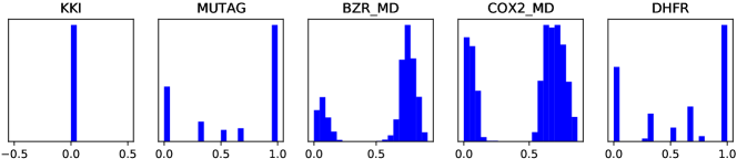
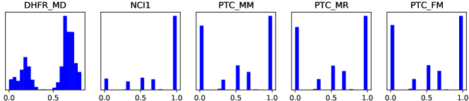
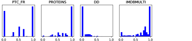
Figure 3: Illustration of the histogram of the homophily ratio $\alpha_{v}$ of nodes in each dataset. X-axis denotes the value of $\alpha_{v}$ and y-axis denotes the frequency (not shown here for clarity).

IV-C2 Ablation Study

In this section, we perform ablation study on each strategy used in IHGNN: 1) integration of the ego- and neighbor-embeddings of nodes, 2) separation of the ego- and neighbor-embeddings of nodes, 3) concatenation of the intermediate node embeddings from every layer, and 4) concatenation of all the node embeddings as the final graph-level readout function. The classification accuracy is reported in Table III. We observe that the IHGNN method outperforms both IHGNN-w/o-Inter. and IHGNN-w/o-Grap. on all the datasets. The former one does not concatenate the intermediate node embeddings from every layer and the latter one does not concatenate all the node embeddings as the final graph-level readout function (using instead the summation of all the node embeddings). On most of the datasets, IHGNN that adopts both the strategies of the integration and separation of the ego- and neighbor-embeddings of nodes performs better than that uses only one kind of strategy. On datasets NCI1 and PTC_MM, IHGNN-w/o-Integ. that does not use the integration of the ego- and neighbor-embeddings of nodes performs the best; on datasets COX2_MD and DHFR_MD, IHGNN-w/o-Sepa. that does not use the separation of the ego- and neighbor-embeddings of nodes performs the best. In conclusion, IHGNN which adopts all the four strategies achieves the best results on most of the datasets.

TABLE III: Comparison of classification accuracy (mean $\pm$ standard deviation) of IHGNN to its four variants on the benchmark datasets. IHGNN-w/o-Integ. stands for IHGNN without the integration of the ego- and neighbor-embeddings of nodes; IHGNN-w/o-Sepa. stands for IHGNN without the separation of the ego- and neighbor-embeddings of nodes; IHGNN-w/o-Inter. stands for IHGNN without the concatenation of the intermediate node embeddings from every layer (only using the node embeddings of the last layer); IHGNN-w/o-Grap. stands for IHGNN without the graph-level node embedding concatenation (using instead the summation of all the node embeddings as the graph-level readout function).

Dataset	IHGNN	IHGNN-w/o-Integ.	IHGNN-w/o-Sepa.	IHGNN-w/o-Inter.	IHGNN-w/o-Grap.
KKI	65.0$\pm$13.5	65.0$\pm$22.2	62.5$\pm$23.0	57.5$\pm$21.1	61.3$\pm$13.1
MUTAG	90.6$\pm$8.3	88.9$\pm$5.6	90.6$\pm$7.5	87.2$\pm$8.6	83.9$\pm$8.0
BZR_MD	75.7$\pm$6.2	72.7$\pm$7.6	74.3$\pm$8.2	71.7$\pm$7.6	72.0$\pm$9.8
COX2_MD	73.0$\pm$8.2	68.0$\pm$9.5	74.0$\pm$8.1	67.7$\pm$9.1	68.3$\pm$12.4
DHFR	85.5$\pm$2.6	84.0$\pm$5.2	80.7$\pm$4.1	83.9$\pm$3.2	82.7$\pm$3.6
DHFR_MD	74.6$\pm$8.8	72.1$\pm$9.9	76.2$\pm$5.6	70.5$\pm$7.8	70.3$\pm$8.3
NCI1	82.8$\pm$1.9	83.3$\pm$1.6	83.2$\pm$1.9	82.8$\pm$1.4	80.6$\pm$1.8
PTC_MM	69.7$\pm$6.6	70.3$\pm$6.9	67.3$\pm$7.5	68.2$\pm$7.8	70.0$\pm$6.7
PTC_MR	65.6$\pm$7.0	65.0$\pm$6.9	65.0$\pm$8.7	62.9$\pm$4.4	60.3$\pm$9.4
PTC_FM	65.3$\pm$11.1	62.6$\pm$5.9	63.2$\pm$7.4	63.8$\pm$7.6	59.7$\pm$8.2
PTC_FR	69.4$\pm$8.7	66.9$\pm$9.5	67.1$\pm$9.9	66.0$\pm$8.3	68.9$\pm$8.3
PROTEINS	77.1$\pm$5.1	75.8$\pm$3.8	75.2$\pm$5.6	76.5$\pm$5.0	65.1$\pm$5.0
DD	79.4$\pm$2.5	78.8$\pm$3.6	78.5$\pm$3.0	76.9$\pm$4.2	63.5$\pm$2.9
IMDB-MULTI	52.5$\pm$3.6	50.7$\pm$3.0	51.7$\pm$4.5	51.9$\pm$3.6	51.2$\pm$2.9

IV-C3 Parameter Sensitivity

In this section, we evaluate how the number of layers affect the performance of IHGNN, which is demonstrated in Figure 4. According to the node homophily ratio of each dataset illustrated in Figure 3, we select six representative datasets as follows: KKI, COX2_MD, PTC_FR, PROTEINS, DD, and IMDB-MULTI. We can see that the mean classification accuracy does not fluctuate much on all the datasets except COX2_MD, on which the mean classification accuracy increases with the increasing number of layers. A critical problem that GNNs face is the oversmoothing problem, i.e., the features of neighboring nodes tend to be indistinguishable when increasing the number of layers, which is caused by the graph Laplacian smoothing [34, 35, 36, 37]. However, this phenomenon is not obvious in our IHGNN, because we use the skip-connection strategy that concatenates all the intermediate node embeddings from every layer, which increases the expressive power.

(a) KKI

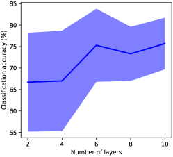
(b) COX2_MD

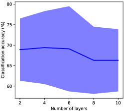
(c) PTC_FR

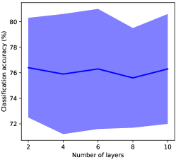
(d) PROTEINS

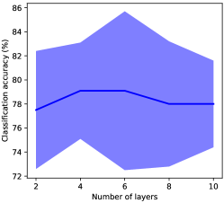
(e) DD

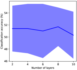
(f) IMDB-MULTI

Figure 4: Parameter sensitivity study for IHGNN. The solid line denotes the mean and the shaded area denotes the standard deviation. Because of using the skip-connection, IHGNN is not affected much by the oversmoothing problem, which is caused by the graph Laplacian smoothing when increasing the number of layers.

V Related Work

V-A Node Classification

Scarselli et al. [4] propose graph neural network (GNN) model to extend neural networks for processing graph data. The GNN model implements a function to map a graph into the Euclidean space. Shuman et al. [38] discuss several ways to define graph spectral domains for signal processing on graphs, and generalize fundamental operations such as filtering, translation, modulation, dilation, convolution, and downsampling to graph domains. The graph convolution operator is invented, which is the basis of graph convolutional neural networks. Since most of existing GNN models learn a message passing and aggregation function to embed nodes or graphs, Gilmer et al. [5] reformulate them into a single common framework called message passing neural networks (MPNNs).

ChebyNet [6] presents a formulation of CNNs in the context of spectral graph theory, which can be applied to design fast localized convolution filters on graphs. ChebyNet adopts Chebyshev polynomial to recursively compute the localized graph spectral filters with linear time complexity. GCN [7] proposes to use a localized first-order approximation of spectral graph convolutions for scalable learning on graphs. The localized first-order approximation leads to an elegant layer-wise propagation rule that allows for building deep models. JK-Nets [19] explores an architecture that selectively aggregates the output of each GCN layer. Since deep GCN is hard to train, JK-Nets does not perform much better. GG-NNs [39] is proposed for learning representations of the internal state during the process of producing a sequence of outputs from graphs. It incorporates GRU to the message passing and aggregation processes. LanczosNet [40] uses the Lanczos algorithm to efficiently construct low rank approximations of the graph Laplacian matrix for graph convolution. Through the Lanczos algorithm, it efficiently computes the power of the graph Laplacian matrix, exploits multi-scale information, and designs learnable spectral filters. PPNP [41] incorporates the personalized PageRank diffusion [42] into GNNs. The personalized PageRank diffusion propagates the learned node embeddings into their higher-order neighborhoods and aggregates all the information. In this way, it expands the number of layers in GNNs to infinity and improves node classification accuracy. GRAND [43] treats deep learning on graphs as a continuous diffusion process and GNNs as discretisations of an underlying partial differential equations (PDEs), which leads to a new class of GNNs that are able to mitigate the problems of depth, oversmoothing, bottlenecks, etc.

The above related works assume that the edges in a graph are homogeneous. However, in the real world, edges are formed by various reasons, and treating all edges homogeneously may deteriorate the classifier’s performance. To solve this problem, researchers have proposed to learn heterogeneous edge weights. GAT [44] computes the latent representations for each node in a graph by attending over its neighbors, following a self-attention strategy. It specifies different weights for different nodes in a neighborhood and thus achieves better performance than GNNs that do not use the attention mechanism. AGNN [45] develops a linear model that removes all the intermediate non-linear activation layers of GCN and learns edge weights with an attention mechanism. GraphSAGE [24] is developed for the inductive representation learning on graphs. It learns a function to generate embedding for each node by sampling and aggregating features from its local neighborhood. GraphSAGE with the max-pooling aggregator learns the edge weight between a node and its $K$-hop neighborhood.

In heterophilous graphs, connected nodes tend to have different class labels and dissimilar features. The message-passing based GNNs do not perform well in this scenario because of two factors: 1) they lose the structural information of nodes in neighborhoods as they only consider homophily, and 2) they lack the ability to capture long-range dependencies. To mitigate the limitations, Geom-GCN [46] proposes a new geometric aggregation scheme that includes three modules, i.e., node embedding, structural neighborhood, and bi-level aggregation. H₂GCN [23] identifies three designs to improve learning on heterophilous graphs. The three designs are ego- and neighbor-embedding separation, higher-order neighborhoods exploitation, and combination of intermediate representations. All the above GNNs are developed for node-level tasks such as node classification. By summing all the node embeddings, they can be extended to graph-level tasks such as graph classification. Recently, researchers have tried their endeavors to design GNNs especially for the task of graph classification.

V-B Graph Classification

DCNN [47] introduces a diffusion-convolution operation, which extends CNNs to graph-structured data. Diffusion-convolution operation generates a latent representation for a node or a graph by scanning a graph diffusion process across each node. However, it does not distinguish between the importance of different powers of the Laplacian matrix and introduces high-frequency noises into the learning process. DiffPool [25] is proposed to learn the hierarchical representations of graphs. It is a differentiable graph pooling module that learns a soft assignment of each node to a set of clusters at each layer. Each cluster corresponds to the coarsened input for the next layer. At each layer, DiffPool uses two separate GNNs to generate the embedding and assignment matrices without considering the relations between them. DGCNN [26] proposes to use the random walk probability transition matrix as graph Laplacian and relates itself to the Weisfeiler-Lehman subtree kernel [48, 2] and propagation kernel [49]. In addition, DGCNN develops a SortPooling layer to align nodes from different graphs, which is similar to our method.

Recently, researchers have developed various strategies to increase the expressive power of GNNs. GIN [11] studies the representational properties and limitations of GNNs. It proposes to use the MLP to learn the injective multiset functions for the neighbor aggregation and proves that its expressiveness is as powerful as the first order Weisfeiler-Lehman graph isomorphism test (1-WL) [12]. $k$-GNNs [13] investigates GNNs from a theoretical point of view and also relates it to the Weisfeiler-Lehman graph isomorphism test. To improve the expressiveness of GNNs, $k$-GNNs considers higher-order graph structures at multiple scales and performs message passing directly between graph substructures rather than individual nodes. The higher-order message passing strategy can capture some new structural information that cannot be captured by the node-level message passing strategy, which makes $k$-GNNs’ expressiveness as powerful as the 3-WL. PPGNs [14] explores and develops GNNs that have higher expressiveness while maintaining scalability, by applying the MLP to the feature dimension and matrix multiplication. Its expressiveness is also as powerful as the 3-WL. GNNML [16] is inpired by the recently proposed Matrix Language called MATLANG, which is developed by Brijder et al. [50, 51]. MATLANG has various operations on matrices such as summation, transposition, diagonalization, elementwise multiplication, and trace. This language relates these operations to the expressiveness of the 1-WL and the 3-WL. GNNML designs a new GNN architecture that contains as many of these matrix operations as possible to have an expressiveness as powerful as the 3-WL. However, all these high expressive models perform message passing between higher-order relations in graphs, which leads to computational overhead. Besides, they do not consider both the homophily and heterophily in graphs and thus their architectures are not adaptable to graphs with varying node homophily ratio. Our method IHGNN mitigates these problems. Nevertheless, IHGNN also has some limitations. For example, for the graph-level readout function, we concatenate all the node embeddings, which will increase the number of parameters to be learned compared with using the summation as the graph-level readout function.

Majority of the above literature designs GNNs in the spectral domain. There also exists some literature that designs GNNs in the spacial domain. ECC [52] learns filter weights conditioned on edge labels by a filter generation network, i.e., edges with the same labels have the same filter weights. Combined with the batch normalization and max pooling operations, it iteratively coarsens graphs. Finally, a global average pooling is adopted to generate the graph representation. PSCN [53] first orders nodes by the graph canonicalization tool Nauty [54], and then performs three operations, i.e., (1) node sequence selection, (2) neighborhood assembly, and (3) graph normalization, to generalize CNN to arbitrary graphs. DeepMap [55] solves the following two problems of graph kernels: (1) the elements in graph feature maps extracted by graph kernels are redundant, which leads to high-dimensional feature space, and (2) graph kernels cannot capture the higher-order complex interactions between nodes. DeepMap adopts breadth-first search and eigenvector centrality to generate an ordered and aligned node sequence for each graph and then applies CNN to generate deep representations for the graph feature maps.

Besides node classification and graph classification tasks, GNNs are being studied in the context of many different problems and applications such as anomaly detection [56, 57], event detection [58, 59], natural language processing [60, 61], and combinatorial problems of graphs [62, 63, 64]. It would be interesting to extend our study of the expressiveness of GNNs towards these objectives as well.

VI Conclusion

In this paper, we have developed a new GNN model called IHGNN for graphs with varying node homophily ratio, based on the two designs. Many existing GNNs fail to generalize to this setting and thus underperform on such graphs. Our designs distinguish not only between the integration and separation of the ego- and neighbor-embeddings of nodes in the $\mbox{COMBINE}(\cdot)$ operator used in GNNs, but also between each node embedding in the graph-level readout function. The two designs make IHGNN’s expressiveness as powerful as the 1-WL. Experiments show that IHGNN outperforms other state-of-the-art GNNs on graph classification. In the future, we would like to apply these two designs on GNNs that perform message passing between higher-order relations in graphs.

References

- [1] D. Haussler, “Convolution kernels on discrete structures,” Technical report, Department of Computer Science, University of California at Santa Cruz, Tech. Rep., 1999.
- [2] N. Shervashidze, P. Schweitzer, E. J. v. Leeuwen, K. Mehlhorn, and K. M. Borgwardt, “Weisfeiler-lehman graph kernels,” Journal of Machine Learning Research, vol. 12, no. Sep, pp. 2539–2561, 2011.
- [3] W. Ye, Z. Wang, R. Redberg, and A. Singh, “Tree++: Truncated tree based graph kernels,” IEEE Transactions on Knowledge and Data Engineering, 2019.
- [4] F. Scarselli, M. Gori, A. C. Tsoi, M. Hagenbuchner, and G. Monfardini, “The graph neural network model,” IEEE Transactions on Neural Networks, vol. 20, no. 1, pp. 61–80, 2008.
- [5] J. Gilmer, S. S. Schoenholz, P. F. Riley, O. Vinyals, and G. E. Dahl, “Neural message passing for quantum chemistry,” in Proceedings of the 34th International Conference on Machine Learning-Volume 70, 2017, pp. 1263–1272.
- [6] M. Defferrard, X. Bresson, and P. Vandergheynst, “Convolutional neural networks on graphs with fast localized spectral filtering,” in Advances in neural information processing systems, 2016, pp. 3844–3852.
- [7] T. N. Kipf and M. Welling, “Semi-supervised classification with graph convolutional networks,” International Conference on Learning Representations (ICLR), 2016.
- [8] N. Kriege and P. Mutzel, “Subgraph matching kernels for attributed graphs,” in Proceedings of the 29th International Coference on International Conference on Machine Learning, 2012, pp. 291–298.
- [9] A. K. Debnath, R. L. Lopez de Compadre, G. Debnath, A. J. Shusterman, and C. Hansch, “Structure-activity relationship of mutagenic aromatic and heteroaromatic nitro compounds. correlation with molecular orbital energies and hydrophobicity,” Journal of medicinal chemistry, vol. 34, no. 2, pp. 786–797, 1991.
- [10] V. P. Dwivedi, C. K. Joshi, T. Laurent, Y. Bengio, and X. Bresson, “Benchmarking graph neural networks,” arXiv preprint arXiv:2003.00982, 2020.
- [11] K. Xu, W. Hu, J. Leskovec, and S. Jegelka, “How powerful are graph neural networks?” International Conference on Learning Representations (ICLR), 2018.
- [12] A. Leman and B. Weisfeiler, “A reduction of a graph to a canonical form and an algebra arising during this reduction,” Nauchno-Technicheskaya Informatsiya, vol. 2, no. 9, pp. 12–16, 1968.
- [13] C. Morris, M. Ritzert, M. Fey, W. L. Hamilton, J. E. Lenssen, G. Rattan, and M. Grohe, “Weisfeiler and leman go neural: Higher-order graph neural networks,” in Proceedings of the AAAI Conference on Artificial Intelligence, vol. 33, no. 01, 2019, pp. 4602–4609.
- [14] H. Maron, H. Ben-Hamu, H. Serviansky, and Y. Lipman, “Provably powerful graph networks,” Advances in Neural Information Processing Systems, 2019.
- [15] H. Maron, H. Ben-Hamu, N. Shamir, and Y. Lipman, “Invariant and equivariant graph networks,” arXiv preprint arXiv:1812.09902, 2018.
- [16] M. Balcilar, P. Héroux, B. Gaüzère, P. Vasseur, S. Adam, and P. Honeine, “Breaking the limits of message passing graph neural networks,” International Conference on Machine Learning (ICML), 2021.
- [17] P. W. Battaglia, J. B. Hamrick, V. Bapst, A. Sanchez-Gonzalez, V. Zambaldi, M. Malinowski, A. Tacchetti, D. Raposo, A. Santoro, R. Faulkner et al., “Relational inductive biases, deep learning, and graph networks,” arXiv preprint arXiv:1806.01261, 2018.
- [18] M. Zaheer, S. Kottur, S. Ravanbakhsh, B. Poczos, R. R. Salakhutdinov, and A. J. Smola, “Deep sets,” Advances in Neural Information Processing Systems, vol. 30, 2017.
- [19] K. Xu, C. Li, Y. Tian, T. Sonobe, K.-i. Kawarabayashi, and S. Jegelka, “Representation learning on graphs with jumping knowledge networks,” in International Conference on Machine Learning (ICML), 2018, pp. 5449–5458.
- [20] F. Harary, “Graph theory addison-wesley reading ma usa,” 1969.
- [21] K. Hornik, M. Stinchcombe, and H. White, “Multilayer feedforward networks are universal approximators,” Neural networks, vol. 2, no. 5, pp. 359–366, 1989.
- [22] K. Hornik, “Approximation capabilities of multilayer feedforward networks,” Neural networks, vol. 4, no. 2, pp. 251–257, 1991.
- [23] J. Zhu, Y. Yan, L. Zhao, M. Heimann, L. Akoglu, and D. Koutra, “Beyond homophily in graph neural networks: Current limitations and effective designs,” Advances in Neural Information Processing Systems, 2020.
- [24] W. Hamilton, Z. Ying, and J. Leskovec, “Inductive representation learning on large graphs,” in Advances in Neural Information Processing Systems, 2017, pp. 1024–1034.
- [25] R. Ying, J. You, C. Morris, X. Ren, W. L. Hamilton, and J. Leskovec, “Hierarchical graph representation learning with differentiable pooling,” Advances in Neural Information Processing Systems, 2018.
- [26] M. Zhang, Z. Cui, M. Neumann, and Y. Chen, “An end-to-end deep learning architecture for graph classification,” in Thirty-Second AAAI Conference on Artificial Intelligence, 2018.
- [27] D. P. Kingma and J. Ba, “Adam: A method for stochastic optimization,” International Conference on Learning Representations (ICLR), 2014.
- [28] S. Pan, J. Wu, X. Zhu, G. Long, and C. Zhang, “Task sensitive feature exploration and learning for multitask graph classification,” IEEE transactions on cybernetics, vol. 47, no. 3, pp. 744–758, 2017.
- [29] J. J. Sutherland, L. A. O’brien, and D. F. Weaver, “Spline-fitting with a genetic algorithm: A method for developing classification structure- activity relationships,” Journal of chemical information and computer sciences, vol. 43, no. 6, pp. 1906–1915, 2003.
- [30] N. Wale, I. A. Watson, and G. Karypis, “Comparison of descriptor spaces for chemical compound retrieval and classification,” Knowledge and Information Systems, vol. 14, no. 3, pp. 347–375, 2008.
- [31] K. M. Borgwardt, C. S. Ong, S. Schönauer, S. Vishwanathan, A. J. Smola, and H.-P. Kriegel, “Protein function prediction via graph kernels,” Bioinformatics, vol. 21, no. suppl_1, pp. i47–i56, 2005.
- [32] P. D. Dobson and A. J. Doig, “Distinguishing enzyme structures from non-enzymes without alignments,” Journal of molecular biology, vol. 330, no. 4, pp. 771–783, 2003.
- [33] P. Yanardag and S. Vishwanathan, “Deep graph kernels,” in Proceedings of the 21th ACM SIGKDD International Conference on Knowledge Discovery and Data Mining. ACM, 2015, pp. 1365–1374.
- [34] Q. Li, Z. Han, and X.-M. Wu, “Deeper insights into graph convolutional networks for semi-supervised learning,” in Thirty-Second AAAI Conference on Artificial Intelligence, 2018.
- [35] F. Wu, T. Zhang, A. Holanda de Souza, C. Fifty, T. Yu, and K. Q. Weinberger, “Simplifying graph convolutional networks,” Proceedings of Machine Learning Research, 2019.
- [36] H. NT and T. Maehara, “Revisiting graph neural networks: All we have is low-pass filters,” arXiv preprint arXiv:1905.09550, 2019.
- [37] W. Ye, Z. Huang, Y. Hong, and A. Singh, “Graph neural diffusion networks for semi-supervised learning,” arXiv preprint arXiv:2201.09698, 2022.
- [38] D. I. Shuman, S. K. Narang, P. Frossard, A. Ortega, and P. Vandergheynst, “The emerging field of signal processing on graphs: Extending high-dimensional data analysis to networks and other irregular domains,” IEEE signal processing magazine, vol. 30, no. 3, pp. 83–98, 2013.
- [39] Y. Li, D. Tarlow, M. Brockschmidt, and R. Zemel, “Gated graph sequence neural networks,” 2016.
- [40] R. Liao, Z. Zhao, R. Urtasun, and R. S. Zemel, “Lanczosnet: Multi-scale deep graph convolutional networks,” International Conference on Learning Representations (ICLR), 2019.
- [41] J. Klicpera, A. Bojchevski, and S. Günnemann, “Predict then propagate: Graph neural networks meet personalized pagerank,” in International Conference on Learning Representations (ICLR), 2019.
- [42] R. Andersen, F. Chung, and K. Lang, “Local graph partitioning using pagerank vectors,” in 2006 47th Annual IEEE Symposium on Foundations of Computer Science (FOCS’06). IEEE, 2006, pp. 475–486.
- [43] B. P. Chamberlain, J. Rowbottom, M. Gorinova, S. Webb, E. Rossi, and M. M. Bronstein, “Grand: Graph neural diffusion,” International Conference on Machine Learning (ICML), 2021.
- [44] P. Veličković, G. Cucurull, A. Casanova, A. Romero, P. Lio, and Y. Bengio, “Graph attention networks,” International Conference on Learning Representations (ICLR), 2017.
- [45] K. K. Thekumparampil, C. Wang, S. Oh, and L.-J. Li, “Attention-based graph neural network for semi-supervised learning,” arXiv preprint arXiv:1803.03735, 2018.
- [46] H. Pei, B. Wei, K. C.-C. Chang, Y. Lei, and B. Yang, “Geom-gcn: Geometric graph convolutional networks,” International Conference on Learning Representations (ICLR), 2020.
- [47] J. Atwood and D. Towsley, “Diffusion-convolutional neural networks,” in Advances in neural information processing systems, 2016, pp. 1993–2001.
- [48] N. Shervashidze and K. M. Borgwardt, “Fast subtree kernels on graphs,” in Advances in neural information processing systems, 2009, pp. 1660–1668.
- [49] M. Neumann, R. Garnett, C. Bauckhage, and K. Kersting, “Propagation kernels: efficient graph kernels from propagated information,” Machine Learning, vol. 102, no. 2, pp. 209–245, 2016.
- [50] R. Brijder, F. Geerts, J. V. D. Bussche, and T. Weerwag, “On the expressive power of query languages for matrices,” ACM Transactions on Database Systems (TODS), vol. 44, no. 4, pp. 1–31, 2019.
- [51] F. Geerts, “On the expressive power of linear algebra on graphs,” Theory of Computing Systems, vol. 65, no. 1, pp. 179–239, 2021.
- [52] M. Simonovsky and N. Komodakis, “Dynamic edge-conditioned filters in convolutional neural networks on graphs,” in Proceedings of the IEEE conference on computer vision and pattern recognition, 2017, pp. 3693–3702.
- [53] M. Niepert, M. Ahmed, and K. Kutzkov, “Learning convolutional neural networks for graphs,” in International conference on machine learning (ICML), 2016, pp. 2014–2023.
- [54] B. D. McKay and A. Piperno, “Practical graph isomorphism, ii,” Journal of Symbolic Computation, vol. 60, pp. 94–112, 2014.
- [55] W. Ye, O. Askarisichani, A. Jones, and A. Singh, “Learning deep graph representations via convolutional neural networks,” IEEE Transactions on Knowledge and Data Engineering, 2020.
- [56] A. Protogerou, S. Papadopoulos, A. Drosou, D. Tzovaras, and I. Refanidis, “A graph neural network method for distributed anomaly detection in iot,” Evolving Systems, vol. 12, no. 1, pp. 19–36, 2021.
- [57] Y. Wang, J. Zhang, S. Guo, H. Yin, C. Li, and H. Chen, “Decoupling representation learning and classification for gnn-based anomaly detection,” in Proceedings of the 44th International ACM SIGIR Conference on Research and Development in Information Retrieval, 2021, pp. 1239–1248.
- [58] M. Kosan, A. Silva, S. Medya, B. Uzzi, and A. Singh, “Event detection on dynamic graphs,” arXiv preprint arXiv:2110.12148, 2021.
- [59] S. Deng, H. Rangwala, and Y. Ning, “Learning dynamic context graphs for predicting social events,” in Proceedings of the 25th ACM SIGKDD International Conference on Knowledge Discovery & Data Mining, 2019, pp. 1007–1016.
- [60] Y. Zhang, X. Yu, Z. Cui, S. Wu, Z. Wen, and L. Wang, “Every document owns its structure: Inductive text classification via graph neural networks,” arXiv preprint arXiv:2004.13826, 2020.
- [61] S. Medya, M. Rasoolinejad, Y. Yang, and B. Uzzi, “An exploratory study of stock price movements from earnings calls,” The Web Conference, 2022.
- [62] E. Khalil, H. Dai, Y. Zhang, B. Dilkina, and L. Song, “Learning combinatorial optimization algorithms over graphs,” Advances in neural information processing systems, vol. 30, 2017.
- [63] S. Manchanda, A. Mittal, A. Dhawan, S. Medya, S. Ranu, and A. Singh, “Gcomb: Learning budget-constrained combinatorial algorithms over billion-sized graphs,” Advances in Neural Information Processing Systems, vol. 33, pp. 20 000–20 011, 2020.
- [64] R. Ranjan, S. Grover, S. Medya, V. Chakaravarthy, Y. Sabharwal, and S. Ranu, “A neural framework for learning subgraph and graph similarity measures,” arXiv preprint arXiv:2112.13143, 2021.