Distributed-Memory Sparse Kernels for Machine Learning

Abstract

Sampled Dense Times Dense Matrix Multiplication (SDDMM) and Sparse Times Dense Matrix Multiplication (SpMM) appear in diverse settings, such as collaborative filtering, document clustering, and graph embedding. Frequently, the SDDMM output becomes the input sparse matrix for a subsequent SpMM operation. Existing work has focused on shared memory parallelization of these primitives. While there has been extensive analysis of communication-minimizing distributed 1.5D algorithms for SpMM, no such analysis exists for SDDMM or the back-to-back sequence of SDDMM and SpMM, termed FusedMM. We show that distributed memory 1.5D and 2.5D algorithms for SpMM can be converted to algorithms for SDDMM with identical communication costs and input / output data layouts. Further, we give two communication-eliding strategies to reduce costs further for FusedMM kernels: either reusing the replication of an input dense matrix for the SDDMM and SpMM in sequence, or fusing the local SDDMM and SpMM kernels.

We benchmark FusedMM algorithms on Cori, a Cray XC40 at LBNL, using Erdős-Rényi random matrices and large real-world sparse matrices. On 256 nodes with 68 cores each, 1.5D FusedMM algorithms using either communication eliding approach can save at least 30% of time spent exclusively in communication compared to executing a distributed-memory SpMM and SDDMM kernel in sequence. Our 2.5D communication-eliding algorithms save 21% of communication time compared to the unoptimized sequence. On real-world matrices with hundreds of millions of edges, all of our algorithms exhibit at least a 10x speedup over the SpMM algorithm in PETSc. On these matrices, our communication-eliding techniques exhibit runtimes up to 1.6 times faster than an unoptimized sequence of SDDMM and SpMM. We embed and test the scaling of our algorithms in real-world applications, including collaborative filtering via alternating-least-squares and inference for attention-based graph neural networks.

I Introduction

Sampled Dense-Dense Matrix Multiplication (SDDMM) and Sparse-Times-Dense Matrix Multiplication (SpMM) have become workhorse kernels in a variety of computations. Their use in matrix completion [1] and document similarity computation [2] is well documented, and they are the main primitives used in graph learning [3]. The recent interest in Graph Neural Networks (GNNs) with self-attention has led libraries such as Amazon Deep Graph Library (DGL) [4] to expose SDDMM and SpMM primitives to users. Typical applications make a call to an SDDMM operation and feed the sparse output to an SpMM operation, repeating the pair several times with the same nonzero pattern (but possibly different values) for the sparse matrix. We refer to the back-to-back sequence of an SDDMM and SpMM as FusedMM.

Several works optimize SDDMM and SpMM kernels in shared memory environments, or on accelerators such as GPUs [5, 6, 7]. Separately, there have been prior efforts  [8, 9, 10] to optimize distributed memory SpMM by minimizing processor to processor communication. There is no significant work, however, on distributed algorithms for SDDMM or FusedMM.

We make three main contributions. First, we show that every sparsity-agnostic distributed-memory algorithm for SpMM can be converted into a distributed memory algorithm for SDDMM that uses the same input / output data distribution and has identical communication cost. Second, we give two methods to elide communication when executing an SDDMM and SpMM in sequence (FusedMM): replication reuse, which elides a second replication of an input matrix, and local kernel fusion, which allows local SDDMM and SpMM operations to execute on the same processor without intervening communication. These methods not only eliminate unnecessary communication rounds, they also enable algorithms that replicate dense matrices to scale to higher or lower replication factors (depending on which of the two methods used). Third, we demonstrate, both in theory and practice, these algorithms that replicate or shift sparse matrices perform best when the ratio of nonzeros in the sparse matrix to the number of nonzeros in the dense matrices is sufficiently low. When the number of nonzeros in the sparse matrix approaches the number of nonzeros in either of the dense matrices, algorithms that shift or replicate dense matrices become favorable. Our work gives, to the best of our knowledge, the first benchmark of 1.5D SpMM and SDDMM algorithms that cyclically shift sparse matrices and replicate a dense matrix, which enables efficient communication scaling when the input dense matrices are tall and skinny. It also gives the first head-to-head comparison between sparse shifting and dense shifting 1.5D algorithms, which we show outperform each other depending on the problem setting.

II Definitions

Symbol	Description
$S,R$	$m\times n$ sparse matrix
$A$	$m\times r$ dense matrix
$B$	$n\times r$ dense matrix
$\phi$	The ratio $\textrm{nnz(S)}/nr$
$p$	Total processor count
$c$	Replication Factor

TABLE I: Symbol Definitions

Let $A\in\mathbb{R}^{m\times r},B\in\mathbb{R}^{n\times r}$ be dense matrices and let $S\in\mathbb{R}^{m\times n}$ be a sparse matrix. The SDDMM operation produces a sparse matrix with sparsity structure identical to $S$ given by

$$\textrm{SDDMM}(A,B,S):=S*(A\cdot B^{T})$$ (1)

where $*$ denotes elementwise multiplication and $\cdot$ denotes matrix-matrix multiplication. Computing the output with a dense matrix multiplication followed by element-wise multiplication with $S$ is inefficient, since we only need to compute the output entries at the nonzero locations of $S$.

For clarity of notation when describing our distributed memory algorithms, we distinguish between the SpMM operation involving $S$ that takes $B$ as an input vs. the operation involving $S^{T}$ that takes $A$ as an input. Specifically, define

SpMMA(S, B) $$:=S\cdot B$$

SpMMB(S, A) $$:=S^{T}\cdot A$$

where the suffix A or B on each operation refers to the matrix with the same shape as the output. The distinction is useful for applications such as alternating least squares and graph attention networks, which require both operations at different points in time. Finally, we borrow notation from prior works on the SDDMM-SpMM sequence [11] and use FusedMMA, FusedMMB to denote operations that are compositions of SDDMM with SpMMA or SpMMB, given as

$$\textrm{FusedMMA}(S,A,B) :=\textrm{SpMMA}(\textrm{SDDMM}(A,B,S),B)$$

$$\textrm{FusedMMB}(S,A,B) :=\textrm{SpMMB}(\textrm{SDDMM}(A,B,S),A)$$

III Existing Work

III-A Shared Memory Optimization

Local SpMM and SDDMM operations are bound by memory bandwidth compared to dense matrix multiplication. Accelerating either SpMM or SDDMM in a shared memory environment, such as a single CPU node or GPU, typically involves blocking a loop over the nonzeros of $S$ to optimize cache reuse of the dense matrices [6]. For blocked SDDMM and SpMM kernels, the traffic between fast and slow memory is exactly modeled by the edgecut-1 metric of a hypergraph partition induced on $S$ (treating the rows of $S$ as hyperedges and the columns as vertices, with nonzeros indicating pins). Jiang et al. [7] reorder the sparse matrix to minimize the connectivity metric, thereby reducing memory traffic. Instead of reordering $S$, Hong et al. [5] adaptively choose a blocking shape tuned to the sparsity structure to optimize performance. Both optimizations require expensive processing steps on the sparse matrix $S$, which are typically amortized away by repeated calls to the kernel.

III-B Distributed Sparsity-Aware Algorithms

We can divide distributed-memory implementations for both SpMM and SDDMM into two categories: sparsity-aware algorithms, and sparsity-agnostic bulk communication approaches. In the former category, the dense input matrices are partitioned among processors along with the sparse matrix nonzeros $(i,j)$, such that each processor owns at least one of $A_{i:}$ or $B_{j:}$. When processing $(i,j)$, if a processor does not own one of the two dense rows needed, it fetches the embedding from another processor that owns it [10]. Such approaches work well when $S$ is very sparse. They also benefit from graph / hypergraph partitioning to reorder the sparse matrix, which can reduce the number of remote fetches that each processor must make while maintaining load balance. Such approaches suffer, however, from the overhead of communicating the specific embeddings requested by processors, which typically requires round-trip communication. As $S$ gets denser, processors are better off broadcasting all of their embeddings.

III-C Sparsity Agnostic Bulk Communication Algorithms

Sparsity agnostic algorithms resemble distributed dense matrix multiplication algorithms by broadcasting, shifting, and reducing block rows and block columns of $A,B$, and $S$. These methods cannot significantly benefit from graph partitioning and they often rely on a random permutation of the sparse matrix to load balance among processors.

Such algorithms are typically described as 1D, 1.5D, 2D, 2.5D, or 3D. 1D and 2D algorithms are memory-optimal, with processors requiring no more aggregate memory than the storage required for inputs and outputs (up to a small constant factor for communication buffering). 1.5D, 2.5D, and 3D algorithms increase collective memory consumption of at least one of the three operands to asymptotically decrease communication costs. In this work, we will consider only 1.5D and 2.5D algorithms, since 1D, 2D, and 3D algorithms are special cases of these two.

Koanantakool et al. show when $A,B$ and $S$ are all square, 1.5D SpMM algorithms that cyclically shift the sparse matrix yield superior performance [8]. They only benchmark multiplication of all square matrices, which does not cover the more common case where $r\ll m,n$. For graph embedding problems, $r$ is typically between $64$ and $512$, whereas $m$ and $n$ can be in tens to hundreds of milllions. For this case of tall-skinny dense matrices, Tripathy et al. introduced CAGNET, which trains graph neural networks on hundreds of GPUs using 1.5D and 2.5D distributed SpMM operations [12]. They, along with Selvitopi et al. [9], showed that 2D algorithms for SpMM suffer from diminished arithmetic intensity as processor count increases. In contrast, both demonstrate that 1.5D algorithms communicating dense matrices exhibit excellent scaling with processor count. Selvitopi et al. did not consider 2.5D algorithms, however, and neither work benchmarked 1.5D algorithms that cyclically shift sparse matrices. In addition, the 2.5D algorithms in CAGNET only replicate the dense matrix, whereas it is also possible to construct implementations that only replicate the sparse matrix.

III-D Background on Dense Distributed Linear Algebra

Our sparsity-agnostic algorithms resemble 1.5D and 2.5D variants of the the Cannon and SUMMA distributed dense GEMM algorithms [13], [14]. In the 2.5D Cannon-like algorithm to compute compute the matrix product $X=YZ$, the submatrix domains of the output $X$ are replicated among processors [15]. E.g., for every entry $X_{ij}$, different processors compute different parts of the inner product $Y_{i:}\cdot Y_{:j}$ and reduce their results at the end. The inputs are both propagated during the algorithm: submatrices of $A$ and $B$ are cyclically shifted between processors in stages. The SUMMA algorithm replaces the stages of cyclic shifts with broadcast collectives. 1.5D variants of these algorithms keep at least one of the three matrices stationary: submatrices of a stationary matrix are distributed among processors, but they are not broadcast, reduced, or shifted. It is possible to modify these algorithms so that an input matrix is replicated rather than an output.

Our algorithm design is dictated by choosing which submatrices we keep stationary, replicate, and propagate. While these choices do not matter for dense GEMM if all matrices are square, they impact our kernels due to the sparsity of $S$ and the extremely rectangular shapes of $A$ and $B$.

Kwasniewski et al. recently proposed COSMA [16], which uses the classic red-blue pebbling game to design an optimal parallelization scheme for distributed dense GEMM with matrices of varying shapes. Their communication-minimizing algorithms achieve excellent performance relative to SCALAPACK and recent high performance matrix multiplication work. COSMA, however, does not account for sparsity in either inputs or outputs. Our work, furthermore, focuses on the FusedMM computation pattern commonly found in applications, which provides further opportunities for communication minimization than considering the SpMM and SDDMM kernels in isolation.

IV Distributed Memory Algorithms for SDDMM and FusedMM

This section highlights the connection between SpMM and SDDMM and gives a high-level procedure to convert between algorithms that compute each one. This enables us to use a single input distribution to compute SDDMM, SpMMA, and SpMMB, at the cost of possibly replicating the sparse matrix $S$ by a factor of 2 to store its transpose. Each kernel requires the same amount of communication. Next, we give two communication elision strategies when we execute an SDDMM and an SpMM operation in sequence, with the output of the SDDMM feeding into the SpMM (a FusedMM operation). Optimizing for the sequence of the two kernels reduces communication overhead compared to simply executing one distributed algorithm followed by the other. Subsequently, we detail the implementation of those high-level strategies.

IV-A The Connection between SDDMM and SpMM

SDDMM and SpMM have identical data access patterns, which becomes clear when we compare their serial algorithms (take SpMMA here). Letting sparse matrix $R$ be the SDDMM output and letting $(i,j)$ index a nonzero entry of $S$, we have $R_{ij}=S_{ij}\left(A_{i:}\cdot B_{j,:}^{T}\right)$ with $R$ set to zero where $S$ is 0. Compare this equation to each step required to compute $A\mathrel{{+}{=}}\textrm{SpMMA}(S,B)$: for every nonzero $(i,j)$ of $S$, we perform the update $A_{i:}\mathrel{{+}{=}}S_{ij}B_{j:}$. For both SDDMM and SpMMA, each nonzero of $S$ results in an interaction between a row of $A$ and a row of $B$.

Now consider any distributed memory algorithm for SpMMA that does not replicate its input or output matrices during computation. For each nonzero $(i,j)$ and for every index $k\in\left[1,r\right]$, this algorithm must co-locate $S_{ij}$, $A_{ik}$, and $B_{jk}$ on some processor and compute $A_{ik}\mathrel{{+}{=}}S_{ij}B_{jk}$. Transform the algorithm as follows:

1. Change the input sparse matrix $S$ to an output matrix initialized to 0.

2. Change $A$ from an output matrix to an input matrix.

3. Have each processor execute local update $S_{ij}\mathrel{{+}{=}}A_{ik}B_{jk}$.

Then for all nonzeros $(i,j)$ and every index $k\in\left[1,r\right]$, the processors collectively execute computations to overwrite $S$ with $AB^{T}$ masked at the nonzeros of $S$. This is exactly the SDDMM operation up to multiplication of $AB^{T}$ with the values initially in $S$. If the output distribution of $S$ is identical to its input distribution after execution, then the post-multiplication with the initial values in $S$ does not require additional communication. A similar transformation converts an algorithm for SpMMB into an algorithm for SDDMM.

We can extend this transformation procedure to algorithms that replicate input and output matrices. Typically, inputs are replicated via broadcast, while output replication requires a reduction at the end of the algorithm to sum up temporary buffers across processors. Since we interchange in the input / output role between matrices $A$ and $S$, we convert broadcasts of the values of $S$ in SpMMA to reductions of its values in SDDMM, and reductions of $A$ to broadcasts.

Algorithms 1 and 2 illustrate the transformation procedure outlined above by giving unified algorithms to compute SDDMM, SpMMA, and SpMMB. The local update executed by each processor changes based on the kernel being executed, and initial broadcasts / terminal reductions depend on whether matrices function as inputs or outputs.

IV-B Strategies for Distributed Memory FusedMM

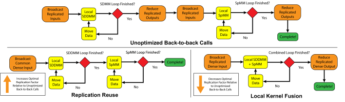
Figure 1: Communication eliding strategies illustrated. Crucially, the benefit from replication reuse and local kernel fusion arises from an increased or decreased optimal replication factor, not just the elimination of communication phases.

FusedMMA computes each row of its output as

$$\textrm{FusedMMA}(A,B,S)_{i:}:=\sum_{j\ |\ (i,j)\in nnz(S)}S_{ij}\langle A_{i:},B_{j:}\rangle B_{j:}$$

which is a sum of rows $j$ of matrix $B$ weighted by the dot products between rows $j$ of $B$ and rows $i$ of $A$. The analogous equation for FusedMMA replaces $S_{ij}$ with $S^{T}_{ij}=S_{ji}$. The simplest distributed implementation for FusedMMA computes the intermediate SDDMM, stores it temporarily, and feeds the result directly to SpMMA, exploiting the common data layout for inputs and outputs explainting in the previous section. The communication cost for this implementation is twice that of either a single SpMMA operation or SDDMM operation. Such an algorithm for FusedMMA takes the following structure:

1. Replicate dense matrices $A,B$ in preparation for SDDMM (if either $A$ or $B$ is replicated)

2. Propagate matrices, compute SDDMM

3. Reduce SDDMM output $R$ (if sparse matrix is replicated)

4. Replicate dense matrix $B$ in preparation for SpMMA (if $B$ is replicated)

5. Propagate matrices, compute SpMMA

6. Reduce output matrix $A$ (if $A$ is replicated)

In the outline above, propagation refers to any communication that excludes replication of inputs / outputs (for example, cyclic shifts of buffers in Cannon’s algorithm). Increased replication factors allow us to decrease propagation cost, but increase the required memory and result in a higher cost to perform the replication. Choosing the optimal replication factor involves minimizing the sum of the communication overhead paid in replication and propagation. We can save communication in two ways: first by reducing the replication cost, and second by reducing the propagation cost. Figure 1 illustrates both.

(1) Replication Reuse: This approach performs only a single replication of an input matrix in both the SDDMM and SpMM computations. If we replicate the dense matrix $B$, before the SDDMM operation, we don’t require a second replication before the SpMM phase, nor do we need a reduction of the output buffer.

(2) Local Kernel Fusion: This approach combines the two propagation steps, 2 and 5, into a single phase while only replicating matrix $A$. Using locally available data at each propagation step, it requires performing a local SDDMM and SpMM in sequence without intermediate communication. Thus, local kernel fusion with any data distribution that divides $A$ and $B$ by columns would yield an incorrect result. From the standard definition of FusedMMA, we must compute the dot product $\langle A_{i:},B_{j:}\rangle$ that scales every row of $B$ before aggregating those rows, requiring us to complete the SDDMM before performing any aggregation. The 1.5D algorithm that replicates and shifts dense matrices (Section V) co-locates entire rows of $A$ and $B$ on the same processor during the stages of computation, and is the only candidate that can take advantage of local kernel fusion. Besides the communication savings that they offer, optimized local FusedMM functions (e.g., [11]) can improve performance by eliding intermediate storage of the SDDMM result.

Although applying either method would provide moderate communication savings without modifying any other aspect of the algorithm, their utility really lies in allowing us to change the degree of replication for any algorithm that replicates a dense matrix. Algorithms that employ replication reuse can achieve lower communication overhead at higher replication factors compared to an unoptimized sequence of calls. Intuitively, increasing the replication factor enables the algorithm to trade away more overhead in the propagation phase before the cost of replication becomes overwhelming. By contrast, algorithms that employ local kernel fusion can achieve lower communication overhead at lower replication factors. The algorithm requires less replication to balance off the lower cost of propagation. Note that these strategies are mutually exclusive; applying them both to 1.5D dense shifting algorithms would require propagating a separate accumulation buffer in the propagation phase, which destroys the benefit of local kernel fusion.

While we have discussed strategies for FusedMMA, we obtain algorithms for FusedMMB by interchanging the roles of $A$ and $B$ and replacing matrix $S$ with its transpose $S^{T}$. In practice, this amounts to storing two copies of the sparse matrix across all processors, one with the coordinates transposed.

V Algorithm Descriptions

We consider formulations for SpMM detailed previously [8, 12, 9], but some with key modifications. We arrive at each algorithm by deciding which of the three matrices $A,B$, and $S$ to replicate, propagate, or keep stationary (see figure 2). We consider formulations where only a single matrix is replicated enabling us to scale to higher replication factors and take advantage of both communication-eliding strategies described above.

Figure 2: Design Choices in SpMM Algorithms. We do not consider the 1.5D sparse replicating, dense shifting algorithm, since it is inferior to the 2.5D sparse replicating algorithm.

Let $p$ be the total processor count. We list the input distributions of all matrices in Table II. Each matrix is partitioned by blocks into a grid with the specified dimension. The product of these dimensions may exceed the total processor count because processors can own multiple non-contiguous blocks, as in block row / column cyclic distributions. The third column of Table II gives the processor that initially owns a block $(i,j)$ as an $(u,v)$ or $(u,v,w)$ tuple, which identifies the processor position within a 2D / 3D grid. For the 2.5D sparse replicating algorithm, “*” means all processors along the third axis of the grid share the coordinates of block $(i,j)$. Figure 3 illustrates the data movement in our algorithms for 8 processors with a replication factor of 2. We will refer to the grid axis along which inputs are reduced or gathered as the “fiber axis”. It is the second dimension of the computational grid for 1.5D algorithms and the third dimension for 2.5D algorithms.

To analyze our algorithms, we use the $\alpha{\text{-}}\beta\text{-}\gamma$ model where $\alpha$ is the per-message latency, $\beta$ is the inverse-bandwidth, and $\gamma$ is the cost per FLOP performed locally on each processor. Since our algorithms communicate blocks of matrices, they exchange at most a small multiple of $p$ messages, each of which is a large block of a matrix. Therefore, we focus on minimizing the number of data words communicated by each processor, the coefficient of inverse-bandwidth in our model. In the analysis that follows, we use “communication cost” to mean the maximum amount of time that any processor spends sending and receiving messages.

We assume sends and receives can make independent progress on each node and use the costs for collectives in the literature [17]. To aid the analysis, assume $m\approx n$, and let $\phi$ be the ratio of the number of nonzeros in $S$ to the number of nonzeros of dense matrix $B$, i.e. $\phi=\textrm{nnz}(S)/nr$.

Matrix	Grid	Owner of Block $(i,j)$
1.5D Dense Shifting
A	$p\times 1$	$(i/c,i\%c)$
B	$p\times 1$	$(i/c,i\%c)$
S,R	$(p/c)\times p$	$(i,j\%c)$
1.5D Sparse Shifting
A	$p\times(p/c)$	$(j,i\%c)$
B	$p\times(p/c)$	$(j,i\%c)$
S,R	$1\times p$	$(j/c,j\%c)$
2.5D Dense Replicating
A	$\sqrt{pc}\times\sqrt{p/c}$	$(i/c,j,i\%c)$
B	$\sqrt{pc}\times\sqrt{p/c}$	$(i/c,j,i\%c)$
S,R	$\sqrt{p/c}\times\sqrt{pc}$	$(i,j/c,j\%c)$
2.5D Sparse Replicating
A	$p\times\sqrt{p/c}$	$(i/c,j,i\%c)$
B	$\sqrt{p/c}\times p$	$(i,j/c,j\%c)$
S,R	$\sqrt{p/c}\times\sqrt{p/c}$	$(i,j,*)$

TABLE II: Input Matrix Distributions Before Replication

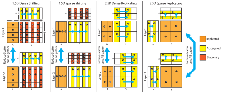
Figure 3: Data movement after replication, illustrated for $p=8$ processors and replication factor $c=2$. Within each layer, submatrices shown in yellow are cyclically shifted from processor to processor (propagation) in the direction indicated by single-headed blue arrows. Submatrices in orange are replicated across layers and participate in reduce-scatter / all-gather operations outside the propagation phase. Submatrices in red remain stationary on each processor. Black numbered circles give the processor owning each submatrix at the beginning of each algorithm (note the initial skew for 2.5D algorithms).

V-A 1.5D Dense Shifting, Dense Replicating

1.5D algorithms operate on a $(p/c)\times c$ processor grid, where $c\geq 1$ is the replication factor. We can interpret the 1.5D dense shifting, dense replicating algorithm as $c$ layers of concurrently executing 1D algorithms. To decrease communication as the processor count increases, the 1.5D dense shifting, dense replicating algorithm replicates one of the two dense matrix inputs, propagates the other dense matrix, and keeps the remaining sparse matrix stationary on each processor.

The procedure is detailed in Algorithm 1 and illustrated in Figure 3. The sparse matrix $S$ is stored with a column block cyclic distribution across the grid layers. The processors begin by allocating a buffer $T$ for the replicated matrix $A$, keeping $T$ initially 0 if $A$ is an output buffer and otherwise all-gathering blocks of $A$ of size $(n/p)\times r$ within each fiber axis if $A$ is an input (replication). For $p/c$ phases, algorithms cyclically shift their local blocks of the matrix $B$ (propagation). Finally, if $A$ is the output of the computation, the buffer $T$ is reduce-scattered to processors within the fiber. Increasing the replication factor $c$ decreases communication costs incurred within each layer due to cyclic shifts of $B$, but increases the communication cost of all-gather / reduce-scatter primitives between layers.

Input: Mode $\in\{\textrm{SDDMM, SpMMA, SpMMB}\}$

Data: Dense Matrices $A$, $B$, and sparse matrices $S,R$ distributed on a $\frac{p}{c}\times c$ grid

Result: One of $A$, $B$, or $R$ filled with the output of an SpMMA, SpMMB, or SDDMM computation, depending on Mode

1 $T:=\textrm{Zeros}(cm/P,R)$;

2 if Mode $\in\{\textrm{SDDMM, SpMMB}\}$ then 

3 Allgather($A_{loc}$, $T$, fiber-axis) ;

4

5for $i=1...p/c$ do

6       if Mode == SDDMM then 

7       $R_{loc}\mathrel{{+}{=}}\textrm{SDDMM}(T,B_{loc},S_{loc,i})$ ;

8       else if Mode == SpMMA then 

9       $T\mathrel{{+}{=}}\textrm{SpMMA}(S_{loc,i},B_{loc})$ ;

10       else 

11       $B_{loc}\mathrel{{+}{=}}\textrm{SpMMB}(S_{loc,i},T)$ ;

12       Cyclic Shift $B_{loc}$ within layer;

13      

14 end for

15if Mode == SpMMA then 

16 Reduce-Scatter($T$, $A_{loc}$, fiber-axis) ;

Algorithm 1 Unified 1.5D Algorithm Moving Dense Matrices for SpMMA, SpMMB, SDDMM

Communication analysis, No Elision: Consider a pair of SDDMM and SpMMA operations that execute as two sequential calls to Algorithm 1 with no intervening communication elision. The all-gather and reduce-scatter primitives operate on dense block of size $nrc/p$ within each fiber, which contains $c$ processors. Since all-gather happens within SDDMM and reduce-scatter happens within SpMMA, they communicate $2((c-1)/c)(nrc/p)$ words. Each layer contains $p/c$ processors and executes $2p/c$ cyclic shifts of dense blocks with size $nr/p$. Each cyclic shift communicates $nr/p$ words. Multiplying by the number of phases and adding to the cost of communication along fibers gives a communication cost $nr(2(c-1)/p+2/c).$ Differentiating this expression and setting equal to 0, we find that $c=\sqrt{p}$ minimizes the cost.

Communication analysis, Replication Reuse: If we apply replication reuse to optimize FusedMMA (by interchanging the roles of $A$ and $B$, replacing $S$ with $S^{T}$, and performing an SpMMB), we eliminate the terminal reduce-scatter operation, yielding a communication cost $nr((c-1)/p+2/c).$ The optimal replication factor $c$ becomes $c=\sqrt{2p}$. Since we have less overall communication within each fiber, we can afford to increase replication further to drive down the cost of cyclic shifts within each layer. The ratio of the communication cost to the version without FusedMM elision for the optimal choice of $c$ in each is $(1-2\sqrt{2p})/(2-4\sqrt{p})$,

which for $p\rightarrow\infty$ tends to $1/\sqrt{2}$. Thus, we save roughly 30% of communication compared to executing two kernels in sequence.

Communication analysis, Local Kernel Fusion: If we use the local kernel fusion strategy to optimize FusedMMA, we need only a single round of $p/c$ cyclic shifts instead of two. We still require an initial all-gather and terminal reduce-scatter, giving $nr(2(c-1)/p+1/c)$ words communicated. The smaller communication cost from cyclic shifts yields an optimal replication factor $c=\sqrt{p/2}$, since communication within each fiber costs more relative to the cyclic shifts. The ratio of the communication cost of local kernel fusion to the case without any communication elision for the optimal choice of replication factors approaches $1/\sqrt{2}$ as $p\rightarrow\infty$, meaning that either communication eliding strategy produces the same reduction in communication. Local kernel fusion, however, is the only algorithm that permits local FusedMMA operations on each processor, since it does not divide row and column embeddings along the short $R$-axis.

V-B 1.5D Sparse Shifting, Dense Replicating

1.5D algorithms that shift the sparse matrix operate analogously to the dense shifting, dense replicating algorithm. In this case, the sparse matrix is propagated while the non-replicated dense matrix is stationary on each processor. Koanantakool et al. [8] showed that 1.5D SpMM algorithms are more efficient than 2.5D algorithms when $m{=}n{=}r$. Their work, however, both replicates and shifts the sparse matrix to decrease latency at high processor counts and improve local SpMM throughput. Their approach was also motivated by working with all square matrices, which means that any dense replication proves prohibitively expensive in comparison to the sparse matrix communication. By contrast, our dense matrices are tall-skinny. We cyclically shift the sparse matrix and replicate the dense input matrix to reduce communication at high processor counts. This is advantageous when $\textrm{nnz}(S)$ is significantly smaller than $nr$. The $c$ layers of the grid still participate in reduce-scatters / all-gathers of an input matrix, but within each layer, block rows of the sparse matrix $S$ are cyclically shifted, and we now divide $A$ and $B$ by block columns rather than block rows. Dividing the dense matrices by columns, however, can significantly hurt local kernel throughput on some architectures [12].

Communication Analysis, FusedMM: We again apply replication reuse to optimize the FusedMM operation. The algorithm incurs the communication cost of $2p/c$ cyclic shifts of an average of $\textrm{nnz}(S)/p$ nonzeros each; each nonzero consists of three words when the sparse matrix is in coordinate format. We add this to a single all-gather operation on blocks of size $nr/p$ across the $c$ processes in each fiber to produce an aggregate cost

$$6\left(\frac{\textrm{nnz}(S)}{c}\right)+\frac{nr(c-1)}{p}$$ (2)

where the first term arises from cyclic shifts and the second term arises from the all-gather. For ease of analysis, we replace $\textrm{nnz}(S)$ with $\phi nr$ (see the earlier definition of $\phi$) and optimize for $c$ to get $c=\sqrt{6p\phi}$. When $\phi$ is low and $c<1$, we interpret this as indicating that no amount of replication is favorable. When $c<1$, the optimal communication cost is $6\phi nr$, and when $c>1$ (which occurs at higher processor counts), the communication cost is

$$\frac{nr}{\sqrt{p}}\left(2\sqrt{6\phi}-\frac{1}{\sqrt{p}}\right)$$ (3)

Ignoring the lower order $1/\sqrt{p}$ term, Equation 3 indicates that when $\phi$ is low, the sparse shifting algorithm performs better than the 1.5D dense shifting algorithm. As $\phi$ increases, the dense shifting 1.5D algorithm performs better.

V-C 2.5D Dense Replicating Algorithms

2.5D algorithms operate on a $\sqrt{p/c}\times\sqrt{p/c}\times c$ grid. We can interpret each layer as executing a concurrent version of SUMMA / Cannon on a square 2D grid. This 2.5D algorithm replicates a dense matrix and cyclically shifts a sparse matrix and the remaining dense matrix within each layer. Algorithm 2 gives pseudocode of the procedure; processors within each layer cyclically shift both $S$ and $B$ along processor row, resp. column, axes, while blocks of $A$ are reduce-scattered or all-gathered along the fiber-axis at the beginning (and end). As written, the algorithm requires an initial shift of its inputs to correctly index blocks of the matrices. In practice, applications do not need to perform this initial shift if they fill the input and output buffers appropriately. Thus, we don’t include the initial shift in our communication analysis.

Communication Analysis, FusedMM: We can only apply replication reuse when using 2.5D dense replicating algorithms, as the input dense matrices are divided by columns among processors. The communication analysis is similar to the 1.5D FusedMM algorithms, so we omit the details for brevity. The optimal replication factor is $c=p^{1/3}(1+3\phi)^{2/3}$. The resulting optimal cost is

$$\frac{nr}{p^{2/3}}\left(\frac{2+6\phi}{(1+3\phi)^{1/3}}+(1+3\phi)^{2/3}-\frac{1}{p^{1/3}}\right)=O\left(\frac{nr\phi^{2/3}}{p^{2/3}}\right)$$

Notice the factor $p^{2/3}$ in the denominator, as opposed to $p^{1/2}$ for the 1.5D algorithms. As with the 1.5D sparse shifting algorithm, replication is less favorable when $\phi$ is low and becomes more favorable as $\phi$ increases.

Input: Mode $\in\{\textrm{SDDMM, SpMMA, SpMMB}\}$

Data: Dense $A$, $B$, and sparse $S,R$ matrices distributed on a $\sqrt{p/c}\times\sqrt{p/c}\times c$ grid per Table II

Result: One of $A$, $B$, or $R$ filled with the output of an SpMMA, SpMMB, or SDDMM computation, depending on Mode

1

2if Input Matrices are not shifted then 

3 Cyclic Shift $S_{loc}$ to processor row-rank - col-rank;

4 Cyclic Shift $B_{loc}$ to processor col-rank - row-rank ;

5 $T:=\textrm{Zeros}(cm/P,R)$;

6 if Mode $\in\{\textrm{SDDMM, SpMMB}\}$ then 

7 Allgather($A_{loc}$, $T$, fiber-axis) ;

8

9for $i=1...\sqrt{p/c}$ do

10       if Mode == SDDMM then 

11       $R_{loc}\mathrel{{+}{=}}\textrm{SDDMM}(T,B_{loc},S_{loc})$ ;

12       else if Mode == SpMMA then 

13       $T\mathrel{{+}{=}}\textrm{SpMMA}(S_{loc,i},B_{loc})$ ;

14       else 

15       $B_{loc}\mathrel{{+}{=}}\textrm{SpMMB}(S_{loc,i},T)$ ;

16       Cyclic Shift $S_{loc}$ by 1 within row clockwise;

17       Cyclic Shift $B_{loc}$ by 1 within column clockwise;

18      

19 end for

20

21if Mode == SpMMA then 

22 Reduce-Scatter($T$, $A_{loc}$, fiber-axis) ;

23

Algorithm 2 Unified 2.5D Dense Replicating Algorithm for SpMMA, SpMMB, SDDMM

V-D 2.5D Sparse Replicating Algorithms

2.5D sparse replicating algorithms operate similarly to the dense replicating version, except that both dense matrices cyclically shift within each layer and the nonzeros of the sparse matrix are reduce-scattered / all-gathered along the fiber axis. The algorithm has the attractive property that only the nonzero values need to be communicated along the fiber axis, since the nonzero coordinates do not change between function calls. In contrast to the dense replicating algorithm, the 2.5D sparse replicating algorithm divides the dense embedding matrices into successively more block columns as $c$ increases. Because this algorithm does not replicate dense matrices, it cannot benefit from communication elision when performing a FusedMM operation.

Communication Analysis, No Communication Elision To execute an SDDMM and SpMM in sequence, the sparse replicating 2.5D algorithm executes an initial all-gather to accumulate the sparse matrix values at each layer of the processor grid, and an all-reduce (reduce-scatter + all-gather) between the SDDMM and SpMM calls. Over both propagation steps, it executes $4\sqrt{p}{c}$ cyclic shifts of dense blocks containing $nr/p$ words. The optimal replication factor is $c=p^{1/3}\left(2/(3\phi)\right)^{2/3}$, and the resulting optimal communication cost is

$$\frac{nr\phi^{1/3}}{p^{2/3}}\left(\sqrt[3]{2^{5}3\phi}+\sqrt[3]{2^{2}3}-\frac{3\phi^{2/3}}{p^{1/3}}\right)=O\left(\frac{nr\phi^{1/3}}{p^{2/3}}\right)$$

Note the factor $\phi^{1/3}$ instead of $\phi^{2/3}$; for $\phi>1$, this is an improvement, and when $\phi<1$ but is sufficiently far away from 0, the difference is subsumed by the constant factors in front of the expression. Note also that the optimal value of $c$ has $\phi^{2/3}$ in its denominator, indicating that a sparser input $S$ benefits from higher replication.

V-E Summary

Table III summarizes the analysis in the previous sections by giving communication and latency costs for each of the algorithms above embedded in the FusedMM procedure. It also lists the dimensions of the matrices used in each local call to either SDDMM or SpMM. Table IV gives the optimal replication factors for our algorithms.

Our theory predicts that 1.5D algorithms with correctly tuned replication factors will marginally outperform the 2.5D algorithms over a range of processor counts, sparse matrix densities, and dense matrix widths. The choice to use a dense shifting or sparse shifting 1.5D algorithm depends on the value of $\phi$ in the specific problem instance. Figure 6 (Section VI) illustrates and evaluates these predictions.

Algorithm	Message Count	Words Communicated	Local $S$-matrix Dim.	Local $B$-matrix Dim.
1.5D Dense Shift, Repl. Reuse	$\frac{2p}{c}+(c-1)$	$nr\left(\frac{2}{c}+\frac{(c-1)}{p}\right)$	$\frac{nc}{p}\times\frac{n}{p}$	$\frac{n}{p}\times r$
1.5D Dense Shift, Local Kernel Fusion	$\frac{p}{c}+2(c-1)$	$nr\left(\frac{1}{c}+\frac{2(c-1)}{p}\right)$	$\frac{nc}{p}\times\frac{n}{p}$	$\frac{n}{p}\times r$
1.5D Sparse Shift, Repl. Reuse	$\frac{2p}{c}+(c-1)$	$nr\left(\frac{6\phi}{c}+\frac{c-1}{p}\right)$	$\frac{nc}{p}\times n$	$n\times\frac{r}{p}$
2.5D Dense Replicate, Repl. Reuse	$4\sqrt{\frac{p}{c}}+(c-1)$	$\frac{nr}{\sqrt{pc}}\left(6\phi+2+\frac{c^{3/2}}{\sqrt{p}}-\frac{\sqrt{c}}{\sqrt{p}}\right)$	$\frac{n\sqrt{c}}{\sqrt{p}}\times\frac{n}{\sqrt{pc}}$	$\frac{n}{\sqrt{pc}}\times\frac{r\sqrt{c}}{\sqrt{p}}$
2.5D Sparse Replicate, No Elision	$4\sqrt{\frac{p}{c}}+3(c-1)$	$\frac{nr}{\sqrt{p}}\left(\frac{4}{\sqrt{c}}+\frac{3\phi(c-1)}{\sqrt{p}}\right)$	$\frac{n\sqrt{c}}{\sqrt{p}}\times\frac{n\sqrt{c}}{\sqrt{p}}$	$\frac{n}{\sqrt{pc}}\times\frac{r\sqrt{c}}{\sqrt{p}}$

TABLE III: Latency, Bandwidth, and Matrix Dimensions in Local Kernel Calls for FusedMM Algorithms

Algorithm	Best Replication Factor
1.5D Dense Shift, No Elision	$\sqrt{p}$
1.5D Dense Shift, Replication Reuse	$\sqrt{2p}$
1.5D Dense Shift, Local Kernel Fusion	$\sqrt{p/2}$
1.5D Sparse Shift, Replication Reuse	$\sqrt{6p\phi}$
2.5D Dense Replicate, No Elision	$\sqrt[3]{p\frac{(1+3\phi)^{2}}{4}}$
2.5D Dense Replicate, Replication Reuse	$\sqrt[3]{p(1+3\phi)^{2}}$
2.5D Sparse Replicate, No Elision	$\sqrt[3]{\frac{p}{(2\phi/3)^{2}}}$

TABLE IV: Optimal Replication Factors for FusedMM Algorithms

VI Experiments

We ran experiments on Cori, a Cray XC40 system at Lawrence Berkeley National Laboratory, on 256 Xeon Phi Knights Landing (KNL) CPU nodes. Each KNL node is single socket CPU containing 68 cores running at 1.4 GHz with access to 96 GiB of RAM [18]. KNL nodes communicate through an Aries interconnect with a Dragonfly topology.

Our implementation employs a hybrid OpenMP / MPI programming model, with a single MPI rank and 68 OpenMP threads per node. We use the MPI_ISend and MPI_Irecv primitives for point-to-point communication, as well as the blocking collectives MPI_Reduce_scatter and MPI_Allgather. To load balance among the processors, we randomly permute the rows and columns of sparse matrices that we read in.

We use the Intel Math Kernel Library (MKL version 18.0.1.163) to perform local SpMM computations. Because the MKL sparse BLAS does not yet include an SDDMM function, we wrote a simple implementation that uses OpenMP to parallelize the collection of independent dot products required in the computation. We rely on CombBLAS [19] for sparse matrix IO and to generate distributed Erdős-Rényi random sparse matrices. We use Eigen [20] as a wrapper around matrix buffers to handle local dense linear algebra. Our code is available online.

VI-A Baseline Comparisons

Our work presents, to the best of our knowledge, the first distributed-memory implementation of SDDMM for general matrices. There is no comparable library to establish a baseline. Among the PETSc, Trillinos, and libSRB libraries, only PETSc offers a distributed-memory SpMM implementation as a special case of the MatMatMult routine [21], which we compare against. Since PETSc does not support hybrid OpenMP / MPI parallelism [22], we ran benchmarks with 68 MPI ranks per node (1 per core). To ensure a fair benchmark against FusedMM algorithms that make a call to both SDDMM and SpMM, we compare our algorithms against two back-to-back SpMM calls from the PETSc library. Since SDDMM and SpMM have identical FLOP counts and communication requirements, using two back-to-back SpMM calls offers a reasonable performance surrogate for FusedMM.

Figure 8 compares the strong scaling performance of our algorithms to Cray PETSc (v3.13.3.0, 64-bit). The library requires a 1D block row distribution for all matrices and does not perform any replication, resulting in poor communication scaling. Due to exceptionally poor performance from PETSc on sparse matrices with many nonzeros, we omit the baseline benchmark on the two larger strong scaling workloads.

VI-B Weak Scaling on Erdős-Rényi Random Matrices

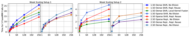
Figure 4: Weak scaling experiments with $r=256$. The horizontal axis gives the node count $p$ for each experiment. In setup 1, $p$ processors run FusedMM on $S$ of side-length $2^{16}p$ with 32 nonzeros per row. In setup 2, $p$ processors execute FusedMM on $S$ of side length $2^{16}p^{1/2}$ with $32p^{1/2}$ nonzeros per row.

To benchmark the weak scaling of our algorithms, we keep the FLOP count assigned to each node constant (assuming a load-balanced sparse matrix) while increasing both the processor count and the “problem size”. We investigated two methods of doubling the problem size, each giving different performance characteristics.

Setup 1: In these experiments, node counts double from experiment to experiment as we double the side-length of the sparse matrix, keeping the number of nonzeros in each row and the embedding dimension $r$ constant. We begin with sparse matrix dimensions $65536\times 65536$ on a single node with 32 nonzeros per row, and we use $r=256$ as the embedding dimension. We scale to 256 nodes that collectively process a $2^{24}\times 2^{24}$ matrix with 500 million nonzeros.

While FLOPs per processor remains constant from experiment to experiment, communication for our 1.5D algorithms scales as $O(n/\sqrt{p})$. Doubling both $n$ and $p$ results in an expected increase in communication time of $\sqrt{2}$, giving a projected $\sqrt{p}$-scaling in communication time with processor count. Similarly, our 2.5D algorithms have communication scaling of $O(n/\sqrt[3]{p^{2}})$, yielding a projected $\sqrt[3]{p}$ scaling in communication time with processor count. Notice also under this strategy that $\phi$ remains constant at $32/256=1/8$, while the percentage of nonzeros in $S$ decays exponentially. Figure 4 (left) gives the results of these experiments, for the best observed replication factor at each processor count. Even though each processor handles the same number of nonzeros across experiments, the communication time (detailed in figure 5) quickly dominates the computation time as we double the processor count. Among 1.5D algorithms, the sparse shifting, dense replicating algorithm exhibits the best overall performance. We attribute this to the low, constant value of $\phi=\textrm{nnz}(S)/nr$ across the experiments. At 256 nodes, replication reuse allows the replication reusing sparse shifting 1.5D algorithm to run 1.15 times faster than the 2.5D sparse replicating algorithm, while the variant without communication elision runs 2% slower than the 2.5D sparse replicating algorithm. For 1.5D dense shifting algorithms, both FusedMM elision strategies have roughly the same gain over the unoptimized back-to-back kernel sequence until the 256 node experiment. At 256 nodes, the 1.5D algorithm with local kernel fusion exhibits 1.38x speedup over its non-eliding counterpart, and replication reuse gives 1.16x speedup.

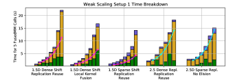
Figure 5: Weak scaling time breakdown, setup 1. Each section of bars indicates the time breakdown for successively doubling processor counts, from $p=2$ on the left of each subsection to $p=256$ on the right. We expect $p^{1/2}$-communication scaling for 1.5D algorithms and $p^{1/3}$ for 2.5D algorithms.

Setup 2: Beginning with the same conditions for a single node as setup 1, node counts quadruple from experiment to experiment, as we both double the side-length of the sparse matrix and double its nonzero count per row. The FLOPs per processor again remains constant. Under this setup, however, the percentage of nonzeros of $S$ remains constant while $\textrm{nnz}(S)/nr$ doubles from experiment to experiment. Setup 2 provides insight into the scaling of the 1.5D sparse shifting algorithm as the ratio $\phi$ successively doubles. Since the communication cost for 1.5D dense shifting algorithms does not depend on $\phi$ and scales as $O(n/\sqrt{p})$, its communication cost should remain constant across experiments, while the $O(n/\sqrt[3]{p^{2}})$ communication time scaling for 2.5D algorithms even implies a decrease in communication time. In practice, the decrease in node locality caused by scaling to high node counts renders a decrease in overall time unlikely.

Figure 4 (right half) shows the results, all of which take less than five seconds due to better communication scaling compared to setup 1. Inverting the results from the first weak scaling benchmark, the 1.5D sparse shifting algorithm performs progressively worse as node count increases compared to the best performer, the 1.5D dense shifting algorithm under local kernel fusion. At 256 nodes, the 1.5D local kernel fusion algorithm is 1.94 times as fast as the sparse shifting algorithm with replication reuse. For almost all cases, employing replication reuse or local kernel fusion results in nontrivial performance gains over an unoptimized sequence of SDDMM and SpMM.

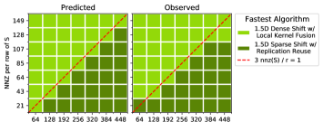
Figure 6: Predicted, Observed Optimal Algorithms for $p=32,m=2^{22}$. 2.5D algorithms were also benchmarked, but were neither predicted nor observed as best. The best observed replication factor in each configuration was used.

VI-C Effect of Embedding Width $r$

Compiled from 740 trials over different configurations, figure 6 shows the best algorithm out of the four that employ communication elision (along with the 2.5D sparse replicating algorithm) on a range of $r$-values and sparse matrix nonzero counts. As predicted, the 1.5D dense shifting algorithm performs better when $\phi=\textrm{nnz(S)}/nr$ is high, while the 1.5D sparse shifting algorithm performs better for low $\phi$. Both 1.5D algorithms outperform the 2.5D algorithms in theory as well as practice by margins comparable to those in figure 4. From figure 6, we note that the optimal algorithm choice is always a 1.5D sparse shifting or dense shifting algorithm depending on the value of $\phi$, a conclusion that carries some caveats. Specifically, the performance of the 2.5D algorithms is hurt at $p=32$ since the replication factor is constrained to be either 2 or 8. Our strong scaling experiments indicate that at high enough node counts, 2.5D algorithms approach (and sometimes outperform) the 1.5D algorithms.

For weak scaling setup 1, figure 7 gives the predicted and observed optimal replication factor as a function of the processor count for 1.5D dense shifting algorithms. As predicted, the optimal replication factor $c$ for the 1.5D algorithm with replication reuse is at least the optimal replication factor for the unfused algorithm. The latter, in turn, is at least the optimal replication factor of the local kernel fusion algorithm. The plot experimentally confirms that our fused algorithms save communication by changing the optimal replication factor in addition to decreasing the number of communication rounds.

Our predictions of optimal replication factor match the observed optimal values on most experiments. When they disagree, our theory tends to overestimate for two reasons: first, we did not test replication factors higher than 8 for our weak scaling experiments due to memory constraints, leading to the gap at the right end of the figure. Second, we used an ordering of MPI ranks that maximized locality within each layer of the processor grid. As a result, communication within the fiber axis (i.e. replication costs) are more expensive due to lack of node locality, a fact that we verified by comparing against an MPI rank order that optimized for locality along each fiber.

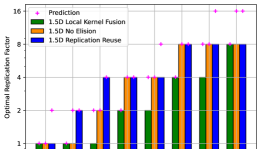
Figure 7: Predicted, Observed Optimal Replication Factors for Weak Scaling Experiments.

VI-D Strong Scaling on Real-World Matrices

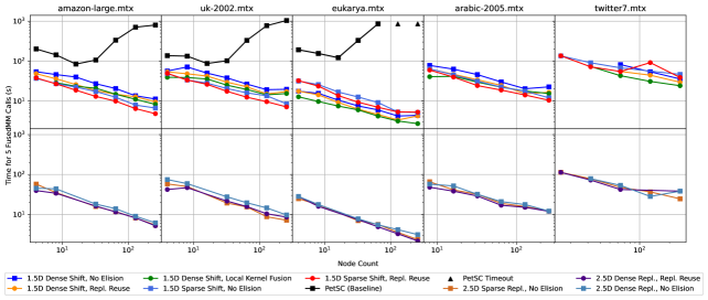
Figure 8: Strong scaling experiments, $r=128$. We benchmarked our algorithms on 5 FusedMM calls and the baseline implementation PETSc with 10 SpMM calls. Black triangles indicate that PETSc took longer than three hours to complete the trial. We benchmarked with a minimum of 4 nodes for the smaller workloads, 8 nodes for Arabic-2005, and 16 nodes for twitter7.

We conduct strong scaling experiments on up to 256 KNL nodes with $r=128$ on five real-world matrices given in table V containing up to $\approx 1.5$ billion nonzeros. amazon-large.mtx, uk-2002.mtx, arabic-2005.mtx, and twitter7.mtx were taken from the Suitesparse matrix collection [23], while eukarya.mtx contains protein sequence alignment information for eukaryotic genomes [24]. With $\approx 360$ million nonzeros but only $\approx 3$ million vertices, eukarya is the most dense at 111 nonzeros per row, compared with roughly 16 nonzeros per row for both uk-2002 and amazon-large. Twitter7 and Arabic-2005 fall between the two extremes at 28-35 nonzeros per row, but have significantly more total nonzeros compared to the other matrices. We expect that the 1.5D sparse shifting and 2.5D sparse replicating algorithms will exhibit better communication performance on the sparse Amazon matrix, while the 1.5D dense shifting and 2.5D dense replicating algorithms become optimal for eukarya and and twitter7. Because we choose $r=128$ conservatively to avoid allocating large amounts of RAM at small node counts, we enforce a minimum replication factor of 2 for the 1.5D sparse shifting algorithm at 256 nodes (since we cannot divide 128 into more than 256 parts for $c=1$).

Matrix	Rows	Columns	Nonzeros
amazon-large.mtx	14,249,639	14,249,639	230,788,269
uk-2002.mtx	18,484,117	18,484,117	298,113,762
eukarya.mtx	3,243,106	3,243,106	359,744,161
arabic-2005.mtx	22,744,080	22,744,080	639,999,458
twitter7.mtx	41,652,230	41,652,230	1,468,365,182

TABLE V: Matrices Used in Strong Scaling Experiments

Figure 8 gives the results of the strong scaling experiments; the performance of each algorithm is its best runtime over replication factors from 1 through 16. As we expect, the 1.5D sparse shifting algorithm with replication reuse performs best on the amazon-large and uk-2002 matrices, while it is the second worst on eukarya. With 256 nodes on uk-2002, the 1.5D sparse shifting algorithm with replication reuse performs 1.19x faster than the version without communication elision, and it performs 2.1x faster than the dense shifting fused algorithm with local kernel fusion. On eukarya with 256 nodes, the dense shifting algorithm with local kernel fusion performs 1.6x faster than the version without communication elision and 1.9x faster than the sparse shifting algorithm. Among 2.5D algorithms, the dense replicating algorithm with replication reuse and the sparse replicating algorithm have similar performance, and both outperform the 2.5D dense replicating algorithm with no communication elision. As predicted by our theory, the dense replicating algorithm has slightly better performance on eukarya.mtx at high node counts, even outperforming all of our 1.5D algorithms.

VI-E Applications

Here, we plug in our distributed memory algorithms to machine learning applications to benchmark their performance. We focus on two: collaborative filtering with alternating least squares, and graph neural networks with self-attention.

Collaborative Filtering with ALS: Collaborative filtering attempts to factor a matrix $C\in\mathbb{R}^{m\times n}$ as $C=AB^{T}$, for $A\in\mathbb{R}^{m\times r},B\in\mathbb{R}^{n\times r}$; however, we only have access to a set of sparse observations of $C$, denoted as the sparse matrix $\tilde{C}$ with nonzero indicators $S$. We iteratively minimize the loss, which is the Frobenius norm of $\tilde{C}-\textrm{SDDMM}(A,B,S)$. The SDDMM kernel in the loss also appears (along with SpMM) in the iterative update equations.

The ALS method alternately keeps $A$ or $B$ fixed and, for each row $x$ of the matrix to optimize for, solves a least squares problem of the form $Mx=b$. These least squares problems are distinct for each row due to the varying placement of nonzeros within each column of $S$. If we use Conjugate Gradients (CG) as the least squares solver, Zhao and Canny [1] exhibit the technique of batching computation of the query vectors $Mx$ for all rows at once using a FusedMM operation.

2.5D sparse replicating and 2.5D dense replicating algorithms suffer slight penalties for this application compared to 1.5D algorithms, as the output distributions of the dense matrices are shifted and transposed, respectively, compared to the input distributions. Since the output query vectors become (after some additional manipulation) inputs to the next CG iteration, 2.5D algorithms must pay to shift the input and output distributions at each step. We benchmark 20 CG iterations with our distributed algorithms embedded: 10 to optimize the matrix $A$, and 10 to optimize the matrix $B$.

Graph Attention Network (Forward Pass Workload): Consider a graph with adjacency matrix $S\in\{0,1\}^{n\times n}$. Conventional GNNs contain a series of layers, with an $r$-length vector of features associated with each node as the input to a layer. These node embeddings are held in an $n\times r$ matrix $A$, and the GNN layer applies a small linear transformation $W\in\mathbb{R}^{r\times r^{\prime}}$ to the embedding matrix before performing a convolution to sum the feature vectors at neighbors of any node $x$ as to become the new feature vector of $x$. Application of a nonlinear function $\sigma$, typically follows the convolution, giving the final layer output $A^{\prime}\in\mathbb{R}^{n\times r^{\prime}}$ as $A^{\prime}=\sigma(SAW)$.

The subsequent GNN layer takes $A^{\prime}$ as an input, with the final layer generating a node-level or graph-level prediction. Graph attention networks (GATs) modify this architecture by weighting edges with a self-attention score computed using the embeddings of the incident nodes. A single self-attention head [3] replaces $S$ with $S^{\prime}=\sigma_{\textrm{LeakyReLU}}(S*(A\cdot_{\mathit{GAT}}A^{T}))$. Here, $A\cdot_{\mathit{GAT}}A^{T}$ is an $n\times n$ matrix with entries given by $(A\cdot_{\mathit{GAT}}A^{T})_{ij}=a^{T}(A_{i:}||A_{j:})$, where $||$ denotes concatenation and $a^{T}$ is a trainable vector. The computation of $S^{\prime}$ involves a slight modification of Eq. 1 and has an identical communication pattern to SDDMM. A multi-head GAT concatenates the outputs of several attention heads with distinct trainable weight matrices $W$ and weight vectors $a$. We simulate the forward pass workload of this multi-head GAT architecture using random weight matrices to focus on the communication reduction and scaling of our distributed-memory algorithms.

Figure 9 shows the time breakdown of our applications, both inside the FusedMM kernels and in the rest of the application. The ALS application exhibits some variation in communication and computation time spent outside FusedMM. The variation is only partially due to additional processor to processor communication to compute distributed dot products, which is higher for the sparse replicating and shifting algorithms. More significantly, at the high replication factors (8 and 16) used in the experiment, the row-major local dense matrices are extremely tall-skinny for the 1.5D sparse shifting and 2.5D sparse replicating algorithms compared to the other variants. Careful analysis of the CG solver revealed that the dense batch dot product operation requires a long sequence of poorly performing dot product calls on short vectors. Since the sequence grows linearly with local matrix height, hundreds of thousands of these calls slow performance for the 1.5D sparse shifting and 2.5D sparse replicating algorithms. Calling an optimized batched BLAS library would fix this issue, which we leave as future work.

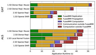
Figure 9: Alternating Least Squares and Graph Attention Network Forward Pass Performance on Amazon.mtx. We use 256 nodes and $r=128$. The 1.5D algorithm with local kernel fusion was not benchmarked for GATs, as it is incompatible with softmax regularization of learned edge weights.

VII Conclusions and Further Work

We gave a theoretical communication analysis of distributed memory sparsity agnostic approaches for SDDMM and FusedMM. Our theory predicted communication savings using two distinct approaches to combine the two kernels, and we observed those benefits in our strong and weak scaling experiments. In both theory and practice, 1.5D sparse shifting and 2.5D sparse replicating algorithms perform better when $S$ has far fewer nonzeros compared to either dense matrix. When $S$ has a higher nonzero count, dense shifting 1.5D and dense replicating 2.5D algorithms win out.

Further performance improvement may be possible by overlapping communication in the propagation phase of any of our algorithms with local computation. Such an implementation might require one-sided MPI or a similar protocol for remote direct memory access (RDMA) without CPU involvement.

Disclaimer

This report was prepared as an account of work sponsored by an agency of the United States Government. Neither the United States Government nor any agency thereof, nor any of their employees, makes any warranty, express or implied, or assumes any legal liability or responsibility for the accuracy, completeness, or usefulness of any information, apparatus, product, or process disclosed, or represents that its use would not infringe privately owned rights. Reference herein to any specific commercial product, process, or service by trade name, trademark, manufacturer, or otherwise does not necessarily constitute or imply its endorsement, recommendation, or favoring by the United States Government or any agency thereof. The views and opinions of authors expressed herein do not necessarily state or reflect those of the United States Government or any agency thereof.

References

- [1] J. Canny and H. Zhao, “Big Data Analytics with Small Footprint: Squaring the Cloud,” in KDD, 2013.
- [2] J. J. Tithi and F. Petrini, “An Efficient Shared-memory Parallel Sinkhorn-Knopp Algorithm to Compute the Word Mover’s Distance,” arXiv:2005.06727 [cs, stat], Mar. 2021, arXiv: 2005.06727.
- [3] P. Veličković, G. Cucurull, A. Casanova, A. Romero, P. Liò, and Y. Bengio, “Graph Attention Networks,” arXiv:1710.10903 [cs, stat], Feb. 2018, arXiv: 1710.10903.
- [4] M. Wang, D. Zheng, Z. Ye, Q. Gan, M. Li, X. Song, J. Zhou, C. Ma, L. Yu, Y. Gai, T. Xiao, T. He, G. Karypis, J. Li, and Z. Zhang, “Deep graph library: A graph-centric, highly-performant package for graph neural networks,” arXiv preprint arXiv:1909.01315, 2019.
- [5] C. Hong, A. Sukumaran-Rajam, I. Nisa, K. Singh, and P. Sadayappan, “Adaptive sparse tiling for sparse matrix multiplication,” in PPOPP. ACM, 2019, pp. 300–314.
- [6] I. Nisa, A. Sukumaran-Rajam, S. E. Kurt, C. Hong, and P. Sadayappan, “Sampled Dense Matrix Multiplication for High-Performance Machine Learning,” in HiPC, Dec. 2018, pp. 32–41.
- [7] P. Jiang, C. Hong, and G. Agrawal, “A novel data transformation and execution strategy for accelerating sparse matrix multiplication on GPUs,” in PPOPP, 2020, pp. 376–388.
- [8] P. Koanantakool, A. Azad, A. Buluç, D. Morozov, S.-Y. Oh, L. Oliker, and K. Yelick, “Communication-Avoiding Parallel Sparse-Dense Matrix-Matrix Multiplication,” in IPDPS, 2016, pp. 842–853.
- [9] O. Selvitopi, B. Brock, I. Nisa, A. Tripathy, K. Yelick, and A. Buluç, “Distributed-memory parallel algorithms for sparse times tall-skinny-dense matrix multiplication,” in ICS. ACM, 2021, pp. 431–442.
- [10] S. Acer, O. Selvitopi, and C. Aykanat, “Improving performance of sparse matrix dense matrix multiplication on large-scale parallel systems,” Parallel Computing, vol. 59, pp. 71–96, Nov. 2016.
- [11] M. K. Rahman, M. H. Sujon, and A. Azad, “FusedMM: A Unified SDDMM-SpMM Kernel for Graph Embedding and Graph Neural Networks,” in IPDPS, May 2021, pp. 256–266, iSSN: 1530-2075.
- [12] A. Tripathy, K. Yelick, and A. Buluç, “Reducing communication in graph neural network training,” in SC’20. IEEE, 2020, pp. 1–17.
- [13] L. E. Cannon, “A cellular computer to implement the kalman filter algorithm,” Ph.D. dissertation, USA, 1969, aAI7010025.
- [14] R. A. van de Geijn and J. Watts, “SUMMA: Scalable universal matrix multiplication algorithm,” USA, Tech. Rep., 1995.
- [15] E. Solomonik and J. Demmel, “Communication-Optimal Parallel 2.5D Matrix Multiplication and LU Factorization Algorithms,” in Euro-Par’11. Berlin, Heidelberg: Springer-Verlag, 2011, p. 90–109.
- [16] G. Kwasniewski, M. Kabić, M. Besta, J. VandeVondele, R. Solcà, and T. Hoefler, “Red-blue pebbling revisited: Near optimal parallel matrix-matrix multiplication,” in SC’19. ACM, 2019.
- [17] E. Chan, M. Heimlich, A. Purkayastha, and R. Van De Geijn, “Collective communication: theory, practice, and experience,” Concurrency and Comp.: Practice & Experience, vol. 19, no. 13, pp. 1749–1783, 2007.
- [18] “Cori - NERSC Documentation.” [Online]. Available: https://docs.nersc.gov/systems/cori/
- [19] A. Azad, O. Selvitopi, M. T. Hussain, J. Gilbert, and A. Buluç, “Combinatorial BLAS 2.0: Scaling combinatorial algorithms on distributed-memory systems,” IEEE TPDS, pp. 1–1, 2021.
- [20] G. Guennebaud, B. Jacob, and others, “Eigen v3,” 2010. [Online]. Available: http://eigen.tuxfamily.org
- [21] S. Balay, S. Abhyankar, M. F. Adams, S. Benson, J. Brown, P. Brune, K. Buschelman, E. Constantinescu, L. Dalcin, A. Dener, V. Eijkhout, W. D. Gropp, V. Hapla, T. Isaac, P. Jolivet, D. Karpeev, D. Kaushik, M. G. Knepley, F. Kong, S. Kruger, D. A. May, L. C. McInnes, R. T. Mills, L. Mitchell, T. Munson, J. E. Roman, K. Rupp, P. Sanan, J. Sarich, B. F. Smith, S. Zampini, H. Zhang, H. Zhang, and J. Zhang, “PETSc/TAO users manual,” Argonne National Laboratory, Tech. Rep. ANL-21/39 - Revision 3.16, 2021.
- [22] “Threads and PETSc — PETSc 3.16.2 documentation.” [Online]. Available: https://petsc.org/release/miscellaneous/threads/
- [23] T. A. Davis and Y. Hu, “The university of florida sparse matrix collection,” ACM Trans. Math. Softw., vol. 38, no. 1, dec 2011.
- [24] A. Azad, G. A. Pavlopoulos, C. A. Ouzounis, N. C. Kyrpides, and A. Buluç, “HipMCL: a high-performance parallel implementation of the Markov clustering algorithm for large-scale networks,” Nucleic Acids Research, vol. 46, no. 6, pp. e33–e33, 01 2018.